跳到论文正文
W Papers独立论文阅读器 arXiv:1907.04247 论文正文 计算阅读时间 · 0%
引用这篇论文根据当前论文元数据生成,正式投稿前建议核对。


License: arXiv.org perpetual non-exclusive license
arXiv:1907.04247v4 [math.NA] 13 Apr 2021

Dynamical low-rank integrator for the linear Boltzmann equation: error analysis in the diffusion limit

Zhiyan Ding Thanks: Department of Mathematics, University of Wisconsin-Madison, Madison, WI, 53706, USA (zding49@math.wisc.edu).    Lukas Einkemmer Thanks: Department of Mathematics, University of Innsbruck, Innsbruck, Austria (lukas.einkemmer@uibk.ac.at)    Qin Li Thanks: Department of Mathematics and Wisconsin Institute for Discovery, University of Wisconsin-Madison, Madison, WI, 53706, USA (qinli@math.wisc.edu).
Abstract

Dynamical low-rank algorithms are a class of numerical methods that compute low-rank approximations of dynamical systems. This is accomplished by projecting the dynamics onto a low-dimensional manifold and writing the solution directly in terms of the low-rank factors. The approach has been successfully applied to many types of differential equations. Recently, efficient dynamical low-rank algorithms have been proposed in [11, 14] to treat kinetic equations, including the Vlasov–Poisson and the Boltzmann equation. There it was demonstrated that the methods are able to capture the low-rank structure of the solution and significantly reduce numerical cost, while often maintaining high accuracy. However, no numerical analysis is currently available.

In this paper, we perform an error analysis for a dynamical low-rank algorithm applied to the multi-scale linear Boltzmann equation (a classical model in kinetic theory) to showcase the validity of the application of dynamical low-rank algorithms to kinetic theory. The equation, in its parabolic regime, is known to be rank one theoretically, and we will prove that the scheme can dynamically and automatically capture this low-rank structure. This work thus serves as the first mathematical error analysis for a dynamical low-rank approximation applied to a kinetic problem.

keywords
Dynamical low-rank approximation, multiscale analysis, linear Boltzmann equation, low-rank structure
††runningheads: Low rank integrator for the LBE / Zhiyan Ding, Lukas Einkemmer and Qin Li
AMS
65F55, 35L02, 65M06, 80A21

1 Introduction

Kinetic equations are a class of model equations used to describe the statistical behavior of a large number of particles that follow the same physical laws. They have been widely used in many aspects of physics and engineering. These equations, despite having different terms for various specific kinds of particles, share a similar structure: The dynamics is described in phase space and the solution is thus a distribution function u⁡(t,x,v)u(t,x,v) that counts the density of particles at a particular time tt, location xx, and velocity vv. One main challenge for the computation of kinetic equation comes from the fact that the equation is supported on phase space instead of physical space, and thus the dimensionality of the problem typically doubles.

During the past decade, numerous methods have been proposed to numerically solve kinetic equations and many of them succeed in reducing computational cost without sacrificing accuracy. The main body of work concentrates on developing fast solvers for the collision operators and overcoming the stability requirement of the time-discretization [24, 22], through either finding fast methods to treat the transport term [17, 47, 5, 12], or implementing the resulting discrete system efficiently [18, 13]. However, reducing the complexity due to the high dimensionality is largely left unaddressed. The difficulty here is rather clear. To compute PDEs, one needs to sample a certain amount of discrete points per dimension, and for kinetic equations that have high dimensionality, the degrees of freedom is large, driving up the numerical cost.

The viewpoint of degrees of freedom merely depending on the dimensionality of the problem was challenged in recent years, see [45] and references therein. In these works, the traditional approach is abandoned and one explores the structure of the intrinsic low-dimensional manifold where the PDE solution lives on. The method is designed to follow the flow of the dynamics and to identify the important features in the evolution. Since the equation is projected onto a solution manifold of lower dimensionality, only the core information is preserved and redundant information is neglected. The numerical cost thus depends mainly on the intrinsic dimensionality of the dynamics, rather than the total number of discrete points. The method was first utilized to deal with coupled ODE systems [39] and then was applied to a range of problems for which its accuracy has been demonstrated.

The success in dealing with ODE systems inspired the generalization to PDEs. More recently, a class of efficient numerical schemes were proposed for computing kinetic equations, including the Vlasov–Poisson system [28, 14], the Vlasov-Maxwell system  [16] and the classical Boltzmann equation [11] in both collisionless and strong-collisional regimes. In these experiments, it was observed that both the sophisticated Landau damping phenomenon for the VP system [48, 44], and the incompressible Navier-Stokes limit for the Boltzmann equation are captured rather accurately at very low cost. Different equations may require slightly modified dynamical low-rank algorithms to suit the specific structures of the equation, but the general approach is quite similar. The main features in the evolution are preserved by following the flow of the equation projected onto the low dimensional solution manifold.

However, despite the strong intuition and the many promising numerical experiments, rigorous mathematical analysis is largely absent, especially in the PDE setting. There are two major difficulties, one from the theoretical level, and one is numerical. First, we often do not have results to show that the true solution is indeed approximately of low-rank. This point is more subtle than one might think. In fact, a Fourier expansion is also a low-rank approximation. But, a Fourier expansion uses a fixed set of basis functions, and the prediction of the rank is higher than the intrinsic rank of the solution. In addition, showing the low rank structure by performing a Fourier decomposition relies on assuming smoothness of the solution, which for kinetic equations is certainly problematic. It should be noted, however, that for elliptic equations some results can be obtained [6].

The second difficulty is numerical: How to show the method can capture the low-rank structure of the solution? For the ODE case an analysis has been performed in [26] and related works, but this analysis only applies to the non-stiff case and is thus not applicable to PDEs. The only mathematical analysis of a dynamical low-rank scheme in the PDE setting we are aware of is found in [46]. This paper considers a special situation where the stiffness originates only from the linear differential operator whose corresponding flow is exactly computable within the low-rank formulation. This separation suggests a splitting procedure that decouples the stiff and non-stiff dynamics, which permits a convergence analysis of the resulting method. This is not the situation for kinetic equations, and thus the analysis does not apply.

In this paper, we will consider a multi-scale linear Boltzmann equation. The equation is equipped with a parameter called the Knudsen number, and when it is small, the equation has a strong collision operator, and is in the diffusive scaling. It is a well known result that when this happens, the solution reduces to a rank 11 function, namely the solution can be written as a multiplication of two functions, one for xx and one for vv respectively. The first challenge mentioned above therefore turns out to be trivial in this case. In this particular paper, we aim at solving the second challenge, which is to prove the dynamical low-rank algorithm can indeed capture this low rank structure. More specifically, we will show, through utilizing the Hilbert expansion, that in the small Knudsen number limit, the method automatically captures the rank 11 behavior of the solution. These results imply that compared to the traditional approaches that require discretization of the full phase space, the essential degrees of freedom only scale as the number of grid points in physical space.

We should mention that the results shown here only address the low-rank dynamics of the linear Boltzmann equation. It is a showcase for the validity of the algorithm on kinetic equations, and serves as a stepping stone for future studies on more complicated kinetic equations. We also stress that although the linear Boltzmann equation itself is linear, the studied dynamical low-rank algorithm is nonlinear and involved, making the proof highly non-trivial. We report the analytical result showing the performance of different time-integrators, discussing both advantages and disadvantages in the asymptotic regimes.

1.1 Multi-scale linear Boltzmann equation

We first give a quick overview of the equation. In d>1d>1 dimension, let (t,x,v)∈ℝ+×Ωx×𝒮d−1(t,x,v)\in\mathbb{R}^{+}\times\Omega_{x}\times\mathcal{S}^{d-1}, the equation writes:

∂tu(t,x,v)=ℒu=−vϵ⋅∇xu(t,x,v)+σ⁡(x)ϵ2(ρ(x)−u(t,x,v)),\partial_{t}u(t,x,v)=\mathcal{L}u=-\frac{v}{\epsilon}\cdot\nabla_{x}u(t,x,v)+\frac{\sigma(x)}{\epsilon^{2}}\left(\rho(x)-u(t,x,v)\right)\,, (1)

where σ⁡(x)\sigma(x) is the scattering cross-section, Ωx⊂ℝd\Omega_{x}\subset\mathbb{R}^{d}, ϵ\epsilon is called the Knudsen number, which represents the ratio between the mean free path and the typical domain length, and vv is the angular variable. Since v∈𝒮d−1v\in\mathcal{S}^{d-1}, the unit sphere in dd dimensional space, all vv have the same amplitude. The density ρ\rho is defined as follows

ρ⁡(x)=⟨u⁡(t,x,v)⟩v=1|𝒮d−1|​∫𝒮d−1u⁡(t,x,v)​𝑑v,\rho(x)=\langle u(t,x,v)\rangle_{v}=\frac{1}{|\mathcal{S}^{d-1}|}\int_{\mathcal{S}^{d-1}}u(t,x,v)\,\mathrm{d}{v}\,, (2)

where |𝒮d−1||\mathcal{S}^{d-1}| is the volume of 𝒮d−1\mathcal{S}^{d-1} and ⟨⋅⟩v\langle\cdot\rangle_{v} denotes the average with respect to v∈𝒮d−1v\in\mathcal{S}^{d-1}. For the sake of convenience we shorten the notation

d​μv=1|𝒮d−1|​d​v,\,\mathrm{d}\mu_{v}=\frac{1}{|\mathcal{S}^{d-1}|}\,\mathrm{d}v\,,

where d​μv\,\mathrm{d}\mu_{v} is the normalized measure in v∈𝒮d−1v\in\mathcal{S}^{d-1}. The equation is written in diffusion scaling, meaning the transport term v⋅∇xuv\cdot\nabla_{x}u and the collision term ρ−u\rho-u are enlarged by 1ϵ\frac{1}{\epsilon} and 1ϵ2\frac{1}{\epsilon^{2}}, respectively.

It is a well-known result that when ϵ→0\epsilon\to 0, the solution uu of (1) will asymptotically approach ρ\rho and thus becomes vv independent. Furthermore, ρ\rho solves the heat equation, with CdC_{d} being a constant that depends on dd only:

∂tρ=∇x⋅(1Cd​σ​(x)​∇xρ),(t,x)∈ℝ+×Ωx.\partial_{t}\rho=\nabla_{x}\cdot\left(\frac{1}{C_{d}\sigma(x)}\nabla_{x}\rho\right)\,,\quad(t\,,x)\in\mathbb{R}^{+}\times\Omega_{x}\,. (3)

For this reason, this is termed the parabolic regime, and the limit is called the diffusion limit. For this paper, this limit is particularly interesting because it essentially shows that u⁡(t,x,v)∼ρ⁡(t,x)u(t,x,v)\sim\rho(t,x) is approximately of rank 11.

There are two difficulties in computing this equation. First, when the Knudsen number ϵ\epsilon is small, both the transport term and the collision operator are stiff. A traditional numerical method would require small time stepsize that resolves the stiffness. Second, equation (1) is posed in an 2​d−12d-1 dimensional phase space. Suppose the equation has NxN_{x} grid points per spatial direction and NvN_{v} grid points per velocity direction, then Nxd​Nvd−1N_{x}^{d}N_{v}^{d-1} floating point numbers are needed. The large increase in the degrees of freedom is usually referred to as the curse of dimensionality in the literature.

There are indeed techniques developed to enlarge the stability region to overcome the stiffness problem as mentioned in the first challenge. In the kinetic framework, it is usually referred to as asymptotic preserving [21, 7, 30, 3, 9, 34, 8, 29]. Also see reviews [20, 23, 10]. However, the investigation into the second problem is mostly open. The belief that numerical cost mostly depends on the number of grid points and thus the degrees of freedom has been so firm, and essentially has not been challenged in the literature till the proposal of the dynamical low-rank approximation.

1.2 Dynamical low rank approximation

Dynamical low rank approximation is a systematic approach to tackle the curse of dimensionality for time-dependent problems. Believing that the number of grid points usually over-represent the necessary numerical information, the main aim of the approximation is to explore the rank structure of the solution manifold. Instead of seeking the solution on a fixed set of grid points, the method evolves the low rank representation, and characterizes the flow of the solution on a low dimensional manifold.

There are many ways to decompose the solution into its low rank presentation. For kinetic equations in particular, it is rather straightforward to separate the physical space and the velocity space:

u⁡(t,x,v)=∑i,j=1rSi,j​Xi​(t,x)​Vj​(t,v),u(t,x,v)=\sum^{r}_{i,j=1}S_{i,j}X_{i}(t,x)V_{j}(t,v)\,, (4)

so that the low rank factors XiX_{i} and VjV_{j} depend only on either xx or vv respectively. In the formula, rr is the rank, and is typically significantly smaller than min​(Nx,Nv)\text{min}(N_{x},N_{v}). For this presentation, the number of degrees of freedom is O⁡(r⁡(Nxd+Nvd−1))O(r\left(N^{d}_{x}+N^{d-1}_{v}\right)).

Historically, dynamical low-rank approximations have been considered extensively in high dimensional problems arising in quantum mechanics. Finding a low rank approximation there makes the computation tractable, see [43, 42] and [36, 37, 4] for a mathematical treatment. The application of the method in a general setting is studied in [26, 27, 40, 1], where both the matrix and the general tensor formats are investigated. In the initial development, one significant disadvantage was observed: the methods are not robust with respect to over-approximation. Several strategies were proposed to address the issue, including both regularization, and the projector splitting integrator. The latter is viewed as a major improvement [39] in enhancing the robustness with respect to small singular values [25]. This approach was later extended to various tensor formats [37, 38, 19, 41], and is the approach to be utilized in this paper.

The application of dynamical low-rank approximation for kinetic equations is relatively recent. Numerical experiments have been performed on the Vlasov–Poisson [14, 15], the Vlasov–Maxwell [16], and the Boltzmann equation [11], and the numerical evidence is very promising. However, theoretical justification have been lacking.

In particular, from a mathematical point of view we need to answer two questions

  1. 1.

    When do the solutions have low-rank structures?

  2. 2.

    Can dynamical low-rank approximation capture this structure?

The first question, in the kinetic framework, would be addressed by utilizing the fluid limit justification, as shown in (1) and (3). Since one can show that as ϵ→0\epsilon\to 0 we get u⁡(t,x,v)=ρ⁡(t,x)u(t,x,v)=\rho(t,x), the velocity direction completely degenerates, and the rank of the representation in equation (4) is simply 11. It is then reasonable to expect that for small ϵ\epsilon the solution is only slightly different from its rank-11 approximation.

To address the second question relies on proper algorithm-design. As mentioned above, we will use the projector-splitting approach. This leads to a set of three evolution equations for SS, XX, and VV, respectively, and all three will be advanced in every single time step in a proper order. It turns out that the specific time integrator for each equation plays a crucial role. More specifically, we will show that the implicit Euler method, due to the lack of symmetry, requires fine time discretization for capturing the rank structure, while the Crank–Nicolson–Implicit–Euler (CNIE) method will converge with very relaxed constraints on the time step size but does require well-prepared initial data. Note that in the CNIE method we use the Crank–Nicolson scheme for XX and SS and the implicit Euler scheme for VV. We propose to use the implicit Euler method for the initial step and a very small time stepsize, to reveal the structure of the PDE solution, and then switch to CNIE to preserve this structure.

The rest of the paper is organized as follows. In Section 2 we present the application of the dynamical low-rank projector splitting integrator to the linear Boltzmann equation. Both the semi-discrete splitting scheme and the fully-discrete methods are presented, in Section 2.1 and 2.2 respectively. In Section 3 we state and prove the main results. In Section 3.1 we study the numerical cost saving and an intuitive explanation of the error analysis is presented in Section 3.2. Section 3.3 and 3.4 are dedicated to the error analysis with the implicit Euler and CNIE time integrator respectively, and we summarize the analysis with a final proposal of an algorithm in Section 3.5. Some parts of the proof in Section 3 are rather tedious, and we leave them to Appendix. Numerical evidences are presented in Section 4.

2 Numerical scheme

We present the application of the dynamical low-rank approximation method to the linear Boltzmann equation in this section. We follow the framework and notations in [14]. Throughout the paper we use the standard L2L^{2} vector space in both the spatial and the velocity domain. That is, we have

⟨f,g⟩x=∫f⁡(x)​g​(x)​𝑑x,⟨f,g⟩v=∫f⁡(v)​g​(v)​d​μv.\langle f,g\rangle_{x}=\int f(x)g(x)\,\mathrm{d}{x}\,,\quad\langle f,g\rangle_{v}=\int f(v)g(v)\,\mathrm{d}\mu_{v}\,.

We call a function f⁡(x,v)f(x,v) a rank-rr function if it can be expanded by a set of rr orthonormal basis functions in xx and vv. All these functions are collected to the set ℳ\mathcal{M}:

Definition 1 (Rank-rr function in L2​(d​x​d​v)L_{2}(\,\mathrm{d}x\,\mathrm{d}v)).

The collection of all rank-rr functions is denoted by

ℳ={f⁡(x,v)∈L2​(Ωx×𝒮d−1):f⁡(x,v)​ is rank-​r},\mathcal{M}=\left\{f(x,v)\in L^{2}(\Omega_{x}\times\mathcal{S}^{d-1}):f(x,v)\text{ is rank-}r\right\},

where f⁡(x,v)f(x,v) is rank-rr, meaning: f⁡(x,v)=∑i,j=1rSi,j​Xi​(x)​Vj​(v)f(x,v)=\sum^{r}_{i,j=1}S_{i,j}X_{i}(x)V_{j}(v) where XiX_{i} and ViV_{i} being orthonormal in physical and velocity space respectively:

⟨Xi,Xj⟩x=∫ΩxXi​Xj​𝑑x=δi​j,⟨Vi,Vj⟩v=∫𝒮d−1Vi​Vj​d​μv=δi​j.\left\langle X_{i}\,,X_{j}\right\rangle_{x}=\int_{\Omega_{x}}X_{i}X_{j}\,\mathrm{d}x=\delta_{ij},\quad\left\langle V_{i}\,,V_{j}\right\rangle_{v}=\int_{\mathcal{S}^{d-1}}V_{i}V_{j}\,\mathrm{d}\mu_{v}=\delta_{ij}\,.

We note that in this definition, only the rank, rr, is fixed. The basis functions XiX_{i} and VjV_{j} can be arbitrary, as long as the orthogonality condition is satisfied. We further emphasize that ℳ\mathcal{M} is not a function space; it is easily seen that the summation of two rank-rr functions may not be rank-rr.

It is unlikely that the solution is of rank-rr, i.e. in ℳ\mathcal{M}, for all time. However, numerically one can argue that the solution is approximately of low rank. Thus for the numerical solution we seek a rank-rr approximation in ℳ\mathcal{M} at every time step. The algorithm is consequently looking for a trajectory on the manifold ℳ\mathcal{M} that resembles the evolution guided by the equation. In some sense, we need to project the equation in L2​(Ω×𝒮d−1)L^{2}(\Omega\times\mathcal{S}^{d-1}) to the manifold and find the equation that governs the dynamics of this trajectory in ℳ\mathcal{M}.

We denote by u⁡(t,x,v)u(t,x,v) the analytic solution and by ur​(t,x,v)u_{r}(t,x,v) the numerical rank-rr approximation, then with the argument above, the governing equation for uru_{r} is

∂tur=𝒫ur​(ℒ​ur)=𝒫ur​(σ⁡(x)ϵ2​(ρ−ur)−vϵ⋅∇xur),\partial_{t}u_{r}=\mathcal{P}_{u_{r}}(\mathcal{L}u_{r})=\mathcal{P}_{u_{r}}\left(\frac{\sigma(x)}{\epsilon^{2}}\left(\rho-u_{r}\right)-\frac{v}{\epsilon}\cdot\nabla_{x}u_{r}\right)\,, (5)

where 𝒫u​f\mathcal{P}_{u}f stands for the projection of ff onto the tangential plane of ℳ\mathcal{M} at uu. Denoting 𝒯ur​ℳ\mathcal{T}_{u_{r}}\mathcal{M} the tangential plane of ℳ\mathcal{M} at uru_{r}, this projection operator ensures

u˙r∈𝒯ur​ℳ,\dot{u}_{r}\in\mathcal{T}_{u_{r}}\mathcal{M}\,,

guaranteeing that uru_{r} lies in the manifold ℳ\mathcal{M} for all time.

We now look for explicitly expression of the tangential plane and the projection operator. For a nonlinear manifold ℳ\mathcal{M}, such expressions necessarily depend on the point where the tangent is looked for. Denote

f=∑i​jSi​j​Xi​Vj∈Span​{Xi}i=1r⊗Span​{Vj}j=1r,f=\sum_{ij}S_{ij}X_{i}V_{j}\in\text{Span}\{X_{i}\}_{i=1}^{r}\otimes\text{Span}\{V_{j}\}_{j=1}^{r}\,,

then the tangential plane is given by

𝒯f​ℳ={g∈L2(dxdv):g=∑ri,j=1Xi(x)S˙i,jVj(v)+X˙i(x)Si,jVj(v)+Xi(x)Si,jV˙j(v)withS˙∈ℝr×r,X˙i∈L2(Ωx),V˙j∈L2(𝒮d−1),and⟨Xi,X˙j⟩x=⟨Vi,V˙j⟩v=0}.\begin{aligned} &\mathcal{T}_{f}{\mathcal{M}}\\ &=\left\{g\in L^{2}(\,\mathrm{d}x\,\mathrm{d}v)\,:g=\sum^{r}_{i,j=1}X_{i}(x)\dot{S}_{i,j}V_{j}(v)+\dot{X}_{i}(x)S_{i,j}V_{j}(v)+X_{i}(x)S_{i,j}\dot{V}_{j}(v)\right.\\ &\left.\text{with}\ \dot{S}\in\mathbb{R}^{r\times r},\dot{X}_{i}\in L^{2}(\Omega_{x}),\dot{V}_{j}\in L^{2}(\mathcal{S}^{d-1})\,,\text{and}\left\langle X_{i},\dot{X}_{j}\right\rangle_{x}=\left\langle V_{i},\dot{V}_{j}\right\rangle_{v}=0\right\}\end{aligned}\,.

This set collects all functions whose infinitesimal, when added to ff, still yields a rank-rr function. In this definition, we notice that we are allowed to choose arbitrarily an r×rr\times r matrix S˙\dot{S}, a function list X˙i\dot{X}_{i} and a function list V˙i\dot{V}_{i}, as long as the gauge conditions, ⟨Xi,X˙j⟩x=⟨Vi,V˙j⟩v=0\left\langle X_{i},\dot{X}_{j}\right\rangle_{x}=\left\langle V_{i},\dot{V}_{j}\right\rangle_{v}=0, are satisfied. We note that the gauge conditions are imposed to guarantee the uniqueness of the low-rank factors. Interested readers are referred to [39] for details.

With this definition, one has:

𝒫f​g=𝒫X​g+𝒫V​g−𝒫V​𝒫X​g,∀g∈L2​(Ωx×𝒮d−1),\mathcal{P}_{f}g=\mathcal{P}_{{X}}g+\mathcal{P}_{{V}}g-\mathcal{P}_{{V}}\mathcal{P}_{{X}}g,\quad\forall g\in L^{2}(\Omega_{x}\times\mathcal{S}^{d-1})\,, (6)

where the spatial and velocity projection are

𝒫X​g=∑ir⟨Xi,g⟩x​Xi,𝒫V​g=∑ir⟨Vi,g⟩v​Vi,𝒫V​𝒫X​g=∑i,jrXi​⟨Xi​Vj,g⟩x,v​Vj.\displaystyle\mathcal{P}_{{X}}g=\sum^{r}_{i}\langle X_{i},g\rangle_{x}X_{i}\,,\quad\mathcal{P}_{{V}}g=\sum^{r}_{i}\langle V_{i},g\rangle_{v}V_{i}\,,\quad\mathcal{P}_{{V}}\mathcal{P}_{X}g=\sum^{r}_{i,j}X_{i}\langle X_{i}V_{j},g\rangle_{x,v}V_{j}\,.

Inserting (6) into (5) gives us the governing equation for uru_{r}:

∂tur=𝒫ur​(ℒ​ur)=(𝒫Xur+𝒫Vur−𝒫Vur​𝒫Xur)​(ℒ​ur).\partial_{t}u_{r}=\mathcal{P}_{u_{r}}(\mathcal{L}u_{r})=\left(\mathcal{P}_{X_{u_{r}}}+\mathcal{P}_{V_{u_{r}}}-\mathcal{P}_{V_{u_{r}}}\mathcal{P}_{X_{u_{r}}}\right)(\mathcal{L}u_{r})\,. (7)

The numerical method will then be developed upon this formulation. We discuss the semi-discrete (in time) and the fully-discrete schemes (both implicit Euler and CNIE) in details in the following subsections.

2.1 Semi-discrete low rank splitting method

In this section, we develop a projector-splitting method to solve equation (7). In order to be concise, we simply denote the low rank solution uru_{r} by uu and we decompose the solution using its low-rank representation:

u⁡(t,x,v)=∑i,j=1rXi​(t,x)​Si,j​(t)​Vj​(t,v)=X⁡(t,x)​S​(t)​V⊤​(t,v)=X⁡(t,x)​L​(t,v)=K⁡(t,x)​V⊤​(t,v),\begin{aligned} u(t,x,v)&=\sum^{r}_{i,j=1}X_{i}(t,x)S_{i,j}(t)V_{j}(t,v)\\ &=\mathrm{X}(t,x)\mathrm{S}(t)\mathrm{V}^{\top}(t,v)=\mathrm{X}(t,x)\mathrm{L}(t,v)=\mathrm{K}(t,x)\mathrm{V}^{\top}(t,v)\end{aligned}\,, (8)

where X\mathrm{X} and V\mathrm{V} collects the basis functions

{X⁡(t,x)=[X1​(t,x),X2​(t,x),…,Xr​(t,x)],V⁡(t,v)=[V1​(t,v),V2​(t,v),…,Vr​(t,v)].\displaystyle\begin{cases}\mathrm{X}(t,x)=\left[X_{1}(t,x),X_{2}(t,x),\dots,X_{r}(t,x)\right]\,,\\ \mathrm{V}(t,v)=\left[V_{1}(t,v),V_{2}(t,v),\dots,V_{r}(t,v)\right]\,.\end{cases}

We will also be using quantities K\mathrm{K} and L\mathrm{L}:

L⁡(t,v)=S⁡(t)​V⊤​(t,v)=[L1​(t,v),L2​(t,v),…,Lr​(t,v)]⊤,\displaystyle\mathrm{L}(t,v)=\mathrm{S}(t)\mathrm{V}^{\top}(t,v)=\left[L_{1}(t,v),L_{2}(t,v),\dots,L_{r}(t,v)\right]^{\top}, (9)
K⁡(t,x)=X⁡(t,x)​S​(t)=[K1​(t,x),K2​(t,x),…,Kr​(t,x)].\displaystyle\mathrm{K}(t,x)=\mathrm{X}(t,x)\mathrm{S}(t)=\left[K_{1}(t,x),K_{2}(t,x),\dots,K_{r}(t,x)\right]\,. (10)

Computing (7) at discrete times tnt_{n} amounts to finding the governing equations that provide the updates of

Xn,Vn,andSn,\mathrm{X}^{n}\,,\quad\mathrm{V}^{n}\,,\quad\text{and}\quad\mathrm{S}^{n},

respectively, for all tnt_{n} with n≥1n\geq 1.

To specify the initial data, we project the initial condition onto ℳ\mathcal{M} using the singular value decomposition (SVD), namely:

u⁡(t=0,x,v)≈∑i,j=1rXi​(t=0,x)​Si,j​(t=0)​Vj​(t=0,v)=X0​(x)​S0​(V0​(v))T.u(t=0,x,v)\approx\sum^{r}_{i,j=1}X_{i}(t=0,x)S_{i,j}(t=0)V_{j}(t=0,v)=\mathrm{X}^{0}(x)\mathrm{S}^{0}(\mathrm{V}^{0}(v))^{\mathrm{T}}\,. (11)

For updating X,V,S\mathrm{X,V,S}, the Lie-Trotter splitting is used. From time step tnt_{n} to tn+1=tn+Δ​tt_{n+1}=t_{n}+\Delta t, we split the three operators on the right hand side of (7) into three sub-steps:

∂tu\displaystyle\partial_{t}u =𝒫Xu​(σ⁡(x)ϵ2​(ρ−u)−vϵ⋅∇xu),\displaystyle=\mathcal{P}_{\mathrm{X}_{u}}\left(\frac{\sigma(x)}{\epsilon^{2}}\left(\rho-u\right)-\frac{v}{\epsilon}\cdot\nabla_{x}u\right), (12)
∂tu\displaystyle\partial_{t}u =−𝒫Vu​𝒫Xu​(σ⁡(x)ϵ2​(ρ−u)−vϵ⋅∇xu),\displaystyle=-\mathcal{P}_{\mathrm{V}_{u}}\mathcal{P}_{\mathrm{X}_{u}}\left(\frac{\sigma(x)}{\epsilon^{2}}\left(\rho-u\right)-\frac{v}{\epsilon}\cdot\nabla_{x}u\right), (13)
∂tu\displaystyle\partial_{t}u =𝒫Vu​(σ⁡(x)ϵ2​(ρ−u)−vϵ⋅∇xu).\displaystyle=\mathcal{P}_{\mathrm{V}_{u}}\left(\frac{\sigma(x)}{\epsilon^{2}}\left(\rho-u\right)-\frac{v}{\epsilon}\cdot\nabla_{x}u\right). (14)

This splitting (12)-(14) takes place for each time step. That is, given the numerical solution at time tnt_{n} we update the solution to tn+1t_{n+1} by solving the three equations one after another. All equations are advanced for a full time step Δ​t\Delta t. Different from directly solving (7), each sub-step only changes one part of the decomposition. In particular, the first splitting step (12) preserves X\mathrm{X}, the last (14) preserves V\mathrm{V}, and the middle step (13) merely updates S\mathrm{S}. This allows us to update the three components separately. Below we detail the evolution of each sub-step:

  1. 1.

    Updating (12):

    Starting with un​(x,v)=Xn​(x)​Sn​(Vn​(v))⊤u^{n}(x,v)=\mathrm{X}^{n}(x)\mathrm{S}^{n}\left(\mathrm{V}^{n}(v)\right)^{\top}, we run (12) for a full time step Δ​t\Delta t, and we denote the result by un+1/3​(x,v)u^{n+1/3}(x,v). The step preserves X\mathrm{X} and thus:

    Xn+1/3​(x)=Xn​(x).\mathrm{X}^{n+1/3}(x)=\mathrm{X}^{n}(x)\,.

    To update Sn+1/3\mathrm{S}^{n+1/3} and Vn+1/3\mathrm{V}^{n+1/3}, we plug the low rank formulation (8) into (12) and obtain, for 1≤i≤r1\leq i\leq r:

    ∂tLi=−1ϵ∑rj=1⟨Xni,v⋅∇Xnj⟩xLj+1ϵ2∑rj=1⟨Xni,σXnj⟩x(⟨Lj⟩v−Lj),\displaystyle\partial_{t}L_{i}=-\frac{1}{\epsilon}\sum^{r}_{j=1}\left\langle X^{n}_{i},v\cdot\nabla X^{n}_{j}\right\rangle_{x}L_{j}+\frac{1}{\epsilon^{2}}\sum^{r}_{j=1}\left\langle X^{n}_{i},\sigma X^{n}_{j}\right\rangle_{x}\left(\langle L_{j}\rangle_{v}-L_{j}\right)\,,

    By using equation (9) we can simplify it to:

    ∂tL(t,v)=−1ϵ∑k=1dvkA∂knL(t,v)+1ϵ2Aσn(⟨L(t,⋅)⟩v−L(t,v)),\partial_{t}\mathrm{L}(t,v)=-\frac{1}{\epsilon}\sum^{d}_{k=1}v_{k}\mathrm{A}^{n}_{\partial_{k}}\mathrm{L}(t,v)+\frac{1}{\epsilon^{2}}\mathrm{A}^{n}_{\sigma}\left(\left\langle\mathrm{L}(t,\cdot)\right\rangle_{v}-\mathrm{L}(t,v)\right), (15)

    where v=[v1,⋯,vd]v=[v_{1}\,,\cdots\,,v_{d}], and A∂kn\mathrm{A}^{n}_{\partial_{k}} and Aσn\mathrm{A}^{n}_{\sigma}, both ∈ℝr×r\in\mathbb{R}^{r\times r}, are matrix versions of the differential operator and the scattering operator respectively:

    [A∂kn]i,j=⟨Xin,∂kXjn⟩x,(1≤k≤d),\displaystyle\left[\mathrm{A}^{n}_{\partial_{k}}\right]_{i,j}=\left\langle X^{n}_{i}\,,\partial_{k}X^{n}_{j}\right\rangle_{x},\;(1\leq k\leq d)\,, (16)
    [Aσn]i,j=⟨Xin,σ​Xjn⟩x.\displaystyle\left[\mathrm{A}^{n}_{\sigma}\right]_{i,j}=\left\langle X^{n}_{i},\sigma X^{n}_{j}\right\rangle_{x}\,.

    We denote the solution of (15) by Ln+1/3​(v)\mathrm{L}^{n+1/3}(v), and Sn+1/3\mathrm{S}^{n+1/3} and Vn+1/3​(v)\mathrm{V}^{n+1/3}(v) are obtained through the Gram-Schmidt process (QR factorization) which ensures the orthogonality of Vn+1/3​(v)\mathrm{V}^{n+1/3}(v):

    Ln+1/3​(v)=Sn+1/3​(Vn+1/3​(v))⊤.\mathrm{L}^{n+1/3}(v)=\mathrm{S}^{n+1/3}\left(\mathrm{V}^{n+1/3}(v)\right)^{\top}\,.

    Finally:

    un+1/3=(XSV⊤)n+1/3.u^{n+1/3}=(\mathrm{X}\mathrm{S}\mathrm{V}^{\top})^{n+1/3}\,.
  2. 2.

    Updating (13): In this step, equation (13) is evolved for Δ​t\Delta t with initial condition un+1/3u^{n+1/3}. Since the step only changes S\mathrm{S}, we immediately obtain

    Xn+2/3=Xn+1/3,andVn+2/3=Vn+1/3.\mathrm{X}^{n+2/3}=\mathrm{X}^{n+1/3}\,,\quad\text{and}\quad\mathrm{V}^{n+2/3}=\mathrm{V}^{n+1/3}\,.

    Plugging the low rank representation (8) into (13), we obtain, in matrix form:

    ∂tS⁡(t)=1ϵ​∑k=1dA∂kn​S​(t)​Ξvkn+2/3−1ϵ2​Aσn​S​(t)​Γn+2/3,\partial_{t}\mathrm{S}(t)=\frac{1}{\epsilon}\sum^{d}_{k=1}\mathrm{A}^{n}_{\partial_{k}}\mathrm{S}(t)\mathrm{\Xi}^{n+2/3}_{v_{k}}-\frac{1}{\epsilon^{2}}\mathrm{A}^{n}_{\sigma}\mathrm{S}(t)\mathrm{\Gamma}^{n+2/3}\,, (17)

    where Ξvk\mathrm{\Xi}_{v_{k}} and Γ\mathrm{\Gamma}, both ∈ℝr×r\in\mathbb{R}^{r\times r}, are the matrix versions of the multiplication operator associated to vkv_{k} (1≤k≤d1\leq k\leq d) and the density term, respectively:

    [Ξvk]i,j=⟨Vi​(⋅),(⋅)k​Vj​(⋅)⟩v,and[Γ]i,j=⟨Vi​(⋅)⟩v​⟨Vj​(⋅)⟩v−δi,j.\displaystyle\left[\mathrm{\Xi}_{v_{k}}\right]_{i,j}=\left\langle V_{i}(\cdot),(\cdot)_{k}V_{j}(\cdot)\right\rangle_{v}\,,\quad\text{and}\quad\left[\mathrm{\Gamma}\right]_{i,j}=\langle V_{i}(\cdot)\rangle_{v}\langle V_{j}(\cdot)\rangle_{v}-\delta_{i,j}\,. (18)

    We denote the computed update of (17) by Sn+2/3\mathrm{S}^{n+2/3} and

    un+2/3=(XSV⊤)n+2/3.u^{n+2/3}=(\mathrm{X}\mathrm{S}\mathrm{V}^{\top})^{n+2/3}\,.
  3. 3.

    Updating (14):

    In this step, (14) is evolved for a full time step Δ​t\Delta t with initial value un+2/3u^{n+2/3}. This step preserves V\mathrm{V}. Thus,

    Vn+1​(v)=Vn+2/3​(v)⇒Ξn+1=Ξn+2/3,andΓn+1=Γn+2/3.\mathrm{V}^{n+1}(v)=\mathrm{V}^{n+2/3}(v)\quad\Rightarrow\quad\mathrm{\Xi}^{n+1}=\mathrm{\Xi}^{n+2/3}\,,\quad\text{and}\quad\mathrm{\Gamma}^{n+1}=\mathrm{\Gamma}^{n+2/3}\,.

    To update Xn+1\mathrm{X}^{n+1} and Sn+1\mathrm{S}^{n+1}, the low rank formulation (8) is plugging into (12). In the matrix form we have:

    ∂tK⁡(t,x)+1ϵ​∑k=1d∂kK⁡(t,x)​Ξvkn+1=1ϵ2​K​(t,x)​Γn+1.\partial_{t}\mathrm{K}(t,x)+\frac{1}{\epsilon}\sum^{d}_{k=1}\partial_{k}\mathrm{K}(t,x)\mathrm{\Xi}^{n+1}_{v_{k}}=\frac{1}{\epsilon^{2}}\mathrm{K}(t,x)\mathrm{\Gamma}^{n+1}\,. (19)

    Solving this equation we obtain Kn+1​(v)\mathrm{K}^{n+1}(v), and the orthogonality of Xn+1\mathrm{X}^{n+1} is ensured through the Gram-Schmidt process:

    Kn+1​(x)=Xn+1​Sn+1.\mathrm{K}^{n+1}(x)=\mathrm{X}^{n+1}\mathrm{S}^{n+1}\,.

With these three steps completed, one finally arrives at the numerical solution at time tn+1t_{n+1}

un+1=(XSV⊤)n+1.u^{n+1}=\left(\mathrm{X}\mathrm{S}\mathrm{V}^{\top}\right)^{n+1}\,.
Remark 1.

We describe the method without incorporating special boundary conditions. The problem is assumed to be a Cauchy problem with infinite boundary. In the numerical examples and the theorems that we prove below, we used periodic boundary condition to eliminate the possible complication induced by the boundary. If Dirichlet-type boundary condition is provided, the incoming data may drive the solution away from the low rank approximation, and a boundary layer that sees drastic changes in both xx and vv space is needed to damp the fluctuation. Recent analysis in this direction can be found in [49, 31, 32, 33] and the references therein.

2.2 Fully-discrete low rank splitting method

We discretize the aforementioned splitting method in time and phase space. We denote

𝒳={x1,x2​…,xNx},𝒱={v1,v2​…,vNv}\mathcal{X}=\left\{x_{1},x_{2}\dots,x_{N_{x}}\right\}\,,\quad\mathcal{V}=\left\{v_{1},v_{2}\dots,v_{N_{v}}\right\} (20)

the sets of discrete points in Ωx\Omega_{x} and 𝒮d−1\mathcal{S}^{d-1}. The discrete solution can then be represented as follows

ℝNx×Nv∋un=𝖷n​𝖲n​(𝖵n)⊤,\mathbb{R}^{N_{x}\times N_{v}}\ni u^{n}=\mathsf{X}^{n}\mathsf{S}^{n}(\mathsf{V}^{n})^{\top}\,,

where 𝖲n=Sn\mathsf{S}^{n}=\mathrm{S}^{n} and we abuse the notation by calling

𝖷n=[X1n​X2n​…​Xrn]∈ℝNx×r,and𝖵n=[V1n​V2n​…​Vrn]∈ℝNv×r\mathsf{X}^{n}=\left[X^{n}_{1}\ X^{n}_{2}\ \dots\ X^{n}_{r}\right]\in\mathbb{R}^{N_{x}\times r}\,,\quad\text{and}\quad\mathsf{V}^{n}=\left[V^{n}_{1}\ V^{n}_{2}\ \dots\ V^{n}_{r}\right]\in\mathbb{R}^{N_{v}\times r} (21)

with XinX^{n}_{i} and VinV^{n}_{i} denoting the ii-th mode evaluated at the grid points.

We now perform an implicit time integration of the three equations (15), (17), and (19) to overcome the stability issue introduced by the stiffness.

  • –

    For updating (15), 𝖷n+1/3=𝖷n\mathsf{X}^{n+1/3}=\mathsf{X}^{n}. Applying the implicit Euler scheme gives

    {𝖫n+1/3−𝖫nΔ​t+1ϵ​∑k=1d𝖠∂kn​𝖫n+1/3​Πvk=𝖠σnϵ2​𝖫n+1/3​𝖢,QR decomposition: 𝖫n+1/3=𝖲n+1/3(𝖵n+1)⊤.\left\{\begin{aligned} &\frac{\mathsf{L}^{n+1/3}-\mathsf{L}^{n}}{\Delta t}+\frac{1}{\epsilon}\sum^{d}_{k=1}\mathsf{A}^{n}_{\partial_{k}}\mathsf{L}^{n+1/3}\mathsf{\Pi}_{v_{k}}=\frac{\mathsf{A}^{n}_{\sigma}}{\epsilon^{2}}\mathsf{L}^{n+1/3}\mathsf{C}\,,\\ &\text{QR decomposition: }\mathsf{L}^{n+1/3}=\mathsf{S}^{n+1/3}(\mathsf{V}^{n+1})^{\top}\,.\end{aligned}\right. (22)

    or applying the Crank–Nicolson method (first step of CNIE) gives

    {𝖫n+1/3−𝖫nΔ​t+1ϵ​∑k=1d𝖠∂kn​(𝖫n+1/3+𝖫n2)​Πvk=𝖠σnϵ2​𝖫n+1/3+𝖫n2​𝖢,QR decomposition: 𝖫n+1/3=𝖲n+1/3(𝖵n+1/3)⊤.\left\{\begin{aligned} &\frac{\mathsf{L}^{n+1/3}-\mathsf{L}^{n}}{\Delta t}+\frac{1}{\epsilon}\sum^{d}_{k=1}\mathsf{A}^{n}_{\partial_{k}}\left(\frac{\mathsf{L}^{n+1/3}+\mathsf{L}^{n}}{2}\right)\mathsf{\Pi}_{v_{k}}=\frac{\mathsf{A}^{n}_{\sigma}}{\epsilon^{2}}\frac{\mathsf{L}^{n+1/3}+\mathsf{L}^{n}}{2}\mathsf{C}\,,\\ &\text{QR decomposition: }\mathsf{L}^{n+1/3}=\mathsf{S}^{n+1/3}(\mathsf{V}^{n+1/3})^{\top}\,.\end{aligned}\right. (23)

    In the equation we have used

    𝖠n∂k=(𝖷n)⊤𝖣k𝖷n,𝖠nσ=𝖷⊤Σ𝖷,\displaystyle\mathsf{A}^{n}_{\partial_{k}}=(\mathsf{X}^{n})^{\top}\mathsf{D}_{k}\mathsf{X}^{n}\,,\quad\mathsf{A}^{n}_{\sigma}=\mathsf{X}^{\top}\mathsf{\Sigma}\mathsf{X}\,, (24)
    Πvk=diag(𝒱k),𝖢=1Nvee⊤−𝖨Nv,\displaystyle\mathsf{\Pi}_{v_{k}}=\text{diag}(\mathcal{V}_{k})\,,\quad\mathsf{C}=\frac{1}{N_{v}}ee^{\top}-\mathsf{I}_{N_{v}}\,,

    with e=(1,1,…,1)⊤e=\left(1,1,\dots,1\right)^{\top}. Σ=diag​(σ​(𝒳))\mathsf{\Sigma}=\text{diag}(\sigma(\mathcal{X})) is an Nx×NxN_{x}\times N_{x} matrix with evaluations of σ\sigma at the grid points in 𝒳\mathcal{X} assigned as diagonal entries and 𝖣k\mathsf{D}_{k} is the discrete approximation of ∂xk\partial_{x_{k}}. The specific form of 𝖣k\mathsf{D}_{k} depends on the spatial discretization. We have used the simple rectangle rule for the integration in μv\mu_{v}. This determines the form of 𝖢\mathsf{C}. Other numerical integral rules could also be applied and the specific form of 𝖢\mathsf{C} will change accordingly. Obviously 𝖠∂kn\mathsf{A}^{n}_{\partial_{k}} and 𝖠σn\mathsf{A}^{n}_{\sigma} are the discrete versions of (16).

  • –

    For updating (17), we note that 𝖷\mathsf{X} and 𝖵\mathsf{V} are preserved:

    𝖷n+2/3=𝖷n+1/3,and𝖵n+2/3=𝖵n+1/3.\mathsf{X}^{n+2/3}=\mathsf{X}^{n+1/3}\,,\quad\text{and}\quad\mathsf{V}^{n+2/3}=\mathsf{V}^{n+1/3}\,.

    The direct application of the implicit Euler scheme gives

    𝖲n+2/3−𝖲n+1/3Δ​t−1ϵ​∑k=1d𝖠∂kn​𝖲n+2/3​Ξvkn+2/3=−𝖠σnϵ2​𝖲n+2/3​Γn+2/3.\frac{\mathsf{S}^{n+2/3}-\mathsf{S}^{n+1/3}}{\Delta t}-\frac{1}{\epsilon}\sum^{d}_{k=1}\mathsf{A}^{n}_{\partial_{k}}\mathsf{S}^{n+2/3}\mathsf{\Xi}^{n+2/3}_{v_{k}}=-\frac{\mathsf{A}^{n}_{\sigma}}{\epsilon^{2}}\mathsf{S}^{n+2/3}\mathsf{\Gamma}^{n+2/3}\,. (25)

    Similarly, if Crank–Nicolson (second step of CNIE) is used , the scheme reads

    𝖲n+2/3−𝖲n+1/3Δ​t−1ϵ​∑k=1d𝖠∂kn​𝖲n+2/3+𝖲n+1/32​Ξvkn+2/3\displaystyle\frac{\mathsf{S}^{n+2/3}-\mathsf{S}^{n+1/3}}{\Delta t}-\frac{1}{\epsilon}\sum^{d}_{k=1}\mathsf{A}^{n}_{\partial_{k}}\frac{\mathsf{S}^{n+2/3}+\mathsf{S}^{n+1/3}}{2}\mathsf{\Xi}^{n+2/3}_{v_{k}} (26)
    =\displaystyle= −𝖠σnϵ2​𝖲n+2/3+𝖲n+1/32​Γn+2/3.\displaystyle-\frac{\mathsf{A}^{n}_{\sigma}}{\epsilon^{2}}\frac{\mathsf{S}^{n+2/3}+\mathsf{S}^{n+1/3}}{2}\mathsf{\Gamma}^{n+2/3}\,.

    Here Ξvkn+2/3\mathsf{\Xi}^{n+2/3}_{v_{k}} and Γn+2/3\mathsf{\Gamma}^{n+2/3}, both r×rr\times r, are discrete versions of (18):

    Ξvkn+2/3=(𝖵n+2/3)⊤​Πvk​𝖵n+2/3,Γn+2/3=(𝖵n+2/3)⊤​𝖢𝖵n+2/3.\mathsf{\Xi}^{n+2/3}_{v_{k}}=(\mathsf{V}^{n+2/3})^{\top}\mathsf{\Pi}_{v_{k}}\mathsf{V}^{n+2/3}\,,\quad\mathsf{\Gamma}^{n+2/3}=(\mathsf{V}^{n+2/3})^{\top}\mathsf{C}\mathsf{V}^{n+2/3}\,. (27)
  • –

    Finally for updating (19), we note

    𝖵n+1=𝖵n+2/3,Γn+1=Γn+2/3,Ξn+1=Ξn+2/3.\mathsf{V}^{n+1}=\mathsf{V}^{n+2/3}\,,\quad\mathsf{\Gamma}^{n+1}=\mathsf{\Gamma}^{n+2/3}\,,\quad\mathsf{\Xi}^{n+1}=\mathsf{\Xi}^{n+2/3}\,.

    Defining:

    𝖪n+2/3=𝖷n+2/3​𝖲n+2/3,\mathsf{K}^{n+2/3}=\mathsf{X}^{n+2/3}\mathsf{S}^{n+2/3}\,, (28)

    we apply the implicit Euler method for

    {𝖪n+1−𝖪n+2/3Δ​t+1ϵ​∑k=1d𝖣k​𝖪n+1​Ξvkn+1=Σϵ2​𝖪n+1​Γn+1,QR decomposition:𝖷n+1𝖲n+1=𝖪n+1.\left\{\begin{aligned} &\frac{\mathsf{K}^{n+1}-\mathsf{K}^{n+2/3}}{\Delta t}+\frac{1}{\epsilon}\sum^{d}_{k=1}\mathsf{D}_{k}\mathsf{K}^{n+1}\mathsf{\Xi}^{n+1}_{v_{k}}=\frac{\mathsf{\Sigma}}{\epsilon^{2}}\mathsf{K}^{n+1}\mathsf{\Gamma}^{n+1}\,,\\ &\text{QR decomposition:}\ \mathsf{X}^{n+1}\mathsf{S}^{n+1}=\mathsf{K}^{n+1}\,.\end{aligned}\right. (29)

    The Crank–Nicolson method will not be used in the last step and thus we do not specify it.

We finalize the update for

un+1=𝖷n+1​𝖲n+1​(𝖵n+1)⊤.u^{n+1}=\mathsf{X}^{n+1}\mathsf{S}^{n+1}(\mathsf{V}^{n+1})^{\top}\,.

We stress that the choice of 𝖣k\mathsf{D}_{k} is not straightforward. Indeed, in the ϵ→0\epsilon\to 0 limit, a term 𝖣k​Σ−1​𝖣k\mathsf{D}_{k}\Sigma^{-1}\mathsf{D}_{k} will appear as the discretization of the Laplacian term. To guarantee the self-adjointness on the discrete level, 𝖣k\mathsf{D}_{k} needs to be specifically chosen. For more details see Remark 8.

We summarize the one-time step integrators in Algorithm 1 and 2.

Algorithm 1 One-timestep implicit Euler integrator
Input:
1. time step Δ​t\Delta t;
2. Input data: 𝖷n\mathsf{X}^{n}, 𝖲n\mathsf{S}^{n} and 𝖵n\mathsf{V}^{n}.
Run:
  • •

    Construct 𝖠∂kn,𝖠σn\mathsf{A}^{n}_{\partial_{k}},\mathsf{A}^{n}_{\sigma} by (24); Compute 𝖫n=𝖲n​(𝖵n)⊤\mathsf{L}^{n}=\mathsf{S}^{n}(\mathsf{V}^{n})^{\top};

  • –

    Update 𝖫n+1/3\mathsf{L}^{n+1/3} by solving (22) with Δ​t\Delta t;

  • •

    Perform QR decomposition to obtain 𝖲n+1/3,𝖵n+1\mathsf{S}^{n+1/3},\mathsf{V}^{n+1} from (22); Construct Ξvkn+1\mathsf{\Xi}^{n+1}_{v_{k}} and Γn+1\mathsf{\Gamma}^{n+1} by (27);

  • –

    Update 𝖲n+2/3\mathsf{S}^{n+2/3} with Δ​t\Delta t by solving (25);

  • •

    Construct 𝖪n+2/3=𝖷n​𝖲n+2/3\mathsf{K}^{n+2/3}=\mathsf{X}^{n}\mathsf{S}^{n+2/3} by (28);

  • –

    Update 𝖪n+1\mathsf{K}^{n+1} with Δ​t\Delta t by solving (29);

  • •

    Perform QR decomposition to obtain 𝖷n+1,𝖲n+1\mathsf{X}^{n+1},\mathsf{S}^{n+1} from (29);

Output: Numerical solution 𝖷n+1,𝖲n+1,𝖵n+1\mathsf{X}^{n+1},\mathsf{S}^{n+1},\mathsf{V}^{n+1};
Algorithm 2 One-timestep Crank–Nicolson–Implicit–Euler (CNIE) integrator
Input:
1. time step Δ​t\Delta t;
2. Input data: 𝖷n\mathsf{X}^{n}, 𝖲n\mathsf{S}^{n} and 𝖵n\mathsf{V}^{n}.
Run:
  • •

    Construct 𝖠∂kn,𝖠σn\mathsf{A}^{n}_{\partial_{k}},\mathsf{A}^{n}_{\sigma} by (24); Compute 𝖫n=𝖲n​(𝖵n)⊤\mathsf{L}^{n}=\mathsf{S}^{n}(\mathsf{V}^{n})^{\top};

  • –

    Update 𝖫n+1/3\mathsf{L}^{n+1/3} by solving (23) with Δ​t\Delta t;

  • •

    Perform QR decomposition to obtain 𝖲n+1/3,𝖵n+1\mathsf{S}^{n+1/3},\mathsf{V}^{n+1} from (23); Construct Ξvkn+1\mathsf{\Xi}^{n+1}_{v_{k}} and Γn+1\mathsf{\Gamma}^{n+1} by (27);

  • –

    Update 𝖲n+2/3\mathsf{S}^{n+2/3} with Δ​t\Delta t by solving (26);

  • •

    Construct 𝖪n+2/3=𝖷n​𝖲n+2/3\mathsf{K}^{n+2/3}=\mathsf{X}^{n}\mathsf{S}^{n+2/3} by (28);

  • –

    Update 𝖪n+1\mathsf{K}^{n+1} with Δ​t\Delta t by solving (29);

  • •

    Perform QR decomposition to obtain 𝖷n+1,𝖲n+1\mathsf{X}^{n+1},\mathsf{S}^{n+1} from (29);

Output: Numerical solution 𝖷n+1,𝖲n+1,𝖵n+1\mathsf{X}^{n+1},\mathsf{S}^{n+1},\mathsf{V}^{n+1};

3 Properties of the numerical scheme

We investigate the properties of the numerical method in this section. In particular we will discuss the computational complexity and prove that the method captures the rank-11 structure in the parabolic regime.

3.1 Computational complexity

To analyze the computational complexity is rather straightforward. Denote rr the rank, NxN_{x} and NvN_{v} the cardinality of 𝒳\mathcal{X} and 𝒱\mathcal{V} respectively. The matrices in the updating formula, 𝖷n\mathsf{X}^{n}, 𝖲n\mathsf{S}^{n}, 𝖵n\mathsf{V}^{n} are computed by solving (22), (25), (29). The cost is summarized in Table 1:

Operations floating point operations(flops)
Calculation of 𝖠∂kn\mathsf{A}^{n}_{\partial_{k}},𝖠σn\mathsf{A}^{n}_{\sigma} (24) O⁡(r2​Nx)O(r^{2}N_{x})
Preparation of 𝖫n\mathsf{L}^{n} O⁡(r2​Nv)O(r^{2}N_{v})
Total cost of preparation O⁡(r2​(Nv+Nx))O(r^{2}(N_{v}+N_{x}))
Calculation of Πvk⊗𝖠∂kn\mathsf{\Pi}_{v_{k}}\otimes\mathsf{A}^{n}_{\partial_{k}}, 𝖢⊗𝖠σn\mathsf{C}\otimes\mathsf{A}^{n}_{\sigma} O⁡(r2​Nv)O(r^{2}N_{v})
Solving 𝖫n+1\mathsf{L}^{n+1} (22) O⁡(r3​Nv3)O(r^{3}N^{3}_{v})
Total cost of updating 𝖫\mathsf{L} O⁡(r3​Nv3)O(r^{3}N^{3}_{v})
QR decomposition to obtain 𝖲n+1/3\mathsf{S}^{n+1/3}, 𝖵n+1/3\mathsf{V}^{n+1/3} O⁡(r2​Nv)O(r^{2}N_{v})
Calculation of Ξvkn+2/3\mathsf{\Xi}^{n+2/3}_{v_{k}} and Γn+2/3\mathsf{\Gamma}^{n+2/3} (27) O⁡(r2​Nv)O(r^{2}N_{v})
Calculation of Ξvkn+2/3⊗𝖠∂kn\mathsf{\Xi}^{n+2/3}_{v_{k}}\otimes\mathsf{A}^{n}_{\partial_{k}}, Γn+2/3⊗𝖠σn\mathsf{\Gamma}^{n+2/3}\otimes\mathsf{A}^{n}_{\sigma} O⁡(r3)O(r^{3})
Solving 𝖲n+2/3\mathsf{S}^{n+2/3} (26) O⁡(r6)O(r^{6})
Total cost of updating 𝖲\mathsf{S} O⁡(r6+r2​Nv)O(r^{6}+r^{2}N_{v})
Preparation of 𝖪n+2/3\mathsf{K}^{n+2/3} (28) O⁡(r2​Nx)O(r^{2}N_{x})
Calculation of Ξvkn+2/3⊗𝖣k\mathsf{\Xi}^{n+2/3}_{v_{k}}\otimes\mathsf{D}_{k}, Γn+2/3⊗Σ\mathsf{\Gamma}^{n+2/3}\otimes\mathsf{\Sigma} O⁡(r2​Nx)O(r^{2}N_{x})
Solving 𝖪n+1\mathsf{K}^{n+1} (29) O⁡(r3​Nx3)O(r^{3}N^{3}_{x})
Total cost of updating 𝖪\mathsf{K} O⁡(r3​Nx3)O(r^{3}N^{3}_{x})
QR decomposition to obtain 𝖷n+1\mathsf{X}^{n+1}, 𝖲n+1\mathsf{S}^{n+1} O⁡(r2​Nx)O(r^{2}N_{x})
Total cost of one time step O⁡(r3​(r3+Nv3+Nx3))O(r^{3}(r^{3}+N^{3}_{v}+N^{3}_{x}))
Table 1: Floating point operation required for the dynamical low-rank algorithm. We note that in the computation of 𝖫n+1\mathsf{L}^{n+1}, 𝖲n+2/3\mathsf{S}^{n+2/3} and 𝖪n+1\mathsf{K}^{n+1} we used the classical LU decomposition. These steps can be sped up in implementation with iterative algorithms such as Krylov iteration. We leave out the discussion for this part of computational saving.

Because r=O⁡(1)≪min​{Nx,Nv}r=O(1)\ll\text{min}\{N_{x}\,,N_{v}\}, in conclusion, we need O⁡(Nx3+Nv3)O(N^{3}_{x}+N^{3}_{v}) flops per time step, instead of the O⁡(Nx3​Nv3)O(N^{3}_{x}N^{3}_{v}) as required by the traditional solvers.

3.2 Intuition of the error analysis

Before describing and proving our results in detail, in this section we first give a relatively vague justification on why the method works. As described in the introduction, there are two points we need to make:

  • •

    Why the true solution has an approximate low rank structure? This question is a rather fundamental, and is independent of the method chosen: the rank structure of the solution purely depends on the governing PDE we are studying here.

  • •

    Why the method keeps track of the low rank structure? This question concerns the behavior of the specific method (dynamical low-rank approximation) we choose to use here.

To answer the first question, we merely cite the following result.

Theorem 2 (Theorem 2 of [2]).

Denote uϵu^{\epsilon} the solution to the linear Boltzmann equation, for (t,x,v)∈ℝ+×Ωx×𝒮d−1(t,x,v)\in\mathbb{R}^{+}\times\Omega_{x}\times\mathcal{S}^{d-1}:

∂tuϵ=ℒ​uϵ=σϵ2​ℒ0​uϵ+1ϵ​ℒ1​uϵ,\partial_{t}u^{\epsilon}=\mathcal{L}u^{\epsilon}=\frac{\sigma}{\epsilon^{2}}\mathcal{L}_{0}u^{\epsilon}+\frac{1}{\epsilon}\mathcal{L}_{1}u^{\epsilon}\,, (30)

where ℒ0​u=ρ−u\mathcal{L}_{0}u=\rho-u and ℒ1u=−v⋅∇xu\mathcal{L}_{1}u=-v\cdot\nabla_{x}u. Then in the zero limit of ϵ\epsilon, the solution converges to the solution of the diffusion equation ∂tρ=∇x⋅(1d​σ​∇xρ)\partial_{t}\rho=\nabla_{x}\cdot\left(\frac{1}{d\sigma}\nabla_{x}\rho\right) in the sense that

‖uϵ​(t,x,v)−ρ⁡(t,x)‖L2​(d​x​d​μ)≤C​ϵ,\|u^{\epsilon}(t,x,v)-\rho(t,x)\|_{L_{2}(\,\mathrm{d}x\,\mathrm{d}\mu)}\leq C\epsilon\,,

where CC has no dependence on ϵ\epsilon.

We note that periodic boundary conditions are imposed in the original theorem to avoid complications that may come from boundary layers. Essentially this theorem states that in the zero limit of ϵ\epsilon, uϵ​(t,x,v)u^{\epsilon}(t,x,v) loses its velocity dependence, and the dynamics will purely be reflected in the physical space. In some sense:

uϵ​(t,x,v)=ρ⁡(x)+𝒪⁡(ϵ),u^{\epsilon}(t,x,v)=\rho(x)+\mathcal{O}(\epsilon)\,,

can be seen as the rank-11 approximation with the threshold set at any value bigger than ϵ\epsilon.

The proof for the theorem uses the Hilbert expansion. Formally, one writes uϵ=u0+ϵ​u1+ϵ2​u2+⋯u^{\epsilon}=u_{0}+\epsilon u_{1}+\epsilon^{2}u_{2}+\cdots and performs an asymptotic analysis. Showing Theorem 2 rigorously then amounts to bounding u2u_{2} uniformly in ϵ\epsilon (this exposition is rather lengthy and we omit it here).

To answer the second question amounts to proving that the dynamical low-rank approximation captures the rank structure of the solution. To do so, we recall

∂tur=𝒫ur​ℒ​ur=𝒫ur​[1ϵ2​ℒ0​ur+1ϵ​ℒ1​ur].\partial_{t}u_{r}=\mathcal{P}_{u_{r}}\mathcal{L}u_{r}=\mathcal{P}_{u_{r}}\left[\frac{1}{\epsilon^{2}}\mathcal{L}_{0}u_{r}+\frac{1}{\epsilon}\mathcal{L}_{1}u_{r}\right]. (31)

Notice that the equation differs from its continuous counterpart (30) by the projection 𝒫ur\mathcal{P}_{u_{r}} on the right hand side. The key to the analysis is two-folded:

  • •

    Showing that the projection operator 𝒫ur\mathcal{P}_{u_{r}} does not disturb the rank-11 structure of the solution;

  • •

    Showing that upon the projection, the leading order of the numerical solution follows the correct dynamics.

To show the former, we mimic the analysis on the PDE level, and perform the asymptotic analysis for (31) by setting ur=ur,0+ϵ​ur,1+⋯u_{r}=u_{r,0}+\epsilon u_{r,1}+\cdots. Then in the leading order:

𝒪⁡(1ϵ2):𝒫ur​ℒ0​ur,0=0.\mathcal{O}\left(\frac{1}{\epsilon^{2}}\right):\quad\mathcal{P}_{u_{r}}\mathcal{L}_{0}u_{r,0}=0\,.

Note that if we suppose ur∈Span​{Xi}⊗Span​{Vj}u_{r}\in\text{Span}\{X_{i}\}\otimes\text{Span}\{V_{j}\}, then with the definition of ℒ0\mathcal{L}_{0},

ℒ0​ur=ρ−ur=⟨ur⟩v−ur∈Span​{Xi}⊗Span​{Vj}⇒𝒫ur​ℒ0​ur,0=ℒ0​ur,0=0.\mathcal{L}_{0}u_{r}=\rho-u_{r}=\langle u_{r}\rangle_{v}-u_{r}\in\text{Span}\{X_{i}\}\otimes\text{Span}\{V_{j}\}\quad\Rightarrow\quad\mathcal{P}_{u_{r}}\mathcal{L}_{0}u_{r,0}=\mathcal{L}_{0}u_{r,0}=0\,.

This suggests that 𝒫ur\mathcal{P}_{u_{r}}, at least in the leading order, does not induce new rank structure, and thus one has ur,0∈Null​ℒ0u_{r,0}\in\mathrm{Null}\mathcal{L}_{0}, making uru_{r} approximately rank-11. To show that ur,0u_{r,0} follows the right equilibrium flow requires more delicate derivations in the higher order expansions, and we leave the details to Section 3.

3.3 Asymptotic analysis of the implicit Euler method

To unify the notation, throughout this section, we denote by unu^{n} a matrix of size Nx×NvN_{x}\times N_{v} with ui​jnu^{n}_{ij} being the numerical solution at tn,xi,vjt_{n},x_{i},v_{j}. Denote e=[1,⋯,1]⊤e=[1,\cdots,1]^{\top} a column vector of length NvN_{v}, en=e/Nve_{\mathrm{n}}=e/\sqrt{N_{v}} the normalized version, then ρn=un​e\rho^{n}=u^{n}e is a vector of length NxN_{x} representing the discrete version of ρ\rho at time tnt_{n} for spatial grid points 𝒳\mathcal{X}. The hope is to show that density ρn\rho^{n} solves equation (3) in the limit ϵ→0\epsilon\to 0.

Our first result concerns the behavior of the implicit Euler method in the asymptotic regime. The corresponding result, stated in Theorem 3, is shown under the following technical assumption.

Assumption 1.

For all nn, there exists an orthogonal matrix 𝖰n∈ℝr×r\mathsf{Q}^{n}\in\mathbb{R}^{r\times r} such that

𝖵n,∗=𝖵n​𝖰n\displaystyle\mathsf{V}^{n,*}=\mathsf{V}^{n}\mathsf{Q}^{n} (32)
=\displaystyle= (en,𝒱1,n+ϵ​a1,𝒱2,n+ϵ​a2,…,𝒱d,n+ϵ​ad,Vd+2∗,…,Vr∗)+O⁡(ϵ2),\displaystyle\left(e_{\mathrm{n}}\,,\mathcal{V}_{1,\mathrm{n}}+\epsilon a_{1}\,,\mathcal{V}_{2,\mathrm{n}}+\epsilon a_{2}\,,\dots,\mathcal{V}_{d,\mathrm{n}}+\epsilon a_{d}\,,V^{*}_{d+2},\dots,V^{*}_{r}\right)+O(\epsilon^{2})\,,

where the components satisfy (for all 1≤k≤d1\leq k\leq d and i≥d+2i\geq d+2)

en⊤​ak=O⁡(ϵ),(𝒱k,n)⊤​Vin+1,∗=O⁡(ϵ),en⊤​Vin+1,∗=O⁡(ϵ2).\displaystyle e^{\top}_{\mathrm{n}}a_{k}=O(\epsilon),\ \left(\mathcal{V}_{k,\mathrm{n}}\right)^{\top}V^{n+1,*}_{i}=O(\epsilon),\ e^{\top}_{\mathrm{n}}V^{n+1,*}_{i}=O(\epsilon^{2})\,. (33)

Here 𝒱i=[(v1)i,(v2)i,⋯(vNv)i]⊤\mathcal{V}_{i}=[(v_{1})_{i}\,,(v_{2})_{i}\,,\cdots(v_{N_{v}})_{i}]^{\top} collects the ii-th dimension component of all coordinates in 𝒱\mathcal{V}. Since v∈ℝdv\in\mathbb{R}^{d}, the subindex of 𝒱i\mathcal{V}_{i} changes from 11 to dd. We further denote the normalization by 𝒱i,n=dNv​𝒱i\mathcal{V}_{i,\mathrm{n}}=\frac{\sqrt{d}}{\sqrt{N_{v}}}\mathcal{V}_{i}.

Remark 2 (Intuition of Assumption 1).

To understand this assumption we link it to the proof for the diffusion limit in the continuous setting. For proving Theorem 2, it is expected that

uϵ=u0+ϵ​u1+ϵ2​u2,u^{\epsilon}=u_{0}+\epsilon u_{1}+\epsilon^{2}u_{2}\,,

where u0u_{0} has no vv dependence and u1∼v⋅∇xu0u_{1}\sim v\cdot\nabla_{x}u_{0}. This means the leading order of the equation should be homogeneous in vv and the next order linearly reflects vv in every dimension. This is presented in the definition of 𝖵n,∗\mathsf{V}^{n,\ast} where ene_{\mathrm{n}} and 𝒱i\mathcal{V}_{i} present homogeneity and linearity in the leading and the next order respectively.

There are direct consequences of this assumption. Define αn=(𝖵n)⊤​en\alpha^{n}=(\mathsf{V}^{n})^{\top}e_{\mathrm{n}} and αn,∗=(𝖵n,∗)⊤​en\alpha^{n,*}=(\mathsf{V}^{n,*})^{\top}e_{\mathrm{n}}, then

αn=𝖰​αn,∗,αn,∗=(𝖵n,∗)⊤​en=(1+O⁡(ϵ4),O⁡(ϵ2),…,O⁡(ϵ2))⊤.\alpha^{n}=\mathsf{Q}\alpha^{n,\ast},\quad\alpha^{n,*}=(\mathsf{V}^{n,*})^{\top}e_{\mathrm{n}}=\left(1+O(\epsilon^{4}),O(\epsilon^{2}),\dots,O(\epsilon^{2})\right)^{\top}\,. (34)

Similarly, let

Ξvkn,∗=(𝖵n,∗)⊤​Πvk​𝖵n=𝖰⊤​Ξvkn​𝖰,andΓn,∗=(𝖵n,∗)⊤​𝖢𝖵n=𝖰⊤​Γn​𝖰,\mathsf{\Xi}^{n,\ast}_{v_{k}}=(\mathsf{V}^{n,*})^{\top}\Pi_{v_{k}}\mathsf{V}^{n}=\mathsf{Q}^{\top}\mathsf{\Xi}^{n}_{v_{k}}\mathsf{Q}\,,\quad\text{and}\quad\mathsf{\Gamma}^{n,\ast}=(\mathsf{V}^{n,*})^{\top}\mathsf{C}\mathsf{V}^{n}=\mathsf{Q}^{\top}\mathsf{\Gamma}^{n}\mathsf{Q}\,,

we have for all j≤Nvj\leq N_{v}

(Ξvkn,∗)1,j=(Ξvkn,∗)j,1=1d​δk+1,j+O⁡(ϵ),\left(\mathsf{\Xi}^{n,\ast}_{v_{k}}\right)_{1,j}=\left(\mathsf{\Xi}^{n,\ast}_{v_{k}}\right)_{j,1}=\frac{1}{\sqrt{d}}\delta_{k+1,j}+O(\epsilon)\,, (35)

and some straightforward calculation gives:

(αn)⊤​Ξvmn​Ξvnn​αn=(αn,∗)⊤​Ξvmn+1,∗​Ξvnn+1,∗​αn,∗=1d​δm,n+O⁡(ϵ2),\displaystyle(\alpha^{n})^{\top}\mathsf{\Xi}^{n}_{v_{m}}\mathsf{\Xi}^{n}_{v_{n}}\alpha^{n}=(\alpha^{n,\ast})^{\top}\mathsf{\Xi}^{n+1,\ast}_{v_{m}}\mathsf{\Xi}^{n+1,\ast}_{v_{n}}\alpha^{n,\ast}=\frac{1}{d}\delta_{m,n}+O(\epsilon^{2})\,, (36)
(αn)⊤​αn=(αn,∗)⊤​αn,∗=1+O⁡(ϵ4),\displaystyle(\alpha^{n})^{\top}\alpha^{n}=(\alpha^{n,\ast})^{\top}\alpha^{n,\ast}=1+O(\epsilon^{4})\,, (37)
𝖵n​αn=𝖵n,∗​αn,∗=en+O⁡(ϵ2),\displaystyle\mathsf{V}^{n}\alpha^{n}=\mathsf{V}^{n,\ast}\alpha^{n,\ast}=e_{\mathrm{n}}+O(\epsilon^{2})\,, (38)
(αn)⊤​Γn=(αn,∗)⊤​Γn,∗​𝖰⊤=O⁡(ϵ2).\displaystyle(\alpha^{n})^{\top}\mathsf{\Gamma}^{n}=(\alpha^{n,\ast})^{\top}\mathsf{\Gamma}^{n,\ast}\mathsf{Q}^{\top}=O(\epsilon^{2})\,. (39)

This assumption essentially says there are components in 𝖵n+1\mathsf{V}^{n+1} that can represent ene_{\mathrm{n}} and all 𝒱k,n\mathcal{V}_{k,\mathrm{n}}. It is a rather mild condition. Indeed, assuming the initial data has this form, then with small time stepsize, namely if Δ​t≪(Δ​x)2\Delta t\ll(\Delta x)^{2}, the condition holds true at all later times, as explained in detail in Appendix B.

Theorem 3.

We employ the implicit Euler method to compute un+1u^{n+1} from unu^{n}, using equations (22), (25) and (29), then, under Assumption 1, there is a constant CC independent of ϵ\epsilon so that:

‖un+1−ρ0n+1​e⊤‖2≤C​ϵ,\color[rgb]{0,0,0}\|u^{n+1}-\rho_{0}^{n+1}e^{\top}\|_{2}\leq C\epsilon\,,

where ρ0n+1\rho_{0}^{n+1} solves

ρ0n+1−ρ0n+2/3Δ​t=1d​∑k=1d𝖣k​(Σ−1​𝖣k​ρ0n+1)\frac{\rho^{n+1}_{0}-\rho_{0}^{n+2/3}}{\Delta t}=\frac{1}{d}\sum^{d}_{k=1}\mathsf{D}_{{k}}\left(\mathsf{\Sigma}^{-1}\mathsf{D}_{{k}}\rho^{n+1}_{0}\right) (40)

and ‖ρ0n+2/3−ρ0n‖2=O⁡((Δ​t)2(Δ​x)4)\|\rho^{n+2/3}_{0}-\rho^{n}_{0}\|_{2}=O\left(\frac{(\Delta t)^{2}}{(\Delta x)^{4}}\right). This means in the ϵ→0\epsilon\to 0 limit, the numerical solution is approximately rank 11, with the density solving the diffusion equation according to the implicit Euler method.

Remark 3.

The bad. We note that the implicit low-rank integrator based on the implicit Euler scheme has a strong requirement on Δ​t\Delta t. It needs to be extremely small due to the O⁡((Δ​t)2(Δ​x)4)O\left(\frac{(\Delta t)^{2}}{(\Delta x)^{4}}\right) error term. For example, even if we choose Δ​t∝(Δ​x)4\Delta t\propto(\Delta x)^{4} the error is only 𝒪⁡(Δ​t)\mathcal{O}(\Delta t) and we end up with a global error of order O⁡(1)O(1). This renders this numerical method impractical for time integration.

Remark 4.

The good. The method is able to capture the correct low-rank structure. For ϵ→0\epsilon\to 0 we have un+1=ρ0n+1​e⊤u^{n+1}=\rho^{n+1}_{0}e^{\top} approximately, meaning the solution has rank 11 and is a constant in vv. This is precisely the analytic result derived for the diffusion limit, shown in Theorem 2.

Remark 5.

On the rigor of the proof The proof we provide below for the theorem is formal in the sense that we use the Hilbert expansion without tracing the constant CC’s dependence on ϵ\epsilon. This proof, however, can be made rigorous with C’s dependence on ϵ\epsilon explicitly removed. Essentially one follows the flow of the current structure of the proof, and gives a bound at the second order expansion, as is done in the continuous setting [2]. It is significantly more tedious but provides little intuition, so we omit it from the current paper.

Proof.

Throughout the proof, all quantities of interests will be expanded using the following ansatz, with the subindex standing for the level in the asymptotic expansion.

p=p0+ϵ​p1+ϵ2​p2+⋯.p=p_{0}+\epsilon p_{1}+\epsilon^{2}p_{2}+\cdots\,. (41)

We now proceed by performing the three steps in the low-rank projector splitting integrator.

Step 1: This step preserves 𝖷\mathsf{X} and updates 𝖫\mathsf{L}. Thus, we plug the asymptotic expansion of 𝖫\mathsf{L} into equation (22) and obtain

{O⁡(1/ϵ2):𝖠σn​𝖫0n+1/3​𝖢=0,O⁡(1/ϵ):∑k=1d𝖠∂kn​𝖫0n+1/3​Πvk=𝖠σn​𝖫1n+1/3​𝖢,O⁡(1):𝖫0n+1/3−𝖫0nΔ​t+∑k=1d𝖠∂kn​𝖫1n+1/3​Πvk=𝖠σn​𝖫2n+1/3​𝖢.\begin{cases}O(1/\epsilon^{2}):&\mathsf{A}^{n}_{\sigma}\mathsf{L}^{n+1/3}_{0}\mathsf{C}=0\,,\\ O(1/\epsilon):&\sum^{d}_{k=1}\mathsf{A}^{n}_{\partial_{k}}\mathsf{L}^{n+1/3}_{0}\mathsf{\Pi}_{v_{k}}=\mathsf{A}^{n}_{\sigma}\mathsf{L}^{n+1/3}_{1}\mathsf{C}\,,\\ O(1):&\frac{\mathsf{L}^{n+1/3}_{0}-\mathsf{L}^{n}_{0}}{\Delta t}+\sum^{d}_{k=1}\mathsf{A}^{n}_{\partial_{k}}\mathsf{L}^{n+1/3}_{1}\mathsf{\Pi}_{v_{k}}=\mathsf{A}^{n}_{\sigma}\mathsf{L}^{n+1/3}_{2}\mathsf{C}\,.\end{cases} (42)

Since 𝖠σn\mathsf{A}^{n}_{\sigma} is invertible, the equation for the leading order implies that 𝖫0n+1/3\mathsf{L}^{n+1/3}_{0} lies in the null space of 𝖢⊤\mathsf{C}^{\top}. According to equation (24) 𝖢\mathsf{C} is symmetric with null space span​{en}\text{span}\{e_{\mathrm{n}}\}. Immediately:

𝖫0n+1/3=l0n+1/3​en⊤,\mathsf{L}^{n+1/3}_{0}=l^{n+1/3}_{0}e^{\top}_{\mathrm{n}}\,, (43)

where the r×1r\times 1 vector l0n+1/3l^{n+1/3}_{0} is yet to be determined. Solving the O⁡(1/ϵ)O(1/\epsilon) level equation for 𝖫1n+1/3\mathsf{L}^{n+1/3}_{1} we have:

𝖫1n+1/3=−∑k=1d(𝖠σn)−1𝖠∂knl0n+1/3en⊤Πvk+l1n+1/3en⊤.\mathsf{L}^{n+1/3}_{1}=-\sum^{d}_{k=1}(\mathsf{A}^{n}_{\sigma})^{-1}\mathsf{A}^{n}_{\partial_{k}}l^{n+1/3}_{0}e^{\top}_{\mathrm{n}}\mathsf{\Pi}_{v_{k}}+l^{n+1/3}_{1}e^{\top}_{\mathrm{n}}. (44)

where the term l1n+1/3​en⊤l^{n+1/3}_{1}e^{\top}_{\mathrm{n}} is an undetermined component lying in the null space of 𝖢\mathsf{C}. To close the system we consider the O⁡(1)O(1) equation, and multiply ene_{\mathrm{n}} on both sides:

𝖫0n+1/3​en−𝖫0n​enΔ​t+∑k=1d𝖠∂kn​𝖫1n+1/3​Πvk​en=0.\frac{\mathsf{L}^{n+1/3}_{0}e_{\mathrm{n}}-\mathsf{L}^{n}_{0}e_{\mathrm{n}}}{\Delta t}+\sum^{d}_{k=1}\mathsf{A}^{n}_{\partial_{k}}\mathsf{L}^{n+1/3}_{1}\mathsf{\Pi}_{v_{k}}e_{\mathrm{n}}=0\,.

Plugging (44) into this equation and using

en⊤​Πvk1​Πvk2​en=1d​δk1,k2,en⊤​Πvk​en=0,e^{\top}_{\mathrm{n}}\mathsf{\Pi}_{v_{k_{1}}}\mathsf{\Pi}_{v_{k_{2}}}e_{\mathrm{n}}=\frac{1}{d}\delta_{k_{1},k_{2}}\,,\quad e^{\top}_{\mathrm{n}}\mathsf{\Pi}_{v_{k}}e_{\mathrm{n}}=0\,,

we obtain

l0n+1/3−𝖫0n​enΔ​t−1d​∑k=1d𝖠∂kn​(𝖠σn)−1​𝖠∂kn​l0n+1/3=0.\frac{l^{n+1/3}_{0}-\mathsf{L}^{n}_{0}e_{\mathrm{n}}}{\Delta t}-\frac{1}{d}\sum^{d}_{k=1}\mathsf{A}^{n}_{\partial_{k}}(\mathsf{A}^{n}_{\sigma})^{-1}\mathsf{A}^{n}_{\partial_{k}}l^{n+1/3}_{0}=0\,.

Considering u0n+1/3=𝖷n​𝖫0n+1/3=𝖷n​l0n+1/3​en⊤u^{n+1/3}_{0}=\mathsf{X}^{n}\mathsf{L}^{n+1/3}_{0}=\mathsf{X}^{n}l^{n+1/3}_{0}e^{\top}_{\mathrm{n}} and ρ0n+1/3=u0n+1/3​en/Nv=𝖷n​l0n+1/3/Nv\rho^{n+1/3}_{0}=u^{n+1/3}_{0}e_{\mathrm{n}}/\sqrt{N_{v}}=\mathsf{X}^{n}l^{n+1/3}_{0}/\sqrt{N_{v}}, we obtain (using 𝖷⊤​𝖷=𝖨\mathsf{X}^{\top}\mathsf{X}=\mathsf{I}):

ρ0n+1/3−ρ0nΔ​t−1d​∑k=1d𝖷n​𝖠∂kn​(𝖠σn)−1​𝖠∂kn​(𝖷n)⊤​ρ0n+1/3=0.\frac{\rho^{n+1/3}_{0}-\rho^{n}_{0}}{\Delta t}-\frac{1}{d}\sum^{d}_{k=1}\mathsf{X}^{n}\mathsf{A}^{n}_{\partial_{k}}(\mathsf{A}^{n}_{\sigma})^{-1}\mathsf{A}^{n}_{\partial_{k}}(\mathsf{X}^{n})^{\top}\rho^{n+1/3}_{0}=0\,. (45)

Perform the QR decomposition of 𝖫n+1/3\mathsf{L}^{n+1/3} to obtain 𝖵n+1/3\mathsf{V}^{n+1/3} and 𝖲n+1/3\mathsf{S}^{n+1/3}, and since 𝖵\mathsf{V} will not change in later steps, we have, also according to (27):

𝖵n+1\displaystyle\mathsf{V}^{n+1} =𝖵n+2/3=𝖵n+1/3,\displaystyle=\mathsf{V}^{n+2/3}=\mathsf{V}^{n+1/3}\,,
Γn+1\displaystyle\mathsf{\Gamma}^{n+1} =Γn+2/3=Γn+1/3=(𝖵⊤​𝖢𝖵)n+1/3,\displaystyle=\mathsf{\Gamma}^{n+2/3}=\mathsf{\Gamma}^{n+1/3}=(\mathsf{V}^{\top}\mathsf{C}\mathsf{V})^{n+1/3}\,,
Ξvkn+1\displaystyle\mathsf{\Xi}^{n+1}_{v_{k}} =Ξvkn+2/3=Ξvkn+1/3=(𝖵⊤​Πvk​𝖵)n+1/3.\displaystyle=\mathsf{\Xi}^{n+2/3}_{v_{k}}=\mathsf{\Xi}^{n+1/3}_{v_{k}}=(\mathsf{V}^{\top}\mathsf{\Pi}_{v_{k}}\mathsf{V})^{n+1/3}\,.

For convenience, we use the superscript (⋅)n+1(\cdot)^{n+1} uniformly for 𝖵,Γ,Ξ\mathsf{V},\mathsf{\Gamma},\mathsf{\Xi} in the following discussion. According to Assumption 1, there is 𝖰∈ℝr×r\mathsf{Q}\in\mathbb{R}^{r\times r} such that (32) holds true for 𝖵n+1,∗=𝖵𝖰\mathsf{V}^{n+1,\ast}=\mathsf{V}\mathsf{Q}, then (36) holds true at the new time step. Without loss of generality, in the following part of the proof, we ignore high order terms of ϵ\epsilon.

Step 2: This step preserves 𝖷\mathsf{X} and 𝖵\mathsf{V} and updates 𝖲\mathsf{S}. We plug the asymptotic expansion of 𝖲\mathsf{S} into equation (25) to obtain

{O⁡(1/ϵ2):𝖠σn​𝖲0n+2/3​Γn+1=0,O⁡(1/ϵ):−∑dk=1𝖠n∂k𝖲n+2/30Ξn+1vk=−𝖠nσ𝖲n+2/31Γn+1,O⁡(1):𝖲0n+2/3−𝖲0n+1/3Δ​t−∑k=1d𝖠∂kn​𝖲1n+2/3​Ξvkn+1=−𝖠σ0​𝖲2n+2/3​Γn+1.\begin{cases}O(1/\epsilon^{2}):&\mathsf{A}^{n}_{\sigma}\mathsf{S}_{0}^{n+2/3}\mathsf{\Gamma}^{n+1}=0\,,\\ O(1/\epsilon):&-\sum^{d}_{k=1}\mathsf{A}^{n}_{\partial_{k}}\mathsf{S}^{n+2/3}_{0}\mathsf{\Xi}^{n+1}_{v_{k}}=-\mathsf{A}^{n}_{\sigma}\mathsf{S}^{n+2/3}_{1}\mathsf{\Gamma}^{n+1}\,,\\ O(1):&\frac{\mathsf{S}^{n+2/3}_{0}-\mathsf{S}^{n+1/3}_{0}}{\Delta t}-\sum^{d}_{k=1}\mathsf{A}^{n}_{\partial_{k}}\mathsf{S}^{n+2/3}_{1}\mathsf{\Xi}^{n+1}_{v_{k}}=-\mathsf{A}^{0}_{\sigma}\mathsf{S}^{n+2/3}_{2}\mathsf{\Gamma}^{n+1}\,.\end{cases} (46)

Since 𝖠σn\mathsf{A}^{n}_{\sigma} is invertible, the leading order equation implies that 𝖲0n+2/3\mathsf{S}_{0}^{n+2/3} lies in the null space of Γn+1\mathsf{\Gamma}^{n+1}. Thus, we have

𝖲0n+2/3=s0n+2/3​(αn+1)⊤,\mathsf{S}_{0}^{n+2/3}=s_{0}^{n+2/3}(\alpha^{n+1})^{\top}, (47)

where s0n+2/3∈ℝr×1s^{n+2/3}_{0}\in\mathbb{R}^{r\times 1} is yet to be determined.

We now follow the same strategy as in step 1. That is, we plug the expression for 𝖲0n+2/3\mathsf{S}_{0}^{n+2/3} into the equation of order 𝒪⁡(1)\mathcal{O}(1) and then project out the null space of Γn+1\mathsf{\Gamma}^{n+1}.

𝖲1n+2/3=−∑k=1d(𝖠σn)−1𝖠∂kn𝖲0n+2/3Ξvkn+1+s1n+2/3(αn+1)⊤.\mathsf{S}^{n+2/3}_{1}=-\sum^{d}_{k=1}(\mathsf{A}^{n}_{\sigma})^{-1}\mathsf{A}^{n}_{\partial_{k}}\mathsf{S}^{n+2/3}_{0}\mathsf{\Xi}^{n+1}_{v_{k}}+s^{n+2/3}_{1}(\alpha^{n+1})^{\top}.

Then we close the system by plugging the result for 𝖲1n+2/3\mathsf{S}_{1}^{n+2/3} into the equation of order 𝒪⁡(ϵ)\mathcal{O}(\epsilon). To do so, we first multiply αn+1\alpha^{n+1} on both sides of the equation and use (39) for

𝖲0n+2/3​αn+1−𝖲0n+1/3​αn+1Δ​t−∑k=1d𝖠∂kn​𝖲1n+2/3​Ξvkn+1​αn+1=0.\frac{\mathsf{S}^{n+2/3}_{0}\alpha^{n+1}-\mathsf{S}^{n+1/3}_{0}\alpha^{n+1}}{\Delta t}-\sum^{d}_{k=1}\mathsf{A}^{n}_{\partial_{k}}\mathsf{S}^{n+2/3}_{1}\mathsf{\Xi}^{n+1}_{v_{k}}\alpha^{n+1}=0\,.

Noticing (47) and (36) we obtain

𝖲0n+2/3​αn+1−𝖲0n+1/3​αn+1Δ​t+1d​∑k=1d𝖠∂kn​(𝖠σn)−1​𝖠∂kn​s0n+2/3=0.\frac{\mathsf{S}^{n+2/3}_{0}\alpha^{n+1}-\mathsf{S}^{n+1/3}_{0}\alpha^{n+1}}{\Delta t}+\frac{1}{d}\sum^{d}_{k=1}\mathsf{A}^{n}_{\partial_{k}}(\mathsf{A}^{n}_{\sigma})^{-1}\mathsf{A}^{n}_{\partial_{k}}s^{n+2/3}_{0}=0\,.

Using (37), we obtain

𝖲0n+2/3​αn+1−𝖲0n+1/3​αn+1Δ​t+1d​∑k=1d𝖠∂kn​(𝖠σn)−1​𝖠∂kn​𝖲0n+2/3​αn+1=0.\frac{\mathsf{S}^{n+2/3}_{0}\alpha^{n+1}-\mathsf{S}^{n+1/3}_{0}\alpha^{n+1}}{\Delta t}+\frac{1}{d}\sum^{d}_{k=1}\mathsf{A}^{n}_{\partial_{k}}(\mathsf{A}^{n}_{\sigma})^{-1}\mathsf{A}^{n}_{\partial_{k}}\mathsf{S}^{n+2/3}_{0}\alpha^{n+1}=0\,. (48)

Since we further have 𝖵n+1​αn+1=en\mathsf{V}^{n+1}\alpha^{n+1}=e_{\mathrm{n}} by (38), similar to (45), we finally obtain

ρ0n+2/3−ρ0n+1/3Δ​t+1d​∑k=1d𝖷n​𝖠∂kn​(𝖠σn)−1​𝖠∂kn​(𝖷n)⊤​ρ0n+2/3=0,\frac{\rho^{n+2/3}_{0}-\rho^{n+1/3}_{0}}{\Delta t}+\frac{1}{d}\sum^{d}_{k=1}\mathsf{X}^{n}\mathsf{A}^{n}_{\partial_{k}}(\mathsf{A}^{n}_{\sigma})^{-1}\mathsf{A}^{n}_{\partial_{k}}(\mathsf{X}^{n})^{\top}\rho^{n+2/3}_{0}=0\,, (49)

where ρ0n+2/3=𝖷0n​𝖲0n+2/3​(𝖵n+1)⊤​en/Nv\rho^{n+2/3}_{0}=\mathsf{X}^{n}_{0}\mathsf{S}^{n+2/3}_{0}(\mathsf{V}^{n+1})^{\top}e_{\mathrm{n}}/\sqrt{N_{v}}. We then update the leading order of 𝖪\mathsf{K} according to

𝖪0n+2/3=𝖷n​𝖲0n+2/3=𝖷n​s0n+2/3​(αn+1)⊤.\mathsf{K}^{n+2/3}_{0}=\mathsf{X}^{n}\mathsf{S}^{n+2/3}_{0}=\mathsf{X}^{n}s^{n+2/3}_{0}(\alpha^{n+1})^{\top}\,. (50)

Step 3: This step preserves 𝖵\mathsf{V} and updates 𝖪\mathsf{K}. Thus, we plug the asymptotic expansion of 𝖪\mathsf{K} into equation (29) and obtain

{O⁡(1/ϵ2):Σ​𝖪0n+1​Γn+1=0,O⁡(1/ϵ):∑k=1d𝖣k​𝖪0n+1​Ξvkn+1=Σ​𝖪1n+1​Γn+1,O⁡(1):𝖪0n+1−𝖪0n+2/3Δ​t+∑k=1d𝖣k​𝖪1n+1​Ξvkn+1=Σ​𝖪2n+1​Γn+1.\begin{cases}O(1/\epsilon^{2}):&\mathsf{\Sigma}\mathsf{K}^{n+1}_{0}\mathsf{\Gamma}^{n+1}=0\,,\\ O(1/\epsilon):&\sum^{d}_{k=1}\mathsf{D}_{k}\mathsf{K}^{n+1}_{0}\mathsf{\Xi}^{n+1}_{v_{k}}=\mathsf{\Sigma}\mathsf{K}^{n+1}_{1}\mathsf{\Gamma}^{n+1}\,,\\ O(1):&\frac{\mathsf{K}^{n+1}_{0}-\mathsf{K}^{n+2/3}_{0}}{\Delta t}+\sum^{d}_{k=1}\mathsf{D}_{k}\mathsf{K}^{n+1}_{1}\mathsf{\Xi}^{n+1}_{v_{k}}=\mathsf{\Sigma}\mathsf{K}^{n+1}_{2}\mathsf{\Gamma}^{n+1}\,.\end{cases} (51)

Since Σ\mathsf{\Sigma} is invertible, the leading order equation implies that 𝖪0n+1\mathsf{K}^{n+1}_{0} lies in the null space of Γn+1\mathsf{\Gamma}^{n+1}. Thus, we have

𝖪0n+1=k0n+1​(αn+1)⊤,\mathsf{K}^{n+1}_{0}=k^{n+1}_{0}(\alpha^{n+1})^{\top}\,, (52)

where k0n+1∈ℝNx×1k^{n+1}_{0}\in\mathbb{R}^{N_{x}\times 1} is yet to be determined. We now follow the same strategy as in step 1 and 2. That is to plug the expression for 𝖪0n+1\mathsf{K}_{0}^{n+1} into the equation of order 𝒪⁡(1)\mathcal{O}(1) and then project out the null space of Γn+1\mathsf{\Gamma}^{n+1}. Then we close the system by plugging the result for 𝖪1n+2/3\mathsf{K}_{1}^{n+2/3} into the equation of order 𝒪⁡(ϵ)\mathcal{O}(\epsilon). This yields, once again using (36),(37),and (39):

𝖪0n+1​αn+1−𝖪0n+2/3​αn+1Δ​t−1d​∑k=1d𝖣k​Σ−1​𝖣k​𝖪0n+1​αn+1=0.\frac{\mathsf{K}^{n+1}_{0}\alpha^{n+1}-\mathsf{K}^{n+2/3}_{0}\alpha^{n+1}}{\Delta t}-\frac{1}{d}\sum^{d}_{k=1}\mathsf{D}_{k}\mathsf{\Sigma}^{-1}\mathsf{D}_{k}\mathsf{K}^{n+1}_{0}\alpha^{n+1}=0. (53)

Now, since ρ0n+1=u0n+1​en/Nv\rho^{n+1}_{0}=u^{n+1}_{0}e_{\mathrm{n}}/\sqrt{N_{v}} and u0n+1=𝖪0n+1​(𝖵n+1)⊤=k0n+1​α⊤​(𝖵n+1)⊤u^{n+1}_{0}=\mathsf{K}_{0}^{n+1}\left(\mathsf{V}^{n+1}\right)^{\top}=k^{n+1}_{0}\alpha^{\top}\left(\mathsf{V}^{n+1}\right)^{\top}, we obtain, by using equation (38),

ρ0n+1−ρ0n+2/3Δ​t−1d​∑k=1d𝖣k​(Σ−1​𝖣k​ρ0n+1)=0,\frac{\rho^{n+1}_{0}-\rho_{0}^{n+2/3}}{\Delta t}-\frac{1}{d}\sum^{d}_{k=1}\mathsf{D}_{{k}}\left(\mathsf{\Sigma}^{-1}\mathsf{D}_{{k}}\rho^{n+1}_{0}\right)=0\,, (54)

which concludes the proof for (40). To show ‖ρ0n+2/3−ρ0n‖2=O⁡((Δ​t)2(Δ​x)4)\|\rho^{n+2/3}_{0}-\rho^{n}_{0}\|_{2}=O\left(\frac{(\Delta t)^{2}}{(\Delta x)^{4}}\right), we denote ℒ=∑k=1d𝖷n​𝖠∂kn​(𝖠σn)−1​𝖠∂kn​(𝖷n)⊤\mathcal{L}=\sum^{d}_{k=1}\mathsf{X}^{n}\mathsf{A}^{n}_{\partial_{k}}(\mathsf{A}^{n}_{\sigma})^{-1}\mathsf{A}^{n}_{\partial_{k}}(\mathsf{X}^{n})^{\top}, then equation (45) and (49) can be written as

ρ0n+2/3=(𝖨+Δ​td​ℒ)−1​(𝖨−Δ​td​ℒ)−1​ρ0n=(𝖨−(Δ​t)2d2​ℒ2)−1​ρ0n.\rho^{n+2/3}_{0}=\left(\mathsf{I}+\frac{\Delta t}{d}\mathcal{L}\right)^{-1}\left(\mathsf{I}-\frac{\Delta t}{d}\mathcal{L}\right)^{-1}\rho^{n}_{0}=\left(\mathsf{I}-\frac{(\Delta t)^{2}}{d^{2}}\mathcal{L}^{2}\right)^{-1}\rho^{n}_{0}\,. (55)

By using (𝖷n)⊤​𝖷n=𝖨\left(\mathsf{X}^{n}\right)^{\top}\mathsf{X}^{n}=\mathsf{I} we can bound ℒ\mathcal{L} as follows

‖ℒ‖2≤Cd(Δ​x)2​min⁡(σ⁡(x)),\|\mathcal{L}\|_{2}\leq\frac{C_{d}}{(\Delta x)^{2}\min(\sigma(x))}\,,

with CdC_{d} being a constant depending on dd only. Therefore,

‖ρ0n+2/3−ρ0n‖2=O⁡((Δ​t)2(Δ​x)4)⇒‖ρn+2/3−ρn‖2=O⁡((Δ​t)2(Δ​x)4)+O⁡(ϵ).\|\rho^{n+2/3}_{0}-\rho^{n}_{0}\|_{2}=O\left(\frac{(\Delta t)^{2}}{(\Delta x)^{4}}\right)\quad\Rightarrow\quad\|\rho^{n+2/3}-\rho^{n}\|_{2}=O\left(\frac{(\Delta t)^{2}}{(\Delta x)^{4}}\right)+O(\epsilon)\,.

Finally, since

u0n+1=k0n+1​α⊤​(𝖵n+1)⊤=k0n+1​(en⊤​𝖵n+1)​(𝖵0n+1)⊤,u^{n+1}_{0}=k^{n+1}_{0}\alpha^{\top}\left(\mathsf{V}^{n+1}\right)^{\top}=k_{0}^{n+1}\left(e^{\top}_{\mathrm{n}}\mathsf{V}^{n+1}\right)(\mathsf{V}^{n+1}_{0})^{\top}\,,

we follow that ene_{\mathrm{n}} lies in the span of 𝖫0n+1/3\mathsf{L}_{0}^{n+1/3} and thus in the span of 𝖵0n+1=𝖵0n+1/3\mathsf{V}^{n+1}_{0}=\mathsf{V}^{n+1/3}_{0}. We thus have u0n+1=k0n+1​en⊤u^{n+1}_{0}=k_{0}^{n+1}e^{\top}_{n}, as desired.

3.4 Asymptotic analysis of the CNIE scheme

As observed in the previous section, the implicit Euler has a strong requirement on Δ​t\Delta t for the low-rank algorithm to preserve the rank structure. In Theorem 4 below, we will show that the symmetry in the first two steps of CNIE will bring the following advantage: the method can preserve the rank structure independent of the time step size Δ​t\Delta t. However, we do assume well-prepared initial data.

Theorem 4.

Apply the CNIE method to compute un+1u^{n+1} from unu^{n}, using equation (23), (26) and (29). Assuming that un=ρ0n​e⊤+𝒪⁡(ϵ)u^{n}=\rho^{n}_{0}e^{\top}+\mathcal{O}(\epsilon), and under Assumption 1, there is a constant CC independent of ϵ\epsilon so that

‖un+1−ρ0n+1​e⊤‖2≤C​ϵ,\color[rgb]{0,0,0}\|u^{n+1}-\rho_{0}^{n+1}e^{\top}\|_{2}\leq C\epsilon\,, (56)

where

ρ0n+1−ρ0nΔ​t−1d​∑k=1d𝖣k​(Σ−1​𝖣k​ρ0n+1)=0.\frac{\rho^{n+1}_{0}-\rho_{0}^{n}}{\Delta t}-\frac{1}{d}\sum^{d}_{k=1}\mathsf{D}_{{k}}\left(\mathsf{\Sigma}^{-1}\mathsf{D}_{{k}}\rho^{n+1}_{0}\right)=0\,.

This means with well-prepared initial data, the limiting scheme is the implicit Euler method applied on the diffusion equation (3).

Remark 6.

The good. It is immediate that Theorem 4 differs from Theorem 3 in that we preserve ρ\rho in the limit ϵ→0\epsilon\to 0 independent of the time step size. Note that both methods share the last step, which is responsible for propagating the diffusion equation.

Remark 7.

The bad. The CNIE based low-rank algorithm used here only “preserves” the asymptotic limit, but is not able to drive the solution to the low-rank space. As stated in Theorem 4 we add the assumption that the initial value already has the corresponding structure of rank 11, up to an error of 𝒪⁡(ϵ)\mathcal{O}(\epsilon), to ensure the initial data is well-prepared at each time step.

Remark 8.

The choice of 𝖣k\mathsf{D}_{k} We note that 𝖣k​(Σ−1​𝖣k)\mathsf{D}_{k}(\mathsf{\Sigma}^{-1}\mathsf{D}_{k}) may not be self-adjoint operator in general if 𝖣k\mathsf{D}_{k} is not chosen properly. In fact, if 𝖣k\mathsf{D}_{k} is chosen as upwind type, the discretization is a shifted diffusion by one grid point in space. If 𝖣k\mathsf{D}_{k} is chosen as central-scheme type, the self-adjoint property can be preserved, at the sacrifice of staggered behavior in the numerical solution. This type of problem is rather typical. A common way in the literature to overcome it is by introducing the even-odd decomposition, the even part goes to the limit and the odd part diminishes. The two components are evolved with different type of fluxes [35]. Here numerically we simply balance the two types with a correctly chosen weight so that central scheme plays the major role in the diffusion limit. We leave the possible extension of introducing even-odd decomposition to future research.

Proof.

Most of the proof is very similar to the case of the implicit Euler scheme detailed in Theorem 3. Thus, we will only highlight the main differences here and refer the reader to the appendix for a more thorough exposition.

The asymptotic expansion for the first step is given by

{O⁡(1/ϵ):12​𝖠σn​(𝖫0n+1/3+𝖫0n)​𝖢=0,O⁡(1):12​∑k=1d𝖠∂kn​(𝖫0n+1/3+𝖫0n)​Πvk=12​𝖠σn​(𝖫1n+1/3+𝖫1n)​𝖢,O⁡(ϵ):𝖫0n+1/3−𝖫0nΔ​t+12​∑k=1d𝖠∂kn​(𝖫1n+1/3+𝖫1n)​Πvk=12​𝖠σn​(𝖫2n+1/3+𝖫2n)​𝖢.\begin{cases}O(1/\epsilon):&\frac{1}{2}\mathsf{A}^{n}_{\sigma}\left(\mathsf{L}^{n+1/3}_{0}+\mathsf{L}^{n}_{0}\right)\mathsf{C}=0\,,\\ O(1):&\frac{1}{2}\sum^{d}_{k=1}\mathsf{A}^{n}_{\partial_{k}}\left(\mathsf{L}^{n+1/3}_{0}+\mathsf{L}^{n}_{0}\right)\mathsf{\Pi}_{v_{k}}=\frac{1}{2}\mathsf{A}^{n}_{\sigma}\left(\mathsf{L}^{n+1/3}_{1}+\mathsf{L}^{n}_{1}\right)\mathsf{C}\,,\\ O(\epsilon):&\frac{\mathsf{L}^{n+1/3}_{0}-\mathsf{L}^{n}_{0}}{\Delta t}+\frac{1}{2}\sum^{d}_{k=1}\mathsf{A}^{n}_{\partial_{k}}\left(\mathsf{L}^{n+1/3}_{1}+\mathsf{L}^{n}_{1}\right)\mathsf{\Pi}_{v_{k}}=\frac{1}{2}\mathsf{A}^{n}_{\sigma}\left(\mathsf{L}^{n+1/3}_{2}+\mathsf{L}^{n}_{2}\right)\mathsf{C}\,.\end{cases}

From the equation of order 𝒪⁡(1/ϵ)\mathcal{O}(1/\epsilon), we only know that 𝖫0n+1/3+𝖫0n\mathsf{L}^{n+1/3}_{0}+\mathsf{L}^{n}_{0} lies in the null space of 𝖢⊤\mathsf{C}^{\top}; we can not make a similar claim for 𝖫0n+1/3\mathsf{L}^{n+1/3}_{0}. However, from the assumption un=ρ0n​e⊤+𝒪⁡(ϵ)u^{n}=\rho^{n}_{0}e^{\top}+\mathcal{O}(\epsilon) and from un=𝖷n​𝖫nu^{n}=\mathsf{X}^{n}\mathsf{L}^{n} we immediately obtain 𝖫0n=l0n​en⊤\mathsf{L}_{0}^{n}=l^{n}_{0}e^{\top}_{\mathrm{n}}. This is an important ingredient in the remainder of the proof. It is also the first major difference between the present proof for the CNIE and the proof of Theorem 3, where this condition is automatically satisfied independent of the chosen initial value. Using similar arguments as in the proof of Theorem 3 we can then show (see Lemma 5 in the appendix for details):

  • •

    𝖫n+1/3\mathsf{L}^{n+1/3} in (23) has the same form as (43).

  • •

    𝖲n+1/3\mathsf{S}^{n+1/3} in (26) has the same form as (47).

  • •

    The equations for computing u0n+1/3u_{0}^{n+1/3} and u0n+2/3u_{0}^{n+2/3} (equations (73) and (74) in the appendix).

With further details given in Appendix A, we obtain

ρ0n+1/3=(𝖨−(Δ​t)2​d​ℒn)−1​(𝖨+(Δ​t)2​d​ℒn)​ρ0n,\displaystyle\rho^{n+1/3}_{0}=\left(\mathsf{I}-\frac{(\Delta t)}{2d}\mathcal{L}^{n}\right)^{-1}\left(\mathsf{I}+\frac{(\Delta t)}{2d}\mathcal{L}^{n}\right)\rho^{n}_{0},
ρ0n+2/3=(𝖨+(Δ​t)2​d​ℒn)−1​(𝖨−(Δ​t)2​d​ℒn)​ρ0n+1/3,\displaystyle\rho^{n+2/3}_{0}=\left(\mathsf{I}+\frac{(\Delta t)}{2d}\mathcal{L}^{n}\right)^{-1}\left(\mathsf{I}-\frac{(\Delta t)}{2d}\mathcal{L}^{n}\right)\rho^{n+1/3}_{0},

where as before ℒ=∑k=1d𝖷n​𝖠∂kn​(𝖠σn)−1​𝖠∂kn​(𝖷n)⊤\mathcal{L}=\sum^{d}_{k=1}\mathsf{X}^{n}\mathsf{A}^{n}_{\partial_{k}}(\mathsf{A}^{n}_{\sigma})^{-1}\mathsf{A}^{n}_{\partial_{k}}(\mathsf{X}^{n})^{\top}. Combining these two equations we get ρ0n+2/3=ρ0n\rho^{n+2/3}_{0}=\rho^{n}_{0} for all n>0n>0, which is the desired result.

3.5 Summary

Viewing Theorem 3 and Theorem 4, it is clear that the implicit Euler method is able to capture the low-rank structure of the diffusion limit from arbitrary data at the cost of requiring a very small time step size, while the CNIE scheme preserves the rank structure of the well-prepared initial data without constraint on the time step size.

When we design algorithms, we should make use of the benefit of both. To do so, one can simply run the implicit Euler scheme with a Δ​t1\Delta t_{1} that is small enough such that the error term O⁡((Δ​t1)2/(Δ​x)4)O\left((\Delta t_{1})^{2}/(\Delta x)^{4}\right) is controlled to the desired accuracy. This time integrator, however, gets applied only once, and then in all subsequent time steps, i.e. all steps from time t1t_{1} to time tmaxt_{\text{max}}, we apply the CNIE time integrator. Theorem 3 suggests that with the first step taken, all the prerequisites of Theorem 4 are already guaranteed, so the rank structure will be preserved along the propagation, as Theorem 4 suggests. In conclusion, for ϵ→0\epsilon\to 0, the numerical solution is rank 11 and homogeneous in velocity, with the density ρ\rho satisfying the implicit Euler discretization of the diffusion equation (3).

We summarize the final method in Algorithm 3.

Algorithm 3 (Dynamical low rank splitting method for the linear Boltzmann equation).
Preparation:
1. Initial data: u⁡(t=0,x,v)u(t=0,x,v).
2. Input data: final time: tmaxt_{\text{max}}; rank number: rr; time step: Δ​t1≤Δ​t2\Delta t_{1}\leq\Delta t_{2}.
3. Discretization points: 𝒳={x1,x2​…,xNx},𝒱={v1,v2​…,vNv}\mathcal{X}=\left\{x_{1},x_{2}\dots,x_{N_{x}}\right\},\mathcal{V}=\left\{v_{1},v_{2}\dots,v_{N_{v}}\right\}
4. Initialization: use SVD to construct initial u0u^{0} such that (11):
u0=𝖷0​𝖲0​(𝖵0)⊤≈u⁡(t=0,x,v)u^{0}=\mathsf{X}^{0}\mathsf{S}^{0}(\mathsf{V}^{0})^{\top}\approx u(t=0,x,v)
5. Construct Πvk\mathsf{\Pi}_{v_{k}}, 𝖢\mathsf{C} by (24).
Run: set n=0n=0;
   call One-timestep implicit Euler integrator using Δ​t1\Delta t_{1} to update 𝖷1,𝖲1,𝖵1\mathsf{X}^{1},\mathsf{S}^{1},\mathsf{V}^{1}, using Algorithm 1
While t<tmaxt<t_{\text{max}}: n→n+1n\to n+1;
   call One-timestep CNIE integrator using Δ​t2\Delta t_{2} to obtain 𝖷n+1,𝖲n+1,𝖵n+1\mathsf{X}^{n+1},\mathsf{S}^{n+1},\mathsf{V}^{n+1} using Algorithm 2.
end
Output: Numerical solution 𝖷n\mathsf{X}^{n}, 𝖲n\mathsf{S}^{n} and 𝖵n\mathsf{V}^{n} for tn≤tmaxt_{n}\leq t_{\text{max}}.

4 Numerical experiments

In this section we present some numerical evidence to showcase the property of the proposed dynamical low-rank integrator. Strictly speaking the linear Boltzmann equation is only defined for d≥2d\geq 2. However, in the quasi-2D case, assuming the data is homogeneous in yy-direction, the equation degenerates to a problem with 1D in space. In this case the diffusion limit becomes:

∂tu=13​∂x(σ−1​(x)​∂xu),(t,x)∈ℝ+×Ωx.\partial_{t}u=\frac{1}{3}\partial_{x}\left(\sigma^{-1}(x)\partial_{x}u\right),\quad(t,x)\in\mathbb{R}^{+}\times\Omega_{x}\,. (57)

To measure the error we define:

𝒫x,le​r​r​o​r=‖u−𝖷l​(𝖷l)⊤​u‖Fand𝒫v,le​r​r​o​r=‖u−u​𝖵l​(𝖵l)⊤‖F,\displaystyle\mathcal{P}^{error}_{x,l}=\|u-\mathsf{X}_{l}(\mathsf{X}_{l})^{\top}u\|_{F}\quad\text{and}\quad\mathcal{P}^{error}_{v,l}=\|u-u\mathsf{V}_{l}(\mathsf{V}_{l})^{\top}\|_{F}\,, (58)

where uu is the reference solution and 𝖷\mathsf{X} and 𝖵\mathsf{V} are the numerical solution computed using the dynamical low-rank integrator. The error is measured in the Frobenius norm for the matrix, which is equivalent to L2​(d​x​d​μv)L_{2}(\,\mathrm{d}x\,\mathrm{d}\mu_{v}) in the continuous version.

4.1 Projection error and singular value test

Before testing the dynamical low-rank numerical integrator, we first numerically justify that the solution is indeed of low rank. Setting the initial data to

f(0,x,v)={ 2,0.8<x<1.2 0,otherwise,f(0,x,v)=\left\{\begin{aligned} &\ 2,\quad 0.8<x<1.2\\ &\ 0,\quad\text{otherwise},\end{aligned}\right.

with the equation equipped with isotropic scattering and a varying cross sections (see (62) and (63) below) at ϵ=1\epsilon=1, we compute the equation with fine grids (Nx=200N_{x}=200, Nv=100N_{v}=100, and Δ​t=Δ​x/3\Delta t=\Delta x/3) till tmax=1t_{\max}=1. We plot the singular values of the solution in log-scale in Figure 1. It is clear that the singular values decay exponentially fast for both cases. This gives us the foundation to believe that the dynamical low-rank approximation would work.

Refer to caption
(a)
Refer to caption
(b)
Figure 1: Here we use Nx=200,Nv=100,Δ​t=Δ​x/3N_{x}=200,N_{v}=100,\Delta t=\Delta x/3 and the direct implicit solver with upwind discretization for 𝖣\mathsf{D} to compute uu. Left: Singular values of the solution uu in Example II\mathrm{II}. Right: Singular values of the solution uu in Example III\mathrm{III}.

4.2 Example I\mathrm{I}

We consider a toy problem with a constant scattering cross section

σ⁡(x)=2,x∈[0,2]\sigma(x)=2,\quad x\in[0,2]

and the initial condition set as

f⁡(0,x,v)=((x−1)2+1)​(v2+1).f(0,x,v)=\left((x-1)^{2}+1\right)\left(v^{2}+1\right). (59)

In running Algorithm 3, the dynamical low-rank approximation, we combines central difference and upwind (CCP) flux for 𝖣\mathsf{D}, namely:

(𝖣un)i,j={ϵ​uin−ui−1nΔ​x+(1−ϵ)​ui+1n−ui−1n2​Δ​x,vj>0,ϵ​ui+1n−uinΔ​x+(1−ϵ)​ui+1n−ui−1n2​Δ​x,vj≤0.\left(\mathsf{D}u^{n}\right)_{i,j}=\left\{\begin{aligned} \epsilon\frac{u^{n}_{i}-u^{n}_{i-1}}{\Delta x}+(1-\epsilon)\frac{u^{n}_{i+1}-u^{n}_{i-1}}{2\Delta x},\ v_{j}>0\,,\\ \epsilon\frac{u^{n}_{i+1}-u^{n}_{i}}{\Delta x}+(1-\epsilon)\frac{u^{n}_{i+1}-u^{n}_{i-1}}{2\Delta x},\ v_{j}\leq 0\,.\\ \end{aligned}\right. (60)

The combination factor is determined by the Knudsen number ϵ\epsilon. This means in the kinetic regime when ϵ\epsilon is close to 11 the flux becomes purely upwind but in the diffusion regime when ϵ→0\epsilon\to 0, the scheme is of central type. In the kinetic regime for ϵ=1\epsilon=1, we set Nx=200N_{x}=200, Nv=100N_{v}=100, and Δ​t=Δ​x/3\Delta t=\Delta x/3 for computing the reference solution, and we compare the low rank integrator solution with r=20r=20 and the same (Nx,Nv)(N_{x},N_{v}) to this reference solution. Furthermore, Δ​t2=Δ​x/3\Delta t_{2}=\Delta x/3 and Δ​t1=(Δ​t2)2\Delta t_{1}=(\Delta t_{2})^{2}. In the diffusion regime, for ϵ=10−3\epsilon=10^{-3}, the reference solution is given by the numerical solution to the diffusion equation directly. Both cases are shown in Figure 2 (for tmax=1t_{\text{max}}=1 and tmax=0.1t_{\text{max}}=0.1 respectively) where we clearly see that the numerical solution matches the reference.

We realize the upwind flux typically brings high artificial diffusion, and this diffusion would be magnified in the diffusion equation when the flux term becomes stiff. To justify the choice of flux 𝖣\mathsf{D} defined above, here we compute the solution using a dynamical low-rank approximation with 𝖣\mathsf{D} simply set as the upwind type. The results are shown in Figure 3. For relatively big Knudsen number (ϵ=1\epsilon=1), the low rank integrator solution still agrees with the reference solution well, but the behavior significantly deteriorates in the diffusion regime when ϵ→0\epsilon\to 0. This is expected as stated in Remark 8 that the stencil for the upwind scheme is not symmetric, leading to the fact that 𝖣⁡(Σ−1​𝖣)\mathsf{D}(\mathsf{\Sigma}^{-1}\mathsf{D}) is not a self-adjoint operator as it should be for the ϵ→0\epsilon\to 0 limit.

Refer to caption
(a)
Refer to caption
(b)
Figure 2: Example I\mathrm{I}. We set Nx=200,Nv=100,Δ​t=Δ​t2=Δ​x/3,Δ​t1=(Δ​t2)2,r=20N_{x}=200,N_{v}=100,\Delta t=\Delta t_{2}=\Delta x/3,\Delta t_{1}=(\Delta t_{2})^{2},r=20. Left: ϵ=1\epsilon=1, we compare the density ρ\rho from the dynamical low-rank algorithm with a reference solution at tmax=1t_{\text{max}}=1. Right: ϵ=10−3\epsilon=10^{-3}, we compare the density ρ\rho from the dynamical low-rank algorithm with diffusion limit at tmax=0.1t_{\text{max}}=0.1.
Refer to caption
(a)
Refer to caption
(b)
Figure 3: Example I\mathrm{I}. Nx=200,Nv=100,Δ​t=Δ​t2=Δ​x/3,Δ​t1=(Δ​t2)2,r=20N_{x}=200,N_{v}=100,\Delta t=\Delta t_{2}=\Delta x/3,\Delta t_{1}=(\Delta t_{2})^{2},r=20. Left: ϵ=1\epsilon=1, we compare the reference solution and the dynamical low-rank integrator solution with upwinding type of flux at tmax=1t_{\text{max}}=1. Right: ϵ=10−3\epsilon=10^{-3}, we compare the solution to the diffusion equation with the dynamical low-rank integrator solution with upwinding type of flux at tmax=0.1t_{\text{max}}=0.1. The 𝖣⁡(Σ−1​𝖣)\mathsf{D}(\mathsf{\Sigma}^{-1}\mathsf{D}) term loses its symmetry, and the reference solution is not captured.

4.3 Example II\mathrm{II}

We consider the following initial condition:

f(0,x,v)={ 2,0.8<x<1.2 0,otherwise,f(0,x,v)=\left\{\begin{aligned} &\ 2,\quad 0.8<x<1.2\\ &\ 0,\quad\text{otherwise},\end{aligned}\right. (61)

and isotropic scattering with a cross section

σ⁡(x)=100​(x−1)4.\sigma(x)=100(x-1)^{4}\,. (62)

The cross section thus becomes critical at x=1x=1. Comparing the dynamical low-rank solution using r=20r=20 to the reference solution (fine discretization for ϵ=1\epsilon=1 and diffusion limit for ϵ=10−3\epsilon=10^{-3}), we see good agreement, as shown in Figure 4. To be quantitative, we also plot the error, defined in (58), in Figure 5. It is clear that the error decays exponentially fast. We also test the dynamical low-rank integrator with 𝖣\mathsf{D} set to be of central scheme type. In this case, however, the method provides lots of artificial oscillation, as shown in Figure 6. These artificial oscillations do seem to capture the reference solution weakly (with oscillations centered around the true solution).

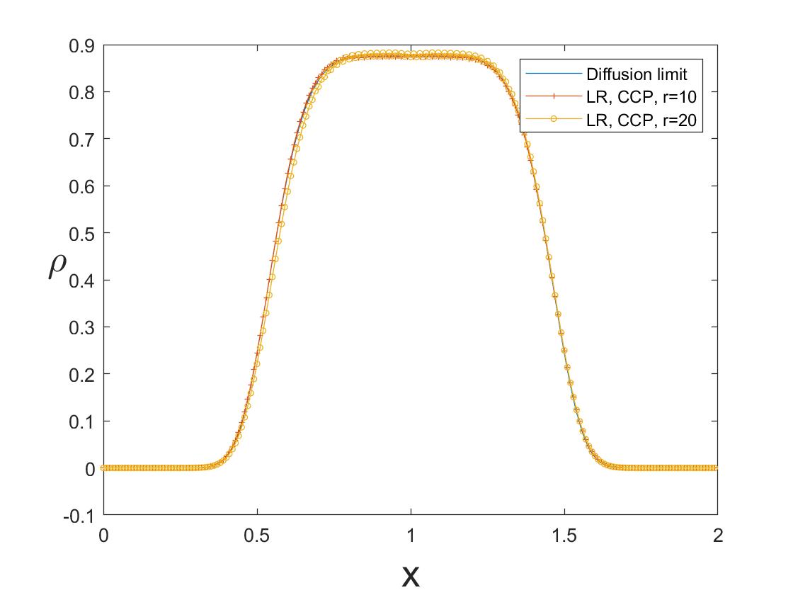
Refer to caption
(a)
Refer to caption
(b)
Figure 4: Example II\mathrm{II}. Nx=200,Nv=100,Δ​t=Δ​t2=Δ​x/3,Δ​t1=(Δ​t2)2N_{x}=200,N_{v}=100,\Delta t=\Delta t_{2}=\Delta x/3,\Delta t_{1}=(\Delta t_{2})^{2}. Left: ϵ=1\epsilon=1 and r=10,20r=10,20, we compare the density ρ\rho from the low-rank algorithm using CCP for 𝖣k\mathsf{D}_{k} with the implicit Euler/upwind solver at tmax=1t_{\text{max}}=1. Right: ϵ=10−3\epsilon=10^{-3} and r=10,20r=10,20, we compare the density ρ\rho from the low-rank algorithm using CCP with the diffusion limit at tmax=0.1t_{\text{max}}=0.1. In the plots, LR stands for dynamical low-rank solution.
Refer to caption
(a)
Refer to caption
(b)
Figure 5: Example II\mathrm{II}. Nx=200,Nv=100,Δ​t=Δ​t2=Δ​x/3,Δ​t1=(Δ​t2)2,r=20N_{x}=200,N_{v}=100,\Delta t=\Delta t_{2}=\Delta x/3,\Delta t_{1}=(\Delta t_{2})^{2},r=20. The numerical solution uu is computed using the implicit Euler/upwind solver and 𝖷,𝖵\mathsf{X},\mathsf{V} is computed using the low-rank algorithm. Left: log⁡(𝒫x,le​r​r​o​r‖u‖F)\log\left(\frac{\mathcal{P}^{error}_{x,l}}{\|u\|_{F}}\right) as a function of ll. Right: log⁡(𝒫v,le​r​r​o​r‖u‖F)\log\left(\frac{\mathcal{P}^{error}_{v,l}}{\|u\|_{F}}\right) as a function of ll.
Refer to caption
(a)
Refer to caption
(b)
Figure 6: Example II\mathrm{II}. Nx=200,Nv=100,Δ​t=Δ​t2=Δ​x/3,Δ​t1=(Δ​t2)2N_{x}=200,N_{v}=100,\Delta t=\Delta t_{2}=\Delta x/3,\Delta t_{1}=(\Delta t_{2})^{2}. Left: ϵ=1\epsilon=1 and r=10,20r=10,20, we compare the density ρ\rho from the low-rank algorithm using upwind and central differences for 𝖣k\mathsf{D}_{k} with the implicit Euler/upwind solver at tmax=1t_{\text{max}}=1. Right: ϵ=10−3\epsilon=10^{-3} and r=20r=20, we compare the density ρ\rho from the low-rank algorithm using central differences with the diffusion limit at tmax=0.1t_{\text{max}}=0.1. In the plots, LR stands for dynamical low-rank solution, and CS stands for central scheme, while UP stands for upwinding.

4.4 Example III\mathrm{III}

In the third example, we use the same initial condition as in Example II\mathrm{II}, but modify the cross section:

σ(x)={ 0.02,x∈[0.35,0.65]∪[1.35,1.65], 1,x∈[0,0.35)∪(0.65,1.35)∪(1.65,2].\sigma(x)=\left\{\begin{aligned} &\ 0.02,\quad x\in[0.35,0.65]\cup[1.35,1.65]\,,\\ &\ 1,\quad x\in[0,0.35)\cup(0.65,1.35)\cup(1.65,2]\,.\end{aligned}\right. (63)

This cross section is of high contrast and has a discontinuity, and thus the equation quickly achieves equilibrium in the optical thick region (σ∼1\sigma\sim 1), while still staying in the kinetic regime in the optical thin region (σ∼0.02\sigma\sim 0.02). The dynamical low-rank integrator uses r=20r=20. To obtain the reference solutions, we either compute the equation with fine grid when ϵ=1\epsilon=1, or compute the diffusion equation directly with ϵ=10−3\epsilon=10^{-3}. We also compute the error: it decays exponentially fast, as plotted in Figure 8.

Refer to caption
(a)
Refer to caption
(b)
Figure 7: Example III\mathrm{III}. Nx=200,Nv=100,Δ​t=Δ​t2=Δ​x/3,Δ​t1=(Δ​t2)2N_{x}=200,N_{v}=100,\Delta t=\Delta t_{2}=\Delta x/3,\Delta t_{1}=(\Delta t_{2})^{2}. Left: ϵ=1\epsilon=1 and r=10,20r=10,20, we compare the density ρ\rho from the low-rank algorithm using CCP for 𝖣k\mathsf{D}_{k} with the implicit Euler/upwind solver at tmax=1t_{\text{max}}=1. Right: ϵ=10−3\epsilon=10^{-3} and r=10,20r=10,20, we compare the density ρ\rho from the low-rank algorithm using CCP with the diffusion limit at tmax=0.1t_{\text{max}}=0.1.
Refer to caption
(a)
Refer to caption
(b)
Figure 8: Example III\mathrm{III}. Here we use Nx=200,Nv=100,Δ​t=Δ​t2=Δ​x/3,Δ​t1=(Δ​t2)2,r=20N_{x}=200,N_{v}=100,\Delta t=\Delta t_{2}=\Delta x/3,\Delta t_{1}=(\Delta t_{2})^{2},r=20. the numerical solution uu is computed using the implicit Euler/upwind solver and 𝖷,𝖵\mathsf{X},\mathsf{V} is computed using the low-rank algorithm. Left: log⁡(𝒫x,le​r​r​o​r‖u‖F)\log\left(\frac{\mathcal{P}^{error}_{x,l}}{\|u\|_{F}}\right) as a function of ll. Right: log⁡(𝒫v,le​r​r​o​r‖u‖F)\log\left(\frac{\mathcal{P}^{error}_{v,l}}{\|u\|_{F}}\right) as a function of ll.

5 Conclusion

We have applied a projector splitting based dynamical low-rank approximation to a multi-scale linear Boltzmann equation in diffusive scaling. Theoretically the equation has a low rank structure in this regime, and this paper studies if the dynamical low-rank numerical method, a highly nonlinear numerical method, can capture such structure.

The result crucially depends on the employed time integrator. As shown above, if the implicit Euler method is employed, the time stepsize needs to be small. However, the CNIE method, due to its embedded symmetry, can preserve the low rank structure automatically for mild time stepsize requirements, if the initial data is well-prepared. Combining these conclusions, we propose to run the Euler method for a very small time stepsize for merely one step to enforce the low rank structure, and then switch to CNIE to preserve the rank structure. Numerical evidence is shown to agrees well with the theoretical results obtained.

To our knowledge, this is the first analytical result on showing that the project-splitting dynamical low-rank approximation method truly preserves the rank structure in the kinetic framework.

Acknowledgement. The work of QL is supported in part by National Science Foundation under the grant DMS-1619778, and RNMS KI-NET 1107291. The work of ZD is supported in part by Wisconsin Data Science Initiative, and National Science Foundation under the grant DMS-1750488 and TRIPODS: 1740707.

References

  • [1] A. Arnold and T. Jahnke. On the approximation of high-dimensional differential equations in the hierarchical Tucker format. BIT Numer. Math., 54(2):305–341, 2014.
  • [2] C. Bardos, R. Santos, and R Sentis. Diffusion approximation and computation of the critical size. Trans. Amer. Math. Soc., 284(2):617–649, 1984.
  • [3] M. Bennoune, M. Lemou, and L. Mieussens. Uniformly stable numerical schemes for the Boltzmann equation preserving the compressible Navier-Stokes asymptotics. J. Comput. Phys., 227:3781–3803, 2008.
  • [4] D. Conte and C. Lubich. An error analysis of the multi-configuration time-dependent Hartree method of quantum dynamics. ESAIM Math. Model. Numer. Anal., 44(4):759–780, 2010.
  • [5] N. Crouseilles, M. Mehrenberger, and F. Vecil. Discontinuous Galerkin semi-Lagrangian method for Vlasov-Poisson. In ESAIM: Proceedings, volume 32, pages 211–230, 2011.
  • [6] W. Dahmen, R. DeVore, L. Grasedyck, and E. Süli. Tensor-sparsity of solutions to high-dimensional elliptic partial differential equations. Found. Comput. Math., 16(4):813–874, 2016.
  • [7] P. Degond, F. Deluzet, L. Navoret, A. Sun, and M. Vignal. Asymptotic-preserving particle-in-cell method for the vlasov–poisson system near quasineutrality. Journal of Computational Physics, 229(16):5630 – 5652, 2010.
  • [8] P. Degond, S. Jin, and J. Liu. Mach-number uniform asymptotic-preserving gauge schemes for compressible flows. Bull. Inst. Math. Acad. Sin. (N.S.), 2, 01 2007.
  • [9] G. Dimarco and L. Pareschi. Exponential Runge-Kutta methods for stiff kinetic equations. SIAM Journal on Numerical Analysis, 49(1):2057–2077, 2011.
  • [10] G. Dimarco and L. Pareschi. Numerical methods for kinetic equations. Acta Numer., 23:369–520, 2014.
  • [11] L. Einkemmer. A low-rank algorithm for weakly compressible flow. arXiv:1804.04561.
  • [12] L. Einkemmer. High performance computing aspects of a dimension independent semi-Lagrangian discontinuous Galerkin code. Comput. Phys. Commun., 202:326–336, 2016.
  • [13] L. Einkemmer. A performance comparison of semi-Lagrangian discontinuous Galerkin and spline based Vlasov solvers in four dimensions. J. Comput. Phys., 376:937–951, 2019.
  • [14] L. Einkemmer and C. Lubich. A low-rank projector-splitting integrator for the Vlasov–Poisson equation. SIAM J. Sci. Comput., 40:B1330–B1360, 2018.
  • [15] L. Einkemmer and C. Lubich. A quasi-conservative dynamical low-rank algorithm for the vlasov equation. SIAM Journal on Scientific Computing, 41(5):B1061–B1081, 2019.
  • [16] L. Einkemmer, A. Ostermann, and C. Piazzola. A low-rank projector-splitting integrator for the Vlasov–Maxwell equations with divergence correction. arXiv:1902.00424, 2019.
  • [17] F. Filbet and E. Sonnendrücker. Comparison of Eulerian Vlasov solvers. Comput. Phys. Commun., 150(3):247–266, 2003.
  • [18] V. Grandgirard, J. Abiteboul, J. Bigot, T. Cartier-Michaud, N. Crouseilles, G. Dif-Pradalier, Ch. Ehrlacher, D. Esteve, X. Garbet, Ph. Ghendrih, G. Latu, M. Mehrenberger, C. Norscini, C. Passeron, F. Rozar, Y. Sarazin, E. Sonnendrücker, A. Strugarek, and D. Zarzoso. A 5D gyrokinetic full-f global semi-Lagrangian code for flux-driven ion turbulence simulations. Comput. Phys. Commun., 207:35–68, 2016.
  • [19] J. Haegeman, C. Lubich, I. Oseledets, B. Vandereycken, and F. Verstraete. Unifying time evolution and optimization with matrix product states. Physical Review B, 94(16):165116, 2016.
  • [20] J. Hu, S. Jin, and Q. Li. Chapter 5 - Asymptotic-Preserving Schemes for Multiscale Hyperbolic and Kinetic Equations. In R. Abgrall and C. Shu, editors, Handbook of Numerical Methods for Hyperbolic Problems, volume 18 of Handbook of Numerical Analysis, pages 103 – 129. Elsevier, 2017.
  • [21] S. Jin. Efficient Asymptotic-Preserving (AP) Schemes For Some Multiscale Kinetic Equations. SIAM J. Sci. Comput., 21(2):441–454, 1999.
  • [22] S. Jin and C.D. Levermore. Numerical Schemes for Hyperbolic Conservation Laws with Stiff Relaxation Terms. J. Comput. Phys., 126(2):449 – 467, 1996.
  • [23] S. Jin and L. Pareschi. Asymptotic-Preserving (AP) Schemes for Multiscale Kinetic Equations: a Unified Approach. In H. Freistühler and G. Warnecke, editors, Hyperbolic Problems: Theory, Numerics, Applications, pages 573–582. Birkhäuser Basel, Basel, 2001.
  • [24] S. Jin, L. Pareschi, and G. Toscani. Uniformly accurate diffusive relaxation schemes for multiscale transport equations. SIAM J. Numer. Anal., 38(3):913–936, 2000.
  • [25] E. Kieri, C. Lubich, and H. Walach. Discretized dynamical low-rank approximation in the presence of small singular values. SIAM J. Numer. Anal., 54(2):1020–1038, 2016.
  • [26] O. Koch and C. Lubich. Dynamical low-rank approximation. SIAM J. Matrix Anal. Appl., 29(2):434–454, 2007.
  • [27] O. Koch and C. Lubich. Dynamical tensor approximation. SIAM J. Matrix Anal. Appl., 31(5):2360–2375, 2010.
  • [28] K. Kormann. A semi-Lagrangian Vlasov solver in tensor train format. SIAM J. Sci. Comput., 37(4):613–632, 2015.
  • [29] E. Larsen, J. Morel, and W. Miller. Asymptotic solutions of numerical transport problems in optically thick, diffusive regimes. J. Comput. Phys., 69(2):283 – 324, 1987.
  • [30] M. Lemou and L. Mieussens. A new asymptotic preserving scheme based on micro-macro formulation for linear kinetic equations in the diffusion limit. SIAM J. Sci. Comput., 31:334–368, 2008.
  • [31] Q. Li, J. Lu, and W. Sun. A convergent method for linear half-space kinetic equations. ESAIM: Mathematical Modelling and Numerical Analysis, 51(5):1583–1615, 2017.
  • [32] Q. Li, J. Lu, and W. Sun. Half-space kinetic equations with general boundary conditions. Math. Comp., 86:1269–1301, 2017.
  • [33] Q. Li, J. Lu, and W. Sun. Validity and regularization of classical half-space equations. Journal of Statistical Physics, 166(2):398–433, 2017.
  • [34] Q. Li and L. Pareschi. Exponential Runge-Kutta for the inhomogeneous Boltzmann equations with high order of accuracy. J. Comput. Phys., 259:402–420, 2014.
  • [35] Q. Li and L. Wang. Implicit Asymptotic Preserving Method for Linear Transport Equations. Commun. Comput. Phys., 22(1):157–181, 2017.
  • [36] C. Lubich. From quantum to classical molecular dynamics: reduced models and numerical analysis. European Mathematical Society, 2008.
  • [37] C. Lubich. Time integration in the multiconfiguration time-dependent Hartree method of molecular quantum dynamics. Applied Mathematics Research eXpress, 2015(2):311–328, 2015.
  • [38] C. Lubich, I. V. Oseledets, and B. Vandereycken. Time integration of tensor trains. SIAM J. Numer. Anal., 53(2):917–941, 2015.
  • [39] C. Lubich and I.V. Oseledets. A projector-splitting integrator for dynamical low-rank approximation. BIT Numer. Math., 54(1):171–188, 2014.
  • [40] C. Lubich, T. Rohwedder, R. Schneider, and B. Vandereycken. Dynamical approximation by hierarchical Tucker and tensor-train tensors. SIAM J. Matrix Anal. Appl., 34(2):470–494, 2013.
  • [41] C. Lubich, B. Vandereycken, and H. Walach. Time integration of rank-constrained tucker tensors. SIAM J. Numer. Anal., 56(3):1273–1290, 2018.
  • [42] H. Meyer, F. Gatti, and G. A. Worth. Multidimensional quantum dynamics. John Wiley & Sons, 2009.
  • [43] H. Meyer, U. Manthe, and L. S. Cederbaum. The multi-configurational time-dependent Hartree approach. Chem. Phys. Letters, 165(1):73–78, 1990.
  • [44] C. Mouhot and C. Villani. On landau damping. Acta Math., 207(1):29–201, Sep 2011.
  • [45] A. Nonnenmacher and C. Lubich. Dynamical low-rank approximation: applications and numerical experiments. Math. Comput. Simul., 79(4):1346 – 1357, 2008.
  • [46] A. Ostermann, C. Piazzola, and H. Walach. Convergence of a low-rank lie–trotter splitting for stiff matrix differential equations. SIAM Journal on Numerical Analysis, 57(4):1947–1966, 2019.
  • [47] N. J. Sircombe and T. D. Arber. VALIS: A split-conservative scheme for the relativistic 2D Vlasov–Maxwell system. J. Comput. Phys., 228(13):4773–4788, 2009.
  • [48] D. Ter Haar. Men of physics: L.D. Landau, volume 2. Elsevier, 1969.
  • [49] L. Wu and Y. Guo. Geometric correction for diffusive expansion of steady neutron transport equation. Communications in Mathematical Physics, 336(3):1473–1553, 2015.

Appendix A Details for the proof of Theorem 4

Lemma 5.

If Assumption 1 holds true, then for all n>0n>0, 𝖫0n\mathsf{L}^{n}_{0} and 𝖲0n+1/3\mathsf{S}^{n+1/3}_{0} can be written as follows

𝖫0n=l0n​en⊤,𝖲0n+1/3=s0n+1/3​(αn+1)⊤,αn+1=𝖵n+1​en⊤,\mathsf{L}^{n}_{0}=l^{n}_{0}e^{\top}_{\mathrm{n}},\quad\mathsf{S}^{n+1/3}_{0}=s^{n+1/3}_{0}\left(\alpha^{n+1}\right)^{\top},\quad\alpha^{n+1}=\mathsf{V}^{n+1}e^{\top}_{\mathrm{n}}, (64)

with some l0n∈ℝr×1l^{n}_{0}\in\mathbb{R}^{r\times 1} and s0n+1/3∈ℝr×1s^{n+1/3}_{0}\in\mathbb{R}^{r\times 1}.

Remark 9.

Using Assumption 1 and Lemma 5, we can further prove that in each step, 𝖫n+1/3\mathsf{L}^{n+1/3} can be written as

𝖫n+1/3=l^n+1/3​en⊤−ϵ​∑k=1d(Aσn)−1​A∂kn​l^n+1/3​en⊤​Πvk+O⁡(ϵ2),\mathsf{L}^{n+1/3}=\hat{l}^{n+1/3}e^{\top}_{\mathrm{n}}-\epsilon\sum^{d}_{k=1}(A^{n}_{\sigma})^{-1}A^{n}_{\partial_{k}}\hat{l}^{n+1/3}e^{\top}_{\mathrm{n}}\mathsf{\Pi}_{v_{k}}+O(\epsilon^{2}), (65)

where l^n+1/3=l0n+1/3+ϵ​l1n+1/3\hat{l}^{n+1/3}=l^{n+1/3}_{0}+\epsilon l^{n+1/3}_{1}.

Proof.

The proof proceeds by induction. First, for n=1n=1, by (52), after doing QR decomposition, we obtain

𝖲01=s1​e1,r​(α1)⊤,e1,r=(1,0,…,0)⊤∈ℝr×1,\mathsf{S}^{1}_{0}=s^{1}e_{1,r}(\alpha^{1})^{\top},\quad e_{1,r}=\left(1,0,\dots,0\right)^{\top}\in\mathbb{R}^{r\times 1}, (66)

where s1∈ℝs^{1}\in\mathbb{R} and α1=(𝖵1)⊤​en\alpha^{1}=(\mathsf{V}^{1})^{\top}e_{\mathrm{n}}. Using Assumption 1, we then get

𝖫01=s1​e1,r​(α1)⊤​(𝖵1)⊤+O⁡(ϵ)=s1​e1,r​(α1,∗)⊤​(𝖵1,∗)⊤+O⁡(ϵ)=s1​e1,r​en⊤+O⁡(ϵ)\mathsf{L}^{1}_{0}=s^{1}e_{1,r}(\alpha^{1})^{\top}(\mathsf{V}^{1})^{\top}+O(\epsilon)=s^{1}e_{1,r}(\alpha^{1,*})^{\top}(\mathsf{V}^{1,*})^{\top}+O(\epsilon)=s^{1}e_{1,r}e^{\top}_{\mathrm{n}}+O(\epsilon) (67)

Let l01=s1​e1,rl^{1}_{0}=s^{1}e_{1,r}, if we consider terms of order O⁡(1/ϵ)O(1/\epsilon) in the asymptotic expansion of equation (23), we obtain

𝖫04/3+𝖫01=l04/3​en⊤+l01​en⊤.\mathsf{L}^{4/3}_{0}+\mathsf{L}^{1}_{0}=l^{4/3}_{0}e^{\top}_{\mathrm{n}}+l^{1}_{0}e^{\top}_{\mathrm{n}}. (68)

After performing the QR decomposition we have

𝖲04/3=𝖫0n+1/3​𝖵2+O⁡(ϵ)=l04/3​en⊤​𝖵2+O⁡(ϵ)=l04/3​(α2)⊤+O⁡(ϵ).\mathsf{S}^{4/3}_{0}=\mathsf{L}^{n+1/3}_{0}\mathsf{V}^{2}+O(\epsilon)=l^{4/3}_{0}e^{\top}_{\mathrm{n}}\mathsf{V}^{2}+O(\epsilon)=l^{4/3}_{0}\left(\alpha^{2}\right)^{\top}+O(\epsilon). (69)

This shows that equation (64) holds true for n=1n=1.

Now if for n=k−1n=k-1 equation (64) holds true, then we can show that

𝖫0k=l0k​en⊤,\mathsf{L}^{k}_{0}=l^{k}_{0}e^{\top}_{\mathrm{n}}, (70)

which implies

𝖫0k+1/3+𝖫0k=l0k+1/3​en⊤+l0k​en⊤.\mathsf{L}^{k+1/3}_{0}+\mathsf{L}^{k}_{0}=l^{k+1/3}_{0}e^{\top}_{\mathrm{n}}+l^{k}_{0}e^{\top}_{\mathrm{n}}. (71)

Then we perform a QR decomposition and obtain

𝖲0k+1/3=s0k+1/3​(αn+1)⊤,\mathsf{S}^{k+1/3}_{0}=s^{k+1/3}_{0}\left(\alpha^{n+1}\right)^{\top}, (72)

where s0k+1/3=l0k+1/3s^{k+1/3}_{0}=l^{k+1/3}_{0}.

We now, consider the proof of Theorem 4 in more detail.

Proof.

Step 1-2: Instead of (45) and (49). We can obtain

u0n+1/3​e−u0n​eΔ​t−1d​∑k=1d𝖷n​𝖠∂kn​(𝖠σn)−1​𝖠∂kn​(𝖷n)⊤​u0n+1/3​e+u0n​e2=0,\frac{u^{n+1/3}_{0}e-u^{n}_{0}e}{\Delta t}-\frac{1}{d}\sum^{d}_{k=1}\mathsf{X}^{n}\mathsf{A}^{n}_{\partial_{k}}(\mathsf{A}^{n}_{\sigma})^{-1}\mathsf{A}^{n}_{\partial_{k}}(\mathsf{X}^{n})^{\top}\frac{u^{n+1/3}_{0}e+u^{n}_{0}e}{2}=0, (73)
u0n+2/3​e−u0n+1/3​eΔ​t+1d​∑k=1d𝖷n​𝖠∂kn​(𝖠σn)−1​𝖠∂kn​(𝖷n)⊤​u0n+2/3​e+u0n+1/3​e2=0\frac{u^{n+2/3}_{0}e-u^{n+1/3}_{0}e}{\Delta t}+\frac{1}{d}\sum^{d}_{k=1}\mathsf{X}^{n}\mathsf{A}^{n}_{\partial_{k}}(\mathsf{A}^{n}_{\sigma})^{-1}\mathsf{A}^{n}_{\partial_{k}}(\mathsf{X}^{n})^{\top}\frac{u^{n+2/3}_{0}e+u^{n+1/3}_{0}e}{2}=0 (74)

This gives us

ρ0n+1/3=(I−(Δ​t)2​d​ℒn)−1​(I+(Δ​t)2​d​ℒn)​ρ0n,\displaystyle\rho^{n+1/3}_{0}=\left(I-\frac{(\Delta t)}{2d}\mathcal{L}^{n}\right)^{-1}\left(I+\frac{(\Delta t)}{2d}\mathcal{L}^{n}\right)\rho^{n}_{0}, (75)
ρ0n+2/3=(I+(Δ​t)2​d​ℒn)−1​(I−(Δ​t)2​d​ℒn)​ρ0n+1/3\displaystyle\rho^{n+2/3}_{0}=\left(I+\frac{(\Delta t)}{2d}\mathcal{L}^{n}\right)^{-1}\left(I-\frac{(\Delta t)}{2d}\mathcal{L}^{n}\right)\rho^{n+1/3}_{0} (76)
⇒\displaystyle\Rightarrow ρ0n+2/3=ρ0n.\displaystyle\rho^{n+2/3}_{0}=\rho^{n}_{0}. (77)

Now, we obtain

ρ0n+2/3=ρ0n,for​n>0.\rho^{n+2/3}_{0}=\rho^{n}_{0},\quad\text{for}\ n>0. (78)

in the first two splitting step with CNIE scheme.

Step 3: Using equation (64) we have

𝖲0n+1/3=s0n+1/3​(αn+1)⊤.\mathsf{S}^{n+1/3}_{0}=s^{n+1/3}_{0}\left(\alpha^{n+1}\right)^{\top}. (79)

From the terms of order O⁡(1/ϵ)O(1/\epsilon) we then obtain

𝖲0n+2/3=s0n+2/3​(αn+1)⊤⇒𝖪0n+2/3=k0n+2/3​(αn+1)⊤.\mathsf{S}^{n+2/3}_{0}=s^{n+2/3}_{0}\left(\alpha^{n+1}\right)^{\top}\Rightarrow\mathsf{K}^{n+2/3}_{0}=k^{n+2/3}_{0}\left(\alpha^{n+1}\right)^{\top}. (80)

Repeating the procedure used to derive equations (53)-(54), we still recover the diffusion limit in the last splitting step as

ρ0n+1−ρ0n+2/3Δ​t−1d​∑k=1d𝖣k​(Σ−1​𝖣k​ρ0n+1)=0.\frac{\rho^{n+1}_{0}-\rho_{0}^{n+2/3}}{\Delta t}-\frac{1}{d}\sum^{d}_{k=1}\mathsf{D}_{{k}}\left(\mathsf{\Sigma}^{-1}\mathsf{D}_{{k}}\rho^{n+1}_{0}\right)=0. (81)

Appendix B Discussion on the technical assumption

We first note that conditions (33),(34) in Assumption 1 guarantee the orthonormality of V1,∗V^{1,*}. Now, using equation (34) and denoting αn+1,∗=𝖰⊤​αn+1\alpha^{n+1,*}=\mathsf{Q}^{\top}\alpha^{n+1} we have

αn+1,∗​(αn+1,∗)⊤=𝖰⊤​αn+1​(αn+1)⊤​𝖰,(αn+1,∗)⊤​αn+1,∗=(αn+1)⊤​αn+1=1+O⁡(ϵ4).\alpha^{n+1,\ast}(\alpha^{n+1,\ast})^{\top}=\mathsf{Q}^{\top}\alpha^{n+1}(\alpha^{n+1})^{\top}\mathsf{Q},\ (\alpha^{n+1,\ast})^{\top}\alpha^{n+1,\ast}=(\alpha^{n+1})^{\top}\alpha^{n+1}=1+O(\epsilon^{4}). (82)

For each 1≤k≤d1\leq k\leq d, we define

Ξvkn+1,∗=(𝖵n+1,∗)⊤​d​i​a​g​(𝒱k)​𝖵n+1,∗,\mathsf{\Xi}^{n+1,\ast}_{v_{k}}=(\mathsf{V}^{n+1,\ast})^{\top}diag(\mathcal{V}_{k})\mathsf{V}^{n+1,\ast}\,,

then we get

Ξvkn+1,∗=𝖰⊤​Ξvkn+1​𝖰,(Ξvkn+1,∗)1,j=(Ξvkn+1,∗)j,1=1d​δk+1,j+O⁡(ϵ),1≤j≤Nv,\mathsf{\Xi}^{n+1,\ast}_{v_{k}}=\mathsf{Q}^{\top}\mathsf{\Xi}^{n+1}_{v_{k}}\mathsf{Q},\quad\left(\mathsf{\Xi}^{n+1,\ast}_{v_{k}}\right)_{1,j}=\left(\mathsf{\Xi}^{n+1,\ast}_{v_{k}}\right)_{j,1}=\frac{1}{\sqrt{d}}\delta_{k+1,j}+O(\epsilon),\quad 1\leq j\leq N_{v}, (83)

where the second equality can be shown by using equation (34).

By considering equations (44) and (65), it suffices to show that the space spanned by the rows of l0n+1/3​en⊤−ϵ​∑i=1d(𝖠σn)−1​𝖠∂in​l0n+1/3​en⊤​Πvil^{n+1/3}_{0}e^{\top}_{\mathrm{n}}-\epsilon\sum^{d}_{i=1}(\mathsf{A}^{n}_{\sigma})^{-1}\mathsf{A}^{n}_{\partial_{i}}l^{n+1/3}_{0}e^{\top}_{\mathrm{n}}\mathsf{\Pi}_{v_{i}} can contain en⊤,𝒱1⊤,…,𝒱d⊤e^{\top}_{\mathrm{n}},\mathcal{V}^{\top}_{1},\dots,\mathcal{V}^{\top}_{d}. This, in turn, is equivalent to show that the following ℝr×(d+1)\mathbb{R}^{r\times(d+1)} matrix has at least rank d+1d+1

ℛ=(𝖠σn​l0n+1/3,𝖠∂1n​l0n+1/3,⋯,𝖠∂dn​l0n+1/3).\mathcal{R}=\left(\mathsf{A}^{n}_{\sigma}l^{n+1/3}_{0},\mathsf{A}^{n}_{\partial_{1}}l^{n+1/3}_{0},\cdots,\mathsf{A}^{n}_{\partial_{d}}l^{n+1/3}_{0}\right). (84)

For convenience, we only consider σ⁡(x)=1\sigma(x)=1 and 𝖣i\mathsf{D}_{i} is skew-symmetric.

First, we define the operator ℋ:ℝNx×1→ℝd×d\mathcal{H}:\mathbb{R}^{N_{x}\times 1}\rightarrow\mathbb{R}^{d\times d} as follows

(ℋ⁡(k))i,j=(𝖣i​k)⊤​(𝖣j​k),k∈ℝNx×1\left(\mathcal{H}(\textbf{k})\right)_{i,j}=\left(\mathsf{D}_{i}\textbf{k}\right)^{\top}\left(\mathsf{D}_{j}\textbf{k}\right),\quad\textbf{k}\in\mathbb{R}^{N_{x}\times 1} (85)
Lemma 6.

Assume Assumption 1 is true for the numerical solution at time tnt_{n}, Δ​t(Δ​x)2\frac{\Delta t}{(\Delta x)^{2}} and ϵ\epsilon are small enough, if

d​e​t​(ℋ⁡(kn))≠0,det(\mathcal{H}(k^{n}))\neq 0, (86)

where knk^{n} is defined in equation (52), then Assumption 1 is true for the numerical solution at time tn+1t_{n+1}.

Remark 10.

By Lemma 6, we only need to check condition (86). Since knk^{n} is a discrete approximation to ρ⁡(x,tn)\rho(x,t^{n}), assume numerical error is small and the solution satisfies

D⁡(ρ)​(t)=d​e​t​(∫Ωx∇ρ​(x,t)​(∇ρ​(x,t))⊤​𝑑x)≠0,∀0≤t≤T,D(\rho)(t)=det\left(\int_{\Omega_{x}}\nabla\rho(x,t)\left(\nabla\rho(x,t)\right)^{\top}dx\right)\neq 0,\quad\forall 0\leq t\leq T,

then we have ℋ⁡(kn)≈D⁡(ρ)​(tn)\mathcal{H}(k^{n})\approx D(\rho)(t^{n}) and (86).

Proof.

If Assumption 1 is true at time tn−1t_{n-1}, we have

𝖪n=kn​(αn)⊤−ϵ​∑i=1d𝖣i​kn​(αn)⊤​Ξvin+O⁡(ϵ2).\mathsf{K}^{n}=k^{n}\left(\alpha^{n}\right)^{\top}-\epsilon\sum^{d}_{i=1}\mathsf{D}_{i}k^{n}\left(\alpha^{n}\right)^{\top}\mathsf{\Xi}^{n}_{v_{i}}+O(\epsilon^{2}).

and there exists an orthogonal matrix 𝖰\mathsf{Q} such that

𝖪n​𝖰=kn​(αn,∗)⊤−ϵ​∑i=1d𝖣i​kn​(αn,∗)⊤​Ξvin,∗+O⁡(ϵ2),\mathsf{K}^{n}\mathsf{Q}=k^{n}\left(\alpha^{n,*}\right)^{\top}-\epsilon\sum^{d}_{i=1}\mathsf{D}_{i}k^{n}\left(\alpha^{n,*}\right)^{\top}\mathsf{\Xi}^{n,*}_{v_{i}}+O(\epsilon^{2}), (87)

where αn,∗\alpha^{n,*}, Ξvin,∗\mathsf{\Xi}^{n,*}_{v_{i}} satisfy (82) and (83).

Use (82) and (83), we can rewrite (87) as

𝖪n𝖰=(kn,−ϵd𝖣1kn,…,−ϵd𝖣dkn,…,)+O(ϵ2).\mathsf{K}^{n}\mathsf{Q}=\left(k^{n},-\frac{\epsilon}{\sqrt{d}}\mathsf{D}_{1}k^{n},\dots,-\frac{\epsilon}{\sqrt{d}}\mathsf{D}_{d}k^{n},\dots,\right)+O(\epsilon^{2}). (88)

We notice that 𝖷n\mathsf{X}^{n} comes from QR decomposition of 𝖪n−1\mathsf{K}^{n-1}. Therefore, use (88), there exits an invertible matrix 𝖯∈ℝr×r\mathsf{P}\in\mathbb{R}^{r\times r} such that

𝖷∗=𝖷n𝖯−1=(kn,−𝖣1kn,…,−𝖣dkn,…,)+O(ϵ).\mathsf{X}^{*}=\mathsf{X}^{n}\mathsf{P}^{-1}=\left(k^{n},-\mathsf{D}_{1}k^{n},\dots,-\mathsf{D}_{d}k^{n},\dots,\right)+O(\epsilon). (89)

For any 1≤i≤d1\leq i\leq d, we further define

𝖠∂i∗=(𝖷∗)⊤​𝖣i​𝖷∗,then​𝖠∂in=𝖯⊤​𝖠∂i∗​𝖯\mathsf{A}^{*}_{\partial_{i}}=\left(\mathsf{X}^{*}\right)^{\top}\mathsf{D}_{i}\mathsf{X}^{*},\ \text{then}\ \mathsf{A}^{n}_{\partial_{i}}=\mathsf{P}^{\top}\mathsf{A}^{*}_{\partial_{i}}\mathsf{P} (90)

and

𝖠σ∗=(𝖷∗)⊤​Σ​𝖷∗,then​𝖠σn=𝖯⊤​𝖠σ∗​𝖯.\mathsf{A}^{*}_{\sigma}=\left(\mathsf{X}^{*}\right)^{\top}\mathsf{\Sigma}\mathsf{X}^{*},\ \text{then}\ \mathsf{A}^{n}_{\sigma}=\mathsf{P}^{\top}\mathsf{A}^{*}_{\sigma}\mathsf{P}. (91)

Plug equations (90),(91) into (84) and define l∗=𝖯​l0n+1/3l^{*}=\mathsf{P}l^{n+1/3}_{0}, it suffices to show that

ℛ∗=(𝖠σ∗​l∗,𝖠∂1∗​l∗,⋯,𝖠∂d∗​l∗)\mathcal{R}^{*}=\left(\mathsf{A}^{*}_{\sigma}l^{*},\mathsf{A}^{*}_{\partial_{1}}l^{*},\cdots,\mathsf{A}^{*}_{\partial_{d}}l^{*}\right)

has rank d+1d+1. Now we divide the following proof into two steps:

First step: (l∗)1≫0(l^{*})_{1}\gg 0. Similar to equation (70), we have

𝖲n​(𝖵n)⊤=𝖫n=l0n​en⊤+O⁡(ϵ).\mathsf{S}^{n}\left(\mathsf{V}^{n}\right)^{\top}=\mathsf{L}^{n}=l^{n}_{0}e^{\top}_{\mathrm{n}}+O(\epsilon).

Using (32),(52),(82), we get

𝖷∗​𝖯𝖲n​(𝖵n)⊤=𝖪n​(𝖵n)⊤=kn​(αn)⊤​(𝖵n)⊤=kn​(αn,∗)⊤​(𝖵n,∗)⊤=kn​en⊤+O⁡(ϵ2),\mathsf{X}^{*}\mathsf{P}\mathsf{S}^{n}\left(\mathsf{V}^{n}\right)^{\top}=\mathsf{K}^{n}\left(\mathsf{V}^{n}\right)^{\top}=k^{n}\left(\alpha^{n}\right)^{\top}\left(\mathsf{V}^{n}\right)^{\top}=k^{n}\left(\alpha^{n,*}\right)^{\top}\left(\mathsf{V}^{n,*}\right)^{\top}=k^{n}e^{\top}_{\mathrm{n}}+O(\epsilon^{2}),

which implies

𝖷∗​𝖯​l0n​en⊤=kn​en⊤.\mathsf{X}^{*}\mathsf{P}l^{n}_{0}e^{\top}_{\mathrm{n}}=k^{n}e^{\top}_{\mathrm{n}}.

Because 𝖷∗\mathsf{X}^{*} is an invertible matrix and the first column of 𝖷∗\mathsf{X}^{*} is knk^{n}, we must have

(𝖯​l0n)1=1+O⁡(ϵ).\left(\mathsf{P}l^{n}_{0}\right)_{1}=1+O(\epsilon). (92)

Recall that

(l∗)1=(𝖯​l0n+1/3)1,\left(l^{*}\right)_{1}=\left(\mathsf{P}l^{n+1/3}_{0}\right)_{1}, (93)

similar to asymptotic analysis performed to obtain (45), we have

𝖫0n+1/3​en−𝖫0n​enΔ​t−∑i=1d𝖠∂in​(𝖠σn)−1​𝖠∂in​l0n+1/3+l0n2​en⊤​Πvi2​en=0\displaystyle\frac{\mathsf{L}^{n+1/3}_{0}e_{\mathrm{n}}-\mathsf{L}^{n}_{0}e_{\mathrm{n}}}{\Delta t}-\sum^{d}_{i=1}\mathsf{A}^{n}_{\partial_{i}}(\mathsf{A}^{n}_{\sigma})^{-1}\mathsf{A}^{n}_{\partial_{i}}\frac{l^{n+1/3}_{0}+l^{n}_{0}}{2}e^{\top}_{\mathrm{n}}\mathsf{\Pi}^{2}_{v_{i}}e_{\mathrm{n}}=0
⇒\displaystyle\Rightarrow l0n+1/3−l0nΔ​t−1d​∑i=1d𝖠∂in​(𝖠σn)−1​𝖠∂in​l0n+1/3+l0n2=0,\displaystyle\frac{l^{n+1/3}_{0}-l^{n}_{0}}{\Delta t}-\frac{1}{d}\sum^{d}_{i=1}\mathsf{A}^{n}_{\partial_{i}}(\mathsf{A}^{n}_{\sigma})^{-1}\mathsf{A}^{n}_{\partial_{i}}\frac{l^{n+1/3}_{0}+l^{n}_{0}}{2}=0,

which implies

‖l0n+1/3−l0n‖2=O⁡(Δ​t(Δ​x)2).\|l^{n+1/3}_{0}-l^{n}_{0}\|_{2}=O\left(\frac{\Delta t}{(\Delta x)^{2}}\right). (94)

Combining (92),(93) with (94), we finally obtain

|(𝖯⁡(l0n+1/3−l0n))1|=O⁡(Δ​t(Δ​x)2)+O⁡(ϵ)⇒(l∗)1>1−[O⁡(Δ​t(Δ​x)2)+O⁡(ϵ)]≫0,\left|\left(\mathsf{P}\left(l^{n+1/3}_{0}-l^{n}_{0}\right)\right)_{1}\right|=O\left(\frac{\Delta t}{(\Delta x)^{2}}\right)+O(\epsilon)\Rightarrow\left(l^{*}\right)_{1}>1-\left[O\left(\frac{\Delta t}{(\Delta x)^{2}}\right)+O(\epsilon)\right]\gg 0,

where Δ​t(Δ​x)2\frac{\Delta t}{(\Delta x)^{2}}, ϵ\epsilon have to be very small.

Second step: Γ∗\Gamma^{*} is invertible. Now we can prove (86) by contradiction. If we assume there exists γ∈ℝ(d+1)×1\gamma\in\mathbb{R}^{(d+1)\times 1} with ‖γ‖2=1\|\gamma\|_{2}=1 such that

ℛ∗​γ=0⇒(𝖠σ∗​γ1+∑i=id𝖠∂i∗​γi+1)​l∗=0.\mathcal{R}^{*}\gamma=0\Rightarrow\left(\mathsf{A}^{*}_{\sigma}\gamma_{1}+\sum^{d}_{i=i}\mathsf{A}^{*}_{\partial_{i}}\gamma_{i+1}\right)l^{*}=0. (95)

Because 𝖣i\mathsf{D}_{i} is skew-symmetric, 𝖠∂i∗\mathsf{A}^{*}_{\partial_{i}} is skew-symmetric for each ii. From equation (95), we deduce

(l∗)⊤​(𝖠σ∗​γ1+∑i=id𝖠∂i∗​γi+1)​l∗=0⇒γ1​(l∗)⊤​𝖠σ∗​l∗=0⇒γ1=0⇒∑i=id𝖠∂i∗​l∗​γi+1=0,(l^{*})^{\top}\left(\mathsf{A}^{*}_{\sigma}\gamma_{1}+\sum^{d}_{i=i}\mathsf{A}^{*}_{\partial_{i}}\gamma_{i+1}\right)l^{*}=0\Rightarrow\gamma_{1}(l^{*})^{\top}\mathsf{A}^{*}_{\sigma}l^{*}=0\Rightarrow\gamma_{1}=0\Rightarrow\sum^{d}_{i=i}\mathsf{A}^{*}_{\partial_{i}}l^{*}\gamma_{i+1}=0,

where we use (l∗)⊤​𝖠∂i∗​l∗=0(l^{*})^{\top}\mathsf{A}^{*}_{\partial_{i}}l^{*}=0.

Plug equation (89) into equation (90), we obtain

(𝖠∂m∗)i,j={(𝖣i−1​kn)⊤​𝖣m​(𝖣j−1​kn),2≤i,j≤d+10,i=j−(𝖣i−1​kn)⊤​(𝖣m​kn)+O⁡(ϵ),2≤i≤d+1,j=1\left(\mathsf{A}^{*}_{\partial_{m}}\right)_{i,j}=\left\{\begin{aligned} &{\color[rgb]{0,0,0}{\left(\mathsf{D}_{i-1}k^{n}\right)^{\top}\mathsf{D}_{m}\left(\mathsf{D}_{j-1}k^{n}\right)}},\quad 2\leq i,j\leq d+1\\ &0,\quad i=j\\ &-\left(\mathsf{D}_{i-1}k^{n}\right)^{\top}\left(\mathsf{D}_{m}k^{n}\right)+O(\epsilon),\quad 2\leq i\leq d+1,\ j=1\end{aligned}\right. (96)

for any 1≤m≤d1\leq m\leq d. Consider the first column of 𝖠∂i∗\mathsf{A}^{*}_{\partial_{i}} from equation (96). Since (l∗)1≫0\left(l^{*}\right)_{1}\gg 0, equation (95) implies

ℋ(kn)γ(2:d+1)=0,\mathcal{H}(k^{n})\gamma_{(2:d+1)}=0,

where ℋ\mathcal{H} is defined in equation (85) and γ(2:d+1)∈ℝd×1\gamma_{(2:d+1)}\in\mathbb{R}^{d\times 1} is the cutoff vector to γ\gamma defined as

(γ(2:d+1))i=γi+1,1≤i≤d.\left(\gamma_{(2:d+1)}\right)_{i}=\gamma_{i+1},\quad 1\leq i\leq d\,.

Since ℋ⁡(kn)\mathcal{H}(k^{n}) is an invertible matrix, this finally shows that γ(2:d+1)\gamma_{(2:d+1)} has to be zero, which contradicts to ‖γ‖2=1\|\gamma\|_{2}=1.