Tensor -shrinkage nuclear norm for low-rank tensor completion
Abstract
In this paper, a new definition of tensor -shrinkage nuclear norm (-TNN) is proposed based on tensor singular value decomposition (t-SVD). In particular, it can be proved that -TNN is a better approximation of the tensor average rank than the tensor nuclear norm when . Therefore, by employing the -shrinkage nuclear norm, a novel low-rank tensor completion (LRTC) model is proposed to estimate a tensor from its partial observations. Statistically, the upper bound of recovery error is provided for the LRTC model. Furthermore, an efficient algorithm, accelerated by the adaptive momentum scheme, is developed to solve the resulting nonconvex optimization problem. It can be further guaranteed that the algorithm enjoys a global convergence rate under the smoothness assumption. Numerical experiments conducted on both synthetic and real-world data sets verify our results and demonstrate the superiority of our -TNN in LRTC problems over several state-of-the-art methods.
1 Introduction
In the fields of computer vision and signal processing, there are massive multi-dimensional data that needs to be analyzed and processed. In particular, multi-dimensional arrays (i.e., tensors) provide a natural representation form for these data. Tensor, which is regarded as a multi-linear generalization of matrix/vector, can mathematically model the multi-dimensional data structures, making tensor learning so attractive that there are increasing applications in computer vision [1, 2, 3, 4], machine learning [5, 6], signal processing [7, 8], and pattern recognition [9] in recent years. Unfortunately, the challenge of missing elements in the actually observed tensors limits its applications. Inspired by matrix completion [10], tensor completion attempts to recover the underlying tensor, that on the low-rank assumption, from its incomplete observations. Mathematically, the low-rank tensor completion (LRTC) problem can be formulated as the following model:
| (1) |
where denotes the underlying tensor and its observation tensor, respectively, denotes the rank function of , denotes the index set of observed entries, and denotes the projection operator that if and 0 otherwise. Different from matrix case, however, the definition of the tensor rank is not unique, and we can see that each definition corresponds to the particular tensor decomposition [11]. For example, tensor n-rank [12] is related to the Tucker decomposition [13], CP-rank [14] is related to the CANDECOMP/PARAFAC (CP) decomposition [15], tensor train (TT) rank is related to the TT decomposition [16], and tubal rank [2] and tensor multi-rank are related to tensor singular value decomposition (t-SVD) [17].
Due to the non-convex and non-smoothness of the rank function , the calculation of it is usually NP-hard problem that cannot be solved within polynomial time. Therefore, the function is usually relaxed as its convex/non-convex surrogate, and (1) can be rewritten as follows:
| (2) |
where denotes the surrogate function, denotes the regularization parameter, and denotes the smooth loss function. Obviously, the difference among the existing LRTC models mainly lies in the choice of . Although various tensor rank surrogates [3, 6, 18] are proposed to approximate the tensor rank, they all face some challenges in practical applications.
According to the CP decomposition [15], Friedland et al. [18] claimed that the CP-rank could be relaxed it with CP tensor nuclear norm (CNN), which is a convex surrogate that can be defined as:
| (3) |
where , , and denotes the outer product. Moreover, some mathematical properties of CNN are also presented. Under the framework of Frank-Wolfe method, Yang et al. [19] directly relaxed the CP-rank with CNN and pointed out that the proposed model can be solved by converting it to calculate the corresponding spectral norm and rank-one tensors. In addition, Yuan et al. [20] developed the sub-differential of CNN and attempted to recover the underlying tensor with a dual certificate.
Although the CNN minimization defined above is convex, any efficient implementation has not been developed so far. Indeed, it is generally NP-complete to compute the CP-rank of tensor, as well as the tensor spectral norm [21]. Furthermore, the tightness of CNN relative to the CP-rank is hard to measure. Therefore, the application of CNN in LRTC problem is limited.
To avoid the NP-complete CP-rank calculations, tensor n-rank [12] is another commonly used tensor rank. For a given tensor , the tensor n-rank of is defined as , where denotes the mode- unfolding matrix of . Generalized from the nuclear norm in matrix case, Liu et al. [1] first defined the sum of nuclear norm (SNN) as a convex relaxation of the tensor n-rank:
| (4) |
where denotes the nuclear norm of a matrix. In addition to the basic definition of SNN, an average version was proposed by Gandy et al. [22] for tensor completion. In particular, Signoretto et al. [23] further generalized SNN to the Shatten- norm. Considering the subspace structure in each mode, Kasai et al. [24] developed a LRTC method based on the Riemannian manifold. Moreover, many other norms based on SNN such as latent trace norm and scaled latent trace norm were proposed to be an approximation of the tensor n-rank. More recently, combining the tensor total variation and SNN, Yokota et al. [25] proposed a new LRTC model that can be solved based on primal-dual splitting framework.
However, several limitations of SNN occur with the increasing tensor dimension and scale, including: 1) the operation that simply unfold tensor into matrices along each mode ignores the tensor’s intrinsic structure. 2) The SNN model is neither the tightest convex lower bound of tensor n-rank nor the optimal solution with the dimension increasing. 3) The unfolding and folding are expensive.
Unlike the unfolding method of tensor n-rank, the tensor train (TT) rank [26] employs a well-balanced matricization scheme to capture the global correlation of tensor entries. For a given tensor , Imaizumi et al. [27] and Bengua et al. [26] matricize the tensor along permutations of modes and define the tensor train nuclear norm (TTNN) based on TT rank as:
| (5) |
where , and denotes the mode- unfolding matrix of . Imaizumi et al. [27] established the statistical theory and developed a scalable algorithm for the TTNN model. They provided a statistical error bound for TTNN which achieves the same efficiency as SNN. Moreover, Bengua et al. [26] stated that tensor train nuclear norm is more tractable than SNN for LRTC, and they introduced ket augmentation scheme to obtain a higher order tensor from a given tensor. Furthermore, algorithmic development for the solution of TTNN model was also devoted in the research.
Although the matricization scheme is more balance than the unfolding , the matricize operation may also destroy the original tensor’s internal structure. Moreover, the TTNN model is efficient for higher order tensors.
To avoid the tensor matricization and maintain the intrinsic data structure, Kilmer et al. [17] proposed tensor singular value decomposition (t-SVD) and this motivates the new tensor multi-rank and tubal rank. Another advantage of such method is that the resultant algebra and analysis are very close to those of matrix case. Zhang et al. [28] give the definition of a new tensor nuclear norm (TNN) corresponding to tubal rank and t-SVD. Leveraging the conclusion of matrix case, they state that TNN is the tightest convex approximation of tensor average rank. Furthermore, they derived the exact recovery conditions for LRTC problems in [29].
Due to the advantages of TNN, it has received more and more attention in recent years. Nevertheless, the computational complexity of TNN increases dramatically for the large scale tensor. Additionally, TNN penalizes all the singular values with the same weight. In fact, the larger the singular value, the more information it contains, and the less penalized it should be. To conquer the challenge of high complexity, Zhou et al. [30] focus on utilizing the technique of tensor factorization for LRTC problems. Only two smaller tensors are maintained in the optimization process, which can be used to preserve the low-rank structure of the underlying tensor. In addition, extending Schatten- norm to tensor space, Kong et al. [31] state that their propose tensor Schatten- norm can better approximate the tensor average rank.
Recently, Voronin et al. [32] generalize the iterative soft thresholding method to -shrinkage thresholding for solving sparse signal recovery (SSR) problems. Both theoretical and empirical results in SSR problem prove that the -shrinkage thresholding function is a good alternative to the Schatten- norm, which can achieve better recovery performance than the existing surrogates. Motivated by this success application, we attempt to introduce the -shrinkage scheme to LRTC problem and develop an efficient algorithm to solve the resulting model.
In this paper, we propose a new tensor -shrinkage nuclear norm (-TNN), which is defined in (13) based on the t-SVD and -shrinkage scheme. When , the proposed norm can achieve a better approximation of the tensor average rank than TNN, i.e., -TNN is a tighter surrogate. Extending the matrix norm surrogate to the tensor case, we establish the -TNN based LRTC model. Additionally, the recovery guarantee of the proposed model is provided. To cope with the challenges of the resultant non-convex optimization problem, we develop an efficient algorithm under the alternating direction method of multipliers (ADMM) framework. Furthermore, we also incorporate the adaptive momentum scheme to accelerate the empirical convergence for the proposed algorithm. Subsequently, the resulting algorithm is analyzed in detail from the aspects of time complexity and convergence, respectively.
In summary, the primary contributions of our work include:
- •
We propose a new definition of tensor -shrinkage nuclear norm with some desirable properties, for example, positivity and unitary invariance. The proposed -TNN () is a tighter envelope of the tensor average rank than TNN within the unit ball of the spectral norm, which is beneficial to improve the recovery performance of LRTC problem.
- •
By employing the tensor -shrinkage nuclear norm, we propose a novel LRTC model and provide a strong guarantee for tensor recovery, i.e., the error in recovering a tensor is , where , denotes the tensor tubal rank, and denotes the cardinal number of the index set.
- •
Incorporating the adaptive momentum scheme, we develop an efficient algorithm which establishes a unified framework for algorithms that applying the soft and hard thresholding shrinkage. Under the smoothness assumption, the Convergence guarantee to critical points is provided.
2 Notations and preliminaries
In this section, we first introduce some main basic notations and then briefly give some necessary definitions which will be used later.
Tensors are denoted by uppercase calligraphy letters, e.g., . Matrices are denoted by uppercase boldface letters, e.g., . Vectors are denoted by lowercase boldface letters, e.g., , while scalars are denoted by lowercase letters, e.g., .
The fields of complex numbers and real numbers are denoted by and , respectively. We simply represent by . For a n-dimensional tensor , we use to represent its -th entry, where and . Let denote the -th frontal slice of the tensor . We use to denote its transpose tensor. The inner product of and is defined as , and the Frobenius norm of is defined as .
For a given 3-dimensional tensor , we use to denote the Discrete Fourier Transformation (DFT) of along the third dimension, i.e., . Correspondingly, the -th frontal slice of is denoted by . The unfold and its inverse operator of [2] are defined as
| (6) |
And the block circulant matrix of is further defined as [2]:
| (7) |
Then we summarize some necessary definitions and results.
Definition 1. (t-product [17]) For two given tensors and , the t-product of and is defined as:
| (8) |
where . Therefore, the t-product is homologous in form to the matrix multiplication except that the operation of circulant convolution and unfolding. Additionally, we can also note that if , the t-product reduces to matrix multiplication.
In addition, the definitions of orthogonal tensor, identity tensor, frontal-slice-diagonal tensor (f-diagonal tensor)and tensor transpose can be found in the Appendix. Subsequently, the Tensor Singular Value Decomposition (t-SVD) can be defined as follows by using these above definitions.
Definition 2. (t-SVD [17]) For a given tensor , there exist , and such that:
| (9) |
where and are orthogonal tensor, i.e., , and is a f-diagonal tensor.
Definition 3. (Tensor tubal rank [28] and multi-rank [29]) For a given tensor , then the tensor tubal rank of , herein denoted by , is defined to be the number of nonzero singular tubes of , i.e.,
| (10) |
where is defined in Definition 2, denotes the -th diagonal tube of , and is an indicator function, i.e., if is true and otherwise. The tensor multi-rank of is a vector consisting of the rank of the frontal slice of , i.e., .
Definition 4. (Tensor nuclear norm and spectral norm [33]) For a given tensor , the tensor nuclear norm of , denoted by , is defined as the average of the nuclear norm of all the frontal slices of :
| (11) |
Furthermore, the tensor spectral norm of , denoted by , is defined as .
According to the Von Neumann’s inequality, it can be seen that the tensor spectral norm is the dual norm of the tensor nuclear norm and vice versa.
Definition 5. (-shrinkage thresholding operator [32]) For a given scalar , and , the -shrinkage thresholding operator, denoted by , is defined as:
| (12) |
where denotes the sign function.

Several -shrinkage functions with different values are shown in Fig.1. Note that if , the -shrinkage thresholding transforms to the soft thresholding, which imposes no different penalty for all the inputs and is commonly used in matrix case, and if , it turns into the hard thresholding with no penalty for large inputs. However, hard thresholding is discontinuous. Moreover, when , the -shrinkage function satisfies the property that the larger the input, the less penalized it should be.
3 Model
In this section, we propose a new definition of tensor -shrinkage nuclear norm (-TNN) based on -shrinkage scheme and t-SVD. Subsequently, we propose a novel LRTC model by employing our -TNN.
Definition 5. (Tensor -shrinkage nuclear norm, -TNN) For a given tensor , let be the tensor singular value decomposition of . Then the tensor -shrinkage nuclear norm is defined as:
| (13) |
where , and is defined as follows:
| (14) |
where denotes the -th tensor singular value of .
The following are some of the properties of our proposed -TNN that we use in this paper. For the proofs, please refer to the Appendix.
Proposition 1. (Positivity) For a given tensor , the -TNN of ,
denoted by . Obviously, with equality holding if and only if is zero. Moreover, is non-decreasing.
Proposition 2. (Non-convexness) For a given tensor , if , is non-convex w.r.t. . i.e., cannot satisfy the inequality for any :
| (15) |
where and .
Proposition 3. (Unitary invariance) For a given tensor , there exist orthogonal tensors and , such that:
| (16) |
In addition, also holds. Therefore, the tensor -shrinkage unclear norm is unitary invariance.
Extending the proximal operator to the tensor case, then for any , we can define the proximal operator of the tensor -shrinkage nuclear norm as:
| (17) |
The following definition extends the generalized singular value thresholding (GSVT) to the tensor space. Similar to the matrix case, the following shows that the proximal operator of the tensor -shrinkage nuclear norm has a closed-form solution.
Definition 6. (Tensor generalized singular value thresholding, t-GSVT) Let , for any , the solution of the proximal operator of -TNN can be calculated as:
| (18) |
where is the t-SVD of , and the f-diagonal tensor that satisfies .
For a given tensor , Lu et al. [33] defined the tensor average rank as , and they pointed out that TNN is the convex envelope of the tensor average rank within the unit ball of the tensor spectral norm. Recently, Kong et al. [31] proposed a tensor Schatten- norm and claimed that it can be a tighter non-convex approximation of the tensor average rank than TNN. Here, we prove that the proposed -TNN is even a tighter envelope within the same unit ball.
Proposition 4. (Tightness) For a given tensor , when , is an non-convex envelope of the tensor average rank within the unit ball of the spectral norm, which is tighter than TNN in the sense of .
Considering the LRTC model defined in (2), the non-smoothness rank function is usually relaxed as its convex/non-convex surrogate. By using Definition 4 and its Proposition 4, we can rewrite the tensor completion problem into the following form:
| (19) |
where denotes the observed tensor, denotes the index set of the observed entries, and denotes the projection operator, i.e., if and 0 otherwise. We aim to recover the completed tensor (underlying tensor) based on the observed missing tensor .
Recovery guarantee. Following the definition of the recovery error in [34], here the the recovery error can be formulated as:
| (20) |
where are the underlying tensor and its recovery tensor, respectively. The following theorem establishes the upper bound of the recover error based on our proposed -TNN.
Theorem 1. (Main Result 1) Let be the solution to (19), then with a probability of at least, we have
| (21) |
where is an absolute constant, denotes the tensor tubal rank of the underlying tensor, denotes the cardinal number of the index set , and . The proof can be found in Appendix.
According to (21), it can be seen that the upper bound of the recovery error is related to the tubal of rank the underlying tensor, as well as the sampling rate , which can be calculated by .
When using a tighter surrogate, one can get a better solution. From the above narrative, we can see that the main advantage of -TNN is the outstanding tightness (Proposition 4), i.e., our -TNN is a better approximation of the tensor average rank, which can lead to a better solution. However, is non-convex when . The resulting non-convex optimization problem is much more challenging. A strong performance guarantee would be hard to get as in the convex case.
4 Algorithm
In this section, we will show that the proposed non-convex model (19) can be solved effectively based on the ADMM framework. Moreover, we will show that the proposed algorithm can be further accelerated with adaptive momentum.
Let . By introducing an auxiliary variable , such that , the augmented Lagrangian function of (19) is given as follows:
| (22) |
where denotes the Lagrangian multiplier, and denotes the penalty parameter. In the following, (22) can be solved by applying the classical ADMM framework. Therefore, , , and are iteratively update as:
| (23) |
1) For -subproblem.
By fixing , and , we can obtain by:
| (24) |
It can be seen that (24) satisfies the form of the proximal operator of -TNN. Therefore, according to (17), can be rewritten as:
| (25) |
2) For -subproblem.
By fixing , and , we can obtain by:
| (26) |
The above equation has a closed-form solution as following:
| (27) |
where denotes the complementary set of the index set .
Next, we will show the above update step can be accelerated by the adaptive momentum, which has been popularly used for stochastic gradient descent and proximal algorithms. The idea of the adaptive momentum is to apply historical iterations to accelerate convergence. The whole procedure is shown in Algorithm 1. Let the underlying tensor , we suppose that the tubal rank of is . Obviously, the main per-iteration cost lies in the update of (step 9 in Algorithm 1), which takes time. As for TNN in [33], the computational complexity at each iteration is . With and , it can be seen that our algorithm is much more efficient than TNN based methods in each iteration.
while not converged do 1
if then 2
else
end if 3
Update by
Update by
Update by
Check the convergence conditions
end while 4
Convergence analysis. In this section, we investigate the convergence of the Algorithm 1. is the KKT point of the problem (14), if it satisfies the following system:
| (28) |
where denotes the t-SVD of , and . Let , the following lemma shows that is always non-increasing () as the iterations proceed.
Lemma 1. According to the properties of the -TNN, and when , let be the sequence generated by Algorithm 1. Then, we have the following inequality:
| (29) |
Theorem 2. Let be the sequence produced by algorithm 1, we say is a bounded iterative sequence, i.e., .
According to Theorem 2, it can be seen that the proposed algorithm generates a bounded iterative sequence. Moreover, from the above theorem, we must have . Hence, the iteration sequence has limit point.
In (19), we choose , which is commonly used in LRTC problem and low-rank matrix completion problem, as the loss function. Particularly, the loss function we choose is -Lipschitz smooth, i.e., it satisfies . Similar with [37], we use to perform the convergence analysis of the proposed algorithm. The convergence of Algorithm 1 is shown in the following theorem, and the proof can be founded in Appendix.
Theorem 3. Let be the sequence produced by Algorithm 1. For the consecutive elements and , we have
| (30) |
where denotes the minimizer of the objective function . The above theorem shows that Algorithm 1 converge to a critical point at the rate of .
5 Experiments
In this section, we perform numerical experiments on synthetic and real-world data sets to demonstrate the effectiveness of our proposed algorithm. Furthermore, the experimental results show the superiority of our method. Each experiment is repeated ten times, and the average results are reported. All experiments are implemented in Matlab on Windows 10 with Intel Xeon 2.8GHz CPU and 128GB memory.
5.1 Evaluation metrics
Let denote the underlying tensor and its recovery tensor (i.e., the output of the LRTC methods), respectively. The following metrics are chosen to evaluate the recovery performance of the LRTC algorithms.
1. Relative Square Error, denoted by RSE, is defined as:
| (31) |
2. Peak Signal-to-Noise Ratio, denoted by PSNR, is defined as:
| (32) |
3. Additionally, for the experiments on real-world data sets, another metric, SSIM, is defined as:
| (33) |
where and denote the greyscale images for the original image and its recovery image, and are constants, and denote the average values, while and denote the standard deviation of and , respectively, and denote the covariance matrix between and .
5.2 Parameter settings
The stopping criterion of the proposed algorithm is:
| (34) |
where the maximum number of iterations is fixed at 1000, and the tolerance is fixed at . Moreover, with regard to the penalty parameter, it is initialized as 0.01, i.e., , the step size is set to 1.1, and . Additionally, following the settings in [37], , and .

Furthermore, we investigate the effect of the -value selection on the performance of the proposed method. For a given tensor with the tensor tubal rank 5 (which can be generated with the method in synthetic data), we attempt to recover it from sampling observations (i.e., the sampling rate sr = 0.2) to show the performance of our method with different -values. In the experiments, we follow the above parameter settings and vary in the range , and the step size is fixed at 0.1. Fig.2 shows the performance of the proposed method with different -values.
As can be seen from Fig.2, the performance tends to be stable when . Meanwhile, the optimal performance is achieved. Therefore, we fix in the rest of experiments.
5.3 Synthetic data
Data sets: As in [6, 34], we assume that the tensor with tubal rank can be generated by a tensor product , where and are tensors with elements obtained independently from the distribution. Three kinds of data sets are generated:
(i) We fix the tubal rank at 5 and consider the tensor with that varies in .
(ii) We fix and consider the tensor with varies in . Moreover, the tensor tubal rank is also fixed at 5.
(iii) We consider the tensor with () with different tubal rank varying in the range .

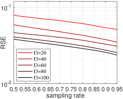
Considering the first data set, we investigate the effect of different tensor size on the performance of the proposed method. The sampling rate is varied from 0.05 to 0.5, with a step size equaling 0.05. Results are shown in Fig.3(a). Note that there exists a negative correlation between the tensor size and RSE. In particular, the underlying tensor can be recovered accurately with a much small sampling rate, when its size is large enough. In addition, for a fixed-size tensor, the RSE decreases monotonously with an increasing sampling rate. It is reasonable – the larger the number of observations is, the more information of the underlying tensor is obtained.
Furthermore, we study the influence of different on the recovery performance using the second data set. The sampling rate is varied from 0.05 to 0.5, with a step size equaling 0.05. Results are shown in Fig.3(b). At the same sampling rate, it can be seen that a larger leads to a smaller RSE. This conclusion is similar to the discussion of small and large in [38]. Moreover, with an increasing sampling rate, RSEs decreases monotonously.
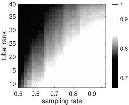
Considering the third data set, we investigate the effect of tubal rank on the recovery performance of the proposed method. The sampling rate is varied from 0.05 to 0.5, with a step size equaling 0.015. Furthermore, the PSNRs are normalized. Results are shown in Fig.4, where white means the underlying tensor is recovered successfully while black indicates that the recovery failed. As can be seen, the recovery performance can be guaranteed as long as the tubal rank is relatively low and the sampling rate is relatively large.
5.4 Color image data
Data sets: Zhou et al. [30] point out that most natural images have low tubal rank structure, and following the experiment settings in [39] and [40], we use four color images 11 1 https://github.com/Spring-Liu/testimage. to demonstrate the performance of the proposed method in this part. The four images (named lena, facade, baboon, and house, respectively) are resized to tensor. A summary of these four images is reported in Fig..
Baseline: We compare the performance of the proposed algorithm with other state-of-the-art methods, including: i) smooth PARAFAC tensor completion (SPC) [40] which is CP-rank based method, ii) the tensor n-rank based methods, i.e., simultaneous tensor decomposition and completion (STDC) [25], iii) the TT rank based methods, i.e., Tmac-TT [26] and tensor train stochastic gradient descent (TT-SGD) [34], and iv) TNN [33] which is the tubal rank based method.
| sr | method | lena | facade | baboon | house | ||||||||
|---|---|---|---|---|---|---|---|---|---|---|---|---|---|
| PSNR | RSE | SSIM | PSNR | RSE | SSIM | PSNR | RSE | SSIM | PSNR | RSE | SSIM | ||
| 0.1 | SPC | 25.5846 | 0.0948 | 0.7742 | 26.4615 | 0.0921 | 0.8189 | 21.0733 | 0.1638 | 0.5082 | 25.8000 | 0.0842 | 0.7979 |
| STDC | 19.7222 | 0.1862 | 0.4401 | 20.0552 | 0.1925 | 0.6117 | 16.9850 | 0.2622 | 0.3892 | 19.7105 | 0.1697 | 0.4099 | |
| Tmac-TT | 23.2412 | 0.1242 | 0.6972 | 19.7929 | 0.1985 | 0.6098 | 18.8118 | 0.2096 | 0.4046 | 23.1784 | 0.1145 | 0.6474 | |
| TT-SGD | 15.3518 | 0.2282 | 0.4245 | 20.8763 | 0.1731 | 0.6134 | 16.0909 | 0.2946 | 0.3520 | 16.8428 | 0.2448 | 0.3781 | |
| TNN | 24.1932 | 0.1080 | 0.7105 | 22.1981 | 0.1505 | 0.6571 | 20.6019 | 0.1729 | 0.4156 | 22.3312 | 0.1255 | 0.6060 | |
| proposed | 25.9028 | 0.0916 | 0.8015 | 24.3383 | 0.1180 | 0.7328 | 21.3046 | 0.1595 | 0.5145 | 25.9565 | 0.0828 | 0.8152 | |
| 0.2 | SPC | 27.4107 | 0.0768 | 0.8474 | 26.7079 | 0.0891 | 0.8740 | 22.2023 | 0.1438 | 0.6126 | 27.5046 | 0.0692 | 0.8480 |
| STDC | 25.8928 | 0.0915 | 0.8066 | 24.4484 | 0.1161 | 0.7727 | 19.6754 | 0.1924 | 0.4094 | 28.1505 | 0.0642 | 0.8673 | |
| Tmac-TT | 25.8833 | 0.0916 | 0.8015 | 22.0045 | 0.1538 | 0.6506 | 21.5952 | 0.1542 | 0.5884 | 25.9585 | 0.0826 | 0.8230 | |
| TT-SGD | 20.8364 | 0.1677 | 0.6224 | 25.2864 | 0.1067 | 0.7953 | 18.7745 | 0.2125 | 0.3959 | 21.4953 | 0.1363 | 0.4762 | |
| TNN | 26.0373 | 0.0900 | 0.8151 | 26.4776 | 0.0919 | 0.8213 | 21.9099 | 0.1487 | 0.6032 | 25.5434 | 0.0867 | 0.7918 | |
| proposed | 28.4658 | 0.0681 | 0.8820 | 27.9356 | 0.0783 | 0.8790 | 22.7415 | 0.1352 | 0.6565 | 29.3077 | 0.0566 | 0.8894 | |
| 0.3 | SPC | 28.7736 | 0.0657 | 0.8871 | 28.6894 | 0.0713 | 0.8927 | 23.2435 | 0.1276 | 0.7150 | 29.0217 | 0.0581 | 0.8828 |
| STDC | 27.9464 | 0.0722 | 0.8553 | 25.6342 | 0.1013 | 0.8092 | 21.7230 | 0.1520 | 0.5933 | 30.4959 | 0.0490 | 0.9129 | |
| Tmac-TT | 26.8824 | 0.0816 | 0.8341 | 23.6913 | 0.1267 | 0.7285 | 22.8057 | 0.1342 | 0.6657 | 26.9618 | 0.0736 | 0.8375 | |
| TT-SGD | 24.0597 | 0.1113 | 0.7066 | 28.1859 | 0.0750 | 0.8900 | 20.7091 | 0.1709 | 0.4982 | 24.1978 | 0.1010 | 0.6512 | |
| TNN | 28.0295 | 0.0715 | 0.8649 | 28.8579 | 0.0699 | 0.9100 | 22.9498 | 0.1320 | 0.6867 | 27.8168 | 0.0667 | 0.8652 | |
| proposed | 30.4150 | 0.0545 | 0.9324 | 30.1530 | 0.0602 | 0.9270 | 24.0340 | 0.1165 | 0.7626 | 32.1177 | 0.0407 | 0.9225 | |
| 0.4 | SPC | 30.0387 | 0.0568 | 0.9147 | 29.0100 | 0.0687 | 0.9142 | 24.2049 | 0.1142 | 0.7897 | 29.8044 | 0.0531 | 0.9070 |
| STDC | 29.1445 | 0.0629 | 0.8960 | 26.6845 | 0.0898 | 0.8721 | 23.4226 | 0.1250 | 0.7475 | 31.5988 | 0.0432 | 0.9180 | |
| Tmac-TT | 27.8189 | 0.0733 | 0.8511 | 25.5229 | 0.1026 | 0.8081 | 23.7994 | 0.1197 | 0.7497 | 27.9107 | 0.0660 | 0.8663 | |
| TT-SGD | 26.6475 | 0.0856 | 0.8272 | 29.6810 | 0.0619 | 0.9248 | 22.3022 | 0.1412 | 0.6204 | 25.8701 | 0.0831 | 0.8015 | |
| TNN | 29.8159 | 0.0582 | 0.9005 | 30.4659 | 0.0581 | 0.9337 | 23.9500 | 0.1176 | 0.7580 | 29.4037 | 0.0556 | 0.8934 | |
| proposed | 32.5232 | 0.0427 | 0.9582 | 31.3102 | 0.0527 | 0.9466 | 25.3032 | 0.1006 | 0.8308 | 33.6028 | 0.0343 | 0.9417 | |
For each color image, we test the above mentioned LRTC methods with sampling rate equaling 0.1, 0.2, 0.3 and 0.4. Results are shown in Table 1. As can be seen from Table 1, the performance improvement is universal for an increasing sampling rate. In particular, our proposed method is generally superior to other state-of-the-arts. More precisely, in addition to the results of facade at sampling rate 0.1, our method achieves highest PSNR, SSIM and smallest RSE. For further visually compare the recovery performance of all methods, we show the recovered results for each color image in Fig.5 (the sampling rate is fixed at 0.2). Note that the recovered color images of our method are closer to the original images. The reason of our method can obtain better details of images than TNN is that the proposed -TNN is a much tighter approximation of the tubal rank than tensor nuclear norm.
5.5 Hyperspectral image data
Data sets: In this part, we use two public hyperspectral image data sets named Washington DC Mall (WDC Mall) and Pavia University (paviaU)22
2
http://www.ehu.eus/ccwintco/index.php?title=Hyperspectral_Remote_Sensing_Scenes.. The whole WDC Mall data set contains pixels and 191 spectral bands, which is from the hyperspectral digital imagery collection experiment. In the following experiments, it is resized to a tensor. The whole paviaU data set is a pixels and 103 spectral bands image, which is from Pavia University. In the rest experiments, it is resized to a tensor. A visually summary is shown in Fig. 6.
Baseline: We compare the performance of the proposed algorithm with the same methods mentioned in color image experiments, i.e., SPC, STDC, Tmac-TT, TT-SGD, and TNN.
| sr | method | WDC Mall | PaviaU | ||
|---|---|---|---|---|---|
| PSNR | RSE | PSNR | RSE | ||
| 0.1 | SPC | 22.9355 | 0.1926 | 26.1087 | 0.2270 |
| STDC | 16.1068 | 0.4221 | 21.4573 | 0.3877 | |
| Tmac-TT | 16.5548 | 0.4009 | 21.6522 | 0.3791 | |
| TT-SGD | 17.4878 | 0.3606 | 21.0885 | 0.4045 | |
| TNN | 19.6377 | 0.2813 | 23.2825 | 0.3142 | |
| proposed | 22.9442 | 0.1924 | 27.3111 | 0.1976 | |
| 0.2 | SPC | 26.8823 | 0.1222 | 31.2002 | 0.1263 |
| STDC | 20.8547 | 0.2447 | 24.2979 | 0.2796 | |
| Tmac-TT | 18.7733 | 0.3105 | 23.4255 | 0.3091 | |
| TT-SGD | 20.0943 | 0.2668 | 24.7403 | 0.2657 | |
| TNN | 21.1869 | 0.2353 | 24.9034 | 0.2608 | |
| proposed | 27.6564 | 0.1118 | 31.4136 | 0.1234 | |
| 0.3 | SPC | 29.8279 | 0.0871 | 34.2700 | 0.0887 |
| STDC | 22.8627 | 0.1941 | 26.4978 | 0.2171 | |
| Tmac-TT | 20.5384 | 0.2534 | 25.0036 | 0.2577 | |
| TT-SGD | 21.7456 | 0.2206 | 26.2153 | 0.2242 | |
| TNN | 24.5025 | 0.1608 | 27.7402 | 0.1881 | |
| proposed | 30.0019 | 0.0854 | 34.4901 | 0.0865 | |
| 0.4 | SPC | 31.1864 | 0.0745 | 35.6849 | 0.0754 |
| STDC | 24.2289 | 0.1658 | 28.0926 | 0.1807 | |
| Tmac-TT | 22.0513 | 0.2129 | 26.6126 | 0.2142 | |
| TT-SGD | 23.2092 | 0.1863 | 27.5421 | 0.1924 | |
| TNN | 26.6422 | 0.1257 | 29.6721 | 0.1507 | |
| proposed | 32.1133 | 0.0669 | 36.9243 | 0.0653 | |
For the two hyperspectral images, we test the above mentioned LRTC methods with sampling rate equaling 0.1, 0.2, 0.3 and 0.4. Results are shown in Table 2. We use only PSNR and RSE as the evaluation metrics here. Similarly, we can see that our method almost outperforms others. The improvement of average recovery performance is statistically significant. To further prove the superiority of our proposed method for hyperspectral image inpainting, we show the recovered results of all methods from 0.2 sampling observed images in Fig.6, where only three slices of two data sets (the first three slices of WDC Mall and slices [60,61,62] of paviaU) are shown exemplarily. As can be seen from Fig.6, compared with other methods, our proposed algorithm visually performs better recovery results.
5.6 Conclusion
In this paper, we address the problem of low-rank tensor completion. We propose a new definition of tensor -shrinkage nuclear norm (-TNN). The tightness property of -TNN demonstrates that the proposed -TNN is a tighter surrogate of tensor average rank than tensor nuclear norm (TNN). Therefore, we propose a novel LRTC model by employing our proposed -TNN. In particular, the upper bound of recovery error for our LRTC model is further provided to show the underlying tensor can be recovered accurately. Accordingly, we develop an efficient algorithm by incorporating the adaptive momentum scheme. Subsequently, some theoretical analysis are provided from the aspects of complexity and convergence, respectively. The experimental results validate the superiority of our method over the state-of-the-arts.
However, there still several directions in future work. First, the experimental results show that further improvements are needed for the performance of our method at low sampling rate. Moreover, we will focus on the distributed version to apply it to massive data sets.
References
- [1] J. Liu, P. Musialski, P. Wonka, J. Ye, Tensor completion for estimating missing values in visual data, IEEE Trans. Pattern Anal. Mach. Intell. 35 (1) (2013) 208–220.
- [2] M. E. Kilmer, K. Braman, N. Hao, and R. C. Hoover, Third-order tensors as operators on matrices: A theoretical and computational framework with applications in imaging, SIAM Journal on Matrix Analysis and Applications, vol. 34, no. 1, pp. 148–172, 2013
- [3] Y. Wang, J. Peng, Q. Zhao, Y. Leung, X.L. Zhao, D. Meng, Hyperspectral image restoration via total variation regularized low-rank tensor decomposition, IEEE J. Sel. Top. Appl. Earth Obs. Remote Sens. 11 (4) (2018) 1227–1243.
- [4] Zhen Long, Yipeng Liu, Longxi Chen, Ce Zhu, low-rank Tensor Completion for Multiway Visual Data, Signal Processing (2018), doi: https://doi.org/10.1016/j.sigpro.2018.09.039
- [5] Z. Lai , Y. Xu , Q. Chen , J. Yang , D. Zhang , Multilinear sparse principal component analysis, IEEE Trans. Neural Netw. 25 (10) (2014) 1942–1950 .
- [6] Lu, C., Feng, J., Chen, Y., Liu, W., Lin, Z., Yan, S.. Tensor Robust Principal Component Analysis with A New Tensor Nuclear Norm, arXiv: 1804.03728 (2018).
- [7] A. Cichocki , D. Mandic , L. De Lathauwer , G. Zhou , Q. Zhao , C. Caiafa , H.A. Phan , Tensor decompositions for signal processing applications: from two-way to multiway component analysis, IEEE Signal Process. Mag. 32 (2) (2015) 145–163 .
- [8] F. Cong, Q.-H. Lin, L.-D. Kuang, X.-F. Gong, P. Astikainen, T. Ristaniemi, Tensor decomposition of EEG signals: a brief review, Journal of Neuroscience Methods 248 (2015) 59–69.
- [9] Z. Lai , Y. Xu , J. Yang , J. Tang , D. Zhang , Sparse tensor discriminant analysis, IEEE Trans. Image Process. 22 (10) (2013) 3904–3915 .
- [10] E.J. Candes̀ , T. Tao , The power of convex relaxation: near-optimal matrix completion, IEEE Trans. Inf. Theory 56 (5) (2010) 2053–2080 .
- [11] T. G. Kolda and B. W. Bader, Tensor decompositions and applications, SIAM review, vol. 51, no. 3, pp. 455–500, 2009.
- [12] J. B. Kruskal, Rank, decomposition, and uniqueness for 3-way and n-way arrays. North-Holland Publishing Co., 1989
- [13] L. R. Tucker, Some mathematical notes on three-mode factor analysis, Psychometrika, vol. 31, no. 3, pp. 279–311, 1966.
- [14] F. L. Hitchcock, The expression of a tensor or a polyadic as a sum of products, Studies in Applied Mathematics, vol. 6, no. 1-4, pp. 164–189, 1927.
- [15] H. A. Kiers, Towards a standardized notation and terminology in multiway analysis, Journal of Chemometrics, vol. 14, no. 3, pp. 105–122,2000.
- [16] I. V. Oseledets, Tensor-train decomposition, SIAM J. Sci. Comput., vol. 33, no. 5, pp. 2295–2317, Jan. 2011.
- [17] M. E. Kilmer and C. D. Martin, Factorization strategies for third-order tensors, Linear Algebra and its Applications, vol. 435, no. 3, pp. 641– 658, 2011.
- [18] S. Friedland and L.-H. Lim, Nuclear norm of higher-order tensors, Mathematics of Computation, vol. 87, no. 311, pp. 1255–1281, 2018.
- [19] Yuning Yang, Yunlong Feng, and Johan A. K. Suykens A Rank-One Tensor Updating Algorithm for Tensor Completion. IEEE SIGNAL PROCESSING LETTERS, VOL. 22, NO. 10, OCTOBER 2015 1633
- [20] M. Yuan and C.-H. Zhang, On tensor completion via nuclear norm minimization, Foundations ofComputational Mathematics, 16(4) (2016) 1031–1068.
- [21] C. J. Hillar and L.-H. Lim, Most tensor problems are NP-hard, J. ACM,vol. 60, no. 6, 2013, Art. no. 45.
- [22] S. Gandy, B. Recht, I. Yamada, Tensor completion and low-n-rank tensor recovery via convex optimization, Inverse Problems 27 (2) (2011) 1–19.
- [23] Marco Signoretto, Quoc Tran Dinh, Lieven De Lathauwer, and Johan A. K. Suykens. 2014. Learning with tensors: A framework based on convex optimization and spectral regularization. Machine Learning 94, 3 (2014), 303–351.
- [24] H. Kasai and B. Mishra, Low-rank tensor completion: a Riemannian manifold preconditioning approach, in International Conference on Machine Learning, pp. 1012–1021, 2016.
- [25] Y.-L. Chen, C.-T. Hsu, and H.-Y. M. Liao, Simultaneous tensor decomposition and completion using factor priors, IEEE Transactions on Pattern Analysis and Machine Intelligence, vol. 36, no. 3, pp. 577–591, 2014.
- [26] Bengua, J. A., Phien, H. N., Tuan, H. D., Do, M. N. (2017). Efficient Tensor Completion for Color Image and Video Recovery: Low-Rank Tensor Train. IEEE Transactions on Image Processing, 26(5), 2466–2479.
- [27] Imaizumi, M., Maehara, T., Hayashi, K. (2017). On Tensor Train Rank Minimization: Statistical Efficiency and Scalable Algorithm. (Nips 2017).
- [28] Z. Zhang, G. Ely, S. Aeron, N. Hao, and M. Kilmer, Novel methods for multilinear data completion and de-noising based on tensor-SVD, in Proceedings of the IEEE Conference on Computer Vision and Pattern Recognition, pp. 3842–3849, 2014.
- [29] Z. Zhang, and S. Aeron. Exact tensor completion using t-SVD. IEEE Transactions on Signal Processing, 65(6): 1511-1526, 2017.
- [30] P. Zhou, C. Lu, Z. Lin, and C. Zhang, Tensor factorization for low-rank tensor completion, IEEE Transactions on Image Processing, vol. 27, no. 3, pp. 1152–1163, 2018.
- [31] Kong, H., Xie, X., Lin, Z. (2018). t-Schatten- Norm for Low-Rank Tensor Recovery. IEEE Journal of Selected Topics in Signal Processing, 12(6), 1405–1419. https://doi.org/10.1109/jstsp.2018.2879185
- [32] S. Voronin and R. Chartrand. A new generalized thresholding algorithm for inverse problems with sparsity constraints. In IEEE International Conference on Acoustics, Speech and Signal Processing (ICASSP), 1636-1640, 2013.
- [33] C. Lu, J. Feng, Y. Chen, W. Liu, Z. Lin, and S. Yan, Tensor robust principal component analysis: Exact recovery of corrupted low-rank tensors via convex optimization, in Proceedings of the IEEE Conference on Computer Vision and Pattern Recognition, pp. 5249–5257, 2016.
- [34] Wang, A., Lai, Z., Jin, Z. (2019). Noisy low-tubal-rank tensor completion. Neurocomputing, 330, 267–279. https://doi.org/10.1016/j.neucom.2018.11.012
- [35] Duchi, J., Hazan, E., and Singer, Y. Adaptive subgradient methods for online learning and stochastic optimization. JMLR, 12(Jul):2121–2159, 2011.
- [36] Li, Q., Zhou, Y., Liang, Y., and Varshney, P. Convergence analysis of proximal gradient with momentum for nonconvex optimization. In ICML, pp. 2111–2119, 2017.
- [37] Q. Yao, J. Kwok, B. Han. Efficient Nonconvex Regularized Tensor Completion with Structure-aware Proximal Iterations. International Conference on Machine Learning (ICML). 2019.
- [38] yao, quanming, Kwok, J. T., Wang, T. F., Liu, T. Y. (2018). Large-Scale Low-Rank Matrix Learning with Nonconvex Regularizers. IEEE Transactions on Pattern Analysis and Machine Intelligence, 8828(c), 1–16. https://doi.org/10.1109/TPAMI.2018.2858249
- [39] Biao Xiong ; Qiegen Liu ; Jiaojiao Xiong ; Sanqian Li ; Shanshan Wang ; Dong Liang. Field-of-Experts Filters Guided Tensor Completion. IEEE Transactions on Multimedia. 20(9) (2018), 2316-2329.
- [40] Tatsuya Yokota ; Qibin Zhao ; Andrzej Cichocki. Smooth PARAFAC Decomposition for Tensor Completion, IEEE Transactions on Signal Processing, 64(20) (2016), 5423-5436.
- [41] O. Klopp et al., Noisy low-rank matrix completion with general sampling distribution, Bernoulli, vol. 20, no. 1, pp. 282–303, 2014.