The Integrated Nested Laplace Approximation for fitting Dirichlet regression models

The Dirichlet distribution is the generalization of the widely known Beta distribution, and it is defined by the following probability density,

where ${\bm{\alpha}}=(\alpha_{1},\ldots,\alpha_{C})$ is known as the vector of shape parameters for each category, $\alpha_{c}>0$ $\forall c$, $y_{c}\in(0,1)$, $\sum_{c=1}^{C}y_{c}=1$, and $\text{B}({\bm{\alpha}})$ is the Multinomial Beta function, which serves as the normalizing constant. The Multinomial Beta function is defined as $\prod_{c=1}^{C}\Gamma(\alpha_{c})/\Gamma(\sum_{c=1}^{C}\alpha_{c})$. The sum of all $\alpha$’s, $\alpha_{0}=\sum_{c=1}^{C}\alpha_{c}$, is usually interpreted as a precision parameter ($\tau$). The Beta distribution is the particular case when $C=2$. In addition, each variable is marginally Beta distributed with $\alpha=\alpha_{c}$ and $\beta=\alpha_{0}-\alpha_{c}$.

Let ${\bm{y}}\sim\mathcal{D}({\bm{\alpha}})$ denote a variable that is Dirichlet distributed. The expected values are $\text{E}(y_{c})=\alpha_{c}/\alpha_{0}$, the variances are $\text{Var}(y_{c})=[\alpha_{c}(\alpha_{0}-\alpha_{c})]/[\alpha_{0}^{2}(\alpha_{0}+1)]$ and the covariances are $\text{Cov}(y_{c},y_{c^{\prime}})=(-\alpha_{c}\alpha_{c^{\prime}})/[\alpha_{0}^{2}(\alpha_{0}+1)]$.

Let ${\bm{Y}}$ be a matrix with $C$ rows and $N$ columns denoting $N$ observations for the different categories $C$ of the $C$ dimensional response variable ${\bm{Y}}_{\bullet n}\sim\mathcal{D}({\bm{\alpha}}_{n})$. Let $\eta^{*}_{cn}$ be the linear predictor for the $n$th observation in the $c$th category, so ${\bm{\eta}}^{*}$ is a matrix with $C$ rows and $N$ columns. Let ${\bm{V}}^{(c)}$, $c=1,\ldots,C$, represents a matrix with dimension $N\times J_{c}$ that contains the covariate values for each individual and each category, so ${\bm{V}}^{(c)}_{n\bullet}$ shows the covariate values for the $n$th observation and the $c$th category. Let ${\bm{\beta}}$ be a matrix with $J_{c}$ rows and $C$ columns representing the regression coefficients in each dimension. Finally, let also $\omega_{cn}$ represents a realization of a random effect for the the $c$th category and the $n$th observation. Then, the relationship between the parameters of the Dirichlet distribution and the elements of the linear predictor (including random effects) is set up as:

where $g(\cdot)$ is the link-function. As $\alpha_{c}>0$ for $c=1,\ldots,C$, log-link $g(\cdot)=\log(\cdot)$ is used. The regression coefficients ${\bm{\beta}}_{\bullet c}$ are a column vector with $J_{c}$ elements.

Dirichlet distributions can also be parametrized in terms of the mean $\mu_{cn}=\frac{\alpha_{cn}}{\sum_{n=1}^{N}\alpha_{cn}}$ and the precision $\tau$. In this case, the relationship between the mean and the linear predictor is stated as:

The regression coefficients ${\bm{\gamma}}_{\bullet c}$ are now a column vector with $J_{c}$ elements, while $\omega_{cn}^{{\bm{\mu}}}$ represents now a realization of a random effect in this parametrization. Moreover, as one of the categories can be obtained as one less the sum of the rest, we can employ the same Multinomial logit strategy used in Multinomial regression: linear predictor of one category (base category) is set to zero, whereby this category is virtually omitted and becomes the reference.

The equivalence between the two parametrizations comes from the equalities

and

where $\tilde{{\bm{\gamma}}}_{\bullet c}$ is a column vector with $J\geq J_{c}$ elements that contains $J_{c}$ non-zero elements and $J-J_{c}$ zero-elements. $J$ dimension comes from a general matrix $\bm{V}$ with dimension $N\times J$ which contains all the covariates values ($J$) for all the observations used in all the categories. $\tilde{{\bm{\beta}}}_{\bullet c}$ is also a column vector with $J\geq J_{c}$ elements, and $\tilde{{\bm{\beta}}}_{\bullet r}$ and $\omega_{rn}$ are the regression coefficients and the realization of a random effect for the base category respectively.

Note that we can include in the formula as many random effects as we consider and from a different nature: temporal, spatial, etc. But here, without loss of generality, we have added just one to show the equivalence between both parametrizations (proof in Appendix A). As the proposal presented in the following Sections relies on the fact that there are no other parameters to estimate in the observation likelihood, from now on we focus on the first parametrization presented.

Equation (3) can be rewritten in a vectorized form. In particular, if

denotes a restructured linear predictor, being ${\bm{\eta}}^{*}_{\bullet n}$ a column vector representing the linear predictor for the $n$th observation and all the categories, the model in matrix notation is

where ${\bm{A}}$ is the matrix properly constructed with the covariates values and vectors of 1s for the random effects, and ${\bm{x}}$ a vector formed by the regression coefficients plus the realizations of the random effects. Posteriorly, we will refer to this vector as the Latent Gaussian random field.

The popularity of INLA stems from the fact that it allows for fast approximate inference for LGMs, which are a large class of models that include a lot of classically important models (Rue and Held 2005). LGMs can be written as a three-stage hierarchical model in which observations ${\bm{y}}$ can be assumed to be conditionally independent given a latent Gaussian random field ${\bm{x}}$ and hyperparameters ${\bm{\theta}}_{1}$, y ∣x, θ_1 ∼∏_n=1^N p(y_n ∣x_n, θ_1) . The versatility of the model class relates to the specification of the latent Gaussian field x ∣θ_2 ∼N(μ(θ_2), Q^-1(θ_2)) which includes all the latent (non-observable) components of interest, such as fixed effects and random terms, describing the underlying process of the data. The hyperparameters ${\bm{\theta}}=({\bm{\theta}}_{1},{\bm{\theta}}_{2})$ control the latent Gaussian field and/or the likelihood for the data.

The LGMs are a class generalising the large number of related variants of additive and generalized models. If the likelihood $p(y_{n}\mid x_{n},{\bm{\theta}})$ such that “$y_{n}$ only depends on its linear predictor $\eta_{n}$” yields the generalized linear model setup, the set $\{x_{n},n=1,\ldots,N\}$ can be interpreted as $\eta_{n}$, being $\eta_{n}$ the linear predictor which is additive with respect to other effects,

where $\beta_{0}$ is the intercept, ${\bm{v}}$ represents the fixed covariates with linear effects $\{\beta_{j}\}$, and the terms $\{{\bm{\omega}}_{k}\}$ represent specific Gaussian processes. Each $\omega_{kn}$ is the contribution of the model components ${\bm{\omega}}_{k}$ to the $n$th linear predictor (Rue et al. 2017). If a Gaussian prior is assumed for the intercept and the parameters of the fixed effects, the joint distribution of ${\bm{x}}=\{{\bm{\eta}},\beta_{0},{\bm{\beta}},{\bm{\omega}}_{1},{\bm{\omega}}_{2},\ldots\}$ is a priori Gaussian. This yields the latent field ${\bm{x}}$ in the hierarchical LGM formulation. The hyperparameters ${\bm{\theta}}$ contain the non-Gaussian parameters of the likelihood and the model components. These parameters commonly include variance, scale, or correlation parameters.

In many important cases, the latent field is not only Gaussian, but also sparse Gaussian Markov random field (Rue and Held 2005, GMRF). A GMRF is a multivariate Gaussian random variable with additional conditional independence properties: $x_{j}$ and $x_{j}^{\prime}$ are conditionally independent given the remaining elements if and only if the $(i,j)$ entry of the precision matrix is $0$. Implementations of the INLA method frequently use this property to speed up computation.

Laplace approximation (Barndorff-Nielsen and Cox 1989) is a technique used to approximate integrals of the form

The main idea is to approximate the target with a scaled Gaussian density that matches the value and the curvature of the target distribution at the mode and evaluate the integral using this Gaussian instead. If $x_{0}$ is the point where $f(x)$ has its maximum, then

If $nf(x)$ is interpreted as the sum of log-likelihoods and $x$ as the unknown parameter, the Gaussian approximation will be very accurate as $n\rightarrow\infty$ under appropriate regularity conditions.

If we are interested in computing a marginal distribution $p(\gamma_{1})$ from a joint distribution $p({\bm{\gamma}})$, the Laplace approximation of the integral $\int p({\bm{\gamma}})\,\mathrm{d}{\bm{\gamma}}_{-1}$ can be expressed as follows:

where the first equality holds for any valid ${\bm{\gamma}}^{*}_{-1}$, and the mean ${\bm{\mu}}(\gamma_{1})$ and precision ${\bm{Q}}(\gamma_{1})$ are the parameters of the multivariate Gaussian density derived from the derivatives of $\log p({\bm{\gamma}})$ with respect to ${\bm{\gamma}}_{-1}$, for fixed $\gamma_{1}$. If the posterior is close to a Gaussian density, the results will be more accurate than if the posterior is very non-Gaussian. In this context, unimodality is necessary since the integrand is being approximated with a Gaussian at the mode ${\bm{\gamma}}^{*}_{-1}={\bm{\mu}}(\gamma_{1})$.

The main idea of INLA approach is to approximate the posteriors of interest: the marginal posteriors for the latent field, $p(x_{m}\mid{\bm{y}})$, and the marginal posteriors for the hyperparameters, $p(\theta_{k}\mid{\bm{y}})$. These posteriors can be written as

The nested formulation is used to compute $p(x_{m}\mid{\bm{y}})$ by approximating $p(x_{m}\mid{\bm{\theta}},{\bm{y}})$ and $p({\bm{\theta}}\mid{\bm{y}})$, and then using numerical integration to integrate out ${\bm{\theta}}$. Similarly, $p(\theta_{k}\mid{\bm{y}})$ can be computed by approximating $p({\bm{\theta}}\mid{\bm{y}})$ and integrating out ${\bm{\theta}}_{-k}$.

The marginal posterior distributions in (12) and (13) are computed using the Laplace approximation presented in subsection 3.2. In Rue et al. 2009 it is shown that the nested approach yields a very accurate approximation if applied to LGMs.

All this methodology can be used through R with the R-INLA package. For more details about R-INLA we refer the reader to Blangiardo and Cameletti 2015; Zuur et al. 2017; Wang et al. 2018; Krainski et al. 2018; Moraga 2019; Gómez-Rubio 2020, where practical examples and code guidelines are provided.

However, and despite the advantages of R-INLA implementation, there are some limitations when we deal with multivariate responses. The Multinomial case is solved, as the Multinomial likelihood can be approximated using the Poisson trick. It consists of transforming the Multinomial likelihood into a Poisson likelihood with additional parameters (Baker 1994). However, there is no method available when we deal with compositional data. In what follows, we propose an expansion of the INLA method for a Dirichlet response variable.

Let ${\bm{\eta}}_{n}:={\bm{\eta}}^{*}_{\bullet n}$ denote the linear predictor corresponding to the $n$th observation ${\bm{y}}_{n}:={\bm{Y}}_{\bullet n}$. If $l({\bm{y}}\mid{\bm{x}})$ represents $-\log p({\bm{y}}\mid{\bm{x}})$ for any ${\bm{y}}$ and ${\bm{x}}$, then $l({\bm{y}}_{n}\mid{\bm{\eta}}_{n})=-\log p({\bm{y}}_{n}\mid{\bm{\eta}}_{n})$ is the log-likelihood function expressed for the $n$th observation, being ${\bm{y}}_{n}$ and ${\bm{\eta}}_{n}$ vectors with $C$ components. Moreover, if ${\bm{\eta}}^{0}_{n}$ is a vector with dimension $C$, we express the gradient of $l({\bm{y}}_{n}\mid{\bm{\eta}}_{n})$ in ${\bm{\eta}}^{0}_{n}$ as ${{\bm{g}}^{0}_{\bm{\eta}}}_{n}=\nabla_{{\bm{\eta}}_{n}}(l)({\bm{\eta}}^{0}_{n},{\bm{y}}_{n})$, and the Hessian of $l({\bm{y}}_{n}\mid{\bm{\eta}}_{n})$ in ${\bm{\eta}}^{0}_{n}$ as ${\bm{H}}^{0}_{{\bm{\eta}}_{n}}$. Depending on which is more computationally convenient, ${\bm{H}}^{0}_{{\bm{\eta}}_{n}}$ can be either the true Hessian ($\nabla^{2}_{{\bm{\eta}}_{n}}(l)({\bm{\eta}}^{0}_{n},{\bm{y}}_{n})$) or the expected Hessian ($\text{E}_{{\bm{y}}_{n}\mid{{\bm{\eta}}_{n}}}(\nabla^{2}_{{\bm{\eta}}_{n}}(l)({\bm{\eta}}^{0}_{n},{\bm{y}}_{n}))$) in ${\bm{\eta}}^{0}_{n}$. Let ${\bm{L}}^{0}_{n}$ be the result of applying the Cholesky factorization to ${\bm{H}}^{0}_{{\bm{\eta}}_{n}}$, ${\bm{H}}^{0}_{{\bm{\eta}}_{n}}={\bm{L}}^{0}_{n}({\bm{L}}^{0}_{n})^{T}$.

Theorem 4.1 allows us to convert the observation vector ${\bm{y}}_{n}$ into Gaussian conditionally independent pseudo-observations ${\bm{z}}^{0}_{n}$. More importantly, this theorem can be expanded to multiple observations. In particular, if we denote

then the following proposition stands.

This approximation has been constructed for a generic ${\bm{\tilde{\eta}}}^{0}$, but, as we are interested in building a Gaussian approximation of the effect of the likelihood on the posterior distribution, ${\bm{\tilde{\eta}}}^{0}$ has been chosen as the posterior mode of $l({\bm{\tilde{\eta}}}\mid{\bm{Y}})$. Then:

The model posterior is factorized as:

and the approximation is factorized as:

Note that the approximation is constructed for a generic ${\bm{\tilde{\eta}}}$, in other words, this approximation is conditionally dependent on the linear predictor. The linear predictor can be formed by fixed effects or random effects. Here, in the implementation of the algorithm, we focus on the case where fixed effects and iid random effects are added to the linear predictor.

In what follows, we depict the different steps to compute the marginal posterior distributions of the latent field, $p({\bm{x}}_{m}\mid{\bm{Y}})$, and the marginal posterior distribution of the hyperparameters $p({\bm{\theta}}_{k}\mid{\bm{Y}})$. To obtain them, it is necessary to numerically find the mode of the posterior distribution of the linear predictor ${\bm{\tilde{\eta}}}^{0}$. This can be done by means of an iterative method in a similar way to inlabru (Bachl et al. 2019). We define a functional $f(\overline{p}_{{\bm{u}}})$ of the posterior distribution at ${\bm{u}}$ which generates a latent field configuration. Our aim is to find an invariant point of the functional, so that ${\bm{x}}^{0}=f(\overline{p}_{{\bm{x}}^{0}})$. The choice for $f(\cdot)$ is the joint conditional mode $f(\overline{p}_{{\bm{x}}})=$ arg max${}_{{\bm{x}}}\overline{p}_{{\bm{x}}}({\bm{x}}\mid{\bm{\tilde{z}}}^{0},{\bm{\theta}}^{0})$, being ${\bm{\theta}}^{0}=$ arg max${}_{{\bm{\theta}}}\overline{p}_{{\bm{\theta}}}({\bm{\theta}}\mid{\bm{\tilde{z}}}^{0})$. The final algorithm is:

1. 1.

   Let ${\bm{x}}^{1}$ and ${\bm{\theta}}^{1}$ be initial candidate points for the latent variables and the hyperparameters.

2. 2.

   Locate a good candidate in the latent variables for the computation of the new pseudo-observations. Compute the mode (${\bm{x}}^{2}$) in ${\bm{x}}$ of $p({\bm{x}}\mid{\bm{Y}},{\bm{\theta}}^{1})$ by means of a quasi-Newton method (Dennis and Moré 1977) with line search strategy and Armijo conditions (Nocedal and Wright 2006) in $-\log(p({\bm{x}}\mid{\bm{Y}},{\bm{\theta}}^{1})\propto l({\bm{Y}}\mid{\bm{x}},{\bm{\theta}}^{1})+l({\bm{x}}\mid{\bm{\theta}}^{1})$, being $p({\bm{x}}\mid{\bm{\theta}}^{1})$ multivariate Gaussian as we are in the LGMs context. ${\bm{\tilde{\eta}}}^{1}$ can be easily calculated from the expression ${\bm{\tilde{\eta}}}={\bm{A}}{\bm{x}}$.

3. 3.

   Calculate the conditionally independent Gaussian pseudobservations ${\bm{\tilde{z}}}^{1}$. In this case, at the modal configuration established ${\bm{x}}^{1}$, the Hessian matrix ${\bm{H}}^{1}_{{\bm{\tilde{\eta}}}}$ is computed. If the submatrix corresponding to the $n$th individual ${\bm{H}}^{1}_{\tilde{{\bm{\eta}}}_{n}}$ is not positive definite, the expected Hessian is used instead to guarantee a positive definite ${\bm{H}}^{1}_{{\bm{\tilde{\eta}}}}$. Following the approximation previously presented, the Cholesky factorization is computed in ${\bm{H}}^{1}_{{\bm{\tilde{\eta}}}}={\bm{L}}^{1}({\bm{L}}^{1})^{T}$. The gradient (${\bm{g}}^{1}_{{\bm{\tilde{\eta}}}}$) is also calculated in ${\bm{\tilde{\eta}}}^{1}$. According to the equation (16), the scale and rotation of the original observations are done to get the pseudo-observations ${\bm{\tilde{z}}}^{1}$.

4. 4.

   Call R-INLA. As pseudo-observations ${\bm{\tilde{z}}}^{1}$ are conditionally independent Gaussian observations, we are able to call R-INLA. If in Step 2 algorithm has converged for a given tolerance, the posterior distributions obtained here are the one that we were looking for: $\overline{p}({\bm{\theta}}\mid{\bm{\tilde{z}}}^{1})$ and $\overline{p}({\bm{x}}\mid{\bm{\tilde{z}}}^{1})$. Else, repeat from step 1 defining ${\bm{x}}^{3}=f(\overline{p}_{{\bm{x}}^{2}})$ as the new starting point for the latent variables, and ${\bm{\theta}}^{2}=$ arg max${}_{{\bm{\theta}}}\overline{p}_{{\bm{\theta}}}({\bm{\theta}}\mid{\bm{\tilde{z}}}^{1})$ the new starting point for the hyperparameters.

After depicting the complete method, we focus on an implementation in R (R Core Team 2021) of this approximation.

This subsection presents an example of how simulation can be conducted using the functions of dirinla.

First, we simulate the covariates from a Uniform(0,1):

R> N <- 100R> V <- as.data.frame(matrix(runif((3) * N, 0, 1), ncol = 3))R> names(V) <- paste0(’v’, 1:3)

We then define the formula that we want to fit to keep the values of the different categories in a list. This object will be used to construct the ${\bm{A}}$ matrix. We use the function formula_list() from the package dirinla.

R> formula <- y ~ 1 + v1 | 1 + v2 | 1 + v3R> names_cat <- formula_list(formula)

The values for the parameters composing the latent field are assigned to conduct the simulation. As we have previously depicted, $\beta_{01}=-1.5$, $\beta_{02}=-2$, $\beta_{03}=0$ are the intercepts, and $\beta_{11}=1$, $\beta_{12}=2.3$, $\beta_{13}=-1.9$ are the slopes:

R> x <- c(-1.5, 1, -2, 2.3, 0, -1.9)We call the function data_stack_dirich() of the package dirinla to construct the ${\bm{A}}$ matrix presented in previous sections. This function uses the inla.stack() structure of the package R-INLA. As a consequence, the returning object is an inla.stack object. Observe that the arguments are the response variable y (in this case it has not been generated yet), the names of the categories covariates, a matrix with the values of the covariates data, the number of categories d and the number of observations N. The sparse matrix ${\bm{A}}$ is then computed.

R> mus <- exp(x) / sum(exp(x))R> C <- length(names_cat)R> A_construct <-+ data_stack_dirich(y = as.vector(rep(NA, N * C)),+ covariates = names_cat,+ data = V,+ d = C,+ n = N)The next step is to construct the linear predictor as ${\bm{\tilde{\eta}}}={\bm{A}}{\bm{x}}$ using the parameters fixed in the latent field. Using the exponential transformation it is easy to get the parameters ${\bm{\alpha}}$ of the Dirichlet distribution:

R> eta <- A_construct %*% xR> alpha <- exp(eta)

The last stage is to generate the response variable using the function rdirichlet() from DirichletReg (Maier 2014). The output is a matrix with the response variable summing their rows up to one.

R> y <- rdirichlet(N, alpha)

We now present the functions of dirinla needed to fit Dirichlet regression models, the main one being dirinlareg. This function carries out all the steps presented in Section 4, and its use (for the simulated data from previous subsection) is as follows:

R> model.inla <- dirinlareg(+ formula = y ~ 1 + v1 | 1 + v2 | 1 + v3 ,+ y = y,+ data.cov = V,+ prec = 0.0001,+ verbose = FALSE)where we have to specify the model formula, the response variable ${\bm{Y}}$ in a matrix format, the data.frame with the covariates data.cov, and the precision of the Gaussian prior (prec) for the latent field ${\bm{x}}$. If we want to follow the process step by step, we can add the instruction verbose = TRUE.

Once the model is fitted, we can summarize the posterior distribution of the fixed effects by means of the function summary applied to the object generated. This object belongs to the dirinlaregmodel class. Three model selection criteria are also displayed: Deviance Information Criterion (Spiegelhalter et al. 2002, DIC), Watanabe-Akaike information criteria (Gelman et al. 2014, WAIC), and the mean of the logarithm of the conditional predictive ordinate (Gneiting and Raftery 2007, LCPO). Lastly, the number of observations and the number of categories are also depicted (Table 1).

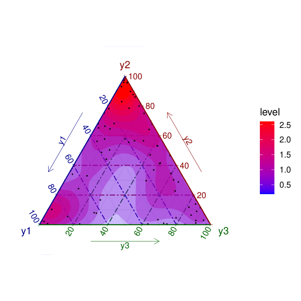
Using the implemented plot method, we obtain the marginal posterior distributions of the latent field for the different categories (Figure 1). These marginals and a summary of each one are stored in model.inla$marginals_fixed and model.inla$summary_fixed (see example.R from the supplementary code to see the details of the code). The plot method also depicts the posterior predictive distribution in the simplex (Figure 2).

Finally, the posterior distribution for the scale parameters of the Dirichlet $\alpha$ can also be computed. In particular, model.inla$marginals_fixed and model.inla$summary_fixed provide the marginals and a summary for each category. Mean parameters can also be obtained via model.inla$marginals_means or model.inla$summary_means, and similarly, model.inla$marginals_precision or model.inla$summary_precision provides the precision parameters.

In most cases, practitioners want to be able to predict the composition of a new observation. The package also provides a function predict to compute posterior predictive distributions for new individuals. To show how it works, we now present how to predict for a value of v1 = 0.2, v2 = 0.5, and v3 = -0.1:

R> model.prediction <-+ predict(model.inla,+ data.pred.cov = data.frame(v1 = 0.2 ,+ v2 = 0.5,+ v3 = -0.1))The resulting object also belongs to the dirinlaregmodel class. In a similar way as above, the elements summary_predictive_alphas and marginals_predictive_alphas describe the posterior predictive distribution for the scale parameters of the Dirichlet ${\bm{\alpha}}$, obtained for the new values of the covariates. In addition, means ($\mu$) and precisions ($\tau$) are available via summary_predictive_means, marginals_predictive_means, summary_predictive_precision and marginals_predictive_precision

Our first setting is based on a Dirichlet regression with four categories and one parameter per category, the intercept, that is:

Five different datasets of sizes $N=50,100$, $500,1000,10000$ with this structure were simulated letting $\beta_{0c},c=1,\ldots,4$ to be $-2.4$, $1.2$, $-3.1$ and $1.3$, respectively. We used vague prior distributions for the latent field ($\bm{x}=$ {$\beta_{0c},c=1,\ldots,4$}). In particular, $p(x_{m})\sim$ $\mathcal{N}(0,\tau=0.0001)$, $m=1,\ldots,4$. As the response values are not close to 0 and 1, no transformation was needed.

As above mentioned, for each simulated dataset, we employed three different methods to make inference: a standard application of the R-JAGS package with $2000$ iterations, a burnin of $200$, a thin number of $5$ and $3$ chains; the INLA methodology through the dirinla package; and long R-JAGS, using $1000000$ iterations with a burnin of $100000$, a thin number of $5$ and $3$ chains. To compare methodologies, the strategies presented at the begining of the section were used.

As seen in Figure 3 (the rest of the plots are shown in the Simulation 1 of the supplementary material in https://jmartinez-minaya.github.io/supplementary/CODA/tests.html), the posterior densities have similar shape, with the new method tending to agree more with the long R-JAGS result than the more variable short run R-JAGS does, illustrating how our method reduces estimator variability, at the potential cost of a generally small bias.

With respect the computational effort needed to get those results, Figure 4 displays that, dirinla methodology has a faster computational speed for given data sizes, for the given R-JAGS chain lengths.

In Figure 5, we see that $ratio_{1}$-dirinla is so closed to 0 as happen with $ratio_{1}$-R-JAGS, and $ratio_{2}$-dirinla is always close to 1, similar to $ratio_{2}$-R-JAGS, meaning that using dirinla we obtain as good approximations as with R-JAGS reducing considerably the computational cost.

The second setting is based on a Dirichlet regression with a different covariate per category:

Again, we simulated five different datasets of sizes $N=50,100$, $500,1000,10000$. We set values for $\beta_{0c}$ and $\beta_{1c}$, $c=1,\ldots,4$ to $-1.5,1,-3,1.5,2,-3,-1,5$ respectively, and we simulated covariates from a Uniform distribution with mean in the interval $(0,1)$. We assigned vague prior distributions for the latent field ($\bm{x}=${$\beta_{0c},\beta_{1c},c=1,\ldots,4$}). Particularly, $p(x_{m})\sim$ $\mathcal{N}(0,\tau=0.0001)$, $m=1,\ldots,8$. As the data generated did not present zeros and ones, we did not use any transformation.

As in the previous simulation, we employed the same three different inference methods with the same configurations and the four strategies used in the previous simulation. In Figure 6 (see Simulation 2 in https://jmartinez-minaya.github.io/supplementary/CODA/tests.html for further plots), the posterior distributions are similar in both $\beta_{0c}$ and $\beta_{1c}$, $c=1,\ldots,4$.

Figure 7 depicts that dirinla has a faster computational speed for given data sizes and for given R-JAGS chain lengths. In Figure 8, we show that $ratio_{1}$-dirinla and $ratio_{1}$-R-JAGS are so close to 0 in all cases, and $ratio_{2}$-dirinla and $ratio_{2}$-R-JAGS are always close to 1. Again, we conclude that using dirinla we get similar approximations to R-JAGS, while substantially reducing the computational cost.

The third setting is based on a Dirichlet regression with a different covariate per category without intercept and adding two shared independent random effects.

We simulated four different datasets of sizes $N=50,100$, $500,1000$. We set values for $\beta_{1c}$ for $c=1,\ldots,4$ to $-1.5,2,1,-3$ respectively, and we simulated covariates from a Uniform distribution on the interval $(-1,1)$. Random effects ${\bm{\omega}}_{1}$ and ${\bm{\omega}}_{2}$ were simulated from Gaussian distributions with mean 0 and standard deviations $\sigma_{1}=1/2$ (precision $\tau_{1}=4$) and $\sigma_{2}=1/3$ (precision $\tau_{2}=9$) varying the levels of the factor ($I$), in particular, they were set to $I=2,5,10,25$. The $i_{n}$ sub-index assigns each individual $n$ to a level of the factor.

As we are in the context of Bayesian LGMs, we established Gaussian prior distributions for the latent field, in this case, formed by the parameters corresponding to the fixed effects and the random effects. In particular, we assigned Gaussian prior distributions with mean 0 and precision $0.0001$ to {$\beta_{1c},c=1,\ldots,4$}, and Gaussian priors distribution with mean $0$ and precisions $\tau_{1}$ and $\tau_{2}$ for the two shared random effects ${\bm{\omega}}_{1}$ and ${\bm{\omega}}_{2}$. Two types of priors for the $\tau_{1}$ and $\tau_{2}$ parameters were employed. Half-Gaussian priors with location $0$ and precision parameter $1$ were used for R-JAGS, long R-JAGS and dirinla. For dirinla, and additional model with a PC-prior(1, 0.01) (Simpson et al. 2017) was also used. The generated data did not contain zeros and ones, so we did not use any transformation. As these models have two hyperparameters, we increased the number of iterations of the R-JAGS method to $20000$ and burnin to $2000$ to achieve a given effective sample size of the MCMC method.

In Figures 9 and 10 (see Simulation 3 in the supplementary material, https://jmartinez-minaya.github.io/supplementary/CODA/tests.html for the complete simulation summaries), we display the posterior distribution of the parameters and the hyperparameters with 2 levels in the factors obtained with the different methods and the different priors. In the case of the precision parameters, we also depict the priors used for them: PC-prior (pc) and Half Gaussian (hn). We observe that the shapes of the posterior densities are similar in all the cases.

Figure 11 shows that dirinla provides higher computational efficiency. And, in view of Figure 12, $ratio_{1}$-dirinla and $ratio_{1}$-R-JAGS are both closed to 0. Similar is the behaviour of $ratio_{2}$, in both cases, it is closed to 1, proving that when we include random effects in the model, we can also get similar approximations by decreasing the computational cost.

If we look at the rest of the simulations conducted (See Simulation 3 in the supplementary material, https://jmartinez-minaya.github.io/supplementary/CODA/tests.html), we observe that large $N$ and small $J$ shows the influence of the different priors. And large $J$ display the difficulties of dirinla in approaching the posterior of the hyperparameters.

This last simulation is based on a Dirichlet regression with just one parameter per category and without covariates as in Simulation 1. The idea is that for a fixed data size, we increase the number of categories and then simulate from all those models and compare inferential methods. In particular, we used $N=100$ and $C=5,10,15,20$ and $30$. We also employed R-JAGS, dirinla with the same configuration as in simulations 1 and 2. However, in the case of long R-JAGS, iterations were reduced to 100000 and burnin to 10000.

After comparing computational times needed (Figure 13), we also plot (see Figure 14) the measures $ratio_{1}$ and $ratio_{2}$ computed for the Dirichlet means $\mu_{c}$, $c=1,\ldots,C$ to see how accurate is our method in comparison with R-JAGS. Once more, dirinla shows a higher computational speed than R-JAGS and a similar accuracy.

References

- Aitchison (1981) Aitchison, J. (1981). A New Approach to Null Correlations of Proportions. Mathematical Geology 13(2), 175–189.
- Aitchison (1982) Aitchison, J. (1982). The Statistical Analysis of Compositional Data. Journal of the Royal Statistical Society. Series B (Methodological), 139–177.
- Aitchison (1983) Aitchison, J. (1983). Principal Component Analysis of Compositional Data. Biometrika 70(1), 57–65.
- Aitchison (1984) Aitchison, J. (1984). The Statistical Analysis of Geochemical Compositions. Journal of the International Association for Mathematical Geology 16(6), 531–564.
- Aitchison (1986) Aitchison, J. (1986). The statistical Analysis of Compositional Data. Chapman and Hall London.
- Aitchison and Egozcue (2005) Aitchison, J. and J. J. Egozcue (2005). Compositional Data Analysis: Where Are We and Where Should We Be Heading? Mathematical Geology 37(7), 829–850.
- Anderson (1958) Anderson, T. W. (1958). An Introduction to Multivariate Statistical Analysis, Volume 2. Wiley New York.
- Bachl and Lindgren (2018) Bachl, F. E. and F. Lindgren (2018). inlabru: Spatial Inference using Integrated Nested Laplace Approximation. R package version 2.1.9.
- Bachl et al. (2019) Bachl, F. E., F. Lindgren, D. L. Borchers, and J. B. Illian (2019). inlabru: an R Package for Bayesian Spatial Modelling from Ecological Survey Data. Methods in Ecology and Evolution 10, 760–766.
- Baker (1994) Baker, S. G. (1994). The Multinomial-Poisson Transformation. Journal of the Royal Statistical Society: Series D (The Statistician) 43(4), 495–504.
- Barndorff-Nielsen and Cox (1989) Barndorff-Nielsen, O. and D. Cox (1989). Asymptotic Techniques for Use in Statistics. Boca Raton, FL: Chapman and Hall/CRC.
- Blangiardo and Cameletti (2015) Blangiardo, M. and M. Cameletti (2015). Spatial and Spatio-Temporal Bayesian Models with R-INLA. John Wiley & Sons.
- Bonat (2018) Bonat, W. H. (2018). Multiple Response Variables Regression Models in R: The mcglm Package. Journal of Statistical Software 84(4), 1–30.
- Buccianti and Grunsky (2014) Buccianti, A. and E. Grunsky (2014). Compositional Data Analysis in Geochemistry: Are we Sure to See what Really Occurs during Natural Processes? Journal of Geochemical Exploration 141, 1–5.
- Cox and Reid (1987) Cox, D. R. and N. Reid (1987). Parameter Orthogonality and Approximate Conditional Inference. Journal of the Royal Statistical Society: Series B (Methodological) 49(1), 1–18.
- Cribari-Neto and Zeileis (2010) Cribari-Neto, F. and A. Zeileis (2010). Beta Regression in R. Journal of Statistical Software 34(2), 1–24.
- Dennis and Moré (1977) Dennis, Jr, J. E. and J. J. Moré (1977). Quasi-Newton Methods, Motivation and Theory. SIAM review 19(1), 46–89.
- Douma and Weedon (2019) Douma, J. C. and J. T. Weedon (2019). Analysing Continuous Proportions in Ecology and Evolution: A Practical Introduction to Beta and Dirichlet Regression. Methods in Ecology and Evolution 10(9), 1412–1430.
- Dumuid et al. (2018) Dumuid, D., T. E. Stanford, J.-A. Martin-Fernández, Ž. Pedišić, C. A. Maher, L. K. Lewis, K. Hron, P. T. Katzmarzyk, J.-P. Chaput, M. Fogelholm, et al. (2018). Compositional Data Analysis for Physical Activity, Sedentary Time and Sleep Research. Statistical Methods in Medical Research 27(12), 3726–3738.
- Engle and Rowan (2014) Engle, M. A. and E. L. Rowan (2014). Geochemical Evolution of Produced Waters from Hydraulic Fracturing of the Marcellus Shale, Northern Appalachian Basin: A Multivariate Compositional Data Analysis Approach. International Journal of Coal Geology 126, 45–56.
- Fairclough et al. (2018) Fairclough, S. J., D. Dumuid, K. A. Mackintosh, G. Stone, R. Dagger, G. Stratton, I. Davies, and L. M. Boddy (2018). Adiposity, Fitness, Health-Related Quality of Life and the Reallocation of Time between Children’s School Day Activity Behaviours: A Compositional Data Analysis. Preventive Medicine Reports 11, 254–261.
- Gelman et al. (2014) Gelman, A., J. Hwang, and A. Vehtari (2014). Understanding Predictive Information Criteria for Bayesian Models. Statistics and Computing 24(6), 997–1016.
- Gneiting and Raftery (2007) Gneiting, T. and A. E. Raftery (2007). Strictly Proper Scoring Rules, Prediction, and Estimation. Journal of the American Statistical Association 102(477), 359–378.
- Gómez-Rubio (2020) Gómez-Rubio, V. (2020). Bayesian Inference with INLA. CRC Press.
- Hadfield (2010) Hadfield, J. D. (2010). MCMC Methods for Multi-Response Generalized Linear Mixed Models: The MCMCglmm R Package. Journal of Statistical Software 33(2), 1–22.
- Hijazi and Jernigan (2009) Hijazi, R. H. and R. W. Jernigan (2009). Modelling Compositional Data using Dirichlet Regression Models. Journal of Applied Probability & Statistics 4(1), 77–91.
- Klein et al. (2015) Klein, N., T. Kneib, S. Klasen, and S. Lang (2015). Bayesian Structured Additive Distributional Regression for Multivariate Responses. Journal of the Royal Statistical Society: Series C (Applied Statistics) 64(4), 569–591.
- Kobal et al. (2017) Kobal, M., D. Kastelec, and K. Eler (2017). Temporal Changes of Forest Species Composition Studied by Compositional Data Approach. iForest-Biogeosciences and Forestry 10(4), 729.
- Krainski et al. (2018) Krainski, E. T., V. Gómez-Rubio, H. Bakka, A. Lenzi, D. Castro-Camilo, D. Simpson, F. Lindgren, and H. Rue (2018). Advanced Spatial Modeling with Stochastic Partial Differential Equations using R and INLA. CRC Press.
- Lee et al. (2018) Lee, Y., J. A. Nelder, and Y. Pawitan (2018). Generalized Linear Models with Random Effects: Unified Analysis via H-likelihood, Volume 153. CRC Press.
- Maier (2014) Maier, M. J. (2014). DirichletReg: Dirichlet Regression for Compositional Data in R.
- Martínez-Minaya et al. (2019) Martínez-Minaya, J., D. Conesa, M.-J. Fortin, C. Alonso-Blanco, F. X. Picó, and A. Marcer (2019). A hierarchical Bayesian Beta Regression Approach to Study the Effects of Geographical Genetic Structure and Spatial Autocorrelation on Species Distribution Range Shifts. Molecular ecology resources 19(4), 929–943.
- Masarotto and Varin (2017) Masarotto, G. and C. Varin (2017). Gaussian Copula Regression in R. Journal of Statistical Software 77(8), 1–26.
- Monyai et al. (2016) Monyai, S., M. Lesaoana, T. Darikwa, and P. Nyamugure (2016). Application of Multinomial Logistic Regression to Educational Factors of the 2009 General Household Survey in South Africa. Journal of Applied Statistics 43(1), 128–139.
- Moraga (2019) Moraga, P. (2019). Geospatial Health Data: Modeling and Visualization with R-INLA and Shiny. CRC Press.
- Nocedal and Wright (2006) Nocedal, J. and S. Wright (2006). Numerical Optimization. Springer Science & Business Media.
- Nowosad and Stepinski (2018) Nowosad, J. and T. Stepinski (2018). Spatial Association between Regionalizations Using the Information-Theoretical V-Measure. International Journal of Geographical Information Science 32(12), 2386–2401.
- Odeyemi et al. (2019) Odeyemi, Y., M. Pollind, R. Peeler, K. Nozawa, D. Vesely, A. Page, C. Rakovski, and H. El-Askary (2019). Review of Climate Research and Funding 1993˜ 2017: A Multinomial Logistic Regression Approach. Journal of Environmental Informatics Letters 1(2), 94–101.
- Piccini et al. (2019) Piccini, C., A. Marchetti, R. Rivieccio, and R. Napoli (2019). Multinomial Logistic Regression with Soil Diagnostic Features and Land Surface Parameters for Soil Mapping of Latium (Central Italy). Geoderma 352, 385–394.
- Plummer (2016) Plummer, M. (2016). rjags: Bayesian Graphical Models using MCMC. R package version 4-6.
- R Core Team (2021) R Core Team (2021). R: A Language and Environment for Statistical Computing. Vienna, Austria: R Foundation for Statistical Computing.
- Rue and Held (2005) Rue, H. and L. Held (2005). Gaussian Markov Random Fields: Theory and Applications. Chapman & Hall.
- Rue et al. (2009) Rue, H., S. Martino, and N. Chopin (2009). Approximate Bayesian Inference for Latent Gaussian Models by using Integrated Nested Laplace Approximations. Journal of the Royal Statistical Society: Series B (Statistical Methodology) 71(2), 319–392.
- Rue et al. (2017) Rue, H., A. Riebler, S. H. Sørbye, J. B. Illian, D. P. Simpson, and F. K. Lindgren (2017). Bayesian Computing with INLA: a Review. Annual Review of Statistics and Its Application 4, 395–421.
- Sennhenn-Reulen (2018) Sennhenn-Reulen, H. (2018). Bayesian Regression for a Dirichlet Distributed Response using Stan. arXiv preprint arXiv:1808.06399.
- Shi et al. (2016) Shi, P., A. Zhang, H. Li, et al. (2016). Regression Analysis for Microbiome Compositional Data. The Annals of Applied Statistics 10(2), 1019–1040.
- Simpson et al. (2016) Simpson, D., J. B. Illian, F. Lindgren, S. H. Sørbye, and H. Rue (2016). Going off Grid: Computationally Efficient Inference for log-Gaussian Cox Processes. Biometrika 103(1), 49–70.
- Simpson et al. (2017) Simpson, D., H. Rue, A. Riebler, T. G. Martins, and S. H. Sørbye (2017, February). Penalising Model Component Complexity: A Principled, Practical Approach to Constructing Priors. Statistical Science 32(1), 1–28. Publisher: Institute of Mathematical Statistics.
- Smithson and Verkuilen (2006) Smithson, M. and J. Verkuilen (2006). A Better Lemon Squeezer? Maximum-likelihood Regression with Beta-Distributed Dependent Variables. Psychological Methods 11(1), 54.
- Spiegelhalter et al. (2002) Spiegelhalter, D. J., N. G. Best, B. P. Carlin, and A. Van Der Linde (2002). Bayesian Measures of Model Complexity and Fit. Journal of the Royal Statistical Society: Series B (Statistical Methodology) 64(4), 583–639.
- Tsilimigras and Fodor (2016) Tsilimigras, M. C. and A. A. Fodor (2016). Compositional Data Analysis of the Microbiome: Fundamentals, Tools, and Challenges. Annals of Epidemiology 26(5), 330–335.
- Van der Merwe (2019) Van der Merwe, S. (2019). A Method for Bayesian Regression Modelling of Composition Data. South African Statistical Journal 53(1), 55–64.
- Wang et al. (2018) Wang, X., Y. Y. Ryan, and J. J. Faraway (2018). Bayesian Regression Modeling with INLA. Chapman and Hall/CRC.
- Washburne et al. (2017) Washburne, A. D., J. D. Silverman, J. W. Leff, D. J. Bennett, J. L. Darcy, S. Mukherjee, N. Fierer, and L. A. David (2017). Phylogenetic Factorization of Compositional Data Yields Lineage-level Associations in Microbiome Datasets. PeerJ 5, e2969.
- Zuur et al. (2017) Zuur, A. F., E. N. Ieno, and A. A. Saveliev (2017). Beginner’s Guide to Spatial, Temporal, and Spatial-Temporal Ecological Data Analysis with R-INLA. Highland Statistics Ltd, Newburgh.
Appendix
Appendix A Equivalence between parametrizations
In this Appendix, we present the proof for the equivalence between the two parametrizations on Dirichlet regression models presented in the equations (3) and (4).
As mentioned in the text, we just need to construct a matrix with dimension which contains all the observed values for all the observations of all the covariates using in the different categories. Note that if the used covariates are the same in all the categories is equal to . We rewrite equation (3) as: