Topology of SmB6 determined by dynamical mean field theory
Abstract
Whether SmB6 is a topological insulator remains hotly debated. Our density functional theory plus dynamical mean field theory calculations are in excellent agreement with a large range of experiments, from the intermediate valency to x-ray and photoemission spectra. Using the pole extended (PE) Hamiltonian, which fully captures the self-energy, we show that SmB6 is a strongly correlated topological insulator, albeit not a Kondo insulator. The PE Hamiltonian is proved to be topological (in)equivalent to the “topological Hamiltonian” for (non-)local self-energies. The topological surface states are analyzed, addressing conflicting interpretations of photoemission data.
pacs
71.27.+a,75.20.HrThe discovery of topology in the electronic band structure has added a whole new dimension to solid state physicsHasan and Kane 2010; Qi and Zhang 2011. One of the most striking manifestation of a non-trivial topology is the emergence of robust metallic surface states in topological insulators. Such topological behavior has been established for the semiconductors mercury telluride Bernevig et al. 2006 and bismut selenide Zhang et al. 2009; Xia et al. 2009, but the situation remains unclear for most other materials. For semiconductors, theory Bradlyn et al. 2017 is often ahead of experiment. That is, there are quite reliable predictions based on density functional theory (DFT)Jones and Gunnarsson 1989; Perdew and Wang 1992 but no clear-cut experimental validation. Much more difficult, particularly for theory, are strongly correlated insulators for which the one-electron band picture breaks down.
The archetype of such strongly correlated insulators is SmB6, which was proposed by Dzero et al. Dzero et al. 2010 to be a topological Kondo insulator based on a (Kondo renormalized) non-interacting band structure and the topological Z2 invariant as per Fu and Kane 2007. However, the strong correlations and intermediate valency of SmB6 give rise to an intricate multiplet structure Denlinger et al. 2014 with no clear adiabatic connection to a non-interacting system. Predictions based on a Kondo renormalization or the “topological Hamiltonian” Wang and Zhang 2012 of the system, constructed from the self-energy at zero frequency, may hence break down He et al. 2016. In this letter we will instead focus on the less studied “pole extended” (PE) Hamiltonian Savrasov et al. 2006, which fully captures the physical spectral function, and use it as a rigorous starting point for the topological classification Wang et al. 2012.
On the experimental side, there is clear evidence of robust metallic surface states, such as a surface-dependent plateau in the low-temperature resistance Wolgast et al. 2013; Kim et al. 2013 and angular resolved photoemission spectroscopy (ARPES) data Jiang et al. 2013; Neupane et al. 2013; Xu et al. 2013; Hlawenka et al. 2018 including its spin texture Xu et al. 2014. However, their topological origin has been questionedZhu et al. 2013; Hlawenka et al. 2018. Indeed, whether the low-energy electronic properties even originate from the surface or the bulk remains hotly debated. De Haas-van Alphen oscillations have been interpreted as stemming from both, the bulk Tan et al. 2015 and the surface Li et al. 2014; Denlinger et al. 2016. The same holds for the main ARPES features: Frantzeskakis et al. 2013 vs. Denlinger et al. 2014; Denlinger et al. 2016. The low-temperature linear specific heat has been shown to be predominantly a bulk effect Wakeham et al. 2016; and the same holds for the optical conductivity within the band gap Laurita et al. 2016. On the other hand, it is was argued Fuhrman et al. 2017 that these effects are not intrinsic but stem from 154Gd impurities which eludes a mass purification against 154Sm.
This controversy clearly calls for a better theoretical understanding. Because of the strong electronic correlations and well-localized orbitals DFT + Dynamical Mean Field Theory (DMFT) Georges et al. 1996; Kotliar et al. 2006; Held 2007 is the method of choice. There have been earlier DFT+DMFT Denlinger et al. 2013; Kim et al. 2014; Peters et al. 2016, DFT+Impurity Thunström et al. 2009; Shick et al. 2015, and DFT+GutzwillerLu et al. 2013 calculations which however did not capture the bulk band gap, the flatness of the -bands, and the intermediate valence of SmB6 all at the same time Denlinger et al. 2014, due to various additional approximations. Indeed, the combination of these properties pose a hard theoretical challenge that requires an accurate many-body treatment of the Sm orbitals.
In this letter, we present charge self-consistent DFT+DMFT calculations for SmB6. Our results provide an all encompassing picture of the bulk and surface properties of SmB6, in excellent agreement with many experimental observations. Analyzing the symmetry properties of the corresponding PE Hamiltonian Savrasov et al. 2006; Wang et al. 2012 we show that SmB6 is a strongly correlated topological insulator. Furthermore, we prove that the “topological Hamiltonian” Wang and Zhang 2012 is equivalent to the PE Hamiltonian if the self-energy is local, and pin-point the reason the former may fail for momentum-dependent self-energies.
DFT+DMFT Method. All calculations have been performed using the relativistic spin polarized toolkit (RSPt) Wills et al. 2000; Grechnev et al. 2007; Thunström et al. 2012; Yamaoka et al. 2012, which is based on linearized muffin tin orbitals. This method allows the correlated Sm orbitals to be readily identified and projected upon in the DMFT calculation Grechnev et al. 2007. The full Coulomb interaction, spin-orbit interaction, and local Hamiltonian for the Sm orbitals are included in the DMFT impurity problem, which is solved using the exact diagonalization (ED) approach Caffarel and Krauth 1994; Thunström et al. 2012; Liebsch and Ishida 2011. The calculations were performed at K and iterated until charge self-consistency Grånäs et al. 2012. For additional details, such as the final bath state parameters and the double counting procedure Solovyev et al. 1994; Anisimov et al. 1991, see the Supplemental Material (SM) Sup.
Bulk. The hybridization between the strongly localized Sm orbitals and the surrounding orbitals is too weak to form a coherently screened (Kondo) ground state at 100 K. Instead we find an intermediate valence state with a thermal mixture of both Sm and configurations, with an average occupation of , in good agreement with experiment Mizumaki et al. 2009. The contribution is predominately of character and the of in agreement with non-resonant inelastic x-ray (NIXS) data Sundermann et al. 2018. A detailed characterization of the thermal ground state is given in Table SII in the SM Sup.

The -integrated spectral function (DOS) reflects the intermediate valence and displays distinct and multiplet transitions, as shown in Fig. 1 and the SM Sup, respectively. The first peak below EF at -11 meV is to a final state Sup. Upon closer inspection, we notice a subpeak with a maximum at -25 meV, too small to be well resolved in the experiment. The next peak around -170 meV corresponds to final states (), and the on-resonance spectrum ( 140 eV) displays an additional peak around -300 meV. The latter is hardly discernible in theory and at off-resonance ( 70 eV) as the direct transition is largely forbidden.
These sharp multiplet peaks are generated from a many-body self-energy which has distinct poles, as seen in Fig. 1 (lower panel). However, there is no pole within the narrow bulk band gap, as one would have for a Mott insulator. We will come back to the poles of the self-energy when discussing the topological properties.
Let us now turn to the momentum resolved spectral function in Fig. 2 (left). The Sm multiplet transitions discussed above result in flat -bands each carrying a small fraction of the total weight. The Sm orbitals on the other hand hybridize strongly with the B orbitals and form a parabolic band centered at the -point. When this dispersive band crosses the flat -bands close to the EF their hybridization leads to a small band gap of about 9 meV (16 meV peak-to-peak), close to the experimental value of 10 – 20 meV Bansil et al. 2016; Denlinger et al. 2014. The spectral function agrees well with the bulk sensitive ARPES experiments of Denlinger et al. Denlinger et al. 2014 reproduced in Fig. 2.


Altogether, we find that the local DFT+DMFT self-energy gives an accurate description of the experimentally established bulk properties of SmB6. Hence we can now turn to its topological properties with confidence.
Proof of non-trivial topology. The topological Z2 invariant of Kane and Fu Fu and Kane 2007 can be determined, for an inversion-symmetric non-interacting system, from the parity of the (pairs of Kramers degenerate) bands below EF at the time reversal invariant moment (TRIM) momenta . If , the system has a non-trivial topology. However, this procedure can not be directly applied to an interacting system, as the one-particle self-energy can split, smear out, and reduce the weights of the bands, and even make them fade away and reappear at shifted energies. Several suggestions of how to generalize the Z2 invariant to the interacting case have been madeWang and Zhang 2012; Wang et al. 2012, but as common in the fast moving field of topological materials, the theory still needs to be developed in full.
The self-energy consists in general of a set of poles located on the real frequency axis Gramsch and Potthoff 2015; Sup, clearly shown in Fig. 1 (bottom). The local self-energy can hence be written as
| (1) |
Here, and are the pole position and weight, respectively; and are the local spin-orbital indices. This pole structure of the self-energy is identical to that of a hybridization function where the physical orbitals hybridize via with some local auxiliary orbitals . That is, we can make an exact mapping, akin to a purification of a mixed state, of the interacting bulk system with the self-energy to a non-interacting “pole extended” (PE) Hamiltonian with additional orbitals Savrasov et al. 2006; Sup. As in the case of a purification, we recover the physical band structure by simply projecting the PE band structure onto the physical orbitals. As this PE Hamiltonian is non-interacting, the topological invariant Z2 of Fu and Kane 2007 can be straight forwardly applied Wang et al. 2012. If this Z2 is non-trivial, the PE Hamiltonian has topological surface states, which manifest themselves in the physical system through the projection onto the physical orbitals.
In the following, we show that SmB6 is a topological insulator by proving that (1) its PE Hamiltonian is topologically non-trivial and that (2) the resulting topological surface states have a finite physical weight.
As for (1), the construction of the PE Hamiltonian requires the full pole structure of the self-energy, which can be difficult to obtain. Nevertheless, we can still assess its topological properties from some general considerations:
(i): As shown in Fig. 1, the self-energy has no pole at the Fermi energy.
(ii): The DMFT self-energy is -independent in its local basis. The PE bands must therefore have a finite physical weight to be dispersive.
From (i) and (ii) it follows that since there is a finite band gap in the known physical spectral function, the PE Hamiltonian is insulating as well 11 1 A purely auxiliary band can not cross the band gap as this requires a finite dispersion..
(iii): Only the correlated Sm states carry a DMFT self-energy, the Sm orbitals and B orbitals forming the dispersive bands have .
This is important since the auxiliary orbitals given by a local self-energy inherit the irreducible representation of the local correlated orbitals they derive from 22 2 The reason is simple, the symmetries of the system enforce that only local orbitals that share the same irreducible representation may hybridize.. In our case, the auxiliary orbitals have the same odd parity 33 3 when the inversion center is placed at the Sm atom as the Sm orbitals. It is therefore enough to count the pairs of the non-interacting bands of opposite (even) parity at the TRIM points to evaluate the Z2 invariant! These are 6, 6, 5, and 4 at , , , and , respectively 44 4 Excluding the semi-core and core states. The physical reason for the odd number at the point is that the dispersive band of Sm and B character is below EF at . This implies , i.e., the PE Hamiltonian is topologically non-trivial.
This non-trivial topology is very robust against potential imprecisions in our DFT+DMFT calculation: they would need to shift an even parity orbital to the other side of EF at an odd number of TRIM points, which requires a shift by several eV, while maintaining the mixed valency. Furthermore, this shift must originate from the DFT potential and hence the electron density since for these orbitals.
As for (2): In general one expects that a non-trivial topology in the bulk implies robust metallic surface states. For a -dependent surface self-energy this need not be the case: In a gedanken experiment we can simply craft a surface self-energy using auxiliary orbitals that mimics a large number of additional layers to the vacuum side. Such a self-energy makes the surface layer indistinguishable from a bulk layer. Hence the topological surface states are completely absorbed by the surface self-energy. However, for a local DMFT self-energy, which is a good approximation for SmB6, a complete absorption is not possible. The local self-energy may vary from layer-to-layer (perpendicular to the surface), but it still fulfills (ii). Hence, the dispersive topological surface states must carry a finite physical weight as they cross the bulk band gap.
Let us also address the concerns of a possible break down He et al. 2016 of the “topological Hamiltonian” Wang and Zhang 2012. For a -independent self-energy such a breakdown is not possible as long as it is defined, i.e., (i) . We show this in the SM Sup by adiabatically detaching the auxiliary orbitals from the PE Hamiltonian. The resulting Hamiltonian is identical to the “topological Hamiltonian”, apart from the detached auxiliary orbitals, which due to their purely local character do not contribute to the non-trivial topology. Hence, the “topological Hamiltonian” and the PE Hamiltonian are topologically equivalent when the self-energy is local. For a -dependent self-energy, on the other hand, the auxiliary orbitals can contribute in a non-trivial way to the elementary band representations Bradlyn et al. 2017; Sup. This can manifest itself as additional topological surface states that gap out the topological surface states predicted by the topological Hamiltonian, which is consistent with the break down seen in He et al. 2016.
Surface states. To address the conflicting interpretations of the experimental photoemission dataDenlinger et al. 2014; Xu et al. 2013; Hlawenka et al. 2018, we performed additional DFT+DMFT slab calculations. The [001] SmB6 supercell, shown to the right in Fig. 3, was used with two different terminations to represent the surface patches of sputtered filmsZabolotnyy et al. 2018 and cleaved samplesHlawenka et al. 2018. The former has a terminating B6 layer (depicted without bonds) and the outermost Sm atom is Sm3+, while the latter lacks the B6 layer and is instead terminated by Sm2+ surface atoms. The B6 termination has trivial surface bands associated with a B6 dangling bond Zhu et al. 2013 that disappears when the surface reconstructs Zhu et al. 2013; Hlawenka et al. 2018; Denlinger et al. 2014. To effectively mimic this partial surface reconstruction in our computationally expensive DMFT calculation, we simply apply an additional 0.5 eV potential to the 2p orbitals of the outermost B atom in the final step. This potential shifts the trivial surface band, but does not directly affect the topological surface states which live, as we will see, in the subsurface layer.
The resulting DFT+DMFT spectra are presented in Fig. 3 (left). We recover the flat Sm bands of the bulk at -14meV and +40meV as well as the , band directly above EF at the point. On top of these bulk states surface bands emerge within the bulk band gap. These metallic surface bands are mainly associated with the subsurface Sm layer, as the Sm states of the outermost Sm layer are shifted away from EF due to their pure Sm2+ or Sm3+ characters. In the SM Sup we further confirm the topological protection of the surface bands by applying artificial potentials to the subsurface atoms. The topological surface states simply shifts deeper into the material when an additional (time-reversal symmetric) perturbing potential is applied to the (sub)surface layer. On the contrary, an out-of-plane magnetic field, which breaks the time-reversal symmetry, makes the surface bands detach from each other and form a band gapSup.


Fig. 4 shows cuts of the spectral function at EF and -5 meV below. The surface states form large and intermediate sized pockets around both the and points for the B6 and Sm termination, respectively. The pockets show a strong spin polarization in agreement with spin-resolved ARPES experiments Xu et al. 2013; Sup. Ref. Hlawenka et al. 2018 reports both the large and pockets for the B6 terminated surface, although they interpret the large pocket as an umklapp state. The trivial “Rachba split” surface states reported close to the point directly after cleaving Hlawenka et al. 2018 seem instead to correspond to the shifted B6 derived trivial surface bands. Ref. Denlinger et al. 2014 shows the intermediate sized pockets and the H features at -5 meV associated with the Sm terminated surface, reproduced in Fig. 4, as does Jiang et al. 2013; Xu et al. 2013, but the pocket is seemingly missing. However, on closer inspection of the data, in particular in the second Brillouin zone, there is clear evidence of a matching surface derived pocket, which again has been interpreted as an umklapp state Jiang et al. 2013; Xu et al. 2013. Hence, to finally settle the apparent discrepancy between theory and experiment, we suggest a critical experimental reexamination of this umklapp assignment. For example, our data for the Sm termination suggest that the pocket has a much weaker spin-polarization than the pocket.
| B6 termination | Sm termination | Exp. |
EF


-5 meV


| Total | Sm (ss) | (ss) | Sm (ss) | Total |
Conclusion. The appropriateness of DFT+DMFT for describing the strong correlations in SmB6 and the excellent description of various experimental properties gives us confidence that we have achieved an accurate theoretical description of SmB6. We determined the topological nature in a rigorous way from the symmetry properties of the PE Hamiltonian, formed by mapping the pole structure of the self-energy onto a set of auxiliary orbitals Savrasov et al. 2006; Wang et al. 2012. We made the key observation that also the auxiliary orbitals contribute to the “elementary band representations” Bradlyn et al. 2017 of the PE Hamiltonian, which clarifies the fundamental topological role of the poles of the self-energy. Nevertheless, we prove that for a local DMFT self-energy it is enough to count the bands of the opposite parity channel at the TRIM points, under the condition that the self-energy does not have a pole at EF. This band analysis shows that SmB6 constitutes a topological insulator.
In general, if the positions of the bands in one parity channel is well-described by DFT, then the addition of a local self-energy in the other parity channel will not change the topology of the system as long as it remains insulating. If the local self-energy has poles within the bulk band gap topological surface bands will still appear in the spectral function, but they may gradually flatten out and vanish as they approach the poles.
We have also shown, through a simple qualitative argument, that a non-local symmetry preserving surface self-energy can completely absorb any topological surface bands. However, our data suggests that the “missing” pocket in SmB6 instead is simply disguised as umklapp states Hlawenka et al. 2018; Jiang et al. 2013; Xu et al. 2013.
Acknowledgements.
We are highly indebted to J. D. Denlinger and J. W. Allen for making available their ARPES data. We would also like thank Annica Black-Schaffer and Dushko Kuzmanovski for useful discussions. This work has been financially supported in part by European Research Council under the European Union’s Seventh Framework Program (FP/2007-2013) through ERC grant agreement n. 306447. The computations were performed in part on resources provided by SNIC, under project SNIC 2018/3-489.References
- Hasan and Kane (2010) M. Z. Hasan and C. L. Kane, Rev. Mod. Phys. 82, 3045 (2010).
- Qi and Zhang (2011) X.-L. Qi and S.-C. Zhang, Rev. Mod. Phys. 83, 1057 (2011).
- Bernevig et al. (2006) B. A. Bernevig, T. L. Hughes, and S.-C. Zhang, Science 314, 1757 (2006).
- Zhang et al. (2009) H. Zhang, C.-X. Liu, X.-L. Qi, X. Dai, Z. Fang, and S.-C. Zhang, Nature Physics 5, 438 (2009), article.
- Xia et al. (2009) Y. Xia, D. Qian, D. Hsieh, L. Wray, A. Pal, H. Lin, A. Bansil, D. Grauer, Y. S. Hor, R. J. Cava, and M. Z. Hasan, Nature Physics 5, 398 (2009).
- Bradlyn et al. (2017) B. Bradlyn, L. Elcoro, J. Cano, M. G. Vergniory, Z. Wang, C. Felser, M. I. Aroyo, and B. A. Bernevig, Nature 547, 298 (2017), article.
- Jones and Gunnarsson (1989) R. O. Jones and O. Gunnarsson, Rev. Mod. Phys. 61, 689 (1989).
- Perdew and Wang (1992) J. P. Perdew and Y. Wang, Phys. Rev. B 45, 13244 (1992).
- Dzero et al. (2010) M. Dzero, K. Sun, V. Galitski, and P. Coleman, Phys. Rev. Lett. 104, 106408 (2010).
- Fu and Kane (2007) L. Fu and C. L. Kane, Phys. Rev. B 76, 045302 (2007).
- Denlinger et al. (2014) J. D. Denlinger, J. W. Allen, J.-S. Kang, K. Sun, B.-I. Min, D.-J. Kim, and Z. Fisk, “ photoemission: Past and present,” (2014) jPS Conf. Proc. 3, 017038.
- Wang and Zhang (2012) Z. Wang and S.-C. Zhang, Phys. Rev. X 2, 031008 (2012).
- He et al. (2016) Y.-Y. He, H.-Q. Wu, Z. Y. Meng, and Z.-Y. Lu, Phys. Rev. B 93, 195164 (2016).
- Savrasov et al. (2006) S. Y. Savrasov, K. Haule, and G. Kotliar, Phys. Rev. Lett. 96, 036404 (2006).
- Wang et al. (2012) L. Wang, H. Jiang, X. Dai, and X. C. Xie, Phys. Rev. B 85, 235135 (2012).
- Wolgast et al. (2013) S. Wolgast, C. Kurdak, K. Sun, J. W. Allen, D.-J. Kim, and Z. Fisk, Phys. Rev. B 88, 180405 (2013).
- Kim et al. (2013) D. J. Kim, S. Thomas, T. Grant, J. Botimer, Z. Fisk, and J. Xia, Scientific Reports 3, 3150 (2013).
- Jiang et al. (2013) J. Jiang, S. Li, T. Zhang, Z. Sun, F. Chen, Z. Ye, M. Xu, Q. Ge, S. Tan, X. Niu, M. Xia, B. Xie, Y. Li, X. Chen, H. Wen, and D. Feng, Nature Comm. 4, 3010 (2013).
- Neupane et al. (2013) M. Neupane, N. Alidoust, S.-Y. Xu, T. Kondo, Y. Ishida, D. J. Kim, C. Liu, I. Belopolski, Y. J. Jo, T.-R. Chang, H.-T. Jeng, T. Durakiewicz, L. Balicas, H. Lin, A. Bansil, S. Shin, Z. Fisk, and M. Z. Hasan, Nature Comm. 4, 2991 (2013).
- Xu et al. (2013) N. Xu, X. Shi, P. K. Biswas, C. E. Matt, R. S. Dhaka, Y. Huang, N. C. Plumb, M. Radović, J. H. Dil, E. Pomjakushina, K. Conder, A. Amato, Z. Salman, D. M. Paul, J. Mesot, H. Ding, and M. Shi, Phys. Rev. B 88, 121102 (2013).
- Hlawenka et al. (2018) P. Hlawenka, K. Siemensmeyer, E. Weschke, A. Varykhalov, J. Sánchez-Barriga, N. Y. Shitsevalova, A. V. Dukhnenko, V. B. Filipov, S. Gabáni, K. Flachbart, O. Rader, and E. D. L. Rienks, Nature Communications 9, 517 (2018).
- Xu et al. (2014) N. Xu, P. K. Biswa, J. H. Dil, R. S. Dhaka, G. Landolt, S. Muff, C. E. Matt, X. Shi, N. C. Plumb, M. Radović, E. Pomjakushina, K. Conder, A. Amato, S. V. Borisenko, R. Yu, H.-M. Weng, Z. Fang, X. Dai, J. Mesot, H. Ding, and M. Shi, Nature Comm. 5, 4566 (2014).
- Zhu et al. (2013) Z.-H. Zhu, A. Nicolaou, G. Levy, N. P. Butch, P. Syers, X. F. Wang, J. Paglione, G. A. Sawatzky, I. S. Elfimov, and A. Damascelli, Phys. Rev. Lett. 111, 216402 (2013).
- Tan et al. (2015) B. S. Tan, Y.-T. Hsu, B. Zeng, M. C. Hatnean, N. Harrison, Z. Zhu, M. Hartstein, M. Kiourlappou, A. Srivastava, M. D. Johannes, T. P. Murphy, J.-H. Park, L. Balicas, G. G. Lonzarich, G. Balakrishnan, and S. E. Sebastian, Science 349, 287 (2015).
- Li et al. (2014) G. Li, Z. Xiang, F. Yu, T. Asaba, B. Lawson, P. Cai, C. Tinsman, A. Berkley, S. Wolgast, Y. S. Eo, D.-J. Kim, C. Kurdak, J. W. Allen, K. Sun, X. H. Chen, Y. Y. Wang, Z. Fisk, and L. Li, Science 346, 1208 (2014).
- Denlinger et al. (2016) J. D. Denlinger, S. Jang, G. Li, L. Chen, B. J. Lawson, T. Asaba, C. Tinsman, F. Yu, K. Sun, J. W. Allen, C. Kurdak, D.-J. Kim, Z. Fisk, and L. Li, ArXiv e-prints (2016), arXiv:1601.07408 [cond-mat.str-el] .
- Frantzeskakis et al. (2013) E. Frantzeskakis, N. de Jong, B. Zwartsenberg, Y. K. Huang, Y. Pan, X. Zhang, J. X. Zhang, F. X. Zhang, L. H. Bao, O. Tegus, A. Varykhalov, A. de Visser, and M. S. Golden, Phys. Rev. X 3, 041024 (2013).
- Wakeham et al. (2016) N. Wakeham, P. F. S. Rosa, Y. Q. Wang, M. Kang, Z. Fisk, F. Ronning, and J. D. Thompson, Phys. Rev. B 94, 035127 (2016).
- Laurita et al. (2016) N. J. Laurita, C. M. Morris, S. M. Koohpayeh, P. F. S. Rosa, W. A. Phelan, Z. Fisk, T. M. McQueen, and N. P. Armitage, Phys. Rev. B 94, 165154 (2016).
- Fuhrman et al. (2017) W. T. Fuhrman, J. R. Chamorro, P. A. Alekseev, J.-M. Mignot, T. Keller, P. Nikolic, T. M. McQueen, and C. L. Broholm, ArXiv e-prints (2017), arXiv:1707.03834 [cond-mat.str-el] .
- Georges et al. (1996) A. Georges, G. Kotliar, W. Krauth, and M. J. Rozenberg, Rev. Mod. Phys. 68, 13 (1996).
- Kotliar et al. (2006) G. Kotliar, S. Y. Savrasov, K. Haule, V. S. Oudovenko, O. Parcollet, and C. Marianetti, Rev. Mod. Phys. 78, 865 (2006).
- Held (2007) K. Held, Adv. Phys. 56, 829 (2007).
- Denlinger et al. (2013) J. D. Denlinger, J. W. Allen, J.-S. Kang, K. Sun, J.-W. Kim, J. H. Shim, B. I. Min, D.-J. Kim, and Z. Fisk, ArXiv e-prints (2013), arXiv:1312.6637 [cond-mat.str-el] .
- Kim et al. (2014) J. Kim, K. Kim, C.-J. Kang, S. Kim, H. C. Choi, J.-S. Kang, J. D. Denlinger, and B. I. Min, Phys. Rev. B 90, 075131 (2014).
- Peters et al. (2016) R. Peters, T. Yoshida, H. Sakakibara, and N. Kawakami, Phys. Rev. B 93, 235159 (2016).
- Thunström et al. (2009) P. Thunström, I. Di Marco, A. Grechnev, S. Lebègue, M. I. Katsnelson, A. Svane, and O. Eriksson, Phys. Rev. B 79, 165104 (2009).
- Shick et al. (2015) A. B. Shick, L. Havela, A. I. Lichtenstein, and M. I. Katsnelson, Scientific Reports 5, 15429 (2015).
- Lu et al. (2013) F. Lu, J. Zhao, H. Weng, Z. Fang, and X. Dai, Phys. Rev. Lett. 110, 096401 (2013).
- Wills et al. (2000) J. M. Wills, O. Eriksson, M. Alouani, and D. L. Price, in Electronic Structure and Physical Properties of Solids: the Uses of the LMTO method, Lecture Notes in Physics, Vol. 535, edited by H. Dreyssé (Springer-Verlag, Berlin, 2000) pp. 148–67.
- Grechnev et al. (2007) A. Grechnev, I. Di Marco, M. I. Katsnelson, A. I. Lichtenstein, J. Wills, and O. Eriksson, Phys. Rev. B 76, 035107 (2007).
- Thunström et al. (2012) P. Thunström, I. Di Marco, and O. Eriksson, Phys. Rev. Lett. 109, 186401 (2012).
- Yamaoka et al. (2012) H. Yamaoka, P. Thunström, I. Jarrige, K. Shimada, N. Tsujii, M. Arita, H. Iwasawa, H. Hayashi, J. Jiang, T. Habuchi, D. Hirayama, H. Namatame, M. Taniguchi, U. Murao, S. Hosoya, A. Tamaki, and H. Kitazawa, Phys. Rev. B 85, 115120 (2012).
- Caffarel and Krauth (1994) M. Caffarel and W. Krauth, Phys. Rev. Lett. 72, 1545 (1994).
- Liebsch and Ishida (2011) A. Liebsch and H. Ishida, Journal of Physics: Condensed Matter 24, 053201 (2011).
- Grånäs et al. (2012) O. Grånäs, I. D. Marco, P. Thunström, L. Nordström, O. Eriksson, T. Björkman, and J. Wills, Computational Materials Science 55, 295 (2012).
- Solovyev et al. (1994) I. V. Solovyev, P. H. Dederichs, and V. I. Anisimov, Phys. Rev. B 50, 16861 (1994).
- Anisimov et al. (1991) V. I. Anisimov, J. Zaanen, and O. K. Andersen, Phys. Rev. B 44, 943 (1991).
- (49) See Supplemental Material at [URL will be inserted by publisher] for the detailed derivation of pole expansion Hamiltonian and its topological properties, computational details, and supporting DFT+DMFT results.
- Mizumaki et al. (2009) M. Mizumaki, S. Tsutsui, and F. Iga, Journal of Physics: Conference Series 176, 012034 (2009).
- Sundermann et al. (2018) M. Sundermann, H. Yavaş, K. Chen, D. J. Kim, Z. Fisk, D. Kasinathan, M. W. Haverkort, P. Thalmeier, A. Severing, and L. H. Tjeng, Phys. Rev. Lett. 120, 016402 (2018).
- Bansil et al. (2016) A. Bansil, H. Lin, and T. Das, Rev. Mod. Phys. 88, 021004 (2016).
- Gramsch and Potthoff (2015) C. Gramsch and M. Potthoff, Phys. Rev. B 92, 235135 (2015).
- (54) A purely auxiliary band can not cross the band gap as this requires a finite dispersion.
- (55) The reason is simple, the symmetries of the system enforce that only local orbitals that share the same irreducible representation may hybridize.
- (56) When the inversion center is placed at the Sm atom.
- (57) Excluding the semi-core and core states.
- Zabolotnyy et al. (2018) V. B. Zabolotnyy, K. Fürsich, R. J. Green, P. Lutz, K. Treiber, C.-H. Min, A. V. Dukhnenko, N. Y. Shitsevalova, V. B. Filipov, B. Y. Kang, B. K. Cho, R. Sutarto, F. He, F. Reinert, D. S. Inosov, and V. Hinkov, Phys. Rev. B 97, 205416 (2018).
- (59) The physical and auxiliary orbitals form two separated non-trivial subspaces when . However, since is not considered a protected symmetry, this separation is not topological and the full system is still trivial.
The topology of SmB6 determined by dynamical mean field theory
P. Thunström1,2 and K. Held1
(Dated: August 11, 2026)
In this supplemental material, we first show that the pole expansion Hamiltonian is the proper description of the topological properties in many-body systems and that it is equivalent (not equivalent) to the so-called topological Hamiltonian for a local (non-local) self-energy. Second, we discuss computational details of our density functional theory plus dynamical mean field theory (DFT+DMFT) calculations, using an adapted exact diagonalization as an impurity solver. Third, additional results of the DFT+DMFT electronic structure are presented. Fourth, we demonstrate the robustness of the topological surface states, unless time-reversal symmetry is broken by a magnetic field.
I Pole expanded Hamiltonian
I.1 Local self-energy
In the following we will show that for a local (e.g. DMFT) self-energy the pole extended (PE) Hamiltonian Savrasov et al. 2006 and the topological Hamilton Wang and Zhang 2012 are topologically equivalent. The proof employs some DMFT concepts explicitly, which can also be used whenever we have a local self-energy (we can just define an impurity model from that local self-energy and the non-interacting Green’s function). In the end of this Section, we will then proof that they are in general not equivalent if non-local self-energies are permitted.
In DMFT each correlated lattice site is mapped to a single impurity Anderson model and the resulting self-energy is mapped back to the lattice. The impurity model consists formally of a set of local correlated orbitals, e.g. the Sm 4f orbitals (), and a set of non-interacting bath orbitals (). The one-particle term of the impurity Hamiltonian can hence be partitioned as
| (S.1) |
where the subscripts denote the orthogonal projections upon and , i.e. where and are the corresponding projection operators. Together, the full projection spans the entire system at hand, i.e. .
The Lehmann representation of the interacting local Green’s function shows that it can be written as a (large) sum of simple poles
| (S.2) |
where and give the pole positions and their weights, respectively, and runs over all orbitals in the system (). The poles originate from energy differences between two many-body states, and the (rectangular) matrix fulfills because of the normalization of the Green’s function.
The latter property allows us to decompose the matrix as , where contains the eigenvectors of a large auxiliary Hamiltonian and is the projection onto the (physical) system as before, with the eigenvalues forming the diagonal matrix . Substituting into Eq. (S.2) yields the following expression for the local Green’s function
| (S.3) |
Eq. (S.3) shows that the interacting Green’s function takes the form of a projection of the non-interacting Green’s function of onto the physical orbitals.
The inverse of is required to obtain the self-energy from the Dyson equation,
| (S.4) |
where is the local non-interacting Hamiltonian from Eq. (S.1). To evaluate this expression we must first partition in a similar way as the Hamiltonian in Eq. (S.1), but this time with respect to the orbitals in and a set of auxiliary orbitals (),
| (S.5) |
Substituting the operator identity (“downfolding”)
| (S.6) |
into Eq. (S.4) yields
| (S.7) |
Hence, the dynamical part of the self-energy, , corresponds to a hybridization function to the auxiliary orbitals. The projection in Eq. (S.7) is onto both the impurity orbitals and the bath . However, the uncorrelated bath orbitals do not have a self-energy, i.e. , which can be shown e.g. from the equation of motion or by integrating out the non-interacting bath orbitals. This implies that and , which in turn yields
| (S.8) |
Eq. (S.8) is equivalent to Eq. (1) in the main text.
In DMFT, the lattice self-energy is replaced with periodically repeated copies of the local self-energy . The bulk lattice Green’s function is hence given by
| (S.9) |
where belongs to the first Brillouin zone; and the projection operator corresponds to the Wannier projection of the lattice basis onto the local correlated orbitals. We may now use Eq. (S.6) again, but this time in the other direction (“upfolding”), to extend the Hilbert space with the auxiliary orbitals in ,
| (S.10) |
where projects upon the physical orbitals of the lattice, just as projected on the physical orbitals (impurity + bath) in Eq. (S.3) in the context of the impurity model. The pole extended (PE) lattice Hamiltonian is hence given by
| (S.11) |
While our derivation assumed a local, i.e., -independent self-energy, Eq. (S.2) and Eq. (S.6) can also be formulated for each -vector. The important difference is that this makes the auxiliary Hamiltonian -dependent, , but with this modification Eq. (S.10) still holds. Hence, both, for a -independent and a -dependent self-energy, the physical Green’s function, and thus the spectral function, is completely determined by the eigenvalues of and the projection onto the correlated orbitals.
If the non-interacting PE Hamiltonian is topologically non-trivial then there will be topological surface states. The physical weights of these surface states will depend on the hybridization between the physical and the auxiliary orbitals at the surface.
Only a vanishing hybridization can potentially confine a topological surface state of to the auxiliary sector, and thus prevent it from appearing in the physical spectrum of .
However, the topological surface states must be dispersive to cross the bulk band gap of , which implies that if the self-energy is -independent the topological surface states have to carry a finite physical weight.
I.2 Detaching the auxiliary orbitals
Two insulating Hamiltonians are topologically equivalent if they can be continuous transformed into each other without closing the band gap during the transformation. Our goal in this section is to show that this type of interpolation can indeed be found between the PE Hamiltonian and the topological Hamiltonian Wang and Zhang 2012 which we combine with the purely auxiliary Hamiltonian giving , under the condition that both and have band gaps. This shows that and are topologically equivalent only as long as is topologically trivial.
The continuous interpolation can be defined as follows (for a visualization, see Fig. S.1)
| (S.12) |
so that and . The corresponding physical lattice Green’s function becomes
| (S.13) |
A key point is that interpolation is chosen in such a way that the physical Green’s function evaluated at the Fermi energy, , is independent of ,
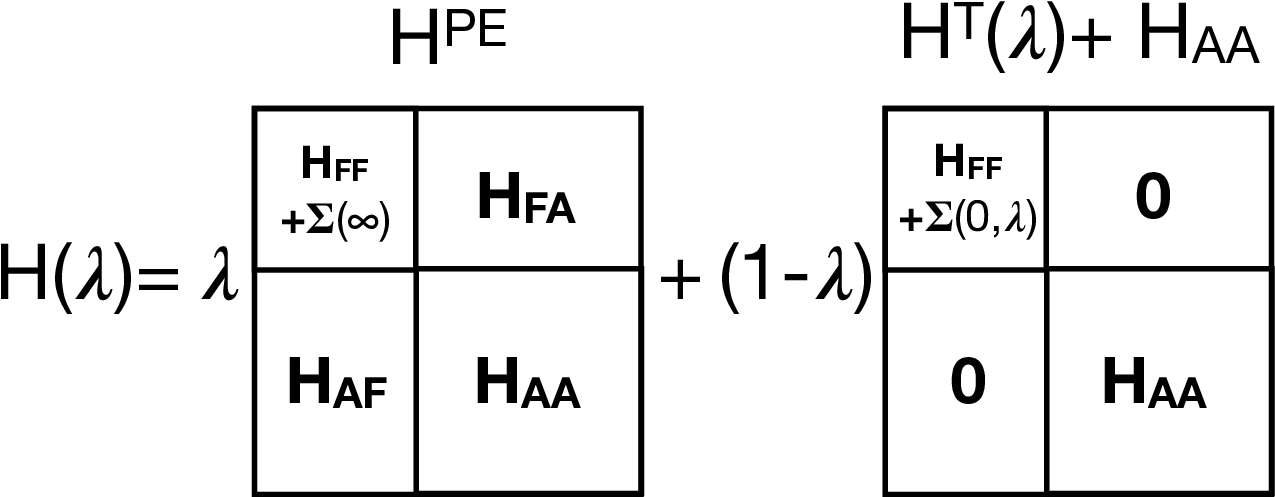
| (S.14) |
The end-point systems, i.e., the PE () and the topological Hamiltonian with detached auxiliary orbitals (), have band gaps. Since further is independent of , no band with a finite physical weight can cross the Fermi energy during the interpolation, as this would affect . The only remaining possibility to close the band gap is if a purely auxiliary band crosses the Fermi energy, i.e. that there exists an eigenvector such that and for some and . However, since has no physical () component, , see Fig. S.2. Furthermore, the auxiliary part of is identical to that of the PE Hamiltonian, , which together with gives . That is, the purely auxiliary vector must also be an eigenvector of with a zero eigenvalue. This eigenvector can not exist since the PE Hamiltonian was assumed to be insulating. This implies that no band can cross the Fermi energy during the continuous interpolation in Eq. (S.12).
The PE Hamiltonian and the combined topological auxiliary Hamiltonian are hence topologically equivalent. The topological Hamiltonian is by itself only topologically equivalent to if the detached auxiliary Hamiltonian is topologically trivial. is automatically trivial if the self-energy is local (-independent), but for a non-local self-energy it becomes necessary to consider how the auxiliary orbitals contribute to the elementary band representations Bradlyn et al. 2017, as shown by two concrete examples in the next section.

I.3 Non-local self-energy
Let us illustrate the topological role of the non-local self-energy by constructing two simple examples for which PE and topological Hamiltonian are not topologically equivalent. From the definition of the topological Hamiltonian it is clear that if is much smaller than the band gap of it cannot change the topology of . On the other hand, the auxiliary orbitals in the PE Hamiltonian may change its topology even with an infinitesimal coupling strength. Let us therefore start with a system governed by the topologically non-trivial Bernevig-Hughes-Zhang (BHZ) HamiltonianBernevig et al. 2006
| (S.15) |
and define a non-local self-energy as , where is the coupling strength. Such a self-energy can be obtained if we have a non-local and frequency-dependent interaction. The corresponding PE and topological Hamiltonians can be easily identified as
| (S.18) |
where is the identity matrix, and the second row and column in the matrix in Eq. I.3 corresponds to the auxiliary orbitals (c.f. Fig. S.1). is topologically non-trivial for all , since has the same eigenvectors as and the sign of the eigenvalues are identical. On the other hand, the reversed sign of in the auxiliary sector of makes the PE system topologically trivial for all 55 5 The physical and auxiliary orbitals form two separated non-trivial subspaces when . However, since is not considered a protected symmetry, this separation is not topological and the full system is still trivial.. This proves that the PE and topological Hamiltonian are topologically not equivalent.
This is confirmed by slab calculations, see Fig. S.3, using from Eq. (I.3) and from Eq. (S.18). These reveal the presence of metallic surface states for while the spectrum is gapped for , as expected.
Another example is given by a system with the same non-local self-energy but with the constant Hamiltonian
| (S.19) |
The corresponding PE and topological Hamiltonians become
| (S.22) |
The PE Hamiltonian of Eq. (I.3) is non-trivial if , while it becomes trivial when . The topological Hamiltonian has just the opposite classification.


These two examples clearly demonstrates the topological role of the auxiliary orbitals and the poles of the self-energy. Even when it is possible to detach the auxiliary orbitals from the physical system, their contribution to the topology cannot be neglected.
One may make an analogy to a system with spin-orbit coupling, and let the spin-up and the spin-down channel take the role of the physical and the auxiliary orbitals, respectively. Even if it would be possible to smoothly switch off the spin-orbit coupling, and hence detach the two spin channels, one can still not determine the topology of the original spin-full system (PE Hamiltonian) from the spin-up channel alone (topological Hamiltonian). Just as the topological invariants must trace over both spin channels, they must also at least formally trace over the auxiliary orbitals.
To sum up, we have proven that the PE and topological Hamiltonian are topologically equivalent for a local (e.g. DMFT) self-energy but may be topologically distinct for a non-local self-energy. Only the PE Hamiltonian properly reflects the topology of the system, whereas for a non-local self-energy the topological Hamiltonian may yield the wrong topology.
II Computational details
All the SmB6 DFT+DMFT calculations were performed using the experimental cubic crystal structure (space group: 221, prototype: CaB6) with the lattice parameter Å. The DFT exchange-correlation functional was set to the local density approximationPerdew and Wang 1992, and the Brillouin zone was sampled through a conventional Monkhorst-Pack mesh of 16 x 16 x 16 k-points in the bulk and 16 x 16 x 1 k-points in the slab calculations. The local Coulomb interaction was parameterized in terms of the Slater parameters , , , and . The Hubbard parameter is heavily screened by the valence electrons and was set to eV. The less screened Slater parameters , , and were instead calculated through Slater integrals at the beginning of each DFT iteration, and then scaled by 0.95, 0.97, and 1.00, respectively Yamaoka et al. 2012.The final self-consistent values are given in Table S.I.
The fully charge self-consistent DFT+DMFT calculation were performed using the full-potential linear muffin-tin orbital (LMTO) code RSPt Wills et al. 2000 and the DMFT implementation presented in Refs. Grechnev et al. 2007; Grånäs et al. 2012; Thunström et al. 2012. The lattice Hamiltonian as well as the DMFT lattice Green’s function are calculated in the full LMTO basis. The projection operators upon the localized Sm 4f orbitals are obtained from a -dependent Löwdin orthogonalization of the LMTO SM 4f orbitals, as detailed in the Supplemental Material of Ref. Thunström et al. 2012.
| Label | Termination | F0 | F2 | F4 | F6 | ||
|---|---|---|---|---|---|---|---|
| Sm | Bulk | 8.0 | 11.43 | 7.49 | 5.54 | 35.32 | 37.75 |
| Sm1 | Sm | 8.0 | 11.39 | 7.47 | 5.52 | 35.55 | 37.82 |
| Sm2 | Sm | 8.0 | 11.40 | 7.47 | 5.52 | 35.55 | 37.91 |
| Sm3 | Sm | 8.0 | 11.39 | 7.47 | 5.52 | 35.70 | 37.85 |
| Sm4 | Sm | 8.0 | 10.83 | 7.07 | 5.22 | 39.62 | 41.75 |
| Sm1 | B6 | 8.0 | 11.43 | 7.50 | 5.54 | 35.25 | 37.72 |
| Sm2 | B6 | 8.0 | 11.43 | 7.50 | 5.54 | 35.26 | 37.67 |
| Sm3 | B6 | 8.0 | 11.42 | 7.49 | 5.54 | 35.29 | 37.75 |
| Sm4 | B6 | 8.0 | 11.86 | 7.80 | 5.77 | 32.33 | 34.37 |
II.1 Exact diagonalization
The Sm 4f orbitals are strongly contracted compared to the Sm 5d and 6s orbitals, which makes the Sm 4f orbitals hybridize very weakly with the orbitals on neighboring atoms. The hybridization is completely captured by the local hybridization function Georges et al. 1996; Kotliar et al. 2006; Held 2007 that describes how the electrons propagate in the material once they leave the Sm 4f orbitals of a given atom. To put the weak Sm 4f hybridization in perspective, the Ni 3d hybridization function in NiO is about 20 times larger than the Sm 4f hybridization function in SmB6 for comparable computational setups. The electronic structure of SmB6 is therefore already well-described on the eV energy scale by completely neglecting the hybridization Thunström et al. 2009. However, this approach is not accurate enough to describe the important meV energy scale close to the Fermi energy. It is particularly important that the hybridization function at the Fermi energy is accurately captured, as well as the Sm 4f occupation, to ensure that the Fermi energy remains in the hybridization band gap during the DFT+DMFT self-consistency cycle. The Exact Diagonalization (ED) impurity solver Caffarel and Krauth 1994; Thunström et al. 2012; Liebsch and Ishida 2011 takes most of the hybridization between the correlated Sm 4f orbitals and the rest of the material into account by including a limited number of effective bath orbitals in the impurity problem. However, the total number of bath orbitals that can be included in the impurity problem is severely limited by the growth of the many-body Hilbert space. In order to still get an accurate representation of and the Sm 4f occupation we need to go beyond the standard hybridization fitting scheme as well as modifying the double counting correction. The details thereof are described in the next two subsections.
II.2 Bath discretization
In the self-consistent DMFT scheme the lattice Green’s function in Eq. (S.9) is projected onto the local Sm 4f orbitals () and integrated over the Brillouin zone to yield the local Green’s function . The hybridization function is then extracted from the inverse of ,
| (S.23) |
where is the local impurity Hamiltonian in Eq. (S.1) which includes the spin-orbit coupling, the double-counting, and all crystal field terms. is the local self-energy given by Eq. (S.8). The ED method proceeds by fitting a few bath state parameters and to via the model function
| (S.24) |
We fit the hybridization function on the Matsubara axis with 6 bath states per Sm orbital using a conjugate gradient scheme which also takes the off-diagonal terms in into account. The high-energy bath states (), i.e. the eigenstates of with energies relatively far from the Fermi energy (), give only a perturbative contribution to the low energy physics due to the large energy cost of exciting these bath states. Their effect can be estimated by introducing the scaling and in , which keeps invariant, and let the scaling parameter . The scaling shows that the high energy bath states can be replaced to zeroth order by a static contribution
| (S.25) |
where is the low-energy complement to , i.e. . In our calculations we put the high-energy cut-off at . The remaining low-energy bath states were ordered according to their weight , and included in to the extent allowed by the computational resources, with a minimum of 4 bath states in total. The converged one-particle term of the ED Hamiltonian for the bulk calculation is presented in Fig. S.4.
II.3 Double counting correction
In the DFT+DMFT scheme, the explicit addition of a local Coulomb interaction term to the DFT Hamiltonian introduces a double counting (DC) of the electron-electron interaction. The unknown form of the screening processes in the exchange correlation functional prevents the implementation of an exact double counting correction. In particular, the screening of the local interaction between the Sm 4f electrons, implicitly described within the local density approximation, may be different to the effective (static) screening implied by the renormalized Slater parameters. Due to this ambiguity several different double counting corrections schemes have been suggested over the years, such as the Fully Localized Limit (FLL) Solovyev et al. 1994 and Around Mean Field (AMF) Anisimov et al. 1991. The FLL correction removes the spherically averaged Hartree-Fock contribution of an effective atomic-like system with integer orbital occupations. The AMF correction considers instead an effective itinerant system with uniform (non-integer) orbital occupations. However, the thermal ground state of an intermediate valence compound such as Sm6 falls outside these two scenarios as it contains several thermally occupied almost atomic-like many-body eigenstates having different number of electrons, as shown in Table S.II. The occupation of an intermediate valence ground state responds to the DC potential in Fermi-Dirac-like steps. However, the underlying assumptions of both FLL and AMF make their DC correction linear in the occupation. The two different behaviors always lead to a feed-back loop away from intermediate valence towards integer valence. A second less sever issue is that the finite discretization of the bath states in ED causes a small mismatch between the impurity green’s function and the local green’s function projected from the lattice. To minimize these two problems we automatically adjusted the double counting potential at each DMFT iteration to obtain the same number of Sm 4f electrons in the impurity as in the lattice. In the bulk calculation the number of Sm 4f electrons stabilizes at 5.48 at a temperature of 100 K, remarkable close to the experimental value of 5.45Mizumaki et al. 2009. In the slab calculations we chose to enforce the bulk Sm 4f occupation of 5.48 for all the Sm atoms except at the surface, to make the center Sm atom as bulk-like as possible and minimize the hybridization between the surface states located at the top and bottom of the slab.
III Many-body electronic structure
III.1 Thermal ground state
| Sym | E(meV) | GS(%) | |||||||
|---|---|---|---|---|---|---|---|---|---|
| 6.002 | 0 | 46 | 0.03 | 2.95 | 2.94 | 0.00 | 0.00 | 0.00 | |
| 5.030 | 11 | 12 | 2.52 | 4.93 | 2.47 | 1.80 | 3.16 | -1.36 | |
| 5.030 | 11 | 12 | 2.52 | 4.93 | 2.47 | 0.47 | 0.75 | -0.28 | |
| 5.030 | 11 | 12 | 2.52 | 4.93 | 2.47 | -0.47 | -0.75 | 0.28 | |
| 5.030 | 11 | 12 | 2.52 | 4.93 | 2.47 | -1.80 | -3.16 | 1.36 | |
| 5.029 | 24 | 3 | 2.53 | 4.93 | 2.47 | 0.77 | 1.07 | -0.30 | |
| 5.029 | 24 | 3 | 2.53 | 4.93 | 2.47 | -0.77 | -1.07 | 0.30 | |
| 6.002 | 47 | 0 | 1.01 | 2.96 | 2.95 | -1.00 | -0.50 | -0.50 | |
| 6.002 | 47 | 0 | 1.01 | 2.96 | 2.95 | 0.00 | 0.00 | -0.00 | |
| 6.002 | 47 | 0 | 1.01 | 2.96 | 2.95 | 1.00 | 0.50 | 0.50 |
The lowest energy many-body eigenstates of the self-consistent impurity problem Hamiltonian is given in Table S.II. The states have almost atomic-like Sm 4f occupations () and total angular momenta (), but the crystal fields and the hybridization with the bath mix the different configurations. The thermal groundstate is an incoherent mixture of the eigenstates according to their Boltzmann weights (GS) at 100 K. At this temperature the largest contributions are given by the four degenerate states (48%) with and , and the state (46%) with and , in agreement with non-resonant inelastic X-ray scattering data Sundermann et al. 2018. The remaining 6% belongs to a doublet.
III.2 Extended photoemission spectrum
In Fig. 1 of the main paper, we have already shown the spectral function in a small energy range from -1.2 eV to 0.1 eV, which resolves the and multiplets for and . In Fig. S.5 we show the same -integrated spectral function in a larger energy window. Clearly all peaks agree well with the experimentally measured (on-resonance) photoemission data Denlinger et al. 2014. The relative weight of the transitions are accurately captured. The relative weight of the different transitions are in reasonable agreement with the experimental data, even though we do not include the resonance effect which strongly enhances their total weight. This gives us further assurance that our DFT+DMFT calculation faithfully describe bulk SmB6.

IV Robustness of the topological surface states
IV.1 Adding a surface potential
To numerically confirm the topological protection of the surface bands we applied time-reversal symmetric potentials to the (sub)surface layer of the Sm terminated supercell displayed to the right in Fig. S.8. The topological surface states should survive under these perturbing potentials, which can occur for example due to surface reconstructions. Our results are shown in Figs. S.6 and S.7, where we applied the potential to the and spin-orbitals of the Sm manifold, respectively. These spin-orbitals were chosen as the surface states around the -point has primarily character, while the surface states around the -point have mainly character. Technically, we simply added the potential term to the self-energy of these states after DMFT convergence (a self-consistency including this potential is beyond our illustrative purposes). Both figures show the Sm projection on the sub-surface (left panel) and subsub-surface states (right panel). Please remember that, as discussed in the main text, the surface layer itself has another Sm valence and is insulating. The topological surface states hence appear in the sub-surface layer in the unperturbed systems.
Fig. S.6 (left) clearly shows that one of the flat orbitals (i.e., the ) is shifted above the Fermi energy upon increasing the potential . At the same time, the topological surface states around the -point shift from the sub-surface layer for to the subsub-surface layer at eV. There is a crossover in-between with the surface states being extended to both layers.
At the same time the topological surface states around the -point remain on the sub-surface layer. If we instead apply a potential to the spin-orbitals as in Fig. S.7, it is these topological surface states which start to shift to the next layer below. The -pocket is however more robustly anchored to the sub-surface atom compared to the -pocket, and does not shift completely away even for eV.
The larger ”mobility” of the pocket in the spin-orbitals is interesting, as it is seen in some experiments Hlawenka et al. 2018; Jiang et al. 2013; Xu et al. 2013 but not in others Denlinger et al. 2014; Jiang et al. 2013; Xu et al. 2013. In the latter experiments, the pocket might simply hide a few layers deeper in the bulk, escaping its detection in surface-sensitive photoemission experiments.
Another possible explanation of the experimental discrepancies reveals itself at eV in Fig. S.6. At this potential strength the topologically derived -pocket and -pocket get very close to each other around the Fermi energy, and the latter can easily be misidentified as an umklapp-state Hlawenka et al. 2018; Xu et al. 2013. Interestingly, at the very same potential there are trivial bands which grace the Fermi energy close to the -point. These trivial bands may be connected to the weak -pocket seen in some experimentsHlawenka et al. 2018; Jiang et al. 2013; Xu et al. 2013. However, to put these observations on firmer ground several fully self-consistent slab calculations with various realistic surface reconstructions are needed, which is beyond the scope of current study.
| Sm 4f sub-surface | Sm 4f subsub-surface |


| Sm sub-surface | Sm subsub-surface |


IV.2 Magnetic field perpendicular to the surface
Next we apply a spin-polarizing field instead of a potential term to the surface. The field () is directed perpendicular to the surface and it breaks the time reversal symmetry of the system. The perturbation is hence expected to destroy the topological protection of the surface states. We target the same two different pairs of states as for the potential term. That is, we apply the field to the subsurface Sm 4f , and spin-orbitals. As shown in Fig. S.8, the perturbing fields indeed allow the surface states around the Fermi level to hybridize, including the otherwise protected topological surface states.
Let us start with the field applied to the spin-orbitals in Fig. S.8 (left). The large coupling between the field and the component of the surface states makes the surface bands very susceptible to the perturbing (time reversal symmetry breaking) field. The topological surface states start to hybridize and an indirect band gap opens. Quantitatively, the spectrum is altered more at the point than at the -point as here the character dominate. But also at the -point a small gap opens.
It is exactly vice versa if we apply the perturbing field to the subsurface Sm 4f , spin-orbitals, see Fig. S.8 (right). Here, actually only the topological surface state around the -point are gapped out, whereas the topological surface bands around remains intact. While applying a field to only part of the Sm states is, as a matter of course, a theoretical construct, it still demonstrates that the and pockets can clearly shift independently.