Systematic parameterization of heat-assisted magnetic recording switching probabilities and the consequences for the resulting SNR
Abstract
The signal-to-noise ratio (SNR) of a bit series written with heat-assisted magnetic recording (HAMR) on granular media depends on a large number of different parameters. The choice of material properties is essential for the obtained switching probabilities of single grains and therefore for the written bits’ quality in terms of SNR. Studies where the effects of different material compositions on transition jitter and the switching probability are evaluated were done, but it is not obvious, how significant those improvements will finally change the received SNR. To investigate that influence, we developed an analytical model of the switching probability phase diagram, which contains independent parameters for, inter alia, transition width, switching probability and curvature. Different values lead to corresponding bit patterns on granular media, where a reader model detects the resulting signal, which is finally converted to a parameter dependent SNR value. For grain diameters between 4 and 8 nm, we show an increase of ~10 dB for bit lengths between 4 and 12 nm, an increase of ~9 dB for maximum switching probabilities between 0.64 and 1.00, a decrease of ~5 dB for down-track-jitter parameters between 0 and 4 nm and an increase of ~1 dB for reduced bit curvature. Those results are furthermore compared to the theoretical formulas for the SNR. We obtain a good agreement, even though we show slight deviations.
I Introduction
The quality of a written bit pattern on granular media is mostly determined by the signal-to-noise ratio (SNR). A high SNR means low noise and a sharp edge between neighboring bits. The SNR depends either on suitable magnetic material properties of the grains to provide a good switching probability in the writing process but also on the size and position distribution of the grains in the granular medium. There are different methods to calculate the switching probability of a grain model during heat-assisted magnetic recording (HAMR), which is subject to a heat pulse and an external magnetic field. One method is solving the stochastic Landau-Lifshitz-Gilbert (LLG) equation for each atom of the grain (Ref. [1]), another is solving the stochastic coarse-grained Landau-Lifshiftz-Bloch (LLB) equation (Ref. [2]). Depending on the down-track position and off-track position , the repetition of switching trajectories for a given parameter set results in the approximate switching probability of a grain. Calculating the probability for various and yields a phase diagram of the writing process. Instead of the off-track direction , the peak temperature can be used, because then there is no need to specify the maximum temperature at the track center beforehand. For each peak temperature the off-track direction can be easily determined under the assumption of a Gaussian heat pulse via the relation
| (1) |
where and are the overall minimum and maximum temperatures of the whole heat pulse and its standard deviation. The final phase diagrams for the switching probability (as in Ref. [4, Fig.2]) allow to simulate writing processes of bit patterns on granular media as we will describe in Sec. III. The advantage of this approach is that the phase diagram has to be created only once and the switching probability can afterwards be extracted for an arbitrary amount of magnetic grains with no further computational effort. The disadvantage is that every grain is regarded individually and therefore it is not obvious how to take stray-field interactions into account. This can be done by adjusting the intrinsic distribution of the Curie temperature as shown in Ref. [3]. The phase plots contain much information about the size and characteristics of the magnetic grains as well as the parameters of the writing process (velocity, external applied field etc.). In Ref. [5] for instance, the shape of the phase diagram depending on the composition of a bi-layer material is investigated. This information only refers to a single grain but a priori tells very little about the resulting SNR of the read-back signal of a bit series. Hence, there is need to systematically investigate the influence of changes of the phase diagram on the final SNR. In this work we will develop a mathematical model of a phase diagram, which allows to vary certain parameters and perform writing processes with the resulting diagrams. The read-back signal then gives some indication of the potential SNR-improvement. The mathematical formulation of the phase plot is presented in Sec. II. In Sec. III, we will describe the simulation of the writing and read-back processes and Sec. IV will summarize and discuss the results of the received SNR and compare those to theoretical formulas.
II Mathematical model of a phase plot
In heat-assisted magnetic recording (HAMR) the switching probability of a magnetic grain can be represented as a phase diagram. As in Ref. [4, Fig. 2] the area of the highest switching probability has a C-like shape in the -plane. In the following we define an analytical function , which allows to fit such a phase plot.
II-A Model parameters
We use eight parameters that fully determine the shape of the phase plot:
- •
down-track-jitter parameter: [nm]
- •
off-track-jitter parameter: [K]
- •
maximum switching probability:
- •
half maximum temperature: [K]
- •
bit length: [nm]
- •
curvature parameter: [nm/]
- •
position in -direction: [K]
- •
position in -direction: [nm]
II-B Mathematical model
We now define the model function in three steps with two help functions and . Note that those functions depend on the upper parameters. First the down-track- and off-track-jitter is modeled as the slope of the probability function graph along a cut through the phase diagram for fixed and , respectively. As in Ref. [5, eq. (4)] we use the Gaussian cumulative distribution function
| (2) |
with
| (3) |
and determining the slope of . We write
| (4) |
and receive a function as in Fig. 1 (a) that models the down-track-jitter parameter via the vertical and the off-track-jitter parameter via the horizontal contour sharpness. The variable determines the maximum function value, i.e. the formal limit
| (5) |
When a bit is written, the switching probability should again decrease after a certain writing distance in down-track direction, therefore we additionally multiply a mirrored and shifted function in the form
| (6) |
and receive a function graph as in Fig. 1 (b). The maximum function value is but note, that this only holds in the limit for , so might never be actually reached. Finally we receive the complete model via transformation of the bit into a parabolic shape via
| (7) |
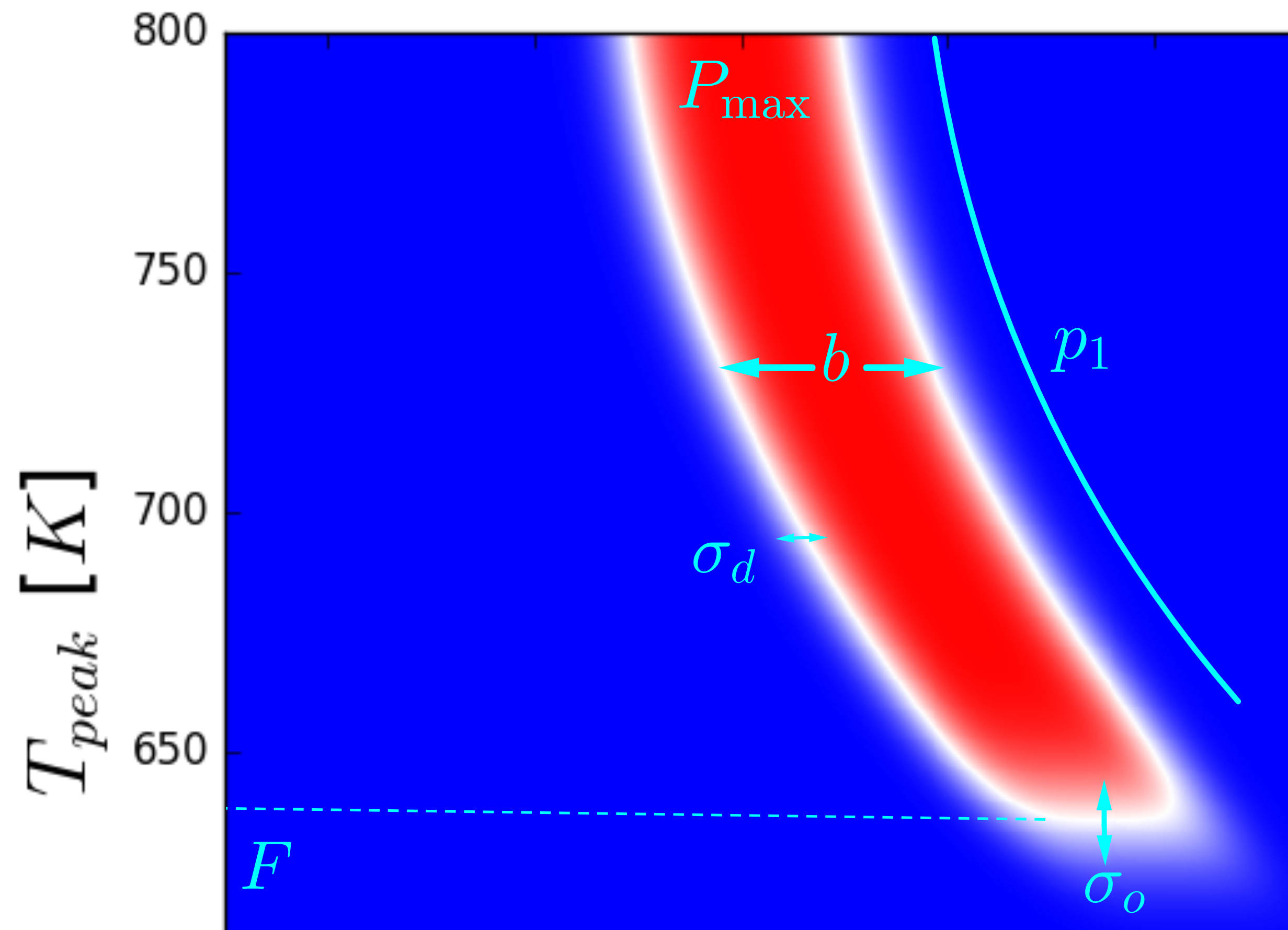
to get the C-like curvature as in Fig. 1 (c), which is usually observed (see Ref. [4, Fig.2]). The impact of the model parameters defined in Sec. II-A on the shape of the model function can be visually observed in Fig. 2.


II-C Reference system and variation of the parameters
We aim to investigate the influence of the described switching probability phase plots on the resulting SNR. Of course, it is desirable to start all variations from a realistic basic parameter set. To compute a reference phase plot, we use the LLB model as in Ref. [2] with the material parameters that can be seen in Tab. I, a grain height of nm, an applied external magnetic field of T tilted with an angle of with respect to the -direction and a duration of ns. Further a moving Gaussian heat pulse with a velocity of m/s and a full width at half maximum (FWHM) of nm, that leads to a maximum thermal gradient of K/nm, is assumed.
| [J/] | |
|---|---|
| [J/link] | |
| [] | |
| [T] | |
| [nm] | |
The resulting phase diagram for a grain diameter of nm is shown exemplarily in Fig. 3. The reference parameters of the plots in Fig. 1 are determined via a least square fit of the simulated diagram in Fig. 3. For different grain sizes the eight resulting fitted parameters according to Sec. II-A are given in Tab. II.
| grain diameter | |||||
| nm | nm | nm | nm | nm | |
| [nm] | 2.51 | 2.03 | 1.74 | 1.50 | 1.37 |
| [K] | 27.7 | 22.5 | 18.0 | 14.4 | 13.6 |
| 0.993 | 0.995 | 0.993 | 0.997 | 1.000 | |
| [K] | 571 | 602 | 617 | 628 | 639 |
| [nm] | 10.2 | 10.2 | 10.3 | 10.2 | 10.1 |
| [ nm/] | 3.28 | 3.88 | 4.33 | 4.89 | 5.16 |
| [K] | 839 | 839 | 836 | 830 | 832 |
| [nm] | 29.5 | 27.5 | 26.5 | 25.8 | 25.8 |
In Sec. IV we investigate the influence of and on the read-back SNR. The investigated parameter variations are taken in the ranges of Tab. III and in Fig. 4 (a)-(d) their influence on the phase diagram is visualized.

| parameter | min value | max value |
|---|---|---|
| [nm] | 0.01 | 4.00 |
| 0.64 | 1.00 | |
| [nm] | 4.0 | 12.0 |
| curvature reduction [%] | 0 | 100 |


III Bit patterns on granular media
III-A Writing process
We aim to use a phase plot, which determines the switching probability of a single cylindrical grain, to write bit patterns on granular media. Each medium contains approximately equally sized magnetic grains with a diameter of respectively nm. The diameter’s standard deviation of about nm is neglected in the following writing process, so we assume that each grain within the granular medium has the same size. Nonmagnetic material separates neighboring grains by nm (see Fig. 5, visualized exemplarily for a diameter of nm). We assume a Gaussian heat pulse moving across the medium with a velocity of m/s, a full width at half maximum (FWHM) of nm and a maximum temperature of K, which is slightly dependent on the Curie temperature for different grain sizes of about K (see Fig. 5). The writing process is justified due to the assumption that every grain is approximated by a cylinder with a certain diameter that is subject to the Gaussian heat pulse and a trapezoidal magnetic field. The peak temperature of the heat pulse depends on the off-track position of the grain (see Fig. 6) via Eq. 1. We neglect a spatially varying temperature within a single grain and therefore assume, that the whole grain volume receives the same temperature within the entire grain. The magnetic field is aligned according to the written pseudo random bit series of Ref. [9]:
where represents a down and an up bit (i.e. field in negative, respectively positive direction). A sequence of two or more successive down respectively up bits is summed up to one writing process with multiple bit length. The stray-field is not taken into account directly and thus different grains do not influence the switching probability of each other. Its impact is only considered via an added variation to as discussed in Ref. [3]. The writing is done by mapping the switching probabilities of the corresponding phase plot to the grains of the granular medium according to their positions. Therefore a uniformly distributed pseudo random number is created. If the probability fulfills , the magnetization of the grain is changed according to the direction of the applied field. Otherwise it remains unchanged in the previous direction. The bits in the brackets are used for padding and the remaining bits in-between represent the desired bit series. The result of the whole process is shown in Fig. 7.


III-B Reading process
The reader module is defined via its sensitivity function as discussed in Ref. [10]. It is illustrated in Fig. 8 (a). The voltage of the reader is given by the integral in Ref. [10, Eq. (1)]
| (8) |
with the reader’s sensitivity function , the media’s magnetization and a reader dependent constant . Since the magnetization is assumed to have negligible dependence on the -direction and grains have strong axial anisotropy, it degenerates to an area integral in the form
| (9) |
with a constant , which does not affect the SNR value. This integral is computed via a discrete sum over the data points of the sensitivity function, multiplied with or depending whether the data point is within a grain with magnetization in down- or up-direction or a gap. Moving the sensitivity function in nm steps across the medium gives the detected read-back signal of the whole bit pattern as shown in Fig. 8 (b).

III-C SNR calculation
By repeating the writing and reading process on different randomly initialized granular media, we are able to calculate the SNR with the methods of Ref. [9]. The readback signal of the same bit sequence on 50 different media is shown in Fig. 9.

IV Results and Discussion
IV-A SNR curves
For various parameter variations, the resulting SNR curves are plotted in Fig. 10. For selected values of the parameters, Figs. 12 - 15 visualize the corresponding bit pattern. The impact of the varied parameters on the SNR can clearly be observed. The curves describing the dependence on the bit length, and the down-track-jitter demonstrate an increase of dB for bit lengths between and nm, an increase of dB for maximum switching probabilities between and and a decrease of dB for down-track-jitter parameters between and nm. Note that for small bit lengths the reader needs a better resolution (see Fig. 8 (a)) to achieve a suitable read-back signal, therefore we scale the reader resolution in down-track direction according to the bit length in the form
| (10) |
where nm denotes the initial reader resolution (see Fig. 8 (a)) and nm is the mean initial bit length according to the phase diagram in Tab.II) . The results in Fig. 10, top show a sharp decrease of the SNR for low bit lengths, so the possible reachable linear density is limited. and are clearly two parameters with significant impact on the SNR, so it is recommendable to consider those values in terms of material optimization as in Ref. [5]. Furthermore the variation of two parameters simultaneously lead to SNR contours as in Fig. 16.
Within the chosen reference system, the bit curvature does not influence the SNR strongly ( to dB). To ensure that the SNR improvement is not limited by the reader width we scale the reader width to the track width (which can be calculated with the half maximum temperature in Tab. II and the shape of the Gaussian heat pulse in Fig. 6 and has a mean value of nm) and calculate the read-back signal again (see Fig. 11 (a) and (b)). In this way we aim to receive more improvement due to the curvature reduction effect on the edges of the writing track. However, we can see in Fig. 11 (c) that the SNR slope remains almost the same.



IV-B Comparison with theory
In Ref. [6, Eq. (2.4)] the SNR-dependence on the media magnetic transition parameter , grain size (, i.e. sum of grain diameter and nonmagnetic boundary , see Fig. 5), bit length , read-back pulse width and reader width is given by
| (11) |
As in Ref. [7, Eq. (4)], the media magnetic transition parameter can be separated into two independent parts:
- •
the down-track-jitter parameter , that originates from the probability distribution in the phase diagram
- •
the grain-jitter parameter , that comes from the grain distribution in the granular medium
The stochastic independence ensures that the total jitter of these two parts can be written as
| (12) |
The grain-jitter parameter usually depends on the mean and the variation of the grain sizes. In our simulations, we assume the distribution to be very sharp, i.e. we neglect the dependence on the variations and assume all grains to have approximately the same size . In this case only depends on and a very simplified model with square grains in Ref. [7] shows
| (13) |
Since the size of the nonmagnetic grain boundary is constant nm in our media (see Fig. 5), the grain size only depends on the grain diameter . Furthermore, the proportionality in Eq. (11) may only hold, if the read-back pulse width is chosen in a realistic ratio to the bit length . Otherwise, one might be able to increase the total SNR value just by increasing , which in general is obviously not true. Therefore, we again scale the reader resolution (which is proportional to ) with the bit length according to Eq. (10) to keep the factor in Eq. (11) constant. Finally, we note that the reader width is also kept constant. Under these assumptions, we can write the SNR value as a function of the remaining variables and a proportionality constant in the form
| (14) | ||||
For the given values for nm, nm, nm and the corresponding calculated SNR values, this function can be fitted with the fitting parameter . Note that in contrast to the plots in Fig. 10, we now choose a uniform basic parameter set for all grain diameters, namely the values for nm grain diameter in Tab. II. Otherwise, we would additionally have to consider the grain size dependent variation of parameters, which are not included in the model function in Eq. (14). We obtain the value of the fitting parameter nm and the results are shown exemplarily in Fig. 17 and 18.
The plots show that the trend of the fit agrees quite well with the actual SNR curves, however for nm and nm we obtain deviations. Taking into account the approximations in both the writing process (neglection of grain size distribution) and the derivation of the formula in Eq. (14) (simple model of square grains for Eq. (13), no dependency on etc.), those seem acceptable.
V Conclusion and Remarks
We developed an analytical model for the switching probability phase diagram of a magnetic grain in a recording medium during heat-assisted magnetic recording (HAMR). Such a phase diagram describes the switching probability of the grain depending on its down-track and off-track position and is thus very valuable to evaluate the performance of a given recording setup. The proposed model has eight input parameters, determining the bit’s position, its dimensions, its jitter in down-track and off-track direction, its curvature and the maximum switching probability in the center of the bit. By mapping the switching probabilities onto a recording medium and calculating the read-back signal with a given sensitivity function it is possible to model the whole HAMR write and read cycle with little computational effort. Additionally, due to the possibility of independent parameter variation in the model, we could investigate the influence of each parameter on the resulting signal-to-noise ratio (SNR) separately. Our results showed the impact of the bit length, curvature, maximum switching probability and down-track-jitter on the final SNR of written bit patterns. Whereas the variation of the bit length, maximum switching probability and down-track-jitter led to differences of respectively dB, we could only show a gain of about dB for the reduction of bit curvature. Furthermore, the comparison with theoretical equations led to good agreement.
Since there are considerable efforts to optimize the bit quality in HAMR containing material design and writing techniques, our approach of using an analytical model for the whole recording cycle could provide a qualitative a priori indication about the cost-benefit ratio of a recording setup in terms of the SNR with low computational effort. In addition, with the proposed model the effects of individual changes, such as the down-track jitter or the transition curvature, on the SNR can be studied separately. This is not possible with direct simulations of the write process, where only material parameters of the recording grains or write parameters of the recording head can be changed, which then has an impact on many aspects of the resulting footprint.
Acknowledgment
The authors would like to thank the Austrian Science Fund (FWF) under grant No. I2214-N20 and the ASRC/IDEMA for financial support. The computational results presented have been achieved using the Vienna Scientific Cluster (VSC). Further thanks to Stephanie Hernández for providing the SNR calculator from SEAGATE, which we gratefully used for the SNR calculation of the read-back signal and Prof. Randall Victora for providing the sensitivity function of the reader.
References
- [1] R. F. L. Evans, W. J. Fan, P. Chureemart, T. A. Ostler, M. O. A. Ellis and R. W. Chantrell, Atomistic spin model simulations of magnetic nanomaterials, J. Phys.: Condens. Matter 26, 103202 (2014),
- [2] C. Vogler, C. Abert, F. Bruckner and D. Suess, Landau-Lifshitz-Bloch equation for exchange-coupled grains, Physical Review B., Vol. 90, 214431 (2014)
- [3] C. Vogler, C. Abert, F. Bruckner, D. Suess and D. Praetorius, Areal density optimizations for heat-assisted magnetic recording of high-density media, J. Appl. Phys. 119, 223903 (2016)
- [4] C. Vogler, C. Abert, F. Bruckner, D. Suess and D. Praetorius, Heat assisted magnetic recording of bit patterned media beyond 10 Tb/in², Appl. Phys. Lett. 108, 102406 (2016)
- [5] O. Muthsam, C. Vogler, and D. Suess, Noise reduction in heat-assisted magnetic recording of bit-patterned media by optimizing a high/low Tc bilayer structure, J. Appl. Phys. 122, 213903 (2017)
- [6] G. Varvaro and F. Casoli, Ultrahigh-Desity Magnetic Recording, CRC Press (2016)
- [7] X. Wang, B. Valcu and N. Yeh, Transition width limit in magnetic recording, Appl. Phys. Lett. 94, 202508 (2009)
- [8] Y. Kubota, Y. Peng, Y. Ding et.al., Heat-Assisted Magnetic Recording’s Extensibility to High Linear and Areal Density, IEEE Transactions on Magnetics, PP (2018)
- [9] S. Hernández, P. Lu, S. Granz et.al., Using Ensemble Waveform Analysis to Compare Heat Assisted Magnetic Recording Characteristics of Modeled and Measured Signals, IEEE Transactions on Magnetics, Vol. 53, 3000406 (2017)
- [10] K. Takano, Readback Spatial Sensitivity Function by Reciprocity Principle and Media Readback Flux.” IEEE Transactions on Magnetics, Vol. 49, p. 3818-3821 (2013)
- [11] D. Weller and A. Moser, Thermal Effect Limits in Ultrahigh-Density Magnetic Recording, IEEE Transactions on Magnetics, Vol. 35, p. 4423-4439 (1999)