Quenching estimates for a non-Newtonian filtration equation with singular boundary conditions

Matthew A. Beauregard^a and Burhan Selcuk^b Address: ^aDepartment of Mathematics and Statistics, Stephen F. Austin State University, Nacogdoches, TX, 75962, USA
^bDepartment of Computer Engineering, Karabuk University, Balıklarkayası Mevkii, 78050, Turkey

Abstract

In this paper, the quenching behavior of the non-Newtonian filtration equation $(\phi(u))_{t}=(\left|u_{x}\right|^{r-2}u_{x})_{x}$ with singular boundary conditions, $u_{x}\left(0,t\right)=u^{-p}(0,t)$ , $u_{x}\left(a,t\right)=(1-u(a,t))^{-q}$ is investigated. Various conditions on the initial condition are shown to guarantee quenching at either the left or right boundary. Theoretical quenching rates and lower bounds to the quenching time are determined when $\phi(u)=u$ and $r=2$ . Numerical experiments are provided to illustrate and provide additional validation of the theoretical estimates to the quenching rates and times.

Keywords:

non-Newtonian filtration equation, singular boundary condition, quenching

1 Introduction

In this paper, we study the quenching behavior of the following nonlinear heat equation with singular boundary conditions:

\left\{\begin{array}[]{l}(\phi(u))_{t}=(\left|u_{x}\right|^{r-2}u_{x})_{x},\text{\ }0<x<a,\ 0<t<T,\\ u_{x}\left(0,t\right)=u^{-p}(0,t),\ u_{x}\left(a,t\right)=(1-u(a,t))^{-q},\ 0<t<T,\\ u\left(x,0\right)=u_{0}\left(x\right),\ 0\leq x\leq a,\end{array}\right.

(1.1)

where $\phi(s)\$ is an appropriately smooth and strictly monotone increasing function with $\phi(0)=0,\phi(1)=1\$ and $\ \phi^{\prime}(s)\leq 0$ . $p$ , $q\$ are positive constants, $r\geq 2$ and $T\leq\infty$ and the initial function $u_{0}(x)$ is a non-negative smooth function satisfying the compatibility conditions:

u_{0}^{\prime}\left(0\right)=u_{0}^{-p}(0),\ u_{0}^{\prime}\left(a\right)=(1-u_{0}(a))^{-q}\text{.}

In the case, $\phi(u)=u^{1/m}\ (0<m<1)$ , Eq. (1.1) is known as the classical non-Newtonian filtration equation that attempts to model non-stationary fluid flow through a porous medium where the tangential stress of the fluid’s displacement velocity, $u$ , has a power dependence under thermodynamic expansion and compression as a result of heat transfer [12, 13, 19]. The singular boundary flux terms represent a nonlinear radiation law at the boundary and is common to polytropic filtration equations [11, 12, 13, 19]. This mathematical model may exhibit finite-time quenching, defined as a time $T=T(u_{0})<\infty$ such that

\underset{t\rightarrow T^{-}}{\lim}\min\{u(x,t):0\leq x\leq a\}\rightarrow 0\ \text{or }\underset{t\rightarrow T^{-}}{\lim}\max\{u(x,t):0\leq x\leq a\}\rightarrow 1\text{.}

In the following, the quenching time of Eq. (1.1) is denoted as $T$ .

As is well known, when $\phi(u)=u\$ and $r=2$ , the equations reduce to the heat equation. In [15] Selcuk and Ozalp considered the problem:

\left\{\begin{array}[]{l}u_{t}=u_{xx},\text{\ }0<x<a,\ 0<t<T,\\ u_{x}\left(0,t\right)=u^{-p}(0,t),\ u_{x}\left(a,t\right)=(1-u(a,t))^{-q},\ 0<t<T,\\ u\left(x,0\right)=u_{0}\left(x\right),\ 0\leq x\leq a,\end{array}\right.

(1.2)

It shown that if $u_{0}$ satisfies $u_{xx}(x,0)\leq 0$ then $\underset{t\rightarrow T^{-}}{\lim}u(0,t)\rightarrow 0$ and $u_{t}(0,t)$ blows up in finite time and the quenching location is at $x=0$ . Likewise, it was shown that if $u_{0}$ satisfies $u_{xx}(x,0)\geq 0$ then quenching will occur at $x=a$ .

In this paper, new estimates are derived for quenching rates. In addition, we provide necessary conditions that guarantee quenching at one of the boundary locations for a more general $\phi(u)$ and $r\geq 2$ .

In the following, the initial condition may satisfy either of the two conditions:

	$\displaystyle u_{xx}(x,0)$	$\displaystyle\geq$	$\displaystyle 0,0<x<a,\ \mbox{or}$		(1.3)
	$\displaystyle u_{xx}(x,0)$	$\displaystyle\leq$	$\displaystyle 0,0<x<a,$		(1.4)

and the following condition:

u_{x}(x,0)\geq 0,0<x<a.

(1.5)

These assumptions will be shown to guarantee that quenching will occur in finite time.

Quenching problems have a long history in applied mathematics literature, dating back to pioneering work of Kawarada [10], which examines the one-dimensional heat equation with a nonlinear source term with Dirichlet boundary conditions. The Kawarada equations and extensions have been a subject of interest of both numerical [1, 8, 16] and theoretical [6, 7, 5, 14, 18, 20]. In many situations, the location that quenching occurs may be difficult to obtain. Here, the situation of a singular boundary condition enables theoretical predications to happen since the quenching location is known based on simple requirements on the initial conditions.

Chan and Yuen [5] investigated a slightly different left boundary condition:

\begin{array}[]{l}u_{t}=u_{xx},\ \text{in}\ \Omega,\\ u_{x}\left(0,t\right)=(1-u(0,t))^{-p},\ u_{x}\left(a,t\right)=(1-u(a,t))^{-q},\ 0<t<T,\\ u\left(x,0\right)=u_{0}\left(x\right),\ 0\leq u_{0}\left(x\right)<1,\ \text{in }\overset{\_}{D},\end{array}

where $a,p,q>0,T\leq\infty,D=(0,a),\Omega=D\times(0,T)$ . In [5], they showed that $x=a$ is the unique quenching point in finite time if $u_{0}$ is a lower solution, and $u_{t}$ blows up at quenching time. In [14], Selcuk and Ozalp considered the problem

\begin{array}[]{l}u_{t}=u_{xx}+(1-u)^{-p},\ 0<x<1,\ 0<t<T,\\ u_{x}\left(0,t\right)=0,\ u_{x}\left(1,t\right)=-u^{-q}(1,t),\ 0<t<T,\\ u\left(x,0\right)=u_{0}\left(x\right),\ 0<u_{0}\left(x\right)<1,\ 0\leq x\leq 1.\end{array}

They showed that $x=0\$ is the quenching point in finite time, $\lim\nolimits_{t\rightarrow T^{-}}u(0,t)\rightarrow 1$ , if $u\left(x,0\right)\$ satisfies $u_{xx}(x,0)+\left(1-u(x,0)\right)^{-p}\geq 0$ and $u_{x}(x,0)\leq 0$ . Further they showed that $\ u_{t}\$ blows up at quenching time. Furthermore, they obtained a quenching rate and a lower bound for the quenching time. In [12], Li and et.al. considered the quenching problem for non-Newtonian filtration equation with a singular boundary condition

\left\{\begin{array}[]{l}(\psi(u))_{t}=(\left|u_{x}\right|^{r-2}u_{x})_{x},\text{\ }0<x<1,\ 0<t<T,\\ u_{x}\left(0,t\right)=0,\ u_{x}\left(1,t\right)=-g(u(1,t)),\ 0<t<T,\\ u\left(x,0\right)=u_{0}\left(x\right),\ 0\leq x\leq 1,\end{array}\right.

(1.6)

where $\psi(u)$ is a monotone increasing function with $\psi(0)=0,p>1,g(u)>0,g^{\prime}(u)<0$ for $u>0$ , and $\lim_{u\rightarrow 0^{+}}g(u)=\infty$ . They showed that $x=1\$ is the only quenching point in finite time under proper conditions, Further, they obtained a quenching rate and gave an example of an application of their results.

In this paper, the quenching problem, Eq. (1.1), exhibits two types of singularity terms; the boundary outflux terms $\ u^{-p}\$ and $(1-u)^{-q}\$ as Eq. (1.2). Motivated by problems (1.2) and (1.6), we investigate the quenching behavior of Eq. (1.1). Further, in such case, several questions remain open for Eq. (1.2) in [15], in particular:

1.

What are the quenching rates?
2.

What are the estimated quenching times?

This paper is arranged as follows. In Section 2, it will be shown that the solution quenches in finite time $T$ and $\underset{t\rightarrow T^{-}}{\lim}u(a,t)\rightarrow\infty\$ or $\underset{t\rightarrow T^{-}}{\lim}u(a,t)-\infty$ blows up at quenching time at the only quenching point $x=a\$ or $x=0\$ under the conditions (1.3) or (1.4), respectively, for $r>2$ . In Section 3, quenching rates are obtained of the solution near the quenching time for $\phi(u)=u\$ and $\ r=2$ . Lower bounds to the are then given. Section 4 details the development of the finite difference numerical approximation. Section 4 provides numerical experiments that provide experimental validation to our theoretical results shown in Section 3. We highlight our main results in Section 4.

2 Quenching for the non-Newtonian filtration equation

Firstly, we rewrite Eq. (1.1) into the following form:

\left\{\begin{array}[]{l}u_{t}=B(u)(\left|u_{x}\right|^{r-2}u_{x})_{x},\text{\ }0<x<a,\ 0<t<T,\\ u_{x}\left(0,t\right)=u^{-p}(0,t),\ u_{x}\left(a,t\right)=(1-u(a,t))^{-q},\ 0<t<T,\\ u\left(x,0\right)=u_{0}\left(x\right),\ 0\leq x\leq a,\end{array}\right.

(2.1)

where $r\geq 2$ , $B(u)=1/\phi^{\prime}(u)\$ and $\phi^{\prime}(u)\neq 0\$ for $u>0$ .

Lemma 2.1.

(a)

Assume that (1.5) holds. Then, $u_{x}(x,t)>0$ in $(0,a)\times(0,T_{0})$ .
(b)

Assume that (1.4) holds. Then, $u_{t}(x,t)<0$ in $(0,a)\times(0,T_{0})$ .
(c)

Assume that (1.3) holds. Then, $u_{t}(x,t)>0$ in $(0,a)\times(0,T_{0})$ .

Proof.

(a)

Let $z(x,t)=u_{x}(x,t)$ . Then, $z(x,t)$ satisfies

\begin{array}[]{l}z_{t}=B(u)(\left|z\right|^{r-2}z)_{xx}+B^{\prime}(u)z(\left|z\right|^{r-2}z)_{x},\text{\ }0<x<a,\ 0<t<T_{0},\\ z\left(0,t\right)=u^{-p}(0,t),\ z\left(a,t\right)=(1-u(a,t))^{-q},\ 0<t<T_{0},\\ z\left(x,0\right)=u_{0}^{{}^{\prime}}(x)\text{.}\end{array}

From the Maximum Principle, it follows that $z>0$ and hence $u_{x}(x,t)>0$ in $(0,a)\times(0,T_{0})$ .

(b)

Let $w(x,t)=u_{t}(x,t)$ . Then, $w(x,t)$ satisfies on $0<x<a$ and $0<t<T_{0}$ :

\begin{array}[]{l}w_{t}=B^{\prime}(u)(\left|u_{x}\right|^{r-2}u_{x})_{x}w+(r-1)B(u)(\left|u_{x}\right|^{r-2}w_{x})_{x},\end{array}

and

\begin{array}[]{l}w_{x}\left(0,t\right)=-pu^{-p-1}(0,t)w(0,t),\ 0<t<T_{0},\\ w_{x}\left(a,t\right)=q(1-u(a,t))^{-q-1}w\left(a,t\right),\ 0<t<T_{0},\\ w\left(x,0\right)=B(u_{0}\left(x\right))\left(\left|u_{0}^{{}^{\prime}}(x)\right|^{r-2}u_{0}^{{}^{\prime}}(x)\right)_{x},0\leq x\leq a.\end{array}

From the Maximum Principle, it follows that $w<0$ and hence $u_{t}(x,t)<0$ in $(0,a)\times(0,T_{0})$ .

(c)

Similarly, $u_{0}(x)$ assumes (1.3), then from the above proof we have $u_{t}(x,t)>0$ in $(0,a)\times(0,T_{0})$ . The proof is complete.

∎

Theorem 2.2.

(a)

Assume that (1.4) and (1.5) hold. Then, the solution $u$ of Eq. (2.1) quenches at time $T$ . Then quenching occurs only at the boundary $x=0$ and $u_{t}(0,t)$ blows up at the quenching time.
(b)

Assume that (1.3) and (1.5) hold. Then, $u_{t}(x,t)>0$ in $(0,a)\times(0,T_{0})$ and there exists a finite time $T$ , such that the solution $u$ of Eq. (2.1) quenches at time $T$ . Then quenching occurs only at the boundary $x=a$ and $u_{t}(a,t)$ blows up at the quenching time.

Proof.

(a)

Assume that (1.4) holds. Then, by Lemma 2.1(b), we get $u_{t}(x,t)<0$ in $(0,a)\times(0,T_{0})$ . In addition, by (1.4):

\omega_{3}=-(1-u\left(a,0\right))^{-q(r-1)}+u^{-p(r-1)}\left(0,0\right)>0\text{.}

We shall introduce a mass function:

m_{3}\left(t\right)=\displaystyle\int_{0}^{a}\phi(u\left(x,t\right))dx,0<t<T.

Then

m_{3}^{\prime}\left(t\right)=(1-u\left(a,t\right))^{-q(r-1)}-u^{-p(r-1)}\left(0,t\right)\leq-\omega_{3},

by $u_{t}(x,t)<0\$ in $(0,a)\times(0,T_{0})$ . Thus, $m_{3}\left(t\right)\leq m_{3}(0)-\omega_{3}t$ ; which means that $m_{3}\left(T_{0}\right)=0\$ for some $T_{0},(0<T\leq T_{0})$ which means $u$ quenches in finite time.

Since $r\geq 2$ , $\phi(u)\$ is an increasing function, $u_{t}(x,t)<0$ and $u_{x}(x,t)>0\$ in $(0,a)\times(0,T_{0})$ , we get

	$\displaystyle(\phi(u))_{t}=(\left\|u_{x}\right\|^{r-2}u_{x})_{x}$	$\displaystyle\rightarrow$	$\displaystyle\phi^{\prime}(u)u_{t}=(r-1)u_{x}^{r-2}u_{xx}$
		$\displaystyle\rightarrow$	$\displaystyle u_{xx}=\frac{\phi^{\prime}(u)u_{t}}{(r-1)u_{x}^{r-2}}<0.$

Namely, $u_{x}\$ is a decreasing function and since $u_{x}(a,t)=(1-u(a,t))^{-q}>1$ , $u_{x}(x,t)>1\$ in $(0,a)\times(0,T)$ . Let $\eta\in(0,a)$ . Integrating this with respect to $x$ from $0$ to $\eta$ , we have

u(\eta,t)>u(0,t)+\eta>0\text{.}

So $u\$ does not quench in $(0,a]$ .

Suppose that $u_{t}\$ is bounded in $[0,a)\times[0,T)$ . Then there is a positive constant $M$ , $u_{t}>-M$ . Therefore,

B(u)(\left|u_{x}\right|^{r-2}u_{x})_{x}>-M.

Because of $\phi^{\prime\prime}(s)<0$ , $\phi^{\prime}(s)\$ is not increasing. So, there are $\sigma\$ and $\tau,\$ which make $0<\tau\leq v<1\$ in $[0,\sigma]\times[0,T)$ , thus, $B(u)=\frac{1}{\phi^{\prime}(u)}\geq B(\tau)$ . Thus,

	$\displaystyle(\left\|u_{x}\right\|^{r-2}u_{x})_{x}$	$\displaystyle>$	$\displaystyle\frac{-M}{B(u)}\geq\frac{-M}{B(\tau)},$
	$\displaystyle(u_{x}^{r-1})_{x}$	$\displaystyle>$	$\displaystyle\frac{-M}{B(\tau)},$

from $u_{x}(x,t)>0\$ in $(0,a)\times(0,T_{0})$ . Integrating this with respect to $x$ from $0$ to $a$ , we have

(1-u(a,t))^{-(r-1)q}-u^{-(r-1)p}(0,t)>\frac{-Ma}{B(\tau)}\text{.}

As $t\rightarrow T^{-}$ , the left-hand side tends to negative infinity, while the right-hand side is finite. This contradiction shows that $u_{t}$ blows up at the quenching time for $x=0$ .

(b)

Similarly, assume that (1.3) and (1.5) hold. From (a), we have quenching occurs only at the boundary $x=a$ and $u_{t}$ blows up at the quenching time for $x=a$ . The proof is therefore complete.

∎

3 Quenching rates of the heat equation

In this section, we investigate the case where $\phi(u)=u$ and $r=2$ and determine quenching rates and lower bounds to the quenching time under certain conditions on the initial condition in Eq. (1.2). In the following we may either assumption on the spatial derivative of the initial condition:

	$\displaystyle u_{x}(x,0)\geq\frac{x}{a}(1-u(x,0))^{-q},$		$\displaystyle~~0<x<a,~~\mbox{or}$		(3.1)
	$\displaystyle u_{x}(x,0)\geq\frac{(a-x)}{a}u^{-p}(x,0),$		$\displaystyle~~0<x<a.$		(3.2)

Theorem 3.1.

If $u_{0}(x)$ satisfies condition (1.3), that is, the initial condition is not concave down, then there exists a positive constant $C_{1}$ such that

u(a,t)\leq 1-C_{1}(T-t)^{1/(2q+2)},

for $t$ sufficiently close to the quenching time $T$ .

Proof.

Define

M(x,t)=u_{t}-\delta q(1-u)^{-q-1}u_{x},

in $[0,a]\times[\tau,T)$ where $\tau\in(0,T)\$ and $\delta$ is a positive constant to be specified later. It was shown in [15], that since $u_{t}>0$ and $u_{x}>0$ in $\left(0,a\right)\times(0,T)$ , then $M(x,t)$ satisfies

\displaystyle M_{t}-M_{xx}=\delta q(q+1)(q+2)(1-u)^{-q-3}u_{x}^{3}+2\delta q(q+1)(1-u)^{-q-2}u_{x}u_{t}>0,

for $(x,t)\in(0,a)\times(\tau,T).$ Furthermore, if $\delta$ is small enough then $M(x,\tau)\geq 0$ for $x\in[0,a]$ , and $M(0,t)>0,M(a,t)>0$ for $t\in[\tau,T)$ .

Therefore, by the maximum principle, we obtain that $M(x,t)\geq 0$ for $(x,t)\in[0,a]\times[\tau,T)$ . This means that

u_{t}(x,t)\geq\delta q(1-u)^{-q-1}u_{x}(x,t),~~(x,t)\in[0,a]\times[\tau,T)

Evaluating at $x=a$ yields,

u_{t}(a,t)\geq\delta q(1-u(a,t))^{-2q-1}.

Integrating over $t$ from $t$ to $T$ gives,

u(a,t)\leq 1-C_{1}(T-t)^{1/(2q+2)},

where $C_{1}=\left(2\delta q(q+1)\right)^{1/(2q+2)}$ . ∎

If we provide the additional condition on the spatial derivative of the initial condition then we can obtain a lower bound to the value at the right hand wall. This is encapsulated in the following theorem.

Theorem 3.2.

If $u_{0}(x)$ satisfies conditions (1.3) and (3.1) then there exist positive constant $C_{2}$ such that

u(a,t)\geq 1-C_{2}(T-t)^{1/(2q+2)},

for $t$ sufficiently close to the quenching time $T$ .

Proof.

Define

J(x,t)=u_{x}-\frac{x}{a}(1-u)^{-q},~~(x,t)\in[0,a]\times[0,T).

Then, $J(x,t)$ satisfies

J_{t}-J_{xx}=\frac{1}{a}\left(2q(1-u)^{-q-1}u_{x}+xq(q+1)(1-u)^{-q-2}u_{x}^{2}\right).

$J(x,t)$ cannot attain a negative interior minimum since $u_{x}(x,t)>0$ . On the other hand, by our condition (3.1) we have $J(x,0)\geq 0$ and

J(0,t)=u^{-p}(0,t)>0,~~J(a,t)=0,

for $a\leq 1$ and $t\in(0,T)$ . By the maximum principle, we obtain that $J(x,t)\geq 0$ for $(x,t)\in[0,1]\times[0,T)$ . Therefore,

J_{x}(a,t)=\underset{h\rightarrow 0^{+}}{\lim}\frac{J(a,t)-J(a-h,t)}{h}=\underset{h\rightarrow 0^{+}}{\lim}\frac{-J(a-h,t)}{h}\leq 0\text{.}

Subsequently,

	$\displaystyle J_{x}(a,t)$	$\displaystyle=$	$\displaystyle u_{xx}(a,t)-\frac{1}{a}(1-u(a,t))^{-q}-q(1-u(a,t))^{-2q-1}$
		$\displaystyle=$	$\displaystyle u_{t}(a,t)-\frac{1}{a}(1-u(a,t))^{-q}-q(1-u(a,t))^{-2q-1}\leq 0$

and

u_{t}(a,t)\leq\frac{(qa+1)}{a}(1-u(a,t))^{-2q-1}.

Integrating over $t$ from $t$ to $T$ yields

u(a,t)\geq 1-C_{2}(T-t)^{1/(2q+2)},

where $C_{2}=\left[\frac{(qa+1)(2q+2)}{a}\right]^{1/(2q+2)}$ . ∎

Corollary 3.1.

The results of the Theorems (3.1) and (3.2) suggest as the quenching time is approached that the quenching rate of the solution can be estimated as

u(a,t)\thicksim 1-\left(T-t\right)^{\dfrac{1}{2(q+1)}}\text{.}

Equivalently,

\dfrac{\ln(1-u(a,t))}{\ln(T-t)}\thicksim\frac{1}{2(q+1)}

In addition, a lower bound for the quenching time can be calculated. From Theorem (3.2), we have

T_{q}=\frac{a(1-u_{0}(a))^{2q+2}}{2(qa+1)(q+1)}\leq T.

In the following, we assume the initial condition satisfies condition (1.4). This condition guarantees quenching will occur at the left boundary, $x=0$ . Hence, we seek quenching estimates to the quenching rate of the solution.

Theorem 3.3.

If $u_{0}(x)$ satisfies condition $(\ref{uxxneg})$ , that is, the initial condition is not concave up, then there exists a positive constant $C_{3}$ such that

u(0,t)\geq C_{3}(T-t)^{1/(2p+2)},

for $t$ sufficiently close to the quenching time $T$ .

Proof.

Define

M(x,t)=u_{t}+\delta pu^{-p-1}u_{x},~~(x,t)\in[0,a]\times[\tau,T)

where $\tau\in(0,T)$ and $\delta$ is a positive constant to be specified later. It was shown in [15] that since $u_{t}<0$ and $u_{x}>0$ in $\left(0,a\right)\times(0,T)$ then $M(x,t)$ satisfies

M_{t}-M_{xx}=-\delta p(p+1)(p+2)u^{-p-3}u_{x}^{3}+2\delta p(p+1)u^{-p-2}u_{x}u_{t}<0,

for $(x,t)\in(0,a)\times(\tau,T).$ Furthermore, if $\delta$ is small enough, then $M(x,\tau)\leq 0$ for $x\in[0,a]$ and $M(0,t)<0,~M(a,t)<0$ for $t\in[\tau,T)$ . Therefore, by the maximum principle, we obtain that $M(x,t)\leq 0$ for $(x,t)\in[0,a]\times[\tau,T).$ Subsequently, $u_{t}(x,t)\leq-\delta pu^{-p-1}u_{x}(x,t)$ for $(x,t)\in[0,a]\times[\tau,T)$ . This means, at $x=0$ we have:

u_{t}(0,t)\leq-\delta pu^{-2p-1}(0,t).

Integrating over $t$ from $t$ to $T$ yields,

u(0,t)\geq C_{3}(T-t)^{1/(2p+2)},

where $C_{3}=\left(2\delta p(p+1)\right)^{1/(2p+2)}$ . ∎

Theorem 3.4.

If $u_{0}(x)$ satisfies both (1.3) and (3.2) then there exist positive constant $C_{4}$ such that

u(0,t)\leq C_{4}(T-t)^{1/(2p+2)},

for $t$ sufficiently close to the quenching time $T$ .

Proof.

Define

J(x,t)=u_{x}-\frac{(a-x)}{a}u^{-p},~~(x,t)\in[0,a]\times[0,T).

Then, $J(x,t)$ satisfies

J_{t}-J_{xx}=\frac{1}{a}\left(2pu^{-p-1}u_{x}+(a-x)p(p+1)(1-u)^{-p-2}u_{x}^{2}\right).

Since $u_{x}>0$ , then $J(x,t)$ cannot attain a negative interior minimum. On the other hand, by the assumed condition (3.2), then $J(x,0)\geq 0$ and

J(0,t)=0,J(a,t)=(1-u(a,t))^{-q}>0,

for $t\in(0,T)$ . Therefore, by the maximum principle, we obtain that $J(x,t)\geq 0$ for $(x,t)\in[0,1]\times[0,T)$ . As a result,

J_{x}(0,t)=\underset{h\rightarrow 0^{+}}{\lim}\frac{J(h,t)-J(0,t)}{h}=\underset{h\rightarrow 0^{+}}{\lim}\frac{J(h,t)}{h}\geq 0.

This yields

	$\displaystyle J_{x}(0,t)$	$\displaystyle=$	$\displaystyle u_{xx}(0,t)+\frac{1}{a}u^{-p}(0,t)+pu^{-2p-1}(0,t)$
		$\displaystyle=$	$\displaystyle u_{t}(0,t)+\frac{1}{a}u^{-p}(0,t)+pu^{-2p-1}(0,t)\geq 0$

and

u_{t}(0,t)\geq-\frac{(pa+1)}{a}u^{-2p-1}(0,t).

Integrating from $t$ from $t$ to $T$ gives

u(0,t)\leq C_{4}(T-t)^{1/(2p+2)},

where $C_{4}=\left[\frac{(pa+1)(2p+2)}{a}\right]^{1/(2p+2)}$ . ∎

Corollary 3.2.

The results of the Theorems (3.3) and (3.4) suggest as the quenching time is approached that the quenching rate of the solution is estimated as

u(0,t)\thicksim\left(T-t\right)^{1/(2p+2)}

Equivalently,

\dfrac{\ln(u(0,t))}{\ln(T-t)}\thicksim\frac{1}{2(p+1)}

In addition, a lower bound for the quenching time is established from Theorem (3.4), namely,

T_{p}=\frac{au_{0}(0))^{2p+2}}{2(pa+1)(p+1)}\leq T.

for quenching time $T$ .

3.1 Initial Conditions Examples

It is clear, that the estimates for the quenching rates and times rely heavily on properties of the initial condition. Here, we provide initial functions that satisfy the boundary conditions while simultaneously satisfying either conditions (1.3) and (3.1) or (1.4) and (3.2).

Consider the initial condition,

u_{0}(x)=\frac{1}{4}+4x+4x^{2},~~0\leq x\leq a.

(3.3)

where $a=1/8$ . Let $p=1$ and $q=\log_{16/3}(5)$ . Since the initial condition is concave up throughout its entire domain then clearly condition (1.3) is satisfied. In addition, a straightforward calculation shows that the left boundary condition is satisfied, namely,

u_{0}^{\prime}(0)=4=\dfrac{1}{u_{0}(0)^{p}}

At the right boundary we have $u_{0}^{\prime}\left(\frac{1}{8}\right)=5$ and

\displaystyle\dfrac{1}{\left(1-u_{0}\left(\frac{1}{8}\right)\right)^{q}}=\left(\frac{16}{3}\right)^{q}=5

In Fig. 1(a) it is seen that the condition (3.1) is satisfied.

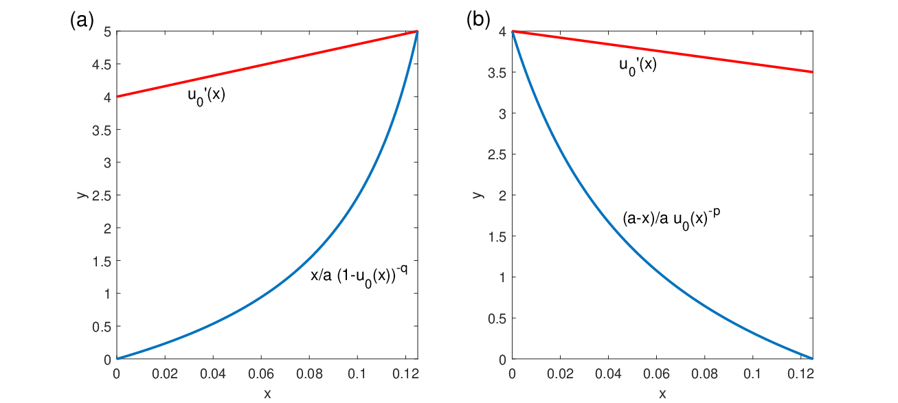
Refer to caption — Figure 1: (a) A graph of $u_{0}^{\prime}(x)$ (RED) and $\frac{x}{a}(1-u_{0}(x))^{q}$ (BLUE) for $u_{0}(x)=\frac{1}{4}-4x-4x^{2}$ . It is clear that $u_{0}^{\prime}(x)\geq\frac{x}{a}(1-u_{0}(x))^{-q}$ is satisfied throughout the domain $0\leq x\leq 1/8.$ (b) A graph of $u_{0}^{\prime}(x)$ (RED) and $\frac{a-x}{a}(u_{0}(x))^{-p}$ (BLUE) for $u_{0}(x)=\frac{1}{4}+4x-2x^{2}$ . It is clear that $u_{0}^{\prime}(x)\geq\frac{a-x}{a}(u_{0}(x))^{-p}$ is satisfied throughout the domain $0\leq x\leq 1/8.$

In light of the initial condition (3.3) then, by Corollary (3.1) we have a lower bound to quenching time. Namely:

\displaystyle T_{q}

\displaystyle=

\displaystyle\frac{\left(3/16\right)^{2q+2}}{16\left(\frac{1}{8}q+1\right)(q+1)}\approx 4.0002\times 10^{-5}.

Similarly, if the initial condition is

u_{0}(x)=\frac{1}{4}+4x-2x^{2},~~0\leq x\leq a.

(3.4)

where $a=1/8$ . Let $p=1$ and $q=\log_{32/9}\left(\frac{7}{2}\right)$ . Since the initial condition is concave down throughout its entire domain then clearly condition (1.4) is satisfied. It is clear that the left boundary condition is satisfied. At the right boundary we have $u_{0}^{\prime}\left(\frac{1}{8}\right)=\left(1-u_{0}\left(\frac{1}{8}\right)\right)^{-q}=\frac{7}{2}.$ In Fig. 1(b), we see that condition (3.2) is satisfied. Furthermore, by Corollary (3.2) we have a lower bound to quenching time. Namely:

T_{p}=\dfrac{1}{9216}\approx 1.0851\times 10^{-5}.

4 Numerical Approximation and Experiments

Let $x_{j}=jh$ for $j=0,\ldots,N+1$ and $h=a/(N+1)$ . Let $t_{k}=t_{k-1}+\tau_{k-1}$ , where $\tau_{k-1}$ is the temporal step. Let $u_{j}(t)$ be the approximation to $u(x_{j},t)$ . Define the vector $\vec{u}(t)=(u_{0}(t),u_{1}(t),\ldots,u_{N}(t),u_{N+1}(t))^{\top}$ , where $\vec{u}(0)$ is created from evaluating the initial condition at the grid points. Central difference approximations are utilized at each grid point to create the semidiscretized equations approximating Eq. (1.2), namely,

h^{2}\dot{\vec{u}}(t)=\vec{F}(\vec{u}(t)),

(4.1)

where $\vec{F}=(F_{0},\ldots,F_{N+1})$ with components defined as

F_{k}=\left\{\begin{array}[]{lcl}2u_{1}+\dfrac{2h}{(u_{0})^{p}}-2u_{0}&&k=0\\ u_{k-1}-2u_{k}+u_{k+1}&&k=1,2,\ldots,N\\ 2u_{N}+\dfrac{2h}{(1-u_{N+1})^{q}}-2u_{N+1}&&k=N+1\end{array}\right.

(4.2)

Define $\vec{v}_{m}$ as the approximation to $\vec{u}(t)$ at time $t=t_{m}$ . Then, the solution is advanced through a second order accurate Crank-Nicolson scheme [17]:

\vec{v}_{m+1}=\vec{v}_{m}+\mu_{m}(\vec{F}(\vec{v}_{m+1})+\vec{F}(\vec{v}_{m})),

(4.3)

where $\mu_{m}=\tau_{m}/(2h^{2})$ . The scheme is overall second order accurate, however, due to the singular boundary conditions the equations are stiff and it is known that unless $\tau_{k}$ is sufficiently then the method may manifest a reduction in the order of temporal convergence [9]. With this in mind, we expect the method to overall first order accurate modest temporal steps. It is common to approximate $\vec{v}_{m+1}$ in the right hand side by a first order Euler approximation, $\vec{v}_{m+1}\approx\vec{v}_{m}+2\mu_{m}\vec{F}(\vec{v}_{m})$ . This maintains the overall accuracy of the scheme will creating a semi-explicit scheme for efficiency in computations [2]. The spatial grid is fixed throughout the computation, however, adaptation may occur in the temporal step. Temporal adaption for quenching problems is critical to ensure accuracy in the quenching time. An arc-length monitoring function for $\dot{\vec{u}}$ is used to adapt the temporal step. Define

m_{i}\left(\frac{\partial u_{i}}{\partial t},t\right)=\sqrt{1+\left(\frac{\partial^{2}u_{i}}{\partial t^{2}}\right)^{2}},~~(x,t)\in[0,a]\times(0,T]

for $i=0,\ldots,N+1$ . The monitoring functions, $m_{i}$ , monitor the arc-length of the characteristic at node $x_{i}$ . Subsequently, as quenching is approached the temporal derivative grows beyond exponentially fast, therefore the arc-length will grow [3]. Therefore, we choose the temporal step such that the maximal arc-length between successive approximations at $[t_{k-2},t_{k-1}]$ and $[t_{k-1},t_{k}]$ are equivalent. Pragmatically, this leads to the equation for the temporal step:

\tau_{k}^{2}=\tau_{k-1}^{2}+\min_{i}\left\{\left[\left(\frac{\partial u_{i}}{\partial t}\right)_{k-1}-\left(\frac{\partial u_{i}}{\partial t}\right)_{k-2}\right]^{2}-\left[\left(\frac{\partial u_{i}}{\partial t}\right)_{k}-\left(\frac{\partial u_{i}}{\partial t}\right)_{k-1}\right]^{2}\right\},

for $~k=2,\ldots,$ and given the initial times steps of $\tau_{0}$ and $\tau_{1}$ .

In the following experiments, we look to verify the second order convergence rate of the numerical routine. Assume that $t\ll T$ . Let $\vec{v}_{\tau}$ be the approximation to $\vec{u}(\tau)$ for a fixed temporal step $\tau.$ Then, the maximum absolute difference between the numerical solution and $\vec{u}$ at time is $\max|\vec{v}_{\tau}-\vec{u}|\approx C\tau^{p}$ , where $C$ is some positive constant and $p$ is the order of accuracy of the temporal scheme. Consider creating a new approximation with a temporal step $\tau/2$ , then at each grid point,

	$\displaystyle\|(\vec{v}_{\tau/2}-\vec{u})_{i}\|$	$\displaystyle\approx$	$\displaystyle C\left(\dfrac{h}{2}\right)^{p}=\frac{Ch^{p}}{2^{p}}$
		$\displaystyle\approx$	$\displaystyle\frac{\|(\vec{v}_{\tau}-\vec{u})_{i}\|}{2^{p}}$

for $i=0,\ldots,N+1$ . Rearranging, yields an expression to estimate the order of accuracy,

p\approx\frac{1}{\ln(2)}\ln\left(\dfrac{|(\vec{v}_{\tau}-\vec{u})_{i}|}{|(\vec{v}_{\tau/2}-\vec{u})_{i}|}\right)

This generates an approximate convergence rate at each grid point $x_{i}$ . In the majority of applications $\vec{u}$ is unknown. Hence, a numerical solution with a relatively fine temporal step is used to estimate the rate of the underlying cauchy sequence [4].

Consider the initial condition Eq. 3.3, where $a=1/8$ , $p=1$ , and $q=\log_{16/3}(5).$ We choose $\tau=10^{-4}$ and $h=.01$ . In such case, we estimate the convergence rate of $1.013$ . Therefore, a reduction in the temporal order of convergence is manifested. To estimate the quenching time and rates, we run the simulation with $h=.001$ and $\tau_{0}=\tau_{1}=10^{-6}$ . We adapt the temporal step but require $\tau_{k}\geq 10^{-9}$ . The quenching time is numerically determined to be approximately $T\approx 1.9037\times 10^{-3}$ which is greater than our estimated lower bound of $4\times 10^{-5}.$ A loglog plot of $1-u(1/8,t)$ versus $T-t$ is shown in Fig. 2(a). A least squares approximation suggests a slope of approximately $0.253286153170844$ . The theoretical estimate was predicated to be $0.255$ .

Next, consider the initial condition Eq. 3.4, where $a=1/8$ , $p=1$ , and $q=\log_{32/9}(7/2).$ Again, we run the simulation with $h=.001$ and $\tau_{0}=\tau_{1}=10^{-6}$ . We adapt the temporal step but require $\tau_{k}\geq 10^{-9}$ . The quenching time is numerically determined to be approximately $T\approx\times 10^{-3}$ which is greater than our estimated lower bound of $1.0851\times 10^{-5}.$ A loglog plot of $u(0,t)$ versus $T-t$ is shown in Fig. 2(b). A least squares approximation suggests a slope of approximately $0.244301262418202$ . The theoretical estimate was predicated to be $0.25$ .

5 Conclusions

In this paper, a quenching problem with nonlinear boundary conditions are investigated. Certain conditions on the positivity, concavity, and the first derivative of the initial condition lead to theoretical lower bound to the quenching time, in addition to asymptotic estimates to the quenching rate. Numerical experiments provided additional validation of the pragmatic application of the theoretical analysis. We found that the experimental quenching time, $T$ , was later than our predicted lower bound. Further, the experiments suggested quenching rates that were within $1\%$ of the predicted asymptotic quenching rates.

References

[1] Beauregard, M. A., Numerical solutions to singular reaction diffusion equation over elliptical domains, Appl. Math. Comput., Vol. 254, 75-91, 2015.
[2] Beauregard, M. A., Sheng, Q., An adaptive splitting approach for the quenching solution of reaction-diffusion equations over nonuniform grids, J. Comput. Appl. Math., Vol. 241, 30-44, 2013.
[3] Beauregard, M.A., Sheng, Q., Explorations and expectations of equidistribution adaptations for nonlinear quenching problems, Adv. Appl. Math. Mech., Vol. 5, 407-422, 2013.
[4] Beauregard, M. A., Padgett, J., Parshad, R. D., A nonlinear splitting algorithm for systems of partial differential equations with self-diffusion, J. Comput. Appl. Math., Vol. 31, 8-25, 2017.
[5] Chan, C.Y., Yuen, S.I., Parabolic problems with nonlinear absorptions and releases at the boundaries, Appl. Math. Comput., 121, 203-209, 2001.
[6] C. Y. Chan and L. Ke, Parabolic quenching for nonsmooth convex domains, J. Math. Anal. Appl. 186 (1994), pp. 52-65.
[7] C. Y. Chan, A quenching criterion for a multi-dimensional parabolic problem due to a concentrated nonlinear source, J. Comput. Appl. Math., 235 (2011), pp. 3724-3727.
[8] H. Cheng, P. Lin, Q. Sheng and R.C.E. Tan, Solving degenerate reaction-diffusion equations via variable step Peaceman-Rachford splitting, SIAM J. Sci. Comput. 25 (2003), pp. 1273-1292.
[9] Hundsdorfer, W., Unconditional convergence of some Crank-Nicolson LOD method for initial-boundary value problems, Math. Comput., Vol. 58, 35-53, 1992.
[10] H. Kawarada, On solutions of initial-boundary problem for $u_{t}=u_{xx}+\frac{1}{1-u}$ , Publ. Res. Inst. Math. Sci., 10 (1975), pp. 729-736.
[11] Z. Li, C. Mu, Critical exponents for a fast diffusive polytropic filtration equation with nonlinear boundary flux, J. Math. Anal. Appl., Vol. 346, Iss. 1, pp. 55-64, 2008.
[12] X. Li, C. Mu, Q. Zhang, and S. Zhou, Quenching for a Non-Newtonian Filtration Equation with a Singular Boundary Condition, Abstr. Appl. Anal., Vol. 2012, Article ID 539161, doi:10.1155/2012/539161
[13] Y. Mi, X. Wang and C. Mu, Blow-up set for the non-Newtonian polytropic filtration equation subjected to nonlinear Neumann boundary condition, Applicable Analysis (2013) Vol. 92, No. 6, 1332–1344.
[14] Selcuk, B., Ozalp, N., The quenching behavior of a semilinear heat equation with a singular boundary outflux, Quarterly of Applied Mathematics, Vol. 72, Iss. 4, 747-752, 2014.
[15] Selcuk, B., Ozalp, N., Quenching behavior of semilinear heat equations with singular boundary conditions, Electron. J. Diff. Equ., Vol. 2015, No. 311, 1-13, 2015.
[16] Q. Sheng and A. Q. M. Khaliq, A revisit of the semi-adaptive method for singular degenerate reaction-diffusion equations, East Asia J. Appl. Math., 2 (2012), pp. 185-203.
[17] Strikwerda, John C., Finite difference schemes and partial differential equations, Wadsworth Publ. Co., Belmont, CA, ISBN: 0-534-09984, 112-134, 1989.
[18] Ozalp N, Selcuk B, The quenching behavior of a nonlinear parabolic equation with a singular parabolic with a singular boundary condition, Hacettepe Journal of Mathematics and Statistics,44: 615–621, 2015.
[19] Z. Wang, J. Yin, and C. Wang, Critical exponents of the non-Newtonian polytropic filtration equation with nonlinear boundary condition, Applied Mathematics Letters, vol. 20, no. 2, pp. 142–147, 2007.
[20] Y. Zhi, C. Mu, The quenching behavior of a nonlinear parabolic equation with a nonlinear boundary outflux, Appl. Math. Comput., 184, 624-630, 2007.