Cut–and–project quasicrystals, lattices, and dense forests

Faustin Adiceam Address: University of Manchester, United Kingdom, faustin.adiceam@manchester.ac.uk , Yaar Solomon Address: Ben-Gurion University of the Negev, Israel, yaars@bgu.ac.il and Barak Weiss Address: Tel-Aviv University, Israel, barakw@post.tau.ac.il

Abstract.

Dense forests are discrete subsets of Euclidean space which are uniformly close to all sufficiently long line segments. The degree of density of a dense forest is measured by its visibility function. We show that cut-and-project quasicrystals are never dense forests, but their finite unions could be uniformly discrete dense forests. On the other hand, we show that finite unions of lattices typically are dense forests, and give a bound on their visibility function, which is close to optimal. We also construct an explicit finite union of lattices which is a uniformly discrete dense forest with an explicit bound on its visibility.

À la mémoire d’Évariste Adiceam (1949–2018).

1. Introduction

A set $Y\subset{\mathbb{R}}^{n}$ is called uniformly discrete if there is a uniform lower bound on the distance between two distinct points of $Y$ , and of finite density if

\limsup_{T\to\infty}\frac{\#(Y\cap B(\bm{0},T))}{T^{n}}<\infty,

where $B(\bm{x},r)$ denotes the ball of radius $r>0$ around $\bm{x}\in{\mathbb{R}}^{n}$ , and the distance of points in ${\mathbb{R}}^{n}$ is measured using some norm (the precise choice of norm will be immaterial in the results that follow and we will switch between norms as convenient). Note that a uniformly discrete set is of finite density but the converse need not hold. We say that $Y$ is a dense forest if there exists a function $\varepsilon\mapsto v(\varepsilon)$ such that for every $\varepsilon>0$ , every line segment of length $v(\varepsilon)$ comes $\varepsilon$ -close to $Y$ . A function $v:{\mathbb{R}}_{+}\to{\mathbb{R}}_{+}$ for which this condition is satisfied is then referred to as a visibility function of $Y$ . By considering a disjoint collection of cylinders of round base $\varepsilon$ and height $v(\varepsilon)$ , one finds that for a dense forest of finite density, there is a constant $c>0$ such that for all $\varepsilon>0$ ,

(1.1)

v(\varepsilon)\geq c\varepsilon^{-(n-1)}.

A well-known open question of Danzer is whether there is $Y\subset{\mathbb{R}}^{2}$ which is of finite density and for which the lower bound (1.1) is sharp up to the choice of $c$ ; i.e. whether there is a dense forest in the plane of finite density with $v(\varepsilon)=O\left(\frac{1}{\varepsilon}\right)$ . Interest in Danzer’s question has led to some interest in dense forests of finite density, and uniformly discrete ones, with visibility functions which are close to the bound given by (1.1). We mention four papers which are important for our discussion. A paper of Bishop [6] gave a construction, attributed to Peres, of a dense forest of finite density in ${\mathbb{R}}^{2}$ . The construction will be reviewed below. The set in question is a union of three explicit translated lattices, and the bound $v(\varepsilon)=O\left(\varepsilon^{-4}\right)$ was given for the visibility function. The set considered in [6] is not uniformly discrete, and the first proof of the existence of a uniformly discrete dense forest was given in [21], with an explicit set in ${\mathbb{R}}^{n}$ for any $n\geq 2$ , but without an effective bound on the visibility function. In [1], for every $n\geq 2$ and every $\eta>0$ , a probabilistic construction was given which gives rise to sets of bounded density in ${\mathbb{R}}^{n}$ satisfying a visibility bound $v(\varepsilon)=O\left(\varepsilon^{-(2n-2+\eta)}\right).$ Note that in the case $n=2$ , this improves on [6], but is not yet close to (1.1). In [2], Alon gave a probabilistic argument, which showed the existence of a uniformly discrete dense forest in ${\mathbb{R}}^{2}$ with a visibility bound $v(\varepsilon)=O\left(\varepsilon^{-(1+o(1))}\right)$ . The construction of Alon could be adapted to higher dimensions as well, and yields sets which come very close to the lower bound (1.1). However the sets of [2] were not given explicitly.

Thus it is natural to search for sets $Y\subset{\mathbb{R}}^{n}$ with the following properties:

•

They are explicitly described.
•

They are uniformly discrete.
•

They are dense forests and their visibility bound comes close to (1.1).

The explicit sets we will consider involve periodic and almost periodic sets, and their finite unions. Note that a lattice is clearly uniformly discrete but is not a dense forest, and the same holds for a periodic set (a finite union of translates of one lattice). In fact a periodic set misses a neighborhood of some affine subspace of codimension one. On the other hand, as Peres showed, a union of finitely many periodic sets could be a dense forest. Such a finite union is clearly of finite density, and it is sometimes uniformly discrete (see Proposition 2.1). Another source of explicit constructions are cut-and-project sets or model sets, which are intensively studied in the literature on aperiodic structures, see e.g. [3]. We review their definition in §2.2. It is well-known that cut-and-project sets are uniformly discrete. However our first result shows that they cannot be dense forests.

Theorem 1.1.

Let $Y\subset{\mathbb{R}}^{n}$ be a cut-and-project set. Then $Y$ is not a dense forest; in fact there exists $\varepsilon>0$ and a $(n-1)$ -dimensional affine subspace $Z$ of ${\mathbb{R}}^{n}$ such that $Y$ contains no points in the $\varepsilon$ -neighborhood of $Z$ .

Nevertheless cut-and-project sets can be used to construct interesting examples of dense forests. Namely we have:

Theorem 1.2.

There exist uniformly discrete dense forests in ${\mathbb{R}}^{2},\,$ which are a finite union of cut-and-project sets.

The uniformly discrete dense forest in Theorem 1.2 is given explicitly. However our proof does not provide bounds on its visibility function. We are able to construct other sets which are finite unions of translated lattices, for which we have good visibility bounds. Namely we have:

Theorem 1.3.

There is a union of three translated lattices in ${\mathbb{R}}^{2}$ which is a uniformly discrete dense forest with visibility bound $v(\varepsilon)=O\left(\varepsilon^{-(5+\eta)}\right)$ for any $\eta>0$ .

The three translated lattices are given completely explicitly, see §6.1. Removing the condition of uniform discreteness and using more translated lattices, we are able to get much better visibility bounds:

Theorem 1.4.

For each $n\geq 2$ , each $s\geq n$ and each $\eta>0$ , for a.e. choice of $ns$ lattices in ${\mathbb{R}}^{n}$ , their union is a dense forest with visibility function satisfying

v(\varepsilon)=O\left(\varepsilon^{-(n-1+\alpha_{n}(s)+\eta)}\right),

where

\alpha_{n}(s)=\frac{n(n-1)^{2}}{s-(n-1)}\underset{s\to\infty}{\longrightarrow}0.

The measure implicit in this a.e. statement is defined by choosing at random an $s$ -tuple $\bm{\Theta}$ of vectors in ${\mathbb{R}}^{n-1}$ and applying an explicit construction described in §5.2. Moreover this a.e. set is described by the explicit condition of being uniformly Diophantine, which we introduce in this paper (see §5.3).

In the special case $n=2$ , our construction is a generalization of the construction of Peres mentioned above. Recall that Peres used a union of three explicit translated lattices to obtain a dense forest in ${\mathbb{R}}^{2}$ , see Figure 1. His argument used a Diophantine inequality to give a visibility bound of $O\left(\varepsilon^{-4}\right)$ for this set; our analysis, applied to the same set, yields a better bound of $O\left(\varepsilon^{-3}\right)$ and shows how, by choosing more lattices whose generators satisfy a different Diophantine condition, one can improve further on this bound.

\captionof

figurePeres’ construction: a union of three translated lattices in the plane which is a dense forest.

Note that all the examples considered in this paper are known not to be Danzer sets, i.e. they cannot realize the bound (1.1), see [4, 21].

Organization of the paper

After some generalities on cut-and-project constructions and tori, we prove Theorems 1.1 and 1.2 in §3 and §4 respectively. The proofs rely on viewing cut-and-project sets as return times to a section in certain higher dimensional toral flows. In §5 we introduce the condition of being uniformly Diophantine, and state Proposition 5.6, which asserts that this condition ensures a certain uniform rate of equidistribution for translations on tori. We show that such uniform equidistribution implies visibility bounds for certain finite unions of translated lattices, and thus reduce Theorems 1.3 and 1.4 to the verification of the existence of uniformly Diophantine matrices. Proposition 5.6 is proved in §6, and is used to derive Theorem 1.3. In §7 we develop a ‘metric theory’ related to the property of being uniformly Diophantine, from which we deduce the existence of the required matrices. We conclude the paper with some open problems.

Acknowledgments

The authors are grateful to the anonymous referee for helpful suggestions. They also thank the referee for producing Figure 1 and agreeing to reproduce it in this paper. The authors gratefully acknowledge the support of grants EP/T021225, BSF 2016256 and ISF 2095/15. The first named author wishes to thank Federico Ardila for a talk given at the University of Waterloo in 2018 which turned out to be most illuminating to solve some of the questions raised in this paper.

2. Preliminaries

In this section we set our notation and collect some results we will use.

2.1. Lattices

A subset $\Lambda\subset{\mathbb{R}}^{d}$ is called a lattice if there are $\bm{v}_{1},\ldots,\bm{v}_{d}$ such that $\Lambda=\mathrm{span}_{{\mathbb{Z}}}(\bm{v}_{i})={\mathbb{Z}}\bm{v}_{1}\oplus\cdots\oplus{\mathbb{Z}}\bm{v}_{d}$ (note that in this paper lattices are always of full rank). Fix a norm on ${\mathbb{R}}^{d}$ and denote by

\lambda_{1}\left(\Lambda\right)\;\leq\;\dots\;\leq\;\lambda_{d}\left(\Lambda\right)

the successive minima of $\Lambda$ ; that is, $\lambda_{k}(\Lambda)$ is the minimal $r>0$ for which $\Lambda$ contains $k$ linearly independent vectors of norm at most $r$ . The successive minima depend on the norm chosen, and unless otherwise specified, we will use the Euclidean norm. Let $\mu(\Lambda)$ denote the covering radius of $\Lambda$ ; that is,

\mu\left(\Lambda\right)\,=\;\sup_{\bm{x}\in{\mathbb{R}}^{d}}\;\inf_{\bm{\lambda}\in\Lambda}\;\left\|{\bm{x}-\bm{\lambda}}\right\|.

It then follows from Jarník’s Transference Theorem (cf. [15, Theorem 23.4 p.381]) that

(2.1)

\frac{1}{2}\cdot\lambda_{d}\left(\Lambda\right)\;\leq\;\mu\left(\Lambda\right)\;\leq\;\frac{d}{2}\cdot\lambda_{d}\left(\Lambda\right).

When using other norms, the constants $1/2,d/2$ should be replaced in (2.1) by other constants depending on the norm and on $d$ .

A translated lattice or grid is a set of the form $\bm{x}+\Lambda$ where $\Lambda$ is a lattice, and $Y\subset{\mathbb{R}}^{d}$ is called periodic if it is of the form $Y=\bigcup_{j=1}^{s}\left(\bm{x}_{j}+\Lambda\right)$ for some lattice $\Lambda$ and $\bm{x}_{j}\in{\mathbb{R}}^{d}$ .

2.2. Cut–and–project quasicrystals

We now define cut-and-project sets, which are an important source of aperiodic but ordered discrete sets in mathematical physics. For background and history we refer the reader to [3]. Let $n,k,N$ be integers with $n\geq 1,k\geq 1$ and $N=n+k$ , and write ${\mathbb{R}}^{N}=V_{phys}\oplus V_{int}$ for subspaces satisfying $\dim V_{phys}=n$ , $\dim V_{int}=k$ . The spaces $V_{phys}$ and $V_{int}$ are called the physical and the internal spaces respectively, and we denote by $\pi_{phys}:{\mathbb{R}}^{N}\to V_{phys}$ and $\pi_{int}:{\mathbb{R}}^{N}\to V_{int}$ the projections associated with the direct sum decomposition. Let $L\subset{\mathbb{R}}^{N}$ be a translated lattice, and let $W\subset V_{int}$ be a bounded set. The set

\Lambda(L,W){\,\stackrel{{\scriptstyle\mathrm{def}}}{{=}}\,}\pi_{phys}\left(L\cap\pi_{int}^{-1}(W)\right)

is called a cut-and-project set, $W$ and $L$ are its window and lattice, and $(n,N)$ are its associated dimensions.

In the literature there are two slightly different conventions regarding cut-and-project sets. In the first, one fixes $V_{phys}$ (resp. $V_{int}$ ) to be the space parallel to the first $n$ (resp. last $k$ ) coordinate axes and varies the translated lattice $L$ , while in the second, one fixes $L={\mathbb{Z}}^{N}$ and varies the summands of the direct sum decomposition ${\mathbb{R}}^{N}=V_{phys}\oplus V_{int}$ . It will be convenient for us to use both points of view. Also, in the literature, various different hypotheses are imposed on the window and on the lattice. For example it is often assumed that $W$ is compact and equal to the closure of its interior, and that $\pi_{phys}|_{L}$ is injective and $\pi_{int}(L)$ is dense. We emphasize that we do not require these assumptions and only assume that $W$ is bounded.

2.3. Tori

We will use boldface letters to denote vectors in ${\mathbb{R}}^{N}$ and write $\bm{x}\cdot\bm{y}$ for the standard inner product of $\bm{x},\bm{y}$ , $\|\bm{x}\|=\sqrt{\bm{x}\cdot\bm{x}}$ and $\bm{x}^{\perp}$ for $\{\bm{y}:\bm{x}\cdot\bm{y}=0\}$ . A torus is the quotient $V/\Lambda$ for a finite dimensional vector space $V$ and a lattice $\Lambda\subset V$ . The standard torus ${\mathbb{R}}^{N}/{\mathbb{Z}}^{N}$ will be denoted by ${\mathbb{T}}^{N}$ , and $\pi:{\mathbb{R}}^{N}\to{\mathbb{T}}^{N}$ will be the projection. For a subspace $V\subset{\mathbb{R}}^{N}$ , the restriction of the standard inner product to $V$ is an inner product, we can use this inner product to induce a volume form on $V$ , as well as on the quotient torus $T=V/\Lambda$ . For a Borel subset $A\subset T$ we denote by $\mathrm{Vol}_{T}(A)$ (or $\mathrm{Vol}(A)$ if confusion is unwarranted) its measure with respect to this volume form.

A subspace $V\subset{\mathbb{R}}^{N}$ is called rational if it is the set of solutions of a system of linear equations with rational coefficients. This happens if and only if $V\cap{\mathbb{Z}}^{N}$ is a lattice in $V$ , or equivalently, $\pi(V)$ is a torus in ${\mathbb{T}}^{N}$ . An affine subtorus of ${\mathbb{T}}^{N}$ is a translate $\bm{x}+\pi(V)$ for $V$ a rational subspace of ${\mathbb{R}}^{N}$ . Equivalently, it is a coset in the quotient ${\mathbb{T}}^{N}/\pi(V)$ . We will always equip ${\mathbb{R}}^{N}$ with the standard inner product and use its restriction to a rational subspace $V$ to equip $\pi(V)$ with a volume.

Let $V\subset{\mathbb{R}}^{N}$ be a rational subspace and $T=\pi(V)\subset{\mathbb{T}}^{N}$ be the corresponding subtorus, and denote by $\mathrm{Vol}_{T}$ the corresponding measure on $T\cong V/(V\cap{\mathbb{Z}}^{N})$ . The quotient space ${\mathbb{T}}^{N}/T$ is naturally identified with $V^{\perp}/\pi^{\perp}({\mathbb{Z}}^{N})$ where $\pi^{\perp}:{\mathbb{R}}^{N}\to V^{\perp}$ is orthogonal projection, and we let $\mathrm{Vol}_{{\mathbb{T}}^{N}/T}$ be the volume on ${\mathbb{T}}^{N}/T$ obtained by using the standard inner product on $V^{\perp}$ . With these conventions we have

(2.2)

\mathrm{Vol}_{T}(T)\cdot\mathrm{Vol}_{{\mathbb{T}}^{N}/T}\left({\mathbb{T}}^{N}/T\right)=\mathrm{Vol}\left({\mathbb{T}}^{N}\right)=1.

For a lattice $\Lambda\subset{\mathbb{R}}^{N}$ , we define its covolume to be $\mathrm{Vol}({\mathbb{R}}^{N}/\Lambda)$ , and denote this quantity by $\mathrm{coVol}(\Lambda)$ . The dual lattice of $\Lambda$ is defined by

(2.3)

\Lambda^{*}=\left\{\bm{x}\in{\mathbb{R}}^{N}:\forall\bm{y}\in\Lambda,\,\bm{x}\cdot\bm{y}\in{\mathbb{Z}}\right\},

and one has (see e.g. [13, Chap. 1])

(2.4)

\mathrm{coVol}(\Lambda)\cdot\mathrm{coVol}(\Lambda^{*})=1.

2.4. Unions of translated lattices

Understanding tori and their subtori is related to understanding closed (additive) subgroups of ${\mathbb{R}}^{N}$ . Any closed subgroup $H$ of ${\mathbb{R}}^{N}$ is of the form $H=L+V$ , where $V\subset{\mathbb{R}}^{N}$ is a vector subspace, $L$ is discrete, and the orthogonal projection of $L$ onto $V^{\perp}$ is discrete. Here $V$ is the connected component of the identity in $H$ . Recall that two discrete subgroups $L_{1},L_{2}$ are commensurable if $L_{1}\cap L_{2}$ is of finite index in both $L_{1}$ and $L_{2}$ , or equivalently, $L_{1}+L_{2}$ is discrete. Note that the connected component of $\overline{L_{1}+L_{2}}$ depends only on the commensurability class of $L_{1},L_{2}$ .

We will need the following:

Proposition 2.1.

Let $L_{1},\ldots,L_{s}$ be lattices in ${\mathbb{R}}^{N}$ . Then the following are equivalent:

(a)

There are $\bm{x}_{i},\ i=1,\ldots,s$ such that $\bigcup_{i=1}^{s}\left(\bm{x}_{i}+L_{i}\right)$ is uniformly discrete.
(b)

For each $i,j\in\{1,\ldots,s\}$ , $\overline{L_{i}-L_{j}}\neq{\mathbb{R}}^{N}$ .

Proof.

We first prove $(a)\implies(b)$ . Let $\Lambda_{i}=\bm{x}_{i}+L_{i}$ for each $i$ . Assume by contradiction that $L_{i}-L_{j}$ is dense in ${\mathbb{R}}^{N}$ . Then $\Lambda_{i}-\Lambda_{j}=L_{i}-L_{j}+\bm{x}_{i}-\bm{x}_{j}$ is also dense, and in particular for any $\varepsilon>0$ there are $\bm{x}\in\Lambda_{i},\bm{y}\in\Lambda_{j}$ such that $0<\|\bm{x}-\bm{y}\|<\varepsilon.$ This means that $\Lambda_{i}\cup\Lambda_{j}$ is not uniformly discrete.

In order to prove $(b)\implies(a)$ we will define $H_{ij}=\overline{L_{i}-L_{j}}\varsubsetneq{\mathbb{R}}^{N}$ and show that if $\bm{x}_{1},\ldots,\bm{x}_{s}$ satisfy

(2.5)

\bm{x}_{i}-\bm{x}_{j}\notin H_{ij}\text{ for all }i,j,

then $\bigcup_{i=1}^{s}\left(\bm{x}_{i}+L_{i}\right)$ is uniformly discrete. Note that (2.5) holds for almost every choice of $\bm{x}_{1},\ldots,\bm{x}_{s}$ . Let $\varepsilon>0$ be smaller than the minimal distance between $\bm{x}_{i}-\bm{x}_{j}$ and $H_{ij}$ , and also smaller than the minimal distance between two distinct points in the same $L_{i}$ . Let $\bm{y}_{1},\bm{y}_{2}$ be two distinct elements of $\bigcup_{i=1}^{s}\Lambda_{i}$ . If $\bm{y}_{1},\bm{y}_{2}$ belong to the same $\Lambda_{i}$ then they are at least a distance $\varepsilon$ apart, and otherwise we can write $\bm{y}_{1}=\bm{x}_{i^{\prime}}+\ell_{1},\ \bm{y}_{2}=\bm{x}_{j^{\prime}}+\ell_{2}$ with $i^{\prime}\neq j^{\prime}$ , $\ell_{1}\in L_{i^{\prime}}$ and $\ell_{2}\in L_{j^{\prime}}$ . Then $\ell_{2}-\ell_{1}\in H_{i^{\prime}j^{\prime}}$ and hence

\|\bm{y}_{1}-\bm{y}_{2}\|\geq\|\bm{x}_{i^{\prime}}-\bm{x}_{j^{\prime}}-(\ell_{2}-\ell_{1})\|\geq\varepsilon,

as required. ∎

Corollary 2.2.

For any two translated lattices $\Lambda_{1},\Lambda_{2}\subset{\mathbb{R}}^{N}$ , if the union $Y=\Lambda_{1}\cup\Lambda_{2}$ is uniformly discrete, then $Y$ is not a dense forest; in fact there exists $\varepsilon>0$ and an $(N-1)$ -dimensional affine subspace $Z\subset{\mathbb{R}}^{N}$ such that $Y$ contains no points in the $\varepsilon$ -neighborhood of $Z$ .

Proof.

Let $\Lambda_{i}=L_{i}+\bm{x}_{i},\ i=1,2$ , let $H=\overline{L_{1}-L_{2}}$ , and let $V$ be the connected component of the identity in $H$ . Since $Y$ is uniformly discrete, we have by Proposition 2.1 that $V\varsubsetneq{\mathbb{R}}^{N}$ . Let $V_{0}$ be an $(N-1)$ -dimensional subspace of ${\mathbb{R}}^{N}$ containing $V$ which is spanned by elements of $H$ , and let $P:{\mathbb{R}}^{N}\to V_{0}^{\perp}$ be the orthogonal projection. Then the choice of $V_{0}$ ensures that $P(H)$ is discrete, and since $L_{1}\cup L_{2}\subset H$ , we have that $Y\subset(\bm{x}_{1}+H)\cup(\bm{x}_{2}+H)$ . If we take a point $\bm{z}\in V_{0}^{\perp}\setminus P\left((\bm{x}_{1}+H)\cup(\bm{x}_{2}+H)\right)$ , then the conclusion of the Corollary will be valid with $Z=P^{-1}(\bm{z})$ . ∎

Note that by Theorem 1.3, it is possible to obtain a uniformly discrete dense forest as a union of three translated lattices in ${\mathbb{R}}^{2}$ .

2.5. Visit times in a dynamical system

Cut-and-project sets also arise as the set of visit times to a section of an ${\mathbb{R}}^{n}$ -action on ${\mathbb{T}}^{N}$ , $n<N$ . Let $V\cong{\mathbb{R}}^{n}$ be a subspace of ${\mathbb{R}}^{N}$ . Then $V$ acts on ${\mathbb{T}}^{N}$ via the linear action

\bm{v}\cdot\bm{x}=\bm{x}+\pi(\bm{v}).

Following the terminology in [16], for $\bm{x}_{0}\in{\mathbb{T}}^{N}$ and $\mathcal{S}\subset{\mathbb{T}}^{N}$ we define the $(n,N)$ -toral dynamics set by the set of ‘return times’ to $\mathcal{S}$ :

(2.6)

Y_{\mathcal{S},\bm{x}_{0}}{\,\stackrel{{\scriptstyle\mathrm{def}}}{{=}}\,}\{\bm{v}\in V:\bm{v}\cdot\bm{x}_{0}\in\mathcal{S}\}.

An ${\mathbb{R}}^{n}$ -action is called minimal if all orbits are dense. It is well-known (see e.g. [14, Chap. 3]) that the above ${\mathbb{R}}^{n}$ -action is minimal if and only if $V$ is a totally irrational subspace; namely, if and only if it is contained in no proper rational subspaces of ${\mathbb{R}}^{N}$ . Moreover, for any $\bm{x}\in{\mathbb{T}}^{N}$ , the closure $\overline{V\cdot\bm{x}}$ is an affine subtorus of ${\mathbb{T}}^{N}$ on which the $V$ -action is minimal; that is $\overline{V\cdot\bm{x}}=\bm{x}+\pi(U)$ , where $U$ is the smallest rational subspace containing $V$ .

A subset $\mathcal{S}\subset{\mathbb{T}}^{N}$ is called a linear section (for the $V$ -action on ${\mathbb{T}}^{N}$ ) if $\mathcal{S}=\pi(K)$ for a bounded set $K\subset U$ , where $U$ is a $k$ -dimensional affine subspace of ${\mathbb{R}}^{N}$ that is transverse to $V$ , and $K$ has non-empty interior in $U$ .

We will repeatedly use the following well-known fact (which was mentioned without proof in [16]):

Proposition 2.3.

If $U,V$ are subspaces of ${\mathbb{R}}^{N}$ with ${\mathbb{R}}^{N}=U\oplus V$ , and $\mathcal{S}\subset\pi(U)$ is a linear section for the associated $V$ -action on ${\mathbb{T}}^{N}$ , then for any $\bm{x_{0}}\in{\mathbb{T}}^{N}$ , the set $Y_{\mathcal{S},\bm{x_{0}}}$ is a cut-and-project set for a decomposition in which $V=V_{phys}$ and $U=V_{int}$ . Moreover any cut-and-project set arises in this way.

Proof.

Let

\bm{x}_{0}\in{\mathbb{T}}^{N},\ V=V_{phys},\ U=V_{int},\ L=-\bm{x}_{0}+{\mathbb{Z}}^{N},\ \mathcal{S}=\pi(K),\ W=-K.

Then

\begin{split}\bm{v}\in Y_{\mathcal{S},\bm{x}_{0}}\iff&\bm{v}+\bm{x}_{0}\in\mathcal{S}=\pi(K)\\ \iff&\exists\bm{w}\in W\text{ such that }\bm{v}+\pi(\bm{x}_{0})=\pi(-\bm{w})\\ \iff&\exists\bm{z}\in{\mathbb{Z}}^{N},\,\bm{w}\in W\text{ such that }v+\bm{x}_{0}=-\bm{w}+\bm{z}\\ \iff&\exists\bm{z^{\prime}}\in L,\,\bm{w}\in W\text{ such that }v+\bm{w}=\bm{z}^{\prime}\\ \iff&\exists\bm{z}^{\prime}\in L\text{ such that }\bm{v}=\pi_{phys}(\bm{z}^{\prime}),\,\pi_{int}(\bm{z}^{\prime})\in W.\end{split}

∎

2.6. More detailed statements

Via Proposition 2.3, we see that Theorem 1.1 asserts that $(n,N)$ toral dynamics sets arising from linear sections are not dense forests. On the other hand, in [21], a uniformly discrete dense forest was constructed, using visit times to a section in an ${\mathbb{R}}^{n}$ -action on a compact homogeneous space. We would like to modify this construction and use dynamics of linear toral flows instead, but as Theorem 1.1 shows, if we use a linear section the resulting set will not be a dense forest. To rectify this we will allow a larger class of sets to serve as the section $\mathcal{S}$ .

For this discussion we will specialize to the case $N=3,\,n=2$ , so that a section is one-dimensional. We say that $\mathcal{S}\subset{\mathbb{T}}^{3}$ is a piecewise linear unavoidable section if

(1)

$\mathcal{S}$ is a finite union $J_{1}\cup\cdots\cup J_{\ell}$ where the $J_{i}$ are disjoint projections under $\pi$ of closed line segments in ${\mathbb{R}}^{3}$ (of finite length).
(2)

$\mathcal{S}$ intersects every co-dimension 1 sub-torus, that is $\mathcal{S}\cap\pi(\bm{x}+Q)\neq\varnothing$ for every $\bm{x}\in{\mathbb{R}}^{3}$ and every $2$ -dimensional rational subspace $Q\subset{\mathbb{R}}^{3}$ .

The following results will be proved in §4. They immediately imply Theorem 1.2.

Theorem 2.4.

Piecewise linear unavoidable sections in ${\mathbb{T}}^{3}$ exist.

In fact, as we will see, they exist whenever the dimensions $n,N$ satisfy $N=n+1$ , but we will not be using this fact.

Theorem 2.5.

For every piecewise linear unavoidable section $\mathcal{S}\subset{\mathbb{T}}^{3}$ , every $\bm{x}_{0}\in{\mathbb{T}}^{3}$ , and every $2$ -dimensional subspace $V\subset{\mathbb{R}}^{3}$ which does not contain rational lines and is transverse to $\mathcal{S}$ , the set

Y=Y_{V,\mathcal{S},\bm{x}_{0}}{\,\stackrel{{\scriptstyle\mathrm{def}}}{{=}}\,}\left\{\bm{v}\in V:\bm{v}\cdot\bm{x}_{0}\in\mathcal{S}\right\}

is a uniformly discrete dense forest in $V\cong{\mathbb{R}}^{2}$ . The set $Y$ is a finite union of cut-and-project sets with associated dimensions $(2,3)$ , with the same physical space $V_{phys}=V$ .

See Figure 1 for an illustration (provided by the anonymous referee of this paper) of a visit set to a piecewise linear unavoidable section for the flow induced by a random plane $V$ , on $\mathbb{T}^{3}$ .

Figure 1. A visit set to a piecewise linear unavoidable section.

3. Cut-and-project sets are not dense forests

In this section we will prove Theorem 1.1. We will need the following well-known fact (see e.g. [13, Cor., p. 25]):

Proposition 3.1.

Let $\bm{q}\in{\mathbb{Z}}^{N}$ and $Q=\bm{q}^{\perp}$ . Then

(3.1)

\left\|{\bm{q}}\right\|\geq\mathrm{Vol}\left(Q/Q\cap{\mathbb{Z}}^{N}\right).

Moreover, if $\bm{q}$ is primitive (i.e. the gcd of its coordinates is equal to 1), then we have equality in (3.1).

Lemma 3.2.

Let $k,N\in{\mathbb{N}},1\leq k<N$ , and let $U\subset{\mathbb{R}}^{N}$ be a $k$ -dimensional subspace. Then for every bounded set $K\subset U$ there exists an $(N-1)$ -dimensional rational subspace $Q\subset{\mathbb{R}}^{N}$ , and some $\bm{b}\in{\mathbb{R}}^{N}$ , such that $\pi(K)\cap\pi(Q+\bm{b})=\varnothing$ .

Proof.

Given $K$ and $U$ , it suffices to find a rational subspace $Q$ of dimension $N-1$ , and a coset of $\pi(Q)$ , $\widetilde{Q}\in{\mathbb{T}}^{N}/\pi(Q)$ , such that $\pi(K)\cap\widetilde{Q}=\varnothing$ (where the quotient denotes quotients of abelian groups). Indeed, if this happens then any $\bm{b}\in\pi^{-1}(\pi(\widetilde{Q}))$ will satisfy the required conclusion. Given a rational subspace $Q\subset{\mathbb{R}}^{N}$ of dimension $N-1$ , let $P_{Q^{\perp}}:{\mathbb{R}}^{N}\to Q^{\perp}$ denote the orthogonal projection on $Q^{\perp}$ . Note that $\pi(Q)\cong Q/\left(Q\cap{\mathbb{Z}}^{N}\right)$ is an $(N-1)$ -dimensional sub-torus of ${\mathbb{T}}^{N}$ , and that the space of cosets ${\mathbb{T}}^{N}/\pi(Q)$ is parameterized by $Q^{\perp}/P_{Q^{\perp}}({\mathbb{Z}}^{N})$ .

If no such coset $\widetilde{Q}\in{\mathbb{T}}^{N}/\pi(Q)$ exists then $P_{Q^{\perp}}(K)$ covers $Q^{\perp}/P_{Q^{\perp}}({\mathbb{Z}}^{N})$ , and in particular $\mathrm{Vol}(P_{Q^{\perp}}(K))\geq\mathrm{Vol}(Q^{\perp}/P_{Q^{\perp}}({\mathbb{Z}}^{N}))$ . So it suffices to find a rational subspace $Q$ with the property that

(3.2)

\mathrm{Vol}(P_{Q^{\perp}}(K))<\mathrm{Vol}(Q^{\perp}/P_{Q^{\perp}}({\mathbb{Z}}^{N}))\stackrel{{\scriptstyle\eqref{eq: reciprocal}}}{{=}}\frac{1}{\mathrm{Vol}(Q/Q\cap{\mathbb{Z}}^{N})}\cdotp

Let $\{\bm{u}_{1},\ldots,\bm{u}_{k}\}$ be an orthonormal basis of $U$ . By replacing $K$ with a set that contains it, it suffices to find $Q$ satisfying (3.2) where

(3.3)

K=\left\{\sum_{i=1}^{k}a_{i}\bm{u}_{i}:|a_{i}|\leq t\right\},

for some $t>0$ . We will look for $Q=\mathrm{span}\,\{\bm{q}\}^{\perp}$ , where $\bm{q}\in{\mathbb{Z}}^{N}$ . By Proposition 3.1, it would suffice to find $\bm{q}\in{\mathbb{Z}}^{N}$ with $\mathrm{Vol}(P_{Q^{\perp}}(K))<\frac{1}{\left\|{\bm{q}}\right\|}$ . For $K$ as in (3.3), denoting by $\left(\bm{e}_{1},\dots,\bm{e}_{N}\right)$ the standard basis, we have

\mathrm{Vol}(P_{Q^{\perp}}(K))\leq 2\sqrt{k}\cdot t\cdot\max\left\{\left|\bm{e}_{i}\cdot{\frac{\bm{q}}{\left\|{\bm{q}}\right\|}}\right|:i\in\{1,\ldots,k\}\right\},

and this expression is smaller than $1/\left\|{\bm{q}}\right\|$ if

(3.4)

\max_{1\leq i\leq k}\left\{\left|\bm{e}_{i}\cdot{\bm{q}}\right|\right\}<\delta,\ \ \text{ where }\delta{\,\stackrel{{\scriptstyle\mathrm{def}}}{{=}}\,}\frac{1}{2\sqrt{k}t}\cdot

Let $L$ be a line in $U^{\perp}$ ; then (3.4) clearly holds if $\bm{q}$ is a nonzero integer vector in the $\delta$ -neighborhood of $L$ ; that is, in the set

\mathcal{C}{\,\stackrel{{\scriptstyle\mathrm{def}}}{{=}}\,}\left\{\bm{x}\in{\mathbb{R}}^{N}:\mathrm{dist}(\bm{x},L)<\delta\right\}.

Since $\mathcal{C}$ is a convex centrally symmetric body of infinite volume, by Minkowski’s convex body theorem (see e.g. [13, p. 71]) such an integer vector $\bm{q}$ exists. ∎

Proof of Theorem 1.1.

Replacing ${\mathbb{T}}^{N}$ if necessary with $\overline{V\cdot\bm{x}}$ , we may assume that $V$ is totally irrational. If $n=N$ then $Y$ is periodic, that is $Y$ is a finite union of cosets of a lattice $\Lambda\subset{\mathbb{R}}^{n}$ , and then we may take $Z$ to be parallel to an $(n-1)$ -dimensional subspace spanned by vectors in $\Lambda$ .

So we can assume that $n<N$ and $Y_{\mathcal{S},\bm{x}_{0}}$ is a $(n,N)$ -toral dynamics set, associated with the action of a totally irrational $n$ -dimensional space $V$ on the torus ${\mathbb{T}}^{N}$ . Set $k=N-n$ . Then, by assumption, $\mathcal{S}=\pi(K)$ , where $K$ is a compact subset of a $k$ -dimensional affine space $U\subset{\mathbb{R}}^{N}$ . Let $\bm{z}\in U\cap V$ , and note that $Y_{\mathcal{S},\bm{x}_{0}}-\bm{z}=Y_{\pi(K-\bm{z}),\bm{x}_{0}}$ . Then it suffices to show that $Y_{\pi(K-\bm{z}),\bm{x}_{0}}$ is not a dense forest. Note that $K-\bm{z}\subset U-\bm{z}$ which is a $k$ -dimensional subspace of ${\mathbb{R}}^{N}$ . By Lemma 3.2 there exists an $(N-1)$ -dimensional rational subspace $Q\subset{\mathbb{R}}^{N}$ , and a coset $\widetilde{Q}$ of it, such that $\pi(K-\bm{z})\cap\pi(\widetilde{Q})=\varnothing$ . Note that $Z{\,\stackrel{{\scriptstyle\mathrm{def}}}{{=}}\,}V\cap\widetilde{Q}$ is a $(n-1)$ -dimensional affine subspace of $V$ and of $\widetilde{Q}$ . Since $\pi(K-\bm{z})\cap\pi(\widetilde{Q})=\varnothing$ , and the sets $\pi(K-\bm{z})$ and $\pi(\widetilde{Q})$ are closed in ${\mathbb{T}}^{N}$ , there exists some $\varepsilon>0$ such that $d_{{\mathbb{T}}^{N}}(\pi(K-\bm{z}),\pi(\widetilde{Q}))>\varepsilon$ . Then we also have $d(\pi(K-\bm{z}),\pi(Z))>\varepsilon$ . That is, any point which is $\varepsilon$ -close to $Z$ misses $Y_{\mathcal{S},\bm{x}_{0}}-\bm{z}$ , and this proves the assertion. ∎

4. An explicit uniformly discrete dense forest using toral flows

In this section we will prove Theorems 2.4 and 2.5.

In order to see that a piecewise linearly unavoidable section exists, we refer the reader to Figure 2.

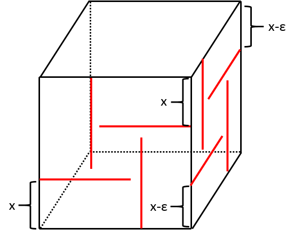
Refer to caption — Figure 2. A piecewise linearly unavoidable section in ${\mathbb{T}}^{3}$ : any 2-torus intersects at least one of the faces of the cube in a loop, and thus intersects the section.

We also sketch an alternative existence proof for linearly unavoidable sections, which uses toral dynamics and can be generalized to higher dimensions, i.e. to the case $N=n+1$ for arbitrary $n\geq 2$ .

Sketch of another proof of Theorem 2.4.

Let $\{T_{j}:j\in{\mathbb{N}}\}$ be an enumeration of the 2-dimensional affine tori passing through the origin in ${\mathbb{T}}^{3}$ . From Proposition 3.1 we have $\mathrm{Vol}(T_{j})\to\infty$ and from (2.2), $\mathrm{Vol}\left({\mathbb{T}}^{N}/T_{j}\right)\to 0$ . Let $J_{1},J_{2},J_{3}\subset{\mathbb{R}}^{3}$ be closed line segments, in linearly independent directions, such that the images in $\mathcal{S}=\bigcup\pi(J_{i})$ are disjoint. Since the directions are linearly independent, there is a uniform lower bound on the angle that each $T_{j}$ makes with at least one of the $J_{i}$ . Therefore when projecting onto ${\mathbb{T}}^{3}/T_{j}$ , for all large enough $j$ , at least one of the $J_{i}$ projects onto the quotient ${\mathbb{T}}^{3}/T_{j}$ . Thus for all sufficiently large $j$ , and every coset $T^{\prime}_{j}$ of $T_{j}$ , we have $T^{\prime}_{j}\cap\mathcal{S}\neq\varnothing$ .

Now by adding finitely many line segments to $\mathcal{S}$ , and keeping the property $\pi(J_{i_{1}})\cap\pi(J_{i_{2}})=\varnothing$ , we obtain a piecewise linear unavoidable section.∎

Proof of Theorem 2.5.

This is very close to the argument of [21, Proof of Thm. 1.3]. First note that uniform discreteness of $Y$ follows from the fact that the segments comprising $\mathcal{S}$ are closed and disjoint, and the transversality assumption. We prove that $Y$ is a dense forest by contradiction. If not, then there exists some $\varepsilon>0$ , unit vectors $\bm{w}_{j}\in V$ , and $L_{j}\to\infty$ such that the line segments $\ell_{j}{\,\stackrel{{\scriptstyle\mathrm{def}}}{{=}}\,}\{\bm{x}_{j}+t\cdot\bm{w}_{j}:t\in[0,L_{j}]\}$ satisfy $\mathrm{dist}(Y,\ell_{j})\geq\varepsilon$ for all $j$ . Denote

K_{j}{\,\stackrel{{\scriptstyle\mathrm{def}}}{{=}}\,}\left\{\bm{v}\in V:\mathrm{dist}(\bm{v},\ell_{j})\leq\frac{\varepsilon}{3}\right\},

and define a sequence of Borel probability measures $\mu_{j}$ on ${\mathbb{T}}^{3}$ by

\forall f\in C({\mathbb{T}}^{3}),\quad\int_{{\mathbb{T}}^{3}}fd\mu_{j}{\,\stackrel{{\scriptstyle\mathrm{def}}}{{=}}\,}\frac{1}{\mathrm{Vol}(K_{j})}\int_{K_{j}}f(\bm{v}\cdot\bm{x}_{0})dv,

where the integral on the right hand side is with respect to the Euclidean volume on $V$ . By passing to a subsequence we may assume that $\bm{w}_{j}\xrightarrow{j\to\infty}\bm{w}$ , and that $\mu_{j}\xrightarrow{weak-*}\mu$ . Since $\bm{w}_{j}$ is the direction of the long axis of the cylinder $K_{j}$ , and since the stabilizer of a measure is a group, it follows that the measure $\mu$ is invariant under $H{\,\stackrel{{\scriptstyle\mathrm{def}}}{{=}}\,}\mathrm{span}(\bm{w})$ . By [14, Chap. 3], every Borel probability measure on ${\mathbb{T}}^{3}$ , invariant and ergodic under $H$ , is the Haar measure on some rational torus $T\subset{\mathbb{T}}^{3}$ . Note that such a $T$ cannot be $1$ -dimensional. Indeed if such a $T$ is $1$ -dimensional then $T=\pi(H)$ , hence $\bm{w}$ is a rational direction in the physical space $V$ , contradicting the assumption that $V$ does not contain rational lines.

Let $g\in C({\mathbb{T}}^{3})$ be a bump function that is positive on $\mathcal{S}$ and supported on the $\varepsilon/3$ neighborhood of $\mathcal{S}$ . Recall that since $\mathcal{S}$ is a piecewise linear unavoidable section, $\mathcal{S}$ intersects every $2$ -dimensional rational sub-torus of ${\mathbb{T}}^{3}$ , and in particular $\mathcal{S}\cap T\neq\varnothing$ , for every $T$ as above. This implies that $\int_{{\mathbb{T}}^{3}}gd\nu>0$ for any ergodic $H$ -invariant measure $\nu$ , and hence by ergodic decomposition, $\int_{{\mathbb{T}}^{3}}gd\mu>0$ . On the other hand, for every $j$ and for every $v\in K_{j}$ , by definition $\mathrm{dist}(v,Y)\geq\frac{2\varepsilon}{3}$ , thus $\mathrm{dist}_{{\mathbb{T}}^{3}}(\bm{v}\cdot\bm{x}_{0},\mathcal{S})\geq\frac{2\varepsilon}{3}$ and $\bm{v}\cdot\bm{x}_{0}$ misses the support of $g$ . This implies $g(\bm{v}\cdot\bm{x}_{0})=0$ , and hence $\int_{{\mathbb{T}}^{3}}gd\mu_{j}=0$ for every $j$ , a contradiction to $\mu_{j}\xrightarrow{weak-*}\mu$ .

Let $I_{1},\ldots,I_{\ell}$ be line segments whose projections define $\mathcal{S}$ . Then each $\pi(I_{i})$ is a linear section and hence the set $Y=\bigcup_{j=1}^{\ell}Y_{\pi(I_{i}),\bm{x}_{0}}$ is a finite union of cut-and-project sets as required. ∎

5. Finite unions of translated lattices and uniformly Diophantine sets of vectors

We now move to results concerning finite unions of translated lattices.

5.1. More notation.

The following notation will be used in the rest of the paper. Given two expressions $X$ and $Y$ , we will use both of the notations $X\ll Y$ and $X=O(Y)$ to mean that $X$ and $Y$ are depending on some variables and there exists a constant $c>0$ (called the implicit constant), independent of these parameters, such that $X\leq cY$ .

•

Throughout we will have two dimensions $n$ and $d$ linked by the relation

$n=d+1\geq 2.$
•

The coordinates of $\bm{x}\in{\mathbb{R}}^{n}$ will be denoted by $(x_{1},\ldots,x_{n})$ .
•

$\|\cdot\|_{\infty}$ and $\|\cdot\|_{2}$ will denote respectively the sup-norm and Euclidean norm, $B_{\infty}(\bm{x},r)$ and $B_{2}(\bm{x},r)$ will denote the respective open balls. When making a statement which does not depend on the choice of norm we will simply write $\|\cdot\|$ and $B(\bm{x},r)$ unless these notations are specifically defined otherwise.
•

$\bm{x\cdot y}$ will denote the usual scalar product between the vectors $\bm{x},\,\bm{y}\in{\mathbb{R}}^{n}$ .
•

$\pi:{\mathbb{R}}^{n}\to{\mathbb{T}}^{n}={\mathbb{R}}^{n}/{\mathbb{Z}}^{n}$ is the natural projection.
•

$\langle\bm{x}\rangle_{{\mathbb{Z}}^{n}}$ will denote the distance from $\bm{x}\in{\mathbb{R}}^{n}$ to ${\mathbb{Z}}^{n}$ with respect to the sup-norm. Thus $d(\pi(\bm{x}),\pi(\bm{y}))=\langle\bm{x}-\bm{y}\rangle_{{\mathbb{Z}}^{n}}$ is the metric on ${\mathbb{T}}^{n}$ induced by $\|\cdot\|_{\infty}$ . For $n=1$ we will abbreviate this as $\langle x\rangle_{{\mathbb{Z}}}=\langle x\rangle$ .
•

A real $n\times m$ matrix $A$ (where $n,m\geq 1$ ) will be identified with a vector in ${\mathbb{R}}^{n\times m}$ by concatening its successive columns. Its transpose will be the $m\times n$ matrix denoted by $A^{T}$ .

5.2. On Peres’ construction of dense forests

We recap Peres’ explicit construction of a discrete forest of bounded density, given in [6]. Let $\varphi=(1+\sqrt{5})/2$ be the golden ratio and let

\mathfrak{F}_{1}(\varphi){\,\stackrel{{\scriptstyle\mathrm{def}}}{{=}}\,}{\mathbb{Z}}^{2}\cup\begin{pmatrix}1&0\\ \varphi&1\end{pmatrix}\cdot{\mathbb{Z}}^{2}.

Thus, $\mathfrak{F}_{1}(\varphi)$ is the union of the standard integer lattice in ${\mathbb{R}}^{2}$ with an irrational shear of it¹¹ 1 In fact, in [6], the slightly different set $\left(\left(\begin{matrix}1/2\\ 0\end{matrix}\right)+{\mathbb{Z}}^{2}\right)\cup\left(\begin{matrix}1&0\\ \varphi&1\end{matrix}\right)\cdot{\mathbb{Z}}^{2}$ was used in place of $\mathfrak{F}_{1}(\varphi)$ ..

Applying Dirichlet’s theorem in Diophantine approximation, Peres proved that $\mathfrak{F}_{1}(\varphi)$ is a dense forest when restricting to line segments with slope bounded in absolute value by 1 (that is, to those line segments “close to horizontal”). His argument ensured a visibility function of $O\left(\varepsilon^{-4}\right)$ . Set

\mathfrak{F}_{2}(\varphi){\,\stackrel{{\scriptstyle\mathrm{def}}}{{=}}\,}{\mathbb{Z}}^{2}\cup\begin{pmatrix}\varphi&1\\ 1&0\end{pmatrix}\cdot{\mathbb{Z}}^{2}

and note that $\mathfrak{F}_{2}(\varphi)$ is obtained by permuting the role of the coordinate axes in the definition of $\mathfrak{F}_{1}(\varphi)$ . This implies a similar bound for line segments with slope bigger than 1 in absolute value (that is, any line segment “close to vertical”). Thus, defining

\mathfrak{F}(\varphi){\,\stackrel{{\scriptstyle\mathrm{def}}}{{=}}\,}\mathfrak{F}_{1}(\varphi)\cup\mathfrak{F}_{2}(\varphi)

(which is the union of three lattices), we have a dense forest with visibility function satisfying $v(\varepsilon)=O\left(\varepsilon^{-4}\right).$ See Figures 5.2 and 5.2, which represent respectively the sets of points $\mathfrak{F}_{1}(\varphi)$ and $\mathfrak{F}_{2}(\varphi)$ . Their union is the dense forest $\mathfrak{F}(\varphi)$ depicted in Figure 1.

\captionof

figureThe $\varepsilon$ -thickening of the set $\mathfrak{F}_{1}(\varphi)$ represented above intersects line segments “close to horizontal”.

\captionof

figureThe $\varepsilon$ -thickening of the set $\mathfrak{F}_{2}(\varphi)$ represented above intersects line segments “close to vertical”.

The goal of this section is to generalize Peres’ construction, obtaining dense forests in any dimension which are almost fully explicit (see Section 5.3 for details) and with good visibility bounds. In particular we will improve the visibility bound in Peres’ original planar forest.

Let $J:{\mathbb{R}}^{n}\to{\mathbb{R}}^{n}$ be the linear transformation that acts by permutating coordinates as follows:

(5.1)

J\left(x_{1},x_{2},\ldots,x_{n-1},x_{n}\right)^{T}=\left(x_{2},x_{3},\ldots,x_{n},x_{1}\right)^{T}.

Given an integer $s\geq 2$ , denote by

(5.2)

\bm{\Theta}_{s,d}=\left(\bm{\theta}_{1},\,\dots\,,\bm{\theta}_{s}\right)

an $s$ -tuple of $d$ -dimensional vectors.

Then define

(5.3)

\mathfrak{F}_{1}\left(\bm{\Theta}_{s,d}\right)\,{\,\stackrel{{\scriptstyle\mathrm{def}}}{{=}}\,}\,\bigcup_{i=1}^{s}\begin{pmatrix}1&\bm{0}^{T}\\ \bm{\theta}_{i}&I_{d}\end{pmatrix}\cdot{\mathbb{Z}}^{n},

where $I_{d}$ stands for the $d\times d$ identity matrix. For $\ell=1,\dots,n$ , let $\mathfrak{F}_{\ell}\left(\bm{\Theta}_{s,d}\right)$ denote the image of $\mathfrak{F}_{1}\left(\bm{\Theta}_{s,d}\right)$ under $J^{\ell-1}$ , i.e.

(5.4)

\mathfrak{F}_{\ell}\left(\bm{\Theta}_{s,d}\right)=J^{\ell-1}\left(\mathfrak{F}_{1}\left(\bm{\Theta}_{s,d}\right)\right),

and let

(5.5)

\mathfrak{F}\left(\bm{\Theta}_{s,d}\right){\,\stackrel{{\scriptstyle\mathrm{def}}}{{=}}\,}\bigcup_{\ell=1}^{n}\mathfrak{F}_{\ell}\left(\bm{\Theta}_{s,d}\right).

Note that $\mathfrak{F}\left(\bm{\Theta}_{s,d}\right)$ is the union of at most $ns$ lattices, and that Peres’ construction is $\mathfrak{F}\left(\bm{\Theta}_{2,1}\right)$ with $\bm{\Theta}_{2,1}=\left(0,\varphi\right)$ .

5.3. Visibility bounds for these forests.

Recall that a vector $\bm{\theta}\in{\mathbb{R}}^{d}$ is said to be Diophantine of type $\tau>0$ if there exists a constant $c(\bm{\theta})=c>0$ such that

\forall\bm{u}\in{\mathbb{Z}}^{d}\backslash\{\bm{0}\},\quad\langle\bm{u\cdot\theta}\rangle\geq\frac{c}{\left\|\bm{u}\right\|^{\tau}}\cdotp

A multidimensional version of Dirichlet’s theorem (see [12, Theorem VI, p.13]) implies that necessarily $\tau\geq d$ . The visibility bounds in the forest (5.5) will depend on a strenghtening of this concept:

Definition 5.1.

Let $\Phi$ be a non-increasing function tending to zero at infinity. An $s$ -tuple of $d$ dimensional vectors $\bm{\Theta}_{s,d}$ , as in (5.2), is uniformly Diophantine of type $\Phi$ if for any $T\geq 1$ and any $\bm{\xi}\in{\mathbb{R}}^{d}$ , there exists $i\in\{1,\ldots,s\}$ such that for all $\bm{u}\in{\mathbb{Z}}^{d}\backslash\{\bm{0}\}$ with sup-norm at most $T$ ,

(5.6)

\left\langle\bm{u\cdot}\left(\bm{\xi}-\bm{\theta_{i}}\right)\right\rangle\;\geq\;\Phi(T).

The set of $\bm{\Theta}_{s,d}$ that are uniformly Diophantine of type $\Phi$ will be denoted by $UDT_{s}^{d}(\Phi)$ . Thus, $\bm{\Theta}_{s,d}\in UDT_{s}^{d}(\Phi)$ means that

\inf_{T\geq 1}\;\inf_{\bm{\xi}\in{\mathbb{R}}^{d}}\;\max_{1\leq i\leq s}\;\min_{\underset{\bm{u}\in{\mathbb{Z}}^{d}}{1\leq\left\|\bm{u}\right\|_{\infty}\leq T}}\left\{\Phi(T)^{-1}\left\langle\bm{u\cdot}\left(\bm{\xi}-\bm{\theta_{i}}\right)\right\rangle\right\}\;\geq\;1.

Also, given $\tau>0$ , set

UDT_{s}^{d}(\tau)\;{\,\stackrel{{\scriptstyle\mathrm{def}}}{{=}}\,}\;\bigcup_{c>0}UDT_{s}^{d}\left(x\mapsto cx^{-\tau}\right).

It is easily seen that the set $UDT_{s}^{d}(\Phi)$ is translation invariant; that is, for any $\bm{\alpha}\in{\mathbb{R}}^{d}$ ,

\left(\bm{\theta}_{1},\,\dots\,,\bm{\theta}_{s}\right)\in UDT_{s}^{d}(\Phi)\ \iff\ \left(\bm{\theta}_{1}+\bm{\alpha},\,\dots\,,\bm{\theta}_{s}+\bm{\alpha}\right)\in UDT_{s}^{d}(\Phi).

In particular, from any uniformly Diophantine set of vectors of a given type, one can obtain another uniformly Diophantine set of vectors of the same type such that one of the latter vectors takes any predefined value. Also, if $UDT^{d}_{s}(\Phi)\neq\varnothing$ , then taking $\bm{\xi}=\bm{0}$ in (5.6) and using Dirichlet’s theorem, one sees that necessarily

(5.7)

\Phi\left(T\right)\;=\;O\left(T^{-d}\right).

Theorem 5.2.

Assume that $\bm{\Theta}_{s,d}\in UDT_{s}^{d}(\Phi)$ . Then the set $\mathfrak{F}\left(\bm{\Theta}_{s,d}\right)$ constructed in (5.5) is a dense forest in ${\mathbb{R}}^{n}$ with visibility function satisfying

(5.8)

v(\varepsilon)=O\left(\left(\varepsilon^{d-1}\cdot\Phi\left(d\varepsilon^{-1}\right)^{-1}\right)^{d}\right).

Theorem 5.2 will be established in §5.4. Note that as the bound on the uniformly Diophantine type comes closer to the upper bound (5.7), the bound (5.8) on the visibility approaches the optimal (1.1).

A number $\theta\in{\mathbb{R}}$ is badly approximable if it is of Diophantine type $\tau=1$ . It is well-known that the golden ratio $\varphi$ is badly approximable. It will be shown in §7.1 that any $\left(\alpha,\beta\right)^{T}\in{\mathbb{R}}^{2}$ , where $\beta-\alpha$ is a badly approximable number, belongs to the set $UDT_{2}^{1}(3)$ . Combined with Theorem 5.2, this implies that the visibility bound in Peres’ original forest can be improved from $O\left(\varepsilon^{-4}\right)$ to $O\left(\varepsilon^{-3}\right)$ .

The property of being a uniformly Diophantine set of vectors will be related in §7.1 to an explicit Diophantine condition. As a consequence, the existence of such sets will be guaranteed in any dimension. More precisely, the following result will be established in §7.2:

Theorem 5.3.

Assume that $s\geq d+1$ . Let $\Phi$ be a non-increasing function tending to zero at infinity such that

(5.9)

\liminf_{T\rightarrow\infty}\frac{\Phi(2T)}{\Phi(T)}>0

and

(5.10)

\sum_{m=1}^{\infty}2^{md(s+1)}\Phi\left(2^{m}\right)^{s-d}\;<\;\infty.

Then, with respect to the $d\times s$ -dimensional Lebesgue measure, for almost all $\bm{\Theta}_{s,d}$ there is $c=c\left(\bm{\Theta}_{s,d}\right)>0$ such that $\bm{\Theta}_{s,d}\in UDT_{s}^{d}\left(c\Phi\right)$ .

As an immediate consequence of Theorems 5.2 and 5.3 we obtain:

Corollary 5.4.

Under the assumptions of Theorem 5.3, the visibility in the dense forest $\mathfrak{F}\left(\bm{\Theta}_{s,d}\right)$ constructed in (5.5) can be bounded by (5.8) for almost all $\bm{\Theta}_{s,d}$ .

For instance, by setting

\Phi(T)=T^{-\left(\frac{d(s+1)}{s-d}+\eta\right)}\ \ \text{ for }\eta>0,

where $s\geq d+1$ , one sees that Theorem 1.4 is a consequence of Corollary 5.4. Additional improvements are possible by setting

\Phi(T)=T^{-\left(\frac{d(s+1)}{s-d}\right)}\,\log(T)^{-\beta}

for appropriately chosen $\beta=\beta_{s,d}$ .

5.4. Reduction to a Diophantine statement

In this subsection we will examine what it means for a line segment $\mathcal{L}$ to be $\varepsilon$ -close to the set $\mathfrak{F}\left(\bm{\Theta}_{s,d}\right)$ defined in (5.5). For the computations in this subsection it will be most convenient to work with the sup-norm on ${\mathbb{R}}^{n}$ , and so in this section $\|\bm{x}\|=\|\bm{x}\|_{\infty}$ . As all norms on ${\mathbb{R}}^{n}$ are bi-Lipschitz equivalent to each other, and the problems we consider are insensitve to multiplications by constants depending on dimension, this involves no loss of generality.

Let

0<\varepsilon<\frac{1}{2}

and let $\mathcal{L}$ be the parameterized line segment

\mathcal{L}{\,\stackrel{{\scriptstyle\mathrm{def}}}{{=}}\,}\left\{\bm{\alpha}t+\bm{\beta}:t\in[0,M]\right\},

where $\bm{\alpha},\bm{\beta}\in{\mathbb{R}}^{n}$ , $\|\bm{\alpha}\|=1,$ so that $M\geq 0$ is at most the length of $\mathcal{L}$ and at least a fixed constant multiple of it.

By (5.4) and (5.5), $\mathcal{L}$ is within distance $\varepsilon$ of $\mathfrak{F}\left(\bm{\Theta}_{s,d}\right)$ if and only if for some $\ell$ , $J^{\ell}(\mathcal{L})$ is within distance $\varepsilon$ of $\mathfrak{F}_{1}\left(\bm{\Theta}_{s,d}\right)$ . Since the matrix $J$ in (5.1) permutes the coordinates, there is no loss of generality in assuming that $\|\bm{\alpha}\|=|\alpha_{1}|$ (where $\alpha_{1}$ denotes the first coordinate of $\bm{\alpha}$ ). Also by switching endpoints of $\mathcal{L}$ if necessary we can assume $\alpha_{1}=1$ . Thus we now assume

(5.11)

\alpha_{1}=\|\bm{\alpha}\|=1,

and study when $\mathcal{L}$ comes $\varepsilon$ -close to the set $\mathfrak{F}_{1}\left(\bm{\Theta}_{s,d}\right)$ defined by (5.3).

Given $k\in{\mathbb{Z}}$ , and using (5.11), we see that $\mathcal{L}$ intersects the hyperplane $\left\{\bm{x}:x_{1}=k\right\}$ precisely when $\beta_{1}\leq k\leq\beta_{1}+M$ , and the intersection point is given by $\bm{\alpha}\left(k-\beta_{1}\right)+\bm{\beta}.$ It follows from (5.3) that this point comes $\varepsilon$ -close to $\mathfrak{F}_{1}\left(\bm{\Theta}_{s,d}\right)$ when there exists an index $1\leq i\leq s$ such that

\left\langle\bm{\alpha}(k-\beta_{1})+\bm{\beta}-k\bm{\theta}_{i}\right\rangle_{{\mathbb{Z}}^{d}}\;=\;\left\langle k\left(\bm{\alpha}-\bm{\theta}_{i}\right)+\bm{\beta}-\beta_{1}\bm{\alpha}\right\rangle_{{\mathbb{Z}}^{d}}\;<\;\varepsilon.

Write $k=\lceil\beta_{1}\rceil+m$ , where $0\leq m\leq M$ is an integer and where $\lceil\,\cdot\,\rceil$ denotes the ceiling function. Then the preceding discussion shows:

Proposition 5.5.

Suppose that

(5.12)

\forall\bm{\xi},\bm{\zeta}\in{\mathbb{R}}^{d},\ \exists 0\leq m\leq M,\ \exists i\in\{1,\ldots,s\}\ \text{ s.t. }\left\langle m\left(\bm{\xi}-\bm{\theta_{i}}\right)+\bm{\zeta}\right\rangle_{{\mathbb{Z}}^{d}}<\varepsilon.

Then any line segment with length $M$ gets $\varepsilon$ -close to a point in $\mathfrak{F}\left(\bm{\Theta}_{s,d}\right)$ .

In turn, (5.12) is implied by the statement that for every $\bm{\xi}\in{\mathbb{R}}^{d}$ there is an index $1\leq i\leq s$ for which the finite sequence $\left(m\cdot\pi\left(\bm{\xi}-\bm{\theta_{i}}\right)\right)_{0\leq m\leq M}$ is $\varepsilon$ -dense in ${\mathbb{T}}^{d}$ (with respect to the metric on ${\mathbb{T}}^{d}$ induced by $\langle\,\cdot\,\rangle_{{\mathbb{Z}}^{d}}$ ). We will now investigate conditions under which the multiples of a vector are not $\varepsilon$ -dense in the torus. Given parameters $\varepsilon>0$ and $M\geq 1$ , define

(5.13)

C_{d}(\varepsilon,M)=\left\{\bm{\xi}\in{\mathbb{T}}^{d}:\text{ the sequence }\left(m\bm{\xi}\right)_{0\leq m\leq M}\text{ is not }\varepsilon\text{-dense in }{\mathbb{T}}^{d}\right\}.

Let also

S_{d}(\varepsilon,M){\,\stackrel{{\scriptstyle\mathrm{def}}}{{=}}\,}\left\{\bm{\xi}\in{\mathbb{T}}^{d}\;:\;\exists\bm{u}\in{\mathbb{Z}}^{d}\backslash\left\{\bm{0}\right\},\;\;\left\|\bm{u}\right\|\leq c_{d}\varepsilon^{-1},\;\;\left\langle\bm{u\cdot\xi}\right\rangle\leq c^{\prime}_{d}\cdot\frac{\varepsilon^{d-1}}{M^{1/d}}\right\},

where

(5.14)

c_{d}{\,\stackrel{{\scriptstyle\mathrm{def}}}{{=}}\,}d\qquad\textrm{and}\qquad c^{\prime}_{d}{\,\stackrel{{\scriptstyle\mathrm{def}}}{{=}}\,}d^{3/2}.

Proposition 5.6.

With the above notation, assume that

(5.15)

M\geq 2^{d}\varepsilon^{-d}.

Then,

C_{d}(\varepsilon,M)\,\subset\,S_{d}(\varepsilon,M).

Proposition 5.6 will be proved in the next section. We now use it to derive Theorem 5.2.

Deduction of Theorem 5.2 from Proposition 5.6.

Given $\varepsilon>0$ , $M\geq 1$ and $\bm{\Theta}_{s,d}$ as in (5.2), set

\Sigma_{d}\left(\varepsilon,M,\bm{\Theta}_{s,d}\right)\;{\,\stackrel{{\scriptstyle\mathrm{def}}}{{=}}\,}\;\bigcap_{i=1}^{s}\left(S_{d}(\varepsilon,M)+\bm{\theta}_{i}\right),

where addition is taken on ${\mathbb{T}}^{d}$ and we identify $\bm{\theta}_{i}$ with its projection modulo ${\mathbb{Z}}^{d}$ .

Assume that $\bm{\Theta}_{s,d}\in UDT_{s}^{d}(\Phi)$ . Definition 5.1 is then readily seen to imply that the set $\Sigma_{d}\left(\varepsilon,M,\bm{\Theta}_{s,d}\right)$ is empty whenever

(5.16)

M>\left(c^{\prime}_{d}\cdot\varepsilon^{d-1}\cdot\Phi\left(c_{d}\varepsilon^{-1}\right)^{-1}\right)^{d},

in which case, for every $\bm{\xi}$ there exists an index $i\in\{1,\ldots,s\}$ such that $\bm{\xi}-\bm{\theta}_{i}\not\in S_{d}(\varepsilon,M)$ . Using (5.7) we see that (5.16) implies that $M>c\varepsilon^{-d}$ for some constant $c$ depending only on $d$ . Thus, replacing $M$ if necessary by its constant multiple, we have that (5.15) is also satisfied, and hence by Proposition 5.6 we have that $\left(m\left(\bm{\xi}-\bm{\theta_{i}}\right)\right)_{0\leq m\leq M}$ is $\varepsilon$ -dense in ${\mathbb{T}}^{d}$ . This implies Theorem 5.2 via Proposition 5.5. ∎

6. Effective equidistribution in tori

The goal of this section is to prove Proposition 5.6. In this section, unless stated otherwise, we continue with the notation $\|\bm{x}\|=\|\bm{x}\|_{\infty}$ , and use the metric on ${\mathbb{T}}^{d}$ induced by the sup-norm. The following lemma provides a necessary condition for $\bm{\xi}\in{\mathbb{T}}^{d}$ to belong to the set $C_{d}(\varepsilon,M)$ defined in (5.13). This condition reduces the proof of Proposition 5.6 to the study of the multiples of a rational vector.

Lemma 6.1.

Assume that (5.15) holds. Then

(6.1)

C_{d}\left(\varepsilon,M\right)\;\subset\;\bigcup_{\bm{p}/q\in S}B\left(\frac{\bm{p}}{q},\frac{1}{qM^{1/d}}\right),

where $S$ is the set of all rational vectors $\bm{p}/q\in{\mathbb{T}}^{d}$ such that

(6.2)

1\leq q\leq M\qquad\textrm{and}\qquad\frac{\bm{p}}{q}\in C_{d}\left(\frac{\varepsilon}{2},q\right).

Proof.

We prove that the complement of the right hand side of (6.1) is contained in the complement of the left hand side.

Let $\bm{\xi}\in\bigcap_{\bm{p}/q\in S}\limits\left[{\mathbb{T}}^{d}\smallsetminus B\left(\frac{\bm{p}}{q},\frac{1}{qM^{1/d}}\right)\right]$ . By Dirichlet’s theorem, there exist a vector $\bm{p}\in{\mathbb{Z}}^{d}$ and an integer $1\leq q\leq M$ such that

\left\|\bm{\xi}-\frac{\bm{p}}{q}\right\|<\frac{1}{qM^{1/d}}\cdotp

This implies that $\bm{p}/q\notin S$ , namely that $\left(m\cdot\pi(\bm{p}/q)\right)_{0\leq m\leq q-1}$ is $\varepsilon/2$ -dense in ${\mathbb{T}}^{d}$ . Assuming (5.15), we show that $\left(m\cdot\pi(\bm{\xi})\right)_{0\leq m\leq M}$ is $\varepsilon$ -dense in ${\mathbb{T}}^{d}$ .

Let $\bm{\lambda}\in{\mathbb{T}}^{d}$ . By the $\varepsilon/2$ -density of $\left(m\cdot\pi(\bm{p}/q)\right)_{0\leq m\leq q-1}$ there exists an integer $0\leq m\leq q-1$ such that

\left\langle m\frac{\bm{p}}{q}-\bm{\lambda}\right\rangle_{{\mathbb{Z}}^{d}}<\frac{\varepsilon}{2}\cdotp

Then,

	$\displaystyle\left\langle m\bm{\xi}-\bm{\lambda}\right\rangle_{{\mathbb{Z}}^{d}}\;$	$\displaystyle=\;\left\langle m\left(\bm{\xi}-\frac{\bm{p}}{q}\right)+\left(m\frac{\bm{p}}{q}-\bm{\lambda}\right)\right\rangle_{{\mathbb{Z}}^{d}}$
		$\displaystyle\leq\;m\cdot\left\\|\bm{\xi}-\frac{\bm{p}}{q}\right\\|+\left\langle m\frac{\bm{p}}{q}-\bm{\lambda}\right\rangle_{{\mathbb{Z}}^{d}}$
		$\displaystyle<\;\frac{1}{M^{1/d}}+\frac{\varepsilon}{2}\underset{\eqref{contrainteM}}{\leq}\;\varepsilon,$

whence the lemma. ∎

In view of Lemma 6.1, we wish to provide a necessary condition for the relation $\bm{p}/q\in C_{d}\left(\frac{\varepsilon}{2},q\right)$ appearing in (6.2) to hold. For this we will recast the statement in terms of lattices. Let $\Lambda\left(\bm{p},q\right)$ be the lattice spanned by the rational vector $\bm{p}/q\in{\mathbb{R}}^{d}$ and by the vectors $\bm{e}_{1},\dots,\bm{e}_{d}$ of the standard basis of ${\mathbb{R}}^{d}$ ; that is,

\Lambda\left(\bm{p},q\right)\;{\,\stackrel{{\scriptstyle\mathrm{def}}}{{=}}\,}\;\textrm{span}_{{\mathbb{Z}}}\left\{\frac{\bm{p}}{q},\bm{e}_{1},\dots,\bm{e}_{d}\right\}\;\subset\;{\mathbb{R}}^{d}.

Also let

\Lambda^{*}\left(\bm{p},q\right)\;{\,\stackrel{{\scriptstyle\mathrm{def}}}{{=}}\,}\;\left\{\bm{u}\in{\mathbb{Z}}^{d}\;\;:\;\;\bm{p\cdot u}\equiv 0\pmod{q}\right\}.

It is easily seen that $\Lambda\left(\bm{p},q\right)$ is the dual of $\Lambda^{*}\left(\bm{p},q\right)$ , and of index $q$ in ${\mathbb{Z}}^{d}$ . From this and (2.4) it is easy to deduce the following:

Lemma 6.2.

The lattice $\Lambda\left(\bm{p},q\right)$ has covolume $1/q$ whenever $\gcd(\bm{p},q)=1$ , and

(6.3)

\pi\left(\Lambda\left(\bm{p},q\right)\right)=\left(k\cdot\pi\left(\frac{\bm{p}}{q}\right)\right)_{0\leq k\leq q-1}.

Recall from §2.1 that $\lambda_{1}(\Lambda)$ and $\mu(\Lambda)$ denote respectively the first minimum and the covering radius of a lattice $\Lambda$ . We now show:

Lemma 6.3.

Assume that the Euclidean length of the shortest nonzero vector in $\Lambda^{*}\left(\bm{p},q\right)$ satisfies

\lambda_{1}\left(\Lambda^{*}\left(\bm{p},q\right)\right)>\;d\cdot\varepsilon^{-1}.

Then the sequence $\left(k\cdot\pi\left(\bm{p}/q\right)\right)_{0\leq k\leq q-1}$ is $\varepsilon/2$ -dense in ${\mathbb{T}}^{d}$ .

Proof.

A well-known result of Banaszczyk [5, Thm. 2.2], asserts that for any lattice $\Lambda\subset{\mathbb{R}}^{d}$ , $\mu(\Lambda)\cdot\lambda_{1}(\Lambda^{*})\leq d/2$ (we note that weaker results had been known for some time, and these could also be used in our context, at the sole expense of requiring a change in the constants appearing in (5.14)). Since $\Lambda(\bm{p},q)$ contains ${\mathbb{Z}}^{d}$ , the sequence (6.3) will be $\varepsilon/2$ -dense in ${\mathbb{T}}^{d}$ (with respect to the sup-norm) provided the sup-norm covering radius of $\Lambda(\bm{p},q)$ is at most $\varepsilon/2$ . Thus the Lemma follows immediately from Banaszczyk’s bound and the bound $\|\bm{x}\|\leq\|\bm{x}\|_{2}$ . ∎

We will need a further transference result (see [12, Theorem II, Chap. V] for a proof):

Lemma 6.4 (Mahler’s Transference Theorem).

Let $\bm{\xi}\in{\mathbb{R}}^{d}$ and assume that there is a nonzero integer $q$ such that

\left\langle q\bm{\xi}\right\rangle_{{\mathbb{Z}}^{d}}\leq C\quad\textrm{and}\quad|q|\leq U,

for real parameters $C$ and $U$ satisfying $0<C<1\leq U$ . Then there is $\bm{v}\in{\mathbb{Z}}^{d}\setminus\{\bm{0}\}$ such that

\left\langle\bm{\xi}\cdot\bm{v}\right\rangle\leq D\quad\textrm{and}\quad\left\|\bm{v}\right\|\leq V,

where

D=dU^{-(d-1)/d}C,\quad V=dU^{1/d}.

Proof of Proposition 5.6.

Let $\bm{\xi}\in C_{d}\left(\varepsilon,M\right)$ , where $M$ satisfies (5.15). From Lemma 6.1, there exist $\bm{p}\in{\mathbb{Z}}^{d}$ and $q\geq 1$ such that

(6.4)

\left\|q\bm{\xi}-\bm{p}\right\|\leq M^{-1/d}

and such that (6.2) holds.

Assume first that $q<\varepsilon^{-d}$ . Lemma 6.4, applied with the parameters

C=\frac{1}{M^{1/d}}\ \text{ and }\ U=\varepsilon^{-d},

yields the existence of $\bm{v}\in{\mathbb{Z}}^{d}$ such that

\left\langle\bm{\xi\cdot v}\right\rangle\;\leq\;d\cdot\frac{\varepsilon^{d-1}}{M^{1/d}}\qquad\textrm{ and }\qquad 1\;\leq\;\left\|\bm{v}\right\|\;\leq\;d\cdot\varepsilon^{-1}.

In particular, $\bm{\xi}\in S_{d}(\varepsilon,M)$ . Assume now that

(6.5)

q\geq\varepsilon^{-d}.

Since $\bm{p}/q\in C_{d}(\frac{\varepsilon}{2},q)$ , Lemma 6.3 implies the existence of $\bm{u}\in\Lambda^{*}(\bm{p},q)\subset{\mathbb{Z}}^{d}$ with

(6.6)

1\;\leq\;\left\|\bm{u}\right\|\;\leq\;\left\|\bm{u}\right\|_{2}\;\leq\;d\cdot\varepsilon^{-1},

and hence such that, by (2.3),

\frac{\bm{p}}{q}\bm{\cdot u}=k

for some integer $k$ . Then by the Cauchy-Schwarz inequality,

	$\displaystyle\left\langle\bm{\xi\cdot u}\right\rangle\;$	$\displaystyle\leq\;\left\|\bm{\xi\cdot u}-k\right\|\;=\;\left\|\left(\frac{\bm{p}}{q}-\bm{\xi}\right)\bm{\cdot u}\right\|$
		$\displaystyle\leq\;\left\\|\frac{\bm{p}}{q}-\bm{\xi}\right\\|_{2}\cdot\left\\|\bm{u}\right\\|_{2}$
		$\displaystyle\underset{\eqref{eq: 6.1 substitute},\eqref{normubound}}{\leq}\;\frac{\sqrt{d}}{qM^{1/d}}\cdot d\cdot\varepsilon^{-1}$
		$\displaystyle\underset{\eqref{secondcondiition}}{\leq}\;d^{3/2}\cdot\frac{\varepsilon^{d-1}}{M^{1/d}}.$

By (5.14), $\bm{\xi}\in S_{d}(\varepsilon,M)$ and the proof of Proposition 5.6 is complete. ∎

6.1. An explicit uniformly discrete dense forest

In this section we prove Theorem 1.3. We will work with a variant of the set $\mathfrak{F}(\bm{\Theta}_{s,d})$ , which can be analyzed in a similar way. Let $\alpha,\beta,\gamma,\delta$ be nonzero real numbers satisfying the following conditions:

(i)

$\frac{\gamma}{\delta(\alpha+\gamma)}\in{\mathbb{Q}}$ .
(ii)

$(\alpha+\gamma)\,(\beta+\delta)=1$ .
(iii)

For any $\eta>0$ there is $c>0$ such that for any integers $P,Q$ , not both zero,

$\langle P\alpha+Q\gamma\rangle\geq c\max\{|P|,|Q|\}^{-(2+\eta)}$

and

$\langle P\beta+Q\delta\rangle\geq c\max\{|P|,|Q|\}^{-(2+\eta)}.$

Now define

\Lambda_{1}={\mathbb{Z}}^{2},\ \ \Lambda_{2}=\left(\begin{matrix}\gamma&\alpha\\ 0&1\end{matrix}\right)\cdot{\mathbb{Z}}^{2},\ \ \Lambda_{3}=\left(\begin{matrix}1&0\\ \beta&\delta\end{matrix}\right)\cdot{\mathbb{Z}}^{2}.

Theorem 1.3 follows from the following statements:

Proposition 6.5.

Assuming (i), (ii), there are $\bm{x}_{2},\bm{x}_{3}\in{\mathbb{R}}^{2}$ such that $\Lambda_{1}\cup(\bm{x}_{2}+\Lambda_{2})\cup(\bm{x}_{3}+\Lambda_{3})$ is uniformly discrete.

Proposition 6.6.

Assuming (iii), for any $\eta>0$ there is $c>0$ such that for any $\varepsilon>0$ , any $\bm{x}\in{\mathbb{R}}^{2}$ , any $M>c/\varepsilon^{5+\eta}$ , and any slope $\sigma\in[-1,1]$ , the set $\Lambda_{1}\cup(\bm{x}+\Lambda_{2})$ comes within $\varepsilon$ of any ‘nearly vertical’ line segment

\{\bm{y}+t\bm{u}:t\in[0,M]\},\ \ \text{ where }\bm{u}=(\sigma,1)^{T}.

A similar statement holds replacing $\Lambda_{2}$ with $\Lambda_{3}$ and $\bm{u}$ with $(1,\sigma)^{T}$ (that is, $\Lambda_{1}\cup(\bm{x}+\Lambda_{3})$ comes $\varepsilon$ -close to ‘nearly horizontal’ segments).

Proposition 6.7.

There are examples of numbers $\alpha,\beta,\gamma,\delta$ satisfying hypotheses (i)–(iii). For instance, one can define

\alpha{\,\stackrel{{\scriptstyle\mathrm{def}}}{{=}}\,}\sqrt{2},\ \ \beta{\,\stackrel{{\scriptstyle\mathrm{def}}}{{=}}\,}3-\sqrt{2}+\sqrt{3}-\sqrt{6},\ \ \gamma{\,\stackrel{{\scriptstyle\mathrm{def}}}{{=}}\,}\sqrt{3},\ \ \delta{\,\stackrel{{\scriptstyle\mathrm{def}}}{{=}}\,}-3+\sqrt{6}.

Proof of Proposition 6.5.

In light of Proposition 2.1, it is enough to show that none of the three sets

\Lambda_{1}+\Lambda_{2},\ \Lambda_{1}+\Lambda_{3},\ \Lambda_{2}+\Lambda_{3}

are dense in ${\mathbb{R}}^{2}$ . This is clear for $\Lambda_{1}+\Lambda_{2}$ (respectively, $\Lambda_{1}+\Lambda_{3}$ ), since the second (resp. first) coordinate of any vector in this set is an integer. For $\Lambda_{2}+\Lambda_{3}$ we note that by (ii),

\det\left(\begin{matrix}\alpha+\gamma&1\\ 1&\delta+\beta\end{matrix}\right)=0,

and hence the two vectors $\left(\alpha+\gamma,1\right)^{T}\in\Lambda_{2},\ \left(1,\delta+\beta\right)^{T}\in\Lambda_{3}$ are collinear. Let $\ell$ denote the line perpendicular to $\left(\alpha+\gamma,1\right)^{T}$ . Note that $\bm{u}_{2}=(\gamma,0)^{T}\in\Lambda_{2}$ and $\bm{u}_{3}=(0,\delta)^{T}\in\Lambda_{3}$ . Then the following calculation shows that the projections of $\bm{u}_{2},\bm{u}_{3}$ onto $\ell$ are nonzero and commensurable:

\frac{\bm{u}_{2}\cdot\left(-1,\alpha+\gamma\right)^{T}}{\bm{u}_{3}\cdot\left(-1,\alpha+\gamma\right)^{T}}=\frac{-\gamma}{\delta(\alpha+\gamma)}\in{\mathbb{Q}}.

This implies that the projection of $\Lambda_{2}+\Lambda_{3}$ onto $\ell$ is not dense and in particular $\overline{\Lambda_{2}+\Lambda_{3}}\neq{\mathbb{R}}^{2}$ . ∎

Proof of Proposition 6.6.

We work with $\Lambda_{1}\cup(\bm{x}+\Lambda_{3})$ and ‘nearly horizontal’ segments, the proof for nearly vertical segments being similar. Let

\mathcal{L}=\left\{\ell(t):t\in[0,M]\right\},\ \text{ where }\ell(t)=(y_{1}+t,y_{2}+\sigma t)^{T}\in{\mathbb{R}}^{2},

with

y_{1},y_{2},\sigma\in{\mathbb{R}}\ \text{ and }\ |\sigma|\leq 1.

Also let $\bm{x}=(x_{1},x_{2})^{T}$ .

As we saw in the proof of Proposition 5.5, if

(6.7)

(m\cdot\pi\left(\sigma\right))_{1\leq m\leq M}\text{ is }\varepsilon\text{-dense in }{\mathbb{T}}^{1}

then $\Lambda_{1}$ comes $\varepsilon$ -close to $\mathcal{L}$ . By a similar argument, if

(6.8)

\left(m\cdot\pi\left(\frac{\sigma-\beta}{\delta}\right)\right)_{1\leq m\leq M}\text{ is }\frac{\varepsilon}{\delta}\text{-dense in }{\mathbb{T}}^{1}

then $\bm{x}+\Lambda_{3}$ comes $\varepsilon$ -close to $\mathcal{L}$ . Indeed, setting $t_{m}{\,\stackrel{{\scriptstyle\mathrm{def}}}{{=}}\,}m-\{y_{1}-x_{1}\}$ (where $\{x\}$ denotes the fractional part of $x\in{\mathbb{R}}$ ), $j=j_{m}=m+\lfloor y_{1}-x_{1}\rfloor$ (where $\lfloor x\rfloor$ denotes the integer part of $x\in{\mathbb{R}}$ ), we have that

\ell(t_{m})=\left(\begin{matrix}y_{1}-\{y_{1}-x_{1}\}+m\\ y_{2}-\sigma\{y_{1}-x_{1}\}+\sigma m\end{matrix}\right)=\left(\begin{matrix}x_{1}+j\\ y_{2}-\sigma\{y_{1}-x_{1}\}+\sigma m\end{matrix}\right)

is $\varepsilon$ -close to

\bm{x}+\Lambda_{3}=\left\{\left(\begin{matrix}x_{1}+j\\ x_{2}+j\beta+k\delta\end{matrix}\right):j,k\in{\mathbb{Z}}\right\}

when

\left\langle\frac{1}{\delta}\left(y_{2}-\sigma\{y_{1}-x_{1}\}-x_{2}-\beta\lfloor y_{1}-x_{1}\rfloor\right)+m\left(\frac{\sigma-\beta}{\delta}\right)\right\rangle<\frac{\varepsilon}{\delta}.

So it remains to show that for $M>c/\varepsilon^{5}$ , for any $\sigma\in{\mathbb{R}}$ , at least one of (6.7), (6.8) holds. If not, then by Lemma 6.1 there are $q_{1},q_{2}\in{\mathbb{Z}}$ with $1\leq|q_{1}|\leq(\epsilon/2)^{-1}$ , $1\leq|q_{2}|\leq(\varepsilon/2\delta)^{-1}$ and $p_{1},p_{2}\in{\mathbb{Z}}$ such that

|q_{1}\sigma-p_{1}|<\frac{1}{M}\ \ \text{ and }\ \left|q_{2}\left(\frac{\sigma-\beta}{\delta}\right)-p_{2}\right|<\frac{1}{M}

(note indeed that the set $C_{d}(\eta,q)$ appearing in Lemma 6.1 is easily described when $d=1$ : it is the set of rationals $p/q$ such that $1\leq|q|\leq\eta^{-1}$ whenever $\gcd(p,q)=1$ ). Multiplying the first formula by $q_{2}$ and the second one by $q_{1}\delta$ and using the triangle inequality we obtain

(6.9)

\left|q_{1}q_{2}\,\beta+q_{1}p_{2}\delta-p_{1}q_{2}\right|<\frac{2\delta}{\varepsilon M}.

Now set $P=q_{1}q_{2},\,Q=q_{1}p_{2}$ , and invoke assumption (iii), with $\eta/2$ in place of $\eta$ . At the possible expense of replacing $M$ with its constant multiple, we see that (6.9) cannot happen when $M>c/\varepsilon^{5+\eta}$ . ∎

Proof of Proposition 6.7.

It is easy to check that (i) and (ii) are satisfied by $\alpha,\beta,\gamma,\delta$ . With these choices, $\alpha$ is an irrational in ${\mathbb{Q}}(\sqrt{2})$ , $\gamma$ is an irrational in ${\mathbb{Q}}(\sqrt{3})$ , and $\beta,\delta$ are in ${\mathbb{Q}}(\sqrt{2},\sqrt{3})$ such that $1,\beta,\delta$ are linearly independent over ${\mathbb{Q}}$ . Now requirement (iii) follows from a theorem of Schmidt, see [19, Cor. 1E, p.152]. ∎

7. A metric theory of uniformly Diophantine $s$ –tuples

Throughout this section, $\Phi$ is a non-increasing function tending to zero at infinity, $s\geq d+1$ , and $\bm{\Theta}=\bm{\Theta}_{s,d}$ is an $s$ -tuple of vectors in ${\mathbb{R}}^{d}$ .

7.1. Uniformly Diophantine $s$ -tuples and multilinear algebra

Our goal is to provide a sufficient condition for $\bm{\Theta}$ to belong to the set $UDT_{s}^{d}(\Phi)$ . We will require some preliminaries from multilinear algebra. We introduce the required notions and facts, referring to [8, Chap.3] for proofs and more details.

Equip ${\mathbb{R}}^{s}$ with its usual scalar product and let $\left\{\bm{e}_{i}\right\}_{1\leq i\leq s}$ be the standard basis. The Grassmann algebra is the vector space

\bigwedge{\mathbb{R}}^{s}\;{\,\stackrel{{\scriptstyle\mathrm{def}}}{{=}}\,}\;\bigoplus^{s}_{r=0}\bigwedge^{r}{\mathbb{R}}^{s}

equipped with the inner product for which the set of wedge products $\bm{e}_{i_{1}}\wedge\dots\wedge\bm{e}_{i_{r}},$ where

1\leq i_{1}<i_{2}<\,\dots\,<i_{r}\leq s\qquad\mbox{ and }\qquad 0\leq r\leq s,

is an orthonormal basis. A multivector $\bm{X}\in\bigwedge^{r}{\mathbb{R}}^{s}$ is said to be decomposable if there exist $\bm{x}_{1},\,\dots\,,\bm{x}_{r}$ in ${\mathbb{R}}^{s}$ such that $\bm{X}=\bm{x}_{1}\wedge\dots\wedge\bm{x}_{r}$ . The Cauchy-Binet formula shows that the scalar product $\bm{X\cdot Y}$ between two pairs of decomposable vectors $\bm{X}=\bm{x}_{1}\wedge\dots\wedge\bm{x}_{r}$ and $\bm{Y}=\bm{y}_{1}\wedge\dots\wedge\bm{y}_{r}$ is given by

\bm{X\cdot Y}=\det\left(\bm{x_{i}\cdot y_{j}}\right)_{1\leq i,j\leq r}.

From now on, the notation $\left\|\>.\>\right\|$ will be reserved for the norm derived from this inner product (note that its restriction to $\bigwedge^{1}{\mathbb{R}}^{s}\simeq{\mathbb{R}}^{s}$ is the usual Euclidean norm $\left\|\>.\>\right\|_{2}$ in ${\mathbb{R}}^{s}$ ).

Let $\mathbb{P}(\bigwedge{\mathbb{R}}^{s})$ be the space of lines in $\bigwedge{\mathbb{R}}^{s}$ , and for any subspace $V$ of ${\mathbb{R}}^{s}$ , given a basis $\bm{v}_{1},\dots,\bm{v}_{r}$ of $V$ , define $\bm{X}_{V}\in\mathbb{P}(\bigwedge{\mathbb{R}}^{s})$ as the line spanned by $\bm{v}_{1}\wedge\dots\wedge\bm{v}_{r}\in\bigwedge^{r}{\mathbb{R}}^{s}.$ It is easily seen that this is well-defined (independent of the choice of the basis), and it is known that the map $V\mapsto\bm{X}_{V}$ (which is called the Plücker embedding) is a bijection between the set of $r$ -dimensional linear subspaces in ${\mathbb{R}}^{s}$ and the set of lines spanned by nonzero decomposable multivectors in $\bigwedge^{r}{\mathbb{R}}^{s}$ . For any nonzero $\bm{u}\in{\mathbb{R}}^{s}$ , the length of the projection of $\bm{u}$ on the space orthogonal to $V$ is given by

\|\bm{X}_{V}\wedge\bm{u}\|{\,\stackrel{{\scriptstyle\mathrm{def}}}{{=}}\,}\frac{\|\hat{\bm{X}}_{V}\wedge\bm{u}\|}{\|\hat{\bm{X}}_{V}\|},\ \ \text{ where }\hat{\bm{X}}_{V}=\bm{v}_{1}\wedge\cdots\wedge\bm{v}_{r},

and this is again independent of choices. The quantity $\frac{\|\bm{X}_{V}\wedge\bm{u}\|}{\|\bm{u}\|}$ is sometimes called the projective distance between $V$ and the line spanned by $\bm{u}$ . See [10, §3] and [17, §2] for more details.

Given an integer $T\geq 1$ , define $\mathcal{V}_{s,d}(T)$ to be the set of $s\times d$ integer matrices

(7.1)

\left\{(\bm{u}_{1},\dots,\bm{u}_{s})^{T}\in{\mathbb{Z}}^{s\times d}:\forall i\in\{1,\ldots,s\},\ \bm{u}_{i}\in{\mathbb{Z}}^{d}\text{ and }1\leq\left\|\bm{u}_{i}\right\|_{\infty}\leq T\right\}.

Furthermore, given a matrix $\bm{U}=(\bm{u}_{1},\dots,\bm{u}_{s})^{T}\in\mathcal{V}_{s,d}(T)$ , define

(7.2)

\bm{t}_{\bm{U}}(\bm{\Theta}){\,\stackrel{{\scriptstyle\mathrm{def}}}{{=}}\,}\left(\bm{u}_{1}\bm{\cdot\theta}_{1},\,\dots\,,\bm{u}_{s}\bm{\cdot\theta}_{s}\right)^{T}\in{\mathbb{R}}^{s}

and set for simplicity $\bm{X}_{\bm{U}}=\bm{X}_{\textrm{colspan}(\bm{U})}$ , where $\textrm{colspan}(\bm{U})$ is the subspace of ${\mathbb{R}}^{s}$ spanned by the colums of the matrix $\bm{U}$ .

The main result in this section is then the following:

Proposition 7.1.

Assume that $\bm{\Theta}\notin UDT_{s}^{d}(\Phi)$ . Then there exist $T\geq 1,\ \bm{p}\in{\mathbb{Z}}^{s}$ and $\bm{U}\in\mathcal{V}_{s,d}(T)$ such that

(7.3)

|p_{i}|\leq 4\sqrt{d}\cdot\|\bm{u}_{i}\|_{2}\cdot\max\{1,\|\bm{\theta}_{i}\|_{\infty}\}

for all $i\in\{1,\ldots,s\}$ and

(7.4)

y_{\bm{p}}\left(\bm{U},\bm{\Theta}\right)\;=\;\bm{p}+\bm{t}_{\bm{U}}(\bm{\Theta})

satisfies

(7.5)

\left\|\bm{X}_{\bm{U}}\wedge y_{\bm{p}}\left(\bm{U},\bm{\Theta}\right)\right\|\;<\;\sqrt{s}\cdot\Phi(T).

In particular, $\bm{\Theta}\in UDT_{s}^{d}(\Phi)$ as soon as

(7.6)

\inf_{T\geq 1}\;\min_{\bm{U}\in\mathcal{V}_{s,d}(T)}\;\inf_{\bm{p}\in{\mathbb{Z}}^{s}}\;\left(\sqrt{s}\cdot\Phi(T)\right)^{-1}\cdot\|\bm{X}_{\bm{U}}\wedge y_{\bm{p}}\left(\bm{U},\bm{\Theta}\right)\|\;\geq\;1.

This condition should be compared with those appearing in the theory of approximation of vectors by rational subspaces. Let $\bm{y}\in{\mathbb{R}}^{s}$ be a nonzero vector. In the standard theory (see [10, 17] and the references therein), one is interested in showing the existence of rational $s\times d$ matrices $\bm{U}$ of a given rank $1\leq r\leq d$ for which the inequality $\|\bm{X}_{\bm{U}}\wedge\bm{y}\|\leq\Phi(T)$ holds under the assumption that the so–called ‘Weil height’ of the subspace $\textrm{colspan}(\bm{U})$ is bounded by $T$ (this height is at most $(T^{\prime})^{r}$ if the columns of $\bm{U}$ have Euclidean norms at most $T^{\prime}$ ). In the problem we are considering, the vector $\bm{y}$ is not fixed but rather varies along with the approximant $\bm{U}$ , via formula (7.4).

Proposition 7.1 justifies a claim made after Theorem 5.2; namely that a pair $\left(\alpha,\beta\right)^{T}\in{\mathbb{R}}^{2}$ such that $\sigma{\,\stackrel{{\scriptstyle\mathrm{def}}}{{=}}\,}\beta-\alpha$ is a badly approximable number belongs to $UDT_{2}^{1}(3)$ . Indeed,

\mathcal{V}_{2,1}(T)\;=\;\left\{(q,v)^{T}\in{\mathbb{Z}}^{2}\;:\;1\leq\left|q\right|,\left|v\right|\leq T\right\}.

From condition (7.6), the claim is easily seen to be implied by the existence of a constant $c=c\left(\sigma\right)>0$ such that for $T\geq 1$ ,

\min_{1\leq|q|,|v|\leq T}\frac{\langle qv\sigma\rangle}{\sqrt{q^{2}+v^{2}}}\geq\frac{c}{T^{3}}\cdot

This follows from the assumption that $\sigma$ is a badly approximable number; that is, from the relation $\inf_{m\in{\mathbb{Z}}\backslash\{0\}}|m|\cdot\langle m\sigma\rangle\;>\;0.$

Proof of Proposition 7.1.

The condition $\bm{\Theta}\not\in UDT_{s}^{d}(\Phi)$ means that there exist $T\geq 1$ and $\bm{\xi}\in{\mathbb{R}}^{d}$ such that for each index $1\leq i\leq s$ , one can find an integer $p_{i}$ and an integer vector $\bm{u}_{i}$ satisfying the relations

(7.7)

1\leq\left\|\bm{u}_{i}\right\|_{\infty}\leq T\ \ \mbox{ and }\ \bm{u}_{i}\bm{\cdot\xi}=p_{i}+\bm{u}_{i}\bm{\cdot\theta}_{i}+\delta_{i},\ \text{ with }\ |\delta_{i}|<\Phi(T).

The $p_{i}$ here satisfy the bound (7.3). Indeed, we may assume (translating $\bm{\xi}$ by an integer vector if necessary) that $\left\|\bm{\xi}-\bm{\theta}_{i}\right\|_{\infty}\leq 1$ . Thus for any $1\leq i\leq s$ , by the Cauchy–Schwarz inequality,

	$\displaystyle\left\|p_{i}\right\|\;$	$\displaystyle\leq\;\left\\|\bm{u}_{i}\right\\|_{2}\cdot\left(\left\\|\bm{\xi}\right\\|_{2}+\left\\|\bm{\theta}_{i}\right\\|_{2}\right)+\left\|\delta_{i}\right\|$
		$\displaystyle\leq\;\left\\|\bm{u}_{i}\right\\|_{2}\cdot\sqrt{d}\cdot\left(1+2\left\\|\bm{\theta}_{i}\right\\|_{\infty}\right)+1,$

where the trivial bound $\Phi(T)\leq 1$ guaranteed by (5.6) is used to obtain the last inequality. Now define

•

$\bm{U}$ as the $s\times d$ matrix $\bm{U}{\,\stackrel{{\scriptstyle\mathrm{def}}}{{=}}\,}(\bm{u}_{1},\dots,\bm{u}_{s})^{T};$
•

$\bm{p}$ as the $s$ -dimensional integer vector $\bm{p}{\,\stackrel{{\scriptstyle\mathrm{def}}}{{=}}\,}(p_{1},\dots,p_{s})^{T};$
•

$\bm{\delta}$ as the $s$ -dimensional vector $\bm{\delta}{\,\stackrel{{\scriptstyle\mathrm{def}}}{{=}}\,}(\delta_{1},\dots,\delta_{s})^{T};$
•

$\bm{t}_{\bm{U}}(\bm{\Theta})$ as the $s$ -dimensional vector (7.2).

The system of equations (7.7) can then be rewritten as

(7.8)

\displaystyle\bm{U}\bm{\xi}=\bm{p}+\bm{t}_{\bm{U}}(\bm{\Theta})+\bm{\delta}

with

(7.9)

\displaystyle\bm{U}\in\mathcal{V}_{s,d}(T)\qquad\textrm{ and }\qquad\left\|\bm{\delta}\right\|_{\infty}<\Phi(T).

Consider $\bm{\xi}$ as the unknown in the linear system of $s$ equations in $d$ variables (7.8). Assume furthermore that $\bm{U}$ has rank $1\leq r\leq d,$ and let $\bm{v}_{1},\,\dots\,,\bm{v}_{r}\in{\mathbb{Z}}^{s}$ denote $r$ linearly independent columns of the matrix $\bm{U}$ . From the theory of Gaussian elimination, the system (7.8) admits a solution if and only if $\bm{p}+\bm{t}_{\bm{U}}(\bm{\Theta})+\bm{\delta}\in\mathrm{span}\left\{\bm{v}_{1},\,\dots\,,\bm{v}_{r}\right\}$ ; that is, if and only if

\left(\bigwedge_{i=1}^{r}\bm{v}_{i}\right)\wedge\left(\bm{p}+\bm{t}_{\bm{U}}(\bm{\Theta})+\bm{\delta}\right)\;=\;\bm{0}.

This equation can be rewritten as

\hat{\bm{X}}_{\bm{U}}\wedge\left(\bm{p}+\bm{t}_{\bm{U}}(\bm{\Theta})\right)\;=\;-\hat{\bm{X}}_{\bm{U}}\wedge\bm{\delta},

where $\hat{\bm{X}}_{\bm{U}}=\bm{v}_{1}\wedge\,\dots\,\wedge\bm{v}_{r}$ . Hadamard’s inequality (see [22, eq. (13) p.49]) then implies that

	$\displaystyle\left\\|\hat{\bm{X}}_{\bm{U}}\wedge\left(\bm{p}+\bm{t}_{\bm{U}}(\bm{\Theta})\right)\right\\|\;$	$\displaystyle\leq\;\left\\|\hat{\bm{X}}_{\bm{U}}\right\\|\cdot\left\\|\bm{\delta}\right\\|_{2}$
		$\displaystyle\underset{\eqref{condmatrixsysteq}}{<}\;\sqrt{s}\cdot\Phi(T)\cdot\left\\|\hat{\bm{X}}_{\bm{U}}\right\\|,$

whence the Proposition. ∎

7.2. Towards a metric theory of uniformly Diophantine $s$ -tuples

The goal of this section is to establish Theorem 5.3. This will be done with the help of several lemmas.

Lemma 7.2.

Let $r\in\{1,\ldots,s\}$ , let $\bm{X}\in\bigwedge^{r}{\mathbb{R}}^{s}$ be a nonzero decomposable multivector, and let $\bm{x}\in{\mathbb{R}}^{s}$ . Then

\left\|\bm{X}\wedge\bm{x}\right\|=\left\|\bm{X}\right\|\cdot\left\|P_{\bm{X}}^{\perp}\left(\bm{x}\right)\right\|,

where $P_{\bm{X}}^{\perp}$ denotes the orthogonal projection onto the orthocomplement of the subspace represented by $\bm{X}$ .

Proof.

This is well–known. See [22, Chap.1. §15] for details. ∎

The following is an easy consequence of the compactness of the Grassmann variety of $k$ -dimensional subspaces in ${\mathbb{R}}^{s}$ . Note that an explicit value of the constant $c_{s}$ below can be worked out from [18, Theorem 1] (one can for instance take $c_{s}=2^{-s-1}$ ).

Lemma 7.3.

There is a constant $c_{s}>0$ such that for any $k\in\{1,\ldots,s\}$ and any $k$ -dimensional subspace $H\subset{\mathbb{R}}^{s}$ , the following holds. Denote by $P_{H}$ the orthogonal projection onto $H$ and by $\left(\bm{e}_{1},\,\dots\,,\bm{e}_{s}\right)$ the standard basis of ${\mathbb{R}}^{s}$ . Then there exist indices $1\leq i_{1}<i_{1}<\dots<i_{k}\leq s$ such that for any $\bm{x}\in\mathrm{span}\{\bm{e}_{i_{j}}\}_{1\leq j\leq k}$ ,

\left\|P_{H}\left(\bm{x}\right)\right\|_{2}\;\geq c_{s}\|\bm{x}\|_{2}.

We will also need a consequence of the Brunn-Minkowski inequality (see [20, §10.1] for a more detailed discussion).

Lemma 7.4.

Let $C$ and $K$ be centrally symmetric convex bodies in ${\mathbb{R}}^{k}$ . Then for any $\bm{x}\in{\mathbb{R}}^{k}$ ,

(7.10)

\mathrm{Vol}\left(C\cap\left(K+\bm{x}\right)\right)\;\leq\;\mathrm{Vol}\left(C\cap K\right).

Proof.

Let

\mathcal{C}=\{\bm{y}\in{\mathbb{R}}^{k}:C\cap(K+\bm{y})\neq\varnothing\},

and let

f_{C,K}:\mathcal{C}\to{\mathbb{R}},\ \ \ \ f_{C,K}(\bm{x}){\,\stackrel{{\scriptstyle\mathrm{def}}}{{=}}\,}\mathrm{Vol}\left(C\cap\left(K+\bm{x}\right)\right)^{1/k}.

Fix $t\in(0,1)$ and $\bm{x},\bm{y}\in\mathcal{C}$ . Since

	$\displaystyle C\cap\left(K+(1-t)\bm{x}+t\bm{y})\right)\;$	$\displaystyle=\;C\cap\left((1-t)\left(K+\bm{x}\right)+t\left(K+\bm{y}\right)\right)$
		$\displaystyle\supset\;(1-t)\left(C\cap\left(K+\bm{x}\right)\right)+t\left(C\cap\left(K+\bm{y}\right)\right),$

the Brunn-Minkowski inequality implies that $f_{C,K}$ is concave on $\mathcal{C}$ . If $\bm{x}\notin\mathcal{C}$ then (7.10) is immediate, so let $\bm{x}\in\mathcal{C}$ . Since $C$ and $K$ are centrally symmetric, we have $f_{C,K}(-\bm{x})=f_{-C,-K}(-\bm{x})=f_{C,K}(\bm{x})$ , and thus the concave function

t\in[-1,1]\mapsto f_{C,K}\left(t\bm{x}\right)

is even. It therefore reaches its maximum when $t=0$ . ∎

With the notation of Proposition 7.1, given positive integers $N,T$ and $\bm{U}\in\mathcal{V}_{s,d}(T)$ , let $E^{(N)}_{s,d}\left(\bm{U},T\right)$ be the set of $d\times s$ -matrices $\bm{\Theta}$ satisfying

(7.11)

\|\bm{\Theta}\|_{\infty}<N

and such that for some $\bm{p}\in{\mathbb{Z}}^{s}$ , (7.5) holds, and

(7.12)

\left|p_{i}\right|\leq 4\sqrt{d}N\left\|\bm{u}_{i}\right\|_{2}\ \ \text{ for all }i\in\{1,\ldots,s\}.

Note that this is just a reformulation of inequality (7.3) taking into account assumption (7.11). Then we have:

Lemma 7.5.

With the above notation,

\mathrm{Vol}\left(E_{s,d}^{(N)}\left(\bm{U},T\right)\right)=O\left(T^{r}\cdot\Phi(T)^{s-r}\right),

where $r=\mathrm{rank}(\bm{U})$ and the implicit constant depends on $s,\,d$ and $N$ .

Proof.

Write the $d\times s$ matrix $\bm{\Theta}=\bm{\Theta}_{s,d}\in E_{s,d}^{(N)}\left(\bm{U},T\right)$ as in (5.2), and let $\bm{u}_{1},\dots,\bm{u}_{s}\in{\mathbb{Z}}^{d}\backslash\{\bm{0}\}$ denote the transposes of the (nonzero) rows of $\bm{U}$ . Fix an integer vector $\bm{p}{\,\stackrel{{\scriptstyle\mathrm{def}}}{{=}}\,}(p_{1},\dots,p_{s})^{T}\in{\mathbb{Z}}^{s}$ for which (7.12) holds.

Each $\bm{\theta}_{i},\,i\in\{1,\ldots,s\}$ can be written uniquely as

(7.13)

\bm{\theta}_{i}=\lambda_{i}\cdot\frac{\bm{u}_{i}}{\left\|\bm{u}_{i}\right\|_{2}}+\bm{w}_{i}\;\in\;B_{\infty}\left(\bm{0},N\right),\qquad\textrm{ with }\ \bm{w}_{i}\bm{\cdot}\bm{u}_{i}=0,\ \lambda_{i}\in{\mathbb{R}}.

By the orthogonality in (7.13), upon identifying $\bm{u}_{i}^{\perp}$ with ${\mathbb{R}}^{d-1}$ , the volume element on ${\mathbb{R}}^{d}$ can be decomposed in the coordinates (7.13) as

(7.14)

d\bm{\theta}_{i}=d\lambda_{i}\cdot d\bm{w}_{i},

and moreover

(7.15)

\left|\lambda_{i}\right|<\sqrt{d}N\qquad\textrm{ and }\qquad\left\|\bm{w}_{i}\right\|_{\infty}<\sqrt{d}N.

From the condition $\bm{\Theta}\in E_{s,d}^{(N)}\left(\bm{U},T\right)$ we will derive a restriction on the coefficients $\bm{\lambda}=(\lambda_{i})_{i=1,\ldots,s}$ ; for the vectors $\bm{w}_{i}$ we will not have any further restriction beyond the bound on the right-hand side (7.15), i.e., they are bounded by constants depending only on $d$ and $N$ .

Let $H(\bm{U})$ be the orthocomplement of the subspace of ${\mathbb{R}}^{s}$ spanned by the columns of $\bm{U}$ , so that $H(\bm{U})$ has dimension $s-r$ , and let $I_{\bm{U}}\subset\{1,\ldots,s\}$ be the set of $s-r$ indices obtained when applying Lemma 7.3 to $H(\bm{U})$ . Denoting by $P$ the orthogonal projection onto $H(\bm{U})$ , Lemma 7.2 and inequality (7.5) imply that

	$\displaystyle\left\\|P\left(y_{\bm{p}}\left(\bm{U},\bm{\Theta}\right)\right)\right\\|$	$\displaystyle=\;\left\\|\bm{X}_{\bm{U}}\wedge y_{\bm{p}}\left(\bm{U},\bm{\Theta}\right)\right\\|$
(7.16)			$\displaystyle<\;\rho{\,\stackrel{{\scriptstyle\mathrm{def}}}{{=}}\,}\sqrt{s}\cdot\Phi(T).$

In terms of the standard basis $\bm{e}_{1},\,\dots\,,\bm{e}_{s}$ of ${\mathbb{R}}^{s}$ and using (7.2), (7.4) and (7.13), this yields

\left\|P\left(y_{\bm{p}}\left(\bm{U},\bm{\Theta}\right)\right)\right\|\;=\;\left\|P\left(\sum_{i=1}^{s}\left(\lambda_{i}\left\|\bm{u}_{i}\right\|_{2}+p_{i}\right)\,\bm{e}_{i}\right)\right\|_{2}\;<\;\rho,

which we can rewrite as

(7.17)

\left\|\sum_{i\in I_{\bm{U}}}\lambda_{i}\left\|\bm{u}_{i}\right\|_{2}\cdot P\left(\bm{e}_{i}\right)+\bm{x}\right\|_{2}\;<\;\rho,

where

\bm{x}\;=\;\sum_{i\in I_{\bm{U}}}p_{i}\cdot P\left(\bm{e}_{i}\right)+\sum_{i\not\in I_{\bm{U}}}\left(\lambda_{i}\left\|\bm{u}_{i}\right\|_{2}+p_{i}\right)\cdot P\left(\bm{e}_{i}\right)\;\in H(\bm{U}).

Define the centrally symmetric polytope

C_{\bm{\lambda}}\;{\,\stackrel{{\scriptstyle\mathrm{def}}}{{=}}\,}\;\left\{\sum_{i\in I_{\bm{U}}}\lambda_{i}\left\|\bm{u}_{i}\right\|_{2}\cdot P\left(\bm{e}_{i}\right)\;:\;\left|\lambda_{i}\right|<\sqrt{d}N\;\textrm{for all }\;i\in I_{\bm{U}}\right\}.

Then (7.17) shows that for $\bm{\Theta}\in E_{s,d}^{(N)}\left(\bm{U},T\right)$ , the coefficients $\bm{\lambda}$ satisfy

(7.18)

B_{2}\left(\bm{0},\rho\right)\cap\left(C_{\bm{\lambda}}+\bm{x}\right)\neq\varnothing.

Note that $\bm{x}$ only depends on $(\lambda_{i})_{i\notin I_{\bm{U}}}$ and that $C_{\bm{\lambda}}$ depends only on $(\lambda_{i})_{i\in I_{\bm{U}}}$ .

An immediate consequence of Lemma 7.4 is that the volume of the intersection (7.18) is less than the volume obtained when setting $\bm{x}=\bm{0}$ . In other words, for each fixed $\bm{x}$ ,

\begin{split}&\mathrm{Vol}\left(\left\{\left(\lambda_{i}\right)_{i\in I_{\bm{U}}}\in{\mathbb{R}}^{s-r}:\text{ \eqref{ineqnormratiobis} holds}\right\}\right)\\ \leq\ &\mathrm{Vol}\left(\left\{\left(\lambda_{i}\right)_{i\in I_{\bm{U}}}:\left\|P\left(\sum_{i\in I_{\bm{U}}}\lambda_{i}\left\|\bm{u}_{i}\right\|_{2}\cdot\bm{e}_{i}\right)\right\|_{2}\;<\;\rho\right\}\right).\end{split}

From Lemma 7.3 and the choice of the index set $I_{\bm{U}}$ we find that

(7.19)

\left\|\sum_{i\in I_{\bm{U}}}\lambda_{i}\left\|\bm{u}_{i}\right\|_{2}\cdot\bm{e}_{i}\right\|_{2}\;<\;\kappa_{s}\rho

for some constant $\kappa_{s}>0$ depending only on $s$ . From (7.16), the measure of the ellipsoid determined by (7.19) is, up to a multiplicative constant depending on the parameters $s,d,r$ and $N$ ,

(7.20)

\prod_{i\in I_{\bm{U}}}\frac{\Phi(T)}{\left\|\bm{u}_{i}\right\|_{2}}\;=\;\frac{\Phi(T)^{s-r}}{\prod_{i\in I_{\bm{U}}}\left\|\bm{u}_{i}\right\|_{2}}\cdotp

This upper bound is independent of the remaining $r$ coordinates $(\lambda_{i})_{i\not\in I_{\bm{U}}}$ . When integrating this bound against these $r$ coordinates when they vary within the range (7.15), one obtains that the measure of the set of vectors $\bm{\lambda}\in(-\sqrt{d}N,\sqrt{d}N)^{s}$ such that (7.16) holds for a fixed integer vector $\bm{p}$ is, up to another multiplicative constant depending on $s,d,r$ and $N$ , again bounded above by (7.20).

Note that from (7.12), there are at most $\left(16\sqrt{d}N\right)^{s}\times\prod_{i=1}^{s}\left\|\bm{u}_{i}\right\|_{2}$ vectors $\bm{p}$ to be taken into account. Also, from the definition of the set $\mathcal{V}_{s,d}(T)$ in (7.1), the inequality $\left\|\bm{u}_{i}\right\|_{2}\leq T$ holds for all $i\in\{1,\ldots,s\}$ . The measure of the set of vectors $\bm{\lambda}\in(-\sqrt{d}N,\sqrt{d}N)^{s}$ such that (7.16) holds for some integer vector $\bm{p}$ is thus, up to a multiplicative constant depending on $s,d,r$ and $N$ , at most

\Phi(T)^{s-r}\cdot\prod_{i\not\in I_{\bm{U}}}\left\|\bm{u}_{i}\right\|_{2}\;\leq\;\Phi(T)^{s-r}\cdot T^{r}.

The lemma then follows upon integrating this bound according to the decomposition (7.14) taking into account the right-hand side of (7.15). ∎

Completion of the proof of Theorem 5.3.

Under the assumptions of Theorem 5.3, using Proposition 7.1, it is enough to prove that for almost all matrices $\bm{\Theta}\in{\mathbb{R}}^{d\times s}$ , there are only finitely many values of $T\geq 1$ such that the relation (7.5) holds for some matrix $\bm{U}\in\mathcal{V}_{s,d}(T)$ and some vector $\bm{p}=\left(p_{1},\dots,p_{s}\right)^{T}\in{\mathbb{Z}}^{s}$ satisfying (7.3).

Given an integer $m\geq 1$ such that $2^{m}\leq T<2^{m+1}$ , it follows from the monotonicity of the function $\Phi$ and from assumption (5.9) that

\Phi\left(T\right)\;\leq\;\Phi\left(2^{m}\right)\;\leq\;\kappa\Phi\left(2^{m+1}\right)

for some $\kappa>0$ and for all $m$ large enough. Since, clearly, $\mathcal{V}_{s,d}(T)\subset\mathcal{V}_{s,d}\left(2^{m+1}\right)$ , this shows that it suffices to consider the case that $T$ is a power of 2.

Fix an integer $N\geq 1$ . Then we see that Theorem 5.3 is implied by

(7.21)

\mathrm{Vol}\left(\limsup_{m\rightarrow\infty}\left(\bigcup_{\bm{U}\in\mathcal{V}_{s,d}\left(2^{m}\right)}E_{s,d}^{(N)}\left(\bm{U},2^{m}\right)\right)\right)\;=\;0.

To establish this, decompose $\mathcal{V}_{s,d}\left(T\right)$ as the disjoint union

\mathcal{V}_{s,d}\left(T\right)\;=\;\bigcup_{r=1}^{d}\mathcal{V}_{s,d}^{(r)}\left(T\right),

where $\mathcal{V}_{s,d}^{(r)}\left(T\right)$ denotes the set of matrices in $\mathcal{V}_{s,d}\left(T\right)$ with rank $r$ and note that the number of integral $s\times d$ matrices of norm at most $T$ is $O(T^{sd})$ . Thus

	$\displaystyle\mathrm{Vol}\left(\bigcup_{\bm{U}\in\mathcal{V}_{s,d}\left(2^{m}\right)}E_{s,d}^{(N)}\left(\bm{U},2^{m}\right)\right)\;$	$\displaystyle\leq\;\sum_{r=1}^{d}\sum_{\bm{U}\in\mathcal{V}^{(r)}_{s,d}\left(2^{m}\right)}\mathrm{Vol}\left(E_{s,d}^{(N)}\left(\bm{U},2^{m}\right)\right)$
		$\displaystyle\underset{(Lemma~\ref{lememasure})}{\ll}\;2^{msd}\sum_{r=1}^{d}2^{mr}\cdot\Phi\left(2^{m}\right)^{s-r}$
		$\displaystyle\ll\;2^{m(s+1)d}\cdot\Phi\left(2^{m}\right)^{s-d},$

where the last relation follows from the trivial bound $\Phi(T)\leq 1$ guaranteed by (5.6). Now (5.10) in conjunction with the Borel–Cantelli Lemma (see e.g. [9, Lemma C.1]) imply (7.21). ∎

8. Some open questions

In this section we collect some questions left open by our discussion.

(1)

What is the actual optimal bound on the visibility function in Peres’ original example? Note that Peres gave a bound of $O(\varepsilon^{-4})$ , which we improved to $O(\varepsilon^{-3})$ , but it is possible that this bound is also not tight. More generally, can one improve the visibility bounds of the sets $\mathfrak{F}\left(\bm{\Theta}_{s,d}\right)$ for appropriate choices of $\bm{\Theta}_{s,d}$ ? Similarly, can one prove better visibility bound for the uniformly discrete dense forest discussed in Theorem 1.3?

(2)

As was pointed out by the referee, the discovery of the intriguing physical properties of twisted bilayer graphene (see [7, 11] and references therein) motivates the particular study of unions of translated lattices of the following form. Let

\Lambda=\mathrm{span}_{{\mathbb{Z}}}\left(\left(\begin{matrix}1\\ 0\end{matrix}\right),\left(\begin{matrix}\frac{1}{2}\\ \frac{\sqrt{3}}{2}\end{matrix}\right)\right)\subset{\mathbb{R}}^{2}

(the honeycomb lattice), let $\theta_{1},\ldots,\theta_{k}\in\mathbb{S}^{1}$ , let $r_{\theta_{i}}:{\mathbb{R}}^{2}\to{\mathbb{R}}^{2}$ be the corresponding rotation matrices, and let $\bm{x}_{1},\ldots,\bm{x}_{k}\in{\mathbb{R}}^{2}.$ With this data, consider the union

\mathbf{TBG}\left(k,\left(\bm{x_{i}}\right),\left(\theta_{i}\right)\right){\,\stackrel{{\scriptstyle\mathrm{def}}}{{=}}\,}\bigcup_{i=1}^{k}\left(r_{\theta_{i}}(\Lambda)+\bm{x}_{i}\right).

•

What is the smallest $k$ for which one can find $\theta_{i}$ and $\bm{x}_{i}$ so that $\mathbf{TBG}\left(k,\left(\bm{x_{i}}\right),\left(\theta_{i}\right)\right)$ is a dense forest? In particular, can one can take $k=2$ ? Can one obtain uniformly discrete dense forests with $k=3$ (note that by Corollary 2.2, $k=2$ is impossible).
•

Is there $k$ for which $\mathbf{TBG}\left(k,\left(\bm{x_{i}}\right),\left(\theta_{i}\right)\right)$ is a dense forest, for a.e. choice of $\theta_{i}$ and $\bm{x}_{i}$ ?
•

What visibility bounds can be obtained for fixed $k$ and for large $k$ ?

It is likely that all of these questions can be fruitfully studied by adapting the techniques of this paper.

(3)

For appropriate choices of the subspace $V$ , give visibility bounds for the uniformly discrete example of Theorem 2.5.
(4)

What is the best rate that the function $\Phi$ can attain for the set $UDT_{s}^{d}\left(\Phi\right)$ to be nonempty?
(5)

Explicit examples of badly approximable numbers / vectors / matrices are known: they are constructed from sets of algebraic conjugates. Can one find explicit examples of elements in $UDT_{s}^{d}\left(\Phi\right)$ ?
(6)

The notion of uniformly Diophantine set of vectors has not been considered before, but well-studied questions of Diophantine approximation are of interest here. For example, the Hausdorff dimension of $UDT_{s}^{d}(\Phi)$ for various choices of $\Phi$ . Also, for which choices of $\Phi$ does $UDT_{s}^{d}(\Phi)$ intersect nondegenerate analytic manifolds nontrivially? Note that besides its explicit interest, this is likely to be relevant to Question 1 above, as the conditions under which a union of lattices is uniformly discrete leads to the consideration of submanifolds in the space of lattices; see conditions (i) and (ii) of §6.1.

References

[1] F. Adiceam, How far can you see in a forest?, Int. Math. Res. Not. 16, 4867–4881 (2016).
[2] N. Alon, Uniformly discrete forests with poor visibility, Combin. Probab. Comput. 27 4, 442–-448 (2018).
[3] M. Baake, U. Grimm, Aperiodic order. Vol 1: a mathematical invitation, Cambridge University Press (2013).
[4] R. P. Bambah, A. C. Woods, On a problem of Danzer, Pacific J. Math. 37 2, 295–301 (1971).
[5] W. Banaszczyk, New bounds in some transference theorems in the geometry of numbers. Math. Ann. 296 4, 625-–635 (1993).
[6] C. Bishop, A set containing rectifiable arcs QC-locally but not QC-globally, Pure Appl. Math. Q. 7 (1), 121–138 (2011).
[7] R. Bistritzer and A. H. MacDonald, Moiré bands in twisted double-layer graphene. Proceedings of the National Academy of Sciences. 108 (30): 12233-–12237 (2011).
[8] N. Bourbaki, Algebra 1, Springer–Verlag : New-York (1989).
[9] Y. Bugeaud, Distribution Modulo one and Diophantine Approximation, Cambridge Tracts in Mathematics. No. 193. Cambridge : At the University Press (2012).
[10] Y. Bugeaud, L. Michel, On transfer inequalities in Diophantine approximation. II Math. Z. 265 2, 249-–262 (2010).
[11] Y. Cao, V. Fatemi, S. Fang, K. Watanabe, Y. Taniguchi, E. Kaxiras and P. Jarillo-Herrero, Unconventional superconductivity in magic-angle graphene superlattices, Nature. 556: 43–-50 (2018).
[12] J.W.S. Cassels, An introduction to Diophantine approximation, Cambridge Tracts in Mathematics and Mathematical Physics. No. 45. Cambridge : At the University Press, x, 166 (1957).
[13] J.W.S. Cassels, An Introduction to the Geometry of Numbers, Berlin, Heidelberg, New-York: Springer (1971).
[14] I. P. Cornfeld, S. V. Fomin, Ya. G. Sinai, Ergodic theory, Springer (1982).
[15] P. M. Gruber, Convex and discrete geometry. Grundlehren der Mathematischen Wissenschaften [Fundamental Principles of Mathematical Sciences], 336. Springer, Berlin (2007).
[16] A. Haynes, M. Kelly, B. Weiss, Equivalence relations on separated nets arising from linear toral flows, Proc. Lond. Math. Soc. 109 3, 1203–1228 (2014).
[17] M. Laurent, On transfer inequalities in Diophantine approximation, in Analytic number theory, 306-–314, Cambridge Univ. Press, Cambridge (2009).
[18] J. Miao, A. Ben–Israel, Product cosines of angles between subspaces, Special issue honoring Calyampudi Radhakrishna Rao. Linear Algebra Appl., no. 237/238, 71–81 (1996).
[19] W.M. Schmidt, Diophantine approximation. Lecture Notes in Mathematics, 785. Springer, Berlin (1980).
[20] R. Schneider, Convex bodies: the Brunn-Minkowski theory. Second expanded edition. Encyclopedia of Mathematics and its Applications, 151. Cambridge University Press, Cambridge (2014).
[21] Y. Solomon, B. Weiss, Dense forests and Danzer sets, Annal. Sci. de l’Ecole Norm. Super. 49 1049–1070 (2016).
[22] H. Whitney, Geometric integration theory. Princeton University Press, Princeton, N. J. (1957).

Cut–and–project quasicrystals, lattices, and dense forests

Abstract.

1. Introduction

Theorem 1.1.

Theorem 1.2.

Theorem 1.3.

Theorem 1.4.

Organization of the paper

Acknowledgments

2. Preliminaries

2.1. Lattices

2.2. Cut–and–project quasicrystals

2.3. Tori

2.4. Unions of translated lattices

Proposition 2.1.

Proof.

Corollary 2.2.

Proof.

2.5. Visit times in a dynamical system

Proposition 2.3.

Proof.

2.6. More detailed statements

Theorem 2.4.

Theorem 2.5.

3. Cut-and-project sets are not dense forests

Proposition 3.1.

Lemma 3.2.

Proof.

Proof of Theorem 1.1.

4. An explicit uniformly discrete dense forest using toral flows

Sketch of another proof of Theorem 2.4.

Proof of Theorem 2.5.

5. Finite unions of translated lattices and uniformly Diophantine sets of vectors

5.1. More notation.

5.2. On Peres’ construction of dense forests

5.3. Visibility bounds for these forests.

Definition 5.1.

Theorem 5.2.

Theorem 5.3.

Corollary 5.4.

5.4. Reduction to a Diophantine statement

Proposition 5.5.

Proposition 5.6.

Deduction of Theorem 5.2 from Proposition 5.6.

6. Effective equidistribution in tori

Lemma 6.1.

Proof.

Lemma 6.2.

Lemma 6.3.

Proof.

Lemma 6.4 (Mahler’s Transference Theorem).

Proof of Proposition 5.6.

6.1. An explicit uniformly discrete dense forest

Proposition 6.5.

Proposition 6.6.

Proposition 6.7.

Proof of Proposition 6.5.

Proof of Proposition 6.6.

Proof of Proposition 6.7.

7. A metric theory of uniformly Diophantine ss–tuples

7.1. Uniformly Diophantine ss-tuples and multilinear algebra

Proposition 7.1.

Proof of Proposition 7.1.

7.2. Towards a metric theory of uniformly Diophantine ss-tuples

Lemma 7.2.

Proof.

Lemma 7.3.

Lemma 7.4.

Proof.

Lemma 7.5.

Proof.

Completion of the proof of Theorem 5.3.

8. Some open questions

References

7. A metric theory of uniformly Diophantine $s$ –tuples

7.1. Uniformly Diophantine $s$ -tuples and multilinear algebra

7.2. Towards a metric theory of uniformly Diophantine $s$ -tuples