跳到论文正文
W Papers独立论文阅读器 arXiv:1907.03480 论文正文 计算阅读时间 · 0%
引用这篇论文根据当前论文元数据生成,正式投稿前建议核对。


License: arXiv.org perpetual non-exclusive license
arXiv:1907.03480v3 [math.AP] 01 Mar 2022

Global existence of weak solutions to viscoelastic
phase separation: Part I Regular Case

Aaron Brunk    Mária Lukáčová-Medvid’ová
August 11, 2026
Abstract

We prove the existence of weak solutions to a viscoelastic phase separation problem in two space dimensions. The mathematical model consists of a Cahn-Hilliard-type equation for two-phase flows and the Peterlin-Navier-Stokes equations for viscoelastic fluids. We focus on the case of a polynomial-like potential and suitably bounded coefficient functions. Using the Lagrange-Galerkin finite element method complex behavior of solution for spinodal decomposition including transient polymeric network structures is demonstrated.

Institute of Mathematics, Johannes Gutenberg-University Mainz

Staudingerweg 9, 55128 Mainz, Germany

abrunk@uni-mainz.de

lukacova@uni-mainz.de

Keywords: two-phase flows, non-Newtonian fluids, Cahn-Hilliard equation, Peterlin viscoelastic model, Navier-Stokes equation, phase separation, Flory-Huggins potential

1 Introduction

Phase separation of binary fluids is a fundamental process in soft matter physics. For Newtonian fluids this phenomenon is well-understood. In this case typically the so-called H model is used, which consists of the conservation of mass and momentum combined with a high-order nonlinear convection-diffusion equation for the phase variable ϕ\phi. The evolution of the phase variable is mainly governed by a gradient flow for the free energy functional and is deeply connected to the thermodynamics of the involved process. To avoid the formation of discontinuous interfaces the free energy functional is supplied with a penalty term for the gradient of ϕ\phi. From mathematical and numerical point of view, this allows describing topological changes without tracking interfaces. However, if one of the multiphase fluids happens to be a polymer, the physics becomes much more involved. Thus, one has to consider non-Newtonian rheology together with multiphase effects. In this context Tanaka [51] introduced a new concept of viscoelastic phase separation that governs phase-separation of a dynamically asymmetric mixture, which is composed of fast and slow components. In dynamically asymmetric mixtures the phase separation leads to new interesting structures, such as transient formation of network-like structures of a slow-component-rich phase and its volume shrinking. Unfortunately the Tanaka model was not consistent with the second law of thermodynamics. In [55] Zhou, Zhang, E derived a thermodynamically consistent model for viscoelastic phase separation. The key ingredient of both models is an additional viscoelastic stress tensor which is connected to the velocity difference of both multiphase fluids.

The phase-field dynamics is described by a modified Cahn-Hilliard equation. In literature we can find already a variety of analytical studies for the multiphase flow governed by the Cahn-Hilliard equation. Typically, models with a polynomial-type potential and strictly positive diffusion coefficient are considered, see, e.g. [21, 22, 53]. We will refer to such a situation as the regular case, see Section 2.1 for further details. Other models available in literature deal with constant mobility functions and singular potentials [4, 43] or degenerate mobility and singular potentials [5, 17, 13, 22, 31].

Taking also hydrodynamic effects into account yields the Navier-Stokes-Cahn-Hilliard system which has been studied in, e.g., [4, 9]. Including the viscoelastic effects leads to the Navier-Stokes-Cahn-Hilliard-Oldroyd-B system, for which the well-posedness of strong solutions has been studied in [14]. Recent results focus on the so-called non-local Cahn-Hilliard equations, see, e.g., [26, 27]. The non-local diffusion term has a better structure and allows one to obtain better regularity properties and the maximum principles for degenerate mobility functions and singular potentials [16, 25, 35]. As far as we are aware, it is not clear how to obtain the local Cahn-Hilliard equation from the non-local one, see [42]. In [6, 8, 23, 36] time evolution of compressible polymer mixtures has been studied and the existence of global weak solutions was shown.

Although the model of Zhou, Zhang and E was successfully used for numerical simulations of spinodal decomposition, see, e.g. [55, 50], its mathematical analysis was open. The purpose of this paper is to fill this gap and investigate the existence of global weak solutions of a related viscoelastic phase separation model. More precisely, our model is similar to the viscoelastic phase separation model of Zhou et al., but we consider the diffusive Peterlin model for the time evolution of the elastic conformation tensor instead of the classical Oldroyd-B model. The Peterlin model [38] can be viewed as a nonlinear generalization of the classical Oldroyd-B model. Thus, our existence result also applies to the model of Zhou et al. with additional small diffusive terms in the Oldroyd-B equations. Following Barrett and Süli [1] we note that the diffusive term appearing in the evolution equation for the conformation tensor should not be seen as a regularizing term but rather an outcome of physical modelling allowing a heterogeneous fluid velocity around a dumbbell. Indeed, as investigated by Málek et al. [45] the stress diffusion term can be interpreted either as a consequence of a nonlocal energy storage mechanism or as a consequence of a nonlocal entropy production mechanism, see also [18, 49] for related studies.

The main features of the proposed approach can be summarized as follows.

  • •

    The existence proof is based on the energy method and compactness arguments in order to pass to limits in nonlinear terms. It should be however pointed out that the viscoelastic phase separation contains cross-diffusion terms that require careful treatment since the energy method fails in such contexts in general.

  • •

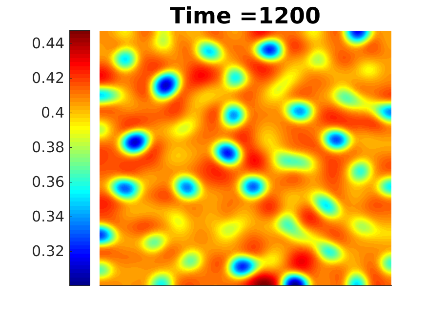
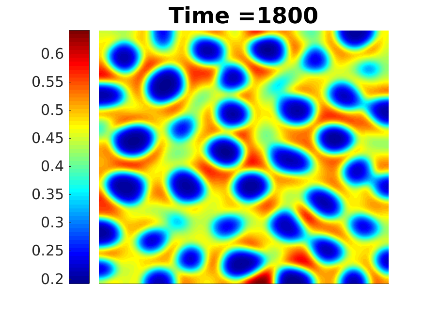
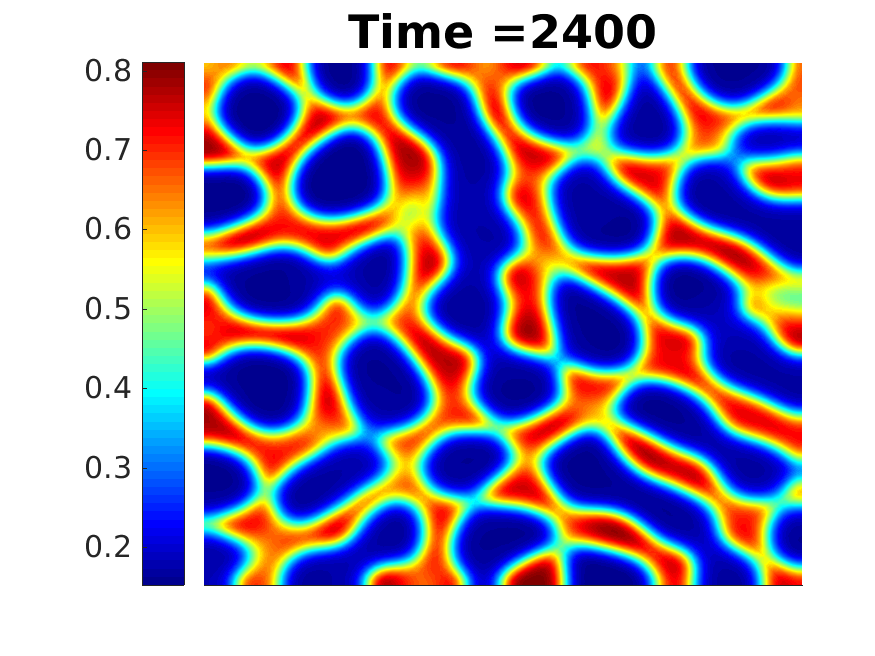
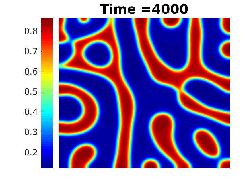
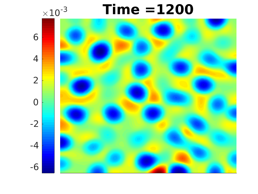
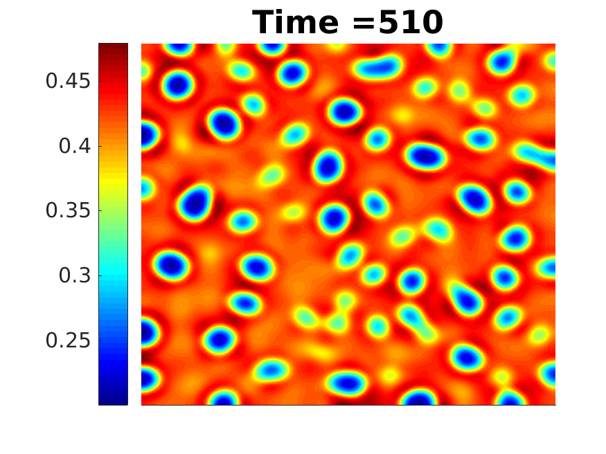
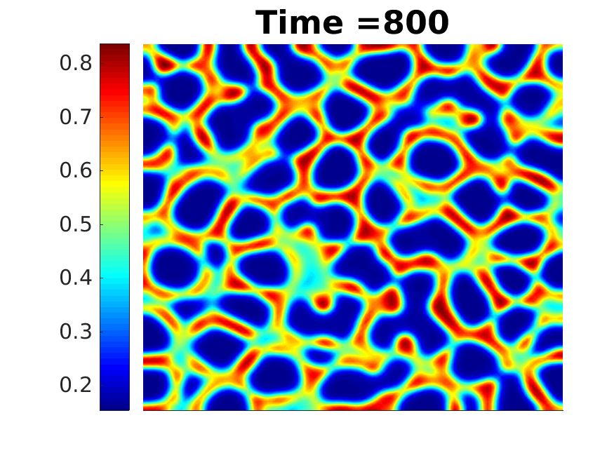
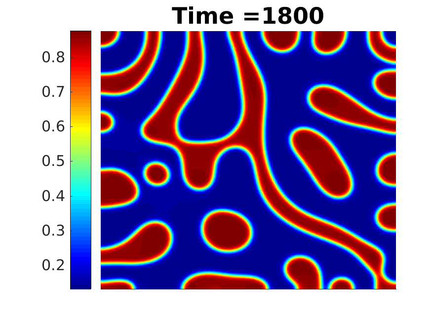
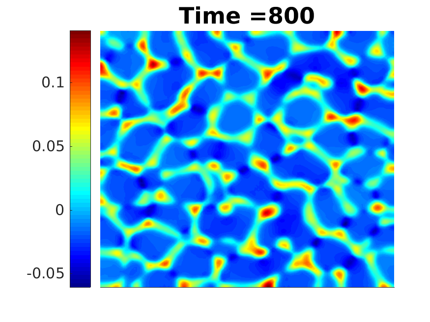
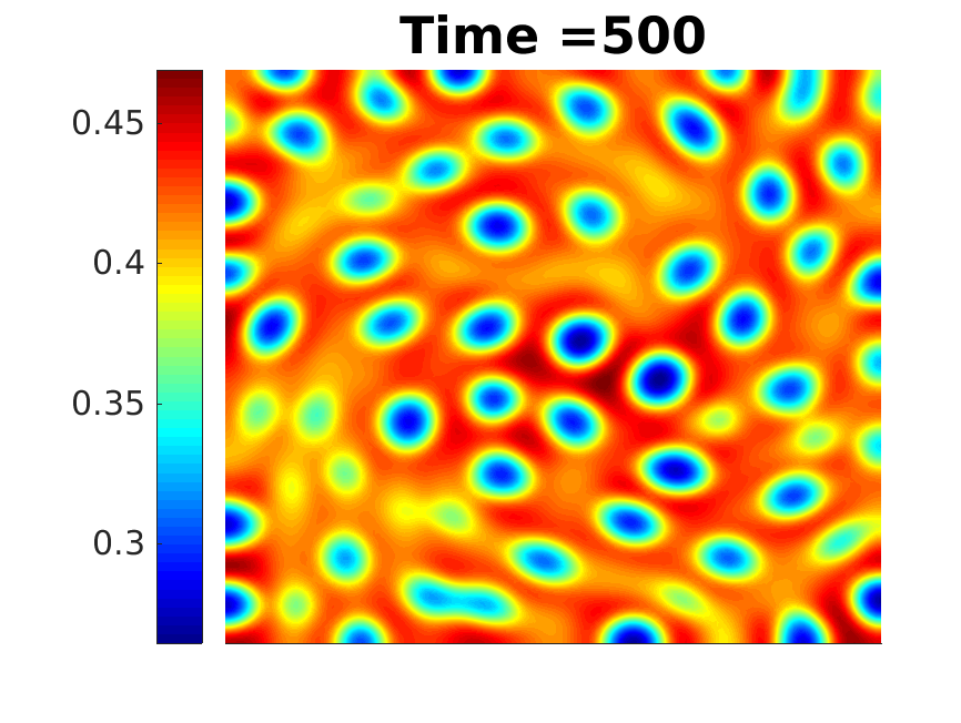
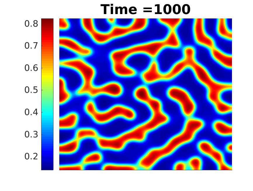
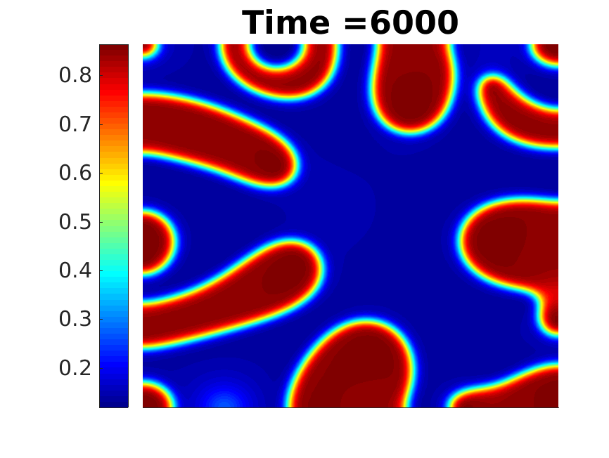
    Extensive numerical simulations, from which a representative choice is presented in Section 9, confirm a good agreement with physical experiments of dynamical asymmetric mixtures, see [51]. In particular, formation of a new phenomena, such as transient network-like polymeric structures and volume shrinking has been observed, too. Mathematically speaking, the cross-diffusion terms in the (ϕ,q)(\phi,q)-subsystem, cf. (2.6), yield a realistic model for structure formation effects, such as transient network-like polymeric structures.

  • •

    In this paper we consider a regular case with a polynomial-like potential function and suitably bounded mobilities. Based on the current results we will study in our subsequent work [12] the existence of a global weak solution for the case with logarithmic Flory-Huggins potential and degenerate mobilities with possibly different rates. We refer a reader to [22] where similar situation with one mobility function has been studied.

The paper is organized in the following way. In Section 2 we present the mathematical model for viscoelastic phase separation. The weak solution to our viscoelastic phase separation model is introduced in Section 3 and the main result on the existence of global weak solutions is formulated in Section 4. Sections 5-8 are devoted to the proof of our main result. In Section 9 we propose a Lagrange-Galerkin finite element method. Further, we present several numerical simulations of spinodal decomposition. Numerical experiments indicate that our numerical method is energy-stable and mass conservative.

2 Mathematical Model

The viscoelastic phase separation can be described by a coupled system consisting of the Cahn-Hilliard equation for phase field evolution, the Navier-Stokes equation for fluid flow and the time evolution of the viscoelastic conformation tensor. A classical approach to model the evolution of interfaces is the diffusive interface theory.
In the recent paper by Zhou et al. [55] the classical interface theory has been combined with time evolution of a viscoelastic fluid in order to model viscoelastic phase separation. The total energy of the polymer-solvent mixture consists of the mixing energy between the polymer and the solvent, the bulk stress energy, the elastic energy and the kinetic energy.

Et​o​t​(ϕ,q,𝐂,𝐮)\displaystyle E_{tot}(\phi,q,\mathbf{C},\mathbf{u}) =Em​i​x​(ϕ)+Eb​u​l​k​(q)+Ee​l​(𝐂)+Ek​i​n​(𝐮)\displaystyle=E_{mix}(\phi)+E_{bulk}(q)+E_{el}(\mathbf{C})+E_{kin}(\mathbf{u}) (2.1)
=∫Ω(c02​|∇ϕ|2+F⁡(ϕ))+∫Ω12​q2+∫Ω(14​tr​(tr⁡(𝐂)​𝐂−2​ln⁡(𝐂)−𝐈))+∫Ω12​|𝐮|2,\displaystyle=\int_{\Omega}\left(\frac{c_{0}}{2}\left|\nabla\phi\right|^{2}+F(\phi)\right)+\int_{\Omega}\frac{1}{2}q^{2}+\int_{\Omega}\left(\frac{1}{4}\mathrm{tr}\left({\mathrm{tr}(\mathbf{C})\mathbf{C}-2\ln(\mathbf{C})-\mathbf{I}}\right)\right)+\int_{\Omega}\frac{1}{2}\left|\mathbf{u}\right|^{2},

where ϕ\phi denotes the volume fraction of polymer molecules, q​𝐈q\mathbf{I} the bulk stress arising from polymeric interactions, 𝐂\mathbf{C} the viscoelastic conformation tensor and 𝐮\mathbf{u} the volume averaged velocity consisting of solvent and polymer velocity. Furthermore, c0c_{0} is a positive constant controlling the interface width. In the present work we will work with the Ginzburg-Landau potential,

F⁡(ϕ)=a​ϕ2​(ϕ−1)2,F(\phi)=a\phi^{2}(\phi-1)^{2}, (2.2)

which is typically used as a regular approximation of the (more physically relevant) logarithmic Flory-Huggins potential

Fl​o​g​(ϕ)=1np​ϕ​ln⁡(ϕ)+1ns​(1−ϕ)​ln⁡(1−ϕ)+χ​ϕ​(1−ϕ),F_{log}(\phi)=\frac{1}{n_{p}}\phi\ln(\phi)+\frac{1}{n_{s}}(1-\phi)\ln(1-\phi)+\chi\phi(1-\phi), (2.3)

where np,nsn_{p},n_{s} stand for the molecular weights of the polymer and solvent, respectively. χ\chi is the so-called Flory interaction parameter which describes the interaction between the two components and is proportional to the inverse temperature.
In the forthcoming analysis it will be enough to assume the potential behaves like a polynomial. More precisely, we assume that the potential F∈C2​(ℝ)F\in C^{2}(\mathbb{R}) and there are constants ci>0c_{i}>0 for i∈{1,…,7}i\in\{1,\ldots,7\} and c8≥0c_{8}\geq 0 that the following holds true,

|F⁡(s)|≤c1​|s|p+c2\displaystyle|F(s)|\leq c_{1}|s|^{p}+c_{2} ,|F′(s)|≤c3|s|p−1+c4,|F′′(s)|≤c5|s|p−2+c6 for p≥2,\displaystyle,\hskip 10.00002pt|F^{\prime}(s)|\leq c_{3}|s|^{p-1}+c_{4},\hskip 10.00002pt|F^{\prime\prime}(s)|\leq c_{5}|s|^{p-2}+c_{6}\textnormal{ for }p\geq 2, (2.4)
F⁡(s)≥−c7\displaystyle F(s)\geq-c_{7} ,F′′(s)≥−c8.\displaystyle,\quad F^{\prime\prime}(s)\geq-c_{8}. (2.5)

Further, we will set F′​(s)=f​(s)F^{\prime}(s)=f(s).

Following [55] we can derive a multiphase model for the viscoelastic phase separation, see also Appendix, where a brief derivation in the context of GENERIC [28, 29] and of [45, 46] is presented.

∂ϕ∂t+𝐮⋅∇ϕ=div(m(ϕ)∇μ)−κdiv(n(ϕ)∇(A(ϕ)q))∂q∂t+𝐮⋅∇q=−1τ⁡(ϕ)q+A(ϕ)Δ(A(ϕ)q)−κA(ϕ)div(n(ϕ)∇μ)∂𝐮∂t+(𝐮⋅∇)𝐮=div(η(ϕ)(∇𝐮+(∇𝐮)⊤))−∇p+div𝐓+∇ϕμ∂𝐂∂t+(𝐮⋅∇)𝐂=(∇𝐮)​𝐂+𝐂​(∇𝐮)⊤+χ⁡(ϕ,tr⁡(𝐂))​𝐈−Φ⁡(ϕ,tr⁡(𝐂))​𝐂+ε​Δ​𝐂div⁡(𝐮)=0𝐓=tr⁡(𝐂)​𝐂μ=−c0​Δ​ϕ+f⁡(ϕ)\displaystyle\begin{split}\frac{\partial\phi}{\partial t}+\hskip 10.00002pt\mathbf{u}\cdot\nabla\phi&=\mathrm{div}\big({m(\phi)\nabla\mu}\big)-\kappa\mathrm{div}\big({n(\phi)\nabla\big(A(\phi)q\big)}\big)\\ \frac{\partial q}{\partial t}+\hskip 10.00002pt\mathbf{u}\cdot\nabla q&=-\frac{1}{\tau(\phi)}q+A(\phi)\Delta\big(A(\phi)q\big)-\kappa A(\phi)\mathrm{div}\big({n(\phi)\nabla\mu}\big)\\ \frac{\partial\mathbf{u}}{\partial t}+(\mathbf{u}\cdot\nabla)\mathbf{u}&=\mathrm{div}\big({\eta(\phi)\big(\nabla\mathbf{u}+(\nabla\mathbf{u})^{\top}\big)}\big)-\nabla p+\mathrm{div}\,{\mathbf{T}}+\nabla\phi\mu\\ \frac{\partial\mathbf{C}}{\partial t}+(\mathbf{u}\cdot\nabla)\mathbf{C}&=(\nabla\mathbf{u})\mathbf{C}+\mathbf{C}(\nabla\mathbf{u})^{\top}+\mbox{\large$\chi$}(\phi,\mathrm{tr}(\mathbf{C}))\mathbf{I}-\Phi(\phi,\mathrm{tr}(\mathbf{C}))\mathbf{C}+\varepsilon\Delta\mathbf{C}\\ \mathrm{div}\left({\mathbf{u}}\right)&=0\hskip 28.45274pt\mathbf{T}=\mathrm{tr}\left({\mathbf{C}}\right)\mathbf{C}\hskip 28.45274pt\mu=-c_{0}\Delta\phi+f(\phi)\end{split} (2.6)

Here we have denoted by μ\mu the chemical potential. This allows us to write (2.6) in the saddle point form which is more convenient for our further study. System (2.6) is formulated on (0,T)×Ω(0,T)\times\Omega, where Ω⊂ℝ2\Omega\subset\mathbb{R}^{2} is a bounded domain with a Lipschitz-continuous boundary. Our model is equipped with the following initial and boundary conditions

(ϕ,q,𝐮,𝐂)|t=0=(ϕ0,q0,𝐮0,𝐂0),∂nϕ|∂Ω=∂nμ|∂Ω=∂nq|∂Ω=0,𝐮|∂Ω=𝟎,∂n𝐂|∂Ω=𝟎.\displaystyle\left.(\phi,q,\mathbf{u},\mathbf{C})\right|_{t=0}=(\phi_{0},q_{0},\mathbf{u}_{0},\mathbf{C}_{0}),\quad\left.\partial_{n}\phi\right|_{\partial\Omega}=\left.\partial_{n}\mu\right|_{\partial\Omega}=\left.\partial_{n}q\right|_{\partial\Omega}=0,\quad\left.\mathbf{u}\right|_{\partial\Omega}=\mathbf{0},\quad\left.\partial_{n}\mathbf{C}\right|_{\partial\Omega}=\mathbf{0}.

The viscoelastic stress tensor is given by

𝐓=tr⁡(𝐂)​𝐂.\mathbf{T}=\mathrm{tr}\left({\mathbf{C}}\right)\mathbf{C}.

The functions m⁡(ϕ),n⁡(ϕ)m(\phi),n(\phi) stand for mobility functions, τ⁡(ϕ),χ​(ϕ,tr⁡(𝐂))−1,Φ​(ϕ,tr⁡(𝐂))−1\tau(\phi),\mbox{\large$\chi$}(\phi,\mathrm{tr}\left({\mathbf{C})}\right)^{-1},\Phi(\phi,\mathrm{tr}\left({\mathbf{C}}\right))^{-1} describe generalized relaxation times, A⁡(ϕ)A(\phi) the bulk modulus, η⁡(ϕ)\eta(\phi) the viscosity, ε\varepsilon the viscoelastic diffusion parameter and κ\kappa a positive constant. These functions will be specified in Section 2.1.

2.1 Assumptions

In what follows, we will assume that all of the coefficient functions are continuous, positive and bounded, i.e.

0<τ1≤τ⁡(s)≤τ2,0<A1≤A⁡(s)≤A2,0<η1≤η⁡(s)≤η2​ for all ​s∈ℝ.0<\tau_{1}\leq\tau(s)\leq\tau_{2},\hskip 10.00002pt0<A_{1}\leq A(s)\leq A_{2},\hskip 10.00002pt0<\eta_{1}\leq\eta(s)\leq\eta_{2}\textrm{ for all }s\in\mathbb{R}. (2.7)

Additionally A⁡(s)A(s) is a C1−C^{1}-function and ‖A′‖∞≤A2′.\left\|A^{\prime}\right\|_{\infty}\leq A_{2}^{\prime}. For the generalized relaxation times χ\chi and Φ\Phi we choose analogously as in [38]

χ⁡(ϕ,𝐂)=h⁡(ϕ)​tr​(𝐂),Φ⁡(ϕ,𝐂)=h⁡(ϕ)​tr​(𝐂)2.\mbox{\large$\chi$}(\phi,\mathbf{C})=h(\phi)\mathrm{tr}\left({\mathbf{C}}\right),\hskip 20.00003pt\Phi(\phi,\mathbf{C})=h(\phi)\mathrm{tr}\left({\mathbf{C}}\right)^{2}. (2.8)

Let us point out that it may be possible to generalize our results similarly as in [37] for

χ⁡(ϕ,𝐂)=h⁡(ϕ)​tr​(𝐂)α−1,Φ⁡(ϕ,𝐂)=h⁡(ϕ)​tr​(𝐂)α,α∈[1,6].\mbox{\large$\chi$}(\phi,\mathbf{C})=h(\phi)\mathrm{tr}\left({\mathbf{C}}\right)^{\alpha-1},\hskip 20.00003pt\Phi(\phi,\mathbf{C})=h(\phi)\mathrm{tr}\left({\mathbf{C}}\right)^{\alpha},\;\alpha\in[1,6].

We further assume that the functions h,m,nh,m,n are continuous, positive and bounded,

0<h1≤h⁡(s)≤h2,  0≤m1≤m⁡(s)≤m2​ and ​0≤n1<n⁡(s)≤n2​ for all ​s∈ℝ.0<h_{1}\leq h(s)\leq h_{2},\;\;0\leq m_{1}\leq m(s)\leq m_{2}\textrm{ and }0\leq n_{1}<n(s)\leq n_{2}\textrm{ for all }s\in\mathbb{R}. (2.9)

The case m1,n1>0m_{1},n_{1}>0 is called regular case. In our future work [12] we extend the present study to the so-called degenerate case, where m1=n1=0.m_{1}=n_{1}=0.

2.2 Preliminaries

In this section we introduce suitable notation and required analytical tools. For the standard Lebesgue spaces Lp​(Ω)L^{p}(\Omega) the norm is denoted by ‖⋅‖p\left\|\cdot\right\|_{p}. Further, we denote the space of divergence free and mean free functions by the

Ldiv2(Ω):=C0,div∞​(Ω)¯‖⋅‖2,L02(Ω):={u∈L2(Ω)|∫Ωudx=0},L^{2}_{\text{div}}(\Omega):=\overline{C_{0,\text{div}}^{\infty}(\Omega)}^{\left\|\cdot\right\|_{2}},\hskip 20.00003ptL^{2}_{0}(\Omega):=\left\{u\in L^{2}(\Omega)\mathrel{\bigg|}\int_{\Omega}u\,\mathrm{d}x=0\right\},

respectively. We use the standard notation for the Sobolev spaces and set

V:=H0,div1​(Ω)2,H:=Ldiv2​(Ω)2,W:=H1​(Ω)2×2.V:=H^{1}_{0,\text{div}}(\Omega)^{2},\hskip 20.00003ptH:=L^{2}_{\text{div}}(\Omega)^{2},\hskip 20.00003ptW:=H^{1}(\Omega)^{2\times 2}.

The space VV is equipped with the norm ‖⋅‖V:=‖∇⋅‖2\left\|\cdot\right\|_{V}:=\left\|\nabla\cdot\right\|_{2}. We denote the norms of the corresponding Bochner space Lp​(0,T,Lq​(Ω))L^{p}(0,T;L^{q}(\Omega)) by ‖⋅‖Lp​(Lq).\left\|\cdot\right\|_{L^{p}(L^{q})}.

In what follows, we state several inequalities that will be used later.

Proposition 2.1 ([7],[34]).

Let Ω⊂ℝ2\Omega\subset\mathbb{R}^{2} be a bounded smooth domain. Then the following inequalities hold true

‖u‖4\displaystyle\left\|u\right\|_{4} ≤c​‖u‖21/2​‖∇u‖21/2,u∈H01​(Ω)\displaystyle\leq c\left\|u\right\|_{2}^{1/2}\left\|\nabla u\right\|_{2}^{1/2},\hskip 77.00008ptu\in H^{1}_{0}(\Omega) (2.10)
‖v‖4\displaystyle\left\|v\right\|_{4} ≤c⁡(Ω)​(‖v‖+‖v‖21/2​‖∇v‖21/2),v∈H1​(Ω)\displaystyle\leq c(\Omega)\left(\|v\|+\left\|v\right\|_{2}^{1/2}\left\|\nabla v\right\|_{2}^{1/2}\right),\hskip 21.00009ptv\in H^{1}(\Omega) (2.11)
‖u‖r\displaystyle\left\|u\right\|_{r} ≤c⁡(Ω)​(‖v‖2+‖v‖22/r​‖∇u‖2(r−2)/r), for ​r>2,v∈H1​(Ω)\displaystyle\leq c(\Omega)\left(\left\|v\right\|_{2}+\left\|v\right\|_{2}^{2/r}\left\|\nabla u\right\|_{2}^{(r-2)/r}\right),\text{ for }r>2,v\in H^{1}(\Omega) (2.12)
‖v‖∞\displaystyle\left\|v\right\|_{\infty} ≤c​‖v‖21/2​‖v‖2,21/2,v∈H2​(Ω)∩H01​(Ω).\displaystyle\leq c\left\|v\right\|_{2}^{1/2}\left\|v\right\|_{2,2}^{1/2},\hskip 85.00012ptv\in H^{2}(\Omega)\cap H^{1}_{0}(\Omega). (2.13)
Lemma 2.2.

Suppose that there are two sequences {un},{vn}\{u_{n}\},\{v_{n}\} and a bounded domain DD with the following properties

  1. 1.

    un→uu_{n}\rightarrow u a.e in DD and ‖un‖∞≤c<∞\left\|u_{n}\right\|_{\infty}\leq c<\infty for all nn

  2. 2.

    vn⇀vv_{n}\rightharpoonup v in L2​(D)L^{2}(D).

Then the product un​vnu_{n}v_{n} converges weakly to u​vuv in L2​(D)L^{2}(D).

Proof.

Weak convergence of un​vnu_{n}v_{n} in L2​(D)L^{2}(D) is defined by

∫D(un​vn−u​v)​g⟶0,n→∞​ for all ​g∈L2​(D).\int_{D}\big(u_{n}v_{n}-uv\big)g\longrightarrow 0,n\rightarrow\infty\;\text{ for all }g\in L^{2}(D). (2.14)

Splitting the integral we obtain

|∫D(un​vn−u​v)​g|≤|∫Dg​vn​(un−u)|+|∫Dg​u​(vn−v)|\left|\int_{D}\big(u_{n}v_{n}-uv\big)g\right|\leq\left|\int_{D}gv_{n}\big(u_{n}-u\big)\right|+\left|\int_{D}gu\big(v_{n}-v\big)\right| (2.15)

The first integral can be controlled by ‖g​un−g​u‖2​‖vn‖2\left\|gu_{n}-gu\right\|_{2}\left\|v_{n}\right\|_{2} which goes to zero due to the boundedness of vnv_{n} in L2​(D)L^{2}(D) and the strong convergence of g​ungu_{n} in L2​(D)L^{2}(D). This strong convergence can be achieved by the generalized dominated convergence theorem. Since g​u∈L2​(D)gu\in L^{2}(D), the second integral tends to zero due to the weak convergence of vnv_{n}. Note that in the proof we have also shown that g​ungu_{n} converges strongly in L2​(D)L^{2}(D). ∎

We will frequently use the interpolation spaces and their norms.

Lemma 2.3 ([9]).

Let X⊂Y⊂ZX\subset Y\subset Z three Hilbert spaces, and suppose that the embedding of XX in YY is compact. Then:

  1. i)

    For any p,q∈(1,∞)p,q\in(1,\infty) the embedding

    {f∈Lp​(0,T,X),d​fd​t∈Lq​(0,T,Z)}↪Lp​(0,T,Y)\left\{f\in L^{p}(0,T;X),\frac{\,\mathrm{d}f}{\,\mathrm{d}t}\in L^{q}(0,T;Z)\right\}\hookrightarrow L^{p}(0,T;Y)

    is compact.

  2. ii)

    For any p>1p>1 the embedding

    {f∈L∞​(0,T,X),d​fd​t∈Lp​(0,T,Z)}↪C⁡([0,T],Y)\left\{f\in L^{\infty}(0,T;X),\frac{\,\mathrm{d}f}{\,\mathrm{d}t}\in L^{p}(0,T;Z)\right\}\hookrightarrow C([0,T];Y)

    is compact.

  3. iii)

    The following continuous embeddings holds

    {f∈L2​(0,T,X),d​fd​t∈L2​(0,T,Y)}↪C⁡(0,T,[X,Y]12).\left\{f\in L^{2}(0,T;X),\frac{\,\mathrm{d}f}{\,\mathrm{d}t}\in L^{2}(0,T;Y)\right\}\hookrightarrow C(0,T;[X,Y]_{\frac{1}{2}}).

The space [X,Y]12[X,Y]_{\frac{1}{2}} is an interpolation space, see [9], and we will use this result for the spaces [H2,H−1]12=H1/2[H^{2},H^{-1}]_{\frac{1}{2}}=H^{1/2}.

Proposition 2.4.

For a matrix valued function 𝐃∈ℝd×d\mathbf{D}\in\mathbb{R}^{d\times d} and p≥2p\geq 2 we have

‖tr⁡(𝐃)‖pp:=∫Ω(∑i=1d𝐃i​i)p​𝑑x≤dp−1​∫Ω∑i,j=1d|𝐃i​jp|​𝑑x=:‖𝐃‖pp.\left\|\mathrm{tr}\left({\mathbf{D}}\right)\right\|^{p}_{p}:=\int_{\Omega}\left(\sum_{i=1}^{d}\mathbf{D}_{ii}\right)^{p}\,\mathrm{d}x\leq d^{p-1}\int_{\Omega}\sum_{i,j=1}^{d}\left|\mathbf{D}_{ij}^{p}\right|\,\mathrm{d}x=:\left\|\mathbf{D}\right\|^{p}_{p}.

For symmetric positive definite matrices both norms are equivalent.

The norm ‖𝐃‖p\left\|\mathbf{D}\right\|_{p} is the so-called Frobenius norm. We denote by 𝐂:𝐃=tr⁡(𝐂𝐃⊤)\mathbf{C}:\mathbf{D}=\mathrm{tr}\left({\mathbf{C}\mathbf{D}^{\top}}\right) the Frobenius inner product.

Proposition 2.5 ([53], [38]).

For any open set Ω⊂ℝ2\Omega\subset\mathbb{R}^{2} it holds that the forms

𝐛(𝐮,𝐯,𝐰)≡∫Ω(𝐮⋅∇)𝐯⋅𝐰dx and 𝐁(𝐮,𝐂,𝐃)≡∫Ω(𝐮⋅∇)𝐂:𝐃dx\mathbf{b}(\mathbf{u},\mathbf{v},\mathbf{w})\equiv\int_{\Omega}(\mathbf{u}\cdot\nabla)\mathbf{v}\cdot\mathbf{w}\,\mathrm{d}x\text{ and }\;\;\mathbf{B}(\mathbf{u},\mathbf{C},\mathbf{D})\equiv\int_{\Omega}(\mathbf{u}\cdot\nabla)\mathbf{C}:\mathbf{D}\,\mathrm{d}x

are continuous and trilinear on V×V×VV\times V\times V and V×W×WV\times W\times W, respectively. Further the following properties hold

𝐛⁡(𝐮,𝐮,𝐯)\displaystyle\mathbf{b}(\mathbf{u},\mathbf{u},\mathbf{v}) =−𝐛⁡(𝐮,𝐯,𝐮),𝐮∈V,𝐯∈H01\displaystyle=-\mathbf{b}(\mathbf{u},\mathbf{v},\mathbf{u}),\;\;\;\;\;\;\;\;\;\;\mathbf{u}\in V,\mathbf{v}\in H^{1}_{0}
𝐁⁡(𝐮,𝐂,𝐃)\displaystyle\mathbf{B}(\mathbf{u},\mathbf{C},\mathbf{D}) =−𝐁(𝐮,𝐃,𝐂),𝐮∈V,𝐂,𝐃∈W\displaystyle=-\mathbf{B}(\mathbf{u},\mathbf{D},\mathbf{C}),\;\;\;\;\;\;\;\mathbf{u}\in V,\mathbf{C},\mathbf{D}\in W
|𝐛⁡(𝐮,𝐰,𝐯)|\displaystyle\left|\mathbf{b}(\mathbf{u},\mathbf{w},\mathbf{v})\right| =|𝐛⁡(𝐮,𝐯,𝐰)|≤c​‖𝐮‖4​‖𝐯‖V​‖𝐰‖4\displaystyle=\left|\mathbf{b}(\mathbf{u},\mathbf{v},\mathbf{w})\right|\;\;\leq c\left\|\mathbf{u}\right\|_{4}\left\|\mathbf{v}\right\|_{V}\left\|\mathbf{w}\right\|_{4}
|𝐁⁡(𝐮,𝐂,𝐃)|\displaystyle\left|\mathbf{B}(\mathbf{u},\mathbf{C},\mathbf{D})\right| =|𝐁⁡(𝐮,𝐃,𝐂)|≤c​‖𝐮‖4​‖∇𝐃‖2​‖𝐂‖4.\displaystyle=\left|\mathbf{B}(\mathbf{u},\mathbf{D},\mathbf{C})\right|\leq c\left\|\mathbf{u}\right\|_{4}\left\|\nabla\mathbf{D}\right\|_{2}\left\|\mathbf{C}\right\|_{4}.
Lemma 2.6 (Korn inequality, [33]).

Let Ω\Omega be an open and regular set of ℝ2\mathbb{R}^{2} and 𝐮∈H01​(Ω)\mathbf{u}\in H^{1}_{0}(\Omega) a vector field on Ω\Omega, then we have

‖∇𝐮‖2≤2​‖D​𝐮‖2,\left\|\nabla\mathbf{u}\right\|_{2}\leq\sqrt{2}\left\|\mathrm{D}\mathbf{u}\right\|_{2},

with the equality if div⁡(𝐮)=0\mathrm{div}\left({\mathbf{u}}\right)=0. Suppose η\eta is a continuous function satisfying (2.7) then the inequality

‖η∇𝐮‖2≤2‖ηD𝐮‖2\left\|\sqrt{\eta}\nabla\mathbf{u}\right\|_{2}\leq\sqrt{2}\left\|\sqrt{\eta}\mathrm{D}\mathbf{u}\right\|_{2}

holds. Here D​𝐮\mathrm{D}\mathbf{u} denotes the deformation tensor which is the symmetric part of ∇𝐮\nabla\mathbf{u}, i.e.

D​𝐮=12​(∇𝐮+∇𝐮T).\mathrm{D}\mathbf{u}=\frac{1}{2}\left(\nabla\mathbf{u}+\nabla\mathbf{u}^{T}\right).

For the limiting process we will need the following lemma which is a consequence of the Vitali theorem.

Lemma 2.7 (Vitali theorem [24]).

Let M⊂ℝdM\subset\mathbb{R}^{d} be a measurable and bounded set. Let the sequence {fm}m∈ℕ\{f_{m}\}_{m\in\mathbb{N}} be uniformly bounded in Lq​(M)L^{q}(M) for q>1q>1. Finally, let fm→ff_{m}\to f a.e. in MM for some f∈Lq​(M)f\in L^{q}(M). Then

∫Mfm→∫Mf.\int_{M}f_{m}\to\int_{M}f.
Lemma 2.8 ([9]).

If ϕ∈Hs+2​(Ω)\phi\in H^{s+2}(\Omega), then ‖ϕ−(ϕ)Ω‖Hs+2≤C​‖Δ​ϕ‖Hs\|\phi-(\phi)_{\Omega}\|_{H^{s+2}}\leq C\|\Delta\phi\|_{H^{s}}. Here (ϕ)Ω:=1|Ω|​∫Ωϕ​𝑑x(\phi)_{\Omega}:=\frac{1}{\left|\Omega\right|}\int_{\Omega}\phi\,\mathrm{d}x denotes the mean value.

Lemma 2.9 ([8]).

Let 𝐃∈H2​(Ω)m×m∩C1​(Ω¯)m×m,m∈ℕ\mathbf{D}\in H^{2}(\Omega)^{m\times m}\cap C^{1}(\overline{\Omega})^{m\times m},m\in\mathbb{N}, be a symmetric matrix function, which is uniformly positive definite on Ω¯\overline{\Omega} and satisfies homogeneous Neumann boundary conditions, then

∫ΩΔ𝐃:𝐃−1dx=−∫Ω∇𝐃:∇𝐃−1dx≥1m∫Ω|∇tr(log(𝐃))|2dx\int_{\Omega}\Delta\mathbf{D}:\mathbf{D}^{-1}\,\mathrm{d}x=-\int_{\Omega}\nabla\mathbf{D}:\nabla\mathbf{D}^{-1}\,\mathrm{d}x\geq\frac{1}{m}\int_{\Omega}\left|\nabla\mathrm{tr}\left({\log(\mathbf{D})}\right)\right|^{2}\,\mathrm{d}x (2.16)

3 Weak solution

In this section we will introduce the weak solutions to our viscoelastic phase separation model (2.6) and derive the corresponding energy estimates.

Definition 3.1.

Let the initial data (ϕ0,q0,𝐮0,𝐂0)∈H1​(Ω)×L2​(Ω)×H×L2​(Ω)2×2\left(\phi_{0},q_{0},\mathbf{u}_{0},\mathbf{C}_{0}\right)\in H^{1}(\Omega)\times L^{2}(\Omega)\times H\times L^{2}(\Omega)^{2\times 2}. The quintuple (ϕ,q,μ,𝐮,𝐂)(\phi,q,\mu,\mathbf{u},\mathbf{C}) is called a corresponding weak solution of (2.6), if

ϕ∈L∞​(0,T,H1​(Ω))∩L2​(0,T,H2​(Ω)),\displaystyle\phi\in L^{\infty}(0,T;H^{1}(\Omega))\cap L^{2}(0,T;H^{2}(\Omega)), q∈L∞​(0,T,L2​(Ω))∩L2​(0,T,H1​(Ω)),\displaystyle q\in L^{\infty}(0,T;L^{2}(\Omega))\cap L^{2}(0,T;H^{1}(\Omega)), μ∈L2​(0,T,H1​(Ω)),\displaystyle\mu\in L^{2}(0,T;H^{1}(\Omega)),
𝐮∈L∞​(0,T,L2​(Ω))∩L2​(0,T,V),\displaystyle\mathbf{u}\in L^{\infty}(0,T;L^{2}(\Omega))\cap L^{2}(0,T;V), 𝐂∈L∞​(0,T,L2​(Ω))∩L2​(0,T,W),\displaystyle\mathbf{C}\in L^{\infty}(0,T;L^{2}(\Omega))\cap L^{2}(0,T;W),
∂ϕ∂t∈L2​(0,T,H−1​(Ω)),\displaystyle\frac{\partial\phi}{\partial t}\in L^{2}(0,T;H^{-1}(\Omega)), ∂q∂t∈L4/3​(0,T,H−1​(Ω)),\displaystyle\frac{\partial q}{\partial t}\in L^{4/3}(0,T;H^{-1}(\Omega)), ∂𝐮∂t∈L2​(0,T,V⋆),\displaystyle\frac{\partial\mathbf{u}}{\partial t}\in L^{2}(0,T;V^{\star}), ∂𝐂∂t∈L4/3​(0,T,W⋆),\displaystyle\frac{\partial\mathbf{C}}{\partial t}\in L^{4/3}(0,T;W^{\star}),

and

∫Ω∂ϕ∂tψdx+∫Ω𝐮⋅∇ϕψdx+∫Ωm(ϕ)∇μ∇ψdx−κ∫Ωn(ϕ)∇(A(ϕ)q)∇ψdx\displaystyle\int_{\Omega}\frac{\partial\phi}{\partial t}\psi\,\mathrm{d}x+\int_{\Omega}\mathbf{u}\cdot\nabla\phi\psi\,\mathrm{d}x+\int_{\Omega}m(\phi)\nabla\mu\nabla\psi\,\mathrm{d}x-\kappa\int_{\Omega}n(\phi)\nabla(A(\phi)q)\nabla\psi\,\mathrm{d}x =0\displaystyle=0
∫Ω∂q∂tζdx+∫Ω𝐮⋅∇qζdx+∫Ωq​ζτ⁡(ϕ)dx+∫Ω∇(A(ϕ)q)∇(A(ϕ)ζ)dx−κ∫Ωn(ϕ)∇μ∇(A(ϕ)ζ)dx\displaystyle\int_{\Omega}\frac{\partial q}{\partial t}\zeta\,\mathrm{d}x+\int_{\Omega}\mathbf{u}\cdot\nabla q\zeta\,\mathrm{d}x+\int_{\Omega}\frac{q\zeta}{\tau(\phi)}\,\mathrm{d}x+\int_{\Omega}\nabla(A(\phi)q)\nabla(A(\phi)\zeta)\,\mathrm{d}x-\kappa\int_{\Omega}n(\phi)\nabla\mu\nabla(A(\phi)\zeta)\,\mathrm{d}x =0\displaystyle=0
∫Ωμξdx−c0∫Ω∇ϕ∇ξdx−∫Ωf(ϕ)ξdx\displaystyle\int_{\Omega}\mu\xi\,\mathrm{d}x-c_{0}\int_{\Omega}\nabla\phi\nabla\xi\,\mathrm{d}x-\int_{\Omega}f(\phi)\xi\,\mathrm{d}x =0\displaystyle=0
∫Ω∂𝐮∂t⋅𝐯dx+∫Ω(𝐮⋅∇)𝐮⋅𝐯dx−∫Ωη(ϕ)D𝐮:D𝐯dx+∫Ω𝐓:∇𝐯dx+∫Ωϕ∇μ⋅𝐯dx\displaystyle\int_{\Omega}\frac{\partial\mathbf{u}}{\partial t}\cdot\mathbf{v}\,\mathrm{d}x+\int_{\Omega}(\mathbf{u}\cdot\nabla)\mathbf{u}\cdot\mathbf{v}\,\mathrm{d}x-\int_{\Omega}\eta(\phi)\mathrm{D}\mathbf{u}:\mathrm{D}\mathbf{v}\,\mathrm{d}x+\int_{\Omega}\mathbf{T}:\nabla\mathbf{v}\,\mathrm{d}x+\int_{\Omega}\phi\nabla\mu\cdot\mathbf{v}\,\mathrm{d}x =0\displaystyle=0
∫Ω∂𝐂∂t:𝐃dx+∫Ω(𝐮⋅∇)𝐂:𝐃dx−∫Ω[(∇𝐮)𝐂+𝐂(∇𝐮)T]:𝐃dx+ε∫Ω∇𝐂:∇𝐃dx\displaystyle\int_{\Omega}\frac{\partial\mathbf{C}}{\partial t}:\mathbf{D}\,\mathrm{d}x+\int_{\Omega}(\mathbf{u}\cdot\nabla)\mathbf{C}:\mathbf{D}\,\mathrm{d}x-\int_{\Omega}\left[(\nabla\mathbf{u})\mathbf{C}+\mathbf{C}(\nabla\mathbf{u})^{T}\right]:\mathbf{D}\,\mathrm{d}x+\varepsilon\int_{\Omega}\nabla\mathbf{C}:\nabla\mathbf{D}\,\mathrm{d}x
=−∫Ωh(ϕ)tr(𝐂)2𝐂:𝐃dx+∫Ωh(ϕ)tr(𝐂)𝐈:𝐃dx,\displaystyle=-\int_{\Omega}h(\phi)\mathrm{tr}\left({\mathbf{C}}\right)^{2}\mathbf{C}:\mathbf{D}\,\mathrm{d}x+\int_{\Omega}h(\phi)\mathrm{tr}\left({\mathbf{C}}\right)\mathbf{I}:\mathbf{D}\,\mathrm{d}x, (3.1)

for any test function (ψ,ζ,ξ,𝐯,𝐃)∈H1​(Ω)3×V×W(\psi,\zeta,\xi,\mathbf{v},\mathbf{D})\in H^{1}(\Omega)^{3}\times V\times W and almost every t∈(0,T).t\in(0,T). For the initial data it holds that (ϕ⁡(0),q⁡(0),𝐮⁡(0),𝐂⁡(0))=(ϕ0,q0,𝐮0,𝐂0)\left(\phi(0),q(0),\mathbf{u}(0),\mathbf{C}(0)\right)=\left(\phi_{0},q_{0},\mathbf{u}_{0},\mathbf{C}_{0}\right).

Theorem 3.2.

Let (ϕ,q,μ,𝐮,p,𝐂)(\phi,q,\mu,\mathbf{u},p,\mathbf{C}) be a smooth solution of (2.6) and let the initial datum 𝐂0\mathbf{C}_{0} be a symmetric positive definite matrix. Further assume that 𝐂\mathbf{C} is uniformly positive definite. Then the free energy given by (2.1) satisfies

ddtE(ϕ,q,𝐮,𝐂)+∫Ωη(ϕ)|D𝐮|2dx+(1−κ)∫Ωm(ϕ)|∇μ|2+(1−κ)∫Ω|∇(A(ϕ)q))|2dx+∫Ωq2τ⁡(ϕ)dx\displaystyle\frac{\mathrm{d}}{\mathrm{dt}}E(\phi,q,\mathbf{u},\mathbf{C})+\int_{\Omega}\eta(\phi)\left|\mathrm{D}\mathbf{u}\right|^{2}\,\mathrm{d}x+(1-\kappa)\int_{\Omega}m(\phi)|\nabla\mu|^{2}+(1-\kappa)\int_{\Omega}|\nabla(A(\phi)q))|^{2}\,\mathrm{d}x+\int_{\Omega}\frac{q^{2}}{\tau(\phi)}\,\mathrm{d}x
+ε2∫Ω|∇tr(𝐂)|2dx+12∫Ωtr(𝐓)tr(𝐓+𝐓−1−2𝐈)dx+ε4∫Ω|∇tr(ln(𝐂))|2dx≤0,\displaystyle\hskip 17.07182pt+\frac{\varepsilon}{2}\int_{\Omega}\left|\nabla\mathrm{tr}\left({\mathbf{C}}\right)\right|^{2}\,\mathrm{d}x+\frac{1}{2}\int_{\Omega}\mathrm{tr}\left({\mathbf{T}}\right)\mathrm{tr}\left({\mathbf{T}+\mathbf{T}^{-1}-2\mathbf{I}}\right)\,\mathrm{d}x+\frac{\varepsilon}{4}\int_{\Omega}\left|\nabla\mathrm{tr}\left({\ln(\mathbf{C})}\right)\right|^{2}\,\mathrm{d}x\leq 0,

thus the energy is non-increasing in time.

Proof.

We will differentiate every term of (2.6) with respect to time and show the energy dissipation

ddt∫Ωc02|∇ϕ|2+F(ϕ)dx=∫Ωc0∂∇ϕ∂t⋅∇ϕ+F′(ϕ)∂ϕ∂tdx=∫Ω−c0∂ϕ∂tΔϕ+f(ϕ)∂ϕ∂tdx=∫Ω∂ϕ∂tμdx\displaystyle\frac{\mathrm{d}}{\mathrm{dt}}\int_{\Omega}\frac{c_{0}}{2}\left|\nabla\phi\right|^{2}+F(\phi)\,\mathrm{d}x=\int_{\Omega}c_{0}\frac{\partial\nabla\phi}{\partial t}\cdot\nabla\phi+F^{\prime}(\phi)\frac{\partial\phi}{\partial t}\,\mathrm{d}x=\int_{\Omega}-c_{0}\frac{\partial\phi}{\partial t}\Delta\phi+f(\phi)\frac{\partial\phi}{\partial t}\,\mathrm{d}x=\int_{\Omega}\frac{\partial\phi}{\partial t}\mu\,\mathrm{d}x
=−∫Ω𝐮⋅∇ϕμdx+∫Ωdiv(m(ϕ)∇μ)μdx−κ∫Ωdiv(n(ϕ)∇(A(ϕ)q))μdx,\displaystyle=-\int_{\Omega}\mathbf{u}\cdot\nabla\phi\mu\,\mathrm{d}x+\int_{\Omega}\mathrm{div}\big({m(\phi)\nabla\mu}\big)\mu\,\mathrm{d}x-\kappa\int_{\Omega}\mathrm{div}\big({n(\phi)\nabla(A(\phi)q)}\big)\mu\,\mathrm{d}x,
=−∫Ω𝐮⋅∇ϕμdx−∫Ωm(ϕ)|∇μ|2dx+κ∫Ωn(ϕ)∇(A(ϕ)q)∇μdx,\displaystyle=-\int_{\Omega}\mathbf{u}\cdot\nabla\phi\mu\,\mathrm{d}x-\int_{\Omega}m(\phi)\left|\nabla\mu\right|^{2}\,\mathrm{d}x+\kappa\int_{\Omega}n(\phi)\nabla(A(\phi)q)\nabla\mu\,\mathrm{d}x,
ddt​∫Ω12​|q|2​𝑑x=∫Ω∂q∂t​q​𝑑x\displaystyle\frac{\mathrm{d}}{\mathrm{dt}}\int_{\Omega}\frac{1}{2}\left|q\right|^{2}\,\mathrm{d}x=\int_{\Omega}\frac{\partial q}{\partial t}q\,\mathrm{d}x
=−∫Ω1τ⁡(ϕ)q2dx+∫Ωdiv(∇(A(ϕ)q))A(ϕ)qdx−κ∫Ωdiv(n(ϕ)∇μ)A(ϕ)qdx\displaystyle=-\int_{\Omega}\frac{1}{\tau(\phi)}q^{2}\,\mathrm{d}x+\int_{\Omega}\mathrm{div}\big({\nabla(A(\phi)q)}\big)A(\phi)q\,\mathrm{d}x-\kappa\int_{\Omega}\mathrm{div}\big({n(\phi)\nabla\mu}\big)A(\phi)q\,\mathrm{d}x
=−∫Ω1τ⁡(ϕ)q2dx−∫Ω|∇(A(ϕ)q)|2dx+κ∫Ωn(ϕ)∇μ∇(A(ϕ)q)dx,\displaystyle=-\int_{\Omega}\frac{1}{\tau(\phi)}q^{2}\,\mathrm{d}x-\int_{\Omega}\left|\nabla(A(\phi)q)\right|^{2}\,\mathrm{d}x+\kappa\int_{\Omega}n(\phi)\nabla\mu\nabla(A(\phi)q)\,\mathrm{d}x,
ddt​∫Ω12​|𝐮|2​𝑑x=∫Ω∂𝐮∂t⋅𝐮​𝑑x\displaystyle\frac{\mathrm{d}}{\mathrm{dt}}\int_{\Omega}\frac{1}{2}\left|\mathbf{u}\right|^{2}\,\mathrm{d}x=\int_{\Omega}\frac{\partial\mathbf{u}}{\partial t}\cdot\mathbf{u}\,\mathrm{d}x
=∫Ωdiv(η(ϕ)D𝐮)⋅𝐮dx+∫Ωdiv(𝐓)⋅𝐮dx−∫Ωϕ∇μ⋅𝐮dx\displaystyle=\int_{\Omega}\mathrm{div}\left({\eta(\phi)\mathrm{D}\mathbf{u}}\right)\cdot\mathbf{u}\,\mathrm{d}x+\int_{\Omega}\mathrm{div}(\mathbf{T})\cdot\mathbf{u}\,\mathrm{d}x-\int_{\Omega}\phi\nabla\mu\cdot\mathbf{u}\,\mathrm{d}x
=−∫Ωη(ϕ)|D𝐮|2dx−∫Ω𝐓:∇𝐮dx−∫Ωϕ∇μ⋅𝐮dx,\displaystyle=-\int_{\Omega}\eta(\phi)\left|\mathrm{D}\mathbf{u}\right|^{2}\,\mathrm{d}x-\int_{\Omega}\mathbf{T}:\nabla\mathbf{u}\,\mathrm{d}x-\int_{\Omega}\phi\nabla\mu\cdot\mathbf{u}\,\mathrm{d}x,
ddt​∫Ω14​tr​(𝐓)​𝑑x=∫Ω12​∂tr⁡(𝐂)∂t​tr​(𝐂)​𝑑x\displaystyle\frac{\mathrm{d}}{\mathrm{dt}}\int_{\Omega}\frac{1}{4}\mathrm{tr}\left({\mathbf{T}}\right)\,\mathrm{d}x=\int_{\Omega}\frac{1}{2}\frac{\partial\mathrm{tr}\left({\mathbf{C}}\right)}{\partial t}\mathrm{tr}\left({\mathbf{C}}\right)\,\mathrm{d}x
=∫Ωtr⁡(𝐂)​𝐂:∇𝐮​𝑑x−12​∫Ωh⁡(ϕ)​tr​(𝐂)4​𝑑x+d2​∫Ωh⁡(ϕ)​tr​(𝐂)2​𝑑x+ε2​∫ΩΔ​tr​(𝐂)⋅tr⁡(𝐂)​𝑑x\displaystyle=\int_{\Omega}\mathrm{tr}\left({\mathbf{C}}\right)\mathbf{C}:\nabla\mathbf{u}\,\mathrm{d}x-\frac{1}{2}\int_{\Omega}h(\phi)\mathrm{tr}\left({\mathbf{C}}\right)^{4}\,\mathrm{d}x+\frac{d}{2}\int_{\Omega}h(\phi)\mathrm{tr}\left({\mathbf{C}}\right)^{2}\,\mathrm{d}x+\frac{\varepsilon}{2}\int_{\Omega}\Delta\mathrm{tr}\left({\mathbf{C}}\right)\cdot\mathrm{tr}\left({\mathbf{C}}\right)\,\mathrm{d}x
=∫Ω𝐓:∇𝐮​𝑑x−12​∫Ωh⁡(ϕ)​tr​(𝐂)4​𝑑x+d2​∫Ωh⁡(ϕ)​tr​(𝐂)2​𝑑x−ε2​∫Ω|∇tr​(𝐂)|2​𝑑x,\displaystyle=\int_{\Omega}\mathbf{T}:\nabla\mathbf{u}\,\mathrm{d}x-\frac{1}{2}\int_{\Omega}h(\phi)\mathrm{tr}\left({\mathbf{C}}\right)^{4}\,\mathrm{d}x+\frac{d}{2}\int_{\Omega}h(\phi)\mathrm{tr}\left({\mathbf{C}}\right)^{2}\,\mathrm{d}x-\frac{\varepsilon}{2}\int_{\Omega}\left|\nabla\mathrm{tr}\left({\mathbf{C}}\right)\right|^{2}\,\mathrm{d}x,
ddt​∫Ω12​tr​(ln⁡(𝐂))​𝑑x=∫Ω12​∂𝐂∂t:𝐂−1​𝑑x\displaystyle\frac{\mathrm{d}}{\mathrm{dt}}\int_{\Omega}\frac{1}{2}\mathrm{tr}\left({\ln(\mathbf{C})}\right)\,\mathrm{d}x=\int_{\Omega}\frac{1}{2}\frac{\partial\mathbf{C}}{\partial t}:\mathbf{C}^{-1}\,\mathrm{d}x
=∫Ωtr⁡(∇𝐮)​𝑑x−12​∫Ωh⁡(ϕ)​tr​(𝐂)2​𝑑x+d2​∫Ωh⁡(ϕ)​tr​(𝐂)​tr​(𝐂−1)​𝑑x+ε2​∫ΩΔ​𝐂:𝐂−1​𝑑x\displaystyle=\int_{\Omega}\mathrm{tr}\left({\nabla\mathbf{u}}\right)\,\mathrm{d}x-\frac{1}{2}\int_{\Omega}h(\phi)\mathrm{tr}\left({\mathbf{C}}\right)^{2}\,\mathrm{d}x+\frac{d}{2}\int_{\Omega}h(\phi)\mathrm{tr}\left({\mathbf{C}}\right)\mathrm{tr}\left({\mathbf{C}^{-1}}\right)\,\mathrm{d}x+\frac{\varepsilon}{2}\int_{\Omega}\Delta\mathbf{C}:\mathbf{C}^{-1}\,\mathrm{d}x
=−12∫Ωh(ϕ)tr(𝐂)2dx+d2∫Ωh(ϕ)tr(𝐂)tr(𝐂−1)dx−ε2∫Ω∇𝐂:∇𝐂−1dx.\displaystyle=-\frac{1}{2}\int_{\Omega}h(\phi)\mathrm{tr}\left({\mathbf{C}}\right)^{2}\,\mathrm{d}x+\frac{d}{2}\int_{\Omega}h(\phi)\mathrm{tr}\left({\mathbf{C}}\right)\mathrm{tr}\left({\mathbf{C}^{-1}}\right)\,\mathrm{d}x-\frac{\varepsilon}{2}\int_{\Omega}\nabla\mathbf{C}:\nabla\mathbf{C}^{-1}\,\mathrm{d}x.

Summing up the above equations we obtain

ddt​E​(𝐮,𝐂,ϕ,q)=\displaystyle\frac{\mathrm{d}}{\mathrm{dt}}E(\mathbf{u},\mathbf{C},\phi,q)= −∫Ωη(ϕ)|D𝐮|2dx−∫Ω1τ⁡(ϕ)q2dx−∫Ωm(ϕ)|∇μ|2dx−∫Ω|∇(A(ϕ)q)|2dx\displaystyle-\int_{\Omega}\eta(\phi)\left|\mathrm{D}\mathbf{u}\right|^{2}\,\mathrm{d}x-\int_{\Omega}\frac{1}{\tau(\phi)}q^{2}\,\mathrm{d}x-\int_{\Omega}m(\phi)\left|\nabla\mu\right|^{2}\,\mathrm{d}x-\int_{\Omega}\left|\nabla(A(\phi)q)\right|^{2}\,\mathrm{d}x
+2κ∫Ωn(ϕ)∇μ∇(A(ϕ)q)dx−ε2∫Ω|∇tr(𝐂)|2dx+ε2∫Ω∇𝐂:∇𝐂−1dx\displaystyle\hskip-56.9055pt+2\kappa\int_{\Omega}n(\phi)\nabla\mu\nabla(A(\phi)q)\,\mathrm{d}x-\frac{\varepsilon}{2}\int_{\Omega}\left|\nabla\mathrm{tr}\left({\mathbf{C}}\right)\right|^{2}\,\mathrm{d}x+\frac{\varepsilon}{2}\int_{\Omega}\nabla\mathbf{C}:\nabla\mathbf{C}^{-1}\,\mathrm{d}x
−12∫Ωh(ϕ)tr(𝐂)4dx+12∫Ωh(ϕ)tr(𝐂)tr(𝐂−1)dx−∫Ω2h(ϕ)tr(𝐂)2dx\displaystyle\hskip-56.9055pt-\frac{1}{2}\int_{\Omega}h(\phi)\mathrm{tr}\left({\mathbf{C}}\right)^{4}\,\mathrm{d}x+\frac{1}{2}\int_{\Omega}h(\phi)\mathrm{tr}\left({\mathbf{C}}\right)\mathrm{tr}\left({\mathbf{C}^{-1}}\right)\,\mathrm{d}x-\int_{\Omega}2h(\phi)\mathrm{tr}\left({\mathbf{C}}\right)^{2}\,\mathrm{d}x
≤−12∫Ωη(ϕ)|∇𝐮|2dx−∫Ω1τ⁡(ϕ)q2dx−(1−κ)∫Ωm(ϕ)|∇μ|2dx−(1−κ)∫Ω|∇(A(ϕ)q))|2dx\displaystyle\hskip-71.13188pt\leq-\frac{1}{2}\int_{\Omega}\eta(\phi)\left|\nabla\mathbf{u}\right|^{2}\,\mathrm{d}x-\int_{\Omega}\frac{1}{\tau(\phi)}q^{2}\,\mathrm{d}x-(1-\kappa)\int_{\Omega}m(\phi)|\nabla\mu|^{2}\,\mathrm{d}x-(1-\kappa)\int_{\Omega}|\nabla(A(\phi)q))|^{2}\,\mathrm{d}x
−12∫Ωh(ϕ)tr(𝐓)tr(𝐓+𝐓−1−2𝐈)dx−ε2∫Ω|∇tr(𝐂)|2dx−ε4∫Ω|∇tr(ln(𝐂))|2dx.\displaystyle\hskip-56.9055pt-\frac{1}{2}\int_{\Omega}h(\phi)\mathrm{tr}\left({\mathbf{T}}\right)\mathrm{tr}\left({\mathbf{T}+\mathbf{T}^{-1}-2\mathbf{I}}\right)\,\mathrm{d}x-\frac{\varepsilon}{2}\int_{\Omega}\left|\nabla\mathrm{tr}\left({\mathbf{C}}\right)\right|^{2}\,\mathrm{d}x-\frac{\varepsilon}{4}\int_{\Omega}\left|\nabla\mathrm{tr}\left({\ln(\mathbf{C})}\right)\right|^{2}\,\mathrm{d}x.

Using assumptions (2.7), (2.9), Lemma 2.9 and the fact that for a symmetric positive definite matrix, cf. [44]

tr⁡(𝐓+𝐓−1−2​𝐈)≥0,\mathrm{tr}\left({\mathbf{T}+\mathbf{T}^{-1}-2\mathbf{I}}\right)\geq 0,

we have

ddt​E​(ϕ,q,𝐮,𝐂)≤0\frac{\mathrm{d}}{\mathrm{dt}}E(\phi,q,\mathbf{u},\mathbf{C})\leq 0

This inequality can also be obtained by testing the weak formulation (3.1) with

(μ,q,∂ϕ∂t,𝐮,12​tr​(𝐂)​𝐈−12​𝐂−1),\left(\mu,q,\frac{\partial\phi}{\partial t},\mathbf{u},\frac{1}{2}\mathrm{tr}\left({\mathbf{C}}\right)\mathbf{I}-\frac{1}{2}\mathbf{C}^{-1}\right),

respectively. ∎

In addition to the physical energy (2.6) also fulfills an additional energy estimate, which does not rely on the positive definiteness of the conformation tensor.

Lemma 3.3.

Each smooth solution of (2.6) satisfies the following energy inequality

ddt​(∫Ωc02​|∇ϕ|2+F⁡(ϕ)+12​|q|2+12​|𝐮|2+14​|𝐂|2​𝑑x)\displaystyle\frac{\mathrm{d}}{\mathrm{dt}}\left(\int_{\Omega}\frac{c_{0}}{2}|\nabla\phi|^{2}+F(\phi)+\frac{1}{2}|q|^{2}+\frac{1}{2}|\mathbf{u}|^{2}+\frac{1}{4}\left|\mathbf{C}\right|^{2}\,\mathrm{d}x\right)
=−∫Ωm(ϕ)|∇μ|2dx−∫Ω|∇(A(ϕ)q)|2dx−∫Ωη(ϕ)|D𝐮|2dx−ε2∫Ω|∇𝐂|2dx−∫Ω1τ⁡(ϕ)q2dx\displaystyle=-\int_{\Omega}m(\phi)\left|\nabla\mu\right|^{2}\,\mathrm{d}x-\int_{\Omega}\left|\nabla(A(\phi)q)\right|^{2}\,\mathrm{d}x-\int_{\Omega}\eta(\phi)\left|\mathrm{D}\mathbf{u}\right|^{2}\,\mathrm{d}x-\frac{\varepsilon}{2}\int_{\Omega}\left|\nabla\mathbf{C}\right|^{2}\,\mathrm{d}x-\int_{\Omega}\frac{1}{\tau(\phi)}q^{2}\,\mathrm{d}x
−12∫Ωh(ϕ)tr(𝐂)2|𝐂|2dx+12∫Ωh(ϕ)tr(𝐂)2dx+2κ∫Ωn(ϕ)∇μ∇(A(ϕ)q)dx\displaystyle\hskip 14.22636pt-\frac{1}{2}\int_{\Omega}h(\phi)\mathrm{tr}\left({\mathbf{C}}\right)^{2}\left|\mathbf{C}\right|^{2}\,\mathrm{d}x+\frac{1}{2}\int_{\Omega}h(\phi)\mathrm{tr}\left({\mathbf{C}}\right)^{2}\,\mathrm{d}x+2\kappa\int_{\Omega}n(\phi)\nabla\mu\nabla(A(\phi)q)\,\mathrm{d}x (3.2)
≤−(1−κ)‖m⁡(ϕ)∇μ‖22−(1−κ)‖∇(A(ϕ)q)‖22−12‖η⁡(ϕ)∇𝐮‖22−1τ1‖q‖22\displaystyle\leq-(1-\kappa)\left\|\sqrt{m(\phi)}\nabla\mu\right\|_{2}^{2}-(1-\kappa)\left\|\nabla(A(\phi)q)\right\|_{2}^{2}-\frac{1}{2}\left\|\sqrt{\eta(\phi)}\nabla\mathbf{u}\right\|_{2}^{2}-\frac{1}{\tau_{1}}\left\|q\right\|_{2}^{2}
−ε2​‖∇𝐂‖22−h14​‖tr⁡(𝐂)‖44+2​h2​‖𝐂‖22.\displaystyle\hskip 14.22636pt-\frac{\varepsilon}{2}\left\|\nabla\mathbf{C}\right\|_{2}^{2}-\frac{h_{1}}{4}\left\|\mathrm{tr}\left({\mathbf{C}}\right)\right\|^{4}_{4}+2h_{2}\left\|\mathbf{C}\right\|_{2}^{2}.

The integrated version reads

(∫Ωc02​|∇ϕ​(t)|2+F⁡(ϕ⁡(t))+12​|q⁡(t)|2+12​|𝐮⁡(t)|2+14​|𝐂⁡(t)|2​𝑑x)\displaystyle\left(\int_{\Omega}\frac{c_{0}}{2}|\nabla\phi(t)|^{2}+F(\phi(t))+\frac{1}{2}|q(t)|^{2}+\frac{1}{2}|\mathbf{u}(t)|^{2}+\frac{1}{4}\left|\mathbf{C}(t)\right|^{2}\,\mathrm{d}x\right)
≤−(1−κ)∫0t∫Ωm(ϕ)|∇μ|2dxdt−(1−κ)∫0t∫Ω|∇(A(ϕ)q)|2dxdt−∫0t∫Ω1τ⁡(ϕ)q2dxdt\displaystyle\leq-(1-\kappa)\int_{0}^{t}\int_{\Omega}m(\phi)\left|\nabla\mu\right|^{2}\,\mathrm{d}x\,\mathrm{d}t-(1-\kappa)\int_{0}^{t}\int_{\Omega}\left|\nabla(A(\phi)q)\right|^{2}\,\mathrm{d}x\,\mathrm{d}t-\int_{0}^{t}\int_{\Omega}\frac{1}{\tau(\phi)}q^{2}\,\mathrm{d}x\,\mathrm{d}t
−∫0t∫Ωη(ϕ)|D𝐮|2dxdt−ε2∫0t∫Ω|∇𝐂|2dxdt−14∫0t∫Ωh(ϕ)|tr(𝐂)|4dxdt\displaystyle-\int_{0}^{t}\int_{\Omega}\eta(\phi)\left|\mathrm{D}\mathbf{u}\right|^{2}\,\mathrm{d}x\,\mathrm{d}t-\frac{\varepsilon}{2}\int_{0}^{t}\int_{\Omega}\left|\nabla\mathbf{C}\right|^{2}\,\mathrm{d}x\,\mathrm{d}t-\frac{1}{4}\int_{0}^{t}\int_{\Omega}h(\phi)\left|\mathrm{tr}(\mathbf{C})\right|^{4}\,\mathrm{d}x\,\mathrm{d}t (3.3)
+12∫0t∫Ωh(ϕ)|tr(𝐂)|2dxdt+(∫Ωc02|∇ϕ(0)|2+F(ϕ(0))+12|q(0)|2+12|𝐮(0)|2+14|𝐂(0)|2dx).\displaystyle+\frac{1}{2}\int_{0}^{t}\int_{\Omega}h(\phi)\left|\mathrm{tr}(\mathbf{C})\right|^{2}\,\mathrm{d}x\,\mathrm{d}t+\left(\int_{\Omega}\frac{c_{0}}{2}|\nabla\phi(0)|^{2}+F(\phi(0))+\frac{1}{2}|q(0)|^{2}+\frac{1}{2}|\mathbf{u}(0)|^{2}+\frac{1}{4}\left|\mathbf{C}(0)\right|^{2}\,\mathrm{d}x\right).
Proof.

We mainly repeat the calculation from the proof of Theorem 3.2 and use the assumptions (2.7), (2.9). The inequality (3.2) can be obtained by testing (3.1) with (μ,q,∂ϕ∂t,𝐮,12​𝐂)(\mu,q,\frac{\partial\phi}{\partial t},\mathbf{u},\frac{1}{2}\mathbf{C}), respectively. The integrated version is obtained by integrating over the time from 00 to tt. We only present the calculations for the viscoelastic contributions.

ddt​∫Ω14​|𝐂|2​𝑑x=12​∫Ω∂𝐂∂t:𝐂​𝑑x\displaystyle\frac{\mathrm{d}}{\mathrm{dt}}\int_{\Omega}\frac{1}{4}\left|\mathbf{C}\right|^{2}\,\mathrm{d}x=\frac{1}{2}\int_{\Omega}\frac{\partial\mathbf{C}}{\partial t}:\mathbf{C}\,\mathrm{d}x
=∫Ωtr⁡(𝐂)​𝐂:∇𝐮​𝑑x−12​∫Ωh⁡(ϕ)​tr​(𝐂)2​𝐂:𝐂​𝑑x+12​∫Ωh⁡(ϕ)​tr​(𝐂)2​𝑑x+ε2​∫ΩΔ​𝐂:𝐂​𝑑x\displaystyle=\int_{\Omega}\mathrm{tr}(\mathbf{C})\mathbf{C}:\nabla\mathbf{u}\,\mathrm{d}x-\frac{1}{2}\int_{\Omega}h(\phi)\mathrm{tr}(\mathbf{C})^{2}\mathbf{C}:\mathbf{C}\,\mathrm{d}x+\frac{1}{2}\int_{\Omega}h(\phi)\mathrm{tr}(\mathbf{C})^{2}\,\mathrm{d}x+\frac{\varepsilon}{2}\int_{\Omega}\Delta\mathbf{C}:\mathbf{C}\,\mathrm{d}x
=∫Ω𝐓:∇𝐮​𝑑x−12​∫Ωh⁡(ϕ)​tr​(𝐂)2​𝐂:𝐂​𝑑x+12​∫Ωh⁡(ϕ)​tr​(𝐂)2​𝑑x−ε2​∫Ω|∇𝐂|2​𝑑x.\displaystyle=\int_{\Omega}\mathbf{T}:\nabla\mathbf{u}\,\mathrm{d}x-\frac{1}{2}\int_{\Omega}h(\phi)\mathrm{tr}(\mathbf{C})^{2}\mathbf{C}:\mathbf{C}\,\mathrm{d}x+\frac{1}{2}\int_{\Omega}h(\phi)\mathrm{tr}(\mathbf{C})^{2}\,\mathrm{d}x-\frac{\varepsilon}{2}\int_{\Omega}|\nabla\mathbf{C}|^{2}\,\mathrm{d}x.

∎

4 Main Results

In this section we formulate the main result on the existence of global weak solutions to the viscoelastic phase separation system (2.6).

Theorem 4.1.
Under assumptions (2.5),(2.7) - (2.9) with m1>0m_{1}>0 and κ∈[0,1)\kappa\in[0,1) there exists a weak solution of the viscoelastic phase separation model (2.6) in the sense of Definition 3.1 that satisfies the energy inequality in the form (3.3).
Remark 4.2.
  • •

    The results hold also if we substitute div(ε(ϕ)∇𝐂)\mathrm{div}\big({\varepsilon(\phi)\nabla\mathbf{C}}\big) instead of ε​Δ​𝐂\varepsilon\Delta\mathbf{C}, where ε⁡(ϕ)\varepsilon(\phi) is a continuous function such that 0<ε1≤ε⁡(ϕ)≤ε20<\varepsilon_{1}\leq\varepsilon(\phi)\leq\varepsilon_{2}.

  • •

    Following [9] it is also possible to show that ϕ∈L2​(0,T,H3​(Ω))\phi\in L^{2}(0,T;H^{3}(\Omega)).

  • •

    A similar version of the proof can be applied in three space dimensions, if the viscoelastic effects are not considered, i.e. (2.6)4(\ref{eq:full_model})_{4} is neglected.

Remark 4.3.

The proof will be realized in Sections 5 - 8 and consists of the following steps.

  1. 1)

    We introduce a Galerkin approximation of the system in suitable finite-dimensional subspaces.

  2. 2)

    We derive the energy inequality for the approximate solutions and by means of the Gronwall inequality we obtain a priori estimates which are independent of the local existence time. Hence we prove existence of approximate solutions for an arbitrarily fixed T>0T>0.

  3. 3)

    In order to pass to the limit in nonlinear terms, we apply the Lions-Aubin lemma to obtain the required compact embeddings.

  4. 4)

    We pass to the limit in the Galerkin approximation of (3.1).

  5. 5)

    We pass the limit in the energy inequality to obtain (3.3).

5 Galerkin Approximation

Let ψj,𝐯j,𝐃j,j=1,…,∞,\psi_{j},\mathbf{v}_{j},\mathbf{D}_{j},j=1,\ldots,\infty, be smooth basis functions of

H1=span⁡{ψj}j=1∞¯,V=span⁡{𝐯j}j=1∞¯,W=span⁡{𝐃j}j=1∞¯,\displaystyle H^{1}=\overline{\spn\{\psi_{j}\}_{j=1}^{\infty}},\hskip 10.00002ptV=\overline{\spn\{\mathbf{v}_{j}\}_{j=1}^{\infty}},\hskip 10.00002ptW=\overline{\spn\{\mathbf{D}_{j}\}_{j=1}^{\infty}},

respectively. Where 𝐃j\mathbf{D}_{j} is subjected to homogeneous Neumann boundary conditions and 𝐯j\mathbf{v}_{j} is divergence-free and subjected to homogeneous Dirichlet boundary conditions. Furthermore, ψj\psi_{j} are eigenfunctions of −Δ-\Delta with the Neumann boundary conditions. We define the mm-th Galerkin approximation via

ϕm​(x,t)\displaystyle\phi_{m}(x,t) =∑j=1mλj​m​(t)​ψj​(x),μm​(x,t)=∑j=1mθj​m​(t)​ψj​(x),qm​(x,t)=∑j=1mζj​m​(t)​ψj​(x),\displaystyle=\sum_{j=1}^{m}\lambda_{jm}(t)\psi_{j}(x),\hskip 10.00002pt\mu_{m}(x,t)=\sum_{j=1}^{m}\theta_{jm}(t)\psi_{j}(x),\hskip 10.00002ptq_{m}(x,t)=\sum_{j=1}^{m}\zeta_{jm}(t)\psi_{j}(x),
𝐮m​(x,t)\displaystyle\mathbf{u}_{m}(x,t) =∑j=1mgj​m​(t)​𝐯j​(x),𝐂m​(x,t)=∑j=1mGj​m​(t)​𝐃j​(x),\displaystyle=\sum_{j=1}^{m}g_{jm}(t)\mathbf{v}_{j}(x),\hskip 10.00002pt\mathbf{C}_{m}(x,t)=\sum_{j=1}^{m}G_{jm}(t)\mathbf{D}_{j}(x),
ϕm​(0)\displaystyle\phi_{m}(0) =ϕ0​m,qm​(0)=q0​m,𝐮m​(0)=𝐮0​m,𝐂m​(0)=𝐂0​m.\displaystyle=\phi_{0m},\hskip 20.00003ptq_{m}(0)=q_{0m},\hskip 20.00003pt\mathbf{u}_{m}(0)=\mathbf{u}_{0m},\hskip 20.00003pt\mathbf{C}_{m}(0)=\mathbf{C}_{0m}.

We use the following notation

ϕm′​(t)=∂ϕm​(t)∂t,qm′​(t)=∂qm​(t)∂t,𝐮m′​(t)=∂𝐮m​(t)∂t,𝐂m′​(t)=∂𝐂m​(t)∂t.\displaystyle\phi^{\prime}_{m}(t)=\frac{\partial\phi_{m}(t)}{\partial t},\quad q^{\prime}_{m}(t)=\frac{\partial q_{m}(t)}{\partial t},\quad\mathbf{u}^{\prime}_{m}(t)=\frac{\partial\mathbf{u}_{m}(t)}{\partial t},\quad\mathbf{C}^{\prime}_{m}(t)=\frac{\partial\mathbf{C}_{m}(t)}{\partial t}.

The Galerkin approximation of (3.1) then reads

∫Ωϕm′​(t)​ψj​𝑑x\displaystyle\int_{\Omega}\phi_{m}^{\prime}(t)\psi_{j}\,\mathrm{d}x +∫Ω𝐮m(t)⋅∇ϕm(t)ψj+∫Ωm(ϕm(t))∇μm(t)∇ψjdx\displaystyle+\int_{\Omega}\mathbf{u}_{m}(t)\cdot\nabla\phi_{m}(t)\psi_{j}+\int_{\Omega}m(\phi_{m}(t))\nabla\mu_{m}(t)\nabla\psi_{j}\,\mathrm{d}x
−κ∫Ωn(ϕm(t))∇(A(ϕm(t))q(t))∇ψjdx=0\displaystyle\hskip 70.0001pt-\kappa\int_{\Omega}n(\phi_{m}(t))\nabla\Big(A(\phi_{m}(t))q(t)\Big)\nabla\psi_{j}\,\mathrm{d}x=0
∫Ωqm′​(t)​ψj​𝑑x\displaystyle\int_{\Omega}q^{\prime}_{m}(t)\psi_{j}\,\mathrm{d}x +∫Ω𝐮m(t)⋅∇qm(t)ψj+∫Ω∇(A(ϕm(t))qm(t))∇(A(ϕm(t))qm(t))dx\displaystyle+\int_{\Omega}\mathbf{u}_{m}(t)\cdot\nabla q_{m}(t)\psi_{j}+\int_{\Omega}\nabla\Big(A(\phi_{m}(t))q_{m}(t)\Big)\nabla\Big(A(\phi_{m}(t))q_{m}(t)\Big)\,\mathrm{d}x
+∫Ωqm​(t)τ​(ϕm​(t))ψjdx−κ∫Ωn(ϕm(t))∇μm(t)∇(A(ϕm(t))qm(t))dx=0\displaystyle\hskip 30.00005pt+\int_{\Omega}\frac{q_{m}(t)}{\tau(\phi_{m}(t))}\psi_{j}\,\mathrm{d}x-\kappa\int_{\Omega}n(\phi_{m}(t))\nabla\mu_{m}(t)\nabla\Big(A(\phi_{m}(t))q_{m}(t)\Big)\,\mathrm{d}x=0
∫Ω𝐮m′​(t)⋅𝐯j​𝑑x\displaystyle\int_{\Omega}\mathbf{u}^{\prime}_{m}(t)\cdot\mathbf{v}_{j}\,\mathrm{d}x +𝐛⁡(𝐮m​(t),𝐮m​(t),𝐯j)+∫Ωη⁡(ϕm​(t))​D​𝐮m​(t):D​𝐯j​𝑑x=\displaystyle+\mathbf{b}(\mathbf{u}_{m}(t),\mathbf{u}_{m}(t),\mathbf{v}_{j})+\int_{\Omega}\eta(\phi_{m}(t))\mathrm{D}\mathbf{u}_{m}(t):\mathrm{D}\mathbf{v}_{j}\,\mathrm{d}x=
−∫Ωtr(𝐂m(t))𝐂m(t):∇𝐯jdx−𝐛(𝐯m,μm(t),ϕm(t))\displaystyle-\int_{\Omega}\mathrm{tr}\left({\mathbf{C}_{m}(t)}\right)\mathbf{C}_{m}(t):\nabla\mathbf{v}_{j}\,\mathrm{d}x-\mathbf{b}(\mathbf{v}_{m},\mu_{m}(t),\phi_{m}(t))
∫Ω𝐂m′​(t):𝐃j​𝑑x\displaystyle\hskip-14.22636pt\int_{\Omega}\mathbf{C}^{\prime}_{m}(t):\mathbf{D}_{j}\,\mathrm{d}x +𝐁⁡(𝐮m​(t),𝐂m​(t),𝐃j)+ε​∫Ω∇𝐂m​(t):∇𝐃j​𝑑x=∫Ωh⁡(ϕm​(t))​tr​(𝐂m​(t))​𝐈:𝐃j​𝑑x\displaystyle+\mathbf{B}(\mathbf{u}_{m}(t),\mathbf{C}_{m}(t),\mathbf{D}_{j})+\varepsilon\int_{\Omega}\nabla\mathbf{C}_{m}(t):\nabla\mathbf{D}_{j}\,\mathrm{d}x=\int_{\Omega}h(\phi_{m}(t))\mathrm{tr}\left({\mathbf{C}_{m}(t)}\right)\mathbf{I}:\mathbf{D}_{j}\,\mathrm{d}x
+∫Ω[(∇𝐮m(t))𝐂m(t)+𝐂m(t)(∇𝐮m(t))T]:𝐃jdx−∫Ωh(ϕm(t))tr(𝐂m(t))2𝐂m(t):𝐃jdx\displaystyle\hskip-85.35826pt+\int_{\Omega}\Big[(\nabla\mathbf{u}_{m}(t))\mathbf{C}_{m}(t)+\mathbf{C}_{m}(t)(\nabla\mathbf{u}_{m}(t))^{T}\Big]:\mathbf{D}_{j}\,\mathrm{d}x-\int_{\Omega}h(\phi_{m}(t))\mathrm{tr}\left({\mathbf{C}_{m}(t)}\right)^{2}\mathbf{C}_{m}(t):\mathbf{D}_{j}\,\mathrm{d}x
∫Ωμm​(t)​ψj​𝑑x\displaystyle\int_{\Omega}\mu_{m}(t)\psi_{j}\,\mathrm{d}x =c0∫Ω∇ϕm(t)∇ψjdx+∫Ωf(ϕm(t))ψjdx for j=1,…,m,t∈[0,T].\displaystyle=c_{0}\int_{\Omega}\nabla\phi_{m}(t)\nabla\psi_{j}\,\mathrm{d}x+\int_{\Omega}f(\phi_{m}(t))\psi_{j}\,\mathrm{d}x\text{ for }j=1,\ldots,m,t\in[0,T]. (5.1)

The system (2.6) is the coupled nonlinear system of ordinary differential equations for ϕm​(t),\phi_{m}(t), qm​(t),𝐮m​(t),𝐂m​(t)q_{m}(t),\mathbf{u}_{m}(t),\mathbf{C}_{m}(t). Since all parameters, τ,m,n,A,h\tau,m,n,A,h as well as ff are continuous functions of ϕm\phi_{m}, we can show via the Peano theorem that we have a solution of (5.1) till a time tm>0t_{m}>0. This local existence times depends on the data and mm. In the next section we will derive a priori estimates and show global existence of the Galerkin approximation.

6 A priori Estimates

6.1 Energy inequality

By multiplying system (5.1) with (θj​m,ζj​m,gj​m,Gj​m,λj​m′)(\theta_{jm},\zeta_{jm},g_{jm},G_{jm},\lambda_{jm}^{\prime}) and summing over all jj leads to

ddt​(∫Ωc02​|∇ϕm​(t)|2+F⁡(ϕm​(t))+12​qm​(t)2+12​|𝐮m​(t)|2+14​|𝐂m​(t)|2​𝑑x)\displaystyle\frac{\mathrm{d}}{\mathrm{dt}}\left(\int_{\Omega}\frac{c_{0}}{2}|\nabla\phi_{m}(t)|^{2}+F(\phi_{m}(t))+\frac{1}{2}q_{m}(t)^{2}+\frac{1}{2}|\mathbf{u}_{m}(t)|^{2}+\frac{1}{4}\left|\mathbf{C}_{m}(t)\right|^{2}\,\mathrm{d}x\right)
+(1−κ)∫Ωm(ϕm)|∇μm(t)|2dx+(1−κ)∫Ω|∇(A(ϕm)qm(t))|2dx+∫Ω1τ⁡(ϕm)|qm(t)|2dx\displaystyle+(1-\kappa)\int_{\Omega}m(\phi_{m})|\nabla\mu_{m}(t)|^{2}\,\mathrm{d}x+(1-\kappa)\int_{\Omega}|\nabla\big(A(\phi_{m})q_{m}(t)\big)|^{2}\,\mathrm{d}x+\int_{\Omega}\frac{1}{\tau(\phi_{m})}|q_{m}(t)|^{2}\,\mathrm{d}x
+∫Ωη(ϕm)|D𝐮m(t)|2dx+ε2∫Ω|∇𝐂m(t)|2dx+14∫Ωh(ϕm)tr(𝐂m(t))4dx\displaystyle+\int_{\Omega}\eta(\phi_{m})|\mathrm{D}\mathbf{u}_{m}(t)|^{2}\,\mathrm{d}x+\frac{\varepsilon}{2}\int_{\Omega}|\nabla\mathbf{C}_{m}(t)|^{2}\,\mathrm{d}x+\frac{1}{4}\int_{\Omega}h(\phi_{m})\mathrm{tr}\left({\mathbf{C}_{m}(t)}\right)^{4}\,\mathrm{d}x (6.1)
≤12​∫Ωh⁡(ϕm)​tr​(𝐂m​(t))2​𝑑x.\displaystyle\leq\frac{1}{2}\int_{\Omega}h(\phi_{m})\mathrm{tr}\left({\mathbf{C}_{m}(t)}\right)^{2}\,\mathrm{d}x.

Applying the assumptions (2.7), (2.9) we find

ddt​(∫Ωc02​|∇ϕm​(t)|2+F⁡(ϕm​(t))+12​qm​(t)2+12​|𝐮m​(t)|2+14​|𝐂m​(t)|2​dx)+(1−κ)​m1​‖∇μm​(t)‖22+(1−κ)​‖∇(A⁡(ϕm)​qm​(t))‖22+1τ2​‖qm​(t)‖22+η12​‖∇𝐮m​(t)‖22+ε2​‖∇𝐂m​(t)‖22+h14​‖tr⁡(𝐂m​(t))‖44≤h2​‖𝐂m​(t)‖22.\displaystyle\begin{split}&\frac{\mathrm{d}}{\mathrm{dt}}\left(\int_{\Omega}\frac{c_{0}}{2}|\nabla\phi_{m}(t)|^{2}+F(\phi_{m}(t))+\frac{1}{2}q_{m}(t)^{2}+\frac{1}{2}|\mathbf{u}_{m}(t)|^{2}+\frac{1}{4}\left|\mathbf{C}_{m}(t)\right|^{2}\,\mathrm{d}x\right)\\ &+(1-\kappa)m_{1}\left\|\nabla\mu_{m}(t)\right\|_{2}^{2}+(1-\kappa)\left\|\nabla\big(A(\phi_{m})q_{m}(t)\big)\right\|_{2}^{2}+\frac{1}{\tau_{2}}\left\|q_{m}(t)\right\|_{2}^{2}\\ &+\frac{\eta_{1}}{2}\left\|\nabla\mathbf{u}_{m}(t)\right\|_{2}^{2}+\frac{\varepsilon}{2}\left\|\nabla\mathbf{C}_{m}(t)\right\|_{2}^{2}+\frac{h_{1}}{4}\left\|\mathrm{tr}\left({\mathbf{C}_{m}(t)}\right)\right\|^{4}_{4}\leq h_{2}\left\|\mathbf{C}_{m}(t)\right\|_{2}^{2}.\end{split} (6.2)

The term on the right hand side can be bounded by the Gronwall inequality since h2h_{2} is a constant. Consequently, we derive the following estimates

∇ϕm\displaystyle\nabla\phi_{m} ∈L∞​(0,T,L2​(Ω)),∇μm∈L2​(0,T,L2​(Ω)),\displaystyle\in L^{\infty}(0,T;L^{2}(\Omega)),\hskip 20.00003pt\nabla\mu_{m}\in L^{2}(0,T;L^{2}(\Omega)), 𝐮m\displaystyle\mathbf{u}_{m} ∈L∞​(0,T,H)∩L2​(0,T,V),\displaystyle\in L^{\infty}(0,T;H)\cap L^{2}(0,T;V),
qm\displaystyle q_{m} ∈L∞​(0,T,L2​(Ω)),\displaystyle\in L^{\infty}(0,T;L^{2}(\Omega)), A⁡(ϕm)​qm\displaystyle A(\phi_{m})q_{m} ∈L2​(0,T,H1​(Ω))\displaystyle\in L^{2}(0,T;H^{1}(\Omega))
𝐂m\displaystyle\mathbf{C}_{m} ∈L∞​(0,T,L2​(Ω)2×2)∩L2​(0,T,W),\displaystyle\in L^{\infty}(0,T;L^{2}(\Omega)^{2\times 2})\cap L^{2}(0,T;W), 𝐂m\displaystyle\mathbf{C}_{m} ∈L4​(0,T,L4​(Ω)2×2),\displaystyle\in L^{4}(0,T;L^{4}(\Omega)^{2\times 2}),

which directly implies that we can continuously prolongate the solution of the system of ordinary differential equations (5.1) up to tm=Tt_{m}=T. Furthermore, we have that 𝐓m∈L2​(0,T,L2​(Ω))\mathbf{T}_{m}\in L^{2}(0,T;L^{2}(\Omega)),

‖𝐓m‖22=∫Ω(tr⁡(𝐂m)​𝐂m)2​𝑑x=∫Ωtr​(𝐂m)2​|𝐂m|2​𝑑x≤c​‖tr⁡(𝐂m)‖44.\left\|\mathbf{T}_{m}\right\|_{2}^{2}=\int_{\Omega}(\mathrm{tr}\left({\mathbf{C}_{m}}\right)\mathbf{C}_{m})^{2}\,\mathrm{d}x=\int_{\Omega}\mathrm{tr}\left({\mathbf{C}_{m}}\right)^{2}\left|\mathbf{C}_{m}\right|^{2}\,\mathrm{d}x\leq c\left\|\mathrm{tr}\left({\mathbf{C}_{m}}\right)\right\|_{4}^{4}.

We observe that testing (5.1)1(\ref{eq:disc_weak})_{1} with ψ=1\psi=1 yields ddt​∫Ωϕm​(t)​𝑑x=0\frac{\mathrm{d}}{\mathrm{dt}}\int_{\Omega}\phi_{m}(t)\,\mathrm{d}x=0 . This implies that the mean value of ϕm\phi_{m} is constant in time. Using the Poincaré inequality we find ϕm∈L∞​(0,T,H1​(Ω))\phi_{m}\in L^{\infty}(0,T;H^{1}(\Omega)), because

‖ϕm​(t)‖2≤c​‖∇ϕm​(t)‖2+(ϕ0​m)Ω.\left\|\phi_{m}(t)\right\|_{2}\leq c\left\|\nabla\phi_{m}(t)\right\|_{2}+\left(\phi_{0m}\right)_{\Omega}.

The same can be done for (μm)Ω\left(\mu_{m}\right)_{\Omega} by testing (5.1)5(\ref{eq:disc_weak})_{5} with ψ=1/|Ω|\psi=1/\left|\Omega\right|. Using assumptions (2.5) we find

(μm​(t))Ω≤(F′​(ϕm​(t)))Ω≤c3|Ω|​‖ϕm​(t)‖2p−1+c4.\left(\mu_{m}(t)\right)_{\Omega}\leq\left(F^{\prime}(\phi_{m}(t))\right)_{\Omega}\leq\frac{c_{3}}{\left|\Omega\right|}\left\|\phi_{m}(t)\right\|_{2}^{p-1}+c_{4}.

Thus we obtain μm∈L2​(0,T,H1​(Ω))\mu_{m}\in L^{2}(0,T;H^{1}(\Omega)) via the Poincaré inequality.

We want to show that ϕm∈L2​(0,T,H2​(Ω))\phi_{m}\in L^{2}(0,T;H^{2}(\Omega)). By testing (5.1)5(\ref{eq:disc_weak})_{5} with −Δ​ϕm​(t)-\Delta\phi_{m}(t) and using (2.5) we find

∫Ω∇μm(t)∇ϕm(t)dx\displaystyle\int_{\Omega}\nabla\mu_{m}(t)\nabla\phi_{m}(t)\,\mathrm{d}x =c0​∫Ω|Δ​ϕm​(t)|2​𝑑x−∫F′′​(ϕm​(t))​|∇ϕm​(t)|2​𝑑x,\displaystyle=c_{0}\int_{\Omega}\left|\Delta\phi_{m}(t)\right|^{2}\,\mathrm{d}x-\int F^{\prime\prime}(\phi_{m}(t))\left|\nabla\phi_{m}(t)\right|^{2}\,\mathrm{d}x,
12​‖∇μm​(t)‖22+12​‖∇ϕm​(t)‖22\displaystyle\frac{1}{2}\left\|\nabla\mu_{m}(t)\right\|_{2}^{2}+\frac{1}{2}\left\|\nabla\phi_{m}(t)\right\|_{2}^{2} ≥c0​‖Δ​ϕm​(t)‖22+c8​‖∇ϕm​(t)‖22,\displaystyle\geq c_{0}\left\|\Delta\phi_{m}(t)\right\|_{2}^{2}+c_{8}\left\|\nabla\phi_{m}(t)\right\|_{2}^{2}, (6.3)
‖∇μm​(t)‖22−(1−2​c8)​‖∇ϕm​(t)‖22\displaystyle\left\|\nabla\mu_{m}(t)\right\|_{2}^{2}-(1-2c_{8})\left\|\nabla\phi_{m}(t)\right\|_{2}^{2} ≥2​c0​‖Δ​ϕm​(t)‖22.\displaystyle\geq 2c_{0}\left\|\Delta\phi_{m}(t)\right\|^{2}_{2}.

Integrating the last inequality over time we obtain that Δ​ϕm\Delta\phi_{m} has the same regularity as ∇μm\nabla\mu_{m}, i.e. L2​(0,T,L2​(Ω))L^{2}(0,T;L^{2}(\Omega)), since ϕm∈L∞​(0,T,H1​(Ω))\phi_{m}\in L^{\infty}(0,T;H^{1}(\Omega)). Lemma 2.8 together with the Agmon inequality (2.13) implies that ϕm∈L2​(0,T,L∞​(Ω))\phi_{m}\in L^{2}(0,T;L^{\infty}(\Omega)).
We need to derive an estimate on ∇qm\nabla q_{m} using the estimate of ∇(A⁡(ϕm)​qm)\nabla\big(A(\phi_{m})q_{m}\big).

OPEN1)\displaystyle 1) ∫Ω|∇(A(ϕm(t))qm(t))|2dx=|A′(ϕm(t))∇ϕm(t)qm(t)+A(ϕm(t))∇qm(t)|2dx\displaystyle\int_{\Omega}\left|\nabla\big(A(\phi_{m}(t))q_{m}(t)\big)\right|^{2}\,\mathrm{d}x=\left|A^{\prime}(\phi_{m}(t))\nabla\phi_{m}(t)q_{m}(t)+A(\phi_{m}(t))\nabla q_{m}(t)\right|^{2}\,\mathrm{d}x
=∫Ω|A′(ϕm(t))∇ϕm(t)qm(t)|2+2(A′A)(ϕm(t))∇ϕm(t)∇qm(t)qm(t)+|A(ϕm(t))∇qm(t)|2dx\displaystyle=\int_{\Omega}\left|A^{\prime}(\phi_{m}(t))\nabla\phi_{m}(t)q_{m}(t)\right|^{2}+2(A^{\prime}A)(\phi_{m}(t))\nabla\phi_{m}(t)\nabla q_{m}(t)q_{m}(t)+\left|A(\phi_{m}(t))\nabla q_{m}(t)\right|^{2}\,\mathrm{d}x
OPEN2)\displaystyle 2) ∫ΩA2​(ϕm​(t))​|∇qm​(t)|2​𝑑x\displaystyle\int_{\Omega}A^{2}(\phi_{m}(t))\left|\nabla q_{m}(t)\right|^{2}\,\mathrm{d}x
=‖∇(A(ϕm)qm)‖22−∫Ω|A′(ϕm(t))∇ϕm(t)qm(t)|2−2(A′A)(ϕm(t))∇ϕm(t)∇qm(t)qm(t)dx\displaystyle=\left\|\nabla\big(A(\phi_{m})q_{m}\big)\right\|^{2}_{2}-\int_{\Omega}\left|A^{\prime}(\phi_{m}(t))\nabla\phi_{m}(t)q_{m}(t)\right|^{2}-2(A^{\prime}A)(\phi_{m}(t))\nabla\phi_{m}(t)\nabla q_{m}(t)q_{m}(t)\,\mathrm{d}x
≤‖∇(A(ϕm)qm)‖22+δ∫ΩA2(ϕm(t))|∇qm(t)|2dx+c(δ)∫Ω|A′(ϕm(t))∇ϕm(t)qm(t)|2dx\displaystyle\leq\left\|\nabla\big(A(\phi_{m})q_{m}\big)\right\|_{2}^{2}+\delta\int_{\Omega}A^{2}(\phi_{m}(t))\left|\nabla q_{m}(t)\right|^{2}\,\mathrm{d}x+c(\delta)\int_{\Omega}\left|A^{\prime}(\phi_{m}(t))\nabla\phi_{m}(t)q_{m}(t)\right|^{2}\,\mathrm{d}x
where ​0<δ≪1​ and ​c​(δ)∼1δ.\displaystyle\text{ where }0<\delta\ll 1\text{ and }c(\delta)\sim\frac{1}{\delta}.
OPEN3)\displaystyle 3) ∫ΩA2​(ϕm​(t))​|∇qm​(t)|2​𝑑x\displaystyle\int_{\Omega}A^{2}(\phi_{m}(t))\left|\nabla q_{m}(t)\right|^{2}\,\mathrm{d}x
≤11−δ‖∇(A(ϕm)qm)‖22+c⁡(δ)1−δ∫Ω|A′(ϕm(t))∇ϕm(t)qm(t)|2dx\displaystyle\leq\frac{1}{1-\delta}\left\|\nabla\big(A(\phi_{m})q_{m}\big)\right\|_{2}^{2}+\frac{c(\delta)}{1-\delta}\int_{\Omega}\left|A^{\prime}(\phi_{m}(t))\nabla\phi_{m}(t)q_{m}(t)\right|^{2}\,\mathrm{d}x
≤11−δ​‖∇(A⁡(ϕm)​qm)‖22+c⁡(δ)1−δ​‖A′‖∞2​‖∇ϕm‖42​‖qm‖42\displaystyle\leq\frac{1}{1-\delta}\left\|\nabla\big(A(\phi_{m})q_{m}\big)\right\|_{2}^{2}+\frac{c(\delta)}{1-\delta}\left\|A^{\prime}\right\|^{2}_{\infty}\left\|\nabla\phi_{m}\right\|_{4}^{2}\left\|q_{m}\right\|_{4}^{2}
≤11−δ​‖∇(A⁡(ϕm)​qm)‖22+c⁡(δ,‖A′‖∞)1−δ​‖∇ϕm‖2​‖Δ​ϕm‖2​(‖qm‖22+‖qm‖2​‖∇qm‖2)\displaystyle\leq\frac{1}{1-\delta}\left\|\nabla\big(A(\phi_{m})q_{m}\big)\right\|_{2}^{2}+\frac{c(\delta,\left\|A^{\prime}\right\|_{\infty})}{1-\delta}\left\|\nabla\phi_{m}\right\|_{2}\left\|\Delta\phi_{m}\right\|_{2}\left(\left\|q_{m}\right\|_{2}^{2}+\left\|q_{m}\right\|_{2}\left\|\nabla q_{m}\right\|_{2}\right)
≤11−δ​‖∇(A⁡(ϕm)​qm)‖22+δ​‖∇qm‖22\displaystyle\leq\frac{1}{1-\delta}\left\|\nabla\big(A(\phi_{m})q_{m}\big)\right\|_{2}^{2}+\delta\left\|\nabla q_{m}\right\|_{2}^{2}
+c⁡(δ,‖A′‖∞)1−δ​(‖∇ϕm‖22​‖Δ​ϕm‖22​‖qm‖22+‖∇ϕm‖2​‖Δ​ϕm‖2​‖qm‖2)\displaystyle\hskip 20.00003pt+\frac{c(\delta,\left\|A^{\prime}\right\|_{\infty})}{1-\delta}\Big(\left\|\nabla\phi_{m}\right\|^{2}_{2}\left\|\Delta\phi_{m}\right\|^{2}_{2}\left\|q_{m}\right\|_{2}^{2}+\left\|\nabla\phi_{m}\right\|_{2}\left\|\Delta\phi_{m}\right\|_{2}\left\|q_{m}\right\|_{2}\Big)
≤11−δ​‖∇(A⁡(ϕm)​qm)‖22+c⁡(δ,‖A′‖∞)1−δ​‖∇ϕm‖22​‖Δ​ϕm‖22​‖qm‖22+δ​‖∇qm‖22\displaystyle\leq\frac{1}{1-\delta}\left\|\nabla\big(A(\phi_{m})q_{m}\big)\right\|_{2}^{2}+\frac{c(\delta,\left\|A^{\prime}\right\|_{\infty})}{1-\delta}\left\|\nabla\phi_{m}\right\|^{2}_{2}\left\|\Delta\phi_{m}\right\|^{2}_{2}\left\|q_{m}\right\|_{2}^{2}+\delta\left\|\nabla q_{m}\right\|_{2}^{2}
OPEN4)\displaystyle 4) ∫0T|∇qm​(t)|2​𝑑t≤1A12​(1−δ)2​‖∇(A⁡(ϕm)​qm)‖L2​(L2)2\displaystyle\int_{0}^{T}\left|\nabla q_{m}(t)\right|^{2}\,\mathrm{d}t\leq\frac{1}{A_{1}^{2}(1-\delta)^{2}}\left\|\nabla\big(A(\phi_{m})q_{m}\big)\right\|_{L^{2}(L^{2})}^{2}
+c⁡(δ,‖A′‖∞)A12​(1−δ)2​‖∇ϕm‖L∞​(L2)2​‖Δ​ϕm‖L2​(L2)2​‖q‖L∞​(L2)2\displaystyle\hskip 68.00012pt+\frac{c(\delta,\left\|A^{\prime}\right\|_{\infty})}{A_{1}^{2}(1-\delta)^{2}}\left\|\nabla\phi_{m}\right\|^{2}_{L^{\infty}(L^{2})}\left\|\Delta\phi_{m}\right\|^{2}_{L^{2}(L^{2})}\left\|q\right\|_{L^{\infty}(L^{2})}^{2}

Due to the estimate (6.3) and (2.7) we can conclude that ∇qm∈L2​(0,T,L2​(Ω))\nabla q_{m}\in L^{2}(0,T;L^{2}(\Omega)).

7 Compact Embeddings

In order to pass to the limit in the nonlinear terms we need to derive further estimates via compact embeddings to obtain a strong convergence. To this end, we define firstly suitable operators and rewrite the weak formulation as operator equations.

7.1 Cahn-Hilliard part

For the Cahn-Hilliard part (2.6)1(\ref{eq:full_model})_{1} we have the following operators

𝒜C​H:H1​(Ω)×H1​(Ω)→H−1​(Ω)\displaystyle\mathcal{A}^{CH}:H^{1}(\Omega)\times H^{1}(\Omega)\to H^{-1}(\Omega) ⟨𝒜C​H​(ϕ,μ),ψ⟩\displaystyle\left\langle\mathcal{A}^{CH}(\phi,\mu),\psi\right\rangle :=∫Ωm(ϕ)∇μ∇ψdx,\displaystyle:=\int_{\Omega}m(\phi)\nabla\mu\nabla\psi\,\mathrm{d}x,
ℬC​H:H1​(Ω)×V→H−1​(Ω)\displaystyle\mathcal{B}^{CH}:H^{1}(\Omega)\times V\to H^{-1}(\Omega) ⟨ℬC​H​(ϕ,𝐮),ψ⟩\displaystyle\left\langle\mathcal{B}^{CH}(\phi,\mathbf{u}),\psi\right\rangle :=∫Ω𝐮⋅∇ϕψdx,\displaystyle:=\int_{\Omega}\mathbf{u}\cdot\nabla\phi\,\psi\,\mathrm{d}x,
𝒞C​H:H1​(Ω)×H1​(Ω)→H−1​(Ω)\displaystyle\mathcal{C}^{CH}:H^{1}(\Omega)\times H^{1}(\Omega)\to H^{-1}(\Omega) ⟨𝒞C​H​(ϕ,q),ψ⟩\displaystyle\left\langle\mathcal{C}^{CH}(\phi,q),\psi\right\rangle :=κ∫Ωn(ϕ)∇(A(ϕ)q)∇ψdx.\displaystyle:=\kappa\int_{\Omega}n(\phi)\nabla\big(A(\phi)q\big)\nabla\psi\,\mathrm{d}x.

The corresponding operator equation for (3.1)1(\ref{eq:weak_sol_sys})_{1} reads

ϕ′=−𝒜C​H​(ϕ,μ)−ℬC​H​(ϕ,𝐮)+𝒞C​H​(ϕ,q),\phi^{\prime}=-\mathcal{A}^{CH}(\phi,\mu)-\mathcal{B}^{CH}(\phi,\mathbf{u})+\mathcal{C}^{CH}(\phi,q), (7.1)

where

∫0T‖𝒜C​H​(ϕ,μ)‖H−12​𝑑t\displaystyle\int_{0}^{T}\left\|\mathcal{A}^{CH}(\phi,\mu)\right\|^{2}_{H^{-1}}\,\mathrm{d}t ≤m2​∫0T‖∇μ‖22​𝑑t≤m2​‖∇μ‖L2​(L2)2≤c,\displaystyle\leq m_{2}\int_{0}^{T}\left\|\nabla\mu\right\|_{2}^{2}\,\mathrm{d}t\leq m_{2}\left\|\nabla\mu\right\|^{2}_{L^{2}(L^{2})}\leq c, (7.2)
∫0T‖ℬC​H​(ϕ,𝐮)‖H−12​𝑑t\displaystyle\int_{0}^{T}\left\|\mathcal{B}^{CH}(\phi,\mathbf{u})\right\|^{2}_{H^{-1}}\,\mathrm{d}t ≤c​∫0T‖𝐮‖42​‖ϕ‖42​𝑑t\displaystyle\leq c\int_{0}^{T}\left\|\mathbf{u}\right\|_{4}^{2}\left\|\phi\right\|^{2}_{4}\,\mathrm{d}t (7.3)
≤c⁡(‖ϕ‖L∞​(L2)​‖∇ϕ‖L∞​(L2)+‖ϕ‖L∞​(L2)2)​‖𝐮‖L∞​(H)​‖𝐮‖L2​(V)≤c,\displaystyle\leq c\left(\left\|\phi\right\|_{L^{\infty}(L^{2})}\left\|\nabla\phi\right\|_{L^{\infty}(L^{2})}+\left\|\phi\right\|^{2}_{L^{\infty}(L^{2})}\right)\left\|\mathbf{u}\right\|_{L^{\infty}(H)}\left\|\mathbf{u}\right\|_{L^{2}(V)}\leq c, (7.4)
∫0T‖𝒞C​H​(ϕ,q)‖H−12​𝑑t\displaystyle\int_{0}^{T}\left\|\mathcal{C}^{CH}(\phi,q)\right\|^{2}_{H^{-1}}\,\mathrm{d}t ≤c​n22​∫0T‖∇(A⁡(ϕ)​q)‖22≤c​‖∇(A⁡(ϕ)​q)‖L2​(L2)2≤c.\displaystyle\leq cn_{2}^{2}\int_{0}^{T}\left\|\nabla\big(A(\phi)q\big)\right\|_{2}^{2}\leq c\left\|\nabla\big(A(\phi)q\big)\right\|_{L^{2}(L^{2})}^{2}\leq c. (7.5)

We obtain from (7.1) - (7.5) that ϕ′∈L2​(0,T,H−1​(Ω))\phi^{\prime}\in L^{2}(0,T;H^{-1}(\Omega)). Due to the Lions-Aubin lemma we have the strong convergence of ϕm→ϕ\phi_{m}\rightarrow\phi in L2​(0,T,H1​(Ω))L^{2}(0,T;H^{1}(\Omega)). Clearly, the above estimates hold for any ϕm\phi_{m} satisfying (7.1), thus ‖ϕm′‖L2​(H−1)≤c\left\|\phi_{m}^{\prime}\right\|_{L^{2}(H^{-1})}\leq c.

7.2 Bulk stress

For the bulk stress equation (2.6)2(\ref{eq:full_model})_{2} we consider

𝒜q:H1​(Ω)×H1​(Ω)→H−1​(Ω)\displaystyle\mathcal{A}^{q}:H^{1}(\Omega)\times H^{1}(\Omega)\to H^{-1}(\Omega) ⟨𝒜q​(ϕ,q),ζ⟩\displaystyle\left\langle\mathcal{A}^{q}(\phi,q),\zeta\right\rangle :=∫Ω∇(A(ϕ)q)∇(A(ϕ)ζ)dx,\displaystyle:=\int_{\Omega}\nabla\big(A(\phi)q\big)\nabla\big(A(\phi)\zeta\big)\,\mathrm{d}x,
ℬq:H1​(Ω)×V→H−1​(Ω)\displaystyle\mathcal{B}^{q}:H^{1}(\Omega)\times V\to H^{-1}(\Omega) ⟨ℬq​(q,𝐮),ζ⟩\displaystyle\left\langle\mathcal{B}^{q}(q,\mathbf{u}),\zeta\right\rangle :=∫Ω𝐮⋅∇qζdx,\displaystyle:=\int_{\Omega}\mathbf{u}\cdot\nabla q\,\zeta\,\mathrm{d}x,
𝒞q:H1​(Ω)×H1​(Ω)→H−1​(Ω)\displaystyle\mathcal{C}^{q}:H^{1}(\Omega)\times H^{1}(\Omega)\to H^{-1}(\Omega) ⟨𝒞q​(ϕ,μ),ζ⟩\displaystyle\left\langle\mathcal{C}^{q}(\phi,\mu),\zeta\right\rangle :=κ∫Ωn(ϕ)∇μ∇(A(ϕ)ζ)dx,\displaystyle:=\kappa\int_{\Omega}n(\phi)\nabla\mu\nabla\big(A(\phi)\zeta\big)\,\mathrm{d}x,
𝒟q:H1​(Ω)×H1​(Ω)→H−1​(Ω)\displaystyle\mathcal{D}^{q}:H^{1}(\Omega)\times H^{1}(\Omega)\to H^{-1}(\Omega) ⟨𝒟q​(ϕ,q),ζ⟩\displaystyle\left\langle\mathcal{D}^{q}(\phi,q),\zeta\right\rangle :=∫Ω1τ⁡(ϕ)​q​ζ​𝑑x.\displaystyle:=\int_{\Omega}\frac{1}{\tau(\phi)}q\zeta\,\mathrm{d}x.

and rewrite the weak formulation for q,(3.1)2,q,\;(\ref{eq:weak_sol_sys})_{2}, as the operator equation

q′=−𝒜q​(ϕ,μ)−ℬq​(ϕ,𝐮)+𝒞q​(ϕ,q)−𝒟q​(ϕ,q).q^{\prime}=-\mathcal{A}^{q}(\phi,\mu)-\mathcal{B}^{q}(\phi,\mathbf{u})+\mathcal{C}^{q}(\phi,q)-\mathcal{D}^{q}(\phi,q). (7.6)

First, let us recall that

∫Ω∇(A(ϕ)q)∇(A(ϕ)ζ)dx≤‖∇(A(ϕ)q)‖2‖∇(A(ϕ)ζ)‖2\displaystyle\int_{\Omega}\nabla\big(A(\phi)q\big)\nabla\big(A(\phi)\zeta\big)\,\mathrm{d}x\leq\left\|\nabla\big(A(\phi)q\big)\right\|_{2}\left\|\nabla\big(A(\phi)\zeta\big)\right\|_{2}
≤c‖∇(A(ϕ)q)‖2(A2‖∇ζ‖2+‖A′‖∞‖∇ϕζ‖2)\displaystyle\hskip 110.00017pt\leq c\left\|\nabla\big(A(\phi)q\big)\right\|_{2}\left(A_{2}\left\|\nabla\zeta\right\|_{2}+\left\|A^{\prime}\right\|_{\infty}\left\|\nabla\phi\zeta\right\|_{2}\right)
≤c​‖∇(A⁡(ϕ)​q)‖2​(A2​‖∇ζ‖2+‖A′‖∞​‖ζ‖4​‖∇ϕ‖4)\displaystyle\hskip 110.00017pt\leq c\left\|\nabla\big(A(\phi)q\big)\right\|_{2}\left(A_{2}\left\|\nabla\zeta\right\|_{2}+\left\|A^{\prime}\right\|_{\infty}\left\|\zeta\right\|_{4}\left\|\nabla\phi\right\|_{4}\right) (7.7)
∫0T‖𝒜q​(ϕ,q)‖H−1k​𝑑t≤c​∫0T‖∇(A⁡(ϕ)​q)‖2k​(1+‖∇ϕ‖4k)​𝑑t\displaystyle\int_{0}^{T}\left\|\mathcal{A}^{q}(\phi,q)\right\|^{k}_{H^{-1}}\,\mathrm{d}t\leq c\int_{0}^{T}\left\|\nabla\big(A(\phi)q\big)\right\|_{2}^{k}\left(1+\left\|\nabla\phi\right\|_{4}^{k}\right)\,\mathrm{d}t
≤c​‖∇(A⁡(ϕ)​q)‖Lk​(L2)k+c​∫0T‖∇(A⁡(ϕ)​q)‖2k​‖∇ϕ‖2k/2​‖Δ​ϕ‖2k/2​𝑑t\displaystyle\hskip 90.00014pt\leq c\left\|\nabla\big(A(\phi)q\big)\right\|_{L^{k}(L^{2})}^{k}+c\int_{0}^{T}\left\|\nabla\big(A(\phi)q\big)\right\|_{2}^{k}\left\|\nabla\phi\right\|_{2}^{k/2}\left\|\Delta\phi\right\|_{2}^{k/2}\,\mathrm{d}t
≤c​‖∇(A⁡(ϕ)​q)‖Lk​(L2)k+c​‖∇ϕ‖L∞​(L2)k​‖∇(A⁡(ϕ)​q)‖Lr​(L2)k​‖Δ​ϕ‖Ls​(L2)k/2,\displaystyle\hskip 90.00014pt\leq c\left\|\nabla\big(A(\phi)q\big)\right\|_{L^{k}(L^{2})}^{k}+c\left\|\nabla\phi\right\|_{L^{\infty}(L^{2})}^{k}\left\|\nabla\big(A(\phi)q\big)\right\|^{k}_{L^{r}(L^{2})}\left\|\Delta\phi\right\|^{k/2}_{L^{s}(L^{2})}, (7.8)

where r=a​k,s=a⋆​k/2r=ak,s=a^{\star}k/2 with 1a+1a⋆=1\frac{1}{a}+\frac{1}{a^{\star}}=1 with a,a⋆≥1a,a^{\star}\geq 1. We can choose a=3/2,a⋆=3a=3/2,a^{\star}=3 to obtain k=4/3k=4/3.

∫0T‖ℬq​(ϕ,q)‖H−12​𝑑t\displaystyle\int_{0}^{T}\left\|\mathcal{B}^{q}(\phi,q)\right\|^{2}_{H^{-1}}\,\mathrm{d}t ≤∫0T‖𝐮‖42​‖q‖42​𝑑t≤c​∫0T‖𝐮‖2​‖∇𝐮‖2​(‖q‖22+‖q‖2​‖∇q‖2)​𝑑t\displaystyle\leq\int_{0}^{T}\left\|\mathbf{u}\right\|_{4}^{2}\left\|q\right\|_{4}^{2}\,\mathrm{d}t\leq c\int_{0}^{T}\left\|\mathbf{u}\right\|_{2}\left\|\nabla\mathbf{u}\right\|_{2}\Big(\left\|q\right\|_{2}^{2}+\left\|q\right\|_{2}\left\|\nabla q\right\|_{2}\Big)\,\mathrm{d}t
≤c​‖𝐮‖L∞​(H)​(‖q‖L∞​(L2)2​‖𝐮‖L2​(V)+‖q‖L∞​(L2)​‖𝐮‖L2​(V)2​‖∇q‖L2​(L2)2)≤c\displaystyle\leq c\left\|\mathbf{u}\right\|_{L^{\infty}(H)}\left(\left\|q\right\|_{L^{\infty}(L^{2})}^{2}\left\|\mathbf{u}\right\|_{L^{2}(V)}+\left\|q\right\|_{L^{\infty}(L^{2})}\left\|\mathbf{u}\right\|^{2}_{L^{2}(V)}\left\|\nabla q\right\|_{L^{2}(L^{2})}^{2}\right)\leq c (7.9)

Further, we have

∫Ωn(ϕ)∇μ∇(A(ϕ)ζ)dx≤n2‖∇μ‖2(A22‖ζ‖H1+‖A′‖∞2‖∇ϕ‖4‖ζ‖4)\displaystyle\int_{\Omega}n(\phi)\nabla\mu\nabla\big(A(\phi)\zeta\big)\,\mathrm{d}x\leq n_{2}\left\|\nabla\mu\right\|_{2}\left(A_{2}^{2}\left\|\zeta\right\|_{H^{1}}+\left\|A^{\prime}\right\|^{2}_{\infty}\left\|\nabla\phi\right\|_{4}\left\|\zeta\right\|_{4}\right) (7.10)
∫0T‖𝒞q​(ϕ,μ)‖H−1k​𝑑t≤c​∫0T‖∇μ‖2k​(1+‖∇ϕ‖4k)​𝑑t\displaystyle\int_{0}^{T}\left\|\mathcal{C}^{q}(\phi,\mu)\right\|^{k}_{H^{-1}}\,\mathrm{d}t\leq c\int_{0}^{T}\left\|\nabla\mu\right\|_{2}^{k}\left(1+\left\|\nabla\phi\right\|_{4}^{k}\right)\,\mathrm{d}t
≤c​∫0T‖∇μ‖2k​(‖∇ϕ‖2k/2​‖Δ​ϕ‖2k/2+1)​𝑑t\displaystyle\hskip 90.00014pt\leq c\int_{0}^{T}\left\|\nabla\mu\right\|_{2}^{k}\left(\left\|\nabla\phi\right\|_{2}^{k/2}\left\|\Delta\phi\right\|_{2}^{k/2}+1\right)\,\mathrm{d}t
≤c​‖∇ϕ‖L∞​(L2)k/2​‖∇μ‖La​k​(L2)k​‖Δ​ϕ‖La⋆​k/2​(L2)k/2+‖∇μ‖Lk​(L2)k.\displaystyle\hskip 90.00014pt\leq c\left\|\nabla\phi\right\|_{L^{\infty}(L^{2})}^{k/2}\left\|\nabla\mu\right\|_{L^{ak}(L^{2})}^{k}\left\|\Delta\phi\right\|^{k/2}_{L^{a^{\star}k/2}(L^{2})}+\left\|\nabla\mu\right\|_{L^{k}(L^{2})}^{k}. (7.11)

where a=3/2,a⋆=3a=3/2,a^{\star}=3 and k=4/3k=4/3.

∫0T‖𝒟q​(ϕ,q)‖H−12​𝑑t≤c​1τ12​∫0T‖q‖22​𝑑t≤c​‖q‖L2​(L2)2\displaystyle\int_{0}^{T}\left\|\mathcal{D}^{q}(\phi,q)\right\|^{2}_{H^{-1}}\,\mathrm{d}t\leq c\frac{1}{\tau_{1}^{2}}\int_{0}^{T}\left\|q\right\|^{2}_{2}\,\mathrm{d}t\leq c\left\|q\right\|_{L^{2}(L^{2})}^{2} (7.12)

The estimates (7.6) - (7.12) imply that q′∈L4/3​(0,T,H−1​(Ω))q^{\prime}\in L^{4/3}(0,T;H^{-1}(\Omega)). Analogously as in (7.1) due to the Lions-Aubin lemma we obtain the strong convergence of qm→qq_{m}\rightarrow q in L2​(0,T,Lp​(Ω))L^{2}(0,T;L^{p}(\Omega)) for every p∈(1,∞)p\in(1,\infty).

7.3 The Navier-Stokes part

We continue with the fluid equations (2.6)3(\ref{eq:full_model})_{3} and define the following operators

𝒜:H1​(Ω)×V→V⋆\displaystyle\mathcal{A}:H^{1}(\Omega)\times V\to V^{\star} ⟨𝒜⁡(ϕ,𝐮),𝐯⟩\displaystyle\left\langle\mathcal{A}(\phi,\mathbf{u}),\mathbf{v}\right\rangle :=∫Ωη⁡(ϕ)​D​𝐮:D​𝐯​𝑑x\displaystyle:=\int_{\Omega}\eta(\phi)\mathrm{D}\mathbf{u}:\mathrm{D}\mathbf{v}\,\mathrm{d}x
ℬ:V→V⋆\displaystyle\mathcal{B}:V\to V^{\star} ⟨ℬ​𝐮,𝐯⟩\displaystyle\left\langle\mathcal{B}\mathbf{u},\mathbf{v}\right\rangle :=𝐛⁡(𝐮,𝐮,𝐯)\displaystyle:=\mathbf{b}(\mathbf{u},\mathbf{u},\mathbf{v})
𝒞:L2​(Ω)2×2→V⋆\displaystyle\mathcal{C}:L^{2}(\Omega)^{2\times 2}\to V^{\star} ⟨𝒞​𝐓,𝐯⟩\displaystyle\left\langle\mathcal{C}\mathbf{T},\mathbf{v}\right\rangle :=∫Ω𝐓:∇𝐯​𝑑x\displaystyle:=\int_{\Omega}\mathbf{T}:\nabla\mathbf{v}\,\mathrm{d}x
𝒟:H1​(Ω)×H1​(Ω)→V⋆\displaystyle\mathcal{D}:H^{1}(\Omega)\times H^{1}(\Omega)\to V^{\star} ⟨𝒟⁡(ϕ,μ),𝐯⟩\displaystyle\left\langle\mathcal{D}(\phi,\mu),\mathbf{v}\right\rangle :=∫Ωϕ∇μ⋅𝐯dx\displaystyle:=\int_{\Omega}\phi\nabla\mu\cdot\mathbf{v}\,\mathrm{d}x

We can rewrite the velocity equation (3.1)3(\ref{eq:weak_sol_sys})_{3} in the following operator form

𝐮′=−𝒜⁡(ϕ,𝐮)−ℬ​𝐮−𝒞​𝐓−𝒟⁡(ϕ,μ),\mathbf{u}^{\prime}=-\mathcal{A}(\phi,\mathbf{u})-\mathcal{B}\mathbf{u}-\mathcal{C}\mathbf{T}-\mathcal{D}(\phi,\mu), (7.13)

where

∫0T‖𝒜​𝐮‖V⋆2​𝑑t\displaystyle\int_{0}^{T}\left\|\mathcal{A}\mathbf{u}\right\|_{V^{\star}}^{2}\,\mathrm{d}t ≤c​η2​∫0T‖∇𝐮‖22​𝑑t≤c​‖𝐮‖L2​(V)2≤c\displaystyle\leq c\eta_{2}\int_{0}^{T}\left\|\nabla\mathbf{u}\right\|_{2}^{2}\,\mathrm{d}t\leq c\left\|\mathbf{u}\right\|^{2}_{L^{2}(V)}\leq c (7.14)
∫0T‖ℬ​𝐮‖V⋆2​𝑑t\displaystyle\int_{0}^{T}\left\|\mathcal{B}\mathbf{u}\right\|_{V^{\star}}^{2}\,\mathrm{d}t ≤c​∫0T‖𝐮‖22​‖∇𝐮‖22​𝑑t≤c​‖𝐮‖L∞​(H)2​‖𝐮‖L2​(V)2≤c\displaystyle\leq c\int_{0}^{T}\left\|\mathbf{u}\right\|_{2}^{2}\left\|\nabla\mathbf{u}\right\|_{2}^{2}\,\mathrm{d}t\leq c\left\|\mathbf{u}\right\|_{L^{\infty}(H)}^{2}\left\|\mathbf{u}\right\|_{L^{2}(V)}^{2}\leq c (7.15)
∫0T‖𝒞​𝐓‖V⋆2​𝑑t\displaystyle\int_{0}^{T}\left\|\mathcal{C}\mathbf{T}\right\|_{V^{\star}}^{2}\,\mathrm{d}t ≤∫0T‖𝐓‖22​𝑑t≤c​‖𝐓‖L2​(L2)2≤c\displaystyle\leq\int_{0}^{T}\left\|\mathbf{T}\right\|_{2}^{2}\,\mathrm{d}t\leq c\left\|\mathbf{T}\right\|^{2}_{L^{2}(L^{2})}\leq c (7.16)
∫0T‖𝒟⁡(ϕ,μ)‖V⋆2​𝑑t\displaystyle\int_{0}^{T}\left\|\mathcal{D}(\phi,\mu)\right\|_{V^{\star}}^{2}\,\mathrm{d}t ≤c​∫0T‖ϕ‖42​‖∇μ‖22​𝑑t\displaystyle\leq c\int_{0}^{T}\left\|\phi\right\|_{4}^{2}\left\|\nabla\mu\right\|_{2}^{2}\,\mathrm{d}t
≤c⁡(‖ϕ‖L∞​(L2)2+‖ϕ‖L∞​(L2)​‖∇ϕ‖L∞​(L2))​‖∇μ‖L2​(L2)2≤c.\displaystyle\leq c\left(\left\|\phi\right\|^{2}_{L^{\infty}(L^{2})}+\left\|\phi\right\|_{L^{\infty}(L^{2})}\left\|\nabla\phi\right\|_{L^{\infty}(L^{2})}\right)\left\|\nabla\mu\right\|_{L^{2}(L^{2})}^{2}\leq c. (7.17)

Finally, (7.13) - (7.17) imply 𝐮′∈L2​(0,T,V∗)\mathbf{u}^{\prime}\in L^{2}(0,T;V^{*}) and by means of the Lions-Aubin lemma we get the compact embedding into L2​(0,T,Ldiv4​(Ω))L^{2}(0,T;L^{4}_{\text{div}}(\Omega)).

7.4 Conformation tensor

Finally, we define the operators for the viscoelastic part (3.1)4(\ref{eq:weak_sol_sys})_{4} of our model

𝒜P:W→W⋆\displaystyle\mathcal{A}^{P}:W\to W^{\star} ⟨𝒜P​(𝐂),𝐃⟩\displaystyle\left\langle\mathcal{A}^{P}(\mathbf{C}),\mathbf{D}\right\rangle :=ε​∫Ω∇𝐂:∇𝐃​𝑑x\displaystyle:=\varepsilon\int_{\Omega}\nabla\mathbf{C}:\nabla\mathbf{D}\,\mathrm{d}x
ℬP:V×W→W⋆\displaystyle\mathcal{B}^{P}:V\times W\to W^{\star} ⟨ℬP​(𝐮,𝐂),𝐃⟩\displaystyle\left\langle\mathcal{B}^{P}(\mathbf{u},\mathbf{C}),\mathbf{D}\right\rangle :=𝐁⁡(𝐮,𝐂,𝐃)\displaystyle:=\mathbf{B}(\mathbf{u},\mathbf{C},\mathbf{D})
𝒪P:V×W→W⋆\displaystyle\mathcal{O}^{P}:V\times W\to W^{\star} ⟨𝒪P​(𝐮,𝐂),𝐃⟩\displaystyle\left\langle\mathcal{O}^{P}(\mathbf{u},\mathbf{C}),\mathbf{D}\right\rangle :=∫Ω[(∇𝐮)​𝐂+𝐂​(∇𝐮)T]:𝐃​𝑑x\displaystyle:=\int_{\Omega}\Big[(\nabla\mathbf{u})\mathbf{C}+\mathbf{C}(\nabla\mathbf{u})^{T}\Big]:\mathbf{D}\,\mathrm{d}x
𝒯1P:H1​(Ω)×W→W⋆\displaystyle\mathcal{T}_{1}^{P}:H^{1}(\Omega)\times W\to W^{\star} ⟨𝒯1P​(ϕ,𝐂),𝐃⟩\displaystyle\left\langle\mathcal{T}_{1}^{P}(\phi,\mathbf{C}),\mathbf{D}\right\rangle :=∫Ωh⁡(ϕ)​tr​(𝐂)​𝐈:𝐃​𝑑x\displaystyle:=\int_{\Omega}h(\phi)\mathrm{tr}\left({\mathbf{C}}\right)\,\mathbf{I}:\mathbf{D}\,\mathrm{d}x
𝒯2P:H1​(Ω)×W→W⋆\displaystyle\mathcal{T}_{2}^{P}:H^{1}(\Omega)\times W\to W^{\star} ⟨𝒯2P​(ϕ,𝐂),𝐃⟩\displaystyle\left\langle\mathcal{T}_{2}^{P}(\phi,\mathbf{C}),\mathbf{D}\right\rangle :=∫Ωh⁡(ϕ)​tr​(𝐂)2​𝐂:𝐃​𝑑x\displaystyle:=\int_{\Omega}h(\phi)\mathrm{tr}\left({\mathbf{C}}\right)^{2}\mathbf{C}:\mathbf{D}\,\mathrm{d}x
𝐂′=−𝒜P​(𝐂)−ℬP​(𝐮,𝐂)+𝒪P​(𝐮,𝐂)−𝒯2P​(ϕ,𝐂)+𝒯1P​(ϕ,𝐂),\mathbf{C}^{\prime}=-\mathcal{A}^{P}(\mathbf{C})-\mathcal{B}^{P}(\mathbf{u},\mathbf{C})+\mathcal{O}^{P}(\mathbf{u},\mathbf{C})-\mathcal{T}_{2}^{P}(\phi,\mathbf{C})+\mathcal{T}_{1}^{P}(\phi,\mathbf{C}), (7.18)

where

∫0T‖𝒜P​𝐮‖W⋆2​𝑑t≤c​∫0T‖∇𝐂‖L22​𝑑t≤c​‖𝐂‖L2​(W)2≤c,\displaystyle\int_{0}^{T}\left\|\mathcal{A}^{P}\mathbf{u}\right\|_{W^{\star}}^{2}\,\mathrm{d}t\leq c\int_{0}^{T}\left\|\nabla\mathbf{C}\right\|_{L^{2}}^{2}\,\mathrm{d}t\leq c\left\|\mathbf{C}\right\|_{L^{2}(W)}^{2}\leq c, (7.19)
∫0T‖ℬP​(𝐮,𝐂)‖W⋆2​𝑑t≤c​∫0T‖𝐮‖2​‖∇𝐮‖2​‖𝐂‖42​𝑑t≤c​‖𝐮‖L∞​(H)​‖𝐮‖L2​(V)2​‖𝐂‖L4​(L4)2≤c,\displaystyle\int_{0}^{T}\left\|\mathcal{B}^{P}(\mathbf{u},\mathbf{C})\right\|_{W^{\star}}^{2}\,\mathrm{d}t\leq c\int_{0}^{T}\left\|\mathbf{u}\right\|_{2}\left\|\nabla\mathbf{u}\right\|_{2}\left\|\mathbf{C}\right\|^{2}_{4}\,\mathrm{d}t\leq c\left\|\mathbf{u}\right\|_{L^{\infty}(H)}\left\|\mathbf{u}\right\|^{2}_{L^{2}(V)}\left\|\mathbf{C}\right\|^{2}_{L^{4}(L^{4})}\leq c, (7.20)
∫0T‖𝒪P​(𝐮,𝐂)‖W⋆4/3​𝑑t≤c​∫0T‖∇𝐮‖24/3​‖𝐂‖44/3​𝑑t≤c​‖𝐮‖L2​(V)4/3​‖𝐂‖L4​(L4)4/3≤c,\displaystyle\int_{0}^{T}\left\|\mathcal{O}^{P}(\mathbf{u},\mathbf{C})\right\|_{W^{\star}}^{4/3}\,\mathrm{d}t\leq c\int_{0}^{T}\left\|\nabla\mathbf{u}\right\|_{2}^{4/3}\left\|\mathbf{C}\right\|_{4}^{4/3}\,\mathrm{d}t\leq c\left\|\mathbf{u}\right\|^{4/3}_{L^{2}(V)}\left\|\mathbf{C}\right\|^{4/3}_{L^{4}(L^{4})}\leq c, (7.21)
∫0T‖𝒯1P​(ϕ,𝐂)‖W⋆2​𝑑t≤c​h22​∫0T‖tr⁡(𝐂)‖​𝑑t≤c​‖tr⁡(𝐂)‖L2​(L2)≤c,\displaystyle\int_{0}^{T}\left\|\mathcal{T}_{1}^{P}(\phi,\mathbf{C})\right\|^{2}_{W^{\star}}\,\mathrm{d}t\leq ch_{2}^{2}\int_{0}^{T}\left\|\mathrm{tr}\left({\mathbf{C}}\right)\right\|\,\mathrm{d}t\leq c\left\|\mathrm{tr}\left({\mathbf{C}}\right)\right\|_{L^{2}(L^{2})}\leq c, (7.22)
∫Ωh⁡(ϕ)​tr​(𝐂)2​𝐂:𝐃​𝑑x≤c​‖tr⁡(𝐂)‖42​‖𝐂‖4​‖𝐃‖4≤c​‖tr⁡(𝐂)‖42​‖𝐂‖4​‖𝐃‖W,\displaystyle\int_{\Omega}h(\phi)\mathrm{tr}\left({\mathbf{C}}\right)^{2}\mathbf{C}:\mathbf{D}\,\mathrm{d}x\leq c\left\|\mathrm{tr}\left({\mathbf{C}}\right)\right\|_{4}^{2}\left\|\mathbf{C}\right\|_{4}\left\|\mathbf{D}\right\|_{4}\leq c\left\|\mathrm{tr}\left({\mathbf{C}}\right)\right\|_{4}^{2}\left\|\mathbf{C}\right\|_{4}\left\|\mathbf{D}\right\|_{W}, (7.23)
∫0T‖𝒯2P​(ϕ,𝐂)‖W⋆k​𝑑t≤c​∫0T‖tr⁡(𝐂)‖42​k​‖𝐂‖4k​𝑑t≤c​‖tr⁡(𝐂)‖L2​k​a​(L4)2​k​‖𝐂‖Lk​a⋆​(L4)k≤c.\displaystyle\int_{0}^{T}\left\|\mathcal{T}_{2}^{P}(\phi,\mathbf{C})\right\|^{k}_{W^{\star}}\,\mathrm{d}t\leq c\int_{0}^{T}\left\|\mathrm{tr}\left({\mathbf{C}}\right)\right\|_{4}^{2k}\left\|\mathbf{C}\right\|_{4}^{k}\,\mathrm{d}t\leq c\left\|\mathrm{tr}\left({\mathbf{C}}\right)\right\|_{L^{2ka}(L^{4})}^{2k}\left\|\mathbf{C}\right\|_{L^{ka^{\star}}(L^{4})}^{k}\leq c. (7.24)

We need to find k,a,a⋆k,a,a^{\star} such that 2​k​a≤4,k​a⋆≤4,1a+1a⋆=12ka\leq 4,ka^{\star}\leq 4,\frac{1}{a}+\frac{1}{a^{\star}}=1 and k>1k>1. Choosing a=3/2,a⋆=3a=3/2,a^{\star}=3 we find that k≤4/3k\leq 4/3. Combining (7.18) - (7.24) we obtain that 𝐂′∈L4/3​(0,T,W⋆)\mathbf{C}^{\prime}\in L^{4/3}(0,T;W^{\star}). Due to the Lions-Aubin we obtain the compact embedding of 𝐂m\mathbf{C}_{m} into L2​(0,T,Lp​(Ω))L^{2}(0,T;L^{p}(\Omega)) for every p∈(1,∞)p\in(1,\infty).

7.5 Convergence of subsequences

Due to the uniform boundedness and the compact embeddings derived above we get the following convergence results for suitable subsequences

ϕm⇀⋆ϕ in L∞(0,T;H1(Ω))\displaystyle\phi_{m}\rightharpoonup^{\star}\phi\text{ in }L^{\infty}(0,T;H^{1}(\Omega)) qm\displaystyle q_{m} ⇀⋆q in L∞(0,T;L2(Ω))\displaystyle\rightharpoonup^{\star}q\text{ in }L^{\infty}(0,T;L^{2}(\Omega))
ϕm⇀ϕ​ in ​L2​(0,T,H2​(Ω))\displaystyle\phi_{m}\rightharpoonup\phi\text{ in }L^{2}(0,T;H^{2}(\Omega)) qm\displaystyle q_{m} ⇀q​ in ​L2​(0,T,H1​(Ω))\displaystyle\rightharpoonup q\text{ in }L^{2}(0,T;H^{1}(\Omega))
ϕm′⇀ϕ′​ in ​L2​(0,T,H−1​(Ω))\displaystyle\phi^{\prime}_{m}\rightharpoonup\phi^{\prime}\text{ in }L^{2}(0,T;H^{-1}(\Omega)) qm′\displaystyle q^{\prime}_{m} ⇀q′​ in ​L4/3​(0,T,H−1​(Ω))\displaystyle\rightharpoonup q^{\prime}\text{ in }L^{4/3}(0,T;H^{-1}(\Omega))
ϕm→ϕ​ in ​L2​(0,T,H1​(Ω))\displaystyle\phi_{m}\rightarrow\phi\text{ in }L^{2}(0,T;H^{1}(\Omega)) qm\displaystyle q_{m} →q​ in ​L2​(0,T,Lp​(Ω))\displaystyle\rightarrow q\text{ in }L^{2}(0,T;L^{p}(\Omega))
μm⇀μ​ in ​L2​(0,T,H1​(Ω))\displaystyle\mu_{m}\rightharpoonup\mu\text{ in }L^{2}(0,T;H^{1}(\Omega)) A⁡(ϕm)​qm\displaystyle A(\phi_{m})q_{m} ⇀A⁡(ϕ)​q​ in ​L2​(0,T,H1​(Ω))\displaystyle\rightharpoonup A(\phi)q\text{ in }L^{2}(0,T;H^{1}(\Omega))
𝐮m⇀⋆𝐮 in L∞(0,T;H)\displaystyle\mathbf{u}_{m}\rightharpoonup^{\star}\mathbf{u}\text{ in }L^{\infty}(0,T;H) 𝐂m\displaystyle\mathbf{C}_{m} ⇀⋆𝐂 in L∞(0,T;L2(Ω))\displaystyle\rightharpoonup^{\star}\mathbf{C}\text{ in }L^{\infty}(0,T;L^{2}(\Omega))
𝐮m⇀𝐮​ in ​L2​(0,T,V)\displaystyle\mathbf{u}_{m}\rightharpoonup\mathbf{u}\text{ in }L^{2}(0,T;V) 𝐂m\displaystyle\mathbf{C}_{m} ⇀𝐂​ in ​L2​(0,T,W)\displaystyle\rightharpoonup\mathbf{C}\text{ in }L^{2}(0,T;W)
𝐮m′⇀𝐮′​ in ​L2​(0,T,V⋆)\displaystyle\mathbf{u}^{\prime}_{m}\rightharpoonup\mathbf{u}^{\prime}\text{ in }L^{2}(0,T;V^{\star}) 𝐂m′\displaystyle\mathbf{C}^{\prime}_{m} ⇀𝐂′​ in ​L4/3​(0,T,W⋆)\displaystyle\rightharpoonup\mathbf{C}^{\prime}\text{ in }L^{4/3}(0,T;W^{\star})
𝐮m→𝐮​ in ​L2​(0,T,Ldiv4​(Ω))\displaystyle\mathbf{u}_{m}\rightarrow\mathbf{u}\text{ in }L^{2}(0,T;L^{4}_{\text{div}}(\Omega)) 𝐂m\displaystyle\mathbf{C}_{m} →𝐂​ in ​L2​(0,T,Lp​(Ω)), 1<p<∞.\displaystyle\rightarrow\mathbf{C}\text{ in }L^{2}(0,T;L^{p}(\Omega)),\;1<p<\infty. (7.25)

Applying the weak continuity results from [52] or the Lions-Aubin-Simons Lemma 2.3 we obtain also continuity in time, i.e.

𝐮m\displaystyle\mathbf{u}_{m} ⇀𝐮​ in ​C​([0,T),Ldiv2​(Ω)),\displaystyle\rightharpoonup\mathbf{u}\text{ in }C([0,T),L^{2}_{\text{div}}(\Omega)), ϕm\displaystyle\phi_{m} ⇀ϕ​ in ​C​([0,T),H1/2​(Ω)),\displaystyle\rightharpoonup\phi\text{ in }C([0,T),H^{1/2}(\Omega)),
qm\displaystyle q_{m} ⇀q​ in ​C​([0,T),H−1​(Ω)),\displaystyle\rightharpoonup q\text{ in }C([0,T),H^{-1}(\Omega)), 𝐂m\displaystyle\mathbf{C}_{m} ⇀𝐂​ in ​C​([0,T),W∗).\displaystyle\rightharpoonup\mathbf{C}\text{ in }C([0,T),W^{*}). (7.26)

8 Limit passing

Our aim now is to pass to the limit as m→∞m\to\infty in the Galerkin approximation (5.1). To this end we multiply (5.1) by a time test function φ⁡(t)∈L∞​(0,T)\varphi(t)\in L^{\infty}(0,T) and integrate over (0,T)(0,T). Then we pass to the limit in each term and show that the limits identified in (7.25) satisfy the weak formulation (3.1). We will concentrate only on nonlinear terms since the linear ones follow directly from the weak convergences in (7.25).

8.1 The Cahn-Hilliard part

We first consider the terms from the Cahn-Hilliard part (5.1)1(\ref{eq:disc_weak})_{1}. We start with the main operator of the Cahn-Hilliard part

∫0T∫Ω(m(ϕm(t))∇μm(t)−m(ϕ(t))∇μ(t))∇ψφ(t)dxdt.\int_{0}^{T}\int_{\Omega}\Big(m(\phi_{m}(t))\nabla\mu_{m}(t)-m(\phi(t))\nabla\mu(t)\Big)\nabla\psi\varphi(t)\,\mathrm{d}x\,\mathrm{d}t. (8.1)

If we know that m(ϕm)∇μmm(\phi_{m})\nabla\mu_{m} converges weakly to m(ϕ)∇μm(\phi)\nabla\mu in L2​(0,T,L2​(Ω))L^{2}(0,T;L^{2}(\Omega)) then it is easy to see that the integral (8.1) vanishes for m→∞m\to\infty. First it follows from (7.25) that ϕm\phi_{m} converges strongly to ϕ\phi in L2​(0,T,L2​(Ω))L^{2}(0;T;L^{2}(\Omega)) and therefore it converges almost everywhere in (0,T)×Ω(0,T)\times\Omega.
Combining this with the continuity of mm we obtain convergence almost everywhere in (0,T)×Ω(0,T)\times\Omega of m⁡(ϕm)m(\phi_{m}) to m⁡(ϕ)m(\phi). Due to assumption (2.9) m⁡(ϕm)m(\phi_{m}) is bounded in L∞​((0,T)×Ω)L^{\infty}((0,T)\times\Omega). By applying Lemma 2.2 we obtain the weak convergence of m(ϕm)∇μmm(\phi_{m})\nabla\mu_{m} to m(ϕ)∇μm(\phi)\nabla\mu in L2​(0,T,L2​(Ω))L^{2}(0,T;L^{2}(\Omega)).
Now we consider the convective term

∫0T∫Ω(𝐮m(t)∇ϕm(t)−𝐮(t)∇ϕ(t))ψφ(t)dxdt\displaystyle\int_{0}^{T}\int_{\Omega}\Big(\mathbf{u}_{m}(t)\nabla\phi_{m}(t)-\mathbf{u}(t)\nabla\phi(t)\Big)\psi\varphi(t)\,\mathrm{d}x\,\mathrm{d}t
=\displaystyle= ∫0T∫Ω(𝐮m(t)−𝐮(t))∇ϕm(t)ψφ(t)dxdt+∫0T∫Ω(∇ϕm(t)−∇ϕ(t))𝐮(t)ψφ(t)dxdt\displaystyle\int_{0}^{T}\int_{\Omega}\Big(\mathbf{u}_{m}(t)-\mathbf{u}(t)\Big)\nabla\phi_{m}(t)\psi\varphi(t)\,\mathrm{d}x\,\mathrm{d}t+\int_{0}^{T}\int_{\Omega}\Big(\nabla\phi_{m}(t)-\nabla\phi(t)\Big)\mathbf{u}(t)\psi\varphi(t)\,\mathrm{d}x\,\mathrm{d}t (8.2)
≤\displaystyle\leq maxt∈(0,T)⁡|φ⁡(t)|​‖ψ‖4​[∫0T‖𝐮m​(t)−𝐮⁡(t)‖4​‖∇ϕm​(t)‖2​𝑑t+∫0T‖∇ϕm​(t)−∇ϕ​(t)‖2​‖𝐮⁡(t)‖4​𝑑t]\displaystyle\max\limits_{t\in(0,T)}\left|\varphi(t)\right|\|\psi\|_{4}\bigg[\int_{0}^{T}\left\|\mathbf{u}_{m}(t)-\mathbf{u}(t)\right\|_{4}\left\|\nabla\phi_{m}(t)\right\|_{2}\,\mathrm{d}t+\int_{0}^{T}\left\|\nabla\phi_{m}(t)-\nabla\phi(t)\right\|_{2}\left\|\mathbf{u}(t)\right\|_{4}\,\mathrm{d}t\bigg]
≤\displaystyle\leq c​‖ψ‖H1​(‖𝐮m​(t)−𝐮⁡(t)‖L2​(L4)​‖∇ϕm​(t)‖L2​(L2)+‖∇ϕm​(t)−∇ϕ​(t)‖L2​(L2)​‖𝐮⁡(t)‖L2​(V))⟶0.\displaystyle\,c\|\psi\|_{H^{1}}\left(\left\|\mathbf{u}_{m}(t)-\mathbf{u}(t)\right\|_{L^{2}(L^{4})}\left\|\nabla\phi_{m}(t)\right\|_{L^{2}(L^{2})}+\left\|\nabla\phi_{m}(t)-\nabla\phi(t)\right\|_{L^{2}(L^{2})}\left\|\mathbf{u}(t)\right\|_{L^{2}(V)}\right)\longrightarrow 0.

The first term goes to zero due to the strong convergence of 𝐮m\mathbf{u}_{m} in L2​(0,T,Ldiv4​(Ω))L^{2}(0,T;L_{\text{div}}^{4}(\Omega)). The second term converges due to the strong convergence of ∇ϕm\nabla\phi_{m} in L2​(0,T,L2​(Ω))L^{2}(0,T;L^{2}(\Omega)).
Now we consider the nonlinear coupling term with the bulk stress.

∫0T∫Ω(n(ϕm(t))∇(A(ϕm(t))qm(t))−n(ϕ(t))∇(A(ϕ(t))q(t)))∇ψφ(t)dxdt\displaystyle\int_{0}^{T}\int_{\Omega}\Big(n(\phi_{m}(t))\nabla\big(A(\phi_{m}(t))q_{m}(t)\big)-n(\phi(t))\nabla\big(A(\phi(t))q(t)\big)\Big)\nabla\psi\varphi(t)\,\mathrm{d}x\,\mathrm{d}t

Analogously to (8.1) we can treat this term by using Lemma 2.2. Here we explain why the weak limit of ∇(A⁡(ϕm)​qm)\nabla\big(A(\phi_{m})q_{m}\big) is ∇(A⁡(ϕ)​q)\nabla\big(A(\phi)q\big). To this end, we calculate the gradient

∇(A(ϕm(t))qm(t))=A(ϕm(t))∇qm(t)+A′(ϕm(t))∇ϕm(t)qm(t).\displaystyle\nabla\big(A(\phi_{m}(t))q_{m}(t)\big)=A(\phi_{m}(t))\nabla q_{m}(t)+A^{\prime}(\phi_{m}(t))\nabla\phi_{m}(t)q_{m}(t). (8.3)

The first term converges weakly to (A(ϕ)∇q)\big(A(\phi)\nabla q\big) by analogous arguments as in (8.1). For the second term we recall that ∇ϕmqm\nabla\phi_{m}q_{m} is bounded in L2​(0,T,L2​(Ω))L^{2}(0,T;L^{2}(\Omega)) and therefore weakly converging to some limit f∈L2​(0,T,L2​(Ω))f\in L^{2}(0,T;L^{2}(\Omega)). By calculations one can show that ∇ϕmqm\nabla\phi_{m}q_{m} converges strongly in L1​(0,T,L1​(Ω))L^{1}(0,T;L^{1}(\Omega)) and due to the uniqueness of the limit we can identify f=∇ϕmqmf=\nabla\phi_{m}q_{m}. Therefore the second term of (8.3) converges weakly to A′(ϕ)∇ϕqA^{\prime}(\phi)\nabla\phi q in L2​(0,T,L2​(Ω))L^{2}(0,T;L^{2}(\Omega)).
All terms arising from 𝐛⁡(𝐮,𝐯,𝐰)\mathbf{b}(\mathbf{u},\mathbf{v},\mathbf{w}) or 𝐁⁡(𝐮,𝐂,𝐃)\mathbf{B}(\mathbf{u},\mathbf{C},\mathbf{D}) can be treated in a similar way as (8.2).

8.2 Bulk Stress

The convergence in the relaxation term

∫0T∫Ω(qm​(t)τ​(ϕm​(t))−q⁡(t)τ⁡(ϕ⁡(t)))​ζ​φ​(t)​𝑑x​𝑑t\displaystyle\int_{0}^{T}\int_{\Omega}\left(\frac{q_{m}(t)}{\tau(\phi_{m}(t))}-\frac{q(t)}{\tau(\phi(t))}\right)\zeta\varphi(t)\,\mathrm{d}x\,\mathrm{d}t

can be shown analogously as in (8.1).
Next we consider the nonlinear diffusion term of the bulk stress equation

∫0T∫Ω∇(A(ϕm(t))qm(t))∇(A(ϕm(t))ζ)φ(t)−∇(A(ϕ(t))q(t))∇(A(ϕ(t))ζ)φ(t)dxdt\displaystyle\int_{0}^{T}\int_{\Omega}\nabla\Big(A(\phi_{m}(t))q_{m}(t)\Big)\nabla\Big(A(\phi_{m}(t))\zeta\Big)\varphi(t)-\nabla\Big(A(\phi(t))q(t)\Big)\nabla\Big(A(\phi(t))\zeta\Big)\varphi(t)\,\mathrm{d}x\,\mathrm{d}t
=\displaystyle= ∫0T∫Ω∇(A(ϕm(t))qm(t))∇(A(ϕm(t))ζ−A(ϕ(t))ζ)φ(t)dxdt\displaystyle\int_{0}^{T}\int_{\Omega}\nabla\Big(A(\phi_{m}(t))q_{m}(t)\Big)\nabla\Big(A(\phi_{m}(t))\zeta-A(\phi(t))\zeta\Big)\varphi(t)\,\mathrm{d}x\,\mathrm{d}t (8.4)
+\displaystyle+ ∫0T∫Ω∇(A(ϕm(t))qm(t)−A(ϕ(t))q(t))∇(A(ϕ(t))ζ)φ(t)dxdt.\displaystyle\int_{0}^{T}\int_{\Omega}\nabla\Big(A(\phi_{m}(t))q_{m}(t)-A(\phi(t))q(t)\Big)\nabla\Big(A(\phi(t))\zeta\Big)\varphi(t)\,\mathrm{d}x\,\mathrm{d}t.

The second integral is straightforward due to the weak convergence of ∇(A⁡(ϕm)​qm)\nabla\big(A(\phi_{m})q_{m}\big) in L2​(0,T,L2​(Ω))L^{2}(0,T;L^{2}(\Omega)). Convergence of the first integral term follows directly, if we know that ∇(A⁡(ϕm)​ζ)\nabla\big(A(\phi_{m})\zeta\big) converges strongly in L2​(0,T,L2​(Ω))L^{2}(0,T;L^{2}(\Omega)). Due to the Sobolev embedding ∇ϕm\nabla\phi_{m} converges strongly in L2​(0,T,L3​(Ω))L^{2}(0,T;L^{3}(\Omega)). Calculating

∇(A(ϕm(t))ζ)=A(ϕm(t))∇ζ+A′(ϕm(t))∇ϕmζ\nabla\big(A(\phi_{m}(t))\zeta\big)=A(\phi_{m}(t))\nabla\zeta+A^{\prime}(\phi_{m}(t))\nabla\phi_{m}\zeta

we see that both terms converge strongly in L2​(0,T,L2​(Ω))L^{2}(0,T;L^{2}(\Omega)) using the generalized dominated convergence theorem. Combining this with the weak convergence of ∇(A⁡(ϕm)​qm)\nabla\big(A(\phi_{m})q_{m}\big) in L2​(0,T,L2​(Ω))L^{2}(0,T;L^{2}(\Omega)) the first integral vanishes as m→∞m\to\infty.

Furthermore, we control the coupling term in the following way

∫0T∫Ω(n(ϕm(t))∇μm(t)∇(A(ϕm(t))ζ)−n(ϕ(t))∇μ(t)∇(A(ϕ(t))ζ))φ(t)dxdt\displaystyle\int_{0}^{T}\int_{\Omega}\bigg(n(\phi_{m}(t))\nabla\mu_{m}(t)\nabla\Big(A(\phi_{m}(t))\zeta\Big)-n(\phi(t))\nabla\mu(t)\nabla\Big(A(\phi(t))\zeta\Big)\bigg)\varphi(t)\,\mathrm{d}x\,\mathrm{d}t
=\displaystyle= ∫0T∫Ωn(ϕm(t))∇μm(t)∇(A(ϕm(t))ζ−A(ϕ(t))ζ)φ(t)dxdt\displaystyle\int_{0}^{T}\int_{\Omega}n(\phi_{m}(t))\nabla\mu_{m}(t)\nabla\Big(A(\phi_{m}(t))\zeta-A(\phi(t))\zeta\Big)\varphi(t)\,\mathrm{d}x\,\mathrm{d}t
+\displaystyle+ ∫0T∫Ω(n(ϕm(t))∇μm(t)−n(ϕ(t))∇μ(t))∇(A(ϕ(t))ζ)φ(t)dxdt.\displaystyle\int_{0}^{T}\int_{\Omega}\Big(n(\phi_{m}(t))\nabla\mu_{m}(t)-n(\phi(t))\nabla\mu(t)\Big)\nabla\Big(A(\phi(t))\zeta\Big)\varphi(t)\,\mathrm{d}x\,\mathrm{d}t.

The first integral goes to zero due to the strong convergence of ∇(A⁡(ϕm)​ζ)\nabla\big(A(\phi_{m})\zeta\big) in L2​(0,T,L2​(Ω))L^{2}(0,T;L^{2}(\Omega)). The second integral term vanishes due to the weak convergence of n(ϕm)∇μmn(\phi_{m})\nabla\mu_{m} in L2​(0,T,L2​(Ω))L^{2}(0,T;L^{2}(\Omega)).

8.3 Chemical Potential

The only nonlinear term in the chemical potential μ\mu, cf. (2.6), is

∫0T∫Ω(f⁡(ϕm​(t))−f⁡(ϕ⁡(t)))​ξ​φ​(t)​𝑑x​𝑑t.\displaystyle\int_{0}^{T}\int_{\Omega}\Big(f(\phi_{m}(t))-f(\phi(t))\Big)\xi\varphi(t)\,\mathrm{d}x\,\mathrm{d}t. (8.5)

Applying the mean value theorem, we have for z∈[ϕm​(t),ϕ⁡(t)]z\in[\phi_{m}(t),\phi(t)] or z∈[ϕ⁡(t),ϕm​(t)],z\in[\phi(t),\phi_{m}(t)], and r,q,s>1,r,q,s>1, 1r+1q+1s=1\frac{1}{r}+\frac{1}{q}+\frac{1}{s}=1 that (8.5)

=\displaystyle= ∫0T∫Ωf′​(z⁡(t))​(ϕm​(t)−ϕ⁡(t))​ξ​φ​(t)​𝑑x​𝑑t\displaystyle\int_{0}^{T}\int_{\Omega}f^{\prime}(z(t))\Big(\phi_{m}(t)-\phi(t)\Big)\xi\varphi(t)\,\mathrm{d}x\,\mathrm{d}t
≤maxt∈(0,T)⁡|φ⁡(t)|​‖ξ‖r​∫0T‖f′​(z⁡(t))‖q​‖ϕm​(t)−ϕ⁡(t)‖s​𝑑t.\displaystyle\leq\max\limits_{t\in(0,T)}|\varphi(t)|\left\|\xi\right\|_{r}\int_{0}^{T}\left\|f^{\prime}(z(t))\right\|_{q}\left\|\phi_{m}(t)-\phi(t)\right\|_{s}\,\mathrm{d}t. (8.6)

Taking into account (2.5) we know that

|f′​(z)|=|F′′​(z)|≤c5​|z|p−2+c6,\left|f^{\prime}(z)\right|=\left|F^{\prime\prime}(z)\right|\leq c_{5}\left|z\right|^{p-2}+c_{6}, (8.7)

therefor we can estimate (8.6) as follows

(8.6)\displaystyle(\ref{eq:mean_mu_z}) ≤c​‖ξ‖H1​∫0T(‖z⁡(t)‖q⁡(p−2)p−2)​‖ϕm​(t)−ϕ⁡(t)‖s​𝑑t\displaystyle\leq c\left\|\xi\right\|_{H^{1}}\int_{0}^{T}\left(\left\|z(t)\right\|_{q(p-2)}^{p-2}\right)\left\|\phi_{m}(t)-\phi(t)\right\|_{s}\,\mathrm{d}t
≤c​∫0T(‖ϕm​(t)‖q⁡(p−2)p−2+‖ϕ⁡(t)‖q⁡(p−2)p−2)​‖ϕm​(t)−ϕ⁡(t)‖s​𝑑t\displaystyle\leq c\int_{0}^{T}\left(\left\|\phi_{m}(t)\right\|_{q(p-2)}^{p-2}+\left\|\phi(t)\right\|_{q(p-2)}^{p-2}\right)\left\|\phi_{m}(t)-\phi(t)\right\|_{s}\,\mathrm{d}t
≤c⁡(‖ϕm‖L∞​(Lq⁡(p−2))p−2+‖ϕ‖L∞​(Lq⁡(p−2))p−2)​‖ϕm−ϕ‖L2​(Ls)⟶0.\displaystyle\leq c\left(\left\|\phi_{m}\right\|_{L^{\infty}(L^{q(p-2)})}^{p-2}+\left\|\phi\right\|_{L^{\infty}(L^{q(p-2)})}^{p-2}\right)\left\|\phi_{m}-\phi\right\|_{L^{2}(L^{s})}\longrightarrow 0.

This goes to zero due to the strong convergence of ϕm\phi_{m} in L2​(0,T,Ls​(Ω))L^{2}(0,T;L^{s}(\Omega)) for every s∈(1,∞)s\in(1,\infty) and the boundedness of ϕm,ϕ∈L∞​(0,T,H1​(Ω))\phi_{m},\phi\in L^{\infty}(0,T;H^{1}(\Omega)).

8.4 The Navier-Stokes part

We focus on the terms from the Navier-Stokes part (5.1)4(\ref{eq:disc_weak})_{4}. First, we see that

∫0T∫Ω(η(ϕm(t))∇𝐮m(t)−η(ϕ(t))∇𝐮(t)):∇𝐯φ(t)dxdt\displaystyle\int_{0}^{T}\int_{\Omega}\Big(\eta(\phi_{m}(t))\nabla\mathbf{u}_{m}(t)-\eta(\phi(t))\nabla\mathbf{u}(t)\Big):\nabla\mathbf{v}\varphi(t)\,\mathrm{d}x\,\mathrm{d}t

goes to zero due to the weak convergence of ∇𝐮m\nabla\mathbf{u}_{m} in L2​(0,T,V)L^{2}(0,T;V) and the strong convergence of η(ϕm)∇𝐯φ(t)\eta(\phi_{m})\nabla\mathbf{v}\varphi(t) in L2​(0,T,L2​(Ω))L^{2}(0,T;L^{2}(\Omega)), analogously as in (8.1). Therefore, we can also pass to the limit for the formulation with D​𝐮:D​𝐯\mathrm{D}\mathbf{u}:\mathrm{D}\mathbf{v}.
We turn now our attention to the stress term in the Navier-Stokes part arising from the coupling to the Cahn-Hilliard part

∫0T∫Ω(ϕm(t)∇μm(t)−ϕ(t)∇μ(t))⋅𝐯φ(t)dxdt\displaystyle\int_{0}^{T}\int_{\Omega}\big(\phi_{m}(t)\nabla\mu_{m}(t)-\phi(t)\nabla\mu(t)\big)\cdot\mathbf{v}\varphi(t)\,\mathrm{d}x\,\mathrm{d}t
=\displaystyle= ∫0T∫Ωϕm(t)(∇μm(t)−∇μ(t))⋅𝐯φ(t)dxdt+∫0T∫Ω(ϕm(t)−ϕ(t))∇μm(t)⋅𝐯φ(t)dxdt\displaystyle\int_{0}^{T}\int_{\Omega}\phi_{m}(t)\big(\nabla\mu_{m}(t)-\nabla\mu(t)\big)\cdot\mathbf{v}\varphi(t)\,\mathrm{d}x\,\mathrm{d}t+\int_{0}^{T}\int_{\Omega}\big(\phi_{m}(t)-\phi(t)\big)\nabla\mu_{m}(t)\cdot\mathbf{v}\varphi(t)\,\mathrm{d}x\,\mathrm{d}t

The first integral term goes to zero due to the weak convergence of ∇μm∈L2​(0,T,L2​(Ω))\nabla\mu_{m}\in L^{2}(0,T;L^{2}(\Omega)), the strong convergence of ϕm∈L2​(0,T,H1​(Ω))\phi_{m}\in L^{2}(0,T;H^{1}(\Omega)) and the fact that 𝐯​φ​(t)∈L∞​(0,T,H1​(Ω))\mathbf{v}\varphi(t)\in L^{\infty}(0,T;H^{1}(\Omega)). The second integral term vanishes due to the strong convergence of ϕm∈L2​(0,T,Lp​(Ω))\phi_{m}\in L^{2}(0,T;L^{p}(\Omega)), for any p∈(1,∞)p\in(1,\infty).
The last term in the Navier-Stokes equation is the stress term arising from the viscoelastic contribution

∫0T∫Ω(𝐓m(t)−𝐓(t)):∇𝐯φ(t)dxdt≤cmaxt∈(0,T)|φ(t)|‖𝐯‖V∫0T‖𝐓(t)m−𝐓(t)‖L22dt\displaystyle\int_{0}^{T}\int_{\Omega}\Big(\mathbf{T}_{m}(t)-\mathbf{T}(t)\Big):\nabla\mathbf{v}\varphi(t)\,\mathrm{d}x\,\mathrm{d}t\leq c\max\limits_{t\in(0,T)}|\varphi(t)|\left\|\mathbf{v}\right\|_{V}\int_{0}^{T}\left\|\mathbf{T}(t)_{m}-\mathbf{T}(t)\right\|^{2}_{L^{2}}\,\mathrm{d}t
≤c⁡[‖tr⁡(𝐂m)‖L2​(L4)​‖𝐂m−𝐂‖L2​(L4)+‖tr⁡(𝐂m)−tr⁡(𝐂)‖L2​(L4)​‖tr⁡(𝐂)‖L2​(L4)]⟶0​ as ​m→∞\displaystyle\leq c\left[\left\|\mathrm{tr}\left({\mathbf{C}_{m}}\right)\right\|_{L^{2}(L^{4})}\left\|\mathbf{C}_{m}-\mathbf{C}\right\|_{L^{2}(L^{4})}+\left\|\mathrm{tr}\left({\mathbf{C}_{m}}\right)-\mathrm{tr}\left({\mathbf{C}}\right)\right\|_{L^{2}(L^{4})}\left\|\mathrm{tr}\left({\mathbf{C}}\right)\right\|_{L^{2}(L^{4})}\right]\longrightarrow 0\text{ as }m\to\infty

where we have used the strong convergence of 𝐂m,tr⁡(𝐂m)∈L2​(0,T,L4​(Ω))\mathbf{C}_{m},\mathrm{tr}\left({\mathbf{C}_{m}}\right)\in L^{2}(0,T;L^{4}(\Omega)).

8.5 Conformation tensor

Finally, we consider the terms of the viscoelastic part (5.1)5(\ref{eq:disc_weak})_{5}. We present only one part of the upper convective term and the nonlinear term, all other terms are treated analogously. We can write

(∇𝐮m)𝐂m−(∇𝐮)𝐂=∇𝐮m(𝐂m−𝐂)+∇(𝐮m−𝐮)𝐂(\nabla\mathbf{u}_{m})\mathbf{C}_{m}-(\nabla\mathbf{u})\mathbf{C}=\nabla\mathbf{u}_{m}\left(\mathbf{C}_{m}-\mathbf{C}\right)+\nabla\left(\mathbf{u}_{m}-\mathbf{u}\right)\mathbf{C} (8.8)

and find that

∫0T∫Ω(∇𝐮m​(t)​𝐂m​(t)−𝐮⁡(t)​𝐂​(t)):𝐃​φ​(t)​𝑑x​𝑑t\displaystyle\int_{0}^{T}\int_{\Omega}\Big(\nabla\mathbf{u}_{m}(t)\mathbf{C}_{m}(t)-\mathbf{u}(t)\mathbf{C}(t)\Big):\mathbf{D}\varphi(t)\,\mathrm{d}x\,\mathrm{d}t
≤c​maxt∈(0,T)|φ⁡(t)|‖𝐃‖W​∫0T‖𝐮m​(t)‖V​‖𝐂m​(t)−𝐂⁡(t)‖L4+‖𝐮m​(t)−𝐮⁡(t)‖L4​‖𝐂⁡(t)‖W​𝑑t\displaystyle\leq c\max\limits_{t\in(0,T)}|\varphi(t)|\left\|\mathbf{D}\right\|_{W}\int_{0}^{T}\left\|\mathbf{u}_{m}(t)\right\|_{V}\left\|\mathbf{C}_{m}(t)-\mathbf{C}(t)\right\|_{L^{4}}+\left\|\mathbf{u}_{m}(t)-\mathbf{u}(t)\right\|_{L^{4}}\left\|\mathbf{C}(t)\right\|_{W}\,\mathrm{d}t
≤c​‖𝐃‖W​(‖𝐮‖L2​(V)​‖𝐂m−𝐂‖L2​(L4)+‖𝐮m−𝐮‖L2​(L4)​‖𝐂‖W)⟶0​ as ​m→∞\displaystyle\leq c\left\|\mathbf{D}\right\|_{W}\left(\left\|\mathbf{u}\right\|_{L^{2}(V)}\left\|\mathbf{C}_{m}-\mathbf{C}\right\|_{L^{2}(L^{4})}+\left\|\mathbf{u}_{m}-\mathbf{u}\right\|_{L^{2}(L^{4})}\left\|\mathbf{C}\right\|_{W}\right)\longrightarrow 0\text{ as }m\to\infty

due to the strong convergence of 𝐂m,tr⁡(𝐂m)∈L2​(0,T,L4​(Ω))\mathbf{C}_{m},\mathrm{tr}\left({\mathbf{C}_{m}}\right)\in L^{2}(0,T;L^{4}(\Omega)).
Further, we rewrite the nonlinear term in the following way

tr​(𝐂m)2​𝐂m−tr​(𝐂)2​𝐂\displaystyle\mathrm{tr}\left({\mathbf{C}_{m}}\right)^{2}\mathbf{C}_{m}-\mathrm{tr}\left({\mathbf{C}}\right)^{2}\mathbf{C} =tr⁡(𝐂)​tr​(𝐂m−𝐂)​𝐂+tr​(𝐂m)2​(𝐂m−𝐂)+tr⁡(𝐂m)​tr​(𝐂m−𝐂)​𝐂.\displaystyle=\mathrm{tr}\left({\mathbf{C}}\right)\mathrm{tr}\left({\mathbf{C}_{m}-\mathbf{C}}\right)\mathbf{C}+\mathrm{tr}\left({\mathbf{C}_{m}}\right)^{2}\left(\mathbf{C}_{m}-\mathbf{C}\right)+\mathrm{tr}\left({\mathbf{C}_{m}}\right)\mathrm{tr}\left({\mathbf{C}_{m}-\mathbf{C}}\right)\mathbf{C}.

This yields

∫0T∫Ω(tr​(𝐂m​(t))2​𝐂m​(t)−tr​(𝐂⁡(t))2​𝐂​(t)):𝐃​φ​(t)​𝑑x​𝑑t\displaystyle\int_{0}^{T}\int_{\Omega}\Big(\mathrm{tr}\left({\mathbf{C}_{m}(t)}\right)^{2}\mathbf{C}_{m}(t)-\mathrm{tr}\left({\mathbf{C}(t)}\right)^{2}\mathbf{C}(t)\Big):\mathbf{D}\varphi(t)\,\mathrm{d}x\,\mathrm{d}t
≤c​maxt∈(0,T)​|φ⁡(t)|​‖𝐃‖L4​∫0T‖tr⁡(𝐂m​(t))−tr⁡(𝐂⁡(t))‖L4​‖tr⁡(𝐂⁡(t))‖L4​‖𝐂⁡(t)‖L4\displaystyle\leq c\max\limits_{t\in(0,T)}|\varphi(t)|\left\|\mathbf{D}\right\|_{L^{4}}\int_{0}^{T}\left\|\mathrm{tr}\left({\mathbf{C}_{m}(t)}\right)-\mathrm{tr}\left({\mathbf{C}(t)}\right)\right\|_{L^{4}}\left\|\mathrm{tr}\left({\mathbf{C}(t)}\right)\right\|_{L^{4}}\left\|\mathbf{C}(t)\right\|_{L^{4}}
+‖tr⁡(𝐂m​(t))‖L42​‖𝐂m​(t)−𝐂⁡(t)‖L4\displaystyle\hskip 100.00015pt+\left\|\mathrm{tr}\left({\mathbf{C}_{m}(t)}\right)\right\|_{L^{4}}^{2}\left\|\mathbf{C}_{m}(t)-\mathbf{C}(t)\right\|_{L^{4}}
+‖𝐂m​(t)‖L4​‖tr⁡(𝐂m​(t))−tr⁡(𝐂⁡(t))‖​‖𝐂⁡(t)‖L4​d​t\displaystyle\hskip 100.00015pt+\left\|\mathbf{C}_{m}(t)\right\|_{L^{4}}\left\|\mathrm{tr}\left({\mathbf{C}_{m}(t)}\right)-\mathrm{tr}\left({\mathbf{C}(t)}\right)\right\|\left\|\mathbf{C}(t)\right\|_{L^{4}}\,\mathrm{d}t
≤c‖𝐃‖w[‖tr(𝐂m)−tr(𝐂)‖L2​(L4)‖𝐂‖L4​(L4)2+‖tr(𝐂m)‖L4​(L4)2‖𝐂m−𝐂‖L2​(L4)\displaystyle\leq c\left\|\mathbf{D}\right\|_{w}\left[\left\|\mathrm{tr}\left({\mathbf{C}_{m}}\right)-\mathrm{tr}\left({\mathbf{C}}\right)\right\|_{L^{2}(L^{4})}\left\|\mathbf{C}\right\|_{L^{4}(L^{4})}^{2}+\left\|\mathrm{tr}\left({\mathbf{C}_{m}}\right)\right\|_{L^{4}(L^{4})}^{2}\left\|\mathbf{C}_{m}-\mathbf{C}\right\|_{L^{2}(L^{4})}\right.
+‖𝐂m‖L4​(L4)‖tr(𝐂m)−tr(𝐂)‖L2​(L4)‖𝐂‖L4​(L4)]⟶0 as m→∞.\displaystyle\left.\hskip 100.00015pt+\left\|\mathbf{C}_{m}\right\|_{L^{4}(L^{4})}\left\|\mathrm{tr}\left({\mathbf{C}_{m}}\right)-\mathrm{tr}\left({\mathbf{C}}\right)\right\|_{L^{2}(L^{4})}\left\|\mathbf{C}\right\|_{L^{4}(L^{4})}\right]\longrightarrow 0\text{ as }m\to\infty.

Now, due to the continuity of h⁡(ϕ)h(\phi), it is clear that h⁡(ϕm)​tr​(𝐂m​(t))2​𝐂m​(t)→h⁡(ϕ)​tr​(𝐂⁡(t))2​𝐂​(t)h(\phi_{m})\mathrm{tr}\left({\mathbf{C}_{m}(t)}\right)^{2}\mathbf{C}_{m}(t)\rightarrow h(\phi)\mathrm{tr}\left({\mathbf{C}(t)}\right)^{2}\mathbf{C}(t). Consequently, we can pass to the limit in every term of the system and obtain the existence of a weak solution. This concludes the proof of existence.

8.6 Limiting process in the energy inequality

In order to obtain the differential form of the energy inequality (3.2) we need the following a priori estimates: q′∈L2​(0,T,H−1​(Ω)),𝐂′∈L2​(0,T,W∗​(Ω))q^{\prime}\in L^{2}(0,T;H^{-1}(\Omega)),\mathbf{C}^{\prime}\in L^{2}(0,T;W^{*}(\Omega)) and ∇ϕ′∈L2​(0,T,H−1​(Ω))\nabla\phi^{\prime}\in L^{2}(0,T;H^{-1}(\Omega)). Since we have no control on these terms we can only deduce the integrated inequality (3.3). Let us denote

Em​(t)\displaystyle E_{m}(t) =∫Ωc02​|∇ϕm​(t)|2+F⁡(ϕm​(t))+12​|qm​(t)|2+12​|𝐮m​(t)|2+14​|𝐂m​(t)|2​𝑑x,\displaystyle=\int_{\Omega}\frac{c_{0}}{2}\left|\nabla\phi_{m}(t)\right|^{2}+F(\phi_{m}(t))+\frac{1}{2}|q_{m}(t)|^{2}+\frac{1}{2}\left|\mathbf{u}_{m}(t)\right|^{2}+\frac{1}{4}\left|\mathbf{C}_{m}(t)\right|^{2}\,\mathrm{d}x, (8.9)
E⁡(t)\displaystyle E(t) =∫Ωc02​|∇ϕ​(t)|2+F⁡(ϕ⁡(t))+12​|q⁡(t)|2+12​|𝐮⁡(t)|2+14​|𝐂⁡(t)|2​𝑑x,\displaystyle=\int_{\Omega}\frac{c_{0}}{2}\left|\nabla\phi(t)\right|^{2}+F(\phi(t))+\frac{1}{2}|q(t)|^{2}+\frac{1}{2}\left|\mathbf{u}(t)\right|^{2}+\frac{1}{4}\left|\mathbf{C}(t)\right|^{2}\,\mathrm{d}x, (8.10)

Since ∇ϕm,qm,𝐮m,𝐂m\nabla\phi_{m},q_{m},\mathbf{u}_{m},\mathbf{C}_{m} converge strongly in L2​(0,T,L2​(Ω))L^{2}(0,T;L^{2}(\Omega)) they also converge strongly for almost every t∈(0,T)t\in(0,T) in L2​(Ω)L^{2}(\Omega). Taking the difference between Em​(t)E_{m}(t) and E⁡(t)E(t) we obtain two types of terms. The first one is of the form

∫Ω|gm​(t)|2−|g⁡(t)|2​𝑑x\displaystyle\int_{\Omega}\left|g_{m}(t)\right|^{2}-\left|g(t)\right|^{2}\,\mathrm{d}x ≤‖gm​(t)−g⁡(t)‖2​‖gm​(t)+g⁡(t)‖2\displaystyle\leq\left\|g_{m}(t)-g(t)\right\|_{2}\left\|g_{m}(t)+g(t)\right\|_{2}
≤c​‖gm​(t)−g⁡(t)‖2⟶0​ as ​m→∞.\displaystyle\leq c\left\|g_{m}(t)-g(t)\right\|_{2}\longrightarrow 0\text{ as }m\to\infty. (8.11)

We use (8.11) with gg being ∇ϕ,q,𝐮\nabla\phi,q,\mathbf{u} or 𝐂\mathbf{C}. If ‖F′​(z)‖2\left\|F^{\prime}(z)\right\|_{2} is bounded the second term is

∫ΩF⁡(ϕm​(t))−F⁡(ϕ⁡(t))​𝑑x≤‖F′​(z)‖2​‖ϕm​(t)−ϕ⁡(t)‖2⟶0​ as ​m→∞.\int_{\Omega}F(\phi_{m}(t))-F(\phi(t))\,\mathrm{d}x\leq\left\|F^{\prime}(z)\right\|_{2}\left\|\phi_{m}(t)-\phi(t)\right\|_{2}\longrightarrow 0\text{ as }m\to\infty. (8.12)

Here we have used the mean value theorem, where z=λ​ϕm​(t)+(1−λ)​ϕ​(t)z=\lambda\phi_{m}(t)+(1-\lambda)\phi(t) denotes a convex combination of ϕm​(t)\phi_{m}(t) and ϕ⁡(t)\phi(t), λ∈(0,1)\lambda\in(0,1). Applying analogous calculations as in (8.5), (8.7) now for F′,|F′​(z)|=|f⁡(z)|≤c3​|z|p−1+c4F^{\prime},|F^{\prime}(z)|=|f(z)|\leq c_{3}|z|^{p-1}+c_{4} we find ‖F′​(z)‖2≤c\left\|F^{\prime}(z)\right\|_{2}\leq c.

This implies that we can pass to the limit in Em​(t)E_{m}(t) strongly in L1​(Ω)L^{1}(\Omega) for almost every t∈(0,T)t\in(0,T).
The convergence of Em​(0)E_{m}(0) follows from the fact that the initial conditions ∇ϕm​0,qm​0,𝐮m​0,𝐂m​0\nabla\phi_{m0},q_{m0},\mathbf{u}_{m0},\mathbf{C}_{m0} converges strongly in the appropriate spaces. In detail qm​0,𝐮m​0,𝐂m​0q_{m0},\mathbf{u}_{m0},\mathbf{C}_{m0} are L2L^{2}-projections with H1H^{1} basis functions so their L2L^{2}-norms converge strongly. However, ϕm​0\phi_{m0} converges strongly in H1​(Ω)H^{1}(\Omega), due to the projection using the eigenfunctions of the Laplace operator. Therefore, ∇ϕ0​m\nabla\phi_{0m} converges strongly to ∇ϕ0\nabla\phi_{0}, see [47]. For the convergence of ∫ΩF⁡(ϕ0​m)\int_{\Omega}F(\phi_{0m}) to ∫ΩF⁡(ϕ0)\int_{\Omega}F(\phi_{0}) we can employ an analogous calculation as in (8.12).

Integrating (6.1) in time from 00 to tt we obtain

E~m​(t)\displaystyle\tilde{E}_{m}(t) +(1−κ)∫0t∫Ωm(ϕm(t′))|∇μm(t′)|2dt′+(1−κ)∫0t∫Ω|∇(A(ϕm(t′))qm(t′))|2dt′\displaystyle+(1-\kappa)\int_{0}^{t}\int_{\Omega}m(\phi_{m}(t^{\prime}))\left|\nabla\mu_{m}(t^{\prime})\right|^{2}\,\mathrm{d}t^{\prime}+(1-\kappa)\int_{0}^{t}\int_{\Omega}\left|\nabla\big(A(\phi_{m}(t^{\prime}))q_{m}(t^{\prime})\big)\right|^{2}\,\mathrm{d}t^{\prime}
+∫0t∫Ω1τ⁡(ϕm​(t′))|qm(t′)|2dt′+∫0t∫Ωη(ϕm(t′))|D𝐮m(t′)|2dt′+ε2∫0t∫Ω|∇𝐂m(t′)|2dt′\displaystyle+\int_{0}^{t}\int_{\Omega}\frac{1}{\tau(\phi_{m}(t^{\prime}))}\left|q_{m}(t^{\prime})\right|^{2}\,\mathrm{d}t^{\prime}+\int_{0}^{t}\int_{\Omega}\eta(\phi_{m}(t^{\prime}))\left|\mathrm{D}\mathbf{u}_{m}(t^{\prime})\right|^{2}\,\mathrm{d}t^{\prime}+\frac{\varepsilon}{2}\int_{0}^{t}\int_{\Omega}\left|\nabla\mathbf{C}_{m}(t^{\prime})\right|^{2}\,\mathrm{d}t^{\prime}
+14∫0t∫Ωh(ϕm(t′))tr(𝐂m(t′))4dt′−12∫0t∫Ωh(ϕm(t′))|tr(𝐂m(t′))|2dt′≤E~m(0).\displaystyle+\frac{1}{4}\int_{0}^{t}\int_{\Omega}h(\phi_{m}(t^{\prime}))\mathrm{tr}\left({\mathbf{C}_{m}(t^{\prime})}\right)^{4}\,\mathrm{d}t^{\prime}-\frac{1}{2}\int_{0}^{t}\int_{\Omega}h(\phi_{m}(t^{\prime}))\left|\mathrm{tr}\left({\mathbf{C}_{m}(t^{\prime})}\right)\right|^{2}\,\mathrm{d}t^{\prime}\leq\tilde{E}_{m}(0).

We also recall that due to the Fatou lemma for a weakly/weakly-⋆ convergent sequence {gm}\{g_{m}\} we have

‖g⁡(t)‖2≤‖g‖L∞​(0,t,L2​(Ω))\displaystyle\left\|g(t)\right\|_{2}\leq\left\|g\right\|_{L^{\infty}(0,t;L^{2}(\Omega))} ≤lim infm→∞‖gm‖L∞​(0,t,L2​(Ω)),\displaystyle\leq\liminf\limits_{m\to\infty}\left\|g_{m}\right\|_{L^{\infty}(0,t;L^{2}(\Omega))},
‖g‖L2​(0,t,L2​(Ω))\displaystyle\left\|g\right\|_{L^{2}(0,t;L^{2}(\Omega))} ≤lim infm→∞‖gm‖L2​(0,t,L2​(Ω)).\displaystyle\leq\liminf\limits_{m\to\infty}\left\|g_{m}\right\|_{L^{2}(0,t;L^{2}(\Omega))}.

Here we can choose gg as m⁡(ϕ)∇μ,η⁡(ϕ)D𝐮,∇𝐂,(τ(ϕ))−1/2q,∇(A(ϕ)q)\sqrt{m(\phi)}\nabla\mu,\sqrt{\eta(\phi)}\mathrm{D}\mathbf{u},\nabla\mathbf{C},\big(\tau(\phi)\big)^{-1/2}q,\nabla\big(A(\phi)q\big) or h⁡(ϕ)​tr​(𝐂)2\sqrt{h(\phi)}\mathrm{tr}\left({\mathbf{C}}\right)^{2}. Similarly as in (8.1) we can employ Lemma 2.2, it implies that these terms converge at least weakly in L2​(0,T,L2​(Ω))L^{2}(0,T;L^{2}(\Omega)), due to the fact that the square root of a continuous positive function is continuous and the L∞L^{\infty}-bound is preserved. This allows us to pass to the limit in the dissipative terms. We continue with the term

∫0t∫Ωh⁡(ϕm​(t′))​|tr⁡(𝐂m​(t′))|2​𝑑x​d​t′,\int_{0}^{t}\int_{\Omega}h(\phi_{m}(t^{\prime}))\left|\mathrm{tr}\left({\mathbf{C}_{m}(t^{\prime})}\right)\right|^{2}\,\mathrm{d}x\,\mathrm{d}t^{\prime}, (8.13)

which will be treated in a different way. Indeed,

∫0t∫Ωh⁡(ϕm​(t′))​|tr⁡(𝐂m​(t′))|2−h⁡(ϕ)​|tr⁡(𝐂⁡(t′))|2​𝑑x​d​t′\displaystyle\int_{0}^{t}\int_{\Omega}h(\phi_{m}(t^{\prime}))\left|\mathrm{tr}\left({\mathbf{C}_{m}(t^{\prime})}\right)\right|^{2}-h(\phi)\left|\mathrm{tr}\left({\mathbf{C}(t^{\prime})}\right)\right|^{2}\,\mathrm{d}x\,\mathrm{d}t^{\prime}
=\displaystyle= ∫0t∫Ωh⁡(ϕm​(t′))​(|tr⁡(𝐂m​(t′))|2−|tr⁡(𝐂⁡(t′))|2)+(hm​(ϕ⁡(t′))−h⁡(ϕ⁡(t′)))​|tr⁡(𝐂⁡(t′))|2​𝑑x​d​t′.\displaystyle\int_{0}^{t}\int_{\Omega}h(\phi_{m}(t^{\prime}))\left(\left|\mathrm{tr}\left({\mathbf{C}_{m}(t^{\prime})}\right)\right|^{2}-\left|\mathrm{tr}\left({\mathbf{C}(t^{\prime})}\right)\right|^{2}\right)+\left(h_{m}(\phi(t^{\prime}))-h(\phi(t^{\prime}))\right)\left|\mathrm{tr}\left({\mathbf{C}(t^{\prime})}\right)\right|^{2}\,\mathrm{d}x\,\mathrm{d}t^{\prime}.

The first integral term goes to zero due to (8.11) and the second integral term vanishes due to the generalized dominated convergence theorem. Thus, h⁡(ϕm)​|tr⁡(𝐂)|2h(\phi_{m})\left|\mathrm{tr}\left({\mathbf{C}}\right)\right|^{2} converges strongly in L2​(0,T,L2​(Ω))L^{2}(0,T;L^{2}(\Omega)).
Consequently, we can pass to the limit in each term and obtain (3.3), i.e.

(∫Ωc02​|∇ϕ​(t)|2+F⁡(ϕ⁡(t))+12​|q⁡(t)|2+12​|𝐮⁡(t)|2+14​|𝐂⁡(t)|2​𝑑x)\displaystyle\left(\int_{\Omega}\frac{c_{0}}{2}|\nabla\phi(t)|^{2}+F(\phi(t))+\frac{1}{2}|q(t)|^{2}+\frac{1}{2}|\mathbf{u}(t)|^{2}+\frac{1}{4}\left|\mathbf{C}(t)\right|^{2}\,\mathrm{d}x\right)
≤−(1−κ)∫0t∫Ωm(ϕ(t′))|∇μ(t′)|2dxdt′−(1−κ)∫0t∫Ω|∇(A(ϕ(t′))q(t′))|2dxdt′\displaystyle\leq-(1-\kappa)\int_{0}^{t}\int_{\Omega}m(\phi(t^{\prime}))\left|\nabla\mu(t^{\prime})\right|^{2}\,\mathrm{d}x\,\mathrm{d}t^{\prime}-(1-\kappa)\int_{0}^{t}\int_{\Omega}\left|\nabla(A(\phi(t^{\prime}))q(t^{\prime}))\right|^{2}\,\mathrm{d}x\,\mathrm{d}t^{\prime}
−∫0t∫Ω1τ⁡(ϕ⁡(t′))q(t′)2dxdt′−∫0t∫Ωη(ϕ(t′))|D𝐮(t′)|2dxdt′−ε2∫0t∫Ω|∇𝐂(t′)|2dxdt′\displaystyle-\int_{0}^{t}\int_{\Omega}\frac{1}{\tau(\phi(t^{\prime}))}q(t^{\prime})^{2}\,\mathrm{d}x\,\mathrm{d}t^{\prime}-\int_{0}^{t}\int_{\Omega}\eta(\phi(t^{\prime}))\left|\mathrm{D}\mathbf{u}(t^{\prime})\right|^{2}\,\mathrm{d}x\,\mathrm{d}t^{\prime}-\frac{\varepsilon}{2}\int_{0}^{t}\int_{\Omega}\left|\nabla\mathbf{C}(t^{\prime})\right|^{2}\,\mathrm{d}x\,\mathrm{d}t^{\prime}
−14∫0t∫Ωh(ϕ(t′))|tr(𝐂)(t′)|4dxdt′+12∫0t∫Ωh(ϕ(t′))|tr(𝐂)(t′)|2dxdt′\displaystyle-\frac{1}{4}\int_{0}^{t}\int_{\Omega}h(\phi(t^{\prime}))\left|\mathrm{tr}(\mathbf{C})(t^{\prime})\right|^{4}\,\mathrm{d}x\,\mathrm{d}t^{\prime}+\frac{1}{2}\int_{0}^{t}\int_{\Omega}h(\phi(t^{\prime}))\left|\mathrm{tr}(\mathbf{C})(t^{\prime})\right|^{2}\,\mathrm{d}x\,\mathrm{d}t^{\prime} (8.14)
+(∫Ωc02​|∇ϕ​(0)|2+F⁡(ϕ⁡(0))+12​|q⁡(0)|2+12​|𝐮⁡(0)|2+14​|𝐂⁡(0)|2​𝑑x).\displaystyle+\left(\int_{\Omega}\frac{c_{0}}{2}|\nabla\phi(0)|^{2}+F(\phi(0))+\frac{1}{2}|q(0)|^{2}+\frac{1}{2}|\mathbf{u}(0)|^{2}+\frac{1}{4}\left|\mathbf{C}(0)\right|^{2}\,\mathrm{d}x\right).

9 Numerical Simulations

In order to illustrate properties of our model for viscoelastic phase separation, we present results of some numerical experiments.

9.1 Lagrange-Galerkin finite element method

We start by describing a Lagrange-Galerkin finite element method for solving system (2.6) based on its weak formulation (3.1).
We employ piecewise-linear finite elements for (ϕ,q,μ,𝐮,p,𝐂)(\phi,q,\mu,\mathbf{u},p,\mathbf{C}) in space and the characteristic scheme in time. Since the Cahn-Hilliard equation contains a fourth order operator and we have a saddle point problem in the Navier-Stokes part we have to use either stable spaces or apply suitable stabilization techniques, the so-called pressure stabilization, cf. [39].
Let 𝒯h\mathcal{T}_{h} be a regular and quasi-uniform triangulation of Ω¯\bar{\Omega}, with hKh_{K} the diameter of K∈𝒯hK\in\mathcal{T}_{h}, h:=max⁡(hK)h:=\max(h_{K}), ρK:=sup{diam​(S):S​ is a ball contained in ​K}\rho_{K}:=\sup\{\textrm{diam}(S):S\text{ is a ball contained in }K\}. Thus, we have [15]

∃c>0∀K∈⋃h𝒯h,hKpK≤σ,∀K∈⋃h𝒯h,hhK≤c.\exists c>0\quad\forall K\in\bigcup_{h}\mathcal{T}_{h},\;\frac{h_{K}}{p_{K}}\leq\sigma,\quad\quad\forall K\in\bigcup_{h}\mathcal{T}_{h},\;\frac{h}{h_{K}}\leq c. (9.1)

We define the discrete spaces

Mh\displaystyle M_{h} :={ψh∈C(Ω¯):ψh∣K∈𝒫1(K),∀K∈𝒯h},Ψh:=Mh∩H1(Ω),Qh=Mh∩L02(Ω),\displaystyle:=\{\psi_{h}\in C(\bar{\Omega}):\psi_{h}\mid_{K}\in\mathcal{P}_{1}(K),\,\forall K\in\mathcal{T}_{h}\},\quad\Psi_{h}:=M_{h}\cap H^{1}(\Omega),\quad Q_{h}=M_{h}\cap L^{2}_{0}(\Omega),
Xh\displaystyle X_{h} :={𝐯h∈C(Ω¯):𝐯h∣K∈𝒫1(K)2,∀K∈𝒯h},Vh:=Xh∩V,\displaystyle:=\{\mathbf{v}_{h}\in C(\bar{\Omega}):\mathbf{v}_{h}\mid_{K}\in\mathcal{P}_{1}(K)^{2},\forall K\in\mathcal{T}_{h}\},\quad V_{h}:=X_{h}\cap V,
Yh\displaystyle Y_{h} :={𝐃h∈Cs​y​m(Ω¯)2×2:𝐃h∣K∈𝒫1(K)s​y​m2×2,∀K∈𝒯h},Wh:=Yh∩W.\displaystyle:=\{\mathbf{D}_{h}\in C_{sym}(\bar{\Omega})^{2\times 2}:\mathbf{D}_{h}\mid_{K}\in\mathcal{P}_{1}(K)_{sym}^{2\times 2},\forall K\in\mathcal{T}_{h}\},\quad W_{h}:=Y_{h}\cap W.

Here we will shortly describe the characteristic scheme that has been employed in [39, 48] for similar fluid flow problems. Let Δ​t\Delta t be a time increment, NT=T/Δ​tN_{T}=T/\Delta t the total number of time steps and tn=n​Δ​Tt^{n}=n\Delta T. We consider the first order characteristic approximation of the material derivative

D​gD​t=D​gd​t+𝐮∇g,D​gD​t(x,tn+1)\displaystyle\frac{Dg}{Dt}=\frac{\mathrm{D}g}{\,\mathrm{d}t}+\mathbf{u}\nabla g,\quad\quad\frac{Dg}{Dt}(x,t^{n+1}) =gn+1​(x)−(gn∘X1n+1)​(x)Δ​t+𝒪⁡(Δ​t),\displaystyle=\frac{g^{n+1}(x)-(g^{n}\circ X_{1}^{n+1})(x)}{\Delta t}+\mathcal{O}(\Delta t),
(gn∘X1n+1)​(x)\displaystyle(g^{n}\circ X_{1}^{n+1})(x) =gn​(X1n+1​(x)),\displaystyle=g^{n}(X_{1}^{n+1}(x)),

where X1n+1:Ω→ℝ2X_{1}^{n+1}:\Omega\to\mathbb{R}^{2} is a mapping defined by

X1n+1​(x)=x−𝐮n​(x)​Δ​t.X_{1}^{n+1}(x)=x-\mathbf{u}^{n}(x)\Delta t.

We set ϕn+1/2:=(ϕn+1+ϕn)/2,qn+1/2:=(qn+1+qn)/2\phi^{n+1/2}:=(\phi^{n+1}+\phi^{n})/2,\,q^{n+1/2}:=(q^{n+1}+q^{n})/2.

In order to solve numerically our viscoelastic phase separation model (2.6) we apply the operator splitting and solve in the first step (ϕ,q,μ)(\phi,q,\mu) system (2.6)1,2,5(\ref{eq:full_model})_{1,2,5} and in the second step the Navier-Stokes-Peterlin equations (2.6)3,4(\ref{eq:full_model})_{3,4}.

Step 1:
For given (ϕhn,qhn,μhn,𝐮hn,phn,𝐂hn)∈(Ψh)3×Vh×Qh×Wh(\phi_{h}^{n},q_{h}^{n},\mu^{n}_{h},\mathbf{u}_{h}^{n},p_{h}^{n},\mathbf{C}_{h}^{n})\in(\Psi_{h})^{3}\times V_{h}\times Q_{h}\times W_{h} find (ϕhn+1,qhn+1,μhn+12)∈(Ψh)3(\phi_{h}^{n+1},q_{h}^{n+1},\mu_{h}^{n+\frac{1}{2}})\in(\Psi_{h})^{3} such that:

(ϕhn+1−ϕhn∘X1n+1Δ​t,ψh)+(m(ϕhn)∇μhn+1/2,∇ψh)+Δt((ϕhn)2∇μhn+1/2,∇ψh)\displaystyle\left(\frac{\phi_{h}^{n+1}-\phi_{h}^{n}\circ X_{1}^{n+1}}{\Delta t},\psi_{h}\right)+\left(m(\phi_{h}^{n})\nabla\mu_{h}^{n+1/2},\nabla\psi_{h}\right)+\Delta t\left((\phi^{n}_{h})^{2}\nabla\mu_{h}^{n+1/2},\nabla\psi_{h}\right) −(n(ϕhn)∇(A(ϕhn)qn+1/2),∇ψh)=0\displaystyle\hskip 227.62204pt-\left(n(\phi_{h}^{n})\nabla\big(A(\phi_{h}^{n})q^{n+1/2}\big),\nabla\psi_{h}\right)=0 (qhn+1−qhn∘X1n+1Δ​t,ψh)+(∇(A⁡(ϕhn)​qhn+1/2),∇(A⁡(ϕhn)​ψh))\displaystyle\left(\frac{q_{h}^{n+1}-q_{h}^{n}\circ X_{1}^{n+1}}{\Delta t},\psi_{h}\right)+\left(\nabla\big(A(\phi_{h}^{n})q_{h}^{n+1/2}\big),\nabla\big(A(\phi_{h}^{n})\psi_{h}\big)\right) +((τ(ϕhn))−1qhn+1/2,ψh)−(n(ϕhn)∇μhn+1/2,∇(A(ϕhn)ψh))=0\displaystyle\hskip 128.0374pt+\left(\left(\tau(\phi_{h}^{n})\right)^{-1}q_{h}^{n+1/2},\psi_{h}\right)-\left(n(\phi_{h}^{n})\nabla\mu_{h}^{n+1/2},\nabla\big(A(\phi_{h}^{n})\psi_{h}\big)\right)=0 (μhn+1/2,ψh)−(∇ϕn+1/2,∇ψh)−(f⁡(ϕhn,ϕhn+1),ψh)=0\displaystyle\left(\mu_{h}^{n+1/2},\psi_{h}\right)-\left(\nabla\phi^{n+1/2},\nabla\psi_{h}\right)-\left(f(\phi_{h}^{n},\phi_{h}^{n+1}),\psi_{h}\right)=0

Let us point out that step 1 is based on a mixed finite element method for ϕ\phi and μ\mu, see [19], and the Taylor approximation f⁡(ϕhn+1)≈f⁡(ϕhn,ϕhn+1):=f⁡(ϕhn)+12​(ϕhn+1−ϕhn)​f′​(ϕhn)f(\phi_{h}^{n+1})\approx f(\phi_{h}^{n},\phi_{h}^{n+1}):=f(\phi_{h}^{n})+\frac{1}{2}\left(\phi_{h}^{n+1}-\phi_{h}^{n}\right)f^{\prime}(\phi_{h}^{n}), cf. [50]. Moreover, we have applied the first order correction of the convective velocity in the Cahn-Hilliard equation by introducing 𝐮⋆=𝐮n−Δtϕhn∇μhn+1/2\mathbf{u}^{\star}=\mathbf{u}^{n}-\Delta t\phi_{h}^{n}\nabla\mu_{h}^{n+1/2} to stabilize the operator splitting, see [50].

Step 2:
For given (ϕhn+1,qhn+1,μhn+12,𝐮hn,phn,𝐂hn)∈(Ψh)3×Vh×Qh×Wh(\phi_{h}^{n+1},q_{h}^{n+1},\mu_{h}^{n+\frac{1}{2}},\mathbf{u}_{h}^{n},p_{h}^{n},\mathbf{C}_{h}^{n})\in(\Psi_{h})^{3}\times V_{h}\times Q_{h}\times W_{h} find (𝐮hn+1,phn+1,𝐂hn+1)∈Vh×Qh×Wh(\mathbf{u}_{h}^{n+1},p_{h}^{n+1},\mathbf{C}_{h}^{n+1})\in V_{h}\times Q_{h}\times W_{h} such that:

(𝐮hn+1−𝐮hn∘X1n+1Δ​t,𝐯h)\displaystyle\left(\frac{\mathbf{u}^{n+1}_{h}-\mathbf{u}^{n}_{h}\circ X_{1}^{n+1}}{\Delta t},\mathbf{v}_{h}\right) +(η⁡(ϕhn+1/2)​D​𝐮hn+1,D​𝐯h)−(div​𝐯h,phn+1)\displaystyle+\left(\eta(\phi_{h}^{n+1/2})\mathrm{D}\mathbf{u}^{n+1}_{h},\mathrm{D}\mathbf{v}_{h}\right)-\left(\mathrm{div}\,{\mathbf{v}}_{h},p^{n+1}_{h}\right) −(div​𝐮hn+1,ψh)−δ0​∑K∈𝒯hhK2​(∇phn+1,∇ψh)K\displaystyle\hskip 56.9055pt-\left(\mathrm{div}\,{\mathbf{u}}^{n+1}_{h},\psi_{h}\right)-\delta_{0}\sum_{K\in\mathcal{T}_{h}}h_{K}^{2}\left(\nabla p_{h}^{n+1},\nabla\psi_{h}\right)_{K} +(tr(𝐂hn+1)𝐂hn+1~,∇𝐯h)+(ϕhn∇μhn+1/2,𝐯h)=0\displaystyle\hskip 56.9055pt+\left(\mathrm{tr}\left({\mathbf{C}^{n+1}_{h}}\right)\,\widetilde{\mathbf{C}^{n+1}_{h}},\nabla\mathbf{v}_{h}\right)+\left(\phi_{h}^{n}\nabla\mu_{h}^{n+1/2},\mathbf{v}_{h}\right)=0 (𝐂hn+1−𝐂hn∘X1n+1Δ​t,𝐃h)\displaystyle\left(\frac{\mathbf{C}^{n+1}_{h}-\mathbf{C}^{n}_{h}\circ X_{1}^{n+1}}{\Delta t},\mathbf{D}_{h}\right) +ε⁡(∇𝐂hn+1,∇𝐃h)−2​((∇𝐮hn+1)​𝐂hn+1~,𝐃h)+\displaystyle+\varepsilon\left(\nabla\mathbf{C}^{n+1}_{h},\nabla\mathbf{D}_{h}\right)-2\left((\nabla\mathbf{u}^{n+1}_{h})\widetilde{\mathbf{C}^{n+1}_{h}},\mathbf{D}_{h}\right)+ +(h⁡(ϕhn+1/2)​tr​(𝐂hn+1)2~​𝐂hn+1,𝐃h)−(h⁡(ϕhn+1/2)​tr⁡(𝐂hn+1)~​𝐈,𝐃h)=0\displaystyle\hskip-42.67912pt+\left(h(\phi_{h}^{n+1/2})\widetilde{\mathrm{tr}\left({\mathbf{C}^{n+1}_{h}}\right)^{2}}\mathbf{C}^{n+1}_{h},\mathbf{D}_{h}\right)-\left(h(\phi_{h}^{n+1/2})\widetilde{\mathrm{tr}\left({\mathbf{C}^{n+1}_{h}}\right)}\,\mathbf{I},\mathbf{D}_{h}\right)=0

Note that in step 2 we have applied the Brezzi-Pitkaränta pressure stabilization [10] for the Navier-Stokes equation. Further, we have an inner fixed-point iteration to iterate nonlinear terms with respect to 𝐂\mathbf{C}. We denote by g~\widetilde{g} the function which will be replaced by the old inner iteration and we iterate equations in step 2 until the relative norm differences of the iterations is less than a given tolerance.
It has been proven in [50] that the above splitting scheme indeed satisfies the discrete dissipation at each time step for the classical Oldroyd-B model instead of (2.6)4(\ref{eq:full_model})_{4}. In our case it would mean

En+1=∑K∈𝒯h∫Kc02​|∇ϕhn+1|2+F⁡(ϕhn+1)+12​|qhn+1|2+12​|𝐮hn+1|2+14​|tr​(𝐂)hn+1|2−12​tr​(ln⁡(𝐂hn+1))≤EnE^{n+1}=\sum_{K\in\mathcal{T}_{h}}\int_{K}\frac{c_{0}}{2}\left|\nabla\phi_{h}^{n+1}\right|^{2}+F(\phi^{n+1}_{h})+\frac{1}{2}\left|q_{h}^{n+1}\right|^{2}+\frac{1}{2}\left|\mathbf{u}_{h}^{n+1}\right|^{2}+\frac{1}{4}\left|\mathrm{tr}(\mathbf{C})_{h}^{n+1}\right|^{2}-\frac{1}{2}\mathrm{tr}({\ln(\mathbf{C}_{h}^{n+1})})\leq E^{n} (9.2)

as soon as

∑K∈𝒯h∫KF⁡(ϕhn+1)−F⁡(ϕhn)Δ​t−f⁡(ϕhn+1,ϕhn)​ϕhn+1−ϕhnΔ​t​𝑑x≤0.\sum_{K\in\mathcal{T}_{h}}\int_{K}\frac{F(\phi^{n+1}_{h})-F(\phi_{h}^{n})}{\Delta t}-f(\phi_{h}^{n+1},\phi_{h}^{n})\frac{\phi_{h}^{n+1}-\phi_{h}^{n}}{\Delta t}\,\mathrm{d}x\leq 0.

A rigorous proof will be an interesting question for future study. Nevertheless, our numerical experiments indicate that the discrete energy dissipation property (9.2) indeed holds also for (2.6) with the Peterlin model.

9.2 Numerical Experiments

The aim of this section is to illustrate complex behaviour of our viscoelastic phase separation model (2.6) in the context of spinodal decomposition. Instead of the classical Ginzburg-Landau potential (2.2) we work with a modified Ginzburg-Landau potential (9.2) for the following reasons. In the spinodal decomposition the potential usually has two minima which corresponds to the equilibrium volume fractions of the two phases. Physically relevant Flory-Huggins potential (2.3) attains both minima a,ba,b inside [0,1][0,1] and not at the boundary of [0,1][0,1]. Therefore, we have opted for the modification

Fm​o​d​(ϕ)=(ϕ−a)2​(ϕ−b)2F_{mod}(\phi)=(\phi-a)^{2}(\phi-b)^{2}

with a=0.134791a=0.134791 and b=1−ab=1-a. These values are consistent with Flory-Huggins potential (2.3) for np=ns=1​ and ​χ=28/11n_{p}=n_{s}=1\text{ and }\chi=28/11. In general, for a=1,b=0a=1,b=0 it may happen that ϕ\phi attains values outside of [0,1][0,1] due to the roundoff errors.

We triangulate a computational domain Ω=[0,128]2\Omega=[0,128]^{2} into 1282128^{2} isometric triangles. The following functions and parameters will be used

m⁡(ϕ)=ϕ2​(1−ϕ)2,n⁡(ϕ)=ϕ⁡(1−ϕ),A⁡(ϕ)=32+12​tanh⁡(103⋅[cot⁡(π​ϕ∗)−cot⁡(π​ϕ)]),\displaystyle m(\phi)=\phi^{2}(1-\phi)^{2},n(\phi)=\phi(1-\phi),A(\phi)=\frac{3}{2}+\frac{1}{2}\tanh\left(10^{3}\cdot\left[\cot(\pi\phi^{*})-\cot(\pi\phi)\right]\right),
τ⁡(ϕ)=10​ϕ2,h⁡(ϕ)=(5​ϕ2)−1,η⁡(ϕ)=1−ϕ2,c0=1,ε=1,ϕ∗=0.4.\displaystyle\tau(\phi)=10\phi^{2},h(\phi)=(5\phi^{2})^{-1},\eta(\phi)=1-\phi^{2},c_{0}=1,\varepsilon=1,\phi^{*}=0.4.

Experiment 1: In this test we set the initial data to ϕ0​(x)=0.4+ξ⁡(x),q0=0,𝐮0=𝟎,𝐂0=2​𝐈\phi_{0}(x)=0.4+\xi(x),q_{0}=0,\mathbf{u}_{0}=\mathbf{0},\mathbf{C}_{0}=\sqrt{2}\mathbf{I}, where ξ⁡(x)\xi(x) is a random perturbation from [−10−3,10−3][-10^{-3},10^{-3}].
Figures 1-3 present the time evolution of numerical solutions for ϕ,q,p,μ\phi,q,p,\mu and |𝐮|2\left|\mathbf{u}\right|_{2}. We can clearly recognize the frozen phase (t≈600)(t\approx 600), the elastic regime with solvent-rich droplets (t≈1200)(t\approx 1200), volume shrinking (t≈1800)(t\approx 1800) and network pattern (t≈2400)(t\approx 2400) and later the relaxation regime (t≈4000)(t\approx 4000).
For longer simulations we will also recover the hydrodynamic regime with a typical droplet pattern [50]. These results are qualitatively in a good agreement with physical experiments presented in [51], see Figure 8, and with [55].

In Figure 4 we have plotted the time evolution of partial contributions of the total free energy. We can also realize that the numerical scheme is practically energy dissipative and mass conservative, see Figure 8 and 11.
In Figure 2 we observe that the variables μ\mu and qq have a quite similar appearance despite of the difference in magnitude, which results from the fact that the evolution of qq is induced by μ\mu. Further, the pressure pp also exhibits a network-like structure, although to velocity looks quite unstructured. In all experiments the conformation tensors are almost constant and we omit their plots.
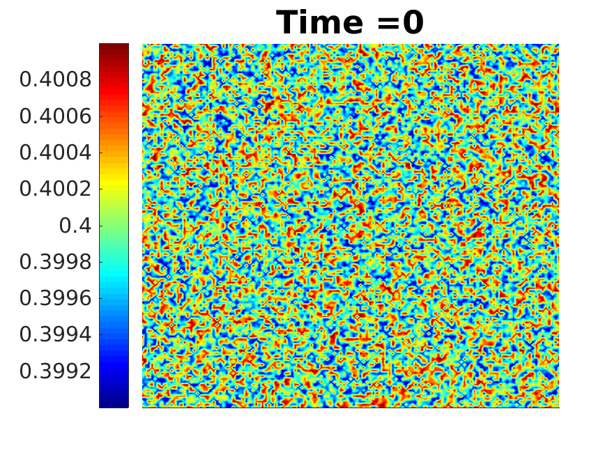
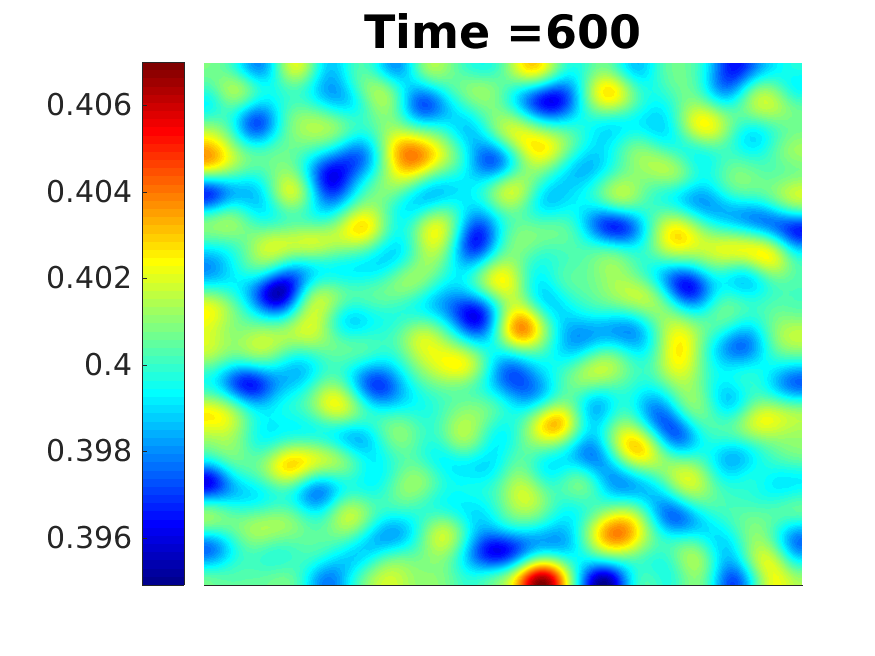
Refer to caption
(a)
Refer to caption
(b)
Refer to caption
(c)
Refer to caption
(d)
Refer to caption
(e)
Refer to caption
(f)
Figure 1: Experiment 1: Spinodal decomposition, time evolution of the volume fraction ϕ\phi.
Refer to caption
(a)
Refer to caption
(b)
Refer to caption
(c)
Refer to caption
(d)
Figure 2: Experiment 1: Spinodal decomposition, time evolution of the velocity norm |𝐮|2|\mathbf{u}|_{2}.
Refer to caption
(a)
Refer to caption
(b)
Refer to caption
(c)
Refer to caption
(d)
Refer to caption
(e)
Refer to caption
(f)
Refer to caption
(g)
Refer to caption
(h)
Refer to caption
(i)
Refer to caption
(j)
Refer to caption
(k)
Refer to caption
(l)
Figure 3: Experiment 1: Spinodal decomposition, time evolution of the bulk stress qq (top), pressure pp (middle) and chemical potential μ\mu (bottom).
Refer to caption
(a)
Refer to caption
(b)
Refer to caption
(c)
Refer to caption
(d)
Refer to caption
(e)
Refer to caption
(f)
Figure 4: Experiment 1: Time evolution of the total energy Et​o​tE_{tot} and the corresponding energy components Ek​i​n=12​∫|u|2,E_{kin}=\frac{1}{2}\int\left|u\right|^{2}, Ee​l=14​∫tr​(𝐂)2−2​tr​(log⁡(𝐂))E_{el}=\frac{1}{4}\int\mathrm{tr}(\mathbf{C})^{2}-2\mathrm{tr}(\log(\mathbf{C})), Eb​u​l​k=12​∫|q|2E_{bulk}=\frac{1}{2}\int\left|q\right|^{2}, Em​i​x=∫c02​|∇ϕ|2+F⁡(ϕ)E_{mix}=\int\frac{c_{0}}{2}\left|\nabla\phi\right|^{2}~+~F(\phi). The last picture demonstrates that the numerical scheme preserves mass 1|Ω|​∫ϕ\frac{1}{\left|\Omega\right|}\int\phi up to small error 1|Ω|​∫(ϕ⁡(x,0)−ϕ⁡(x,t))​𝑑x\frac{1}{\left|\Omega\right|}\int\left(\phi(x,0)-\phi(x,t)\right)\,\mathrm{d}x of the order 10−910^{-9}.

Experiment 2: The next simulation differs only in the potential and the initial condition for the conformation tensor. More precisely, we have now used the Flory-Huggins potential with np=ns=1​ and ​χ=28/11n_{p}=n_{s}=1\text{ and }\chi=28/11 and 𝐂0=𝐈\mathbf{C}_{0}=\mathbf{I}. We observe similar phase evolution as in Experiment 1 but on a different timescale. We can notice that simulations with the Flory Huggins potential are roughly twice faster than with the Ginzburg-Landau potential.
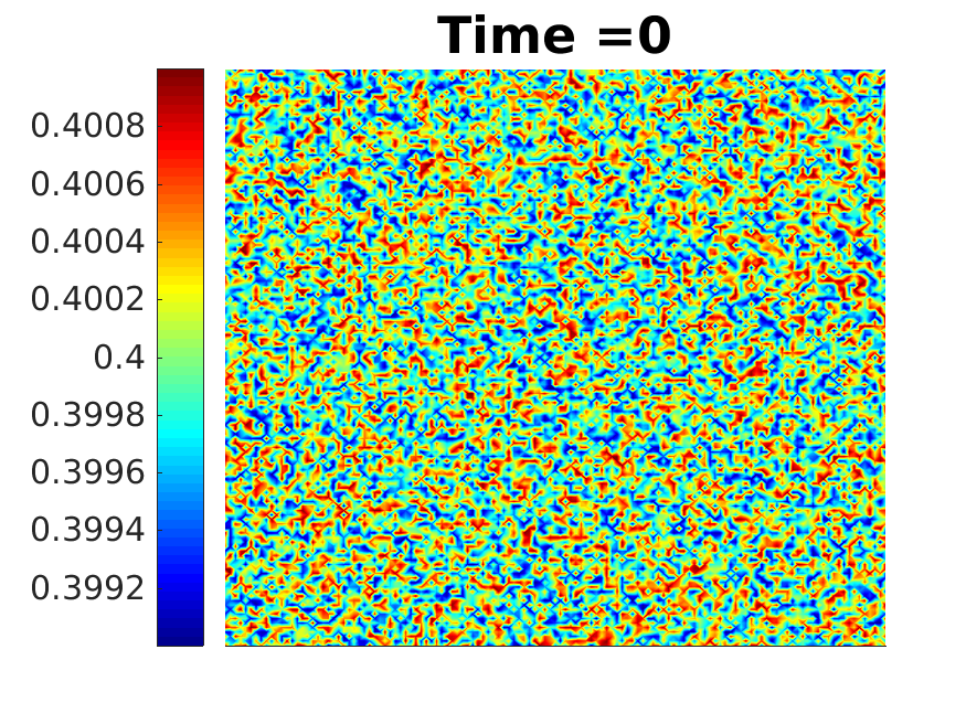
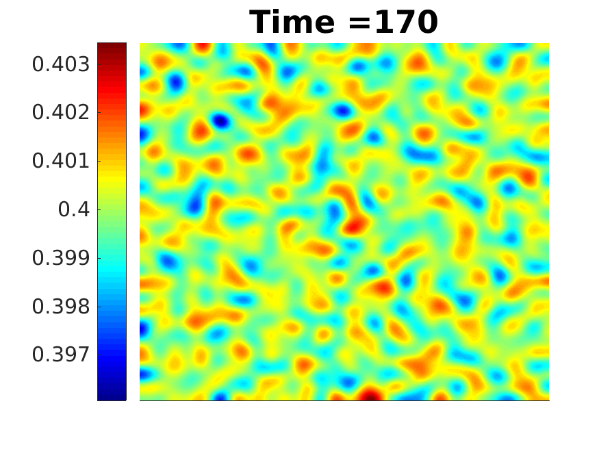
Refer to caption
(a)
Refer to caption
(b)
Refer to caption
(c)
Refer to caption
(d)
Refer to caption
(e)
Refer to caption
(f)
Figure 5: Experiment 2: Spinodal decomposition, time evolution of the volume fraction ϕ\phi.
Refer to caption
(a)
Refer to caption
(b)
Refer to caption
(c)
Refer to caption
(d)
Figure 6: Experiment 2: Spinodal decomposition, time evolution of the velocity norm |𝐮|2|\mathbf{u}|_{2}.
Refer to caption
(a)
Refer to caption
(b)
Refer to caption
(c)
Refer to caption
(d)
Refer to caption
(e)
Refer to caption
(f)
Refer to caption
(g)
Refer to caption
(h)
Refer to caption
(i)
Refer to caption
(j)
Refer to caption
(k)
Refer to caption
(l)
Figure 7: Experiment 2: Spinodal decomposition, time evolution of the bulk stress qq (top), pressure pp (middle) and chemical potential μ\mu (bottom).
Refer to caption
(a)
Refer to caption
(b)
Refer to caption
(c)
Refer to caption
(d)
Refer to caption
(e)
Refer to caption
(f)
Figure 8: Experiment 2: Time evolution of the total energy Et​o​tE_{tot} and the corresponding energy components. The last picture demonstrates that the numerical scheme preserves mass 1|Ω|​∫ϕ\frac{1}{\left|\Omega\right|}\int\phi up to small error of the order 10−710^{-7}.

Experiment 3: In this test we want to study the influence of non-zero initial velocity on the dynamics of the system with the Ginzburg-Landau potential. We denote by 𝟙B\mathds{1}_{B} the characteristic function of a ball with the radius 5050 and midpoint (64,64)(64,64). The initial conditions are
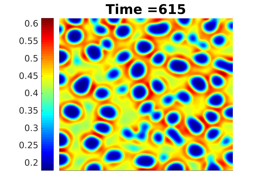
𝐮1=y−64128​𝟙B​(x,y),𝐮2=64−x128​𝟙B​(x,y),𝐂11=𝐂22=2,𝐂12=0.5.\displaystyle\mathbf{u}_{1}=\frac{y-64}{128}\mathds{1}_{B}(x,y),\qquad\mathbf{u}_{2}=\frac{64-x}{128}\mathds{1}_{B}(x,y),\qquad\mathbf{C}_{11}=\mathbf{C}_{22}=2,\mathbf{C}_{12}=0.5.

All other initial data are the same as in the previous experiments.
In Figure 9 we can recognize typical phase separation patterns as in the previous experiments. However, their evolution is much faster than in Experiment 1 which is due to the initial velocity field. In fact the phases occur now at similar times as in Experiment 2. This effect can be related to the so-called shear-induced phase separation. In Figure 10 we can observe the slow down of the vector field up to t≈750t\approx 750 and then the dispersion of the initial rotation. At this point the phase separation effects start to dominate the rotation and therefore we observe similar patterns as in Experiment 1 and 2.

Refer to caption
(a)
Refer to caption
(b)
Refer to caption
(c)
Refer to caption
(d)
Refer to caption
(e)
Refer to caption
(f)
Figure 9: Experiment 3: Spinodal decomposition, time evolution of the volume fraction ϕ\phi.
Refer to caption
(a)
Refer to caption
(b)
Refer to caption
(c)
Refer to caption
(d)
Refer to caption
(e)
Refer to caption
(f)
Refer to caption
(g)
Refer to caption
(h)
Figure 10: Experiment 3: Spinodal decomposition, time evolution of the velocity norm |𝐮|2|\mathbf{u}|_{2}.
Refer to caption
(a)
Refer to caption
(b)
Refer to caption
(c)
Refer to caption
(d)
Refer to caption
(e)
Refer to caption
(f)
Figure 11: Experiment 3: Time evolution of the total energy Et​o​tE_{tot} and the corresponding energy components. The last picture demonstrates that the numerical scheme preserves mass 1|Ω|​∫ϕ\frac{1}{\left|\Omega\right|}\int\phi up to small error 1|Ω|​∫(ϕ⁡(x,0)−ϕ⁡(x,t))​𝑑x\frac{1}{\left|\Omega\right|}\int\left(\phi(x,0)-\phi(x,t)\right)\,\mathrm{d}x of the order 10−910^{-9}.

10 Conclusion and Outlook

In this paper we have analyzed mathematical properties of the viscoelastic phase separation model (2.6) that has been proposed in [55]. Instead of the Oldroyd-B equations for the time evolution of viscoelastic stress tensor we have used a more general Peterlin model as proposed in [39].
A regular potential for the phase separation, i.e. the Ginzburg-Landau potential, allowed us to prove the existence of global weak solutions to (2.6). To this end we had to modify slightly the original model of [55] by introducing a parameter κ∈[0,1)\kappa\in[0,1) in front of the viscous coupling terms in the equations for volume fraction ϕ\phi and bulk stress qq, see (2.6)1,(2.6)2(\ref{eq:full_model})_{1},(\ref{eq:full_model})_{2}, respectively. We have derived the necessary a priori estimates and passed to the limit in the Galerkin approximations. Applicability of the model (2.6) to describe complex dynamics of spinodal decomposition has been documented by numerical experiments presented in Section 9, see, also [50]. Our numerical experiments demonstrate that the choice κ=1\kappa=1 makes no problem for the existence of a weak solution in practice. Therefore, it will be interesting to investigate in the future whether analogous existence results hold also for κ→1\kappa\rightarrow 1.
Building on the present study our next goal is to investigate a degenerate model with the Flory-Huggins potential and degenerate mobilities, see [12].

Acknowledgement

This research was supported by the German Science Foundation (DFG) under the Collaborative Research Center TRR 146 Multiscale Simulation Methods for Soft Matters (Project C3) and partially by the VEGA grant 1/0684/17 and the Mainz Institute of Multiscale Modeling (M3odel). We would like to thank B. Dünweg, D. Spiller and J. Kat’uchová for fruitful discussions on the topic.

11 Appendix

11.1 Model derivation

The aim of this section is to discuss a derivation of the viscoelastic phase separation model (2.6). Systematic model derivation and further discussions on various model variants can be found in our recent works [3, 11]. A complete rigorous derivation from a microscopic description is however not yet available in the literature.

To keep our paper self-consistent we present important steps of the model derivation. First, as it is standardly used, cf. [28, 29, 55], the derivation of a thermodynamically consistent model is divided into the description of reversible and irreversible dynamics. The reversible part can be obtained by the virtual work principle [20], while the irreversible part will be treated in a dissipative setting as in [30]. Our further discussion is structured in the following way.

  1. 1.

    Discussion on the free energy and introduction of a conservative model.

  2. 2.

    Consideration of non-equilibrium dynamics using the relative velocity 𝐰\mathbf{w}.

  3. 3.

    Consideration of dissipative effects.

11.2 Free energy and a conservative model

First, we review the energy of the original viscoelastic phase separation model from [55] rewritten using the conformation tensor 𝐂.\mathbf{C}. The total energy reads

E\displaystyle E =∫F⁡(ϕ)+c02​|∇ϕ|2+∫12​|𝐮|2+∫12​q2+12​∫tr⁡(𝐂),\displaystyle=\int F(\phi)+\frac{c_{0}}{2}|\nabla\phi|^{2}+\int\frac{1}{2}|\mathbf{u}|^{2}+\int\frac{1}{2}q^{2}+\frac{1}{2}\int\mathrm{tr}({\mathbf{C}}),

where F⁡(ϕ)F(\phi) denotes an appropriate mixing potential such as (2.2) or (2.3). The first integral represents the mixing energy, while the second stands for the total kinetic energy. We note that the last integral represents the free energy modeled by the viscoelastic conformation tensor. Following [51] the second last term models the energy contribution due to the bulk stress q​𝐈.q\mathbf{I}. The latter originates from (microscopic) intermolecular attractive interactions and can be seen as additional viscoelastic pressure. We refer a reader to our recent work [11] for a more detailed and physically motivated discussion on the connection between the conformation stress tensor 𝐂\mathbf{C} and q​𝐈q\mathbf{I}. Indeed, the conformation tensor 𝐂\mathbf{C} is connected to the viscoelastic effects of the volume-averaged velocity 𝐮\mathbf{u} and q​𝐈q\mathbf{I} is connected to the relative velocity 𝐰=𝐮p−𝐮s.\mathbf{w}=\mathbf{u}_{p}-\mathbf{u}_{s}. Here 𝐮p,𝐮s\mathbf{u}_{p},\mathbf{u}_{s} are the velocities of polymer and solvent phases, respectively.

We proceed with formulating the total energy of our desired model by

E\displaystyle E =∫F⁡(ϕ)+c02​|∇ϕ|2+∫12​|𝐮|2+∫12​q2+∫14​tr​(𝐂)2−12​tr​(ln⁡(𝐂)).\displaystyle=\int F(\phi)+\frac{c_{0}}{2}|\nabla\phi|^{2}+\int\frac{1}{2}|\mathbf{u}|^{2}+\int\frac{1}{2}q^{2}+\int\frac{1}{4}\mathrm{tr}({\mathbf{C}})^{2}-\frac{1}{2}\mathrm{tr}({\ln(\mathbf{C})}). (11.1)

We note that the quadratic term in the last integral results from a nonlinear dependence of the viscoelastic stress tensor on the conformation tensor and the term −tr⁡(ln⁡(𝐂))-\mathrm{tr}({\ln(\mathbf{C})}) represents the free energy of non-interacting macro-molecules, see [54] and [2]. This choice of the elastic energy yields a phase separation model, where viscoelastic effects are described by the Peterlin model. The latter was extensively studied in our recent works [38, 39, 44] both from the analytical and numerical point of view. We note that this viscoelastic model has been also derived as a rigorous closure of a kinetic model in [32]. The derivation of a full viscoelastic phase separation model presented below is general and applicable also to other choices of the elastic energy, see, e.g., [41] for the FENE-P model or [40] for a generalized Peterlin model. Using such generalizations within a full phase separation model is an interesting topic for future research.

The conservative dynamics of viscoelastic phase separation can be derived applying the Poisson bracket formalism, as presented in [3]. In general, one should derive a compressible model via the standard Poisson brackets and afterwards apply a reduction to an incompressible model, similar to a derivation presented in [3]. Such an approach yields the following basic equations, see [11],

∂∂t​ϕ\displaystyle\frac{\partial}{\partial t}\phi +𝐮⋅∇ϕ=0,\displaystyle+\mathbf{u}\cdot\nabla\phi=0,
∂∂t​𝐮\displaystyle\frac{\partial}{\partial t}\mathbf{u} +(𝐮⋅∇𝐮)−∇p=−c0​div​(∇ϕ⊗∇ϕ)−div⁡(2​𝐂​δ​Eδ​𝐂),div⁡(𝐮)=0,\displaystyle+(\mathbf{u}\cdot\nabla\mathbf{u})-\nabla p=-c_{0}\mathrm{div}\left({\nabla\phi\otimes\nabla\phi}\right)-\mathrm{div}\left({2\mathbf{C}\frac{\delta E}{\delta\mathbf{C}}}\right),\quad\mathrm{div}\left({\mathbf{u}}\right)=0,
∂∂t​q\displaystyle\frac{\partial}{\partial t}q +𝐮⋅∇q=0,\displaystyle+\mathbf{u}\cdot\nabla q=0,
D▽​𝐂Dt≡∂∂t​𝐂\displaystyle\frac{\mathrm{\overset{\triangledown}{D}}\mathbf{C}}{\mathrm{Dt}}\equiv\frac{\partial}{\partial t}\mathbf{C} +(𝐮⋅∇)𝐂−∇𝐮𝐂−𝐂∇𝐮⊤=0.\displaystyle+(\mathbf{u}\cdot\nabla)\mathbf{C}-\nabla\mathbf{u}\mathbf{C}-\mathbf{C}\nabla\mathbf{u}^{\top}=0. (11.2)

It can be shown that formally the model conserves the free energy given by (11.1). Clearly, model (11.2) only describes the reversible part of the dynamics.

11.3 Closure relation for the relative velocity

In what follows we introduce the relative velocity 𝐰\mathbf{w}. The conservative model (11.2) can be understand as a reduced model with 𝐰=0\mathbf{w}=0. Following our derivation in [11] q​𝐈q\mathbf{I} is associated with the divergence of 𝐰\mathbf{w}, while the viscoelastic stress tensor 𝐓\mathbf{T} arising from 𝐂\mathbf{C}, i.e. 𝐓=tr⁡(𝐂)​𝐂−𝐈\mathbf{T}=\mathrm{tr}(\mathbf{C})\mathbf{C}-\mathbf{I}, is associated to the deformation gradient of the velocity 𝐮\mathbf{u}. Finally, due to the divergence-freedom of the velocity 𝐮\mathbf{u} there is no relevant stress associated with div⁡(𝐮)\mathrm{div}\left({\mathbf{u}}\right). This will be include via the linear term A1​(ϕ)​div​(𝐰)A_{1}(\phi)\mathrm{div}\left({\mathbf{w}}\right) into qq. A short calculation shows that for the upper convected derivative D▽​𝐈Dt=2​D​𝐮\frac{\mathrm{\overset{\triangledown}{D}}\mathbf{I}}{\mathrm{Dt}}=2\mathrm{D}\mathbf{u}, hence an evolution equation for the viscoelastic stress tensor 𝐓\mathbf{T} already includes a dependence on the deformation gradient.

Using the relative velocity we obtain the following equations from (11.2)

∂∂t​ϕ\displaystyle\frac{\partial}{\partial t}\phi +𝐮⋅∇ϕ=−div(ϕ(1−ϕ)𝐰),\displaystyle+\mathbf{u}\cdot\nabla\phi=-\textrm{div}\big(\phi(1-\phi)\mathbf{w}\big),
∂∂t​𝐮\displaystyle\frac{\partial}{\partial t}\mathbf{u} +(𝐮⋅∇𝐮)−∇p=−c0​div​(∇ϕ⊗∇ϕ)−div⁡(tr⁡(𝐂)​𝐂),div⁡(𝐮)=0,\displaystyle+(\mathbf{u}\cdot\nabla\mathbf{u})-\nabla p=-c_{0}\mathrm{div}\left({\nabla\phi\otimes\nabla\phi}\right)-\mathrm{div}\left({\mathrm{tr}(\mathbf{C})\mathbf{C}}\right),\quad\mathrm{div}\left({\mathbf{u}}\right)=0,
∂∂t​q\displaystyle\frac{\partial}{\partial t}q +𝐮⋅∇q=A1(ϕ)div(𝐰),\displaystyle+\mathbf{u}\cdot\nabla q=A_{1}(\phi)\mathrm{div}\left({\mathbf{w}}\right),
∂∂t​𝐂\displaystyle\frac{\partial}{\partial t}\mathbf{C} +(𝐮⋅∇)𝐂−∇𝐮𝐂−𝐂∇𝐮⊤=0.\displaystyle+(\mathbf{u}\cdot\nabla)\mathbf{C}-\nabla\mathbf{u}\mathbf{C}-\mathbf{C}\nabla\mathbf{u}^{\top}=0. (11.3)

We already know that the model is conservative for 𝐰=0\mathbf{w}=0. In order to close the system we will choose a suitable closure relation for 𝐰\mathbf{w}, which is based on the second law of thermodynamics. Computing the change of the free energy (11.1) yields

ddt​E​(ϕ,q,𝐮,𝐂)\displaystyle\frac{\mathrm{d}}{\mathrm{dt}}E(\phi,q,\mathbf{u},\mathbf{C}) =∫Ωϕ(1−ϕ)𝐰∇δ​Eδ​ϕ−𝐰⋅∇(A(ϕ)q)\displaystyle=\int_{\Omega}\phi(1-\phi)\mathbf{w}\nabla\frac{\delta E}{\delta\phi}-\mathbf{w}\cdot\nabla(A(\phi)q)
=∫Ω𝐰⋅[ϕ(1−ϕ)∇δ​Eδ​ϕ−∇(A(ϕ)q)].\displaystyle=\int_{\Omega}\mathbf{w}\cdot\Big[\phi(1-\phi)\nabla\frac{\delta E}{\delta\phi}-\nabla(A(\phi)q)\Big]. (11.4)

Hence, the above expression is non-negative for 𝐰=−[ϕ(1−ϕ)∇δ​Eδ​ϕ−∇(A(ϕ)q)]\mathbf{w}=-[\phi(1-\phi)\nabla\frac{\delta E}{\delta\phi}-\nabla(A(\phi)q)]. We again refer to [11] where we have showed that such a term arises even in more general processes based on the relative velocity 𝐰\mathbf{w}. Note that the model reduction by choosing a closure relation for 𝐰\mathbf{w} introduces dissipation into the system.

11.4 Dissipative part

In this part, we will introduce additional physically motivated dissipation terms. First, we add a diffusive term to the equations of the conformation tensor 𝐂\mathbf{C}. As mentioned in the introduction the existence of such a diffusive term in thermodynamically consistent viscoelastic models has been investigated and verified in [1, 45]. Furthermore, we add Navier-Stokes-type viscosity terms to the momentum equations.

Since both q​𝐈,𝐂q\mathbf{I},\mathbf{C} are modeling the viscoelastic effects, we expect them to decay to an equilibrium in the absence of all forces, which will be modeled by the relaxation terms. The generic form for such a relaxation is given by

−1τs​(ϕ)​g​(𝐂)​δ​Eδ​𝐂, or −1τb​(ϕ)​g​(q)​q.-\frac{1}{\tau_{s}(\phi)}g(\mathbf{C})\frac{\delta E}{\delta\mathbf{C}},\text{ or }-\frac{1}{\tau_{b}(\phi)}g(q)q.

We note in passing that in order to preserve frame invariant structure, the choice of g⁡(𝐂)g(\mathbf{C}) is restricted. In our work we have opted for the Peterlin model, i.e. we choose g⁡(𝐂)=tr⁡(𝐂)​𝐂g(\mathbf{C})=\mathrm{tr}(\mathbf{C})\mathbf{C}. For the bulk stress we choose the simplest available mechanism, i.e. g⁡(q)=1g(q)=1. Altogether we obtain the following resulting system

D​ϕDt\displaystyle\frac{\mathrm{D}\phi}{\mathrm{Dt}} =div(ϕ2(1−ϕ)2∇δ​Eδ​ϕ−ϕ(1−ϕ)∇(A(ϕ)q)),\displaystyle=\mathrm{div}\left({\phi^{2}(1-\phi)^{2}\nabla\frac{\delta E}{\delta\phi}-\phi(1-\phi)\nabla(A(\phi)q)}\right),
D​qDt\displaystyle\frac{\mathrm{D}q}{\mathrm{Dt}} =−1τb​(ϕ)q+A1(ϕ)div(∇(A(ϕ)q)−ϕ(1−ϕ)∇δ​Eδ​ϕ),\displaystyle=-\frac{1}{\tau_{b}(\phi)}q+A_{1}(\phi)\mathrm{div}\left({\nabla(A(\phi)q)-\phi(1-\phi)\nabla\frac{\delta E}{\delta\phi}}\right), (11.5)
D​𝐮Dt\displaystyle\frac{\mathrm{D}\mathbf{u}}{\mathrm{Dt}} =div⁡(η⁡(ϕ)​D​𝐮)−∇p−c0​div​(∇ϕ⊗∇ϕ)−div⁡(tr⁡(𝐂)​𝐂),div⁡(𝐮)=0,\displaystyle=\mathrm{div}\left({\eta(\phi)\mathrm{D}\mathbf{u}}\right)-\nabla p-c_{0}\mathrm{div}\left({\nabla\phi\otimes\nabla\phi}\right)-\mathrm{div}\left({\mathrm{tr}(\mathbf{C})\mathbf{C}}\right),\hskip 14.22636pt\mathrm{div}\,{(}\mathbf{u})=0,
D▽​𝐂Dt\displaystyle\frac{\mathrm{\overset{\triangledown}{D}}\mathbf{C}}{\mathrm{Dt}} =−1τs​(ϕ)​tr​(𝐂)​(tr⁡(𝐂)​𝐂−𝐈)+ε​Δ​𝐂.\displaystyle=-\frac{1}{\tau_{s}(\phi)}\mathrm{tr}(\mathbf{C})(\mathrm{tr}(\mathbf{C})\mathbf{C}-\mathbf{I})+\varepsilon\Delta\mathbf{C}.

11.5 Reformulation and remarks

In this subsection, we will suitably reformulate (11.5) to obtain our model (2.6).

First, the Leslie-Erickson stress tensor −c0​div​(∇ϕ⊗∇ϕ)-c_{0}\mathrm{div}\left({\nabla\phi\otimes\nabla\phi}\right) can be rewritten according to [50]

−c0div(∇ϕ⊗∇ϕ)=μ∇ϕ−∇(c02|∇ϕ|2+F(ϕ)),-c_{0}\mathrm{div}\left({\nabla\phi\otimes\nabla\phi}\right)=\mu\nabla\phi-\nabla\bigg(\frac{c_{0}}{2}|\nabla\phi|^{2}+F(\phi)\bigg),

where the second term can be absorbed into the pressure pp. Reordering and expanding terms with the choices

m⁡(ϕ)=ϕ2​(1−ϕ)2,n⁡(ϕ)=ϕ⁡(1−ϕ),τs​(ϕ)−1=h⁡(ϕ),f⁡(ϕ)=∂ℱ∂ϕ,𝐓=tr⁡(𝐂)​𝐂,m(\phi)=\phi^{2}(1-\phi)^{2},\;\;n(\phi)=\phi(1-\phi),\;\;\tau_{s}(\phi)^{-1}=h(\phi),\;\;f(\phi)=\frac{\partial\mathcal{F}}{\partial\phi},\;\;\mathbf{T}=\mathrm{tr}(\mathbf{C})\mathbf{C},

yields the desired system governing viscoelastic phase separation.

∂ϕ∂t+𝐮⋅∇ϕ=div(m(ϕ)∇μ)−div(n(ϕ)∇(A(ϕ)q))∂q∂t+𝐮⋅∇q=−1τb​(ϕ)q+A(ϕ)div(∇(A(ϕ)q))−A(ϕ)div(n(ϕ)∇μ)∂𝐮∂t+(𝐮⋅∇)𝐮=div(η(ϕ)(∇𝐮+(∇𝐮)T))−∇p+div(𝐓)+μ∇ϕ∂𝐂∂t+(𝐮⋅∇)𝐂=(∇𝐮)​𝐂+𝐂​(∇𝐮)T+h⁡(ϕ)​tr​(𝐂)​𝐈−h⁡(ϕ)​tr​(𝐂)2​𝐂+ε​Δ​𝐂div⁡(𝐮)=0𝐓=tr⁡(𝐂)​𝐂μ=−c0​Δ​ϕ+f⁡(ϕ)\displaystyle\begin{split}\frac{\partial\phi}{\partial t}+\mathbf{u}\cdot\nabla\phi&=\mathrm{div}\left({m(\phi)\nabla\mu}\right)-\mathrm{div}\left({n(\phi)\nabla\big(A(\phi)q\big)}\right)\\ \frac{\partial q}{\partial t}+\mathbf{u}\cdot\nabla q&=-\frac{1}{\tau_{b}(\phi)}q+A(\phi)\mathrm{div}\left({\nabla\big(A(\phi)q\big)}\right)-A(\phi)\mathrm{div}\left({n(\phi)\nabla\mu}\right)\\ \frac{\partial\mathbf{u}}{\partial t}+(\mathbf{u}\cdot\nabla)\mathbf{u}&=\mathrm{div}\left({\eta(\phi)\Big(\nabla\mathbf{u}+(\nabla\mathbf{u})^{T}\Big)}\right)-\nabla p+\mathrm{div}\,{(}\mathbf{T})+\mu\nabla\phi\\ \frac{\partial\mathbf{C}}{\partial t}+(\mathbf{u}\cdot\nabla)\mathbf{C}&=(\nabla\mathbf{u})\mathbf{C}+\mathbf{C}(\nabla\mathbf{u})^{T}+h(\phi)\mathrm{tr}(\mathbf{C})\mathbf{I}-h(\phi)\mathrm{tr}(\mathbf{C})^{2}\mathbf{C}+\varepsilon\Delta\mathbf{C}\\ \mathrm{div}\,{(}\mathbf{u})&=0\hskip 28.45274pt\mathbf{T}=\mathrm{tr}\left({\mathbf{C}}\right)\mathbf{C}\hskip 28.45274pt\mu=-c_{0}\Delta\phi+f(\phi)\end{split} (11.6)

A formal proof of thermodynamic consistency of (11.6) is given in Theorem 3.2 with κ=1\kappa=1.

Remark 11.1.

We note that the above derivation of model (11.6) is consistent with the GENERIC formalism [29, 28, 11, 3]. GENERIC (general equation for the non-equilibrium reversible–irreversible coupling) is a well-accepted framework for the derivation of thermodynamically admissible evolution equations for non-equilibrium systems. Analogously, one can consider the approach proposed recently by Málek et al. [45, 46] and derive a thermodynamically consistent model by prescribing the state variables, here (ϕ,q,𝐮,𝐂)(\phi,q,\mathbf{u},\mathbf{C}), a free energy and a dissipation process modeling the energy dissipation. The free energy is given by

E\displaystyle E =∫F⁡(ϕ)+c02​|∇ϕ|2+∫12​|𝐮|2+∫12​q2+∫14​tr​(𝐂)2−12​tr​(ln⁡(𝐂))\displaystyle=\int F(\phi)+\frac{c_{0}}{2}|\nabla\phi|^{2}+\int\frac{1}{2}|\mathbf{u}|^{2}+\int\frac{1}{2}q^{2}+\int\frac{1}{4}\mathrm{tr}({\mathbf{C}})^{2}-\frac{1}{2}\mathrm{tr}({\ln(\mathbf{C})})

and dissipation process by

∫ζ\displaystyle\int\zeta =∫|n(ϕ)∇δ​Eδ​ϕ−∇(A(ϕ)q)|2+η⁡(ϕ)2|∇𝐮+(∇𝐮)T|2+1τb​(ϕ)q2\displaystyle=\int\left|n(\phi)\nabla\frac{\delta E}{\delta\phi}-\nabla(A(\phi)q)\right|^{2}+\frac{\eta(\phi)}{2}\left|\nabla\mathbf{u}+(\nabla\mathbf{u})^{T}\right|^{2}+\frac{1}{\tau_{b}(\phi)}q^{2}
+h⁡(ϕ)2tr(𝐓)tr(𝐓+𝐓−1−2𝐈)+ε2|∇tr(𝐂)|2−ε2∇𝐂:∇𝐂−1.\displaystyle\hskip 28.45274pt+\frac{h(\phi)}{2}\mathrm{tr}({\mathbf{T}})\mathrm{tr}({\mathbf{T}+\mathbf{T}^{-1}-2\mathbf{I}})+\frac{\varepsilon}{2}|\nabla\mathrm{tr}(\mathbf{C})|^{2}-\frac{\varepsilon}{2}\nabla\mathbf{C}:\nabla\mathbf{C}^{-1}.

As pointed out above the conservative part of the model, i.e. (11.2), can be derived by means of the Poisson bracket formalism using only the state variables and the free energy, i.e. the dissipation process is zero. In the second step, the dissipative contributions are incorporated using a non-zero dissipation process.

As one can quickly recognize (11.6) differs only slightly from the studied model (2.6). The energy dissipation (11.4) yields the estimate

ϕ(1−ϕ)∇μ−∇(A(ϕ)q)∈L2(0,T;L2(Ω)).\phi(1-\phi)\nabla\mu-\nabla\big(A(\phi)q\big)\in L^{2}(0,T;L^{2}(\Omega)).

However, we do not have independent a priori estimates for ∇μ\nabla\mu and ∇(A⁡(ϕ)​q)\nabla(A(\phi)q). This is due to the cross-diffusion structure in the (ϕ,q)(\phi,q) subsystem. A typical technique to deal with such problems is to dominate the cross-diffusion by a diagonal diffusion. To cure this problem we have introduced in (11.6) a parameter κ∈[0,1)\kappa\in[0,1), i.e. n⁡(ϕ):=κ​n​(ϕ)n(\phi):=\kappa n(\phi) which leads to our final viscoelastic phase separation model (2.6).

References

  • [1] W. J. Barrett and E. Süli. Existence and equilibration of global weak solutions to kinetic models for dilute polymers I: Finitely extensible nonlinear bead-spring chains. Math. Models Methods Appl. Sci., 21(6):1211-1289, 2011.
  • [2] D. Hu and T. Lelièvre. New entropy estimates for the Oldroyd-B model and related models. Commun. Math. Sci., 5(4):909-916, 2007.
  • [3] D. Spiller and A. Brunk and O. Habrich and H. Egger and M. Lukáčová-Medvid’ová and Burkhard Dünweg. Systematic derivation of hydrodynamic equations for viscoelastic phase separation. J. Phys.: Condens. Matter., 33 364001, 2021.
  • [4] H. Abels. On a diffuse interface model for two-phase flows of viscous, incompressible fluids with matched densities. Arch. Ration. Mech. An., 194(2):463–506, 2009.
  • [5] H. Abels, D. Depner, and H. Garcke. On an incompressible Navier–Stokes/Cahn–Hilliard system with degenerate mobility. Ann. I H Poincare-An., 30(6):1175–1190, 2013.
  • [6] H. Abels and E. Feireisl. On a diffuse interface model for a two-phase flow of compressible viscous fluids. Indiana U. Math. J., (57):659–698, 2008.
  • [7] S. Agmon. Lectures on Elliptic Boundary Value Problems. AMS Chelsea Publishing. AMS, Providence, 2010.
  • [8] J. W. Barrett and E. Süli. Existence of large-data global-in-time finite-energy weak solutions to a compressible FENE-P model. Math. Mod. Meth. Appl. S, 28(10):1929–2000, 2018.
  • [9] F. Boyer. Mathematical study of multiphase flow under shear through order parameter formulation. Asymptotic Anal., (20):175–212, 1999.
  • [10] F. Brezzi and J. Pitkäranta. On the stabilization of finite element approximations of the Stokes equations. In Hackbusch - Efficient Solutions of Elliptic Systems, pages 11–19. 1984.
  • [11] A. Brunk, B. Dünweg, H. Egger, O. Habrich, M. Lukáčová-Medvid’ová, and D. Spiller. Analysis of a viscoelastic phase separation model. J. Phys.: Condens. Matter, 33 234002, 2021.
  • [12] A. Brunk and M. Lukáčová-Medvid’ová. Global existence of weak solutions to viscoelastic phase separation: Part II Degenerate Case, preprint. 2019.
  • [13] L. Cherfils, A. Miranville, and S. Zelik. The Cahn-Hilliard equation with logarithmic potentials. Milan J. Math., 79(2):561–596, 2011.
  • [14] L. Chupin. Existence result for a mixture of non Newtonian flows with stress diffusion using the Cahn-Hilliard formulation. DCDS-B, 3(1):45–68, 2003.
  • [15] P. G. Ciarlet. The Finite Element Method for Elliptic Problems, volume 40 of Classics in Applied Mathematics. SIAM, Philadelphia, 2002.
  • [16] P. Colli, S. Frigeri, and M. Grasselli. Global existence of weak solutions to a nonlocal Cahn–Hilliard–Navier–Stokes system. J. Math. Anal. Appl., 386(1):428–444, 2012.
  • [17] S. Dai and Q. Du. Weak solutions for the Cahn–Hilliard equation with degenerate mobility. Arch. Ration. Mech. An., 219(3):1161–1184, 2016.
  • [18] P. Degond, H. Liu. Kinetic models for polymers with inertial effects. Netw. Heterog. Media 4:625–-647, 2009.
  • [19] A. E. Diegel, C. Wang, and S. M. Wise. Stability and convergence of a second-order mixed finite element method for the Cahn–Hilliard equation. IMA J. Numer. Anal., 36(4):1867–1897, 2016.
  • [20] M. Doi and S. F. Edwards. The Theory of Polymer Dynamics, volume 73 of International Series of Monographs on Physics. Oxford, 2007.
  • [21] C. M. Elliott. The Cahn-Hilliard model for the kinetics of phase separation. In J.-F. Rodrigues, editor, Mathematical Models for Phase Change Problems, Int. S. Num. M., pages 35–73. Birkhäuser, 1989.
  • [22] C. M. Elliott and H. Garcke. On the Cahn–Hilliard equation with degenerate mobility. SIAM J. Math. Anal., 27(2):404–423, 1996.
  • [23] E. Feireisl. On weak solutions to a diffuse interface model of a binary mixture of compressible fluids. DCDS-S, 9(1):173–183, 2016.
  • [24] G. B. Folland. Real analysis: Modern Techniques and their Applications. Pure A Math. John Wiley & Sons, New York, 2011.
  • [25] S. Frigeri, M. Grasselli, and E. Rocca. A diffuse interface model for two-phase incompressible flows with non-local interactions and non-constant mobility. Nonlinearity, 28(5):1257, 2015.
  • [26] G. Giacomin and J. L. Lebowitz. Phase segregation dynamics in particle systems with long range interactions. I. Macroscopic limits. J. Stat. Phys., 87(1-2):37–61, 1997.
  • [27] G. Giacomin and J. L. Lebowitz. Phase segregation dynamics in particle systems with long range interactions II: Interface motion. SIAM J. Appl. Math., 58(6):1707–1729, 1998.
  • [28] M. Grmela and H. C. Öttinger. Dynamics and thermodynamics of complex fluids. I. Development of a general formalism. Phys. Rev. E, 56(6):6620–6632, 1997.
  • [29] M. Grmela and H. C. Öttinger. Dynamics and thermodynamics of complex fluids. II. Illustrations of a general formalism. Phys. Rev. E, 56(6):6633–6655, 1997.
  • [30] S. R. d. Groot and P. Mazur. Non-equilibrium thermodynamics. Dover Books on Physics. Dover Publications, 2016.
  • [31] G. Grün. Degenerate parabolic differential equations of fourth order and a plasticity model with non-local hardening. Z. Anal. Anwend., 14(3):541–574, 1995.
  • [32] P. Gwiazda, M. Lukáčová-Medvid’ová, H. Mizerov á, A. S̀zwierczewska-Gwiazda. Existence of global weak solutions to the kinetic Peterlin model. Nonlinear Analysis: Real World App. 44:465–478, 2018.
  • [33] C. O. Horgan. Korn’s inequalities and their applications in continuum mechanics. SIAM Rev., 37(4):491–511, 1995.
  • [34] O. A. Ladyženskaja, V. A. Solonnikov, and N. N. Ural’ceva. Linear and Quasi-linear Equations of Parabolic Type, volume 23 of Translations of Mathematical Monographs. AMS, Providence, 1968.
  • [35] S.-O. Londen and H. Petzeltová. Regularity and separation from potential barriers for a non-local phase-field system. J. Math. Anal. App., 379(2):724–735, 2011.
  • [36] J. Lowengrub and L. Truskinovsky. Quasi–incompressible Cahn–Hilliard fluids and topological transitions. P. Roy. Soc. A-Math. Phy., 454(1978):2617–2654, 1998.
  • [37] M. Lukáčová-Medvid’ová, B. Dünweg, P. Strasser, and N. Tretyakov. Energy-stable numerical schemes for multiscale simulations of polymer–solvent mixtures. In P. van Meurs, M. Kimura, and H. Notsu, editors, Mathematical Analysis of Continuum Mechanics and Industrial Applications II, volume 30 of Math Ind, pages 153–165. Springer, 2017.
  • [38] M. Lukáčová-Medvid’ová, H. Mizerová, and Š. Nečasová. Global existence and uniqueness result for the diffusive Peterlin viscoelastic model. Nonlinear. Anal.-Theor., 120:154–170, 2015.
  • [39] M. Lukáčová-Medvid’ová, H. Mizerová, H. Notsu, and M. Tabata. Numerical analysis of the Oseen-type Peterlin viscoelastic model by the stabilized Lagrange–Galerkin method. Part II: A linear scheme. ESAIM: M2AN, 51(5):1663–1689, 2017.
  • [40] M. Lukáčová-Medvid’ová, H. Mizerová, Šárka Nečasová and Michael Renardy. Global existence result for the generalized Peterlin viscoelastic model. SIAM J. Math. Anal., 49(4), 2950–2964, 2017.
  • [41] N. Masmoudi. Global existence of weak solutions to macroscopic models of polymeric flows. J. Math. Pures Appl. 96:502–-520. 2011.
  • [42] S. Melchionna, H. Ranetbauer, and L. Trussardi. From nonlocal to local Cahn-Hilliard equation. http://arxiv.org.pdf/1803.09729v1.
  • [43] A. Miranville and S. Zelik. Robust exponential attractors for Cahn-Hilliard type equations with singular potentials. Math. Meth. Appl. Sci., 27(5):545–582, 2004.
  • [44] H. Mizerová. Analysis and numerical solution of the Peterlin viscoelastic model. Dissertation, Johannes Gutenberg-Universität, Mainz, 2015.
  • [45] J. Málek, V. Průša, T. Skřivan, and E. Süli. Thermodynamics of viscoelastic rate-type fluids with stress diffusion. Phys. Fluids, 30(2):023101, 2018.
  • [46] J. Málek, K. Rajagopal, and K. Tůma. On a variant of the Maxwell and Oldroyd-B models within the context of a thermodynamic basis. Int. J. Non. Linear Mech., 76:42 – 47, 2015.
  • [47] J. Nečas, J. Málek, M. Rokyta, and M. Růžička. Weak and Measure-Valued Solutions to Evolutionary PDEs, volume 13 of Appl. Math. Comput.. Chapman-Hall, 1996.
  • [48] H. Notsu and M. Tabata. Error estimates of a pressure-stabilized characteristics finite element scheme for the Oseen equations. J. Sci. Comput., 65(3):940–955, 2015.
  • [49] J. D. Shieber. Generalized Brownian configuration field for Fokker–Planck equations including center-of-mass diffusion. J. Non-Newton. Fluid Mech. 135:179–181, 2006.
  • [50] P. J. Strasser, G. Tierra, B. Dünweg, and M. Lukáčová-Medvid’ová. Energy-stable linear schemes for polymer–solvent phase field models. Comput. Math. Appl., 2018.
  • [51] H. Tanaka. Viscoelastic phase separation. J. Phys.: Condens. Matter, 12(15):R207.
  • [52] R. Temam. Navier-Stokes equations and nonlinear functional analysis, volume 41 of CBMS-NSF regional conference series in applied mathematics. SIAM, Philadelphia, 2 edition, 1983.
  • [53] R. Temam. Infinite-Dimensional Dynamical Systems in Mechanics and Physics, volume 68 of Applied Mathematical Sciences. Springer, 1997.
  • [54] P. Wapperom and M. A. Hulsen. Thermodynamics of viscoelastic fluids: The temperature equation. J. Rheol., 42(5):999–1019, 1998.
  • [55] D. Zhou, P. Zhang, and W. E. Modified models of polymer phase separation. Phys. Rev. E, 73(6):061801, 2006.