Graph Signal Processing – Part I: Graphs, Graph Spectra, and Spectral Clustering
Abstract
The area of Data Analytics on graphs promises a paradigm shift as we approach information processing of classes of data, which are typically acquired on irregular but structured domains (social networks, various ad-hoc sensor networks). Yet, despite its long history, current approaches mostly focus on the optimization of graphs themselves, rather than on directly inferring learning strategies, such as detection, estimation, statistical and probabilistic inference, clustering and separation from signals and data acquired on graphs. To fill this void, we first revisit graph topologies from a Data Analytics point of view, and establish a taxonomy of graph networks through a linear algebraic formalism of graph topology (vertices, connections, directivity). This serves as a basis for spectral analysis of graphs, whereby the eigenvalues and eigenvectors of graph Laplacian and adjacency matrices are shown to convey physical meaning related to both graph topology and higher-order graph properties, such as cuts, walks, paths, and neighborhoods. Through a number of carefully chosen examples, we demonstrate that the isomorphic nature of graphs enables the basic properties and descriptors to be preserved throughout the data analytics process, even in the case of reordering of graph vertices, where classical approaches fail. Next, to illustrate estimation strategies performed on graph signals, spectral analysis of graphs is introduced through eigenanalysis of mathematical descriptors of graphs and in a generic way. Finally, a framework for vertex clustering and graph segmentation is established based on graph spectral representation (eigenanalysis) which illustrates the power of graphs in various data association tasks. The supporting examples demonstrate the promise of Graph Data Analytics in modeling structural and functional/semantic inferences. At the same time, Part I serves as a basis for Part II and Part III which deal with theory, methods and applications of processing Data on Graphs and Graph Topology Learning from data.
1 Introduction
Graph signal processing is a multidisciplinary research area, the roots of which can be traced back to the 1970s [1, 2, 3], but which has witnessed a rapid resurgence. The recent developments, in response to the requirements posed by radically new classes of data sources, typically embark upon the classic results on graphs as irregular data domains, to address completely new paradigms of “information on graphs”and “signals on graphs”. This has resulted in advanced and physically meaningful solutions in manifold applications [4, 5, 6, 7, 8]. While the emerging areas of Graph Machine Learning (GML) and Graph Signal Processing (GSP) do comprise the classic methods of optimization of graphs themselves [9, 10, 11, 12, 13, 14, 15], significant progress has been made towards redefining basic data analysis paradigms (spectral estimation, probabilistic inference, filtering, dimensionality reduction, clustering, statistical learning), to make them amenable for direct estimation of signals on graphs [16, 17, 18, 19, 20, 21, 22, 23, 24, 25, 26]. Indeed, this is a necessity in numerous practical scenarios where the signal domain is not designated by equidistant instants in time or a regular grid in a space or a transform domain. Examples include modern Data Analytics for e.g. social network modeling or in smart grid – data domains which are typically irregular and, in some cases, not even related to the notions of time or space, where ideally, the data sensing domain should also reflect domain-specific properties of the considered system/network; for example, in social or web related networks, the sensing points and their connectivity may be related to specific individuals or topics, and their links, where, processing on irregular domains therefore requires the consideration of data properties other than time or space relationships. In addition, even for the data sensed in well defined time and space domains, the new contextual and semantic-related relations between the sensing points, introduced through graphs, promise to equip problem definition with physical relevance, and consequently provide new insights into analysis and enhanced data processing results.
In applications where the data domain is conveniently defined by a graph (social networks, power grids, vehicular networks, brain connectivity), the role of classic temporal/spatial sampling points is assumed by graph vertices – the nodes – where the data values are observed, while the edges between vertices designate the existence and nature of vertex connections (directionality, strength). In this way, graphs are perfectly well equipped to exploit the fundamental relations among both the measured data and the underlying graph topology; this inherent ability to incorporate physically relevant data properties has made GSP and GML key technologies in the emerging field of Big Data Analytics (BDA). Indeed, in applications defined on irregular data domains, Graph Data Analytics (GDA) has been proven to offer a quantum step forward from the classical time (or space) series analyses [27, 28, 29, 30, 31, 32, 33, 34, 35], including the following aspects
- •
Graph-based data processing approaches can be applied not only to technological, biological, and social networks, but also they can lead to both improvements of the existing and even to the creation of radically new methods in classical signal processing and machine learning [36, 37, 38, 39, 40, 41, 42, 43].
- •
The involvement of graphs makes it possible for the classical sensing domains of time and space (that may be represented as a linear or circular graph) to be structured in a more advanced way, e.g., by considering the connectivity of sensing points from a signal similarity or sensor association point of view.
The first step in graph data analytics is to decide on the properties of the graph as a new signal/information domain, however, while the data sensing points (graph vertices) may be well defined by the application itself, that is not the case with their connectivity (graph edges), where
- •
In the case of the various computer, social, road, transportation and electrical networks, the vertex connectivity is often naturally defined, resulting in an exact underlying graph topology.
- •
In many other cases, the data domain definition in a graph form becomes part of the problem definition itself, as is the case with, e.g., graphs for sensor networks, in finance or smart cities. In such cases, a vertex connectivity scheme needs to be determined based on the properties of the sensing positions or from the acquired data, as e.g. in the estimation of the temperature field in meteorology [44].
This additional aspect of the definition of an appropriate graph structure is of crucial importance for a meaningful and efficient application of the GML and GSP approaches.
With that in mind, this tutorial was written in response to the urgent need of multidisciplinary data analytics communities for a seamless and rigorous transition from classical data analytics to the corresponding paradigms which operate directly on irregular graph domains. To this end, we start our approach from a review of basic definitions of graphs and their properties, followed by a physical intuition and step-by-step introduction of graph spectral analysis (eigen-analysis). Particular emphasis is on eigendecomposition of graph matrices, which serves as a basis for mathematical formalisms in graph signal and information processing. As an example of the ability of GML and GSP to generalize standard methodologies for graphs, we elaborate upon a step-by-step introduction of Graph Discrete Fourier Transform (GDFT), and show that it simplifies into standard Discrete Fourier Transform (DFT) for directed circular graphs; this also exemplifies the generic nature of graph approaches. Finally, spectral vertex analysis and spectral graph segmentation are elucidated as the basis for the understanding of relations among distinct but physically meaningful regions in graphs; this is demonstrated on examples of regional infrastructure modeling, brain connectivity, clustering, and dimensionality reduction.
2 Graph Definitions and Properties
Graph theory has been established for almost three centuries as a branch in mathematics, and has become a staple methodology in science and engineering areas including chemistry, operational research, electrical and civil engineering, social networks, and computer sciences. The beginning of graph theory applications in electrical engineering can be traced back to the mid-XIX century with the introduction of Kirchoff’s laws. Fast forward two centuries or so, the analytics of data acquired on graphs has become a rapidly developing research paradigm in Signal Processing and Machine Learning [4, 5, 6, 7].
2.1 Basic Definitions
Definition: A graph is defined as a set of vertices, , which are connected by a set of edges, , where the symbol denotes a direct product operator.
Examples of graph topologies with vertices, with
are presented in Fig. 1, along with the corresponding edges. The vertices are usually depicted as points (circles) and the edges as lines that connect the vertices. More formally, a line between the vertices and indicates the existence of an edge between vertices and , that is, , so that, for example, the graph from Fig. 1(b) can be described as
Regarding the directionality of vertex connections, a graph can be undirected and directed, as illustrated respectively in Fig. 1(a) and Fig. 1(b).
Definition: A graph is undirected if the edge connecting a vertex to a vertex also connects the vertex to the vertex , for all and .
In other words, for an undirected graph, if then also , as in the case, for example, with edges and in Fig. 1(a). For directed graphs, in general, this property does not hold, as shown in Fig. 1(b). Observe, for example, that the edge does not exist, although the edge connects vertices and . Therefore, undirected graphs can be considered as a special case of directed graphs.
For a given set of vertices and edges, a graph can be formally represented by its adjacency matrix, , which describes the vertex connectivity; for vertices is an matrix.
Definition: The elements of the adjacency matrix assume values . The value is assigned if the vertices and are not connected with an edge, and if these vertices are connected, that is
Therefore, the respective adjacency matrices, and , for the undirected and directed graphs from Fig. 1(a) and (b) are given by
Adjacency matrices not only fully reflect the structure arising from the topology of data acquisition, but also they admit the usual feature analysis through linear algebra, and can be sparse, or exhibit some other interesting and useful matrix properties.
Remark 1: The adjacency matrix of an undirected graph is symmetric, that is,
Since a graph is fully determined by its adjacency matrix, defined over a given set of vertices, any change in vertex ordering will cause the corresponding changes in the adjacency matrix.
Remark 2: Observe that a vertex indexing scheme does not change the graph itself (graphs are isomorphic domains), so that the relation between adjacency matrices of the original and renumerated graphs, and respectively, is straightforwardly defined using an appropriate permutation matrix, , in the form
| (6) |
Recall that a permutation matrix has exactly one nonzero element equal to unity, in each row and in each column.
In general, the edges can also convey information about a relative importance of their connection, through a weighted graph.
Remark 3: The set of weights, , corresponds morphologically to the set of edges, , so that a weighted graph is a generic extension of an unweighted graph. It is commonly assumed that edge weights are nonnegative real numbers; therefore, if weight is associated with a nonexisting edge, then the graph can be described by a weight matrix, , similar to the description by the adjacency matrix .
Definition: A nonzero element in the weight matrix , , designates both an edge between the vertices and and the corresponding weight. The value indicates no edge connecting the vertices and . The elements of a weight matrix are nonnegative real numbers.
Fig. 2 shows an example of a weighted undirected graph, with the corresponding weight matrix given by
| (7) |
In this sense, the adjacency matrix can be considered as a special case of the weight matrix , whereby all nonzero weights are equal to unity. It then follows that the weighting matrix of undirected graphs is also symmetric,
| (8) |
while, in general, for directed graphs this property does not hold.
Definition: A degree matrix, , for an undirected graph is a diagonal matrix with elements, , which are equal to the sum of weights of all edges connected to the vertex , that is, the sum of elements in its -th row
Remark 4: For an unweighted and undirected graph, the value of the element is equal to the number of edges connected to the -th vertex.
Vertex degree centrality. The degree centrality of a vertex is defined as the number of vertices connected to the considered vertex with a single edge, and in this way it models the importance of a given vertex. For undirected and unweighted graphs, the vertex degree centrality of a vertex is equal to the element, , of the degree matrix.
Example 1: For the undirected weighted graph from Fig. 2, the degree matrix is given by
| (9) |
Another important descriptor of graph connectivity is the graph Laplacian matrix, , which combines the weight matrix and the degree matrix.
Definition: The Laplacian matrix is defined as
| (10) |
where is the weighting matrix and the diagonal degree matrix with elements . The elements of a Laplacian matrix are nonnegative real numbers at the diagonal positions, and nonpositive real numbers at the off-diagonal positions.
For an undirected graph, the Laplacian matrix is symmetric, , for example, the graph Laplacian for the weighted graph from Fig. 2 is given by
| (11) |
For practical reasons, it is often advantageous to use the normalized Laplacian, defined as
| (12) |
Remark 5: The normalized Laplacian matrix is symmetric for undirected graphs, and has all diagonal values equal to , with its trace equal to the number of vertices .
Other interesting properties, obtained through Laplacian normalization, shall be described later in the application context.
One more form of the graph Laplacian is the so called random-walk Laplacian, defined as
| (13) |
The random-walk graph Laplacian is rarely used, since it has lost the symmetry property of the original graph Laplacian for undirected graphs, .
Vertex-weighted graphs. Most of the applications of graph theory are based on edge-weighted graphs, where edge-weighting is designated by the weighting matrix, . Note that the weighting can be also introduced into graphs based on vertex-weighted approaches (although rather rarely), whereby a weight is assigned to each vertex of a graph. To this end, we can use a diagonal matrix, , to define the vertex weights , , with one possible (the Chung/Langlands, [45]) version of the vertex-weighted graph Laplacian, given by
| (14) |
Observe that for , the vertex-weighted graph Laplacian in (14) reduces to the standard edge-weighted normalized graph Laplacian in (12).
2.2 Some Frequently Used Graph Topologies
When dealing with graphs, it is useful to introduce the following taxonomy of graph topologies.
- 1.
Complete graph. A graph is complete if there exists an edge between every pair of its vertices. Therefore, the adjacency matrix of a complete graph has elements for all , and , that is, no self-connections are present. Fig. 3(a) gives an example of a complete graph.
Figure 3: Typical graph topologies. (a) Complete graph with 8 vertices. (b) Complete bipartite graph. (c) Regular graph whereby each vertex is connected to 4 vertices. (d) Star graph. (e) Circular graph. (f) Path graph. (g) Directed circular graph. (h) Directed path graph. - 2.
Bipartite graph. A graph for which the graph vertices, , can be partitioned into two disjoint subsets, and , whereby and , such that there are no edges between the vertices within the same subset or , is referred to as a bipartite graph. Fig. 3(b) gives an example of a bipartite undirected graph with and , whereby all edges designate only connections between the sets and . Observe also that the graph in Fig. 3(b) is a complete bipartite graph, since all possible edges between the sets and are present.
For convenience of mathematical formalism, if vertex ordering is performed in a such way that all vertices belonging to are indexed before the vertices belonging to , then the resulting adjacency matrix can be written in a block form
(15) where the submatrices and define the respective connections between the vertices belonging to the sets and . Observe that for an undirected bipartite graph, . Bipartite graphs are also referred to as Kuratowski graphs, denoted by , where and are the respective numbers of vertices in the sets and . It is important to mention that a complete bipartite graph with three vertices in each set, and , is referred to as the first Kuratowski graph, denoted by , which may be used to define conditions for a graph to be planar (more detail is given in the sequel).
Multipartite graph. A generalization of the concept of bipartite graph is a multipartite (-partite) graph for which the vertices are partitioned into subsets, whereby each edge connects vertices that belong to one of different subsets.
- 3.
Regular graph. An unweighted graph is said to be regular (or -regular) if all its vertices exhibit the same degree of connectivity, . In other words, the number of edges connected to each vertex is . An example of a regular graph with is given in Fig. 3(c). From (10) and (12), the Laplacian and the normalized Laplacian of a -regular graph are
(16) - 4.
Planar graph. A graph that can be drawn on a two-dimensional plane without the crossing of its edges is called planar.
For example, if the edges , , , and in the regular graph from Fig. 3(c) are plotted as arches outside the circle defined by the vertices, all instances of edge crossing will be avoided and such graph presentation will be planar.
- 5.
Star graph. This type of graph has one central vertex that is connected to all other vertices, with no other edges present. An example of star graph is given in Fig. 3(d). Observe that a star graph can be considered as a special case of a complete bipartite graph, with only one vertex in the first set, . The vertex degree centrality for the central vertex of a star graph with vertices is therefore .
- 6.
Circular graph. A graph is said to be circular if its every vertex is of the degree . This graph is also a regular graph with . An example of a circular graph with vertices is given in Fig. 3(e).
- 7.
Path graph. A series of connected vertices defines a path graph, whereby the first and the last vertex are of connectivity degree , while all other vertices are of the connectivity degree . An example of a path graph with vertices is presented in Fig. 3(f).
- 8.
Directed circular graph. A directed graph is said to be circular if each vertex is related to only one predecessor vertex and only one successor vertex. An example of a circular directed graph with vertices is given in Fig. 3(g), with the adjacency matrix
Remark 6: The adjacency matrix of any directed or undirected circular graph is a circulant matrix.
- 9.
Directed path graph. A directed path graph is defined by a series of vertices connected in one direction, whereby the first and the last vertex do not have a respective predecessor or successor. An example of a directed path graph with vertices is presented in Fig. 3(h).
Remark 7: Path and circular graphs (directed and undirected) are of particular interest in Data Analytics, since their domain properties correspond to classical time or space domains. Therefore, any graph signal processing or machine learning paradigm which is developed for path and circular graphs is equivalent to its corresponding standard time and/or spatial domain paradigm.
2.3 Properties of Graphs and Associated Matrices
The notions from graph analysis that are most relevant to the processing of data on graphs are:
- :
Symmetry: For an undirected graph, the matrices , , and are all symmetric.
- :
A walk between a vertex and a vertex is a connected sequence of edges and vertices that begins at the vertex and ends at the vertex . Edges and vertices can be included in a walk more than once.
The length of a walk is equal to the number of included edges in unweighted graphs. The number of walks of the length , between a vertex and a vertex , is equal to the value of the -th element of the matrix , which can be proved through mathematical induction, as follows [46]:
(i) The elements, , of the adjacency matrix , by definition, indicate if there is a walk of length (an edge, in this case) between the vertices and in a graph;
(ii) Assume that the elements of matrix are equal to the number of walks of length , between two arbitrary vertices and ;
(iii) The number of walks of length between two vertices, and , is equal to the number of all walks of length , between the vertex and an intermediate vertex , , which is indicated by the element at the position of the matrix , according to the assumption in (ii), for all for which there is an edge from vertex to the destination vertex . If an edge between the intermediate vertex and the final vertex exists, then . This means that the number of walks of length between two vertices and is obtained as the inner product of the -th row of with the -th column in , to yield the element of matrix .
Example 2: Consider the vertex 0 and the vertex 4 in the graph from Fig. 4, and only the walks of length . The adjacency matrix for this graph is given in (2.1). There are two such walks ( and ), so that the element in the first row and the fifth column of matrix , is equal to , as designated in bold font in the matrix below,
(20) thus indicating walks between these vertices.
Figure 4: Walks of length from vertex 0 to vertex 4 (thick blue and brown lines). - :
The number of walks between the vertices and , that are of length not higher than , is given by the -th element of the matrix
(21) that is, by a value in its -th row and -th column. In other words, the total number of walks is equal to the sum of all walks, which are individually modeled by , , as stated in property .
- :
The -neighborhood of a vertex is defined as a set of vertices that are reachable from this vertex in walks whose length is up to . For a vertex , based on the property , the -neighborhood is designated by the positions and the numbers of non-zero elements in the -th row of matrix in (21). The -neighborhoods of vertex for and are illustrated in Fig. 5.
Figure 5: The -neighborhoods of vertex for the graph from Fig. 4, where: (a) and (b) . The neighboring vertices are shaded. - :
A path is a special kind of walk whereby each vertex can be included only once, while the number of edges included in a path is referred to as the path cardinality or path length, and the path weight is defined as the sum of weights along these edges.
An Euler path is a graph path that uses every edge of a graph exactly once. An Euler path for an unweighted graph does exist if and only if at most two of its vertices are of an odd degree. An Euler path which starts and ends at the same vertex is referred to as an Euler circuit, and it exists if and only if the degree of every vertex is even.
A Hamiltonian path is a graph path between two vertices of a graph that visits each vertex in a graph exactly once, while a cycle that uses every vertex in a graph exactly once is called a Hamiltonian cycle.
- :
The distance, , between two vertices and in an unweighed graph is equal to the minimum path length between these vertices. For example, for the graph in Fig. 4, the distance between vertex 1 and vertex 5 is .
- :
The diameter, , of a graph is equal to the largest distance (number of edges) between all pairs of its vertices, that is, . For example, the diameter of a complete graph is , while the diameter of the graph in Fig. 4 is , with one of the longest paths being .
- :
Vertex closeness centrality. The farness (remoteness) of a vertex is equal the sum of its distances to all other vertices, . The vertex closeness is defined then as an inverse to the farness, , and can be interpreted as a measure of how long it will take for data to sequentially shift from the considered vertex to all other vertices. For example, the vertex farness and closeness for the vertices and in Fig. 1(a) are respectively , , and , .
- :
Vertex or edge betweenness. Vertex/edge betweenness of a vertex or edge is equal to the number of times that this vertex/edge acts as a bridge along the shortest paths between any other two vertices.
- :
Spanning Tree and Minimum Spanning Tree. The spanning tree of a graph is a subgraph that is tree-shaped and connects all its vertices together. A tree does not have cycles and cannot be disconnected. The cost of the spanning tree is the sum of the weights of all the edges in the tree. The minimum spanning tree is a spanning tree for which the cost is minimum among all possible spanning trees of a graph. Spanning trees are typically used in graph clustering analysis.
In the literature on graph theory, it is commonly assumed that the values of edge weights in weighted graphs are proportional to the standard vertex distance, . However, this is not the case in data analytics on graphs, where the edge weights are typically defined as a function of vertex distance, for example, through a Gaussian kernel, , or some other data similarity metric. The cost function to minimize for the Minimum Spanning Tree (MST) can be defined as a sum of distances, . A spanning tree for the graph from Fig. 2 is shown in Fig. 6. The cost for this spanning tree, calculated as a sum of all distances (log-weights), , is .
(a)
(b)
Figure 6: Concept of the spanning tree for graphs. (a) A spanning tree for the unweighted graph from Fig. 1(a). (b) A spanning tree for the weighted graph from Fig. 2, designated by thick blue edges. The graph edges in thin blue lines are not included in this spanning tree. - :
An undirected graph is connected if there exists a walk between each pair of its vertices.
- :
If the graph is not connected, then it consists of two or more disjoint but locally connected subgraphs (graph components). Back to mathematical formalism, such disjoint graphs produce a block-diagonal form of the adjacency matrix, , and the Laplacian, . For disjoint components (subgraphs) of a graph, these matrices take the form
(22) (23) Note that this block diagonal form is obtained only if the vertex numbering follows the subgraph structure.
Figure 7: A disconnected graph which consists of two sub-graphs. Example 3: Consider a graph derived from Fig. 1(a) by removing some edges, as shown in Fig. 7. The adjacency matrix for this graph is given by
(24) with the corresponding Laplacian
(25) Observe that, as elaborated above, these matrices are in a block-diagonal form with the two constituent blocks clearly separated. Therefore, for an isolated vertex in a graph, the corresponding row and column of the matrices and will be zero-valued.
- :
For two graphs defined on the same set of vertices, with the corresponding adjacency matrices and , the summation operator produces a new graph, for which the adjacency matrix is given by
To maintain the binary values in the resultant adjacency matrix, a logical (Boolean) summation rule, e.g., , may be used for matrix addition. In this article, the arithmetic summation rule is assumed in data analytics algorithms, as for example, in equation (21) in property .
- :
The Kronecker (tensor) product of two disjoint graphs and yields a new graph where is a direct product of the sets and , and only if and .
The adjacency matrix of the resulting graph is then equal to the Kronecker product of the individual adjacency matrices and , that is
An illustration of the Kronecker product for two simple graphs is given in Fig. 8.
- :
The Cartesian product (graph product) of two disjoint graphs and gives a new graph , where is a direct product of the sets and , and , only if
The adjacency matrix of a Cartesian product of two graphs is then given by the Kronecker sum
where and are the respective adjacency matrices of graphs , , while and are the corresponding numbers of vertices in and , with and being the identity matrices of orders and . The Cartesian product of two simple graphs is illustrated in Fig. 9. Notice that a Cartesian product of two graphs that correspond to a two-dimensional space can be considered as a three-dimensional structure of vertices and edges (cf. tensors [47]).
Figure 8: Kronecker (tensor) product of two graphs. Figure 9: Cartesian product of two graphs.
3 Spectral Decomposition of Graph Matrices
As a prerequisite for the optimization and data analytics on graphs, we next introduce several connections between linear algebraic tools and graph topology [11, 12, 13, 14, 27, 30, 31, 32].
3.1 Eigenvalue Decomposition of the Adjacency Matrix
Like any other general matrix, graph matrices can be analyzed using eigenvalue decomposition. In this sense, a column vector is an eigenvector of the adjacency matrix if
| (26) |
where the constant , that corresponds to the eigenvector , is called the eigenvalue.
The above relation can be equally written as , and a nontrivial solution for does exist if
In other words, the problem turns into that of finding zeros of as roots of a polynomial in , called the characteristic polynomial of matrix , and given by
| (27) |
Remark 8: The order of the characteristic polynomial of graphs has the physical meaning of the number of vertices, , within a graph while the eigenvalues represent the roots of the characteristic polynomial, that is, .
In general, for a graph with vertices, its adjacency matrix has eigenvalues, , , …, . Some eigenvalues may also be repeated, which indicates that zeros of algebraic multiplicity higher than one exist in the characteristic polynomial. The total number of roots of a characteristic polynomial, including their multiplicities, must be equal to its degree, , whereby
- •
The algebraic multiplicity of an eigenvalue, , is equal to its multiplicity when considered as a root of the characteristic polynomial;
- •
The geometric multiplicity of an eigenvalue, , is the number of linearly independent eigenvectors that can be associated with this eigenvalue.
The geometric multiplicity of an eigenvalue (the number of independent eigenvectors for one eigenvalue) is always equal or lower than its algebraic multiplicity.
Denote the distinct eigenvalues in (27) by , , …, , and their corresponding algebraic multiplicities by , , …, , where is equal to the order of the considered matrix/polynomial and is the number of distinct eigenvalues. The characteristic polynomial can now be rewritten in the form
Definition: The minimal polynomial of the considered adjacency matrix, , is obtained from its characteristic polynomial by reducing the algebraic multiplicities of all eigenvalues to unity, and has the form
3.1.1 Properties of the characteristic and minimal polynomial
- :
The order of the characteristic polynomial is equal to the number of vertices in the considered graph.
- :
For ,
- :
The sum of all the eigenvalues is equal to the sum of the diagonal elements of the adjacency matrix, , that is, its trace, . For the characteristic polynomial of the adjacency matrix, , this means that the value of in (27) is .
- :
The coefficient in in (27) is equal to the number of edges multiplied by .
This property, together with , follows from the Faddeev–LeVerrier algorithm to calculate the coefficients of the characteristic polynomial of a square matrix, , as , , and so on. Since and the diagonal elements of are equal to the number of edges connected to each vertex (vertex degree), the total number of edges is equal to .
- :
The degree of the minimal polynomial, , is strictly larger than the graph diameter, .
Example 4: Consider a connected graph with vertices and only two distinct eigenvalues, and . The order of minimal polynomial is then , while the diameter of this graph is , which indicates a complete graph.
Example 5: For the graph from Fig. 1(a), the characteristic polynomial of its adjacency matrix, , defined in (2.1), is given by
with the eigenvalues
With all the eigenvalues different, the minimal polynomial is equal to the characteristic polynomial, .
Example 6: The adjacency matrix for the disconnected graph from Fig. 7 is given in (24), and its characteristic polynomial has the form
with the eigenvalues
Observe that the eigenvalue is of multiplicity higher than (multiplicity of 2), so that the corresponding minimal polynomial becomes
Although this graph is disconnected, the largest eigenvalue of its adjacency matrix, , is of multiplicity . Relation between the graph connectivity and the multiplicity of eigenvalues will be discussed later.
3.2 Spectral Graph Theory
If all the eigenvalues of are distinct (of algebraic multiplicity 1), then the equations in the eigenvalue problem in (26), that is, , , can be written in a compact form as one matrix equation with respect to the adjacency matrix, as
or
| (28) |
where is the diagonal matrix with the eigenvalues on its diagonal and is a matrix composed of the eigenvectors, , as its columns. Since the eigenvectors, , are obtained by solving a homogeneous system of equations, defined by (26) and in the form , one element of the eigenvector can be arbitrarily chosen. The common choice is to enforce unit energy, , for every .
Remark 9: For an undirected graph, the adjacency matrix is symmetric, . Any symmetric matrix (i) has real-valued eigenvalues; (ii) is diagonalizable; and (iii) has orthogonal eigenvectors, and hence
Remark 10: For directed graphs, in general, .
Recall that a square matrix is diagonalizable if all its eigenvalues are distinct (this condition is sufficient, but not necessary) or if the algebraic multiplicity of each eigenvalue is equal to its geometrical multiplicity.
For some directed graphs, which exhibit the eigenvalues of their adjacency matrix with algebraic multiplicity higher than one, the matrix may not be diagonalizable. In such cases, the algebraic multiplicity of the considered eigenvalue is higher than its geometric multiplicity and the Jordan normal form may be used.
Definition: The set of the eigenvalues of an adjacency matrix is called the graph adjacency spectrum.
Remark 11: The spectral theory of graphs studies properties of graphs through the eigenvalues and eigenvectors of their associated adjacency and graph Laplacian matrices.
Example 7: For the graph presented in Fig. 1(a), the graph adjacency spectrum is given by , and is shown in Fig. 10(top).
Example 8: The vertices of the graph presented in Fig. 1(a) are randomly reordered, as shown in Fig. 11. Observe that the graph adjacency spectrum, given in the same figure, retains the same values, with vertex indices of the eigenvectors reordered in the same way as the graph vertices, while the eigenvalues (spectra) retain the same order as in the original graph in Fig. 10. By a simple inspection we see that, for example, the eigenvector elements at the vertex index position in Fig. 10 are now at the vertex index position in all eigenvectors in Fig. 11.
Remark 12: A unique feature of graphs is that vertex reindexing does not alter the eigenvalues of the adjacency matrix, while the corresponding eigenvectors of the reindexed adjacency matrix contain the same elements as the original eigenvectors, but reordered according to the vertex renumbering. This follows from the properties of the permutation matrix, as in relation (6).
3.2.1 The DFT basis functions as a special case of eigenvectors of the adjacency matrix
For continuity with standard spectral analysis, we shall first consider directed circular graphs, as this graph topology encodes the standard time and space domains.
Eigenvalue decomposition for the directed circular graph in Fig. 3(g), assuming vertices, follows from the definition , and the form of the adjacency matrix in (8). Then, the elements of vector are , while the elements of vector are , to give
| (29) |
where are the elements of the eigenvector for given vertex indices , and is the index of an eigenvector, . This is a first-order linear difference equation, whose general form for a discrete signal is , and the solution of which is
| (30) |
for It is simple to verify that this solution satisfies the difference equation (29). Since the graph is circular, the eigenvectors also exhibit circular behavior, that is, . For convenience, a unit energy condition is used to find the constants within the general solution of this first-order linear difference equation. Observe that the eigenvectors in (30) correspond exactly to the standard DFT harmonic basis functions.
Remark 13: Classic DFT analysis may be obtained as a special case of the graph spectral analysis in (30), when considering directed circular graphs. Observe that for circular graphs, the adjacency matrix plays the role of a shift operator, as seen in (29), with the elements of equal to . This property will be used to define the shift operator on a graph in the following sections.
3.2.2 Decomposition of graph product adjacency matrices
We have already seen in Fig. 8 and Fig. 9 that complex graphs, for example those with a three-dimensional vertex space, may be obtained as a Kronecker (tensor) product or a Cartesian (graph) product of two disjoint graphs and . Their respective adjacency matrices, and , are correspondingly combined into the adjacency matrices of the Kronecker graph product, and the Cartesian graph product, , as described in properties and .
For the eigen-decomposition of the Kronecker product of matrices and , the following holds
or in other words, the eigenvectors of the adjacency matrix of the Kronecker product of graphs are obtained by a Kronecker product of the eigenvectors of the adjacency matrices of individual graphs, as , , .
Remark 14: The eigenvectors of the individual graph adjacency matrices, and , are of much lower dimensionality than those of the adjacency matrix of the resulting graph Kronecker product. This property can be used to reduce computational complexity when analyzing data observed on this kind of graph. The eigenvalues of the resulting graph adjacency matrix are equal to the product of the eigenvalues of adjacency matrices of the constituent graphs, and , that is,
The eigen-decomposition of the adjacency matrix of the Cartesian product of graphs, whose respective adjacency matrices are and , is of the form
with and , , .
Remark 15: The Kronecker product and the Cartesian product of graphs share the same eigenvectors of their adjacency matrices, while their spectra (eigenvalues) are different.
Example 9: The basis functions of classic two-dimensional (image) 2D-DFT follow from the spectral analysis of a Cartesian graph product which is obtained as a product the circular directed graph from Fig. 3 with itself. Since from (30), the eigenvector elements of each graph are , then the elements of the resulting basis functions are given by
for , , , and . Fig. 12 illustrates the Cartesian product of two circular undirected graphs with .

Remark 16: Cartesian products of graphs may be used for a multidimensional extension of vertex spaces and graph data domains, whereby the resulting eigenvectors (basis functions) can be efficiently calculated using the eigenvectors of the original graphs, which are of lower dimensionality.
3.2.3 Decomposition of matrix powers and polynomials
From the eigendecomposition of the adjacency matrix in (28), eigenvalue decomposition of the squared adjacency matrix, , is given by
under the assumption that exists. For an arbitrary natural number, , the above result generalizes straightforwardly to
| (31) |
Further, for any matrix function, , that can be written in a polynomial form, given by
its eigenvalue decomposition is, in general, given by
This is self-evident from the properties of eigendecomposition of matrix powers, defined in (31), and the linearity of the matrix multiplication operator, .
3.3 Eigenvalue Decomposition of the graph Laplacian
Spectral analysis for graphs can also be performed based on the graph Laplacian, , defined in (10). For convenience, we here adopt the same notation for the eigenvalues and eigenvectors of the Laplacian, as we did for the adjacency matrix , although the respective eigenvalues and eigenvectors are not directly related. The Laplacian of an undirected graph can be therefore written as
where is a diagonal matrix with the Laplacian eigenvalues and the orthonormal matrix of its eigenvectors (in columns), with . Note that the Laplacian of an undirected graph is always diagonalizable, since is a real symmetric matrix.
Then, every eigenvector, , , of a graph Laplacian, , satisfies
| (32) |
Definition: The set of the eigenvalues, , , of the graph Laplacian is referred to as the graph spectrum or graph Laplacian spectrum (cf. graph adjacency spectrum based on ).
Example 10: The Laplacian spectrum of the undirected graph from Fig. 2, is given by
and shown in Fig. 13, along with the corresponding eigenvectors. The Laplacian spectrum of the disconnected graph from Fig. 14, is given by
and is illustrated in Fig. 15. The disconnected graph is characterized by the zero eigenvalue of algebraic multiplicity , that is, .
Remark 17: Observe that when graph-component (sub-graph) based vertex indexing is employed, even though the respective graph spectra for the connected graph in Fig. 13 and the disconnected graph Fig. 15 are similar, the eigenvectors for a given spectral index of a disconnected graph take nonzero values on only one of the individual disconnected graph components.
3.3.1 Properties of Laplacian eigenvalue decomposition
- :
The Laplacian matrix is defined in (10) in such a way that the sum of elements in its each row (column) is zero. As a consequence, this enforces the inner products of every row of with any constant vector, , to be zero-valued, that is, , for any constant vector . This means that at least one eigenvalue of the Laplacian is zero, , and its corresponding constant unit energy eigenvector is given by .
- :
The multiplicity of the eigenvalue of the Laplacian is equal to the number of connected components (connected subgraphs) in the corresponding graph.
This property follows from the fact that the Laplacian matrix of disconnected graphs can be written in a block diagonal form, as in (23). The set of eigenvectors of a block-diagonal matrix is obtained by grouping together the sets of eigenvectors of individual block submatrices. Since each subgraph of a disconnected graph behaves as an independent graph, then for each subgraph is the eigenvalue of the corresponding block Laplacian submatrix, according to property . Therefore, the multiplicity of the eigenvalue corresponds to the number of disjoint components (subgraphs) within a graph.
This property does not hold for the adjacency matrix, since there are no common eigenvalues in the adjacency matrices for the blocks (subgraphs) or arbitrary graphs, like in the case of for the graph Laplacian matrix and any graph. In this sense, the graph Laplacian matrix carries more physical meaning than the corresponding adjacency matrix.
Remark 18: If , then the graph is not connected. If , then there are exactly two individually connected but globally disconnected components in this graph. If then this eigenvalue may be used to describe the so called algebraic connectivity of a graph, whereby very small values of indicate that the graph is weakly connected. This can be used as an indicator of the possibility of graph segmentation, as elaborated in Section 4.2.3.
- :
As with any other matrix, the sum of the eigenvalues of the Laplacian matrix is equal to its trace . For the normalized Laplacian, the sum of its eigenvalues is equal to the number of vertices, , if there are no isolated vertices.
- :
The coefficient, , in the characteristic polynomial of the graph Laplacian matrix
is equal to , since is an eigenvalue for the Laplacian matrix.
For unweighted graphs, the coefficient is equal to the number of edges multiplied by . This is straightforward to show following the relations from property which state that . For unweighted graphs, the diagonal elements of the Laplacian are equal to the corresponding vertex degrees (number of edges). Therefore, the number of edges in an unweighted graph is equal to .
Example 11: The characteristic polynomial of the Laplacian for the graph from Fig. 1(a) is given by
with the eigenvalues . Observe that the eigenvalues and are of multiplicity higher than one. The minimal polynomial therefore becomes .
For the disconnected graph in Fig. 7, the characteristic polynomial of the Laplacian is given by
with the eigenvalues . The eigenvalue is of algebraic multiplicity and the eigenvalue of algebraic multiplicity , so that the minimal polynomial takes the form
Since the eigenvalue is of algebraic multiplicity , property indicates that this graph is disconnected, with two disjoint sub-graphs as its constituent components.
- :
Graphs with identical spectra are called isospectral or cospectral graphs. However, isospectral graphs are not necessary isomorphic, and construction of isospectral graphs that are not isomorphic is an important topic in graph theory.
Remark 19: A complete graph is uniquely determined by its Laplacian spectrum [48]. The Laplacian spectrum of a complete unweighted graph, with vertices, is . Therefore, two complete isospectral graphs are also isomorphic.
- :
For a -regular graph, as in Fig. 3(c), the eigenvectors of the Laplacian and the adjacency matrices are identical, with the following relation for the eigenvalues,
where the superscript designates the Laplacian and superscript the corresponding adjacency matrix. This follows directly from .
- :
Eigenvalues of the normalized Laplacian, , are nonnegative and upper-bounded by
The equality for the upper bound holds if and only if the graph is a bipartite graph, as in Fig. 3(b). This will be proven within the next property.
- :
The eigenvalues and eigenvectors of the normalized Laplacian of a bipartite graph, with the disjoint sets of vertices and , satisfy the relation, referred to as the graph spectrum folding, given by
(33) (34) where designates the -th eigenvector of a bipartite graph, is its part indexed on the first set of vertices, , while is the part of the eigenvector indexed on the second set of vertices, .
In order to prove this property, we shall write the adjacency and the normalized Laplacian matrices of an undirected bipartite graph in their block forms
The eigenvalue relation, , can now be evaluated as
From there, we have and , resulting in and , to finally yield
This completes the proof.
Since for the graph Laplacian always holds (see the property ), from in (33), it then follows that the largest eigenvalue is , which also proves the property for a bipartite graph.
3.3.2 Fourier analysis as a special case of the Laplacian spectrum
Consider the undirected circular graph from Fig. 3(e). Then, from the property , the eigendecomposition relation for the Laplacian of this graph, , admits a simple form
| (35) |
This is straightforward to show by inspecting the Laplacian for the undirected circular graph from Fig. 3(e), with vertices for which the eigenvalue analysis is based on
| (36) |
This directly gives the term , while a simple inspection of the values and illustrates the circular nature of the eigenvectors; see also Remark 8. The solution to the second order difference equation in (35) is , with Obviously, for every eigenvalue, (except for and for the last eigenvalue, , for an even ), we can choose to have two orthogonal eigenvectors with, for example, and . This means that most of the eigenvalues are of algebraic multiplicity , i.e., , , and so on. This eigenvalue multiplicity of two can be formally expressed as
For an odd , , whereas for an even we have which is of algebraic multiplicity .
The corresponding eigenvectors , , …, , then have the form
| (37) |
where and .
Recall that an arbitrary linear combination of eigenvectors and , , is also an eigenvector since the corresponding eigenvalues are equal (in this case their algebraic and the geometric multiplicities are both equal to ). With this in mind, we can rewrite the full set of the eigenvectors in an alternative compact form, given by
where . It is now clearly evident that, as desired, this set of eigenvectors is orthonormal, and that the individual eigenvectors, , correspond to the standard harmonic basis functions within the standard temporal/spatial DFT.
4 Vertex Clustering and Mapping
Definition: Vertex clustering is a type of graph learning which aims to group together vertices from the set into multiple disjoint subsets, , called clusters. Vertices which are clustered into a subset of vertices, , are expected to exhibit a larger degree of within-cluster mutual similarity (in some sense) than with the vertices in other subsets, , .
While the clustering of graph vertices refers to the process of identifying and arranging the vertices of a graph into nonverlapping vertex subsets, with data in each subset expected to exhibit relative similarity in same sense, the segmentation of a graph refers to its partitioning into graph segments (components).
The notion of vertex similarity metrics and their use to accordingly cluster the vertices into sets, , of “related” vertices in graphs, has been a focus of significant research effort in machine learning and pattern recognition; this has resulted in a number of established vertex similarity measures and corresponding methods for graph clustering [49]. These can be considered within two main categories (i) clustering based on graph topology and (ii) spectral (eigenvector-based) methods for graph clustering.
Notice that in traditional clustering, a vertex is assigned to one cluster only. The type of clustering where a vertex may belong to more than one cluster is referred to as fuzzy clustering [49, 50], an approach that is not yet widely accepted in the context of graphs.
4.1 Clustering based on graph topology
Among many such existing methods, the most popular ones are based on:
- •
Finding the minimum set of edges whose removal would disconnect a graph in some “optimal” way (minimum cut based clustering).
- •
Designing clusters within a graph based on the disconnection of vertices or edges which belong to the highest numbers of shortest paths in the graph (vertex betweenness and edge betweenness based clustering).
- •
- •
Analysis of highly connected subgraphs (HCS) [53] has also been used for graph clustering.
- •
4.1.1 Minimum cut
We shall first briefly review the notion of graph cuts, as spectral methods for graph clustering may be introduced and interpreted based on the analysis and approximation of the (graph topology-based) minimum cut clustering.
Definition: Consider an undirected graph which is defined by a set of vertices, , and the corresponding set of edge weights, . Assume next that the vertices are grouped into disjoint subsets of vertices, and , with and . A cut of this graph, for the the given subsets of vertices, and , is equal to a sum of all weights that correspond to the edges which connect the vertices between the subsets, and , that is
Remark 20: For clarity, we shall focus on the case with disjoint subsets of vertices. However, the analysis can be straightforwardly generalized to disjoint subsets of vertices and the corresponding minimum -cuts.
Example 12: Consider the graph in Fig. 2, and the sets of vertices and , shown in Fig. 16. Its cut into the two components (sub-graphs), and , involves the weights of all edges which exist between these two sets, that is, Such edges are shown by thin red lines in Fig. 16.
Definition: A cut which exhibits the minimum value of the sum of weights between the disjoint subsets and , considering all possible divisions of the set of vertices, , is referred to as the minimum cut. Finding the minimum cut of a graph in this way is a combinatorial problem.
Remark 21: The number of all possible combinations to split an even number of vertices into two disjoint subsets is given by
To depict the computational burden associated with this “brute force” graph cut approach, even for a relatively small graph with vertices, the number of combinations to split the vertices into two subsets is .
4.1.2 Maximum-flow minimum-cut approach
This approach to the minimum cut problem employs the framework of flow networks.
Definition: A flow network is a directed graph with two given vertices (nodes) called the source vertex, , and the sink vertex, , whereby the capacity of edges (arcs) is defined by their weights. The flow (of information, water, traffic, …) through an edge cannot exceed its capacity (the value of edge weight). For any vertex in the graph the sum of all input flows is equal to the sum of all its output flows (except for the source and sink vertices).
Problem formulation. The maximum-flow minimum-cut solution to the graph partitioning aims to find the maximum value of flow that can be passed through the graph (network flow) from the source vertex, , to the sink vertex, . The solution is based on the max-flow min-cut theorem which states that the maximum flow through a graph from a given source vertex, , to a given sink vertex, , is equal to the minimum cut, that is, the minimum sum of those edge weights (capacities) which, if removed, would disconnect the source, from the sink, (minimum cut capacity). Physical interpretation of this theorem is obvious, since the maximum flow is naturally defined by the graph flow bottleneck between the source and sink vertices. The capacity of the bottleneck (maximum possible flow) will then be equal to the minimum capacity (weight values) of the edges which, if removed, would disconnect the graph into two parts, one containing vertex and the other containing vertex . Therefore, the problem of maximum flow is equivalent to the minimum cut (capacity) problem, under the assumption that the considered vertices, and , must belong to different disjoint subsets of vertices and . This kind of cut, with predefined vertices and , is called the cut.
Remark 22: In general, if the source and sink vertices are not given, the maximum flow algorithm should be repeated for all combinations of the source and sink vertices in order to find the minimum cut of a graph.
The most widely used approach to solve the minimum-cut maximum-flow problem is the Ford–Fulkerson method [51, 57].
Example 14:
(a)
(b)
(c)
Consider the weighted graph from Fig. 2, with the assumed source and sink vertices, and , as shown in Fig. 17(a). The Ford–Fulkerson method is based on the analysis of paths and the corresponding flows between the source and sink vertex. One such possible path between and , , is designated by the thick line in Fig. 17(a). Recall that the maximum flow, for a path connecting the vertices and , is restricted by the minimum capacity (equal to the minimum weight) along the considered path. For the considered path the maximum flow from to is therefore equal to
since the minimum weight along this path is that connecting vertices and , . The value of this maximum flow is then subtracted from each capacity (weight) in the considered path, with the new residual edge capacities (weights) designated in red in the residual graph in Fig. 17(a). The same procedure is repeated for the remining possible paths , , and , with appropriate corrections to the capacities (edge weights) after consideration of each path. The final residual form of the graph, after zero-capacity edges are obtained in such a way that no new path with nonzero flow from to can be defined, is given in Fig. 17(b). For example, if we consider the path (or any other path), in the residual graph, then its maximum flow would be , since the residual weight in the edge is equal to . The minimum cut has now been obtained as that which separates the sink vertex, , and its neighborhood from the the source vertex, , through the remaining zero-capacity (zero-weight) edges. This cut is shown in Fig. 17(b), and separates the vertices from the rest of vertices by cutting the edges connecting vertices , , and . The original total weights of these edges are .
We have so far considered an undirected graph, but since the Ford–Fulkerson algorithm is typically applied to directed graphs, notice that an undirected graph can be considered as a directed graph with every edge being split into a pair of edges having the same weight (capacity), but with opposite directions. After an edge is used in one direction (for example, edge in Fig. 17(a)) with a flow equal to its maximum capacity of in the considered direction, the other flow direction (sister edge) becomes , as shown in Fig. 17(c). The edge with opposite direction could be used (up the algebraic sum of flows in both directions being equal to the total edge capacity) to form another path (if possible) from the source to the sink vertex. More specifically, the capacity of an edge (from the pair) in the assumed direction is reduced by the same value of the considered flow, while the capacity of the opposite-direction edge (from the same pair) is increased by the same flow, and can be used to send the flow in reverse direction if needed. All residual capacities for the path from Fig. 17(a) are given in Fig. 17(c). For clarity, the edge weights which had not been changed by this flow are not shown in Fig. 17(c).
4.1.3 Normalized (ratio) minimum cut
A number of optimization approaches may be employed to enforce some desired properties on graph clusters. One such approach is the normalized minimum cut, which is commonly used in graph theory, and is introduced by penalizing the value of by an additional term (cost) to enforce the subsets and to be simultaneously as large as possible. An obvious form of the normalized cut (ratio cut) is given by [58]
| (38) |
where and are the respective numbers of vertices in the sets and . Since , the term reaches its minimum for
Example 15: Consider again Example 4.1.1, and the graph from Fig. 16. For the sets of vertices, and , the normalized cut is calculated as . This cut also represents the minimum normalized cut for this graph; this can be confirmed by checking all possible cut combinations of and in this (small) graph. Fig. 18 illustrates the clustering of vertices according to the minimum normalized cut. Notice, however, that in general the minimum cut and the minimum normalized cut do not produce the same vertex clustering into and .
Graph separability. Relevant to this section, the minimum cut value admits a physical interpretation as a measure of graph separability. An ideal separability is possible if the minimum cut is equal to zero, meaning that there is no edges between subsets and . In Example 4.1.3, the minimum cut value was , which is not close to , and indicates that the segmentation of this graph into two subgraphs would not yield a close approximation of the original graph.
4.1.4 Volume normalized minimum cut
A more general form of the normalized cut may also involve vertex weights when designing the size of subsets and . By defining, respectively, the volumes of these sets as and , and using these volumes instead of the number of vertices and in the definition of the normalized cut in (38), we arrive at [59]
| (39) |
where is the degree of a vertex . The vertices with a higher degree, , are considered as structurally more important than the vertices with lower degrees.
The above discussion shows that finding the normalized minimum cut is also a combinatorial problem, for which an approximative spectral-based solution will be discussed later in this section.
4.1.5 Other forms of the normalized cut
In addition to the two presented forms of the normalized cut, based on the number of vertices and volume, other frequently used forms in open literature include:
- 1.
The sparsity of a cut is defined by
(40) where is a set difference of and . The sparsity of a cut, , is related to the normalized cut as , since and . The sparsity of a graph is equal to the minimum sparsity of a cut. It then follows that the cut which exhibits minimum sparsity and the minimum normalized cut in (38) produce the same set .
- 2.
The edge expansion of a subset, , is defined by
(41) with . Observe a close relation of edge expansion to the normalized cut in (38).
- 3.
4.2 Spectral methods for graph clustering
This class of methods is a modern alternative to the classical direct graph topology analysis, whereby vertex clustering is based on the eigenvectors of the graph Laplacian. Practical spectral methods for graph clustering typically employ several smoothest eigenvectors of the graph Laplacian.
Simplified algorithms for vertex clustering may even employ only one eigenvector, namely the second (Fiedler, [61]) eigenvector of the graph Laplacian, , to yield a quasi-optimal clustering or partitioning scheme on a graph. These are proven to be efficient in a range of applications, including data processing on graphs, machine learning, and computer vision [62]. Despite their simplicity, such algorithms are typically quite accurate, and a number of studies show that graph clustering and cuts based on the second eigenvector, , give a good approximation to the optimal cut [63, 64]. Using more than one smooth eigenvector in graph clustering and partitioning will increase the number of degrees of freedom to consequently yield more physically meaningful clustering, when required for practical applications in data analytics.
For an enhanced insight we shall next review the smoothness index, before introducing the notions of graph spectral vectors and their distance, followed by the notions of similarity and clustering of vertices.
4.2.1 Smoothness of Eigenvectors on Graphs
Definition: The smoothness of an eigenvector, , is introduced through its quadratic Laplacian form, , with the smoothness index equal to the corresponding eigenvalue, , that is
| (43) |
To demonstrate physical intuition behind using the quadratic form, , as the smoothness metric of , consider
Then, an -th element of the vector is given by
since . Therefore,
| (44) |
Owing to the symmetry of the weight matrix, (as shown in (8)), we can use to replace the full summation of over and with a half of the summations for both and , over all and . The same applies for the term . With that, we can write
| (45) |
Obviously, a small implies that all terms are also small, thus indicating close values of and for vertices and with significant connections, . The eigenvectors corresponding to a small are therefore slow-varying and smooth on a graph.
Example 16: An exemplar of eigenvectors with a small, a moderate and a large smoothness index, , is given on the three graphs in Fig. 19.
In order to illustrate the interpretation of the smoothness index in classical time-domain data processing, the time-domain form of the eigenvectors/basis functions in the real-valued Fourier analysis (37) is also shown in Fig. 19 (middle). In this case, the basis functions can be considered as the eigenvectors of a directed circular graph, where the vertices assume the role of time instants.
Observe that in all three graphs the smooth eigenvectors, and , have similar elements on the neighboring vertices (in the case of a path graph – time instants), and thus may be considered as smooth data on the corresponding graph domains. Such similarity does not hold for the fast-varying eigenvectors, (left of Fig. 19) and (middle and right of Fig. 19), which exhibit a much higher smoothness index.
Remark 23: The eigenvector of the graph Laplacian which corresponds to is constant (maximally smooth for any vertex ordering) and is therefore not appropriate as a template for vertex ordering. The next smoothest eigenvector is , which corresponds to the eigenvalue .
It is natural to order vertices within a graph in such a way so that the presentation of the sequence elements of the smoothest eigenvector, , as a function of the vertex index, , is also maximally smooth. This can be achieved by sorting (rank ordering) the elements of the Fiedler vector, , in a nondecreasing order. Recall from Remark 3.2 that the isomorphic nature of graphs means that the reindexing of vertices does not change any graph property. The new order of graph vertices in the sorted then corresponds to the smoothest sequence of elements of this vector along the vertex index line.
A unique feature of graphs, which renders them indispensable in modern data analytics on irregular domains, is that the ordering of vertices of a graph can be arbitrary, an important difference from classical data analytics where the ordering is inherent sequential and fixed [44]. Therefore, in general, any change in data ordering (indexing) would cause significant changes in the results of classical methods, while when it comes to graphs, owing to their topological invariance as shown in Fig. 10 and Fig. 11 in the previous section, reordering of vertices would automatically imply the corresponding reordering of indices within each eigenvector, with no implication on the analysis results. However, the presentation of data sensed at the graph vertices, along a line of vertex indices, as in Fig. 10(left), a common case for practical reasons, would benefit from an appropriate vertex ordering. Notice that vertex ordering in a graph is just a one-dimensional simplification of an important paradigm in graph analysis, known as graph clustering [33, 36, 37, 38, 39, 40, 41].
4.2.2 Spectral Space and Spectral Similarity of Vertices
For a graph with vertices, the orthogonal eigenvectors of its graph Laplacian form the basis of an -dimensional space, called spectral space, as shown in Fig. 20(a). The elements of the eigenvector , , are assigned to vertices , . In other words, a set of elements, is assigned to every vertex . For every vertex, , we can then group these elements into an -dimensional spectral vector
which is associated with the vertex . Since the elements of the first eigenvector, , are constant, they do not convey any spectral difference to the graph vertices. Therefore, the elements of are commonly omitted from the spectral vector for vertex , to yield
| (46) |
as illustrated in Fig. 20(b).
Vertex dimensionality in the spectral space. Now that we have associated a unique spectral vector in (46), to every vertex , it is important to note that this -dimensional representation of every vertex in a graph (whereby the orthogonal graph Laplacian eigenvectors, , , , , serve as a basis of that representation) does not affect the graph itself; it just means that the additional degrees of freedom introduced through spectral vectors facilitate more sophisticated and efficient graph analysis. For example, we may now talk about vertex similarity in the spectral space, or about the spectral based graph cut, segmentation, and vertex clustering.
An analogy with classical signal processing would be to assign a vector of harmonic basis function values at a time instant (vertex) , to “describe“ this instant, that is, to assign the -th column of the Discrete Fourier transform matrix to the instant . This intuition is illustrated in Fig. 20(a) and 20(b).
The spectral vectors shall next be used to define spectral similarity of vertices.
Definition: Two vertices, and , are called spectrally similar if their distance in the spectral space is within a small predefined threshold. The spectral similarity between vertices and is typically measured through the Euclidean norm of their spectral space distance, given by
Spectral Manifold. Once the graph is characterized by the original -dimensional spectral vectors, the so obtained vertex positions in spectral vertex representation may reside near some well defined surface (commonly a hyperplane) of a reduced dimensionality , such a hyperplane is called a spectral manifold. The aim of spectral vertex mapping is then to map each spectral vertex representation from the original -dimensional spectral vector space to a new spectral manifold which lies in a reduced -dimensional spectral space, at a position closest to its original -dimensional spectral position. This principle is related to the Principal Component Analysis (PCA) method, and this relation will be discussed later in this section. An analogy with classical Discrete Fourier transform analysis, would mean to restrict the spectral analysis from the space of harmonics to the reduced space of the slowest-varying harmonics (excluding the constant one).
These spectral dimensionality reduction considerations suggest to restrict the definition of spectral similarity to only a few lower-order (smooth) eigenvectors in the spectral space of reduced dimensionality. If the spectral similarity is restricted to the two smoothest eigenvectors, and (omitting ), then the spectral vector for a vertex becomes
as illustrated in Fig. 20(c) and Fig. 21(a). If for two vertices, and , the values of are close to and the values of are close to , then these two vertices are said to be spectrally similar, that is, they exhibit a small spectral distance, .
Finally, the simplest spectral description uses only one (smoothest nonconstant) eigenvector to describe the spectral content of a vertex, so that the spectral vector reduces to a spectral scalar
whereby the so reduced spectral space is a one-dimensional line.
Example 17: The two-dimensional and three-dimensional spectral vectors, and , of the graph from Fig. 2 are shown in Fig. 21, for and .
(a) (b)
(c) (d)
(a)
(b)
Spectral embedding: The mapping from the reduced dimensionality spectral space back onto the original vertices is referred to as Embedding.
We can now proceed in two ways with the reduced spectral vertex space representation: (i) to assign the reduced dimension spectral vectors to the original vertex positions, for example, in the form of vertex coloring, as a basis for subsequent vertex clustering (Section 4.2.3), or (ii) to achieve new vertex positioning in the reduced dimensionality space of eigenvectors, using eigenmaps (Section 4.4). Both yield similar information and can be considered as two sides of the same coin [65]. For visualization purposes, we will use coloring to represent the spectral vector values in a reduced dimensionality spectral space. Vertices at the original graph positions will be colored according to the spectral vector values.
4.2.3 Indicator vector
Remark 4.1.1 shows that the combinatorial approach to minimum cut problem is computationally infeasible, as even for a graph with only vertices we have such potential cuts.
To break this Curse of Dimensionality it would be very convenient to relate the problem of the minimization of normalized cut in (38) and (39) to that of eigenanalysis of graph Laplacian. To this end, we shall introduce the notion of an indicator vector on a graph, the elements of which are constant for vertices within each disjoint subset (cluster) of vertices, with these constants taking different values for different clusters of vertices (subset-wise constant vector). While this does not immediately reduce the computational burden (the same number of combinations remains as in the brute force method), the elements of now uniquely reflect the assumed cut of the graph into disjoint subsets .
A further relation with only the smoothest eigenvector of the graph Laplacian would convert the original combinatorial minimum cut problem into an algebraic eigenvalue problem, for which the computation complexity is of the order. Complexity of calculation can be additionally reduced through efficient eigenanalysis methods, such as the Power Method which sequentially computes the desired number of largest eigenvalues and the corresponding eigenvectors, at an affordable computations per iteration, as shown in the Appendix.
However, unlike the indicator vector, , the smoothest eigenvector (corresponding to the smallest nonzero eigenvalue) of graph Laplacian is not subset-wise constant, and so such solution would be approximate, but computationally feasible.
Remark 24: The concept of indicator vector can be introduced through the analysis of a graph with an ideal minimum cut,
that is, a disjoint graph whereby indicates that there exist no edges between the subsets and , when for , and . This ideal case can be solved without resorting to the combinatorial approach, since this graph is already in the form of two disconnected subgraphs, defined by the sets of vertices and . For such a disconnected graph, the second eigenvalue of the graph Laplacian is , as established in the graph Laplacian property . When , then
which follows from (43) and (45). Since all terms in the last sum are nonnegative, this implies that they must be zero-valued, that is, the eigenvector is subset-wise constant, with for and for . Since the eigenvector is orthogonal to the constant eigenvector , then . A possible solution for , that satisfies the subset-wise constant form and has zero mean, is for and for . We can conclude that the problem of finding an ideal minimum cut can indeed be solved by introducing an indicator vector , such that for and for . The membership of a vertex, , to either the subset or of the ideal minimum cut is therefore uniquely defined by the sign of indicator vector . This form of is not normalized to unit energy, as its scaling by any constant would not influence solution for vertex clustering into subsets or .
For a general graph, and following the above reasoning, we here consider two specific subset-wise constant forms of the indicator vector, , based on
(i) The number of vertices in disjoint subgraphs,
| (47) |
where is the number of vertices in , and is the number of vertices in , and
(ii) The volumes of the disjoint subgraphs,
| (48) |
where the volumes of the sets, and , are defined as the sums of all vertex degrees, , in the corresponding subsets, and .
Before proceeding further with the analysis of these two forms of indicator vector (in the next two remarks), it is important to note that if we can find the vector which minimizes the normalized cut, in (38), then the elements of vector (their signs, for and for ) may be used to decide whether to associate a vertex, , to either the set or of the minimum normalized cut.
Remark 25: The normalized cut, , defined in (38), for the indicator vector with the elements for and for , is equal to the Rayleigh quotient of matrix and vector , that is
| (49) |
To prove this relation we shall rewrite (45) as
| (50) |
For all vertices and , such that and , the elements of vector are therefore the same and equal to , so that the terms in (50) are zero-valued. The same holds for any two vertices belonging to the set , that is, for and . Therefore, only the terms corresponding to the edges which define the cut, when and , and vice versa, remain in the sum, and they are constant and equal to , to yield
| (51) |
where the normalized cut, , is defined in (38). Finally, from the energy of the indicator vector, ,
| (52) |
which proves (49).
The same analysis holds if the indicator vector is normalized to unit energy, whereby for and for , with defined in (52) as
We can therefore conclude that the indicator vector, , which solves the problem of minimization of the normalized cut, is also the solution to (49). This minimization problem, for the unit energy form of the indicator vector, can also be written as
| (53) |
In general, this is again a combinatorial problem, since all possible combinations of subsets of vertices, and , together with the corresponding indicator vectors, , should be considered.
For a moment we shall put aside the very specific (subset-wise constant) form of the indicator vector and consider the general minimization problem in (53). This problem can be solved using the method of Lagrange multipliers, with the corresponding cost function
From , it follows that , which is precisely the eigenvalue/eigenvector relation for the graph Laplacian , the solution of which is and , for . In other words, upon replacing vector by into the term above, we obtain After neglecting the trivial solution , which produces a constant eigenvector , we next arrive at and . Note that this solution yields a general form of vector that minimizes (49). However, such a form does not necessarily correspond to a subset-wise constant indicator vector, .
4.2.4 Bounds on the minimum cut
In general, the subset-wise constant indicator vector, , can be written as a linear combination of the eigenvectors, , , given by
| (54) |
This kind of vector expansion onto the set of eigenvectors shall be considered in Part 2 of this monograph. Note that the constant vector is omitted since the indicator vector is zero-mean (orthogonal to a constant vector) by definition. The calculation of coefficients would require the indicator vector (that is, the sets and ) to be known, leading again to the combinatorial problem of vertex set partitioning. It is interesting to note that the quadratic form of indicator vector, , given by (54) is also equal to and that it assumes the minimum value for , , when , which corresponds to the normalized energy condition, , being imposed. In other words, this means that
Observe that this inequality corresponds to the lower Cheeger bound for the minimum normalized cut in (38).
Remark 26: If the space of approximative solutions for the indicator vector, , is relaxed to allow for vectors that are not subset-wise constant (while avoiding the constant eigenvector of the graph Laplacian, ), the approximative solution is (as previously shown and illustrated in Example 4.3.1). The analysis so far indicates that this solution is quasi-optimal, however, despite its simplicity, the graph cut based on only the second graph Laplacian eigenvector, , typically produces a good approximation to the optimal (minimum normalized) cut.
The value of the true normalized minimum cut in (38), when the form of indicator vector is subset-wise constant, is bounded on both sides (upper and lower) with the constants which are proportional to the smallest nonzero eigenvalue, , of the graph Laplacian. The simplest form of these (Cheeger’s) bounds for the cut defined by (42), has the form [66, 67]
| (55) |
Therefore, the eigenvalue is also a good measure of a graph separability and consequantly the quality of spectral clustering in the sense of a minimum normalized cut. The value of the minimum normalized cut of a graph (also referred to as Cheeger’s constant, conductivity, or isoperimetric number of a graph) may also be considered as a numerical measure of whether or not a graph has a “bottleneck”.
4.2.5 Indicator vector for normalized graph Laplacian
Remark 27: The volume normalized cut, , defined in (39), is equal to
| (56) |
where the corresponding, subset-wise constant, indicator vector has the values for and for , while the volumes of the sets, and , are defined in (39).
The proof is identical that presented in Remark 4.2.3. For the normalized indicator vector, we have , so that the minimization problem in (56) reduces to
| (57) |
If the solution space is restricted to the space of generalized eigenvectors of the graph Laplacian, defined by
then the solution to (57) is given by
where is the generalized eigenvector of the graph Laplacian that corresponds to the lowest nonzero eigenvalue.
The eigenvectors of the normalized Laplacian , may also be used in optimal cut approximations since the minimization problem in (56) can be rewritten using the normalized Laplacian, through a change of the variable in the minimization problem, to yield
which allows us to arrive at the following form [63]
| (58) |
If the space of solutions to this minimization problem is relaxed to the eigenvectors, , of the normalized graph Laplacian, , then . For more detail on the various forms of the eigenvalues and eigenvectors of graph Laplacian, we refer to Table 1.
It is obvious now from (57) and (58) that the relation of the form also holds for the corresponding eigenvectors of the normalized graph Laplacian, , and the generalized eigenvectors of the Laplacian, , that is,
It is important to note that, in general, results of clustering based on the three forms of eigenvectors,
-
(i) the smoothest graph Laplacian eigenvector,
-
(ii) the smoothest generalized eigenvector of the Laplacian, and
-
(iii) the smoothest eigenvector of the normalized Laplacian,
are different. While the method (i) favors the clustering into subsets with (almost) equal number of vertices, the methods (ii) and (iii) favor subsets with (almost) equal volumes (defined as sums of the vertex degrees in the subsets). Also note that the methods (i) and (ii) approximate the indicator vector in different eigenvector subspaces. All three methods will produce the same clustering result for unweighted regular graphs, for which the volumes of subsets are proportional to the number of their corresponding vertices, while the eigenvectors for all the three Laplacian forms are the same in regular graphs, as shown in (16).
Generalized eigenvectors of the graph Laplacian and eigenvectors of the normalized Laplacian. Recall that the matrix is of a diagonal form, and with positive elements. Then, the solution to (57), which is equal to the generalized eigenvector of the graph Laplacian, and the solution to (58), equal to the eigenvector of the normalized Laplacian, are related as or . This means that if the sign of the corresponding eigenvector is used for the minimum cut approximation (clustering), both results are the same.
4.3 Spectral clustering implementation
Spectral clustering is implemented using only a low-dimensional spectral vector. The simplest case is when a one-dimensional spectral vector is used as indicator vector for the clustering. More degrees of freedom are achieved when clustering schemes use two or three Laplacian eigenvectors. These spectral clustering schemes will be discussed next.
4.3.1 Clustering based on only one (Fiedler) eigenvector
From the analysis in the previous section, we can conclude that only the smoothest eigenvector, , can produce a good (quasi-optimal) approximation to the problem of minimum normalized cut graph clustering into two subsets of vertices, and . Within the concept of spectral vectors, presented in Section 4.2.2, this means that the simplest form of spectral vector, , based on just one (the smoothest) Fiedler eigenvector, , can be used for efficient spectral vertex clustering. Since the spectral vector is used as an approximative solution to the indicator vector for the minimum normalized cut definition, its values may be normalized. The normalization
| (59) |
yields a two-level form of the spectral vector
and represents a step before clustering, as proposed in [63]. This is justified based on the original form of the indicator vector, whose sign indicates the vertex association to the subsets, or . For illustrative representation of the normalized spectral vector, we may use a simple two-level colormap and assign one of two colors to each vertex. Such a simple algorithm for clustering is given in Algorithm 1 (for an algorithm with more options for clustering and representation see the Appendix (Algorithm 3) and Remarks 4.3.3 and 4.4.2).
- •
Graph vertices
- •
Graph Laplacian
- Output:
- •
Vertex clusters and
Example 18: Consider the graph from Fig. 2 and its Laplacian eigenvector, , from Fig. 13. The elements of this single eigenvector, , are used to encode the vertex colormap, as shown in Fig. 23(a). Here, the minimum element of was used to select the red color (vertex 7), while the white color at vertex 0 was designated by the maximum value of this eigenvector. Despite its simplicity, this scheme immediately allows us to threshold and identify two possible graph clusters, , and , as illustrated in Fig. 23(b). The same result would be obtained if the sign of was used to color the vertices, and this would correspond to the minimum normalized cut clustering in Fig. 18.
The true indicator vector, , for the minimum normalized cut of this graph is presented in Fig. 22(a). This vector is obtained by checking all the 127 possible cut combinations of and in this small graph, together with the corresponding . The signs of this vector indicate the way for optimal clustering into the subsets and , while the minimum cut value is Fig. 22(b) shows an approximation of the indicator vector within the space of the graph Laplacian eigenvectors, . The quadratic form of the eigenvector, , is equal to . Note that the true indicator vector, , can be decomposed into the set of all graph Laplacian eigenvectors, , and written as their linear combination.
The generalized Laplacian eigenvector, , which is an approximation of the indicator vector for the minimum volume normalized cut in (39), is presented in Fig. 22(c). In this case, the generalized eigenvector indicates the same clustering subsets, and . The eigenvector of the normalized Laplacian, , is shown in Fig. 22(d).
Example 19: Consider the graph from Fig. 2, with the weight matrix, , in (7), and the graph Laplacian eigenvector (shown in Fig. 13, Fig. 19(b)(left), and Fig. 22(b)). When this eigenvector is thresholded to only two intensity levels, , two graph clusters are obtained, as shown in Fig. 23 (right). In an ideal case, these clusters may even be considered as independent graphs (graph segmentation being the strongest form of clustering); this can be achieved by redefining the weights as , if and are in different clusters, and otherwise [63], for the corresponding disconnected (segmented) graph, whose weight matrix, , is given by
| (60) |
(a)(b)
4.3.2 “Closeness”of the segmented and original graphs
The issue of how “close” the behavior of the weight matrix of the segmented graph, , in (60) (and the corresponding ) is to the original and , in (7) and (11), is usually considered within matrix perturbation theory.
It can be shown that a good measure of the “closeness” is the so-called eigenvalue gap, , [63], between the eigenvalue associated with the eigenvector , that is used for segmentation, and the next eigenvalue, , in the graph spectrum of the normalized graph Laplacian (for an illustrative explanation see Example 4.3.3). For the obvious reason of analyzing the eigenvalue gap at an appropriate scale, we suggest to consider the relative eigenvalue gap
| (61) |
The relative eigenvalue gap value is within the interval , since the eigenvalues are nonnegative real-valued numbers sorted into a nondecreasing order. A value of this gap may be considered as large if it is close to the maximum eigengap value, .
Example 20: The Laplacian eigenvalues for the graph in Fig. 23 are , with the relative eigenvalue gap, , which is not large and indicates that the segmentation in Example 4.3.1 is not “close”.
As an illustration, consider three hypothetical but practically relevant scenarios: (i) and , (ii) and , (iii) and , where is small positive number and close to . According to Remark L 2 :, the graph in case (i) consists of exactly two disconnected components, and the subsequent clustering and segmentation is appropriate, with . For case (ii), the graph consists of more than two almost disconnected components and the clustering in two sets can be performed in various ways, with . Finally, in the last scenario the relative gap is very small, , thus indicating that the behavior of the segmented graph is not “close”to the original graph, that is, is not “close”to , and thus any segmentation into two disconnected subgraphs would produce inadequate results.
Remark 28: The thresholding of elements of the Fiedler vector, , of the normalized Laplacian, , performed in order to cluster the graph is referred to as the Shi – Malik algorithm [59, 68]. Note that similar results would have been obtained if clustering was based on the thresholding of elements of the smoothest eigenvector (corresponding to the second largest eigenvalue) of the normalized weight matrix, (Perona – Freeman algorithm [69, 68]). This becomes clear after recalling that the relation between the normalized weight and graph Laplacian matrices is given by
| (62) |
The eigenvalues of these two matrices are therefore related as , while they share the same corresponding eigenvectors.
4.3.3 Clustering based on more than one eigenvector
More complex clustering schemes can be achieved when using more than one Laplacian eigenvector. In turn, vertices with similar values of several slow-varying eigenvectors, , would exhibit high spectral similarity.
The principle of using more than one eigenvector in vertex clustering and possible subsequent graph segmentation was first introduced by Scott and Longuet-Higgins [70]. They used eigenvectors of the weight matrix to form a new matrix , for which an additional row normalization was performed. The vertex clustering is then performed based on the elements of matrix .
For the normalized weight matrix, , the Scott and Longuet-Higgins algorithm reduces to the corresponding analysis with eigenvectors of the normalized graph Laplacian, . Since and are related by (62), they thus have the same eigenvectors.
Example 21: Consider two independent normalized cuts of a graph, where the first cut splits the graph into the sets of vertices and , and the second cut further splits all vertices into the sets and , and define this two-level cut as
| (63) |
where both , , are defined by (38).
If we now introduce two indicator vectors, and , for the two corresponding cuts, then, from (49) we may write
| (64) |
As mentioned earlier, finding the indicator vectors, and , which minimize (64) is a combinatorial problem. However, if the space of solutions for the indicator vectors is now relaxed from the subset-wise constant form to the space spanned by the eigenvectors of the graph Laplacian, then the approximative minimum value of two cuts, , is obtained for and , since and are maximally smooth but not constant (for the proof see (68)-(69) and for the illustration see Example 4.3.3).
For the case of two independent cuts, for convenience, we may form the indicator matrix , so that the corresponding matrix of the solution (within the graph Laplacian eigenvectors space) to the two normalized cuts minimization problem, has the form
The rows of this matrix, , are the spectral vectors assigned to each vertex, .
The same reasoning can be followed for the cases of three or more independent cuts, to obtain indicator matrix with corresponding eigenvector approximation, , whose rows are the spectral vectors .
Remark 29: Graph clustering in the spectral domain may be performed by assigning the spectral vector,
in (46), to each vertex, , and subsequently grouping the vertices with similar spectral vectors into the corresponding clusters [63, 65].
Low dimensional spectral vectors (up to ) can be represented by color coordinates of, for example, standard RGB coloring system. To this end, it is common to use different vertex colors, which represent different spectral vectors, for the visualization of spectral domain clustering.
Example 22: Fig. 24 illustrates the clustering for the graph in Fig. 19 (right), based on the three smoothest eigenvectors , , and , shown in Figs. 24(a), (c), and (e), respectively. Clustering based on the eigenvector , with , is given in Fig. 24(b), the clustering using the eigenvector only, with , is shown Fig. 24(d), while Fig. 24(e) gives the clustering based on the eigenvectors , when . Clustering based on the combination of the two smoothest eigenvectors , and , with spectral vectors , is shown in Fig. 24(g), while Fig. 24(h) illustrates clustering based on the three smoothest vectors, , , and with the spectral vector . In all cases, two-level colormaps were used for each eigenvector. The smallest eigenvalues were , , , , , and , so that the largest relative gap is obtained if , and are used for clustering, with the corresponding eigenvalue gap of .

Remark 30: k-means algorithm. The above clustering is based on the quantized levels of spectral vectors which can be refined using the -means algorithm, that is, through postprocessing in the form of unsupervised learning and in the following way,
(i) After the initial vertex clustering is performed by grouping the vertices into , nonoverlapping vertex subsets, a new spectral vector centroid, , is calculated as
for each cluster of vertices ;
(ii) Every vertex, , is then reassigned to its nearest (most similar) spectral domain centroid, , where the spectral distance (spectral similarity) is calculated as .
This two-step algorithm is iterated until no vertex changes clusters. Finally, all vertices in one cluster are colored based on the corresponding common spectral vector (or visually, a color representing ).
Clustering refinement using the -means algorithm is illustrated later in Example 4.4.2.
Example 23: Graphs represent quite a general mathematical formalism, and we will here provide only one possible physical interpretation of graph clustering. Assume that each vertex represents one out of the set of images, which exhibit both common elements and individual differences. If the edge weights are calculated so as to represent mutual similarities between these images, then spectral vertex analysis can be interpreted as follows. If the set is complete and with very high similarity among all vertices, then , and , as shown in Remark L 5 :. The relative eigenvalue gap is then and the segmentation is not possible.
Assume now that the considered set of images consists of two connected subsets with the respective numbers of and of very similar photos within each subset. In this case, the graph consists of two complete components (sub-graphs). According to Remarks L 2 : and L 5 :, the graph Laplacian eigenvalues are now . Then, the graph can be well segmented into two components (sub-graphs) since the relative eigenvalue gap is now large, . Therefore, this case can be used for collaborative data processing within each of these subsets. The analysis can be continued and refined for cases with more than one eigenvector and more than two subsets of vertices. Note that the segmentation represents a “hard-thresholding” operation of cutting the connections between vertices in different subsets, while the clustering represents just a grouping of vertices, which exhibit some similarity, into subsets, while keeping their mutual connections.
Example 24: For enhanced intuition, we next consider a real-world dataset with 8 images, shown in Fig. 25. The connectivity weights were calculated using the structural similarity index (SSIM), [71], with an appropriate threshold. The so obtained weight matrix, , is given by
| (65) |
while the standard graph form for this real-world scenario is shown in Fig. 26, with the corresponding image/vertex indexing. Notice the almost constant background in all images (the photos are taken in the wild “by hand-held device”), and that the only differences between the images are in that the model gradually moved her head position from the left profile (bottom left) to the right profile (top right). Therefore, the two frontal face positions, at vertices and , exhibit higher vertex degrees than the other head orientations, which exemplifies physical meaningfulness of graph representations. The normalized spectral vectors and for this graph were obtained as the generalized eigenvectors of the graph Laplacian, and are used to define the coloring scheme for the graph clustering in Fig. 27. Similar vertex colors indicate spectral similarity of the images assigned to the corresponding vertices.

(a)(b)
The eigenvalues of the generalized eigenvectors of the graph Laplacian for this example are The largest relative eigenvalue gap is therefore between and , and indicates that the best clustering is obtained in a one-dimensional spectral space (with clusters shown in Fig. 27(a)). However, the value of such cut would be large, , while the value of normalized cut,
indicates that the connections between these two clusters are too significant for a segmented graph to produce a “close” approximation of the original graph with only two components (disconnected subgraphs). Given the gradual change in head orientation, this again conforms with physical intuition, and the subsequent clustering based on two smoothest eigenvectors, and , yields three meaningful clusters of vertices corresponding to the “left head orientation” (red), “frontal head orientation ” (two shades of pink), and “right head orientation” (yellow).
Example 25: Minnesota roadmap graph. Three eigenvectors of the graph Laplacian matrix, , , and , were used as the coloring templates to represent the spectral similarity and clustering in the commonly used Minnesota roadmap graph, shown in Fig. 28. The eigenvectors and were omitted, since their corresponding eigenvalues are (due to an isolated vertex in the graph data which behaves as a graph component, see Remark L 2 :). The full (nonquantized) colormap scale was used to color the vertices (represent there-dimensional spectral vectors). Regions where the vertices visually assume similar colors are also spectrally similar, with similar behavior of the corresponding slow-varying eigenvectors.

Example 26: Brain connectivity graph. Fig. 29 shows the benchmark Brain Atlas connectivity graph [72, 73], where the data is given in two matrices: “Coactivation matrix”, , and “Coordinate matrix”. The “Coordinate matrix”contains the vertex coordinates in a three-dimensional Euclidean space, whereby the coordinate of a vertex is defined by the -th row of the “Coordinate matrix”, that is, .
In our analysis, the graph weight matrix, , was empirically formed by:
(i) Thresholding the “Coactivation matrix”, , to preserve only the strongest connections within this brain atlas, for example, those greater than , as recommended in [73];
(ii) Only the edges between the vertices and , whose Euclidean distance satisfies are kept in the graph representation.
The elements, , of the brain graph weight matrix, , are therefore obtained from the corresponding elements, , of the “Coactivation matrix” as
| (66) |
Finally, the brain connectivity graph with the so defined weight matrix, , is presented in Fig. 29 (bottom),
The three smoothest generalized eigenvectors, , and , of the corresponding graph Laplacian matrix, , were then used to define the spectral vectors
for each vertex . The elements of this spectral vector, , were used to designate the corresponding RGB coordinates to color the vertices of the brain graph, as shown in Fig. 29.


4.4 Vertex Dimensionality Reduction Using the Laplacian Eigenmaps
We have seen that graph clustering can be used for collaborative processing on the set of data which is represented by the vertices within a cluster. In general, any form of the presentation of a graph and its corresponding vertices that employs the eigenvectors of the graph Laplacian may be considered as the Laplacian eigenmap. The idea which underpins eigenmap-based approaches presented here is to employ spectral vectors, , to define the new positions of the original vertices in such a “transform-domain” space so that spectrally similar vertices appear spatially closer than in the original vertex space.
Remark 31: The Laplacian eigenmaps may also be employed for vertex dimensionality reduction, while at the same time preserving the local properties and natural connections within the original graph [65].
Consider a vertex , , which resides in an -dimensional space , at the position defined by -dimensional vector . A spectral vector for vertex is then defined in a new low-dimensional (-dimensional) space by keeping the smoothest eigenvectors of graph Laplacian, , , , , and omitting the constant eigenvector, , to give the new basis
| (67) |
with , thus providing the desired dimensionality reduction of the vertex space.
Example 27: Vertex dimensionality reduction. Consider a set of students and their marks in 40 lecture courses. Every student can be considered as a vertex located in dimensional space at position where is a mark for -th student at -th course. Assume that the marks are within the set and that some students have affinity on certain subset of courses (for example, social sciences, natural sciences and skills). This set-up can be represented in a tabular () compact form as in Fig. 30(a) where the columns contain the marks for every student (the marks are color coded).
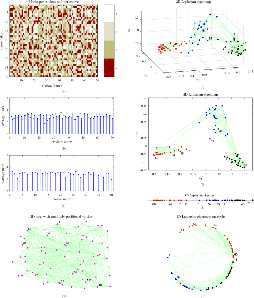
The average marks per student and per course are shown in Fig. 30(b) and 30(b)(c). Observe that average marks cannot be used to determine a student affinities.
We can now create graph by connecting with edges students with similar marks. In our example, the edge weights were determined through a distance in the -dimensional feature (marks) space, as
With the so obtained connectivity, the graph presented in Fig. 30(d), whereby the vertices (students) are randomly positioned in a plane and connected with edges. We shall now calculate normalized Laplacian eigenvectors and remap vertices according to three-dimensional, two-dimensional and one-dimensional spectral vectors defined by (67) that is, , , and . In this way, the original vertex dimensionality is reduced from to a much lower . The corresponding graph representations are respectively given in Figs. 30(e), (f), and (g). For and we can divide students into three affinity groups (marked with vertex colors). Although the obtained groups are logically ordered even in the one-dimensional case in 30(g), we cannot use for precise grouping since there is no enough gap between groups. However, even in this case, if we put vertices on circle instead on a line (by connecting two ends of a line), and draw connecting edges (the same edges as in Figs. 30(d), (e) and (f)) we can see the benefit of a graph representation even after such a radical dimensionality reduction.
The dimensionality reduction principle can also be demonstrated based on Example 4.3.3, whereby each vertex is a color image which can be represented as a vector in dimensional space. Indeed, using spectral vectors with , this graph can be presented in a two-dimensional space as in Fig. 25.
Within the Laplacian eigenmaps method, we may use any of the presented three forms of graph Laplacian eigenvectors introduced in Section 4.2.3. Relation among these three presentations is explained in Section 4.2.3 and Table 1. A unified algorithm for all three variants of the Laplacian eigenmaps, and corresponding clustering methods, is given in Algorithm 3 in the Appendix.
Remark 32: The Laplacian eigenmaps are optimal in the sense that they minimize an objective function which penalizes for the distance between the neighboring vertices in the spectral space. This ensures that if the vertices at the positions and in the original high-dimensional -dimensional spectral space are “close” in some data association metric, then they will also be close in the Euclidean sense in the reduced -dimensional space, where these positions are defined by the corresponding spectral vectors, and .
4.4.1 Euclidean distances in the space of spectral vectors.
We shall prove the “distance preserving” property of this mapping in an inductive way. Assume that a graph is connected, i.e., . The derivation is based on the quadratic form in (45)
which states that is equal to the weighted sum of squared Euclidean distances between elements of the -th and -th eigenvector at vertices and , for all and . Recall that is also equal to , by definition (see the elaboration after (43)).
Single-dimensional case. To reduce the original -dimensional vertex space to a single-dimensional path graph with vertex coordinates , the minimum sum of the weighted squared distances between the vertices and , that is
will be obtained with the new positions of vertices, designated by , with , since is the smallest nonzero eigenvalue.
Two-dimensional case. If we desire to reduce the -dimensional vertex space to a two-dimensional space, designated by and defined through any two eigenvectors of the graph Laplacian, and , then the minimum sum of the weighted squared distances between all vertices, and , given by
| (68) |
will be obtained with the new positions, , such that , since
| (69) |
for nonzero and , and having in mind that . The same reasoning holds for three- and higher-dimensional new representation spaces for the vertices, which yields (67) as optimal vertex positions in the reduced -dimensional vertex space.
The same relations hold for both the generalized eigenvectors of the Laplacian, defined by , and the eigenvectors of the normalized Laplacian, defined by . The only difference is in their normalization conditions, and .
The relation between the eigenvectors of the normalized graph Laplacian, , and the generalized eigenvectors of the graph Laplacian, , in the form , follows from their definitions (see Remark 4.2.5). Since the elements and are obtained by multiplying the elements and by the same value, , that is, , their normalized forms are identical,
4.4.2 Examples of graph analysis in spectral space
Example 28: The graph from Fig. 2, where the vertices reside in a two-dimensional plane, is shown in Fig. 31(a), while Fig. 31(b) illustrates its reduced vertex dimensionality along a line. The positions on the line are defined by the spectral vector, , with .
(a)
(b)
Remark 33: After the vertices are reordered according to the Fiedler eigenvector, , Example 4.4.2 inspires clustering refinement through the recalculation of normalized cuts. For the set of vertices , Fig. 31(b) illustrates their ordering along a line, with the new order . Instead of using the sign of to cluster the vertices, we can recalculate the normalized cuts, , with this sequential vertex order, where and , for . The estimation of the minimum normalized cut then becomes
This method is computationally efficient since only cuts, , need to be calculated. In addition, the cuts can be calculated recursively, using the previous and the connectivity parameters (degree, , and weights, ) of vertex . Any normalized cut form presented in Section 4.1 can also be used instead of . When the Cheeger ratio, defined in (42), is used in this minimization, then a simple upper bound on the normalized cut can be obtained as [67]
| (70) |
where denotes the combinatorial (true) minimum cut, with bounds given in (55).
Example 29: We shall now revisit the graph in Fig. 24 and examine the clustering scheme based on (i) standard Laplacian eigenvectors in (Fig. 32), (ii) generalized eigenvectors of graph Laplacian (Fig. 33), and (iii) eigenvectors of the normalized Laplacian (Fig. 34). Fig. 32(b) illustrates Laplacian eigenmaps based dimensionality reduction for the graph from Fig. 24(g), with the two eigenvectors, and , serving as new vertex coordinates, and using the same vertex coloring scheme as in Fig. 24(g). While both the original and the new vertex space are two-dimensional, we can clearly see that in the new vertex space the vertices belonging to the same clusters are also spatially closer, which is both physically meaningful and exemplifies the practical value of the eigenmaps. Fig. 32(c) is similar to Fig. 32(b) but is presented using the normalized spectral space coordinates, . In Fig. 32(d) the clusters are refined using the -means algorithm, as per Remark 4.3.3. The same representations are repeated and shown in Fig. 33(a)-(d) for the representation based on the generalized eigenvectors of the graph Laplacian, obtained as a solution to . Finally, in Fig. 34(a)-(d), the Laplacian eigenmaps and clustering are produced based on the eigenvectors of the normalized graph Laplacian, . As expected, the eigenmaps obtained using the generalized Laplacian eigenvectors, in Fig. 34(b), and the eigenvectors of the normalized Laplacian, in 33(b), are different; however, they reduce to the same eigenmaps after spectral vector normalization, as shown Fig. 34(c) and Fig. 33(c). After the -means based clustering refinement was applied, in all three cases two vertices switched their initial color (cluster), as shown in Fig. 32(d), Fig. 33(d), and Fig. 34(d).
Observe that the eigenmaps obtained with the normalized forms of the generalized eigenvectors of the Laplacian and the eigenvectors of the normalized Laplacian are the same, and in this case their clustering performances are similar to those based on the eigenmaps produced with eigenvectors of the original Laplacian.
(a) (b)
(c) (d)
(a) (b)
(c) (d)
(a) (b)
(c) (d)
Remark 34: In general, an independent quantization of two smoothest eigenvectors of the graph Laplacian, and , will produce four clusters. However, that will not be the case if we analyze the graph with an almost ideal eigenvalue gap (unit value) between and . In other words, when the gap tends to , that is, and , then this case corresponds to a graph with exactly two disjoint subgraph components, with vertices belonging to the disjoint sets , , and . Without loss of generality, assume . The minimum normalized cut, is then obtained with the first indicator vector for and for . The second indicator vector will produce the next minimum normalized cut, with for and for . Following the same analysis as in the case of one indicator vector and the cut of graph into two disjoint subsets of vertices, we can immediately conclude that the two smoothest eigenvectors, and , which correspond to and , can be used to form an indicator matrix , so that the corresponding matrix of the solution (within the graph Laplacian eigenvectors space) to the minimization problem of two normalized cuts, has the form The elements of indicator vectors, , have therefore a subset-wise constant vector form, assuming exactly three different vector values that correspond to individual disjoint sets , , and .
This procedure can be generalized up to every individual vertex becoming a cluster (no clustering). To characterize independent disjoint sets we will need spectral vectors, if the constant eigenvector, , is omitted.
Example 30: The Laplacian eigenmap for the Minnesota roadmap graph in the two-dimensional case, with , is given in Fig. 35. In this new space, the spectral vectors , are used as the coordinates of new vertex positions, , . Here, two vertices with similar slow-varying eigenvectors are located close to one another in the new coordinate system defined by , . This illustrates that the eigenmaps can be considered as a basis for “scale-wise ”graph representation.
Example 31: The Laplacian eigenmaps of the Brain Atlas graph from Fig. 29, whose original vertex locations reside in an dimensional space, is presented in a new reduced dimensional space defined based on the two smoothest eigenvectors, and . This is an example of vertex dimensionality reduction. This new graph, with new vertex locations but with the original edges kept, is shown in Fig. 36.
(a)
(b)
The generalized eigenvectors of the graph Laplacian, , for , are shown in Fig. 37(a) using the standard colormap in both the original three-dimensional and the reduced two-dimensional space, as shown in Fig. 37(b).


Example 32: Vertices of a three-dimensional Swiss roll graph are shown in Fig. 39(a). The vertex locations in this dimensional space are calculated as , and , , with randomly taking values between and , and from to . The edge weights are calculated using , where is the square Euclidean distance between the vertices and , and if with . The resulting three-dimensional Swiss roll graph is shown in Fig. 39(b), while Fig. 39(c) shows the same graph but with vertices colored (clustered) using the normalized graph Laplacian eigenvectors, and , as a colormap. The same vectors are then used as the new coordinates in the reduced two-dimensional Laplacian eigenmap vertex space for the Swiss roll graph, given in Fig. 39(d).
4.5 Pseudo-inverse of Graph Laplacian-Based Mappings
The graph Laplacian is a singular matrix (since ) for which an inverse does not exist. To deal with this issue, the pseudo-inverse of the graph Laplacian, , is defined as a matrix that satisfies the property
| (71) |
The eigenvalues of the graph Laplacian pseudo-inverse are the inverses of the original eigenvalues, , while it shares the same eigenvectors with the original graph Laplacian, , , , . The eigenmaps for which the corresponding spectral coordinates are scaled based on the eigenvalues of the pseudo-inverse of graph Laplacian can be interpreted within the Principal Component Analysis (PCA) framework in the following way.
The eigenmaps based on the pseudo-inverse of the Laplacian are the same as for the original graph Laplacian since they share the same eigenvectors. If the spectral vectors are scaled with the square roots of the eigenvalues of Laplacian pseudo-inverse we obtain
The elements of the spectral vector are now equal to the first elements (omitting ) of the full-scale spectral vector
| (72) |
where is a diagonal matrix with elements
4.5.1 Commute time mapping
The physical meaning of these new positions in the spectral space is related to the notion of commute time, which is a property of a diffusion process on a graph [74, 75]. The commute time, between vertices and is defined as the expected time for the random walk to reach vertex starting from vertex , and then to return. Its is proportional to the Euclidean distance of vertices, with the positions in the new space defined by in (72), that is
where is the volume of the whole graph, .
To put this into perspective, in a graph representation of a resistive electric circuit/network, for which the edge weights are equal to the conductances (inverse resistances, see Part 3), the commute time, , is defined by the equivalent resistance between the electric circuit nodes (vertices) and [76].
The covariance matrix of the scaled spectral vectors is given by
In other words, the reduced dimensionality space of eigenvectors, , , , , is the space of which the principal directions correspond to the maximum variance of the graph embedding, since , which in turn directly corresponds to principal component analysis (PCA).
Remark 35: Two-dimensional case comparison. The two-dimensional spectral space of the standard graph Laplacian eigenvectors is defined by and , while the spectral vector in this space is given by
In the case of commute time mapping, the two-dimensional spectral domain of the vertices is defined as
| (73) |
The commute time mapping is related to the graph Laplacian mapping through an appropriate axis scaling.
We can conclude that when these two mappings are almost the same, when normalized.
However, when , the relative eigenvalue gap between the one dimensional and two-dimensional spectral space is large, since is close to . This means that the segmentation into two disjoint subgraphs will be close to the original graph, while at the same time this also indicates that the eigenvector does not contribute to a new close segmentation (in the sense of Section 4.3.2), since its gap is not small. Therefore, the influence of should be reduced, as compared to the standard graph Laplacian spectral vector where both and are used with equal unity weight, . This reduction of the influence of the irrelevant vector , when , is exactly what is achieved in the commute time mapping, since .
For the graph from Example 4.4.2, shown in Fig. 32(a), the commute time mapping will produce the same presentation as in Fig. 32(b), which is obtained with the eigenvectors of the graph Laplacian, when the vertical, , axis is scaled by
This eigenmap will be very close to the eigenmap in Fig. 32(b), produced based on the graph Laplacian eigenvectors and spectral vector .
4.5.2 Diffusion (Random Walk) Mapping
Finally, we shall now relate the commute time mapping to the diffusion mapping.
Definition: Diffusion on a graph deals with the problem of propagation along the edges of a graph, whereby at the initial step, , the random walk starts at a vertex . At the next step , the walker moves from its current vertex to one of its neighbors , chosen uniformly at random from the neighbors of . The probability of going from vertex to vertex is equal to the ratio of the weight and the sum of all possible edge weights from the vertex , that is
| (74) |
When considering all vertices together, such probabilities can be written in a matrix form, within the weight of a random walk matrix, defined as in (13), by
| (75) |
Diffusion distance. The diffusion distance between the vertices and , denoted by , is equal to the distance between the vector (-dimensional ordered set) of probabilities for a random walk to move from a vertex to all other vertices (as in (74)), given by
and the corresponding vector of probabilities for a random walk to move from a vertex to all other vertices, given by
that is
where is constant for a given graph, and is equal to the sum of degrees (volume) of all graph vertices in .
Example 33: For the graph from Fig. 2, with its weight matrix, , and the degree matrix, , given respectively in (7) and (9), the random walk weight matrix in (75) is of the form
| (76) |
with .
Therefore, the diffusion distance between, for example, the vertices and , for the step, is
while the diffusion distance between the vertices and is . From this simple example, we can see that the diffusion distance is larger for vertices and than for the neighboring vertices and . This result is in a perfect accordance with the clustering scheme (expected similarity) in Fig. 23(b), where the vertices and are grouped into the same cluster, while the vertices and belong to different clusters.
The probability vectors are called the diffusion clouds (in this case for step ), since they resemble a cloud around a vertex . The diffusion distance can then be considered as a distance between the diffusion clouds (sets of data) around a vertex and a vertex . If the vertices are well connected (approaching a complete graph structure) then this distance is small, while for vertices with long paths between them, this distance is large.
The diffusion analysis can be easily generalized to any value of the diffusion step, , whereby after steps, the matrix of probabilities in (75) becomes
The elements of this matrix, denoted by , are equal to the probabilities that a random walker moves from a vertex to a vertex , in steps. The -step diffusion distance between the vertices and , is accordingly defined as
where
and
It can be shown that the diffusion distance is equal to the Euclidean distance between the considered vertices when they are presented in a new space of their generalized Laplacian eigenvectors, which are then scaled by their corresponding eigenvalues; this new space is referred to as the diffusion maps (cf. eigenmaps).
The eigenanalysis relation for the random walk weight matrix for the state now becomes
Since the weight matrix can be written as , this yields , or
to finally produce the generalized graph Laplacian equation,
with . This relation indicates that a one-step diffusion mapping is directly obtained from the corresponding generalized graph Laplacian mapping.
After steps, the random walk matrix (of probabilities) becomes
for which the eigenvalues are , while the (right) eigenvectors remain the same as for the graph Laplacian, see (31).
The spectral space for vertices, for a -step diffusion process (diffusion mapping), is then defined based on the spectral vector
and is equal to the generalized Laplacian spectral space mapping, whereby the axis vectors are multiplied by the corresponding eigenvalues, .
It can be shown that the diffusion distance between vertices in the new diffusion map space is equal to their Euclidean distance [77], that is
| (77) |
Example 34: For the graph from Fig. 2, whose weight matrix, , and the degree matrix, , are defined in (7) and (9), the diffusion distance between the vertices and can be calculated using (77) as
where the spectral vectors, and are obtained using the generalized graph Laplacian eigenvectors, , and the corresponding eigenvalues, , from . This is the same diffusion distance value, , as in Example 4.5.2.
Dimensionality reduced diffusion maps. Dimensionality of the vertex representation space can be reduced in diffusion maps by keeping only the eigenvectors that correspond to the most significant eigenvalues, , , in the same way as for the Laplacian eigenmaps,
For example, the two-dimensional spectral domain of the vertices in the diffusion mapping is defined as
while the analysis and intuition for the diffusion mapping is similar to that for the commute time mapping, presented in Remark 4.5.1, diffusion maps have an additional degree of freedom, the step .
Example 35: For the graph in Fig 25, which corresponds to a set of real-world images, the commute time two-dimensional spectral vectors in (73), normalized by the first eigenvector value through a multiplication of its coordinates by , assume the form
The corresponding vertex colors indicate diffusion-based clustering, as shown in Fig. 40(a). Fig. 40(b) shows the vertices of this graph, colored with the two-dimensional diffusion map spectral vectors, normalized by , to yield
(a)(b)
Finally, the sum over all steps, , of the diffusion space yields
since the sum of a geometric progression is equal to
This mapping also corresponds to the cumulative diffusion distance, given by
The diffusion eigenmaps can be therefore obtained by appropriate axis scaling of the standard eigenmaps, produced by the generalized eigenvectors of the graph Laplacian.
Remark 36: The commute time and the diffusion process mappings are related in the same way as the mappings based on the graph Laplacian eigenvectors and the generalized eigenvectors of the graph Laplacian.
4.6 Summary of Embedding Mappings
| Mapping | Eigen-analysis relation | Reduced dimensionality spectral vector |
|---|---|---|
| Graph Laplacian mapping | ||
| Generalized eigenvectors | ||
| of Laplacian mapping | ||
| Normalized Laplacian mapping | ||
| Commute time mapping | ||
| Diffusion (random walk) mapping | ||
| Cumulative diffusion mapping |
A summary of the embedding mappings considered is given in Table 1. Various normalization schemes may be used to obtain the axis vectors, , from the spectral vectors, , for the presentation (see Algorithm 3).
These examples of dimensionality reduction reveal close connections with spectral clustering algorithms developed in standard machine learning and computer vision; in this sense, the notions of dimensionality reduction and clustering can be considered as two sides of the same coin [65]. In addition to the reduction of dimensionality for visualization purposes, the resulting vertex space of lower dimensionality may be used to mitigate the complexity and accuracy issues experienced with classification algorithms, or in other words to bypass the course of dimensionality.
5 Graph Sampling Strategies
In the case of extremely large graphs, subsampling and down-scaling of graphs is a prerequisite for their analysis [78]. For a given large (in general directed) graph, , with vertices, the resampling aims to find a much simpler graph which retains most of the properties of the original graph, and is both less complex and more physically and computationally meaningful. The similarity between the original large graph , and the down-scaled graph, , with vertices, where , is defined with respect to the set of parameters of interest, like for example, the connectivity or distribution on a graph. Such criteria may also be related to the spectral behavior of graphs.
Several methods exist for graph down-scaling, some of which are listed below.
- •
The simplest method for graph down-sampling is the random vertex or random node (RN) selection method, whereby a random subset of vertices is used for the analysis and representation of large graphs and data observed on such large graphs. Even though the vertices are selected with equal probabilities, this method produces good results in practical applications.
- •
Different from the RN method, where the vertices are selected with a uniform probability, the random degree vertex/node (RDN) selection method is based on the probability of vertex selection that is proportional to the vertex degree. In other words, vertices with more connections, thus having larger , are selected with higher probability. This makes the RDN approach biased with respect to highly connected vertices.
- •
The PageRank method is similar to the RDN, and is based on the vertex rank. The PageRank is defined by the importance of the vertices connected to the considered vertex . Then, the probability that a vertex will be used in a down-scaled graph is proportional to the PageRank of this vertex. This method is also known as the random PageRank vertex (RPN) selection, and is biased with respect to the highly connected vertices (with a high PageRank).
- •
A method based on a random selection of edges that will remain in the simplified graph is called the random edge (RE) method. This method may lead to graphs that are not well connected, and which exhibit large diameters.
- •
The RE method may be combined with random vertex selection to yield a combined RNE method, whereby a random vertex selection is followed by a random selection of one of the edges corresponding to the selected vertex.
- •
In addition to these methods, more sophisticated methods based on random vertex selection and random walk (RW) analysis may be defined. For example, we can randomly select a small subset of vertices and form several random walks starting from each selected vertex. The Random Walk (RW), Random Jump (RJ) and Forest Fire graph down-scaling strategies are all defined in this way.
6 Conclusion
Although within the graph data analytics paradigm, graphs have been present in various forms for centuries, the advantages of a graph framework for data analytics on graphs, as opposed to the optimization of the graphs themselves, have been recognized rather recently. In order to provide a comprehensive and Data Analytics friendly introduction to graph signal processing, an overview of graphs from this specific practitioner-friendly signal processing point of view is a prerequisite.
In this part of our article, we have introduced graphs as irregular signal domains, together with their properties relevant for data analytics applications which rest upon the estimation of signals on graphs. This has been achieved in a systematic and example rich way and by highlighting links with classic matrix analysis and linear algebra. Spectral analysis of graphs has been elaborated upon in detail, as this is a main underpinning methodology for efficient data analysis, the ultimate goal in Data Science. Both the adjacency matrix and the Laplacian matrix have been used in this context, along with their spectral decompositions. Finally, we have highlighted important aspects of graph segmentation and Laplacian eigenmaps, and have emphasized their role as the foundation for advances in Data Analytics on graphs.
Part 2 will address theory and methods of processing data on graphs, while Part 3 is devoted to unsupervised graph topology learning, from the observed data.
7 Appendix: Power Method for Eigenanalysis
Computational complexity of the eigenvalue and eigenvector calculation for a symmetric matrix is of the order of , which is computationally prohibitive for very large graphs, especially when only a few the smoothest eigenvectors are needed, like in spectral graph clustering. To mitigate this computational bottleneck, an efficient iterative approach, called the Power Method, may be employed.
Consider the normalized weight matrix,
and assume that the eigenvalues of are , with the corresponding eigenvectors, . Consider an arbitrary linear combination of the eigenvectors, , through the coefficients ,
Further multiplication of the vector by the normalized weight matrix, , results in
A repetition of this multiplication times yields
In other words, we have just calculated the first eigenvector of , given by
through only matrix products of and [67, 79]. Convergence of this procedure depends on and requires that is not close to . Note that is a highly sparse matrix, which significantly reduces the calculation complexity.
After the eigenvector is obtained, the corresponding eigenvalue can be calculated as its smoothing index, .
After and are calculated, we can remove their contribution from the normalized weight matrix, through deflation, as , and then continue to calculate the next largest eigenvalue and its eigenvector, and . The procedure can be repeated iteratively until the desired number of eigenvectors is found.
The relation of the normalized weight matrix, , with the normalized graph Laplacian, , is given by
while the relation between the eigenvalues and eigenvectors of and follows from , to yield
The eigenvalues of and are therefore related as , and share the same corresponding eigenvectors, , of the normalized graph Laplacian and the normalized weight matrix. This means that corresponds to and that the second largest eigenvalue of produces the Fiedler vector of the normalized Laplacian.
Note that the second largest eigenvector of is not necessarily since the eigenvalues of can be negative.
Example 36: The weight matrix from (7) is normalized by the degree matrix from (9) to arrive at . The power algorithm is then used to calculate the four largest eigenvalues and the corresponding eigenvectors of in 200 iterations, to give . These are very close to the four exact largest eigenvalues of , . Note that the Fiedler vector of the normalized graph Laplacian is associated with as it corresponds to the second largest eigenvalue of , when the eigenvalue signs are accounted for. Even when calculated using the approximative power method, the Fiedler vector is close to its exact value, as shown in Fig. 22(d), with the maximum relative error of its elements being .
Notice that it is possible to calculate the Fiedler vector of a graph Laplacian even without using the weight matrix. Consider a graph whose eigenvalues of the Laplacian are , where corresponds to the largest value of the sequence . These are also the eigenvalues of the pseudo-inverse of the graph Laplacian, . Now, since the pseudo-inverse of the graph Laplacian, , and the graph Laplacian, , have the same eigenvectors, we may also apply the power method to the pseudo-inverse of the graph Laplacian, , and the eigenvector corresponding to the largest eigenvalue is the Fiedler vector.
- •
Normalized weight matrix
- •
Number of iterations,
- •
Number of the desired largest eigenvectors,
- •
Largest eigenvalues and the corresponding eigenvectors
- •
Fiedler vector of the normalized graph Laplacian is the eigenvector of the second largest eigenvalue, , .
8 Appendix: Algorithm for Graph Laplacian Eigenmaps
The algorithm for the Laplacian eigenmap and spectral clustering based on the eigenvectors of the graph Laplacian, the generalized eigenvectors of the graph Laplacian, and the eigenvectors of the normalized Laplacian, is given in the pseudo-code form in Algorithm 3.
- •
Vertex positions, rows of
- •
Weight matrix , with elements
- •
Laplacian eigenmap dimensionality,
- •
Position, mapping, normalization, and coloring indicators
- •
New graph
- •
Subsets of vertex clusters
References
References
- [1] N. Christofides, Graph theory: An algorithmic approach, Academic Press, 1975.
- [2] F. Afrati, A. G. Constantinides, The use of graph theory in binary block code construction, in: Proceedings of the International Conference on Digital Signal Processing, 1978, pp. 228–233.
- [3] O. J. Morris, M. d. J. Lee, A. G. Constantinides, Graph theory for image analysis: An approach based on the shortest spanning tree, IEE Proceedings F-Communications, Radar and Signal Processing 133 (2) (1986) 146–152.
- [4] L. J. Grady, J. R. Polimeni, Discrete calculus: Applied analysis on graphs for computational science, Springer Science & Business Media, 2010.
- [5] S. S. Ray, Graph theory with algorithms and its applications: in Applied Science and Technology, Springer Science & Business Media, 2012.
- [6] A. Marques, A. Ribeiro, S. Segarra, Graph signal processing: Fundamentals and applications to diffusion processes, in: Proc. Int. Conf. Accoustic, Speech and Signal Processing, (ICASSP), 2017, IEEE, 2017.
- [7] H. Krim, A. B. Hamza, Geometric methods in signal and image analysis, Cambridge University Press, 2015.
- [8] M. I. Jordan, Learning in graphical models, Vol. 89, Springer Science & Business Media, 1998.
- [9] A. Bunse-Gerstner, W. B. Gragg, Singular value decompositions of complex symmetric matrices, Journal of Computational and Applied Mathematics 21 (1) (1988) 41–54.
- [10] D. S. Grebenkov, B.-T. Nguyen, Geometrical structure of Laplacian eigenfunctions, SIAM Review 55 (4) (2013) 601–667.
- [11] R. Bapat, The Laplacian matrix of a graph, Mathematics Student-India 65 (1) (1996) 214–223.
- [12] S. O’Rourke, V. Vu, K. Wang, Eigenvectors of random matrices: A survey, Journal of Combinatorial Theory, Series A 144 (2016) 361–442.
- [13] K. Fujiwara, Eigenvalues of Laplacians on a closed Riemannian manifold and its nets, Proceedings of the American Mathematical Society 123 (8) (1995) 2585–2594.
- [14] S. U. Maheswari, B. Maheswari, Some properties of Cartesian product graphs of Cayley graphs with arithmetic graphs, International Journal of Computer Applications 138 (3) (2016) 26–29.
- [15] M. I. Jordan, et al., Graphical models, Statistical Science 19 (1) (2004) 140–155.
- [16] J. M. Moura, Graph signal processing, in: Cooperative and Graph Signal Processing, P. Djuric and C. Richard, Editors, Elsevier, 2018, pp. 239–259.
- [17] M. Vetterli, J. Kovačević, V. Goyal, Foundations of signal processing, Cambridge University Press., 2014.
- [18] A. Sandryhaila, J. M. Moura, Discrete signal processing on graphs, IEEE Transactions on Signal Processing 61 (7) (2013) 1644–1656.
- [19] V. N. Ekambaram, Graph-structured data viewed through a Fourier lens, University of California, Berkeley, 2014.
- [20] A. Sandryhaila, J. M. Moura, Discrete signal processing on graphs: Frequency analysis, IEEE Transactions on Signal Processing 62 (12) (2014) 3042–3054.
- [21] A. Sandryhaila, J. M. Moura, Big data analysis with signal processing on graphs: Representation and processing of massive data sets with irregular structure, IEEE Signal Processing Magazine 31 (5) (2014) 80–90.
- [22] D. I. Shuman, S. K. Narang, P. Frossard, A. Ortega, P. Vandergheynst, The emerging field of signal processing on graphs: Extending high-dimensional data analysis to networks and other irregular domains, IEEE Signal Processing Magazine 30 (3) (2013) 83–98.
- [23] R. Hamon, P. Borgnat, P. Flandrin, C. Robardet, Extraction of temporal network structures from graph-based signals, IEEE Transactions on Signal and Information Processing over Networks 2 (2) (2016) 215–226.
- [24] S. Chen, A. Sandryhaila, J. M. Moura, J. Kovačević, Signal denoising on graphs via graph filtering, in: Proc. 2014 IEEE Global Conference on Signal and Information Processing (GlobalSIP), 2014, pp. 872–876.
- [25] A. Gavili, X.-P. Zhang, On the shift operator, graph frequency, and optimal filtering in graph signal processing, IEEE Transactions on Signal Processing 65 (23) (2017) 6303–6318.
- [26] M. J. Wainwright, M. I. Jordan, et al., Graphical models, exponential families, and variational inference, Foundations and Trends® in Machine Learning 1 (1–2) (2008) 1–305.
- [27] D. M. Cvetković, M. Doob, H. Sachs, Spectra of graphs: Theory and application, Vol. 87, Academic Press, 1980.
- [28] D. M. Cvetković, M. Doob, Developments in the theory of graph spectra, Linear and Multilinear Algebra 18 (2) (1985) 153–181.
- [29] D. M. Cvetković, I. Gutman, Selected topics on applications of graph spectra, Matematički Institut SANU (Serbian Academy of Scences and Arts), 2011.
- [30] A. E. Brouwer, W. H. Haemers, Spectra of graphs, Springer-Verlag New York, 2012.
- [31] F. Chung, Spectral graph theory, AMS, Providence, RI, 1997.
- [32] O. Jones, Spectra of simple graphs[Online]. Available: https://www.whitman.edu/Documents/Academics /Mathematics/Jones.pdf, Whitman College, 2013.
- [33] D. Mejia, O. Ruiz-Salguero, C. A. Cadavid, Spectral-based mesh segmentation, International Journal on Interactive Design and Manufacturing (IJIDeM) 11 (3) (2017) 503–514.
- [34] L. Stanković, E. Sejdić, M. Daković, Vertex-frequency energy distributions, IEEE Signal Processing Letters.
- [35] L. Stanković, M. Daković, E. Sejdić, Vertex-frequency energy distributions, in: Vertex-Frequency Analysis of Graph Signals, Springer, 2019, pp. 377–415.
- [36] H. Lu, Z. Fu, X. Shu, Non-negative and sparse spectral clustering, Pattern Recognition 47 (1) (2014) 418–426.
- [37] X. Dong, P. Frossard, P. Vandergheynst, N. Nefedov, Clustering with multi-layer graphs: A spectral perspective, IEEE Transactions on Signal Processing 60 (11) (2012) 5820–5831.
- [38] R. Horaud, A short tutorial on graph Laplacians, Laplacian embedding, and spectral clustering, [Online], Available: http://csustan.csustan.edu/ tom/Lecture-Notes/Clustering/GraphLaplacian-tutorial.pdf (2009).
- [39] R. Hamon, P. Borgnat, P. Flandrin, C. Robardet, Relabelling vertices according to the network structure by minimizing the cyclic bandwidth sum, Journal of Complex Networks 4 (4) (2016) 534–560.
- [40] M. Masoumi, A. B. Hamza, Spectral shape classification: A deep learning approach, Journal of Visual Communication and Image Representation 43 (2017) 198–211.
- [41] M. Masoumi, C. Li, A. B. Hamza, A spectral graph wavelet approach for nonrigid 3D shape retrieval, Pattern Recognition Letters 83 (2016) 339–348.
- [42] L. Stanković, M. Daković, E. Sejdić, Vertex-frequency analysis: A way to localize graph spectral components [lecture notes], IEEE Signal Processing Magazine 34 (4) (2017) 176–182.
- [43] L. Stanković, E. Sejdić, M. Daković, Reduced interference vertex-frequency distributions, IEEE Signal Processing Letters.
- [44] L. Stankovic, D. Mandic, M. Dakovic, I. Kisil, E. Sejdic, A. G. Constantinides, Understanding the basis of graph signal processing via an intuitive example-driven approach, IEEE Signal Processing Magazine (2019) submitted.
- [45] F. R. Chung, R. P. Langlands, A combinatorial laplacian with vertex weights, journal of combinatorial theory, Series A 75 (2) (1996) 316–327.
- [46] A. Duncan, Powers of the adjacency matrix and the walk matrix, The Collection (2004) 1–11.
- [47] S. Saito, D. P. Mandic, H. Suzuki, Hypergraph p-Laplacian: A differential geometry view, in: Thirty-Second AAAI Conference on Artificial Intelligence, 2018.
- [48] E. R. Van Dam, W. H. Haemers, Which graphs are determined by their spectrum?, Linear Algebra and Its Applications 373 (2003) 241–272.
- [49] S. E. Schaeffer, Graph clustering, Computer Science Review 1 (1) (2007) 27–64.
- [50] J. N. Mordeson, P. S. Nair, Fuzzy graphs and fuzzy hypergraphs, Vol. 46, Physica, 2012.
- [51] J. Kleinberg, E. Tardos, Algorithm design, Pearson Education India, 2006.
- [52] O. Morris, M. d. J. Lee, A. Constantinides, Graph theory for image analysis: An approach based on the shortest spanning tree, IEE Proceedings F (Communications, Radar and Signal Processing) 133 (2) (1986) 146–152.
- [53] S. Khuller, Approximation algorithms for finding highly connected subgraphs, Tech. rep. (1998).
- [54] A. K. Jain, Data clustering: 50 years beyond k-means, Pattern Recognition Letters 31 (8) (2010) 651–666.
- [55] I. S. Dhillon, Y. Guan, B. Kulis, Kernel k-means: Spectral clustering and normalized cuts, in: Proceedings of the Tenth ACM SIGKDD International Conference on Knowledge Discovery and Data Mining, ACM, 2004, pp. 551–556.
- [56] M. Stoer, F. Wagner, A simple min-cut algorithm, Journal of the ACM (JACM) 44 (4) (1997) 585–591.
- [57] G. Kron, Diakoptics: the piecewise solution of large-scale systems, Vol. 2, MacDonald, 1963.
- [58] L. Hagen, A. B. Kahng, New spectral methods for ratio cut partitioning and clustering, IEEE transactions on computer-aided design of integrated circuits and systems 11 (9) (1992) 1074–1085.
- [59] J. Shi, J. Malik, Normalized cuts and image segmentation, Departmental Papers (CIS) (2000) 107.
- [60] B. Mohar, Isoperimetric numbers of graphs, Journal of combinatorial theory, Series B 47 (3) (1989) 274–291.
- [61] M. Fiedler, Algebraic connectivity of graphs, Czechoslovak mathematical journal 23 (2) (1973) 298–305.
- [62] J. Malik, S. Belongie, T. Leung, J. Shi, Contour and texture analysis for image segmentation, International Journal of Computer Vision 43 (1) (2001) 7–27.
- [63] A. Y. Ng, M. I. Jordan, Y. Weiss, On spectral clustering: Analysis and an algorithm, in: Proc. Advances in Neural Information Processing Systems, 2002, pp. 849–856.
- [64] D. A. Spielman, S.-H. Teng, Spectral partitioning works: Planar graphs and finite element meshes, Linear Algebra and its Applications 421 (2-3) (2007) 284–305.
- [65] M. Belkin, P. Niyogi, Laplacian eigenmaps for dimensionality reduction and data representation, Neural Computation 15 (6) (2003) 1373–1396.
- [66] F. Chung, Laplacians and the cheeger inequality for directed graphs, Annals of Combinatorics 9 (1) (2005) 1–19.
- [67] L. Trevisan, Lecture notes on expansion, sparsest cut, and spectral graph theory (2013).
- [68] Y. Weiss, Segmentation using eigenvectors: A unifying view, in: Proceedings of the Seventh IEEE International Conference on Computer Vision, Vol. 2, IEEE, 1999, pp. 975–982.
- [69] P. Perona, W. Freeman, A factorization approach to grouping, in: Prof. of European Conference on Computer Vision, Springer, 1998, pp. 655–670.
- [70] G. L. Scott, H. C. Longuet-Higgins, Feature grouping by relocalisation of eigenvectors of the proximity matrix., in: Proc. of the British Machine Vision Conference (BMVC), 1990, pp. 1–6.
- [71] Z. Wang, E. P. Simoncelli, A. C. Bovik, Multiscale structural similarity for image quality assessment, in: Proc. of The Thrity-Seventh Asilomar Conference on Signals, Systems & Computers, 2003, Vol. 2, 2003, pp. 1398–1402.
- [72] M. Mijalkov, E. Kakaei, J. B. Pereira, E. Westman, G. Volpe, BRAPH: A graph theory software for the analysis of brain connectivity, PLOS ONE 12.8 (2017): e0178798doi:https://doi.org/10.1371/journal.pone.0178798.
- [73] M. Rubinov, O. Sporns, Complex network measures of brain connectivity: Uses and interpretations, NeuroImage 52 (3) (2010) 1059 – 1069, computational Models of the Brain. doi:https://doi.org/10.1016/j.neuroimage.2009.10.003.
- [74] H. Qiu, E. R. Hancock, Clustering and embedding using commute times, IEEE Transactions on Pattern Analysis and Machine Intelligence 29 (11) (2007) 1873–1890.
- [75] R. Horaud, A short tutorial on graph Laplacians, Laplacian embedding, and spectral clustering (2012).
- [76] A. K. Chandra, P. Raghavan, W. L. Ruzzo, R. Smolensky, P. Tiwari, The electrical resistance of a graph captures its commute and cover times, Computational Complexity 6 (4) (1996) 312–340.
- [77] R. R. Coifman, S. Lafon, Diffusion maps, Applied and computational harmonic analysis 21 (1) (2006) 5–30.
- [78] J. Leskovec, C. Faloutsos, Sampling from large graphs, in: Proceedings of the 12th ACM SIGKDD International Conference on Knowledge Discovery and Data Mining, ACM, 2006, pp. 631–636.
- [79] M. Tammen, I. Kodrasi, S. Doclo, Complexity reduction of eigenvalue decomposition-based diffuse power spectral density estimators using the power method, in: Proc. of the IEEE International Conference on Acoustics, Speech and Signal Processing (ICASSP), IEEE, 2018, pp. 451–455.