Deep splitting method for parabolic PDEs
Abstract
In this paper we introduce a numerical method for nonlinear parabolic PDEs that combines operator
splitting with deep learning. It divides the PDE approximation problem into a sequence of separate learning
problems. Since the computational graph for each of the subproblems is comparatively small, the approach
can handle extremely high-dimensional PDEs. We test the method on different examples from physics,
stochastic control and mathematical finance. In all cases, it yields very good results in up to 10,000
dimensions with short run times.
Key words. nonlinear partial differential equations, splitting-up method,
neural networks, deep learning
AMS subject classifications. 35K15, 65C05, 65M22, 65M75, 91G20, 93E20
1 Introduction
In this paper we derive a numerical scheme for parabolic partial differential equations (PDEs) of the form
| (1.1) |
, with initial condition , where , , and are appropriate continuous functions. Such PDEs describe various phenomena in nature, engineering, economics, and finance. They typically do not admit closed form solutions and, therefore, have to be solved numerically. In some applications, the dimension can be high. For instance, in physics and engineering applications, typically models the coordinates of all components of a given system, whereas in derivative pricing and optimal investment problems, usually corresponds to the number of underlying assets. Many classical PDEs, such as the standard heat and Black–Scholes equations are linear. Using the Feynman–Kac representation, their solutions can efficiently be approximated in high dimensions with simple Monte Carlo averages. But if constraints or frictions are taken into account, or the PDE describes a control problem, the function is no longer linear and equation (1.1) becomes much more challenging to solve for large .
Numerical methods for PDEs have a long history. Classical approaches like finite differences and finite elements (see, e.g., [13, 71, 95]) are deterministic. In their standard form, they work well for and , but their complexity grows exponentially in . To tackle higher dimensional problems, different simulation-based approaches have been developed that exploit a stochastic representation of the solution of the PDE. For instance, [1, 7, 8, 12, 15, 16, 17, 18, 19, 20, 21, 22, 24, 26, 36, 37, 38, 39, 40, 41, 54, 70, 73, 74, 77, 78, 79, 84, 85, 87, 89, 90, 91, 96, 98] use BSDE representations of PDEs and study approximation methods based on recursive polynomial regressions, [50, 52, 53, 82, 93, 97] investigate methods based on branching diffusion processes, and [29, 30, 57, 59, 60] analyze full-history recursive multilevel Picard methods. Recently, numerical methods for high-dimensional PDEs based on the idea to reformulate the PDE as a stochastic learning problem have been proposed in [28, 48]. This opens the door to the application of deep learning; see, e.g., [2, 3, 6, 10, 14, 31, 33, 34, 42, 49, 51, 55, 62, 75, 76, 80, 88, 92] for modifications and extensions. There are also already a few papers studying the convergence of deep learning based approximation methods for PDEs. For instance, [49, 92] derive convergence results without information on the convergence speed, whereas [11, 32, 44, 56, 63, 69] provide convergence and tractability results with dimension-independent convergence rates and error constants depending polynomially on the dimension.
In this paper we develop a new deep learning method for parabolic PDEs that splits the differential operator into a linear and a nonlinear part. More precisely, we write
| (1.2) |
for suitable continuous functions and . This decomposition is not unique. But the idea is that is chosen such that the nonlinearity becomes small. Then we solve the PDE iteratively over small time intervals by approximating and using the Feynman–Kac representation locally. This requires a recursive computation of conditional expectations. We approximate them by formulating them as minimization problems that can be approached with deep learning. This decomposes the PDE approximation problem into a sequence of separate learning problems. Since the computational graph for each of the subproblems is comparatively small, the method works for very high-dimensional problems.
The rest of the paper is organized as follows. In Section 2 we introduce the framework and derive the deep splitting method. In Section 3 we test the approach on five different classes of high-dimensional nonlinear PDEs: Hamilton–Jacobi–Bellman (HJB) equations, nonlinear Black–Scholes equations, Allen–Cahn-type equations, nonlinear heat equations, and sine-Gordon-type equations.
2 Derivation of the proposed approximation algorithm
Fix and . Consider two at most polynomially growing continuous functions and together with two Lipschitz continuous functions and . Assume is an at most polynomially growing continuous function that is on and satisfies the PDE
| (2.1) |
, with initial condition , .
2.1 Temporal discretization
To approximate the solution of the PDE (2.1), we discretize the equation in time and use a splitting-up method (see, e.g., [43, 45, 46]) to obtain a semi-discrete approximation problem. To do this, we choose and let be real numbers such that
| (2.2) |
Under appropriate integrability assumptions, it follows from (2.1) that for every , we have
| (2.3) |
In particular, for all , and ,
| (2.4) |
and therefore,
| (2.5) |
which can be written as
| (2.6) |
To derive the splitting-up approximation, we make a few simplifying assumptions, not all of which are needed to implement the resulting algorithm. First, we suppose that has an at most polynomially growing gradient . Moreover, we assume that there exists a function satisfying , , such that for every , belongs to with at most polynomially growing partial derivatives and for all , and ,
| (2.7) |
see, e.g., Hairer et al. [47, Section 4.4], Deck & Kruse [23], Krylov [67, Chapter 8], and Krylov [68, Theorem 4.32] for existence, uniqueness, and regularity results for equations of the form (2.7). Comparing (2.7) to (2.6) suggests that
| (2.8) |
So is a specific splitting-up type approximation of the function ; see, e.g., [25, 43, 45, 46].
2.2 An approximate Feynman–Kac representation
In the next step we derive a Feynman–Kac representation of ; see, e.g., Milstein & Tretyakov [86, Section 2]. Let be a standard -Brownian motion on a filtered probability space satisfying the usual conditions. Consider an /-measurable random variable satisfying for every , and let be an -adapted process with continuous sample paths satisfying for every ,
| (2.9) |
The assumption that for all ensures that
| (2.10) |
see, e.g., Stroock [94, Section 1.2]. Moreover, (2.7) implies that for all , and , one has
| (2.11) |
from which it follows that for all , and ,
| (2.12) |
Since for every , is in , we obtain from Itô’s formula that for all and we have
| (2.13) |
which by (2.12), gives that -a.s.,
| (2.14) |
Moreover, since, by assumption, is Lipschitz continuous and at most polynomially growing in , one obtains from (2.10) that for all and ,
| (2.15) |
from which it follows that
| (2.16) |
Together with (2.14), this shows that for all and we have
| (2.17) |
Since is /-measurable, one obtains from the tower property of conditional expectations that for all and ,
| (2.18) |
Since has continuous sample paths and at most polynomially growing first order partial derivatives, it follows from (2.7) and (2.11) that we have for all and ,
| (2.19) |
In addition, since for every , we obtain
| (2.20) |
So it follows from (2.18) and (2.19) that for all ,
| (2.21) |
which is the Feynman–Kac type representation we were aiming for. Note that the nonlinearity as well as the coefficient functions and in (2.1) do not depend on . But the above derivation could be extended to time-dependent , , and since the Feynman–Kac formula still holds in this case.
2.3 Formulation as recursive minimization problems
We now reformulate (2.21) as recursive minimization problems. It follows from our assumptions that for every , is at most polynomially growing in . Therefore, we obtain from (2.10) that
| (2.22) |
Since is continuous in , it follows from the factorization lemma and the -minimality property of conditional expectations (see, e.g., Klenke [65, Corollary 8.17]) that for every we have
| (2.23) |
2.4 Deep artificial neural network approximations
To tackle the minimization problems (2.23) numerically, we approximate the functions , , with neural networks . More precisely, we choose and . Then, we set and consider functions , , such that for every , is given by
| (2.24) |
and for , is of the form
| (2.25) |
where for and with is the affine function defined by
| (2.26) |
and is a mapping of the form
| (2.27) |
for a weakly differentiable continuous function .
(2.25) is a feedforward neural network with activation function and layers (an input layer with neurons, hidden layers with neurons each, and an output layer with one neuron); see, e.g., [9, 72]. Commonly used activation functions are e.g., the logistic function or the ReLU function . The logistic function is continuously differentiable. So the corresponding neural networks have well-defined - and -gradients and . However, in the examples of Section 3 below we use the ReLU function. It is continuously differentiable on and has a left-hand derivative at . This yields weak - and -gradients for , which we also denote by and , respectively.
2.5 Stochastic gradient descent based minimization
Next, we recursively solve quadratic minimization problems to find parameter vectors such that for . More specifically, can be chosen arbitrarily; e.g., . For given and , one tries to find an approximate minimizer of the function
| (2.28) |
To do this with a standard stochastic gradient descent, one can initialize randomly or, e.g., as . Then one chooses a stepsize together with a number and iteratively updates for according to
| (2.29) |
where , , are -adapted stochastic process with continuous sample paths satisfying for every , the SDEs
| (2.30) |
corresponding to i.i.d. standard -Brownian motions and i.i.d. -measurable functions , . After gradient steps one sets .
2.6 Discretization of the auxiliary stochastic process
Equation (2.29) provides an implementable numerical algorithm in the special case where the solutions of the SDEs (2.30) can be simulated exactly. If this is not the case, one can use a numerical approximation method to approximatively simulate , . In the following we concentrate on the Euler–Maruyama scheme. But it is also possible to use a different approximation method.
Note that it follows from (2.30) that for all and we have
| (2.31) |
or equivalently,
| (2.32) |
for . This suggests that for all and ,
| (2.33) |
Therefore, we introduce the Euler–Maruyama approximations given for every by and
| (2.34) |
It can be seen from (2.33) and (2.34) that for every , one has
| (2.35) |
which can be used to derive approximations of , , from (2.29) that are also implementable if the processes cannot be simulated exactly. More precisely, set . For , initialize randomly or as . Then set for every ,
| (2.36) |
2.7 Description of the algorithm in a special case
In this subsection, we provide a formal description of the algorithm derived in Subsections (2.1)–(2.6) in the case where the standard Euler–Maruyama scheme (cf., e.g., [66, 81, 83]) is used to approximate the solutions of the SDEs (2.30) and optimal parameters are computed with plain vanilla stochastic gradient descent with a constant learning rate and batch size 1. Note that for the algorithm to be implementable, it is enough if the initial condition has a weak gradient which does not need to satisfy any growth conditions.
In the following Framework 2.1, feedforward neural networks of the form (2.25) are employed to approximate the solution of the PDE. (2.39) describes a stochastic gradient descent scheme with constant learning rate and (2.40) specifies the quadratic loss functions.
Framework 2.1 (Special case).
Assume has a weak gradient . Consider and such that
| (2.37) |
Set for . For a given , let , , be i.i.d. standard Brownian motions on a probability space . Consider i.i.d. random variables , , that are independent of , , and let the stochastic processes , , be given by and
| (2.38) |
Let , be the functions given in (2.24)–(2.25). Consider and let , , be stochastic processes satisfying for all and ,
| (2.39) |
where for all ,
| (2.40) |
and .
2.8 Description of the algorithm in the general case
We now generalize Framework 2.1 so that, besides plain vanilla stochastic gradient descent with constant learning rate and batch size , it also covers more advanced machine learning techniques such as mini-batches, batch normalization and more sophisticated updating rules.
In Framework 2.2 below, functions parametrized by for some number , are used to approximate the solution of the PDE. The additional parameters and make it possible to describe mini-batches and batch normalization; see Ioffe & Szegedy [61]. As in Framework 2.1, the standard Euler–Maruyama scheme is used to approximate the solutions of the SDEs (2.30). But a different approximation scheme could be employed as well. In (2.43) the quadratic loss functions are given that are used for training the functions , whereas (2.44) specifies the gradients of the loss functions. The role of the stochastic processes in (2.45) is to describe the variables (running mean and standard deviation) needed for batch normalization. The stochastic processes and in (2.46) describe the updating rule. Their dynamics are specified by the functions and . Since we make no assumptions on and , the framework includes very general stochastic gradient optimization methods. In the examples in Section 3 we use Adam optimization; see Kingma & Ba [64]. The corresponding specification of the functions and is given in (3.1)–(3.2) below.
Framework 2.2 (General case).
Assume has a weak gradient . Consider and such that . Set for . For a given , let, for every , , , , be i.i.d. standard Brownian motions on a probability space and , , , i.i.d. random variables that are independent of , , . Let , , , , be stochastic processes given by and
| (2.42) |
Let . Consider functions , , such that for all , and let , , be stochastic processes. For all , and , let the mapping be given by
| (2.43) |
and assume is a function satisfying
| (2.44) |
for all and . For every and , let , and be functions and and stochastic processes such that
| (2.45) |
| (2.46) |
3 Examples
We now illustrate the performance of the deep splitting method on five concrete example PDEs. In each example we use the general approximation method of Framework 2.2 with approximating functions , , specified as feedforward neural networks with 4 layers (1 input layer, 2 hidden layers, 1 output layer) and ReLU-activation , . We use mini-batches of size and apply batch normalization before the first affine transformation, before each of the two nonlinear activation functions in front of the hidden layers, and just before the output layer. We use Xavier initialization (see Glorot & Bengio [35]) to initialize all weights in the neural networks together with Adam optimization (see Kingma & Ba [64]) with parameters , , and decreasing learning rates that we choose depending on the form and dimension of the problem. More precisely, we set and denote by the function given by . Then, Adam optimization corresponds to the following specification of the two functions and from Framework (2.2):
| (3.1) |
and
| (3.2) |
In the examples in the following subsections, we approximate for different and with , which, due to the stochastic gradient optimization method, is a random variable. In each example we report estimates of the expectation and standard deviation of . We also give relative -approximation errors with respect to reference values calculated with different alternative methods together with their uncorrected sample standard deviations. The average runtimes needed for calculating one realization of are in seconds and were determined as averages over 10 independent runs.
All numerical experiments presented in this paper were implemented in Python using TensorFlow and run on a NVIDIA GeForce GTX 1080 GPU with 1974 MHz core clock and 8 GB GDDR5X memory with 1809.5 MHz clock rate and an underlying system consisting of an Intel Core i7-6800K 3.4 GHz CPU with 64 GB DDR4-2133 memory running TensorFlow 1.5 on Ubuntu 16.04. The Python source codes can be found at https://github.com/seb-becker/deeppde.
3.1 Hamilton–Jacobi–Bellman (HJB) equations
| Expectation | Std. dev. | Ref. value | rel. -error | Std. dev. rel. error | avg. runtime | |||
|---|---|---|---|---|---|---|---|---|
| 10 | 8 | 1.56645 | 0.00246699 | 1.56006 | 0.00410 | 0.00158134 | 18.0s | |
| 10 | 16 | 1.86402 | 0.00338646 | 1.85150 | 0.00677 | 0.00182904 | 37.9s | |
| 10 | 1 | 24 | 2.07017 | 0.00634850 | 2.04629 | 0.01167 | 0.00310245 | 58.2s |
| 50 | 8 | 2.39214 | 0.00151918 | 2.38654 | 0.00234 | 0.00063656 | 18.0s | |
| 50 | 16 | 2.84607 | 0.00140300 | 2.83647 | 0.00338 | 0.00049463 | 37.9s | |
| 50 | 1 | 24 | 3.15098 | 0.00275839 | 3.13788 | 0.00417 | 0.00087906 | 58.4s |
| 100 | 8 | 2.85090 | 0.00071267 | 2.84696 | 0.00138 | 0.00025033 | 18.1s | |
| 100 | 16 | 3.39109 | 0.00093368 | 3.38450 | 0.00195 | 0.00027587 | 38.2s | |
| 100 | 1 | 24 | 3.75329 | 0.00136920 | 3.74471 | 0.00229 | 0.00036564 | 58.3s |
| 200 | 8 | 3.39423 | 0.00051028 | 3.39129 | 0.00087 | 0.00015047 | 18.1s | |
| 200 | 16 | 4.03680 | 0.00088215 | 4.03217 | 0.00115 | 0.00021878 | 38.0s | |
| 200 | 1 | 24 | 4.46734 | 0.00079688 | 4.46172 | 0.00126 | 0.00017860 | 58.2s |
| 300 | 8 | 3.75741 | 0.00063334 | 3.75530 | 0.00056 | 0.00016865 | 18.3s | |
| 300 | 16 | 4.46859 | 0.00049953 | 4.46514 | 0.00077 | 0.00011187 | 38.5s | |
| 300 | 1 | 24 | 4.94586 | 0.00087736 | 4.94105 | 0.00097 | 0.00017756 | 58.8s |
| 500 | 8 | 4.27079 | 0.00051256 | 4.26900 | 0.00042 | 0.00012007 | 18.0s | |
| 500 | 16 | 5.07900 | 0.00034792 | 5.07618 | 0.00056 | 0.00006854 | 38.0s | |
| 500 | 1 | 24 | 5.62126 | 0.00045092 | 5.61735 | 0.00070 | 0.00008027 | 57.7s |
| 1000 | 8 | 5.07989 | 0.00022764 | 5.07876 | 0.00022 | 0.00004482 | 20.6s | |
| 1000 | 16 | 6.04130 | 0.00030680 | 6.03933 | 0.00033 | 0.00005080 | 43.7s | |
| 1000 | 1 | 24 | 6.68594 | 0.00040334 | 6.68335 | 0.00039 | 0.00006035 | 66.5s |
| 5,000 | 8 | 7.59772 | 0.00024745 | 7.59733 | 0.00005 | 0.00003257 | 120.4s | |
| 5,000 | 16 | 9.03721 | 0.00027322 | 9.03466 | 0.00028 | 0.00003024 | 256.7s | |
| 5,000 | 1 | 24 | 9.97266 | 0.00047098 | 9.99835 | 0.00257 | 0.00004711 | 393.9s |
| 10,000 | 8 | 9.03574 | 0.00022994 | 9.03535 | 0.00004 | 0.00002545 | 519.8s | |
| 10,000 | 16 | 10.74521 | 0.00026228 | 10.74478 | 0.00004 | 0.00002157 | 1105.6s | |
| 10,000 | 1 | 24 | 11.87860 | 0.00022705 | 11.89099 | 0.00104 | 0.00001909 | 1687.7s |
As a first example, we calculate approximate solutions of the PDE
| (3.3) |
with initial condition for different . The deep splitting method can be applied to more general HJB equations. But (3.3) has the advantage that it reduces to a linear heat equation under a logarithmic transformation; see, e.g., E et al. [28, Lemma 4.2]. Since solutions of linear equations can be approximated with standard Monte Carlo, this allows us to efficiently compute reference solutions in high dimensions.
Table 1 shows deep splitting approximations of for different values of , and . We derived it with , , and for . We used and
| (3.4) |
We set for every , and used feedforward neural networks with a -dimensional input layer, two hidden layers of dimension , and a one-dimensional output layer.
The reference values for were calculated using a logarithmic transformation and a standard Monte Carlo method; see Han et al. [28, Lemma 4.2].
3.2 Nonlinear Black–Scholes equations
| Expectation | Stdev | Ref. value | rel. -error | Stdev rel. error | avg. runtime | |
| 10 | 40.6553107 | 0.1000347132 | 40.7611353 | 0.0029624273 | 0.0019393471 | 858.3s |
| 50 | 37.421057 | 0.0339765334 | 37.5217732 | 0.0026842068 | 0.0009055151 | 975.4s |
| 100 | 36.3498646 | 0.027989905 | 36.4084035 | 0.0016078403 | 0.000768776 | 1481.5s |
| 200 | 35.374638 | 0.035236816 | 35.4127342 | 0.0012857962 | 0.0006625744 | 951.2s |
| 300 | 34.8476466 | 0.0225350305 | 34.8747946 | 0.0008818254 | 0.0004762554 | 953.3s |
| 500 | 34.2206181 | 0.0081072294 | 34.2357988 | 0.0004701552 | 0.0001701012 | 956.0s |
| 1000 | 33.4058827 | 0.0050161752 | 33.4358163 | 0.0008952555 | 0.000150024 | 1039.6s |
| 5,000 | 31.7511529 | 0.0048508218 | 31.7906594 | 0.0012427078 | 0.0001525864 | 7229.7s |
| 10,000 | 31.1215014 | 0.0031131196 | 31.1569116 | 0.0011365119 | 0.00009991746 | 23,593.2s |
There exist a number of extensions of the classical linear Black–Scholes equation which incorporate nonlinear phenomena such as transaction costs, default risk or Knightian uncertainty. We here consider nonlinear Black–Scholes equations of the form
| (3.5) |
, for suitable parameters , , , , , , , . They describe derivative prices under default risk; see, e.g., Han et al. [48, Subsection 3.1] and E et al. [30, Subsection 3.1], from where we adopt the initial condition and the choice of the parameter values , , , , , , , .
Table 2 reports deep splitting approximations of for , , and different values of . We chose , , and
| (3.6) |
and used together with
| (3.7) |
We set for every , and used feedforward neural networks with a -dimensional input layer, two hidden layers of dimension and a one-dimensional output layer.
The reference values for were calculated with the deep BSDE method of E et al. [28]).
3.3 Allen–Cahn-type equations
Next, we approximate solutions of high-dimensional Allen–Cahn-type equations with a cubic nonlinearity of the form
| (3.8) |
with initial condition ; see also Beck et al. [3, Section 4.1], E et al. [28, Section 4.2], E et al. [30, Section 3.4], and Han et al. [48, Section 3.3] for further numerical results for equation (3.8).
Table 3 lists deep splitting approximations of for , , and different values of . We chose , and , . We used and
| (3.9) |
We set for all and used feedforward neural networks with a -dimensional input layer, two hidden layers of dimension and a one-dimensional output layer.
| Expectation | Std. dev. | Ref. value | rel. -error | Std. dev. rel. error | avg. runtime | |
| 10 | 0.89327 | 0.00299962 | 0.89060 | 0.00364 | 0.00258004 | 22.7s |
| 50 | 1.01855 | 0.00073173 | 1.01830 | 0.00063 | 0.00036976 | 22.2s |
| 100 | 1.04348 | 0.00029431 | 1.04510 | 0.00156 | 0.00028161 | 22.3s |
| 200 | 1.06119 | 0.00018821 | 1.06220 | 0.00096 | 0.00017719 | 22.4s |
| 300 | 1.06961 | 0.00017250 | 1.07217 | 0.00239 | 0.00016089 | 22.6s |
| 500 | 1.07847 | 0.00013055 | 1.08124 | 0.00256 | 0.00012074 | 23.1s |
| 1000 | 1.08842 | 0.00005689 | 1.09100 | 0.00236 | 0.00005215 | 25.9s |
| 5,000 | 1.10522 | 0.00005201 | 1.10691 | 0.00153 | 0.00004699 | 134.6s |
| 10,000 | 1.11071 | 0.00004502 | 1.11402 | 0.00296 | 0.00004041 | 473.6s |
3.4 Semilinear heat equations
In this subsection, we calculate approximate solutions of semilinear heat equations of the form
| (3.10) |
with initial condition .
Table 4 shows deep splitting approximations of for , , and different values of . We derived them with , , and for . We used and
| (3.11) |
We set for all , and used feedforward neural networks with a -dimensional input layer, two hidden layers of dimension , and a one-dimensional output layer. The reference values were computed with the multilevel Picard method; see, e.g., [5, 29, 30, 57, 59, 60]).
To illustrate how the accuracy of the deep splitting method depends on the number of time steps , we report in Table 5, deep splitting approximations of for , , and different values of . It can be seen that the decrease of the relative -error is approximately linear in . For theoretical convergence results for the deep splitting method, we refer to Beck et al. [4, Theorem 2].
| Expectation | Std. dev. | Ref. value | rel. -error | Std. dev. rel. error | avg. runtime | |
| 10 | 0.47138 | 0.00035606 | 0.47006 | 0.00282 | 0.00075749 | 46.7s |
| 50 | 0.34584 | 0.00018791 | 0.34425 | 0.00462 | 0.00054586 | 46.7s |
| 100 | 0.31783 | 0.00008298 | 0.31674 | 0.00343 | 0.00026198 | 47.4s |
| 200 | 0.30210 | 0.00002238 | 0.30091 | 0.00394 | 0.00007436 | 48.1s |
| 300 | 0.29654 | 0.00001499 | 0.29534 | 0.00406 | 0.00005075 | 48.3s |
| 500 | 0.29200 | 0.00000611 | 0.29095 | 0.00361 | 0.00002099 | 48.5s |
| 1000 | 0.28852 | 0.00000267 | 0.28753 | 0.00344 | 0.00000930 | 54.1s |
| 5,000 | 0.28569 | 0.00000042 | 0.28469 | 0.00352 | 0.00000148 | 286.3s |
| 10,000 | 0.28533 | 0.00000048 | 0.28433 | 0.00353 | 0.00000170 | 1013.0s |
| Expectation | Std. dev. | Ref. value | rel. -error | Std. dev. rel. error | avg. runtime | |
| 1 | 0.33820 | 0.00005021 | 0.31674 | 0.06777 | 0.00015852 | 0.5s |
| 2 | 0.32836 | 0.00006189 | 0.31674 | 0.03669 | 0.00019539 | 2.2s |
| 4 | 0.32259 | 0.00003834 | 0.31674 | 0.01848 | 0.00012104 | 5.7s |
| 8 | 0.31969 | 0.00006929 | 0.31674 | 0.00931 | 0.00021878 | 12.8s |
| 16 | 0.31810 | 0.00006968 | 0.31674 | 0.00430 | 0.00021998 | 27.1s |
| 20 | 0.31783 | 0.00010565 | 0.31674 | 0.00345 | 0.00033354 | 34.3s |
| 32 | 0.31739 | 0.00006564 | 0.31674 | 0.00206 | 0.00020723 | 55.6s |
3.5 Sine-Gordon-type equations
As a last example, we approximate solutions of sine-Gordon-type equations of the form
| (3.12) |
with initial condition .
Table 6 shows deep splitting approximations of for , and different values of . We chose , , and , . We used and
| (3.13) |
We set for every and used feedforward neural networks with a -dimensional input layer, two hidden layers of dimension and a one-dimensional output layer.
The reference values for were computed with the multilevel Picard method; see, e.g., [29, 30, 57, 59, 60].
| Expectation | Std. dev. | Ref. value | rel. -error | Std. dev. rel. error | avg. runtime | |
| 10 | 0.3218822 | 0.00069331 | 0.3229470 | 0.0032972 | 0.0021468 | 55.6s |
| 50 | 0.0990598 | 0.00013433 | 0.0993633 | 0.0030544 | 0.0013519 | 55.4s |
| 100 | 0.0526955 | 0.00005390 | 0.0528368 | 0.0026741 | 0.0010202 | 55.6s |
| 200 | 0.0271860 | 0.00001617 | 0.0272410 | 0.0020176 | 0.0005936 | 56.2s |
| 300 | 0.0183162 | 0.00001010 | 0.0183617 | 0.0024765 | 0.0005502 | 55.8s |
| 500 | 0.0110819 | 0.00000428 | 0.0111071 | 0.0022647 | 0.0003851 | 54.7s |
| 1000 | 0.0055775 | 0.00000090 | 0.0055896 | 0.0021697 | 0.0001613 | 58.1s |
| 5,000 | 0.0011209 | 0.00000012 | 0.0011231 | 0.0019464 | 0.0001070 | 332.5s |
| 10,000 | 0.0005608 | 0.00000004 | 0.0005621 | 0.0022495 | 0.0000720 | 1083.4s |
4 Comparison with other methods
In this section, we compare the deep splitting method with the deep BSDE method of E et al. [28] and the multilevel Picard method of [5, 57], which also have been shown to produce good results in approximating solutions of high-dimensional PDEs.
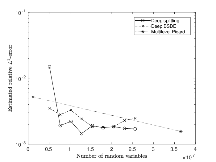
Figure 1 shows estimated relative -approximation errors as a function of the number of one-dimensional standard normal random variables used by the three methods to approximate for the solution of the sine-Gordon-type equation (3.12) for and . It can be seen that for this particular example, the three methods yield comparable results. But it has to be noted that the deep splitting algorithm and the deep BSDE method both involve different hyper-parameters, which, for good results, have to be fine-tuned depending on the form and the parameters of the PDE. Figure 1 just shows results for particular implementations of the three methods.
Generally, since the deep splitting method uses neural networks to approximate the solution of a PDE on a time grid , it can learn approximations of , , simultaneously for all . Similarly, the deep BSDE method can be implemented so that it approximates directly for all . However, for a temporal discretization with subintervals, it then needs to train neural networks at the same time, whereas the deep splitting method trains one network after the other. So even if the two approaches need a similar total number of one-dimensional standard normal random variables to achieve a given accuracy, the deep splitting method can handle larger problems since it decomposes them into smaller computational tasks which can be solved successively.
The advantage of the multilevel Picard method is that there exist theoretical bounds on the computational effort needed for a given approximation accuracy; see e.g., [29, 57, 59, 60]. However, the method needs to calculate approximations of for different space-time points separately and becomes impractical for large .
5 Conclusion
In this paper we have developed a new numerical method to approximate solutions of high-dimensional nonlinear parabolic PDEs. It splits the differential operator into a linear and a nonlinear part and uses deep learning together with the Feynman–Kac formula to iteratively solve linear approximations of the equation over small time intervals. This breaks the PDE approximation task into smaller problems that can be solved successively. As a consequence, the approach can be applied to extremely high-dimensional nonlinear PDEs. We have tested the method on Hamilton–Jacobi–Bellman equations, nonlinear Black–Scholes equations, Allen–Cahn-type equations, semilinear heat equations as well as sine-Gordon-type equations. In all cases, it has produced accurate results in high dimensions with short run times.
Acknowledgments
We are grateful to Adam Andersson for fruitful discussions. This project has been supported by the Swiss National Science Foundation Grant “Higher order numerical approximation methods for stochastic partial differential equations”, by the Deutsche Forschungsgemeinschaft under Germany’s Excellence Strategy EXC 2044-390685587, Mathematics Münster: Dynamics - Geometry - Structure and by the Nanyang Assistant Professorship Grant “Machine Learning based Algorithms in Finance and Insurance”.
References
- [1] Bally, V., and Pagès, G. A quantization algorithm for solving multi-dimensional discrete-time optimal stopping problems. Bernoulli 9, 6 (2003), 1003–1049.
- [2] Beck, C., Becker, S., Grohs, P., Jaafari, N., and Jentzen, A. Solving stochastic differential equations and Kolmogorov equations by means of deep learning. Revision requested from Journal of Scientific Computing. arXiv:1806.00421 (2018), 56 pages.
- [3] Beck, C., E, W., and Jentzen, A. Machine learning approximation algorithms for high-dimensional fully nonlinear partial differential equations and second-order backward stochastic differential equations. Journal of Nonlinear Science (2017), 1–57.
- [4] Beck, C., Hutzenthaler, M., Jentzen, A., and Kuckuck, B. An overview on deep learning-based approximation methods for partial differential equations. arXiv:2012.12348 (2020), 22 pages.
- [5] Becker, S., Braunwarth, R., Hutzenthaler, M., Jentzen, A., and von Wurstemberger, P. Numerical simulations for full history recursive multilevel Picard approximations for systems of high-dimensional partial differential equations. Accepted in Communications in Computational Physics. arXiv:2005.10206 (2020), 21 pages.
- [6] Becker, S., Cheridito, P., and Jentzen, A. Deep optimal stopping. The Journal of Machine Learning Research 20, 74 (2015), 1–25.
- [7] Bender, C., and Denk, R. A forward scheme for backward SDEs. Stochastic Processes and their Applications 117, 12 (2007), 1793–1812.
- [8] Bender, C., Schweizer, N., and Zhuo, J. A primal-dual algorithm for BSDEs. Mathematical Finance 27, 3 (2017), 866–901.
- [9] Bengio, Y. Learning deep architectures for AI. Foundations and Trends in Machine Learning 2, 1 (2009), 1–127.
- [10] Berg, J., and Nyström, K. A unified deep artificial neural network approach to partial differential equations in complex geometries. Neurocomputing 317 (2018), 28–41.
- [11] Berner, J., Grohs, P., and Jentzen, A. Analysis of the generalization error: Empirical risk minimization over deep artificial neural networks overcomes the curse of dimensionality in the numerical approximation of Black-Scholes partial differential equations. SIAM Journal on Mathematics of Data Science 2, 3 (2020), 631–657.
- [12] Bouchard, B., and Touzi, N. Discrete-time approximation and Monte-Carlo simulation of backward stochastic differential equations. Stochastic Processes and their Applications 111, 2 (2004), 175–206.
- [13] Braess, D. Finite elements, third ed. Cambridge University Press, Cambridge, 2007. Theory, fast solvers, and applications in elasticity theory, Translated from the German by Larry L. Schumaker.
- [14] Chan-Wai-Nam, Q., Mikael, J., and Warin, X. Machine learning for semi linear PDEs. Journal of Scientific Computing 79, 3 (2019), 1667–1712.
- [15] Chassagneux, J.-F. Linear multistep schemes for BSDEs. SIAM Journal on Numerical Analysis 52, 6 (2014), 2815–2836.
- [16] Chassagneux, J.-F., and Crisan, D. Runge-Kutta schemes for backward stochastic differential equations. The Annals of Applied Probability 24, 2 (2014), 679–720.
- [17] Chassagneux, J.-F., and Richou, A. Numerical stability analysis of the Euler scheme for BSDEs. SIAM Journal on Numerical Analysis 53, 2 (2015), 1172–1193.
- [18] Chassagneux, J.-F., and Richou, A. Numerical simulation of quadratic BSDEs. The Annals of Applied Probability 26, 1 (2016), 262–304.
- [19] Crisan, D., and Manolarakis, K. Probabilistic methods for semilinear partial differential equations. Applications to finance. M2AN Mathematical Modelling and Numerical Analysis 44, 5 (2010), 1107–1133.
- [20] Crisan, D., and Manolarakis, K. Solving backward stochastic differential equations using the cubature method: application to nonlinear pricing. SIAM Journal on Financial Mathematics 3, 1 (2012), 534–571.
- [21] Crisan, D., and Manolarakis, K. Second order discretization of backward SDEs and simulation with the cubature method. The Annals of Applied Probability 24, 2 (2014), 652–678.
- [22] Crisan, D., Manolarakis, K., and Touzi, N. On the Monte Carlo simulation of BSDEs: an improvement on the Malliavin weights. Stochastic Processes and their Applications 120, 7 (2010), 1133–1158.
- [23] Deck, T., and Kruse, S. Parabolic differential equations with unbounded coefficients—a generalization of the parametrix method. Acta Applicandae Mathematicae 74, 1 (2002), 71–91.
- [24] Delarue, F., and Menozzi, S. A forward-backward stochastic algorithm for quasi-linear PDEs. The Annals of Applied Probability 16, 1 (2006), 140–184.
- [25] Dörsek, P. Semigroup splitting and cubature approximations for the stochastic Navier-Stokes equations. SIAM Journal on Numerical Analysis 50, 2 (2012), 729–746.
- [26] Douglas, Jr., J., Ma, J., and Protter, P. Numerical methods for forward-backward stochastic differential equations. The Annals of Applied Probability 6, 3 (1996), 940–968.
- [27] Duffie, D., Schroder, M., and Skiadas, C. Recursive valuation of defaultable securities and the timing of resolution of uncertainty. Ann. Appl. Probab. 6, 4 (1996), 1075–1090.
- [28] E, W., Han, J., and Jentzen, A. Deep learning-based numerical methods for high-dimensional parabolic partial differential equations and backward stochastic differential equations. Communications in Mathematics and Statistics 5 (2017), 349–380.
- [29] E, W., Hutzenthaler, M., Jentzen, A., and Kruse, T. Multilevel Picard iterations for solving smooth semilinear parabolic heat equations. Revision requested from SN Partial Differential Equations and Applications. arXiv:1607.03295 (2017), 18 pages.
- [30] E, W., Hutzenthaler, M., Jentzen, A., and Kruse, T. On multilevel Picard numerical approximations for high-dimensional nonlinear parabolic partial differential equations and high-dimensional nonlinear backward stochastic differential equations. Journal of Scientific Computing (2019), 1–38.
- [31] E, W., and Yu, B. The deep Ritz method: A deep learning-based numerical algorithm for solving variational problems. Communications in Mathematics and Statistics 6, 1 (2018), 1–12.
- [32] Elbrächter, D., Grohs, P., Jentzen, A., and Schwab, C. DNN expression rate analysis of high-dimensional PDEs: Application to option pricing. Accepted in Constructive Approximation. arXiv:1809.07669 (2018), 50 pages.
- [33] Farahmand, A.-m., Nabi, S., and Nikovski, D. N. Deep reinforcement learning for partial differential equation control. 2017 American Control Conference (ACC) (2017), 3120–3127.
- [34] Fujii, M., Takahashi, A., and Takahashi, M. Asymptotic expansion as prior knowledge in deep learning method for high dimensional BSDEs. Asia-Pacific Financial Markets 26, 3 (2019), 391–408.
- [35] Glorot, X., and Bengio, Y. Understanding the difficulty of training deep feedforward neural networks. Proceedings of the thirteenth international conference on artificial intelligence and statistics (2010), 249–256.
- [36] Gobet, E., and Labart, C. Solving BSDE with adaptive control variate. SIAM Journal on Numerical Analysis 48, 1 (2010), 257–277.
- [37] Gobet, E., and Lemor, J.-P. Numerical simulation of BSDEs using empirical regression methods: theory and practice. arXiv:0806.4447 (2008), 17 pages.
- [38] Gobet, E., Lemor, J.-P., and Warin, X. A regression-based Monte Carlo method to solve backward stochastic differential equations. The Annals of Applied Probability 15, 3 (2005), 2172–2202.
- [39] Gobet, E., López-Salas, J. G., Turkedjiev, P., and Vázquez, C. Stratified regression Monte-Carlo scheme for semilinear PDEs and BSDEs with large scale parallelization on GPUs. SIAM Journal on Scientific Computing 38, 6 (2016), C652–C677.
- [40] Gobet, E., and Turkedjiev, P. Approximation of backward stochastic differential equations using Malliavin weights and least-squares regression. Bernoulli 22, 1 (2016), 530–562.
- [41] Gobet, E., and Turkedjiev, P. Linear regression MDP scheme for discrete backward stochastic differential equations under general conditions. Mathematics of Computation 85, 299 (2016), 1359–1391.
- [42] Goudenege, L., Molent, A., and Zanette, A. Machine learning for pricing American options in high-dimensional Markovian and non-Markovian models Quantitative Finance 20 4 (2020), 573–591.
- [43] Grecksch, W., and Lisei, H. Approximation of stochastic nonlinear equations of Schrödinger type by the splitting method. Stochastic Analysis and Applications 31, 2 (2013), 314–335.
- [44] Grohs, P., Hornung, F., Jentzen, A., and von Wurstemberger, P. A proof that artificial neural networks overcome the curse of dimensionality in the numerical approximation of Black-Scholes partial differential equations. Accepted in the Memoirs of the American Mathematical Society. arXiv:1809.02362 (2018), 124 pages.
- [45] Gyöngy, I., and Krylov, N. On the rate of convergence of splitting-up approximations for SPDEs. Stochastic inequalities and applications (2003), 301–321.
- [46] Gyöngy, I., and Krylov, N. On the splitting-up method and stochastic partial differential equations. The Annals of Probability 31, 2 (2003), 564–591.
- [47] Hairer, M., Hutzenthaler, M., and Jentzen, A. Loss of regularity for Kolmogorov equations. The Annals of Probability 43, 2 (2015), 468–527.
- [48] Han, J., Jentzen, A., and E, W. Solving high-dimensional partial differential equations using deep learning. Proceedings of the National Academy of Sciences 115, 34 (2018), 8505–8510.
- [49] Han, J., and Long, J. Convergence of the deep BSDE method for coupled FBSDEs. Probability, Uncertainty and Quantitative Risk 5 1 (2020), 1–33.
- [50] Henry-Labordère, P. Counterparty risk valuation: a marked branching diffusion approach. arXiv:1203.2369 (2012), 17 pages.
- [51] Henry-Labordere, P. Deep primal-dual algorithm for BSDEs: Applications of machine learning to CVA and IM. Preprint, SSRN–id3071506 (2017), 16 pages.
- [52] Henry-Labordère, P., Oudjane, N., Tan, X., Touzi, N., and Warin, X. Branching diffusion representation of semilinear PDEs and Monte Carlo approximation. Annales de l’Institut Henri Poincaré (B) Probabilités et Statistiques 55, 1 (2019), 184–210.
- [53] Henry-Labordère, P., Tan, X., and Touzi, N. A numerical algorithm for a class of BSDEs via the branching process. Stochastic Processes and their Applications 124, 2 (2014), 1112–1140.
- [54] Huijskens, T. P., Ruijter, M. J., and Oosterlee, C. W. Efficient numerical Fourier methods for coupled forward-backward SDEs. Journal of Computational and Applied Mathematics 296 (2016), 593–612.
- [55] Huré, C., Pham, H., and Warin, X. Some machine learning schemes for high-dimensional nonlinear PDEs. arXiv:1902.01599 (2019), 33 pages.
- [56] Hutzenthaler, M., Jentzen, A., Kruse, T., and Nguyen, T. A. A proof that rectified deep neural networks overcome the curse of dimensionality in the numerical approximation of semilinear heat equations. SN Partial Differential Equations and Applications 1 (2020), 1–34.
- [57] Hutzenthaler, M., Jentzen, A., Kruse, T., Nguyen, T. A., and von Wurstemberger, P. Overcoming the curse of dimensionality in the numerical approximation of semilinear parabolic partial differential equations. Accepted in Proceedings of the Royal Society of London. Series A. arXiv:1807.01212 (2018), 27 pages.
- [58] Hutzenthaler, M., Jentzen, A., and Salimova, D. Strong convergence of full-discrete nonlinearity-truncated accelerated exponential Euler-type approximations for stochastic Kuramoto-Sivashinsky equations. Communications in Mathematical Sciences 16 (2018), 1489–1529.
- [59] Hutzenthaler, M., Jentzen, A., and von Wurstemberger, P. Overcoming the curse of dimensionality in the approximative pricing of financial derivatives with default risks. Electronic Journal of Probability 25, (2020), 1–73.
- [60] Hutzenthaler, M., and Kruse, T. Multi-level Picard approximations of high-dimensional semilinear parabolic differential equations with gradient-dependent nonlinearities. SIAM Journal on Numerical Analysis 58, 2 (2020), 929–961.
- [61] Ioffe, S., and Szegedy, C. Batch Normalization: Accelerating Deep Network Training by Reducing Internal Covariate Shift. arXiv:1502.03167 (2015), 11 pages.
- [62] Jacquier, A., and Oumgari, M. Deep PPDEs for rough local stochastic volatility. arXiv:1906.02551 (2019), 21 pages.
- [63] Jentzen, A., Salimova, D., and Welti, T. A proof that deep artificial neural networks overcome the curse of dimensionality in the numerical approximation of Kolmogorov partial differential equations with constant diffusion and nonlinear drift coefficients. Accepted in Communications in Mathematical Sciences. arXiv:1809.07321 (2018), 48 pages.
- [64] Kingma, D., and Ba, J. Adam: A Method for Stochastic Optimization. arXiv:1412.6980 (2014), 15 pages.
- [65] Klenke, A. Probability theory. A comprehensive course, second ed. Universitext. Springer, London, 2014.
- [66] Kloeden, P. E., and Platen, E. Numerical solution of stochastic differential equations, vol. 23 of Applications of Mathematics (New York). Springer-Verlag, Berlin, 1992.
- [67] Krylov, N. V. Lectures on elliptic and parabolic equations in Hölder spaces, vol. 12 of Graduate Studies in Mathematics. American Mathematical Society, Providence, RI, 1996.
- [68] Krylov, N. V. On Kolmogorov’s equations for finite-dimensional diffusions. Stochastic PDE’s and Kolmogorov equations in infinite dimensions (Cetraro, 1998) 1715 (1999), 1–63.
- [69] Kutyniok, G., Petersen, P., Raslan, M., and Schneider, R. A theoretical analysis of deep neural networks and parametric PDEs. arXiv:1904.00377 (2019), 42 pages.
- [70] Labart, C., and Lelong, J. A parallel algorithm for solving BSDEs. Monte Carlo Methods and Applications 19, 1 (2013), 11–39.
- [71] Larsson, S., and Thomée, V. Partial differential equations with numerical methods, vol. 45 of Texts in Applied Mathematics. Springer-Verlag, Berlin, 2003.
- [72] LeCun, Y., Bengio, Y., and Hinton, G. Deep learning. Nature 521 (2015), 436–444.
- [73] Lemor, J.-P., Gobet, E., and Warin, X. Rate of convergence of an empirical regression method for solving generalized backward stochastic differential equations. Bernoulli 12, 5 (2006), 889–916.
- [74] Lionnet, A., dos Reis, G., and Szpruch, L. Time discretization of FBSDE with polynomial growth drivers and reaction-diffusion PDEs. The Annals of Applied Probability 25, 5 (2015), 2563–2625.
- [75] Long, Z., Lu, Y., Ma, X., and Dong, B. PDE-Net: Learning PDEs from Data. International Conference on Machine Learning (2018), 3208–3216.
- [76] Lye, K. O., Mishra, S., and Ray, D. Deep learning observables in computational fluid dynamics. Journal of Computational Physics, 109339 (2020), 1–26.
- [77] Ma, J., Protter, P., San Martín, J., and Torres, S. Numerical method for backward stochastic differential equations. The Annals of Applied Probability 12, 1 (2002), 302–316.
- [78] Ma, J., Protter, P., and Yong, J. M. Solving forward-backward stochastic differential equations explicitly—a four step scheme. Probability Theory and Related Fields 98, 3 (1994), 339–359.
- [79] Ma, J., and Yong, J. Forward-backward stochastic differential equations and their applications, vol. 1702 of Lecture Notes in Mathematics. Springer-Verlag, Berlin, 1999.
- [80] Magill, M., Qureshi, F., and de Haan, H. Neural networks trained to solve differential equations learn general representations. Advances in Neural Information Processing Systems (2018), 4075–4085.
- [81] Maruyama, G. Continuous Markov processes and stochastic equations. Rendiconti del Circolo Matematico di Palermo. Serie II 4 (1955), 48–90.
- [82] McKean, H. P. Application of Brownian motion to the equation of Kolmogorov-Petrovskii-Piskunov. Communications on Pure and Applied Mathematics 28, 3 (1975), 323–331.
- [83] Milstein, G. N. Approximate integration of stochastic differential equations. Theory of Probability & Its Applications 19, 3 (1975), 557–562.
- [84] Milstein, G. N., and Tretyakov, M. V. Numerical algorithms for forward-backward stochastic differential equations. SIAM Journal on Scientific Computing 28, 2 (2006), 561–582.
- [85] Milstein, G. N., and Tretyakov, M. V. Discretization of forward-backward stochastic differential equations and related quasi-linear parabolic equations. IMA Journal of Numerical Analysis 27, 1 (2007), 24–44.
- [86] Milstein, G. N., and Tretyakov, M. V. Solving parabolic stochastic partial differential equations via averaging over characteristics. Mathematics of Computation 78, 268 (2009), 2075–2106.
- [87] Pham, H. Feynman-Kac representation of fully nonlinear PDEs and applications. Acta Mathematica Vietnamica 40, 2 (2015), 255–269.
- [88] Raissi, M. Deep hidden physics models: Deep learning of nonlinear partial differential equations. The Journal of Machine Learning Research 19, 1 (2018), 932–955.
- [89] Ruijter, M. J., and Oosterlee, C. W. A Fourier cosine method for an efficient computation of solutions to BSDEs. SIAM Journal on Scientific Computing 37, 2 (2015), A859–A889.
- [90] Ruijter, M. J., and Oosterlee, C. W. Numerical Fourier method and second-order Taylor scheme for backward SDEs in finance. Applied Numerical Mathematics 103 (2016), 1–26.
- [91] Ruszczynski, A., and Yao, J. A dual method for backward stochastic differential equations with application to risk valuation. arXiv:1701.06234 (2017), 22 pages.
- [92] Sirignano, J., and Spiliopoulos, K. DGM: A deep learning algorithm for solving partial differential equations. Journal of Computational Physics 375 (2018), 1339–1364.
- [93] Skorokhod, A. V. Branching diffusion processes. Theory of Probability & Its Applications 9, 3 (1964), 445–449.
- [94] Stroock, D. W. Lectures on topics in stochastic differential equations, vol. 68 of Tata Institute of Fundamental Research Lectures on Mathematics and Physics. Tata Institute of Fundamental Research, Bombay; by Springer-Verlag, Berlin-New York, 1982. With notes by Satyajit Karmakar.
- [95] Thomée, V. Galerkin finite element methods for parabolic problems, vol. 25 of Springer Series in Computational Mathematics. Springer-Verlag, Berlin, 1997.
- [96] Turkedjiev, P. Two algorithms for the discrete time approximation of Markovian backward stochastic differential equations under local conditions. Electronic Journal of Probability 20 (2015), no. 50, 49.
- [97] Watanabe, S. On the branching process for Brownian particles with an absorbing boundary. Journal of Mathematics of Kyoto University 4 (1965), 385–398.
- [98] Zhang, J. A numerical scheme for BSDEs. The Annals of Applied Probability 14, 1 (2004), 459–488.