跳到论文正文
W Papers独立论文阅读器 arXiv:1907.03451 论文正文 计算阅读时间 · 0%
引用这篇论文根据当前论文元数据生成,正式投稿前建议核对。


License: arXiv.org perpetual non-exclusive license
arXiv:1907.03451v2 [cs.LG] 02 Feb 2021

General Control Functions for Causal Effect Estimation from Instrumental Variables

Aahlad Puli Affiliation: Computer Science Affiliation: New York University Email: aahlad@nyu.edu    Rajesh Ranganath Affiliation: Computer Science, Center for Data Science Affiliation: New York University Email: rajeshr@cims.nyu.edu
Abstract

Causal effect estimation relies on separating the variation in the outcome into parts due to the treatment and due to the confounders. To achieve this separation, practitioners often use external sources of randomness that only influence the treatment called instrumental variables (IVs). We study variables constructed from treatment and IV that help estimate effects, called control functions. We characterize general control functions for effect estimation in a meta-identification result. Then, we show that structural assumptions on the treatment process allow the construction of general control functions, thereby guaranteeing identification. To construct general control functions and estimate effects, we develop the general control function method (GCFN). GCFN’s first stage called variational decoupling (VDE) constructs general control functions by recovering the residual variation in the treatment given the IV. Using VDE’s control function, GCFN’s second stage estimates effects via regression. Further, we develop semi-supervised GCFN to construct general control functions using subsets of data that have both IV and confounders observed as supervision; this needs no structural treatment process assumptions. We evaluate GCFN on low and high dimensional simulated data and on recovering the causal effect of slave export on modern community trust [30].

1 Introduction

Many disciplines use observational data to estimate causal effects: economics [5], sociology [23], psychology [26], epidemiology [35], and medicine [40]. Estimating causal effects with observational data requires care due to the presence of confounders that influence both treatment and outcome. Observational causal estimators deal with confounders in one of two ways. One, they assume that all confounders are observed; an assumption called ignorability. Two, they assume a source of external randomness that has a direct influence only on the treatment. Such a source is called an instrumental variable (IV) [4, 19]. An example is college proximity as an IV to study effects of education [8].

Two common IV-based causal effect estimation methods are the two-stage least-squares method (2SLS) [21, 2, 3] and the traditional control function method (CFN) [19, 45, 43, 12]. Both methods have a common first stage: learn a distribution over the treatment conditioned on the IV. In the second stage, 2SLS regresses the outcome on simulated treatments from the first stage, while CFN’s second stage regresses the outcome on the true treatment and the error in the prediction of treatment from the first stage. The prediction error can be used to control for confounding and is thus called a control function. Though widely used, both 2SLS and CFN breakdown under certain conditions like, for example, when the outcome depends on multiplicative interactions of treatment and confounders. Further, CFN requires an additional assumption about the correlations between noise and outcome.

We study causal estimation with control functions. To estimate effects, control functions must satisfy ignorability. Our meta-identification result (1) shows that a control function satisfies ignorability if 1) the control function and IV together reconstruct the treatment, and 2) the confounder and control function together are jointly independent of the IV. We will refer to such control functions as general control functions. Effect estimation in general requires that the treatment has a chance to take any value given the control function; this is called positivity. We show positivity for general control functions holds if the IV can set treatment to any value; we call this a strong IV.

Any general control function uniquely determines the effect because it satisfies ignorability and positivity (given a strong IV). Causal identification requires effects to be uniquely determined by the observed data distribution. Thus, building general control functions using observed data guarantees causal identification. As reconstruction and marginal independence are properties of the joint distribution over observed data and control function, they can be guaranteed. Guaranteeing joint independence requires further assumptions as it involves the unobserved confounder. We show that structural assumptions on the treatment process, such as treatment being an additive function of the confounder and IV, help ensure joint independence.

To build general control functions and use them to estimate effects, we develop the general control function method (GCFN). GCFN’s first stage, called variational decoupling (VDE), constructs the general control function. VDE is a type of autoencoder where the encoder constructs the control function and the decoder reconstructs treatment from control function and IV, under the constraint that the control function and IV are independent. When VDE is perfectly solved with a decoder that reflects a structural treatment process assumption, like additivity, reconstruction and joint independence are guaranteed. Thus with a strong IV, ignorability and positivity hold which implies identification, and that effect estimation does not require structural assumptions on the outcome process like those in 2SLS and CFN. Using VDE’s general control function, GCFN’s second stage estimates the causal effect. GCFN’s second stage can be any method that relies on ignorability like matching/balancing methods [41, 13, 38] and doubly-robust methods [14].

We also consider a setting where a subset of the data has observed confounders that provide ignorability. We develop semi-supervised GCFN to estimate effects in this setting. Semi-supervised GCFN’s first stage is an augmented VDE that forces the control function to match the confounder in the subset where it is observed. This augmented VDE helps guarantee joint independence even with a decoder that does not reflect structural treatment process assumptions.

In section 4, we evaluate GCFN’s causal effect estimation on simulated data with the outcome, treatment, and IV observed. We demonstrate how GCFN produces correct effect estimates without additional assumptions on the true outcome process, whereas 2SLS, CFN, and DeepIV [18] fail to produce the correct estimate. Further, we show that GCFN performs on par with recently proposed methods DeepGMM [7] and DeepIV [18] on high-dimensional simulations from each respective paper. We also demonstrate that in data with a small subset having observed confounders, semi-supervised GCFN outperforms outcome regression on treatment and confounder within the subset. We also show recovery of the effect of slave export on current societal trust [30].

Related Work.

Classical examples of methods that use IVs include the Wald estimator [42], two-stage least-squares method (2SLS) [2, 3, 21] and control function method (CFN) [12, 19, 45, 43]. The Wald estimator assumes constant treatment effect. 2SLS’s estimation could be biased when the outcome generating process has multiplicative interactions between treatment and confounders (section A.10). Guo and Small, 2016 proved that under some assumptions, CFN improves upon 2SLS. Beyond these classical estimators, Wooldridge, 2015 discusses extensions of regression residuals for non-linear models under distributional assumptions about the noise in the treatment process. Hartford et al., 2017 developed DeepIV, a deep variant of 2SLS and Singh et al., 2019 kernelized the 2SLS algorithm. An alternative to 2SLS is the generalized method of moments (GMM) [17] which solves moment equations implied by the independence of the confounder and the IV. Bennett et al., 2019 develop a minimax GMM and use neural networks to specify moment conditions.

Given only an IV, treatment, and outcome, causal effects are not identifiable without further assumptions [6, 25]. Newey, 2013 and Chetverikov and Wilhelm, 2017 assume additive outcome processes, where the outcome process is a sum of the causal effect and zero-mean noise; such models are also called separable. Identification in separable models relies on the completeness condition [11] which requires the conditional distribution of treatment given IV to sufficiently vary with the IV. Newey, 2013, Chetverikov and Wilhelm, 2017 discuss non-parametric estimators under assumptions of monotonicity of the treatment process and shape of causal effects (for eg. UU-shaped). We focus on the setting where the outcome process cannot be represented as a sum of the causal effect and noise, often called a non-separable model [9]. Imbens and Newey, 2009 showed effect identification in non-separable models when the treatment has a continuous strictly monotonic cumulative distribution function (cdf) given the IV. Under this same condition, we can guarantee joint independence via a strictly monotonic reconstruction map which means identification holds.

1.1 Review of IVs and traditional control function theory

𝐳\boldsymbol{\mathbf{z}}ϵ\boldsymbol{\mathbf{\epsilon}}𝐭\boldsymbol{\mathbf{t}}𝐲\boldsymbol{\mathbf{y}}
Figure 1: Causal graph with hidden confounder 𝐳\boldsymbol{\mathbf{z}}, outcome 𝐲\boldsymbol{\mathbf{y}}, instrument ϵ\boldsymbol{\mathbf{\epsilon}}, treatment 𝐭\boldsymbol{\mathbf{t}}.

To define the causal effect we use causal graphs [31]. In causal graphs, each variable is represented by a node, and each causal relationship is a directed arrow from the cause to the effect. Causal graphs get transformed by interventions with the do-operator. The shared relationships between the graphs before and after the do-operation make estimation possible. The causal effect of giving a treatment 𝐭=a\boldsymbol{\mathbf{t}}=a on an outcome 𝐲\boldsymbol{\mathbf{y}} is 𝔼​[𝐲|do​(𝐭=a)]\mathbb{E}[\boldsymbol{\mathbf{y}}~|~\text{do}(\boldsymbol{\mathbf{t}}=a)]. The causal graph in Figure 1 describes a broad class of IV problems. The difficulty of causal estimation in this graph stems from the unobserved confounder 𝐳\boldsymbol{\mathbf{z}}. The IV ϵ\boldsymbol{\mathbf{\epsilon}} helps control for 𝐳\boldsymbol{\mathbf{z}}. Two popular IV-based methods are the two-stage least-squares method (2SLS) and control function method (CFN).

We follow the CFN setup from Guo and Small, 2016, where the true outcome and treatment processes have additive zero-mean noise called 𝜼𝐲\boldsymbol{\mathbf{\eta}}_{\boldsymbol{\mathbf{y}}} and 𝜼𝐭\boldsymbol{\mathbf{\eta}}_{\boldsymbol{\mathbf{t}}} that may be correlated due to 𝐳\boldsymbol{\mathbf{z}}:

𝐲=f⁡(𝐭)+𝜼𝐲,𝐭=g⁡(ϵ)+𝜼𝐭.\displaystyle\boldsymbol{\mathbf{y}}=f(\boldsymbol{\mathbf{t}})+\boldsymbol{\mathbf{\eta}}_{\boldsymbol{\mathbf{y}}},\quad\boldsymbol{\mathbf{t}}=g(\boldsymbol{\mathbf{\epsilon}})+\boldsymbol{\mathbf{\eta}}_{\boldsymbol{\mathbf{t}}}. (1)

To estimate the causal effect, the CFN method constructs a control function with the regression residual 𝐭−g^​(ϵ)\boldsymbol{\mathbf{t}}-\hat{g}(\boldsymbol{\mathbf{\epsilon}}). Then, CFN regresses the outcome 𝐲\boldsymbol{\mathbf{y}} on the regression residual and the treatment 𝐭\boldsymbol{\mathbf{t}}. The causal effect is the estimate of the function f⁡(𝐭)f(\boldsymbol{\mathbf{t}}). For this estimate to be valid, the CFN method assumes that 𝜼𝐭,𝜼𝐲\boldsymbol{\mathbf{\eta}}_{\boldsymbol{\mathbf{t}}},\boldsymbol{\mathbf{\eta}}_{\boldsymbol{\mathbf{y}}} satisfy the following property for some constant ρ\rho, (assumption A4 in [16]):

𝔼⁡[𝜼𝐲|𝜼𝐭=η]=ρ​η\displaystyle\mathbb{E}[\boldsymbol{\mathbf{\eta}}_{\boldsymbol{\mathbf{y}}}~|~\boldsymbol{\mathbf{\eta}}_{\boldsymbol{\mathbf{t}}}=\eta]=\rho\eta (2)

This property restricts the applicability of the CFN method by limiting how confounders influence the outcome and the treatment. Consider the following additive noise example: ϵ,𝐳∼𝒩⁡(0,1),𝐭=𝐳+ϵ,𝐲∼𝒩⁡(𝐭2+𝐳2,1)\,\,\boldsymbol{\mathbf{\epsilon}},\boldsymbol{\mathbf{z}}\sim\mathcal{N}(0,1),\,\,\boldsymbol{\mathbf{t}}=\boldsymbol{\mathbf{z}}+\boldsymbol{\mathbf{\epsilon}},\,\,\boldsymbol{\mathbf{y}}\sim\mathcal{N}(\boldsymbol{\mathbf{t}}^{2}+\boldsymbol{\mathbf{z}}^{2},1), where 𝒩\mathcal{N} is the standard normal. Here 𝜼y=𝐳2\boldsymbol{\mathbf{\eta}}_{y}=\boldsymbol{\mathbf{z}}^{2} and 𝜼𝐭=𝐳\boldsymbol{\mathbf{\eta}}_{\boldsymbol{\mathbf{t}}}=\boldsymbol{\mathbf{z}} meaning that 𝔼⁡[𝜼𝐲|𝜼𝐭=η]=η2\mathbb{E}[\boldsymbol{\mathbf{\eta}}_{\boldsymbol{\mathbf{y}}}~|~\boldsymbol{\mathbf{\eta}}_{\boldsymbol{\mathbf{t}}}=\eta]=\eta^{2}, violating the assumption in eq. 2. Note that 𝔼⁡[𝐳𝐭2]=𝔼⁡[𝐳𝐳2]=0\mathbb{E}[\boldsymbol{\mathbf{z}}\boldsymbol{\mathbf{t}}^{2}]=\mathbb{E}[\boldsymbol{\mathbf{z}}\boldsymbol{\mathbf{z}}^{2}]=0, however 𝔼⁡[𝐭2​𝐳2]>0\mathbb{E}[\boldsymbol{\mathbf{t}}^{2}\boldsymbol{\mathbf{z}}^{2}]>0. This means regressing 𝐲\boldsymbol{\mathbf{y}} on 𝐭2\boldsymbol{\mathbf{t}}^{2} and 𝐳\boldsymbol{\mathbf{z}}, i.e., with the correct model for f⁡(𝐭)f(\boldsymbol{\mathbf{t}}), would result in an inflated coefficient of 𝐭2\boldsymbol{\mathbf{t}}^{2}, which is an incorrect causal estimate. Equation 2 is required because some specified function of 𝐭\boldsymbol{\mathbf{t}} could be correlated with an unspecified function of 𝐳\boldsymbol{\mathbf{z}}, resulting in a biased causal estimate. See section A.10 for an example where 2SLS produces biased effect estimates. The assumption in eq. 1 restricts the confounder’s influence to be additive on both the treatment and outcome. Further, CFN assumes that the average additive influence the confounder has on the outcome to be a scaled version of the confounder’s influence on the treatment (eq. 2). Such assumptions may not hold in real data. For example, the effect of a medical treatment on patient lifespan is confounded by the patient’s current health. This confounder influences the treatment through a human decision process, while it influences the outcome through a physiological process making it unlikely to meet CFN’s assumptions.

2 Causal Identification with General Control Functions

With a control function that satisfies ignorability and positivity, causal estimation reduces to regression of the outcome on the treatment and the control function. We characterize such control functions:

Theorem 1.

(Meta-identification result for control functions)
Let F⁡(𝐭,ϵ,𝐲)F(\boldsymbol{\mathbf{t}},\boldsymbol{\mathbf{\epsilon}},\boldsymbol{\mathbf{y}}) be the true data distribution. Let control function 𝐳^\hat{\boldsymbol{\mathbf{z}}} be sampled conditionally on 𝐭,ϵ\boldsymbol{\mathbf{t}},\boldsymbol{\mathbf{\epsilon}}. Let q⁡(𝐳^,𝐭,ϵ)=q⁡(𝐳^|𝐭,ϵ)​F​(𝐭,ϵ)q(\hat{\boldsymbol{\mathbf{z}}},\boldsymbol{\mathbf{t}},\boldsymbol{\mathbf{\epsilon}})=q(\hat{\boldsymbol{\mathbf{z}}}~|~\boldsymbol{\mathbf{t}},\boldsymbol{\mathbf{\epsilon}})F(\boldsymbol{\mathbf{t}},\boldsymbol{\mathbf{\epsilon}}) be the joint distribution over 𝐳^,𝐭,ϵ\hat{\boldsymbol{\mathbf{z}}},\boldsymbol{\mathbf{t}},\boldsymbol{\mathbf{\epsilon}}. Further, let gg be a deterministic function and 𝛅\boldsymbol{\mathbf{\delta}} be independent noise such that 𝐭=g⁡(𝐳,ϵ,𝛅)\boldsymbol{\mathbf{t}}=g(\boldsymbol{\mathbf{z}},\boldsymbol{\mathbf{\epsilon}},\boldsymbol{\mathbf{\delta}}) and let the implied true joint be F′​(𝐭,𝐳,𝛅)F^{\prime}(\boldsymbol{\mathbf{t}},\boldsymbol{\mathbf{z}},\boldsymbol{\mathbf{\delta}}). Assume the following:

  1. 1.

    (A1) 𝐳^\hat{\boldsymbol{\mathbf{z}}} satisfies the reconstruction property: ∃d,𝐳^,𝐭,ϵ∼q⁡(𝐳^,𝐭,ϵ)⟹𝐭=d⁡(𝐳^,ϵ)\exists d,\,\hat{\boldsymbol{\mathbf{z}}},\boldsymbol{\mathbf{t}},\boldsymbol{\mathbf{\epsilon}}\sim q(\hat{\boldsymbol{\mathbf{z}}},\boldsymbol{\mathbf{t}},\boldsymbol{\mathbf{\epsilon}})\implies\boldsymbol{\mathbf{t}}=d(\hat{\boldsymbol{\mathbf{z}}},\boldsymbol{\mathbf{\epsilon}}).

  2. 2.

    (A2) The IV is jointly independent of control function, true confounder, and noise 𝜹\boldsymbol{\mathbf{\delta}}: ϵ⊧(𝐳,𝐳^,𝜹)\boldsymbol{\mathbf{\epsilon}}\rotatebox[origin]{90.0}{$\models$}(\boldsymbol{\mathbf{z}},\hat{\boldsymbol{\mathbf{z}}},\boldsymbol{\mathbf{\delta}}).

  3. 3.

    (A3) Strong IV. For any compact B⊆supp​(𝐭)B\subseteq\textrm{supp}(\boldsymbol{\mathbf{t}}), ∃cB​s.t. a.e. ​t∈B\exists c_{B}\,\textrm{s.t.\ a.e.\ }t\in B, F′​(𝐭=t|𝐳,𝜹)≥cB>0.F^{\prime}(\boldsymbol{\mathbf{t}}=t~|~\boldsymbol{\mathbf{z}},\boldsymbol{\mathbf{\delta}})\geq c_{B}>0.

Then, the control function 𝐳^\hat{\boldsymbol{\mathbf{z}}} satisfies ignorability and positivity:

q⁡(𝐲|𝐭=t,𝐳^)=q⁡(𝐲|do​(𝐭=t),𝐳^)a.e. in supp​(𝐭)q⁡(𝐳^)>0⟹q⁡(𝐭=t|𝐳^)>0.\displaystyle q(\boldsymbol{\mathbf{y}}~|~\boldsymbol{\mathbf{t}}=t,\hat{\boldsymbol{\mathbf{z}}})=q(\boldsymbol{\mathbf{y}}~|~\emph{\text{do}}(\boldsymbol{\mathbf{t}}=t),\hat{\boldsymbol{\mathbf{z}}})\quad\quad\emph{\text{a.e. in }}\textrm{supp}(\boldsymbol{\mathbf{t}})\quad q(\hat{\boldsymbol{\mathbf{z}}})>0\implies q(\boldsymbol{\mathbf{t}}=t~|~\hat{\boldsymbol{\mathbf{z}}})>0.

Therefore, the true causal effect is uniquely determined by q⁡(𝐳^,𝐭,𝐲)q(\hat{\boldsymbol{\mathbf{z}}},\boldsymbol{\mathbf{t}},\boldsymbol{\mathbf{y}}) for almost every t∈supp​(𝐭)t\in\textrm{supp}(\boldsymbol{\mathbf{t}}):

𝔼𝐳^[𝐲|𝐭=t,𝐳^]\displaystyle\mathbb{E}_{\hat{\boldsymbol{\mathbf{z}}}}[\boldsymbol{\mathbf{y}}~|~\boldsymbol{\mathbf{t}}=t,\hat{\boldsymbol{\mathbf{z}}}] =𝔼𝐳^[𝐲|do(𝐭=t),𝐳^]=𝔼[𝐲|do(𝐭=t)].\displaystyle=\mathbb{E}_{\hat{\boldsymbol{\mathbf{z}}}}[\boldsymbol{\mathbf{y}}~|~\emph{\text{do}}(\boldsymbol{\mathbf{t}}=t),\hat{\boldsymbol{\mathbf{z}}}]=\mathbb{E}[\boldsymbol{\mathbf{y}}~|~\emph{\text{do}}(\boldsymbol{\mathbf{t}}=t)].

1 characterizes functions of treatment and IV that satisfy reconstruction (A1) and joint independence (A2) which we call general control functions. Positivity of 𝐭\boldsymbol{\mathbf{t}} w.r.t. the general control function holds under an assumption about the treatment process that the IV is strong (A3). Ignorability and positivity w.r.t. 𝐳^\hat{\boldsymbol{\mathbf{z}}} imply that the true causal effect is uniquely determined as a function of the observed data distribution q⁡(𝐳^,𝐭,𝐲)q(\hat{\boldsymbol{\mathbf{z}}},\boldsymbol{\mathbf{t}},\boldsymbol{\mathbf{y}}) 11 1 We also require that 𝔼𝐳^𝔼[𝐲|do(𝐭),𝐳^]\mathbb{E}_{\hat{\boldsymbol{\mathbf{z}}}}\mathbb{E}[\boldsymbol{\mathbf{y}}~|~\text{do}(\boldsymbol{\mathbf{t}}),\hat{\boldsymbol{\mathbf{z}}}] exists. This is guaranteed if the causal effect 𝔼[𝐲|do(𝐭)]=𝔼𝐳𝔼[𝐲|𝐭,𝐳]\mathbb{E}[\boldsymbol{\mathbf{y}}~|~\text{do}(\boldsymbol{\mathbf{t}})]=\mathbb{E}_{\boldsymbol{\mathbf{z}}}\mathbb{E}[\boldsymbol{\mathbf{y}}~|~\boldsymbol{\mathbf{t}},\boldsymbol{\mathbf{z}}] exists as ignorability holds w.r.t. 𝐳^\hat{\boldsymbol{\mathbf{z}}}: 𝔼𝐳^𝔼[𝐲|do(𝐭),𝐳^]=𝔼𝐳^𝔼q⁡(𝐳|𝐳^)𝔼[𝐲|𝐭,𝐳]=𝔼𝐳𝔼[𝐲|𝐭,𝐳]\mathbb{E}_{\hat{\boldsymbol{\mathbf{z}}}}\mathbb{E}[\boldsymbol{\mathbf{y}}~|~\text{do}(\boldsymbol{\mathbf{t}}),\hat{\boldsymbol{\mathbf{z}}}]=\mathbb{E}_{\hat{\boldsymbol{\mathbf{z}}}}\mathbb{E}_{q(\boldsymbol{\mathbf{z}}~|~\hat{\boldsymbol{\mathbf{z}}})}\mathbb{E}[\boldsymbol{\mathbf{y}}~|~\boldsymbol{\mathbf{t}},\boldsymbol{\mathbf{z}}]=\mathbb{E}_{\boldsymbol{\mathbf{z}}}\mathbb{E}[\boldsymbol{\mathbf{y}}~|~\boldsymbol{\mathbf{t}},\boldsymbol{\mathbf{z}}]. . If A1 and A2 are satisfied by the observed data distribution q⁡(𝐳^,𝐭,𝐲,ϵ)q(\hat{\boldsymbol{\mathbf{z}}},\boldsymbol{\mathbf{t}},\boldsymbol{\mathbf{y}},\boldsymbol{\mathbf{\epsilon}}), the true effect is uniquely determined by the observed data distribution and thus causal identification holds. However, joint independence (A2) relies on the unobserved true confounder 𝐳\boldsymbol{\mathbf{z}}. So, 1 is a meta-identification result because it does not specify how to guarantee joint independence using q⁡(𝐳^,𝐭,ϵ)q(\hat{\boldsymbol{\mathbf{z}}},\boldsymbol{\mathbf{t}},\boldsymbol{\mathbf{\epsilon}}). In section 2.1, we discuss structural assumptions on the treatment process that instantiate this meta-result and guarantee identification.

1 holds for both discrete and continuous 𝐭\boldsymbol{\mathbf{t}} given that the causal effect exists for all t∈supp​(𝐭)t\in\textrm{supp}(\boldsymbol{\mathbf{t}}).22 2 Effects for certain treatments can be identified even without the strong IV assumption (A3): for any compact subset B⊆supp​(𝐭)B\subseteq\textrm{supp}(\boldsymbol{\mathbf{t}}) such that ∀t∈B,F′​(𝐭=t|𝐳,𝜹)≥cB>0\forall t\in B,\,\,F^{\prime}(\boldsymbol{\mathbf{t}}=t~|~\boldsymbol{\mathbf{z}},\boldsymbol{\mathbf{\delta}})\geq c_{B}>0, effects can be estimated for all t∈Bt\in B. While we focus on the causal effect 𝔼​[𝐲|do​(𝐭)]\mathbb{E}[\boldsymbol{\mathbf{y}}~|~\text{do}(\boldsymbol{\mathbf{t}})], 1 guarantees any property of 𝐲|do​(𝐭)\boldsymbol{\mathbf{y}}~|~\text{do}(\boldsymbol{\mathbf{t}}) can be estimated; for e.g. quantile treatment effects. For ease of exposition, we restrict ourselves to treatments of the form 𝐭=g⁡(ϵ,𝐳)\boldsymbol{\mathbf{t}}=g(\boldsymbol{\mathbf{\epsilon}},\boldsymbol{\mathbf{z}}), without noise 𝜹\boldsymbol{\mathbf{\delta}}. Then, 1 requires only ϵ⊧(𝐳,𝐳^)\boldsymbol{\mathbf{\epsilon}}\rotatebox[origin]{90.0}{$\models$}(\boldsymbol{\mathbf{z}},\hat{\boldsymbol{\mathbf{z}}}). In section A.6, we show ϵ⊧(𝐳^,𝐳,𝜹)\boldsymbol{\mathbf{\epsilon}}\rotatebox[origin]{90.0}{$\models$}(\hat{\boldsymbol{\mathbf{z}}},\boldsymbol{\mathbf{z}},\boldsymbol{\mathbf{\delta}}) is guaranteed for more general treatment processes of the form 𝐭=g⁡(ϵ,h⁡(𝐳,𝜹))\boldsymbol{\mathbf{t}}=g(\boldsymbol{\mathbf{\epsilon}},h(\boldsymbol{\mathbf{z}},\boldsymbol{\mathbf{\delta}})). Guaranteeing joint independence requires further conditions and is the central challenge in developing two-stage IV-based estimators.

Why joint independence?

A potential outcome 𝐲𝐭\boldsymbol{\mathbf{y}}_{\boldsymbol{\mathbf{t}}} is the outcome that would be observed if a unit is given treatment 𝐭\boldsymbol{\mathbf{t}}. The potential outcome 𝐲𝐭\boldsymbol{\mathbf{y}}_{\boldsymbol{\mathbf{t}}} follows the distribution of 𝐲\boldsymbol{\mathbf{y}} under the d​odo operator and only depends on the true confounder 𝐳\boldsymbol{\mathbf{z}}. For ignorability with respect to 𝐳^\hat{\boldsymbol{\mathbf{z}}}, we need 𝐲𝐭\boldsymbol{\mathbf{y}}_{\boldsymbol{\mathbf{t}}} to be independent of 𝐭\boldsymbol{\mathbf{t}}, given 𝐳^\hat{\boldsymbol{\mathbf{z}}}. By reconstruction, given 𝐳^\hat{\boldsymbol{\mathbf{z}}}, 𝐭\boldsymbol{\mathbf{t}} is purely a function of ϵ\boldsymbol{\mathbf{\epsilon}}. This means ignorability with respect to the control function 𝐳^\hat{\boldsymbol{\mathbf{z}}} requires that the true confounder and IV be independent given the control function. Therefore, ignorability requires 𝐳⊧ϵ|𝐳^\boldsymbol{\mathbf{z}}\rotatebox[origin]{90.0}{$\models$}\boldsymbol{\mathbf{\epsilon}}~|~\hat{\boldsymbol{\mathbf{z}}}. Further, conditional independence 𝐳^⊧ϵ|𝐳\hat{\boldsymbol{\mathbf{z}}}\rotatebox[origin]{90.0}{$\models$}\boldsymbol{\mathbf{\epsilon}}~|~\boldsymbol{\mathbf{z}} implies positivity of 𝐭\boldsymbol{\mathbf{t}} w.r.t 𝐳^\hat{\boldsymbol{\mathbf{z}}} if ϵ\boldsymbol{\mathbf{\epsilon}} is strong. Joint independence ϵ⊧(𝐳,𝐳^)\boldsymbol{\mathbf{\epsilon}}\rotatebox[origin]{90.0}{$\models$}(\boldsymbol{\mathbf{z}},\hat{\boldsymbol{\mathbf{z}}}) implies both the conditional independencies above.

The causal graph fig. 1 with 𝐲\boldsymbol{\mathbf{y}} marginalized out can be represented with two sources of randomness one from the unobserved confounder 𝐳\boldsymbol{\mathbf{z}} and one from the IV ϵ\boldsymbol{\mathbf{\epsilon}}; the extra randomness in 𝐭\boldsymbol{\mathbf{t}} denoted as 𝜹\boldsymbol{\mathbf{\delta}} can be absorbed into 𝐳\boldsymbol{\mathbf{z}}. In this setup, the treatment and control function are deterministic functions of the unobserved confounder and IV. With only two sources of randomness, joint independence means the control function 𝐳^\hat{\boldsymbol{\mathbf{z}}} needs to only be a function of the true unobserved confounder 𝐳\boldsymbol{\mathbf{z}}. When 𝐳^\hat{\boldsymbol{\mathbf{z}}} is a stochastic function of the treatment and IV, joint independence holds if 𝐳^\hat{\boldsymbol{\mathbf{z}}} determines 𝐳\boldsymbol{\mathbf{z}} while 𝐳^⊧ϵ\hat{\boldsymbol{\mathbf{z}}}\rotatebox[origin]{90.0}{$\models$}\boldsymbol{\mathbf{\epsilon}}.

As 𝐳^\hat{\boldsymbol{\mathbf{z}}} and ϵ\boldsymbol{\mathbf{\epsilon}} are observed, we can guarantee 𝐳^⊧ϵ\hat{\boldsymbol{\mathbf{z}}}\rotatebox[origin]{90.0}{$\models$}\boldsymbol{\mathbf{\epsilon}}. The marginal independence 𝐳⊧ϵ\boldsymbol{\mathbf{z}}\rotatebox[origin]{90.0}{$\models$}\boldsymbol{\mathbf{\epsilon}} holds by definition of an IV. However, even both marginal independencies 𝐳^⊧ϵ\hat{\boldsymbol{\mathbf{z}}}\rotatebox[origin]{90.0}{$\models$}\boldsymbol{\mathbf{\epsilon}} and 𝐳⊧ϵ\boldsymbol{\mathbf{z}}\rotatebox[origin]{90.0}{$\models$}\boldsymbol{\mathbf{\epsilon}} together do not imply joint independence ϵ⊧(𝐳^,𝐳)\boldsymbol{\mathbf{\epsilon}}\rotatebox[origin]{90.0}{$\models$}(\hat{\boldsymbol{\mathbf{z}}},\boldsymbol{\mathbf{z}}). This means a control function 𝐳^\hat{\boldsymbol{\mathbf{z}}} that satisfies the reconstruction property and marginal independence 𝐳^⊧ϵ\hat{\boldsymbol{\mathbf{z}}}\rotatebox[origin]{90.0}{$\models$}\boldsymbol{\mathbf{\epsilon}} may fail to yield ignorability. In section A.4, we build an example of a deterministic almost everywhere invertible function of two independent variables 𝐜=f⁡(𝐚,𝐛)\boldsymbol{\mathbf{c}}=f(\boldsymbol{\mathbf{a}},\boldsymbol{\mathbf{b}}) such that 𝐜⊧𝐚\boldsymbol{\mathbf{c}}\rotatebox[origin]{90.0}{$\models$}\boldsymbol{\mathbf{a}} and 𝐜⊧𝐛\boldsymbol{\mathbf{c}}\rotatebox[origin]{90.0}{$\models$}\boldsymbol{\mathbf{b}} and yet, joint independence (𝐜,𝐛)⊧̸𝐚(\boldsymbol{\mathbf{c}},\boldsymbol{\mathbf{b}})\rotatebox[origin]{90.0}{$\not\models$}\boldsymbol{\mathbf{a}} is violated. As 𝐳\boldsymbol{\mathbf{z}} is unobserved, achieving joint independence requires further assumptions. Next, we discuss how structural assumptions on the true treatment process can help guarantee joint independence.

2.1 Guaranteeing joint independence for identification

We show structural treatment process assumptions help guarantee joint independence by relating it to q⁡(𝐳^,𝐭,ϵ)q(\hat{\boldsymbol{\mathbf{z}}},\boldsymbol{\mathbf{t}},\boldsymbol{\mathbf{\epsilon}}) and thus giving identification. Joint independence can be guaranteed (via marginal independence) if the reconstruction map d⁡(𝐳^,ϵ)d(\hat{\boldsymbol{\mathbf{z}}},\boldsymbol{\mathbf{\epsilon}}) (A1, 1) reflects the functional structure of the treatment process. As an example, consider an additive treatment process 𝐭=𝐳+g⁡(ϵ)\boldsymbol{\mathbf{t}}=\boldsymbol{\mathbf{z}}+g(\boldsymbol{\mathbf{\epsilon}}). If the reconstruction map is d⁡(𝐳^,ϵ)=h′​(𝐳^)+g′​(ϵ)d(\hat{\boldsymbol{\mathbf{z}}},\boldsymbol{\mathbf{\epsilon}})=h^{\prime}(\hat{\boldsymbol{\mathbf{z}}})+g^{\prime}(\boldsymbol{\mathbf{\epsilon}}) and ϵ⊧𝐳^\boldsymbol{\mathbf{\epsilon}}\rotatebox[origin]{90.0}{$\models$}\hat{\boldsymbol{\mathbf{z}}}, joint independence holds. To see this, note

h′​(𝐳^)−𝔼𝐳^​[h′​(𝐳^)]=𝐭−𝔼⁡[𝐭|ϵ]=𝐳−𝔼𝐳​[𝐳]⟹∃ constant ​c,h′​(𝐳^)=𝐳+c,\displaystyle h^{\prime}(\hat{\boldsymbol{\mathbf{z}}})-\mathbb{E}_{\hat{\boldsymbol{\mathbf{z}}}}[h^{\prime}(\hat{\boldsymbol{\mathbf{z}}})]=\boldsymbol{\mathbf{t}}-\mathbb{E}[\boldsymbol{\mathbf{t}}~|~\boldsymbol{\mathbf{\epsilon}}]=\boldsymbol{\mathbf{z}}-\mathbb{E}_{\boldsymbol{\mathbf{z}}}[\boldsymbol{\mathbf{z}}]\implies\exists\text{ constant }c,\,h^{\prime}(\hat{\boldsymbol{\mathbf{z}}})=\boldsymbol{\mathbf{z}}+c, (3)

meaning h′​(𝐳^)h^{\prime}(\hat{\boldsymbol{\mathbf{z}}}) determines 𝐳\boldsymbol{\mathbf{z}}. By 𝐳^⊧ϵ\hat{\boldsymbol{\mathbf{z}}}\rotatebox[origin]{90.0}{$\models$}\boldsymbol{\mathbf{\epsilon}}, it holds that q⁡(𝐳^,𝐳|ϵ)=q⁡(𝐳^,h′​(𝐳^)−c|ϵ)=q⁡(𝐳^,𝐳).q(\hat{\boldsymbol{\mathbf{z}}},\boldsymbol{\mathbf{z}}~|~\boldsymbol{\mathbf{\epsilon}})=q(\hat{\boldsymbol{\mathbf{z}}},h^{\prime}(\hat{\boldsymbol{\mathbf{z}}})-c~|~\boldsymbol{\mathbf{\epsilon}})=q(\hat{\boldsymbol{\mathbf{z}}},\boldsymbol{\mathbf{z}}). Thus, leveraging the functional structure of the treatment process helps guarantee joint independence by relating it to q⁡(𝐳^,𝐭,ϵ)q(\hat{\boldsymbol{\mathbf{z}}},\boldsymbol{\mathbf{t}},\boldsymbol{\mathbf{\epsilon}}), via 𝐳^⊧ϵ\hat{\boldsymbol{\mathbf{z}}}\rotatebox[origin]{90.0}{$\models$}\boldsymbol{\mathbf{\epsilon}}. Assuming treatment gets generated from other known invertible functions, such as multiplication 𝐭=h⁡(𝐳)∗g⁡(ϵ)\boldsymbol{\mathbf{t}}=h(\boldsymbol{\mathbf{z}})*g(\boldsymbol{\mathbf{\epsilon}}), also leads to joint independence. Imbens and Newey, 2009 proved effect identification when the treatment is a continuous strictly monotonic function of the confounder; these conditions helps guarantee joint independence (see section A.7). For more general treatments of the form 𝐭=g⁡(ϵ,h⁡(𝐳,𝜹))\boldsymbol{\mathbf{t}}=g(\boldsymbol{\mathbf{\epsilon}},h(\boldsymbol{\mathbf{z}},\boldsymbol{\mathbf{\delta}})) the structural assumptions from above can only guarantee (h⁡(𝐳,𝜹),𝐳^)⊧ϵ(h(\boldsymbol{\mathbf{z}},\boldsymbol{\mathbf{\delta}}),\hat{\boldsymbol{\mathbf{z}}})\rotatebox[origin]{90.0}{$\models$}\boldsymbol{\mathbf{\epsilon}}; see section A.5 for general additive treatments: 𝐭=h⁡(𝐳,𝜹)+g⁡(ϵ)\boldsymbol{\mathbf{t}}=h(\boldsymbol{\mathbf{z}},\boldsymbol{\mathbf{\delta}})+g(\boldsymbol{\mathbf{\epsilon}}). However, we show in section A.6 that for such general treatment processes (h⁡(𝐳,𝜹),𝐳^)⊧ϵ⟹(𝐳,𝐳^,𝜹)⊧ϵ(h(\boldsymbol{\mathbf{z}},\boldsymbol{\mathbf{\delta}}),\hat{\boldsymbol{\mathbf{z}}})\rotatebox[origin]{90.0}{$\models$}\boldsymbol{\mathbf{\epsilon}}\implies(\boldsymbol{\mathbf{z}},\hat{\boldsymbol{\mathbf{z}}},\boldsymbol{\mathbf{\delta}})\rotatebox[origin]{90.0}{$\models$}\boldsymbol{\mathbf{\epsilon}} which, together with reconstruction, implies ignorability(1). In summary, under certain structural assumptions, general control functions exist (𝐳^=𝐳\hat{\boldsymbol{\mathbf{z}}}=\boldsymbol{\mathbf{z}} for example) and can be built using only properties of the observed data distribution q⁡(𝐳^,𝐭,ϵ)q(\hat{\boldsymbol{\mathbf{z}}},\boldsymbol{\mathbf{t}},\boldsymbol{\mathbf{\epsilon}}). This guarantees identification. In section 3, we develop practical algorithms to build general control functions.

2.2 Comparison of identification with general control functions to existing work

Traditional CFN theory [16] relies on the assumption that the treatment process is additive; recall 𝐭=g⁡(ϵ)+𝜼t\boldsymbol{\mathbf{t}}=g(\boldsymbol{\mathbf{\epsilon}})+\boldsymbol{\mathbf{\eta}}_{t} from section 1.1 and 𝜼t\boldsymbol{\mathbf{\eta}}_{t} is correlated with outcome noise due to 𝐳\boldsymbol{\mathbf{z}}. Beyond this additivity assumption, traditional CFN theory further assumes 1) the outcome process is additive, like in eq. 1, 2) the noise 𝜼y\boldsymbol{\mathbf{\eta}}_{y} in the outcome process is independent of the IV, 3) linear noise relationship between 𝜼t,𝜼y\boldsymbol{\mathbf{\eta}}_{t},\boldsymbol{\mathbf{\eta}}_{y}, like in eq. 2, and 4) (relevance) the treatment effect function and IV are correlated [16]. When the treatment process is additive, joint independence can be guaranteed as a property of the distribution q⁡(𝐳^,𝐭,ϵ)q(\hat{\boldsymbol{\mathbf{z}}},\boldsymbol{\mathbf{t}},\boldsymbol{\mathbf{\epsilon}}), via 𝐳^⊧ϵ\hat{\boldsymbol{\mathbf{z}}}\rotatebox[origin]{90.0}{$\models$}\boldsymbol{\mathbf{\epsilon}}; see section 2.1. Then, identification with general control functions requires a strong IV. While it allows structural outcome process assumptions (like 3) can be relaxed, a strong IV needs more than the two IV properties, independence with confounder and relevance. However, domain expertise helps reason about strong IVs; for example, can college proximity influence a student’s decision to go to college regardless of skill? If yes, college proximity is a strong IV. We compare against other identification conditions (like 2SLS and [20]) in section A.8.

3 The General Control Function Method (GCFN)

GCFN constructs a general control function and estimates effects with it. GCFN has two stages. The first stage constructs a general control function as the code of an autoencoder. The second stage builds a model from the control function and the treatment to the outcome and estimates effects.

Variational Decoupling

We construct the control function 𝐳^\hat{\boldsymbol{\mathbf{z}}} as a stochastic function of the treatment 𝐭\boldsymbol{\mathbf{t}} and the IV ϵ\boldsymbol{\mathbf{\epsilon}}; with parameter θ\theta, the estimator is qθ​(𝐳^|𝐭,ϵ)q_{\theta}(\hat{\boldsymbol{\mathbf{z}}}~|~\boldsymbol{\mathbf{t}},\boldsymbol{\mathbf{\epsilon}}). First, to guarantee the reconstruction property (A1 in 1), the control function and the IV must determine treatment, implying that with parameter ϕ\phi, pϕ​(𝐭|𝐳^=z^,ϵ)p_{\phi}(\boldsymbol{\mathbf{t}}~|~\hat{\boldsymbol{\mathbf{z}}}=\hat{z},\boldsymbol{\mathbf{\epsilon}}) should be maximized for z^∼q⁡(𝐳^|𝐭,ϵ)\hat{z}\sim q(\hat{\boldsymbol{\mathbf{z}}}~|~\boldsymbol{\mathbf{t}},\boldsymbol{\mathbf{\epsilon}}). Together, these form the parts of an autoencoder where a control function is sampled conditioned on the treatment and IV, while the treatment is reconstructed from the same control function and IV. Second, to guarantee marginal independence, we force the control function to be independent of the IV: 𝐳^⊧ϵ\hat{\boldsymbol{\mathbf{z}}}\rotatebox[origin]{90.0}{$\models$}\boldsymbol{\mathbf{\epsilon}}. Let the true data distribution be F⁡(𝐭,ϵ)F(\boldsymbol{\mathbf{t}},\boldsymbol{\mathbf{\epsilon}}) and 𝐈\mathbf{I} denote mutual information. Putting the two parts together, we define a constrained optimization to construct 𝐳^\hat{\boldsymbol{\mathbf{z}}}, called variational decoupling (VDE):

(VDE)maxθ,ϕ𝔼F⁡(𝐭,ϵ)​𝔼qθ​(𝐳^|𝐭,ϵ)​log⁡pϕ​(𝐭|𝐳^,ϵ)s.t𝐈θ​(𝐳^,ϵ)=0.\displaystyle\begin{split}\text{(\lx@glossaries@gls@link{acronym}{vde}{{{}}{\color[rgb]{0,0,0}VDE}})}\quad\max_{\theta,\phi}&\,\mathbb{E}_{F(\boldsymbol{\mathbf{t}},\boldsymbol{\mathbf{\epsilon}})}\mathbb{E}_{q_{\theta}(\hat{\boldsymbol{\mathbf{z}}}~|~\boldsymbol{\mathbf{t}},\boldsymbol{\mathbf{\epsilon}})}\log p_{\phi}(\boldsymbol{\mathbf{t}}~|~\hat{\boldsymbol{\mathbf{z}}},\boldsymbol{\mathbf{\epsilon}})\quad s.t\quad\mathbf{I}_{\theta}(\hat{\boldsymbol{\mathbf{z}}};\boldsymbol{\mathbf{\epsilon}})=0.\end{split} (4)

Recall from section 2.1 that with a reconstruction map d⁡(𝐳^,ϵ)d(\hat{\boldsymbol{\mathbf{z}}},\boldsymbol{\mathbf{\epsilon}}) (from A1 in 1) that reflects the functional structure of the treatment, marginal independence 𝐳^⊧ϵ\hat{\boldsymbol{\mathbf{z}}}\rotatebox[origin]{90.0}{$\models$}\boldsymbol{\mathbf{\epsilon}} implies joint independence. To model such a map, VDE’s decoder, pϕ​(𝐭|𝐳^=z^,ϵ)p_{\phi}(\boldsymbol{\mathbf{t}}~|~\hat{\boldsymbol{\mathbf{z}}}=\hat{z},\boldsymbol{\mathbf{\epsilon}}) reflects the same functional structure. For example, with an additive treatment process the decoder would be parametrized as logpϕ(𝐭|𝐳^,ϵ)∝−(𝐭−hϕ′(𝐳^)−gϕ′(ϵ))/σϕ2\log p_{\phi}(\boldsymbol{\mathbf{t}}~|~\hat{\boldsymbol{\mathbf{z}}},\boldsymbol{\mathbf{\epsilon}})\propto-(\boldsymbol{\mathbf{t}}-h_{\phi}^{\prime}(\hat{\boldsymbol{\mathbf{z}}})-g_{\phi}^{\prime}(\boldsymbol{\mathbf{\epsilon}}))/\sigma_{\phi}^{2}; σϕ\sigma_{\phi} allows for a point-mass distribution pϕp_{\phi} at optimum of VDE. In summary, beyond the observed treatment and IV, VDE takes a specification of the functional structure of the treatment process as input which informs the structure of the decoder.

VDE is converted to an unconstrained optimization problem by absorbing the independence constraint into the optimization via the Lagrange multipliers trick with λ>0\lambda>0,

maxθ,ϕ\displaystyle\max_{\theta,\phi} 𝔼F⁡(𝐭,ϵ)​𝔼qθ​(𝐳^|𝐭,ϵ)​log⁡pϕ​(𝐭|𝐳^,ϵ)−λ​𝐈θ​(𝐳^,ϵ).\displaystyle\,\mathbb{E}_{F(\boldsymbol{\mathbf{t}},\boldsymbol{\mathbf{\epsilon}})}\mathbb{E}_{q_{\theta}(\hat{\boldsymbol{\mathbf{z}}}~|~\boldsymbol{\mathbf{t}},\boldsymbol{\mathbf{\epsilon}})}\log p_{\phi}(\boldsymbol{\mathbf{t}}~|~\hat{\boldsymbol{\mathbf{z}}},\boldsymbol{\mathbf{\epsilon}})-\lambda\mathbf{I}_{\theta}(\hat{\boldsymbol{\mathbf{z}}};\boldsymbol{\mathbf{\epsilon}}). (5)

Estimation of the mutual information requires qθ​(𝐳^|ϵ)q_{\theta}(\hat{\boldsymbol{\mathbf{z}}}~|~\boldsymbol{\mathbf{\epsilon}}). Instead, we lower bound the negative mutual information by introducing an auxiliary distribution rν​(𝐳^)r_{\nu}(\hat{\boldsymbol{\mathbf{z}}}). This yields a tractable objective:

maxθ,ϕ,ν𝔼F⁡(𝐭,ϵ)[(1+λ)𝔼qθ​(𝐳^|𝐭,ϵ)logpϕ(𝐭|𝐳^,ϵ)−λKL(qθ(𝐳^|𝐭,ϵ)∥rν(𝐳^))].\displaystyle\begin{split}\max_{\theta,\phi,\nu}\,&\mathbb{E}_{F(\boldsymbol{\mathbf{t}},\boldsymbol{\mathbf{\epsilon}})}\big[(1+\lambda)\mathbb{E}_{q_{\theta}(\hat{\boldsymbol{\mathbf{z}}}~|~\boldsymbol{\mathbf{t}},\boldsymbol{\mathbf{\epsilon}})}\log p_{\phi}(\boldsymbol{\mathbf{t}}~|~\hat{\boldsymbol{\mathbf{z}}},\boldsymbol{\mathbf{\epsilon}})-\lambda\textrm{KL}\left(q_{\theta}(\hat{\boldsymbol{\mathbf{z}}}~|~\boldsymbol{\mathbf{t}},\boldsymbol{\mathbf{\epsilon}})\;\|\;r_{\nu}(\hat{\boldsymbol{\mathbf{z}}})\right)\big].\end{split} (6)

A full derivation can be found in Section A.2. The lower bound is tight when the auxiliary distribution rν​(𝐳^)=qθ​(𝐳^)r_{\nu}(\hat{\boldsymbol{\mathbf{z}}})=q_{\theta}(\hat{\boldsymbol{\mathbf{z}}}). For example, when qθ​(𝐳^|𝐭,ϵ)q_{\theta}(\hat{\boldsymbol{\mathbf{z}}}~|~\boldsymbol{\mathbf{t}},\boldsymbol{\mathbf{\epsilon}}) is categorical, optimizing eq. 6 with a categorical rν​(𝐳^)r_{\nu}(\hat{\boldsymbol{\mathbf{z}}}) makes the lower bound tight. The parameters θ,ϕ,ν\theta,\phi,\nu can be learned via stochastic optimization. VDE can be adapted to use covariates by conditioning on the covariates as needed.

Outcome Modeling.

VDE provides a general control function 𝐳^\hat{\boldsymbol{\mathbf{z}}} and its marginal distribution qθ​(𝐳^)q_{\theta}(\hat{\boldsymbol{\mathbf{z}}}). If the IV is strong, 𝐳^\hat{\boldsymbol{\mathbf{z}}} satisfies ignorability and positivity and the causal effect can be estimated by regressing the outcome on the control function and the treatment. Other effect estimation methods like matching/balancing methods [41, 13, 38] and doubly-robust methods [14] can be used. This regression is GCFN’s second stage, called the outcome stage. We formalize this outcome stage as a maximum-likelihood problem and learn a model with parameters β\beta under the true data distribution F⁡(𝐲,𝐭,ϵ)F(\boldsymbol{\mathbf{y}},\boldsymbol{\mathbf{t}},\boldsymbol{\mathbf{\epsilon}}) and the general control function distribution qθ​(𝐳^|𝐭,ϵ)q_{\theta}(\hat{\boldsymbol{\mathbf{z}}}~|~\boldsymbol{\mathbf{t}},\boldsymbol{\mathbf{\epsilon}}):

arg⁡maxβ⁡𝔼F⁡(𝐲,𝐭,ϵ)​𝔼qθ​(𝐳^|𝐭,ϵ)​log​pβ​(𝐲|𝐳^,𝐭).\displaystyle\arg\max_{\beta}\mathbb{E}_{F(\boldsymbol{\mathbf{y}},\boldsymbol{\mathbf{t}},\boldsymbol{\mathbf{\epsilon}})}\mathbb{E}_{q_{\theta}(\hat{\boldsymbol{\mathbf{z}}}~|~\boldsymbol{\mathbf{t}},\boldsymbol{\mathbf{\epsilon}})}\log p_{\beta}\left(\boldsymbol{\mathbf{y}}~|~\hat{\boldsymbol{\mathbf{z}}},\boldsymbol{\mathbf{t}}\right). (7)
Semi-Supervised GCFN.

The explicit optimization to learn the control function in VDE makes it simple to take advantage of datapoints where both the confounder and IV are observed by forcing the control function to predict the observed confounder. Let 𝐦\boldsymbol{\mathbf{m}} be an missingness indicator variable that is 11 when the true confounder 𝐳\boldsymbol{\mathbf{z}} is observed and 00 otherwise. Let the joint distribution be F⁡(𝐭,ϵ,𝐦,𝐳)F(\boldsymbol{\mathbf{t}},\boldsymbol{\mathbf{\epsilon}},\boldsymbol{\mathbf{m}},\boldsymbol{\mathbf{z}}) and ζ\zeta be a scaling hyperparameter parameter. Then the augmented VDE stage in semi-supervised GCFN, with κ=λ/(1+λ)\kappa=\nicefrac{{\lambda}}{{(1+\lambda)}}, is

maxθ,ϕ,ν𝔼F⁡(𝐭,ϵ,𝐦,𝐳)[𝔼qθ​(𝐳^|𝐭,ϵ)logpϕ(𝐭|𝐳^,ϵ)−κKL(qθ(𝐳^|𝐭,ϵ)∥rν(𝐳^))+ζ𝐦logqθ(𝐳^=𝐳|𝐭,ϵ).]\displaystyle\begin{split}\max_{\theta,\phi,\nu}\,&\mathop{\mathbb{E}}_{F(\boldsymbol{\mathbf{t}},\boldsymbol{\mathbf{\epsilon}},\boldsymbol{\mathbf{m}},\boldsymbol{\mathbf{z}})}\left[\mathop{\mathbb{E}}_{q_{\theta}(\hat{\boldsymbol{\mathbf{z}}}~|~\boldsymbol{\mathbf{t}},\boldsymbol{\mathbf{\epsilon}})}\log p_{\phi}(\boldsymbol{\mathbf{t}}~|~\hat{\boldsymbol{\mathbf{z}}},\boldsymbol{\mathbf{\epsilon}})-\kappa\textrm{KL}\left(q_{\theta}(\hat{\boldsymbol{\mathbf{z}}}~|~\boldsymbol{\mathbf{t}},\boldsymbol{\mathbf{\epsilon}})\;\|\;r_{\nu}(\hat{\boldsymbol{\mathbf{z}}})\right)+\zeta\boldsymbol{\mathbf{m}}\log q_{\theta}(\hat{\boldsymbol{\mathbf{z}}}=\boldsymbol{\mathbf{z}}~|~\boldsymbol{\mathbf{t}},\boldsymbol{\mathbf{\epsilon}}).\right]\end{split} (8)

The added term log⁡qθ​(𝐳^=𝐳|𝐭,ϵ)\log q_{\theta}(\hat{\boldsymbol{\mathbf{z}}}=\boldsymbol{\mathbf{z}}~|~\boldsymbol{\mathbf{t}},\boldsymbol{\mathbf{\epsilon}}) encourages the control function to place all of its mass on the observed confounder value. When the control function places all of its mass on the confounder, the control function is determined by value of the confounder. Together with the fact that the confounder is independent of the IV, this implies the control function, confounder pair is jointly independent of the instrument. Therefore, given enough datapoints with the confounder and IV observed, joint independence can be guaranteed without treatment assumptions like in section 2.1. The second stage of semi-supervised GCFN uses the outcome regression in eq. 7 to estimate effects.

3.1 Error bounds for GCFN’s estimated effects

An imperfectly estimated general control function may violate the conditional independence 𝐳⊧ϵ|𝐳^\boldsymbol{\mathbf{z}}\rotatebox[origin]{90.0}{$\models$}\boldsymbol{\mathbf{\epsilon}}~|~\hat{\boldsymbol{\mathbf{z}}} which is required for ignorability. If ignorability does not hold, estimated effects are biased. First, assuming an additive treatment process, we bound the expected bias in causal effects using quantities optimized during training in VDE, specifically reconstruction error and dependence of 𝐳^\hat{\boldsymbol{\mathbf{z}}} on ϵ\boldsymbol{\mathbf{\epsilon}}:

Theorem 2.

Assume an additive treatment process 𝐭=𝐳+g⁡(ϵ)\boldsymbol{\mathbf{t}}=\boldsymbol{\mathbf{z}}+g(\boldsymbol{\mathbf{\epsilon}}) where gg is an LgL_{g}-Lipschitz function, and 𝔼F⁡(𝐳)​𝐳=0\mathbb{E}_{F(\boldsymbol{\mathbf{z}})}\boldsymbol{\mathbf{z}}=0. Let 𝔼[𝐲|𝐭=t,𝐳=z]=f(t,z)\mathbb{E}[\boldsymbol{\mathbf{y}}~|~\boldsymbol{\mathbf{t}}=t,\boldsymbol{\mathbf{z}}=z]=f(t,z) be an LL-Lipschitz function in zz for any tt. Further,

  1. 1.

    let reconstruction error be non-zero but bounded 𝔼q⁡(𝐭,𝐳^,ϵ)​(𝐭−𝐳^−g′​(ϵ))2≤δ.\mathbb{E}_{q(\boldsymbol{\mathbf{t}},\hat{\boldsymbol{\mathbf{z}}},\boldsymbol{\mathbf{\epsilon}})}(\boldsymbol{\mathbf{t}}-\hat{\boldsymbol{\mathbf{z}}}-g^{\prime}(\boldsymbol{\mathbf{\epsilon}}))^{2}\leq\delta. Assume that g′g^{\prime} is also LgL_{g}-Lipschitz. Further, let 𝔼q⁡(𝐳^)​𝐳^=0\mathbb{E}_{q(\hat{\boldsymbol{\mathbf{z}}})}\hat{\boldsymbol{\mathbf{z}}}=0, and 𝔼q⁡(𝐳^)​|𝐳^|<∞\mathbb{E}_{q(\hat{\boldsymbol{\mathbf{z}}})}|\hat{\boldsymbol{\mathbf{z}}}|<\infty.

  2. 2.

    Assume ϵ⊧̸𝐳^\boldsymbol{\mathbf{\epsilon}}\rotatebox[origin]{90.0}{$\not\models$}\hat{\boldsymbol{\mathbf{z}}} and let the dependence be bounded: maxz^𝒲1(q(ϵ|𝐳^=z^)‖F(ϵ))≤γ\max_{\hat{z}}\mathcal{W}_{1}\left(q(\boldsymbol{\mathbf{\epsilon}}~|~\hat{\boldsymbol{\mathbf{z}}}=\hat{z})\;\left.\right\|\;F(\boldsymbol{\mathbf{\epsilon}})\right)\leq\gamma.

With the estimated and true causal effects as τ^​(t)=𝔼𝐳^​f​(t,𝐳^)\hat{\tau}(t)=\mathbb{E}_{\hat{\boldsymbol{\mathbf{z}}}}f(t,\hat{\boldsymbol{\mathbf{z}}}) and τ⁡(t)=E𝐳​f​(t,𝐳)\tau(t)=E_{\boldsymbol{\mathbf{z}}}f(t,\boldsymbol{\mathbf{z}}) respectively,

𝔼F⁡(𝐭)​|τ^​(𝐭)−τ⁡(𝐭)|≤L​δ+4​γ​Lg​𝔼q⁡(𝐳^)​|𝐳^|.\,\,\mathbb{E}_{F(\boldsymbol{\mathbf{t}})}|\hat{\tau}(\boldsymbol{\mathbf{t}})-\tau(\boldsymbol{\mathbf{t}})|\leq L\sqrt{\delta+4\gamma L_{g}\mathbb{E}_{q(\hat{\boldsymbol{\mathbf{z}}})}|\hat{\boldsymbol{\mathbf{z}}}|}.

See section A.9.1 for the proof. Second, in 3 in section A.9.2, we prove a general error bound for GCFN that depends on the residual confounding that 𝐳^\hat{\boldsymbol{\mathbf{z}}} does not control for, measured as the conditional mutual information 𝐈⁡(𝐳;𝐭|𝐳^)\mathbf{I}(\boldsymbol{\mathbf{z}};\boldsymbol{\mathbf{t}}~|~\hat{\boldsymbol{\mathbf{z}}}). When 𝐈⁡(𝐳;𝐭|𝐳^)>0\mathbf{I}(\boldsymbol{\mathbf{z}};\boldsymbol{\mathbf{t}}~|~\hat{\boldsymbol{\mathbf{z}}})>0, ignorability may not hold and estimated effects are biased. Assuming positivity and a sufficiently concentrated 𝐳|𝐳^\boldsymbol{\mathbf{z}}~|~\hat{\boldsymbol{\mathbf{z}}}, we prove in 3 that 𝐈⁡(𝐳;𝐭|𝐳^)\mathbf{I}(\boldsymbol{\mathbf{z}};\boldsymbol{\mathbf{t}}~|~\hat{\boldsymbol{\mathbf{z}}}) controls average absolute error in effects. This error is tempered by the smoothness of outcome as a function of the confounder 𝐳\boldsymbol{\mathbf{z}}. This bound also accounts for errors due to poor estimation of 𝔼[𝐲|𝐭,𝐳^]\mathbb{E}[\boldsymbol{\mathbf{y}}~|~\boldsymbol{\mathbf{t}},\hat{\boldsymbol{\mathbf{z}}}] in low density regions of q⁡(𝐭,𝐳^)q(\boldsymbol{\mathbf{t}},\hat{\boldsymbol{\mathbf{z}}}) which may occur when 𝐳^⊧̸ϵ\hat{\boldsymbol{\mathbf{z}}}\rotatebox[origin]{90.0}{$\not\models$}\boldsymbol{\mathbf{\epsilon}}.

4 Experiments

We evaluate GCFN on simulated data, where the true causal effects are known and show that GCFN corrects for confounding and estimates causal effects better than CFN, 2SLS, and a 2SLS variant, DeepIV [18]. We then evaluate GCFN on high-dimensional data using simulations from DeepIV [18] and DeepGMM [7]. Then, we estimate the effect of slave export on community trust [30] and compare GCFN’s estimate to the effect reported in [30].

Experimental details

For GCFN, we let the control function 𝐳^\hat{\boldsymbol{\mathbf{z}}} be a categorical variable. The encoder in VDE, fθf_{\theta}, is a 2-hidden-layer neural network fθf_{\theta}, which parametrizes a categorical likelihood qθ​(𝐳^=i|𝐭=t,ϵ=ϵ)∝exp⁡(fθ​(t,ϵ,i))q_{\theta}(\hat{\boldsymbol{\mathbf{z}}}=i~|~\boldsymbol{\mathbf{t}}=t,\boldsymbol{\mathbf{\epsilon}}=\epsilon)\propto\exp{(f_{\theta}(t,\epsilon,i))}. The decoder is also a 2-hidden-layer network; the reconstructed likelihood of 𝐭{\boldsymbol{\mathbf{t}}} is different for different experiments. In all experiments, the hidden layers in both encoder and decoder networks have 100100 units and use ReLU activations. The outcome model is also a 2-hidden-layer neural network with ReLU activations. For the simulated data, the hidden layers in the outcome model have 5050 hidden units. In estimating the effect of slave export, the hidden layers in the outcome model have only 1010 hidden units; larger width resulted in overfitting. Unless specified otherwise, we train on 50005000 samples with a batch size of 500500 for optimizing both VDE and the outcome model for 100100 epochs with Adam [22]. In section 4.1 and section 4.2, we evaluate effect estimates on a subset of the support of the treatment distribution where the most mass lies: 200200 equally spaced treatment values in [−1,1][-1,1]. We defer other details to appendix B.

All hyperparameters for VDE, except the mutual-information coefficient κ=λ/(1+λ)\kappa=\lambda/(1+\lambda), and the outcome-stage were found by evaluating the respective objectives on a held-out validation set. In our experiments, we found that setting κ\kappa between 0.1−0.40.1-0.4 worked best. GCFN’s performance was only mildly sensitive to changing κ\kappa within this range. However, one can tune κ\kappa further by choosing the one which gives the control function 𝐳^κ\hat{\boldsymbol{\mathbf{z}}}_{\kappa} that results in the largest expected outcome likelihood on a heldout set. This procedure relies on VDE and outcome objectives reaching optimum if and only if 𝐳^\hat{\boldsymbol{\mathbf{z}}} satisfies perfect reconstruction and marginal independence. See section B.1 for further details.

4.1 Simulations with specific decoder structure

We compare GCFN’s performance against 2SLS, CFN and DeepIV and show that GCFN outperforms these methods when the functional properties of the treatment process are known. We consider two settings with continuous outcome, treatment, and confounders where the assumptions of 2SLS and CFN fail: 1) with an additive treatment process and a multiplicative outcome process and 2) with a multiplicative treatment process and an additive outcome process. For both settings, the causal effect is the same 𝔼​[𝐲|do​(𝐭=t)]=t\mathbb{E}[\boldsymbol{\mathbf{y}}~|~\text{do}(\boldsymbol{\mathbf{t}}=t)]=t. The control function 𝐳^\hat{\boldsymbol{\mathbf{z}}} is set to have 5050 categories. We report results for the mutual information coefficient κ=λ/1+λ=0.1\kappa=\nicefrac{{\lambda}}{{1+\lambda}}=0.1. We consider 33 different strengths of confounding as captured by the parameter α∈[0.5,1.0,2.0]\alpha\in[0.5,1.0,2.0].

Refer to caption
Figure 2: GCFN obtains better effect estimates than CFN and DeepIV when the additive outcome process assumption is violated.
Refer to caption
Figure 3: GCFN produces better effect estimates than CFN and DeepIV when the additive treatment process assumption is violated.
Refer to caption
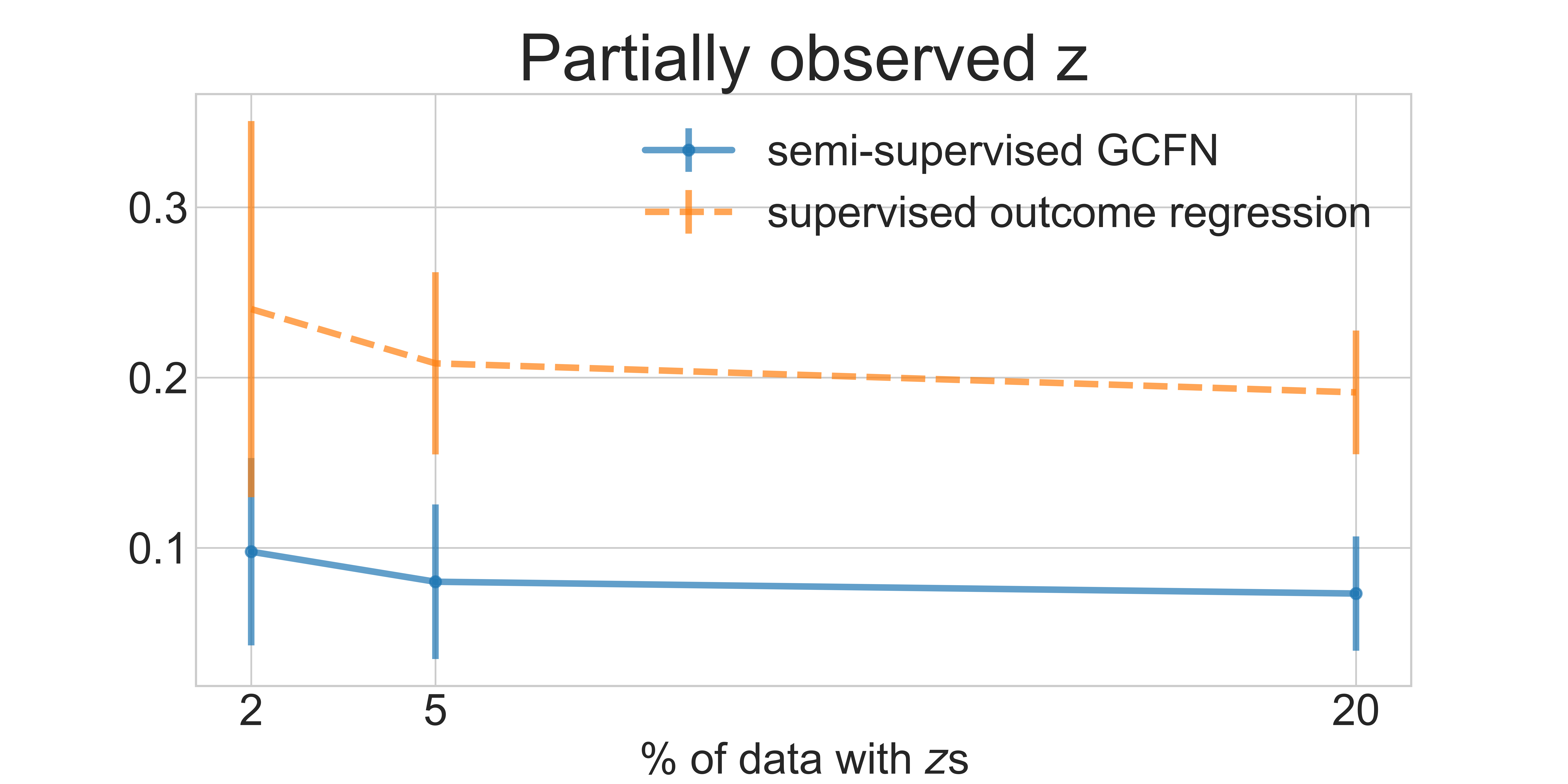
Figure 4: Mean RMSE of causal effects of the GCFN-predicted causal effects versus percentages of samples with 𝐳\boldsymbol{\mathbf{z}} observed.
Multiplicative outcome & Additive treatment

With 𝒩\mathcal{N} as the normal distribution, we generate 𝐳,ϵ∼𝒩⁡(0,1),𝐭=(𝐳+ϵ)/2,𝐲∼𝒩⁡(𝐭+α​𝐭2​𝐳,0.1),\,\,\boldsymbol{\mathbf{z}},\boldsymbol{\mathbf{\epsilon}}\sim\mathcal{N}(0,1),\,\,\boldsymbol{\mathbf{t}}=(\boldsymbol{\mathbf{z}}+\boldsymbol{\mathbf{\epsilon}})/\sqrt{2},\,\,\boldsymbol{\mathbf{y}}\sim\mathcal{N}(\boldsymbol{\mathbf{t}}+\alpha\boldsymbol{\mathbf{t}}^{2}\boldsymbol{\mathbf{z}},0.1),\, wher α\alpha controls confounding; larger magnitude of α\alpha means more confounding. The generation process above violates the linear noise relation assumption, 𝔼⁡[𝜼𝐲|𝜼𝐭]∝𝜼𝐭\mathbb{E}[\boldsymbol{\mathbf{\eta}}_{\boldsymbol{\mathbf{y}}}|\boldsymbol{\mathbf{\eta}}_{\boldsymbol{\mathbf{t}}}]\propto\boldsymbol{\mathbf{\eta}}_{\boldsymbol{\mathbf{t}}}, that CFN requires [16]. GCFN, on the other hand, does not require this assumption. In this experiment, VDE has an additive decoder which specifies a Gaussian reconstruction likelihood: 𝐭∼𝒩⁡(hϕ′​(𝐳^)+gϕ′​(ϵ),1){\boldsymbol{\mathbf{t}}}\sim\mathcal{N}(h^{\prime}_{\phi}(\hat{\boldsymbol{\mathbf{z}}})+g^{\prime}_{\phi}(\boldsymbol{\mathbf{\epsilon}}),1). In Figure 4, we compare GCFN to CFN and DeepIV, and show that GCFN produces the best causal effect estimates. Unlike the others, GCFN can adjust for confounding when the outcome process is not additive. Averaged over all α\alphas, GCFN outperforms the baselines with an RMSE of 0.09±0.06\boldsymbol{0.09\pm 0.06} compared to CFN’s 0.58±0.01\boldsymbol{0.58\pm 0.01}, 2SLS’s 0.55±0.58\boldsymbol{0.55\pm 0.58}, and DeepIV’s 0.25±0.17\boldsymbol{0.25\pm 0.17}.

Multiplicative treatment & Additive outcome.

For this simulation, we generate data as follows: 𝐳,ϵ∼𝒩⁡(0,1),𝐭=𝐳​ϵ,𝐲∼𝒩⁡(𝐭+α​𝐳,0.1).\,\,\boldsymbol{\mathbf{z}},\boldsymbol{\mathbf{\epsilon}}\sim\mathcal{N}(0,1),\,\,\boldsymbol{\mathbf{t}}=\boldsymbol{\mathbf{z}}\boldsymbol{\mathbf{\epsilon}},\,\,\boldsymbol{\mathbf{y}}\sim\mathcal{N}(\boldsymbol{\mathbf{t}}+\alpha\boldsymbol{\mathbf{z}},0.1). In this experiment, VDE has a multiplicative decoder which specifies a gaussian reconstruction likelihood with 𝐭=𝒩⁡(hϕ′​(𝐳^)​gϕ′​(ϵ),1)\boldsymbol{\mathbf{t}}=\mathcal{N}(h^{\prime}_{\phi}(\hat{\boldsymbol{\mathbf{z}}})g^{\prime}_{\phi}(\boldsymbol{\mathbf{\epsilon}}),1). The 2SLS method uses a linear model 𝐭=β​ϵ+𝜼𝐭\boldsymbol{\mathbf{t}}=\beta\boldsymbol{\mathbf{\epsilon}}+\boldsymbol{\mathbf{\eta}}_{\boldsymbol{\mathbf{t}}} which will correctly estimate 𝔼⁡[𝐭|ϵ]=0\mathbb{E}[\boldsymbol{\mathbf{t}}~|~\boldsymbol{\mathbf{\epsilon}}]=0 in our generation process. Figure 4 shows that GCFN out-performs CFN and DeepIV and is robust to different strengths of confounding (α∈{0.5,1,2}\alpha\in\{0.5,1,2\}). Averaged over all α\alphas, GCFN outperforms the baselines with an RMSE of 0.13±0.08\boldsymbol{0.13\pm 0.08} compared to CFN’s 0.58±0.02\boldsymbol{0.58\pm 0.02}, 2SLS’s 0.55±0.56\boldsymbol{0.55\pm 0.56}, and DeepIV’s 0.58±0.01\boldsymbol{0.58\pm 0.01}. We omit 2SLS from fig. 4 because it performs strictly worse than DeepIV, its deep variant. DeepIV gives effect-estimates that are close to 00. We justify this in section A.11.

4.2 GCFN with confounders observed on a subset

In this experiment, we demonstrate that semi-supervised GCFN does not need outcome or treatment process assumptions if the confounder 𝐳\boldsymbol{\mathbf{z}} is observed on a subset of the data. Let ρ\rho be the fraction with 𝐳\boldsymbol{\mathbf{z}} observed and ℬ\mathcal{B} be the Bernoulli distribution. We generate a mask 𝐦∼ℬ⁡(ρ)\boldsymbol{\mathbf{m}}\sim\mathcal{B}(\rho) and data ϵ,𝐳∼𝒩⁡(0,1),𝐭=ϵ​𝐳,𝐲∼𝒩⁡(𝐭+𝐭𝐳,0.1).\,\,\boldsymbol{\mathbf{\epsilon}},\boldsymbol{\mathbf{z}}\sim\mathcal{N}(0,1),\quad\boldsymbol{\mathbf{t}}=\boldsymbol{\mathbf{\epsilon}}\boldsymbol{\mathbf{z}},\quad\,\boldsymbol{\mathbf{y}}\sim\mathcal{N}(\boldsymbol{\mathbf{t}}+\boldsymbol{\mathbf{t}}\boldsymbol{\mathbf{z}},0.1). Let 𝐳′=𝐳∗𝐦\boldsymbol{\mathbf{z}}^{\prime}=\boldsymbol{\mathbf{z}}*\boldsymbol{\mathbf{m}}. We observe (𝐲,𝐭,ϵ,𝐳′,𝐦)(\boldsymbol{\mathbf{y}},\boldsymbol{\mathbf{t}},\boldsymbol{\mathbf{\epsilon}},\boldsymbol{\mathbf{z}}^{\prime},\boldsymbol{\mathbf{m}}). The structurally unrestricted decoder uses a categorical reconstruction likelihood: pϕ​(𝐭=j|𝐳^=z,ϵ=ϵ)∝exp⁡(gϕ​(z,ϵ,j))p_{\phi}(\boldsymbol{\mathbf{t}}=j~|~\hat{\boldsymbol{\mathbf{z}}}=z,\boldsymbol{\mathbf{\epsilon}}=\epsilon)\propto\exp{(g_{\phi}(z,\epsilon,j))}. The treatment 𝐭\boldsymbol{\mathbf{t}} is discretized into 5050 bins. The intervals [−∞,−3.5][-\infty,-3.5] and [3.5,∞][3.5,\infty] correspond to one bin each and the interval [−3.5,3.5][-3.5,3.5] is split into 48 equally-sized bins. This suffices because few samples fall outside [−3.5,3.5][-3.5,3.5]. For semi-supervised GCFN, VDE’s objective has an additional term defined on the samples with observed 𝐳\boldsymbol{\mathbf{z}}’s (eq. 8). The confounder 𝐳\boldsymbol{\mathbf{z}} is split into bins the same way as the treatment. The additional term for the it​hi^{th} sample is the categorical log-likelihood of the observed (ti,ϵi,zi)(t_{i},\epsilon_{i},z_{i}) with respect to the encoder-specified distribution: q⁡(𝐳^=zi|𝐭=ti,ϵ=ϵi)∝exp⁡(fθ​(ti,ϵi,zi))q(\hat{\boldsymbol{\mathbf{z}}}=z_{i}~|~\boldsymbol{\mathbf{t}}=t_{i},\boldsymbol{\mathbf{\epsilon}}=\epsilon_{i})\propto\exp(f_{\theta}(t_{i},\epsilon_{i},z_{i})). We set the scaling ζ\zeta on this additional term to be 0.50.5. We report results for κ=0.1\kappa=0.1. For other κ∈{0.2,0.3}\kappa\in\{0.2,0.3\}, results were similar or better.

We compare semi-supervised GCFN against regression with the same outcome model as the baseline, trained only on samples with the confounder observed. We estimated this “supervised” baseline in the same manner as the outcome stage of GCFN. Figure 4 plots the RMSE of the predicted causal effects vs. percentage of samples with observed 𝐳\boldsymbol{\mathbf{z}}’s in fig. 4. If the data has 2%2\% or more samples with the confounder observed, GCFN estimates effects better than the supervised baseline.

4.3 GCFN on high-dimensional Covariates

In this experiment, we evaluate GCFN on a non-linear simulation given in Hartford et al., 2017 to demonstrate that DeepIV improves upon 2SLS. Their generation models the effect of price (𝐭\boldsymbol{\mathbf{t}}) on sales (𝐲\boldsymbol{\mathbf{y}}), given customer covariates (𝐱\boldsymbol{\mathbf{x}}, MNIST image), and time ss; they use fuel price as an IV. The outcome is generated using the label of the MNIST image, which denotes customer price sensitivity. The data generation process for 𝐭\boldsymbol{\mathbf{t}} is additive in IV and confounder. Following this, we use the same additive decoder in VDE as in section 4.1, but with time ss as an additional input. We give further experimental details and Hartford et al., 2017’s data generating process in section B.3.

We report effect MSE on a fixed out-of-sample set (oos). We compare against Hartford et al., 2017’s reported results for two sample sizes, 10,00010,000 and 20,00020,000. DeepIV’s reported results exclude a few large effect MSE outliers; we do not exclude such errors for GCFN. We report GCFN’s performance over 1010 seeds. Overall, GCFN performed on par or better than DeepIV. First, we report GCFN’s effect MSE with κ=0.2\kappa=0.2. For 10,00010,000 samples, GCFN produced effect MSEs that ranged in [0.30−0.42][\boldsymbol{0.30-0.42}], better than DeepIV’s reported range of around [0.30−0.50][\boldsymbol{0.30-0.50}] (which is almost twice as large). For 20,00020,000 samples, GCFN’s effect MSE range improved to [0.25−0.40][\boldsymbol{0.25-0.40}] while DeepIV reported a performance of around [0.25−0.45][\boldsymbol{0.25-0.45}]. For both sample sizes, we note that κ=0.1,0.3\kappa=0.1,0.3 gave similar results. To see this, for 20,00020,000 samples, averaged over 1010 seeds, GCFN achieved a mean effect MSE of 0.305\boldsymbol{0.305} or better for any κ∈{0.1,0.2,0.3}\kappa\in\{0.1,0.2,0.3\}, beating DeepIV’s 0.32\boldsymbol{0.32}.

4.4 GCFN on high-dimensional IVs

In this experiment, we evaluate GCFN on data with a high-dimensional IV. Bennett et al., 2019 use the following data generating process to demonstrate DeepGMM [7] improves upon existing methods: ϵ∼𝒰⁡[−3,3]𝐳∼𝒩⁡(0,1)𝐭∼𝒩⁡(𝐳+ϵ,0.1)𝐲=𝒩⁡(|𝐭|+𝐳,0.1).\,\,\boldsymbol{\mathbf{\epsilon}}\sim\mathcal{U}[-3,3]\quad\boldsymbol{\mathbf{z}}\sim\mathcal{N}(0,1)\quad\boldsymbol{\mathbf{t}}\sim\mathcal{N}(\boldsymbol{\mathbf{z}}+\boldsymbol{\mathbf{\epsilon}},0.1)\quad\boldsymbol{\mathbf{y}}=\mathcal{N}\left(|\boldsymbol{\mathbf{t}}|+\boldsymbol{\mathbf{z}},0.1\right). However, the scalar ϵ\boldsymbol{\mathbf{\epsilon}} is not directly observed. Instead, ϵ\boldsymbol{\mathbf{\epsilon}} is mapped to a digit {0,…,9}\{0,\ldots,9\} and a corresponding MNIST image ϵM\boldsymbol{\mathbf{\epsilon}}_{M} is given as the IV. To estimate effects well with such an IV, any method must learn to label the MNIST image. In this setting, VDE’s encoder and decoder both take an embedding ℓγ​(ϵM)∈ℝ10\ell_{\gamma}(\boldsymbol{\mathbf{\epsilon}}_{M})\in\mathbb{R}^{10} as input. The embedding ℓγ\ell_{\gamma} is trained in VDE along with the encoder and decoder. Respecting the additive treatment process, we specify an additive decoder.

We ran GCFN with 1010 different random seeds and report results for κ=0.3\kappa=0.3, chosen based on mean test outcome MSE (OPEN0.136±0.008)0.136\pm 0.008). GCFN performs competitively with an effect MSE of 0.077±0.022\boldsymbol{0.077\pm 0.022} compared to DeepGMM’s 0.07±0.02\boldsymbol{0.07\pm 0.02} and DeepIV’s 0.11±0.00\boldsymbol{0.11\pm 0.00}, both as reported in [7]. Effect MSE for κ∈{0.2,0.4}\kappa\in\{0.2,0.4\} were similar and within standard error of DeepGMM’s performance. See section B.4 for further experimental details and results.

4.5 The Effect of Slave Export on Trust

We demonstrate the recovery of the causal effect of slave export on the trust in the community [30]. Nunn and Wantchekon, 2011 pooled surveys and historical records to get sub-ethnicity and tribe level data from the period of slave trade. The data was used to study the long-term effects of slave-trade, measured in the 2005 Afrobarometer survey. We predict the effect of the treatment 𝐭=\boldsymbol{\mathbf{t}}=ln(1 + slave-export/area) on the outcome of interest, 𝐲=\boldsymbol{\mathbf{y}}=trust in neighbors. The dataset has 69326932 samples with 5959 features. After filtering out missing values, we preprocessed 4646 covariates and IV to have mean 00 and maximum 11, and the treatment 𝐭\boldsymbol{\mathbf{t}} to lie in [0,2][0,2]. The authors claim that the distance to sea cannot causally affect how individuals trust each other, but it affects the chance of coming in contact with colonial slave-traders and being shipped to the Americas, making it an IV. They control for urbanization, fixed effects for sophistication, political hierarchies beyond community, integration with the rail network, contact with European explorers, and missions during colonial rule.

For this experiment, VDE’s decoder gϕg_{\phi} specifies a categorical reconstruction likelihood as pϕ​(𝐭=i|𝐳^=z,ϵ=ϵ)∝exp⁡(gϕ​(z,ϵ,i))p_{\phi}(\boldsymbol{\mathbf{t}}=i~|~\hat{\boldsymbol{\mathbf{z}}}=z,\boldsymbol{\mathbf{\epsilon}}=\epsilon)\propto\exp{(g_{\phi}(z,\epsilon,i))}. Each category of the treatment corresponds to one of 50 equally-sized bins in the interval [0,2][0,2]. Nunn and Wantchekon, 2011 use a linear model for the outcome 𝐲\boldsymbol{\mathbf{y}} and use the distance to sea as an IV for each community. We also use a partially linear model 𝐲=β​𝐭+hθ​(𝐳^)\boldsymbol{\mathbf{y}}=\beta\boldsymbol{\mathbf{t}}+h_{\theta}(\hat{\boldsymbol{\mathbf{z}}}) so that the effect we recover is of comparable nature to the effect reported in the paper. The outcome network hθh_{\theta} has 2 layers with 10 hidden units each and ReLUs.

Averaged over 44 mutual information coefficients κ\kappa and 55 random seeds, GCFN’s estimate of β\beta was −0.21±0.04\boldsymbol{-0.21\pm 0.04} compared with −0.27±0.10\boldsymbol{-0.27\pm 0.10}, as reported by Nunn and Wantchekon, 2011.

5 Discussion and Future

In this paper, we characterize general control functions for causal estimation. General control functions allow for effect estimation without structural outcome process assumptions like 2SLS or CFN. The key challenge in building general control functions is ensuring joint independence between the IV and the control function and (unobserved) true confounder. Joint independence can be guaranteed via structural treatment process assumptions, like additivity or monotonicity. We develop the general control function method (GCFN) to build general control functions and estimate effects with them. Further, we develop semi-supervised GCFN which uses confounders observed on a subset of the data to construct general control functions without treatment process assumptions. Finally, we consider imperfect estimation of the general control function and bound average error in effects using quantities optimized in VDE.

Tradeoffs with assumptions.

In causal estimation, parametric assumptions can be traded-off with assumptions of strength of IV or positivity. Consider a setting where ϵ\boldsymbol{\mathbf{\epsilon}} is binary. For every possible confounder value, only two values of the treatment are observed. Thus it is impossible to estimate a quadratic function of 𝐭\boldsymbol{\mathbf{t}} for each fixed value of the confounder. This means 𝐲|𝐭\boldsymbol{\mathbf{y}}~|~\boldsymbol{\mathbf{t}} is not identified without strong assumptions like linearity in 𝐭\boldsymbol{\mathbf{t}}. Incorporating outcome properties, like the conditional independence 𝐲⊧ϵ|𝐭,𝐳\boldsymbol{\mathbf{y}}\rotatebox[origin]{90.0}{$\models$}\boldsymbol{\mathbf{\epsilon}}~|~\boldsymbol{\mathbf{t}},\boldsymbol{\mathbf{z}}, into control function estimation would be a fruitful direction.

Broader Impact

Our work applies to causal inference where strong IVs are available to help adjust for confounding, such as in problems in healthcare and economics. We assess the impact of our work in the context of these fields. In general, loosening functional assumptions like GCFN does, helps estimate effects better. Better effect estimates help improve planning patient treatment and understanding policy impact. However, the strong IV assumption may not hold for all demographics. If this occurs, demographics for which the assumption holds will have better quality effect estimates than for demographics where the assumption does not hold. This could mean that certain demographics receive better care in hospitals or have implemented policy be more impactful on them. Such issues could be characterized by evaluating the positivity of treatment with respect to the constructed control function in different demographics.

Acknowledgements

The authors were partly supported by NIH/NHLBI Award R01HL148248, and by NSF Award 1922658 NRT-HDR: FUTURE Foundations, Translation, and Responsibility for Data Science. The authors would like to thank Xintian Han and the reviewers for thoughtful feedback.

References

  • Agakov and Barber, [2004] Agakov, F. V. and Barber, D. (2004). An auxiliary variational method. In International Conference on Neural Information Processing, pages 561–566. Springer.
  • Amemiya, [1974] Amemiya, T. (1974). The nonlinear two-stage least-squares estimator. Journal of econometrics, 2(2):105–110.
  • Angrist et al., [1996] Angrist, J. D., Imbens, G. W., and Rubin, D. B. (1996). Identification of causal effects using instrumental variables. Journal of the American statistical Association, 91(434):444–455.
  • Angrist and Krueger, [2001] Angrist, J. D. and Krueger, A. B. (2001). Instrumental variables and the search for identification: From supply and demand to natural experiments. Journal of Economic perspectives, 15(4):69–85.
  • Baker et al., [1999] Baker, M., Benjamin, D., and Stanger, S. (1999). The highs and lows of the minimum wage effect: A time-series cross-section study of the canadian law. Journal of Labor Economics, 17(2):318–350.
  • Balke and Pearl, [1997] Balke, A. and Pearl, J. (1997). Bounds on treatment effects from studies with imperfect compliance. Journal of the American Statistical Association, 92(439):1171–1176.
  • Bennett et al., [2019] Bennett, A., Kallus, N., and Schnabel, T. (2019). Deep generalized method of moments for instrumental variable analysis. arXiv preprint arXiv:1905.12495.
  • Card, [1993] Card, D. (1993). Using geographic variation in college proximity to estimate the return to schooling. Technical report, National Bureau of Economic Research.
  • Chesher, [2003] Chesher, A. (2003). Identification in nonseparable models. Econometrica, 71(5):1405–1441.
  • Chetverikov and Wilhelm, [2017] Chetverikov, D. and Wilhelm, D. (2017). Nonparametric instrumental variable estimation under monotonicity. Econometrica, 85(4):1303–1320.
  • Cunha et al., [2010] Cunha, F., Heckman, J. J., and Schennach, S. M. (2010). Estimating the technology of cognitive and noncognitive skill formation. Econometrica, 78(3):883–931.
  • Darolles et al., [2011] Darolles, S., Fan, Y., Florens, J.-P., and Renault, E. (2011). Nonparametric instrumental regression. Econometrica, 79(5):1541–1565.
  • Dehejia and Wahba, [2002] Dehejia, R. H. and Wahba, S. (2002). Propensity score-matching methods for nonexperimental causal studies. Review of Economics and statistics, 84(1):151–161.
  • Funk et al., [2011] Funk, M. J., Westreich, D., Wiesen, C., Stürmer, T., Brookhart, M. A., and Davidian, M. (2011). Doubly robust estimation of causal effects. American journal of epidemiology, 173(7):761–767.
  • Glasserman, [2013] Glasserman, P. (2013). Monte Carlo methods in financial engineering, volume 53. Springer Science & Business Media.
  • Guo and Small, [2016] Guo, Z. and Small, D. S. (2016). Control function instrumental variable estimation of nonlinear causal effect models. The Journal of Machine Learning Research, 17(1):3448–3482.
  • Hansen, [1982] Hansen, L. P. (1982). Large sample properties of generalized method of moments estimators. Econometrica: Journal of the Econometric Society, pages 1029–1054.
  • Hartford et al., [2017] Hartford, J., Lewis, G., Leyton-Brown, K., and Taddy, M. (2017). Deep iv: A flexible approach for counterfactual prediction. In Proceedings of the 34th International Conference on Machine Learning-Volume 70, pages 1414–1423. JMLR. org.
  • Heckman and Robb Jr, [1985] Heckman, J. J. and Robb Jr, R. (1985). Alternative methods for evaluating the impact of interventions: An overview. Journal of econometrics, 30(1-2):239–267.
  • Imbens and Newey, [2009] Imbens, G. W. and Newey, W. K. (2009). Identification and estimation of triangular simultaneous equations models without additivity. Econometrica, 77(5):1481–1512.
  • Kelejian, [1971] Kelejian, H. H. (1971). Two-stage least squares and econometric systems linear in parameters but nonlinear in the endogenous variables. Journal of the American Statistical Association, 66(334):373–374.
  • Kingma and Ba, [2014] Kingma, D. P. and Ba, J. (2014). Adam: A method for stochastic optimization. arXiv preprint arXiv:1412.6980.
  • Lieberson, [1987] Lieberson, S. (1987). Making it count: The improvement of social research and theory. Univ of California Press.
  • Maaløe et al., [2016] Maaløe, L., Sønderby, C. K., Sønderby, S. K., and Winther, O. (2016). Auxiliary deep generative models. arXiv preprint arXiv:1602.05473.
  • Manski, [1990] Manski, C. F. (1990). Nonparametric bounds on treatment effects. The American Economic Review, 80(2):319–323.
  • McGue et al., [2010] McGue, M., Osler, M., and Christensen, K. (2010). Causal inference and observational research: The utility of twins. Perspectives on psychological science, 5(5):546–556.
  • Mnih and Gregor, [2014] Mnih, A. and Gregor, K. (2014). Neural variational inference and learning in belief networks. arXiv preprint arXiv:1402.0030.
  • Newey, [2013] Newey, W. K. (2013). Nonparametric instrumental variables estimation. American Economic Review, 103(3):550–56.
  • Niles-Weed and Rigollet, [2019] Niles-Weed, J. and Rigollet, P. (2019). Estimation of wasserstein distances in the spiked transport model. arXiv preprint arXiv:1909.07513.
  • Nunn and Wantchekon, [2011] Nunn, N. and Wantchekon, L. (2011). The slave trade and the origins of mistrust in africa. American Economic Review, 101(7):3221–52.
  • Pearl et al., [2009] Pearl, J. et al. (2009). Causal inference in statistics: An overview. Statistics surveys, 3:96–146.
  • Ranganath et al., [2014] Ranganath, R., Gerrish, S., and Blei, D. (2014). Black box variational inference. In Artificial Intelligence and Statistics, pages 814–822.
  • Ranganath and Perotte, [2018] Ranganath, R. and Perotte, A. (2018). Multiple causal inference with latent confounding. arXiv preprint arXiv:1805.08273.
  • Ranganath et al., [2016] Ranganath, R., Tran, D., and Blei, D. (2016). Hierarchical variational models. In International Conference on Machine Learning, pages 324–333.
  • Rothman and Greenland, [2005] Rothman, K. J. and Greenland, S. (2005). Causation and causal inference in epidemiology. American journal of public health, 95(S1):S144–S150.
  • Salimans et al., [2014] Salimans, T., Kingma, D. P., and Welling, M. (2014). Markov chain monte carlo and variational inference: Bridging the gap. arXiv preprint arXiv:1410.6460.
  • Seabold and Perktold, [2010] Seabold, S. and Perktold, J. (2010). statsmodels: Econometric and statistical modeling with python. In 9th Python in Science Conference.
  • Shalit et al., [2017] Shalit, U., Johansson, F. D., and Sontag, D. (2017). Estimating individual treatment effect: generalization bounds and algorithms. In Proceedings of the 34th International Conference on Machine Learning-Volume 70, pages 3076–3085. JMLR. org.
  • Singh et al., [2019] Singh, R., Sahani, M., and Gretton, A. (2019). Kernel instrumental variable regression. arXiv preprint arXiv:1906.00232.
  • Stuart et al., [2013] Stuart, E. A., DuGoff, E., Abrams, M., Salkever, D., and Steinwachs, D. (2013). Estimating causal effects in observational studies using electronic health data: challenges and (some) solutions. Egems, 1(3).
  • Wager and Athey, [2018] Wager, S. and Athey, S. (2018). Estimation and inference of heterogeneous treatment effects using random forests. Journal of the American Statistical Association, 113(523):1228–1242.
  • Wald, [1940] Wald, A. (1940). The fitting of straight lines if both variables are subject to error. The Annals of Mathematical Statistics, 11(3):284–300.
  • Wiesenfarth et al., [2014] Wiesenfarth, M., Hisgen, C. M., Kneib, T., and Cadarso-Suarez, C. (2014). Bayesian nonparametric instrumental variables regression based on penalized splines and dirichlet process mixtures. Journal of Business & Economic Statistics, 32(3):468–482.
  • Williams, [1992] Williams, R. J. (1992). Simple statistical gradient-following algorithms for connectionist reinforcement learning. Machine learning, 8(3-4):229–256.
  • Wooldridge, [2015] Wooldridge, J. M. (2015). Control function methods in applied econometrics. Journal of Human Resources, 50(2):420–445.

Supplementary Material for VDE and GCFN

Appendix A Theoretical Details and Proofs

Notation

We use the expectation operator in different contexts in the proof. 𝔼q\mathbb{E}_{q} denotes expectation with respect to the density qq and 𝔼𝐳\mathbb{E}_{\boldsymbol{\mathbf{z}}} denotes expectation with respect to the density of the random variable 𝐳\boldsymbol{\mathbf{z}}. When the density function or the random variable are clear from the context, we drop the subscript and use 𝔼\mathbb{E}.

A.1 The general IV causal graph with covariates/observed confounders

𝐳\boldsymbol{\mathbf{z}}𝐱\boldsymbol{\mathbf{x}}ϵ\boldsymbol{\mathbf{\epsilon}}𝐭\boldsymbol{\mathbf{t}}𝐲\boldsymbol{\mathbf{y}}
Figure 5: Causal graph with hidden confounder 𝐳\boldsymbol{\mathbf{z}}, outcome 𝐲\boldsymbol{\mathbf{y}}, IV ϵ\boldsymbol{\mathbf{\epsilon}}, treatment 𝐭\boldsymbol{\mathbf{t}} and covariates 𝐱\boldsymbol{\mathbf{x}}.

Figure 5 is the general version of the IV problem where the instrumental variable property holds true after conditioning on 𝐱\boldsymbol{\mathbf{x}}. This is sometimes called a conditional instrument. All our proofs and results carry over to the situation with covariates after conditioning all estimables and distributions on 𝐱\boldsymbol{\mathbf{x}}. VDE in this setting with covariates is re-written as:

maxθ,ϕ\displaystyle\max_{\theta,\phi} 𝔼F⁡(𝐭,ϵ,𝐱)​𝔼qθ​(𝐳^|𝐭,ϵ,𝐱)​log⁡pϕ​(𝐭|𝐳^,ϵ,𝐱)−λ​𝐈θ​(𝐳^;ϵ|𝐱)\displaystyle\,\mathbb{E}_{F(\boldsymbol{\mathbf{t}},\boldsymbol{\mathbf{\epsilon}},\boldsymbol{\mathbf{x}})}\mathbb{E}_{q_{\theta}(\hat{\boldsymbol{\mathbf{z}}}~|~\boldsymbol{\mathbf{t}},\boldsymbol{\mathbf{\epsilon}},\boldsymbol{\mathbf{x}})}\log p_{\phi}(\boldsymbol{\mathbf{t}}~|~\hat{\boldsymbol{\mathbf{z}}},\boldsymbol{\mathbf{\epsilon}},\boldsymbol{\mathbf{x}})-\lambda\mathbf{I}_{\theta}(\hat{\boldsymbol{\mathbf{z}}};\boldsymbol{\mathbf{\epsilon}}|\boldsymbol{\mathbf{x}}) (9)

A.2 Mutual Information lower bound

Here, we show the full derivation of the lower bound for negative mutual-information. We derive the lower bound for the general case where there are both observed and unobserved confounders. A simple lower bound can be obtained by using 𝐇⁡(𝐳^|ϵ,𝐱)≥𝐇⁡(𝐳^|ϵ,𝐭,𝐱)\mathbf{H}(\hat{\boldsymbol{\mathbf{z}}}~|~\boldsymbol{\mathbf{\epsilon}},\boldsymbol{\mathbf{x}})\geq\mathbf{H}(\hat{\boldsymbol{\mathbf{z}}}~|~\boldsymbol{\mathbf{\epsilon}},\boldsymbol{\mathbf{t}},\boldsymbol{\mathbf{x}}), but this cannot be made tight unless ϵ\boldsymbol{\mathbf{\epsilon}} completely determines 𝐭\boldsymbol{\mathbf{t}}. Therefore, we cannot guarantee independence unless the data at hand is not confounded. Instead we introduce two auxiliary distributions rν​(𝐳^|𝐱)r_{\nu}(\hat{\boldsymbol{\mathbf{z}}}~|~\boldsymbol{\mathbf{x}}) and pϕ​(𝐭|ϵ,𝐳^,𝐱)p_{\phi}(\boldsymbol{\mathbf{t}}~|~\boldsymbol{\mathbf{\epsilon}},\hat{\boldsymbol{\mathbf{z}}},\boldsymbol{\mathbf{x}}), following the work in variational inference  [34, 1, 36, 24] and causal inference [33].

We let F⁡(𝐭,𝐱,ϵ,𝐲)F(\boldsymbol{\mathbf{t}},\boldsymbol{\mathbf{x}},\boldsymbol{\mathbf{\epsilon}},\boldsymbol{\mathbf{y}}) be the true data distribution and qθ​(𝐳^|𝐭,ϵ,𝐱=x)q_{\theta}(\hat{\boldsymbol{\mathbf{z}}}~|~\boldsymbol{\mathbf{t}},\boldsymbol{\mathbf{\epsilon}},\boldsymbol{\mathbf{x}}=x) be the control function distribution. We overload notation and also use qθq_{\theta} to refer to any distribution that involves operations with qθ​(𝐳^|𝐭,ϵ,𝐱=x)q_{\theta}(\hat{\boldsymbol{\mathbf{z}}}~|~\boldsymbol{\mathbf{t}},\boldsymbol{\mathbf{\epsilon}},\boldsymbol{\mathbf{x}}=x). We use =c\mathrel{\overset{\makebox[0.0pt]{\mbox{\tiny c}}}{=}} to denote that the LHS and RHS are equal up to constants that are ignored during optimization. In the following, both 𝐇⁡(𝐭,ϵ|𝐱=x)\mathbf{H}(\boldsymbol{\mathbf{t}},\boldsymbol{\mathbf{\epsilon}}~|~\boldsymbol{\mathbf{x}}=x), 𝐇⁡(ϵ|𝐱=x)\mathbf{H}(\boldsymbol{\mathbf{\epsilon}}|\boldsymbol{\mathbf{x}}=x) are constants with respect to the parameters of interest ϕ,θ,ν\phi,\theta,\nu and we will drop them from the lower bound when encountered. For a given 𝐱=x\boldsymbol{\mathbf{x}}=x, we lower-bound the negative instantaneous conditional mutual information:

−λ\displaystyle-\lambda 𝐈(𝐳^;ϵ|x)=−λKL(qθ(𝐳^,ϵ|x)∥qθ(𝐳^|x)F(ϵ|x))\displaystyle\mathbf{I}(\hat{\boldsymbol{\mathbf{z}}};\boldsymbol{\mathbf{\epsilon}}~|~x)=-\lambda\textrm{KL}\left(q_{\theta}(\hat{\boldsymbol{\mathbf{z}}},\boldsymbol{\mathbf{\epsilon}}~|~x)\;\|\;q_{\theta}(\hat{\boldsymbol{\mathbf{z}}}~|~x)F(\boldsymbol{\mathbf{\epsilon}}~|~x)\right)
=\displaystyle= −λ⁡[𝔼qθ​(ϵ,𝐳^|x)​[log⁡qθ​(ϵ|𝐳^,x)−log⁡F⁡(ϵ|x)]]\displaystyle-\lambda\left[\mathbb{E}_{q_{\theta}(\boldsymbol{\mathbf{\epsilon}},\hat{\boldsymbol{\mathbf{z}}}~|~x)}\left[\log q_{\theta}(\boldsymbol{\mathbf{\epsilon}}~|~\hat{\boldsymbol{\mathbf{z}}},x)-\log F(\boldsymbol{\mathbf{\epsilon}}~|~x)\right]\right]
=\displaystyle= −λ⁡[𝔼qθ​(ϵ,𝐳^|x)​[log⁡qθ​(ϵ|𝐳^,x)]+𝐇⁡(ϵ|x)]\displaystyle-\lambda\left[\mathbb{E}_{q_{\theta}(\boldsymbol{\mathbf{\epsilon}},\hat{\boldsymbol{\mathbf{z}}}~|~x)}\left[\log q_{\theta}(\boldsymbol{\mathbf{\epsilon}}~|~\hat{\boldsymbol{\mathbf{z}}},x)\right]+\mathbf{H}(\boldsymbol{\mathbf{\epsilon}}~|~x)\right]
=c\displaystyle\mathrel{\overset{\makebox[0.0pt]{\mbox{\tiny c}}}{=}} −λ[𝔼qθ​(ϵ,𝐳^|x)[KL(qθ(𝐳^|x)∥qθ(𝐳^|x))+KL(qθ(𝐭|ϵ,𝐳^,x)∥qθ(𝐭|ϵ,𝐳^,x))+logqθ(ϵ|𝐳^,x)]]\displaystyle-\lambda\big[\mathbb{E}_{q_{\theta}(\boldsymbol{\mathbf{\epsilon}},\hat{\boldsymbol{\mathbf{z}}}~|~x)}\big[\textrm{KL}\left(q_{\theta}(\hat{\boldsymbol{\mathbf{z}}}~|~x)\;\|\;q_{\theta}(\hat{\boldsymbol{\mathbf{z}}}~|~x)\right)+\textrm{KL}\left(q_{\theta}(\boldsymbol{\mathbf{t}}~|~\boldsymbol{\mathbf{\epsilon}},\hat{\boldsymbol{\mathbf{z}}},x)\;\|\;q_{\theta}(\boldsymbol{\mathbf{t}}~|~\boldsymbol{\mathbf{\epsilon}},\hat{\boldsymbol{\mathbf{z}}},x)\right)+\log q_{\theta}(\boldsymbol{\mathbf{\epsilon}}~|~\hat{\boldsymbol{\mathbf{z}}},x)\big]\big]
≥\displaystyle\geq −λ[𝔼qθ​(ϵ,𝐳^|x)[KL(qθ(𝐳^|x)∥rν(𝐳^|x))+KL(qθ(𝐭|ϵ,𝐳^,x)∥pϕ(𝐭|ϵ,𝐳^,x))+logqθ(ϵ|𝐳^,x)]]\displaystyle-\lambda\big[\mathbb{E}_{q_{\theta}(\boldsymbol{\mathbf{\epsilon}},\hat{\boldsymbol{\mathbf{z}}}~|~x)}\big[\textrm{KL}\left(q_{\theta}(\hat{\boldsymbol{\mathbf{z}}}~|~x)\;\|\;r_{\nu}(\hat{\boldsymbol{\mathbf{z}}}~|~x)\right)+\textrm{KL}\left(q_{\theta}(\boldsymbol{\mathbf{t}}~|~\boldsymbol{\mathbf{\epsilon}},\hat{\boldsymbol{\mathbf{z}}},x)\;\|\;p_{\phi}(\boldsymbol{\mathbf{t}}~|~\boldsymbol{\mathbf{\epsilon}},\hat{\boldsymbol{\mathbf{z}}},x)\right)+\log q_{\theta}(\boldsymbol{\mathbf{\epsilon}}~|~\hat{\boldsymbol{\mathbf{z}}},x)\big]\big]
=\displaystyle= −λ[𝔼qθ​(ϵ,𝐳^|x)[log[qθ(𝐳^,ϵ|x)]+𝔼qθ​(𝐭|ϵ,𝐳^,x)logqθ(𝐭|ϵ,𝐳^,x)\displaystyle-\lambda\big[\mathbb{E}_{q_{\theta}(\boldsymbol{\mathbf{\epsilon}},\hat{\boldsymbol{\mathbf{z}}}~|~x)}\big[\log\left[q_{\theta}(\hat{\boldsymbol{\mathbf{z}}},\boldsymbol{\mathbf{\epsilon}}~|~x)\right]+\mathbb{E}_{q_{\theta}(\boldsymbol{\mathbf{t}}~|~\boldsymbol{\mathbf{\epsilon}},\hat{\boldsymbol{\mathbf{z}}},x)}\log q_{\theta}(\boldsymbol{\mathbf{t}}~|~\boldsymbol{\mathbf{\epsilon}},\hat{\boldsymbol{\mathbf{z}}},x)
−𝔼qθ​(𝐳^|x)logrν(𝐳^|x)−𝔼qθ​(𝐭,ϵ,𝐳^|x)logpϕ(𝐭|ϵ,𝐳^,x)]\displaystyle\quad\quad-\mathbb{E}_{q_{\theta}(\hat{\boldsymbol{\mathbf{z}}}~|~x)}\log r_{\nu}(\hat{\boldsymbol{\mathbf{z}}}~|~x)-\mathbb{E}_{q_{\theta}(\boldsymbol{\mathbf{t}},\boldsymbol{\mathbf{\epsilon}},\hat{\boldsymbol{\mathbf{z}}}~|~x)}\log p_{\phi}(\boldsymbol{\mathbf{t}}~|~\boldsymbol{\mathbf{\epsilon}},\hat{\boldsymbol{\mathbf{z}}},x)\big]
=\displaystyle= −λ⁡[𝔼qθ​(ϵ,𝐳^,𝐭|x)​log⁡[qθ​(𝐳^,ϵ,𝐭|x)]−𝔼qθ​(𝐳^|x)​log⁡rν​(𝐳^|x)−𝔼qθ​(𝐭,ϵ,𝐳^|x)​log⁡pϕ​(𝐭|ϵ,𝐳^,x)]\displaystyle-\lambda\big[\mathbb{E}_{q_{\theta}(\boldsymbol{\mathbf{\epsilon}},\hat{\boldsymbol{\mathbf{z}}},\boldsymbol{\mathbf{t}}~|~x)}\log\left[q_{\theta}(\hat{\boldsymbol{\mathbf{z}}},\boldsymbol{\mathbf{\epsilon}},\boldsymbol{\mathbf{t}}~|~x)\right]-\mathbb{E}_{q_{\theta}(\hat{\boldsymbol{\mathbf{z}}}~|~x)}\log r_{\nu}(\hat{\boldsymbol{\mathbf{z}}}~|~x)-\mathbb{E}_{q_{\theta}(\boldsymbol{\mathbf{t}},\boldsymbol{\mathbf{\epsilon}},\hat{\boldsymbol{\mathbf{z}}}~|~x)}\log p_{\phi}(\boldsymbol{\mathbf{t}}~|~\boldsymbol{\mathbf{\epsilon}},\hat{\boldsymbol{\mathbf{z}}},x)\big]
=\displaystyle= −λ[𝔼F⁡(𝐭,ϵ|x)𝔼qθ​(𝐳^|ϵ,𝐭,x)log[qθ(𝐳^|𝐭,ϵ,x)−logpϕ(𝐭|ϵ,𝐳^,x)]−𝐇(𝐭,ϵ|x)\displaystyle-\lambda\big[\mathbb{E}_{F(\boldsymbol{\mathbf{t}},\boldsymbol{\mathbf{\epsilon}}~|~x)}\mathbb{E}_{q_{\theta}(\hat{\boldsymbol{\mathbf{z}}}~|~\boldsymbol{\mathbf{\epsilon}},\boldsymbol{\mathbf{t}},x)}\log\left[q_{\theta}(\hat{\boldsymbol{\mathbf{z}}}~|~\boldsymbol{\mathbf{t}},\boldsymbol{\mathbf{\epsilon}},x)-\log p_{\phi}(\boldsymbol{\mathbf{t}}~|~\boldsymbol{\mathbf{\epsilon}},\hat{\boldsymbol{\mathbf{z}}},x)\right]-\mathbf{H}(\boldsymbol{\mathbf{t}},\boldsymbol{\mathbf{\epsilon}}~|~x)
−𝔼qθ​(𝐳^|x)logrν(𝐳^|x)]\displaystyle\quad\quad-\mathbb{E}_{q_{\theta}(\hat{\boldsymbol{\mathbf{z}}}~|~x)}\log r_{\nu}(\hat{\boldsymbol{\mathbf{z}}}~|~x)\big]
=c\displaystyle\mathrel{\overset{\makebox[0.0pt]{\mbox{\tiny c}}}{=}} −λ𝔼F⁡(𝐭,ϵ|x)[KL(qθ(𝐳^|𝐭,ϵ,x)∥rν(𝐳^|x))−𝔼qθ​(𝐳^|ϵ,𝐭,x)logpϕ(𝐭|ϵ,𝐳^,x)],\displaystyle-\lambda\mathbb{E}_{F(\boldsymbol{\mathbf{t}},\boldsymbol{\mathbf{\epsilon}}~|~x)}\left[\textrm{KL}\left(q_{\theta}(\hat{\boldsymbol{\mathbf{z}}}~|~\boldsymbol{\mathbf{t}},\boldsymbol{\mathbf{\epsilon}},x)\;\|\;r_{\nu}(\hat{\boldsymbol{\mathbf{z}}}~|~x)\right)-\mathbb{E}_{q_{\theta}(\hat{\boldsymbol{\mathbf{z}}}~|~\boldsymbol{\mathbf{\epsilon}},\boldsymbol{\mathbf{t}},x)}\log p_{\phi}(\boldsymbol{\mathbf{t}}~|~\boldsymbol{\mathbf{\epsilon}},\hat{\boldsymbol{\mathbf{z}}},x)\right],

where the hidden term −λ⁡[𝐇⁡(ϵ|𝐱=x)−𝐇⁡(𝐭,ϵ|𝐱=x)]-\lambda\left[\mathbf{H}(\boldsymbol{\mathbf{\epsilon}}~|~\boldsymbol{\mathbf{x}}=x)-\mathbf{H}(\boldsymbol{\mathbf{t}},\boldsymbol{\mathbf{\epsilon}}~|~\boldsymbol{\mathbf{x}}=x)\right] is a constant for a given instance of the problem. We do not need access to the distribution 𝐭,𝐳^,ϵ|𝐱=x\boldsymbol{\mathbf{t}},\hat{\boldsymbol{\mathbf{z}}},\boldsymbol{\mathbf{\epsilon}}~|~\boldsymbol{\mathbf{x}}=x because the information that we lower bounded, 𝐈⁡(𝐳^;ϵ|𝐱=x)\mathbf{I}(\hat{\boldsymbol{\mathbf{z}}};\boldsymbol{\mathbf{\epsilon}}~|~\boldsymbol{\mathbf{x}}=x), is averaged over 𝐱=x\boldsymbol{\mathbf{x}}=x in our objective. Recall that pϕ​(𝐭|ϵ,𝐳^,𝐱=x)p_{\phi}(\boldsymbol{\mathbf{t}}~|~\boldsymbol{\mathbf{\epsilon}},\hat{\boldsymbol{\mathbf{z}}},\boldsymbol{\mathbf{x}}=x) is the reconstruction term in VDE. This lower bound is tight when the introduced KL terms are 0, which occurs when rν​(𝐳^|𝐱=x)=qθ​(𝐳^|𝐱=x)r_{\nu}(\hat{\boldsymbol{\mathbf{z}}}~|~\boldsymbol{\mathbf{x}}=x)=q_{\theta}(\hat{\boldsymbol{\mathbf{z}}}~|~\boldsymbol{\mathbf{x}}=x) and pϕ​(𝐭|ϵ,𝐱=x,𝐳^)=qθ​(𝐭|ϵ,𝐱=x,𝐳^)p_{\phi}(\boldsymbol{\mathbf{t}}~|~\boldsymbol{\mathbf{\epsilon}},\boldsymbol{\mathbf{x}}=x,\hat{\boldsymbol{\mathbf{z}}})=q_{\theta}(\boldsymbol{\mathbf{t}}~|~\boldsymbol{\mathbf{\epsilon}},\boldsymbol{\mathbf{x}}=x,\hat{\boldsymbol{\mathbf{z}}}). This means that if the models pϕ,rνp_{\phi},r_{\nu} are rich enough, the gap between the lower bound and mutual information can be optimized to be zero. The second term 𝔼qθ​(𝐳^|ϵ,𝐭,𝐱=x)​log⁡pϕ​(𝐭|ϵ,𝐳^,𝐱=x)\mathbb{E}_{q_{\theta}(\hat{\boldsymbol{\mathbf{z}}}~|~\boldsymbol{\mathbf{\epsilon}},\boldsymbol{\mathbf{t}},\boldsymbol{\mathbf{x}}=x)}\log p_{\phi}(\boldsymbol{\mathbf{t}}~|~\boldsymbol{\mathbf{\epsilon}},\hat{\boldsymbol{\mathbf{z}}},\boldsymbol{\mathbf{x}}=x) is the same as the reconstruction likelihood. Thus substituting the lower bound into the full objective with given covariates gives

𝔼F⁡(𝐭,ϵ,𝐱)[(1+λ)𝔼qθ​(𝐳^|𝐭,ϵ,𝐱)logpϕ(𝐭|ϵ,𝐳^,𝐱)−λKL(qθ(𝐳^|𝐭,ϵ,𝐱)∥rν(𝐳^|𝐱))]\displaystyle\mathbb{E}_{F(\boldsymbol{\mathbf{t}},\boldsymbol{\mathbf{\epsilon}},\boldsymbol{\mathbf{x}})}\left[(1+\lambda)\mathbb{E}_{q_{\theta}(\hat{\boldsymbol{\mathbf{z}}}~|~\boldsymbol{\mathbf{t}},\boldsymbol{\mathbf{\epsilon}},\boldsymbol{\mathbf{x}})}\log p_{\phi}(\boldsymbol{\mathbf{t}}~|~\boldsymbol{\mathbf{\epsilon}},\hat{\boldsymbol{\mathbf{z}}},\boldsymbol{\mathbf{x}})-\lambda\textrm{KL}\left(q_{\theta}(\hat{\boldsymbol{\mathbf{z}}}~|~\boldsymbol{\mathbf{t}},\boldsymbol{\mathbf{\epsilon}},\boldsymbol{\mathbf{x}})\;\|\;r_{\nu}(\hat{\boldsymbol{\mathbf{z}}}~|~\boldsymbol{\mathbf{x}})\right)\right]
Optimization for variational decoupling (VDE).

The VDE optimization involves the expectations of distributions with parameters with respect to a distribution that also has parameters. For distributions that are not being integrated against, we can move the gradient inside the expectation. For distributions that are integrated against, score-function methods provide a general tool to compute stochastic gradients; Glasserman, 2013, Williams, 1992, Ranganath et al., 2014, Mnih and Gregor, 2014. In our experiments, we let the control function be a categorical variable. This allows us to marginalize out the control function and compute the gradient.

A.3 Proof of Theorem 1

Theorem 1.

(Meta-identification result for general control functions)
Let F⁡(𝐭,ϵ,𝐲)F(\boldsymbol{\mathbf{t}},\boldsymbol{\mathbf{\epsilon}},\boldsymbol{\mathbf{y}}) be the true data distribution. Let control function 𝐳^\hat{\boldsymbol{\mathbf{z}}} be sampled conditionally on 𝐭,ϵ\boldsymbol{\mathbf{t}},\boldsymbol{\mathbf{\epsilon}}. Let q⁡(𝐳^,𝐭,ϵ)=q⁡(𝐳^|𝐭,ϵ)​F​(𝐭,ϵ)q(\hat{\boldsymbol{\mathbf{z}}},\boldsymbol{\mathbf{t}},\boldsymbol{\mathbf{\epsilon}})=q(\hat{\boldsymbol{\mathbf{z}}}~|~\boldsymbol{\mathbf{t}},\boldsymbol{\mathbf{\epsilon}})F(\boldsymbol{\mathbf{t}},\boldsymbol{\mathbf{\epsilon}}) be the joint distribution over 𝐳^,𝐭,ϵ\hat{\boldsymbol{\mathbf{z}}},\boldsymbol{\mathbf{t}},\boldsymbol{\mathbf{\epsilon}}. Further, let gg be a deterministic function and 𝛅\boldsymbol{\mathbf{\delta}} be independent noise such that 𝐭=g⁡(𝐳,ϵ,𝛅)\boldsymbol{\mathbf{t}}=g(\boldsymbol{\mathbf{z}},\boldsymbol{\mathbf{\epsilon}},\boldsymbol{\mathbf{\delta}}) and let the implied true joint be F′​(𝐭,𝐳,𝛅)F^{\prime}(\boldsymbol{\mathbf{t}},\boldsymbol{\mathbf{z}},\boldsymbol{\mathbf{\delta}}). Assume the following:

  1. 1.

    (A1) 𝐳^\hat{\boldsymbol{\mathbf{z}}} satisfies the reconstruction property: ∃d,𝐳^,𝐭,ϵ∼q⁡(𝐳^,𝐭,ϵ)⟹𝐭=d⁡(𝐳^,ϵ)\exists d,\,\hat{\boldsymbol{\mathbf{z}}},\boldsymbol{\mathbf{t}},\boldsymbol{\mathbf{\epsilon}}\sim q(\hat{\boldsymbol{\mathbf{z}}},\boldsymbol{\mathbf{t}},\boldsymbol{\mathbf{\epsilon}})\implies\boldsymbol{\mathbf{t}}=d(\hat{\boldsymbol{\mathbf{z}}},\boldsymbol{\mathbf{\epsilon}}).

  2. 2.

    (A2) The IV is jointly independent of control function, true confounder, and noise 𝜹\boldsymbol{\mathbf{\delta}}: ϵ⊧(𝐳,𝐳^,𝜹)\boldsymbol{\mathbf{\epsilon}}\rotatebox[origin]{90.0}{$\models$}(\boldsymbol{\mathbf{z}},\hat{\boldsymbol{\mathbf{z}}},\boldsymbol{\mathbf{\delta}}).

  3. 3.

    (A3) Strong IV. For any compact B⊆supp​(𝐭)B\subseteq\textrm{supp}(\boldsymbol{\mathbf{t}}), ∃cB​s.t. a.e. ​t∈B\exists c_{B}\,\textrm{s.t.\ a.e.\ }t\in B, F′​(𝐭=t|𝐳,𝜹)≥cB>0.F^{\prime}(\boldsymbol{\mathbf{t}}=t~|~\boldsymbol{\mathbf{z}},\boldsymbol{\mathbf{\delta}})\geq c_{B}>0.

Then, the control function 𝐳^\hat{\boldsymbol{\mathbf{z}}} satisfies ignorability and positivity:

q⁡(𝐲|𝐭=t,𝐳^)=q⁡(𝐲|do​(𝐭=t),𝐳^)a.e. in supp​(𝐭)q⁡(𝐳^)>0⟹q⁡(𝐭=t|𝐳^)>0.\displaystyle q(\boldsymbol{\mathbf{y}}~|~\boldsymbol{\mathbf{t}}=t,\hat{\boldsymbol{\mathbf{z}}})=q(\boldsymbol{\mathbf{y}}~|~\emph{\text{do}}(\boldsymbol{\mathbf{t}}=t),\hat{\boldsymbol{\mathbf{z}}})\quad\quad\emph{\text{a.e. in }}\textrm{supp}(\boldsymbol{\mathbf{t}})\quad q(\hat{\boldsymbol{\mathbf{z}}})>0\implies q(\boldsymbol{\mathbf{t}}=t~|~\hat{\boldsymbol{\mathbf{z}}})>0.

Therefore, the true causal effect is uniquely determined by q⁡(𝐳^,𝐭,𝐲)q(\hat{\boldsymbol{\mathbf{z}}},\boldsymbol{\mathbf{t}},\boldsymbol{\mathbf{y}}) for almost every t∈supp​(𝐭)t\in\textrm{supp}(\boldsymbol{\mathbf{t}}):

𝔼𝐳^[𝐲|𝐭=t,𝐳^]\displaystyle\mathbb{E}_{\hat{\boldsymbol{\mathbf{z}}}}[\boldsymbol{\mathbf{y}}~|~\boldsymbol{\mathbf{t}}=t,\hat{\boldsymbol{\mathbf{z}}}] =𝔼𝐳^[𝐲|do(𝐭=t),𝐳^]=𝔼[𝐲|do(𝐭=t)].\displaystyle=\mathbb{E}_{\hat{\boldsymbol{\mathbf{z}}}}[\boldsymbol{\mathbf{y}}~|~\emph{\text{do}}(\boldsymbol{\mathbf{t}}=t),\hat{\boldsymbol{\mathbf{z}}}]=\mathbb{E}[\boldsymbol{\mathbf{y}}~|~\emph{\text{do}}(\boldsymbol{\mathbf{t}}=t)].

We prove this for the setting without covariates. The proof adapts to the setting with covariates (observed confounders) by conditioning all terms on them.

Proof.

(1) The proof shows that reconstruction (A1) and joint independence (A2) together imply ignorability, and strong IV (A3) together with the joint independence (A2) imply positivity.

Ignorability.

To establish ignorability we need to show that 𝐲t⊧𝐭|𝐳^\boldsymbol{\mathbf{y}}_{t}\rotatebox[origin]{90.0}{$\models$}\boldsymbol{\mathbf{t}}~|~\hat{\boldsymbol{\mathbf{z}}} where 𝐲t\boldsymbol{\mathbf{y}}_{t} is the potential outcome for a unit when the treatment given is 𝐭=t\boldsymbol{\mathbf{t}}=t. The outcome 𝐲\boldsymbol{\mathbf{y}} is constructed from the potential outcomes by indexing the one 𝐲t∗\boldsymbol{\mathbf{y}}_{t^{*}} corresponding to the observed treatment 𝐭=t∗\boldsymbol{\mathbf{t}}=t^{*}.

By assumption A2, we have the joint independence ϵ⊧(𝐳,𝐳^)\boldsymbol{\mathbf{\epsilon}}\rotatebox[origin]{90.0}{$\models$}(\boldsymbol{\mathbf{z}},\hat{\boldsymbol{\mathbf{z}}}) which implies

ϵ⊧(𝐳,𝐳^)⟹ϵ⊧𝐳|𝐳^=z^∀z^∈supp​(𝐳^).\boldsymbol{\mathbf{\epsilon}}\rotatebox[origin]{90.0}{$\models$}(\boldsymbol{\mathbf{z}},\hat{\boldsymbol{\mathbf{z}}})\,\ \implies\boldsymbol{\mathbf{\epsilon}}\rotatebox[origin]{90.0}{$\models$}\boldsymbol{\mathbf{z}}~|~\hat{\boldsymbol{\mathbf{z}}}=\hat{z}\quad\forall\hat{z}\in\textrm{supp}(\hat{\boldsymbol{\mathbf{z}}}).

Note that by the reconstruction property (from assumption A1) 𝐭=d⁡(𝐳^,ϵ)\boldsymbol{\mathbf{t}}=d(\hat{\boldsymbol{\mathbf{z}}},\boldsymbol{\mathbf{\epsilon}}). So given 𝐳^\hat{\boldsymbol{\mathbf{z}}}, 𝐭\boldsymbol{\mathbf{t}} is purely a function of ϵ\boldsymbol{\mathbf{\epsilon}}. Thus, given 𝐳^\hat{\boldsymbol{\mathbf{z}}}, 𝐭\boldsymbol{\mathbf{t}} satisfies the same conditional independence as ϵ\boldsymbol{\mathbf{\epsilon}}: ϵ⊧𝐳|𝐳^\boldsymbol{\mathbf{\epsilon}}\rotatebox[origin]{90.0}{$\models$}\boldsymbol{\mathbf{z}}~|~\hat{\boldsymbol{\mathbf{z}}}. Using this, we have

ϵ⊧𝐳|𝐳^⟹d⁡(𝐳^,ϵ)⊧𝐳|𝐳^⟹𝐭⊧𝐳|𝐳^.\boldsymbol{\mathbf{\epsilon}}\rotatebox[origin]{90.0}{$\models$}\boldsymbol{\mathbf{z}}~|~\hat{\boldsymbol{\mathbf{z}}}\implies d(\hat{\boldsymbol{\mathbf{z}}},\boldsymbol{\mathbf{\epsilon}})\rotatebox[origin]{90.0}{$\models$}\boldsymbol{\mathbf{z}}~|~\hat{\boldsymbol{\mathbf{z}}}\implies\boldsymbol{\mathbf{t}}\rotatebox[origin]{90.0}{$\models$}\boldsymbol{\mathbf{z}}~|~\hat{\boldsymbol{\mathbf{z}}}.

The potential outcome 𝐲t\boldsymbol{\mathbf{y}}_{t} depends only on 𝐳\boldsymbol{\mathbf{z}} and some noise 𝜼\boldsymbol{\mathbf{\eta}} that is jointly independent of all other variables. This means for some function mtm_{t} such that 𝐲t=mt​(𝐳,𝜼)\boldsymbol{\mathbf{y}}_{t}=m_{t}(\boldsymbol{\mathbf{z}},\boldsymbol{\mathbf{\eta}}).

𝐭⊧𝐳|𝐳^⟹𝐭⊧mt​(𝐳,𝜼)|𝐳^⟹𝐭⊧𝐲t|𝐳^.\boldsymbol{\mathbf{t}}\rotatebox[origin]{90.0}{$\models$}\boldsymbol{\mathbf{z}}\ ~|~\hat{\boldsymbol{\mathbf{z}}}\implies\boldsymbol{\mathbf{t}}\rotatebox[origin]{90.0}{$\models$}m_{t}(\boldsymbol{\mathbf{z}},\boldsymbol{\mathbf{\eta}})~|~\hat{\boldsymbol{\mathbf{z}}}\implies\boldsymbol{\mathbf{t}}\rotatebox[origin]{90.0}{$\models$}\boldsymbol{\mathbf{y}}_{t}~|~\hat{\boldsymbol{\mathbf{z}}}.

This shows ignorability.

Strength of IV and Positivity.

Positivity means that for almost every t∈supp​(𝐭)t\in\textrm{supp}(\boldsymbol{\mathbf{t}}),

q⁡(𝐳^)>0,⟹q⁡(𝐭=t|𝐳^)>0.q(\hat{\boldsymbol{\mathbf{z}}})>0,\implies q(\boldsymbol{\mathbf{t}}=t~|~\hat{\boldsymbol{\mathbf{z}}})>0.

We start with q⁡(𝐭|𝐳^)q(\boldsymbol{\mathbf{t}}~|~\hat{\boldsymbol{\mathbf{z}}}) and expand it as an integral over the full joint.

q⁡(𝐭|𝐳^)=∫q⁡(𝐭|𝐳=z,𝐳^,ϵ=ϵ,𝜹=δ,𝐭)​q​(ϵ=ϵ|𝐳=z,𝐳^,𝜹=δ)​q​(𝐳=z,𝜹=δ|𝐳^)​𝑑z​𝑑δ​𝑑ϵ=∫q⁡(𝐭|𝐳=z,ϵ=ϵ,𝜹=δ)​q​(ϵ=ϵ|𝐳=z,𝐳^,𝜹=δ)​q​(𝐳=z,𝜹=δ|𝐳^)​𝑑z​𝑑δ​𝑑ϵ{by 𝐭=g(𝐳,ϵ,𝜹)}=∫q⁡(𝐭|𝐳=z,ϵ=ϵ,𝜹=δ)​q​(ϵ=ϵ|𝐳=z,𝜹=δ)​q​(𝐳=z,𝜹=δ|𝐳^)​𝑑z​𝑑δ​𝑑ϵ{by A2: ϵ⊧(𝐳,𝐳^,𝜹)}=∫[∫q⁡(𝐭|𝐳=z,ϵ=ϵ,𝜹=δ)​q​(ϵ=ϵ|𝐳=z,𝜹=δ)​𝑑ϵ]​q​(𝐳=z,𝜹=δ|𝐳^)​𝑑z​𝑑δ=∫F′​(𝐭|𝐳=z,𝜹=δ)​q​(𝐳=z,𝜹=δ|𝐳^)​𝑑z​𝑑δ\displaystyle\begin{split}q(\boldsymbol{\mathbf{t}}~|~\hat{\boldsymbol{\mathbf{z}}})&=\int q(\boldsymbol{\mathbf{t}}~|~\boldsymbol{\mathbf{z}}=z,\hat{\boldsymbol{\mathbf{z}}},\boldsymbol{\mathbf{\epsilon}}=\epsilon,\boldsymbol{\mathbf{\delta}}=\delta,\boldsymbol{\mathbf{t}})q(\boldsymbol{\mathbf{\epsilon}}=\epsilon~|~\boldsymbol{\mathbf{z}}=z,\hat{\boldsymbol{\mathbf{z}}},\boldsymbol{\mathbf{\delta}}=\delta)q(\boldsymbol{\mathbf{z}}=z,\boldsymbol{\mathbf{\delta}}=\delta~|~\hat{\boldsymbol{\mathbf{z}}})dzd\delta d\epsilon\\ &=\int q(\boldsymbol{\mathbf{t}}~|~\boldsymbol{\mathbf{z}}=z,\boldsymbol{\mathbf{\epsilon}}=\epsilon,\boldsymbol{\mathbf{\delta}}=\delta)q(\boldsymbol{\mathbf{\epsilon}}=\epsilon~|~\boldsymbol{\mathbf{z}}=z,\hat{\boldsymbol{\mathbf{z}}},\boldsymbol{\mathbf{\delta}}=\delta)q(\boldsymbol{\mathbf{z}}=z,\boldsymbol{\mathbf{\delta}}=\delta~|~\hat{\boldsymbol{\mathbf{z}}})dzd\delta d\epsilon\\ &\quad\quad\{\text{by }\boldsymbol{\mathbf{t}}=g(\boldsymbol{\mathbf{z}},\boldsymbol{\mathbf{\epsilon}},\boldsymbol{\mathbf{\delta}})\}\\ &=\int q(\boldsymbol{\mathbf{t}}~|~\boldsymbol{\mathbf{z}}=z,\boldsymbol{\mathbf{\epsilon}}=\epsilon,\boldsymbol{\mathbf{\delta}}=\delta)q(\boldsymbol{\mathbf{\epsilon}}=\epsilon~|~\boldsymbol{\mathbf{z}}=z,\boldsymbol{\mathbf{\delta}}=\delta)q(\boldsymbol{\mathbf{z}}=z,\boldsymbol{\mathbf{\delta}}=\delta~|~\hat{\boldsymbol{\mathbf{z}}})dzd\delta d\epsilon\\ &\quad\quad\{\text{by A2: }\boldsymbol{\mathbf{\epsilon}}\rotatebox[origin]{90.0}{$\models$}(\boldsymbol{\mathbf{z}},\hat{\boldsymbol{\mathbf{z}}},\boldsymbol{\mathbf{\delta}})\}\\ &=\int\left[\int q(\boldsymbol{\mathbf{t}}~|~\boldsymbol{\mathbf{z}}=z,\boldsymbol{\mathbf{\epsilon}}=\epsilon,\boldsymbol{\mathbf{\delta}}=\delta)q(\boldsymbol{\mathbf{\epsilon}}=\epsilon~|~\boldsymbol{\mathbf{z}}=z,\boldsymbol{\mathbf{\delta}}=\delta)d\epsilon\right]q(\boldsymbol{\mathbf{z}}=z,\boldsymbol{\mathbf{\delta}}=\delta~|~\hat{\boldsymbol{\mathbf{z}}})dzd\delta\\ &=\int F^{\prime}(\boldsymbol{\mathbf{t}}~|~\boldsymbol{\mathbf{z}}=z,\boldsymbol{\mathbf{\delta}}=\delta)q(\boldsymbol{\mathbf{z}}=z,\boldsymbol{\mathbf{\delta}}=\delta~|~\hat{\boldsymbol{\mathbf{z}}})dzd\delta\end{split} (10)

Note that q⁡(𝐳=z,𝜹=δ|𝐳^)q(\boldsymbol{\mathbf{z}}=z,\boldsymbol{\mathbf{\delta}}=\delta~|~\hat{\boldsymbol{\mathbf{z}}}) is a valid density over (𝐳=z,𝜹=δ)(\boldsymbol{\mathbf{z}}=z,\boldsymbol{\mathbf{\delta}}=\delta) 33 3 If q⁡(𝐳=z,𝜹=δ|𝐳^)=0q(\boldsymbol{\mathbf{z}}=z,\boldsymbol{\mathbf{\delta}}=\delta~|~\hat{\boldsymbol{\mathbf{z}}})=0 everywhere then no pair (𝐳=z,𝜹=δ)(\boldsymbol{\mathbf{z}}=z,\boldsymbol{\mathbf{\delta}}=\delta) maps to 𝐳^\hat{\boldsymbol{\mathbf{z}}} and 𝐳^\hat{\boldsymbol{\mathbf{z}}} cannot be observed and we cannot condition on it. But 𝐳^\hat{\boldsymbol{\mathbf{z}}} is constructed explicitly as part of the algorithm, so it’s observed. Thus q⁡(𝐳=z,𝜹=δ|𝐳^)q(\boldsymbol{\mathbf{z}}=z,\boldsymbol{\mathbf{\delta}}=\delta~|~\hat{\boldsymbol{\mathbf{z}}}) is a valid conditional density.. Under assumption A3, for any compact set B⊆supp​(𝐭)B\subseteq\textrm{supp}(\boldsymbol{\mathbf{t}}) and for almost every t∈Bt\in B,

q⁡(𝐭=t|𝐳^)=∫F′​(𝐭=t|𝐳=z,𝜹=δ)​q​(𝐳=z,𝜹=δ|𝐳^)​𝑑z​𝑑δ≥cB​∫q⁡(𝐳=z,𝜹=δ|𝐳^)​𝑑z​𝑑δ=cB>0\displaystyle\begin{split}q(\boldsymbol{\mathbf{t}}=t~|~\hat{\boldsymbol{\mathbf{z}}})&=\int F^{\prime}(\boldsymbol{\mathbf{t}}=t~|~\boldsymbol{\mathbf{z}}=z,\boldsymbol{\mathbf{\delta}}=\delta)q(\boldsymbol{\mathbf{z}}=z,\boldsymbol{\mathbf{\delta}}=\delta~|~\hat{\boldsymbol{\mathbf{z}}})dzd\delta\\ &\geq c_{B}\int q(\boldsymbol{\mathbf{z}}=z,\boldsymbol{\mathbf{\delta}}=\delta~|~\hat{\boldsymbol{\mathbf{z}}})dzd\delta\\ &=c_{B}>0\end{split} (11)

However, almost every t∈supp​(𝐭)t\in\textrm{supp}(\boldsymbol{\mathbf{t}}) is contained in some compact subset B⊆supp​(𝐭)B\subseteq\textrm{supp}(\boldsymbol{\mathbf{t}}). Thus, eq. 11 holds for almost every t∈supp​(𝐭)t\in\textrm{supp}(\boldsymbol{\mathbf{t}}), meaning that positivity is satisfied.

Computing the causal effect.

Given ignorability and positivity, the true causal effect (a.e. in supp​(𝐭)\textrm{supp}(\boldsymbol{\mathbf{t}})) is determined as a property of the distribution q⁡(𝐳^,𝐭,𝐲)q(\hat{\boldsymbol{\mathbf{z}}},\boldsymbol{\mathbf{t}},\boldsymbol{\mathbf{y}}) as follows:

𝔼q⁡(𝐳^)𝔼[𝐲|𝐳^,𝐭=t]=𝔼q⁡(𝐳^)𝔼[𝐲|𝐳^,do(𝐭=t)]=𝔼[𝐲|do(𝐭=t)]\mathbb{E}_{q(\hat{\boldsymbol{\mathbf{z}}})}\mathbb{E}[\boldsymbol{\mathbf{y}}~|~\hat{\boldsymbol{\mathbf{z}}},\boldsymbol{\mathbf{t}}=t]=\mathbb{E}_{q(\hat{\boldsymbol{\mathbf{z}}})}\mathbb{E}[\boldsymbol{\mathbf{y}}~|~\hat{\boldsymbol{\mathbf{z}}},\text{do}(\boldsymbol{\mathbf{t}}=t)]=\mathbb{E}[\boldsymbol{\mathbf{y}}~|~\text{do}(\boldsymbol{\mathbf{t}}=t)]

∎

Assumptions for continuous 𝐭\boldsymbol{\mathbf{t}}.

When 𝐭\boldsymbol{\mathbf{t}} has non-zero density rather than non-zero probability given the general control function, the true expected outcome being continuous everywhere as a function of the treatment is a sufficient condition for the causal effect estimation for almost all treatment values.

A.4 Marginal Independence does not imply joint independence

Here, we build an example of a function of two independent variables 𝐚,𝐛\boldsymbol{\mathbf{a}},\boldsymbol{\mathbf{b}} that is marginally independent of both. Let 1e1_{e}{} be one if ee is true and zero if not,

𝐚,𝐛∼uniform​(0,1),\displaystyle\boldsymbol{\mathbf{a}},\boldsymbol{\mathbf{b}}\sim\textrm{uniform}(0,1),
𝐜⁡(𝐚,𝐛)=1𝐚+𝐛>1​(𝐚+𝐛−1)+1𝐚+𝐛≤1​(𝐚+𝐛).\displaystyle\boldsymbol{\mathbf{c}}(\boldsymbol{\mathbf{a}},\boldsymbol{\mathbf{b}})=1_{\boldsymbol{\mathbf{a}}+\boldsymbol{\mathbf{b}}>1}(\boldsymbol{\mathbf{a}}+\boldsymbol{\mathbf{b}}-1)+1_{\boldsymbol{\mathbf{a}}+\boldsymbol{\mathbf{b}}\leq 1}(\boldsymbol{\mathbf{a}}+\boldsymbol{\mathbf{b}}).

First, 𝐜\boldsymbol{\mathbf{c}} is marginally a uniform variable.44 4 P⁡(𝐜<x)=P⁡(𝐚+𝐛<x)+P⁡(1<𝐚+𝐛<1+x)=0.5​(x2−1)+1−0.5​(1−x)2=xP(\boldsymbol{\mathbf{c}}<x)=P(\boldsymbol{\mathbf{a}}+\boldsymbol{\mathbf{b}}<x)+P(1<\boldsymbol{\mathbf{a}}+\boldsymbol{\mathbf{b}}<1+x)=0.5(x^{2}-1)+1-0.5(1-x)^{2}=x. The distribution 𝐜|𝐚=x\boldsymbol{\mathbf{c}}~|~\boldsymbol{\mathbf{a}}=x can be obtained by translating the distribution of 𝐛\boldsymbol{\mathbf{b}} up by xx, then translating the part greater than one down to zero, meaning 𝐜|𝐚\boldsymbol{\mathbf{c}}~|~\boldsymbol{\mathbf{a}} is uniformly distributed. Thus p⁡(𝐜|𝐚)=p⁡(𝐜)p(\boldsymbol{\mathbf{c}}~|~\boldsymbol{\mathbf{a}})=p(\boldsymbol{\mathbf{c}}) meaning 𝐜⊧𝐚\boldsymbol{\mathbf{c}}\rotatebox[origin]{90.0}{$\models$}\boldsymbol{\mathbf{a}}. However, 𝐜\boldsymbol{\mathbf{c}} is a deterministic function of 𝐚\boldsymbol{\mathbf{a}} and 𝐛\boldsymbol{\mathbf{b}}. Therefore, while 𝐜|𝐚\boldsymbol{\mathbf{c}}~|~\boldsymbol{\mathbf{a}} is uniformly distributed, 𝐜|(𝐚,𝐛)\boldsymbol{\mathbf{c}}~|~(\boldsymbol{\mathbf{a}},\boldsymbol{\mathbf{b}}) is a dirac-delta distribution, meaning p⁡(𝐜|𝐚,𝐛)≠p⁡(𝐜|𝐚)p(\boldsymbol{\mathbf{c}}~|~\boldsymbol{\mathbf{a}},\boldsymbol{\mathbf{b}})\not=p(\boldsymbol{\mathbf{c}}~|~\boldsymbol{\mathbf{a}}) implying 𝐜⊧̸𝐚|𝐛\boldsymbol{\mathbf{c}}\rotatebox[origin]{90.0}{$\not\models$}\boldsymbol{\mathbf{a}}~|~\boldsymbol{\mathbf{b}}. Note that 𝐛\boldsymbol{\mathbf{b}} can be constructed back from 𝐜,𝐚\boldsymbol{\mathbf{c}},\boldsymbol{\mathbf{a}} up to measure-zero as 𝐛=𝐜−𝐚\boldsymbol{\mathbf{b}}=\boldsymbol{\mathbf{c}}-\boldsymbol{\mathbf{a}} if 𝐜>𝐚\boldsymbol{\mathbf{c}}>\boldsymbol{\mathbf{a}} and 𝐛=𝐜−𝐚+1\boldsymbol{\mathbf{b}}=\boldsymbol{\mathbf{c}}-\boldsymbol{\mathbf{a}}+1 if 𝐜≤𝐚\boldsymbol{\mathbf{c}}\leq\boldsymbol{\mathbf{a}}; i.e., 𝐜\boldsymbol{\mathbf{c}} is almost everywhere invertible for each fixed 𝐚=a\boldsymbol{\mathbf{a}}=a.

This construction with uniform random variables can be generalized to other continuous distributions by inverse transform sampling. Any marginal density of 𝐚,𝐛\boldsymbol{\mathbf{a}},\boldsymbol{\mathbf{b}} can be bijectively mapped to a uniform density over [0,1][0,1]. Then 𝐜\boldsymbol{\mathbf{c}} can be computed as above and then 𝐚,𝐛,𝐜\boldsymbol{\mathbf{a}},\boldsymbol{\mathbf{b}},\boldsymbol{\mathbf{c}} can be bijectively mapped back; 𝐜\boldsymbol{\mathbf{c}} could be mapped back with the CDF of 𝐛\boldsymbol{\mathbf{b}}. Conditional dependence is unaffected by bijective transformations and therefore the issue remains. Similar constructions exist with discrete random variables. In general, assumptions on the true data generating process will be needed to ensure joint independence.

A.5 From additive treatment processes to joint independence

Consider treatment processes of the form 𝐭=h⁡(𝐳,𝜹)+g⁡(ϵ)\boldsymbol{\mathbf{t}}=h(\boldsymbol{\mathbf{z}},\boldsymbol{\mathbf{\delta}})+g(\boldsymbol{\mathbf{\epsilon}}). Let the reconstruction map be additive:

𝐭=h′​(𝐳^)+g′​(ϵ).\displaystyle\boldsymbol{\mathbf{t}}=h^{\prime}(\hat{\boldsymbol{\mathbf{z}}})+g^{\prime}(\boldsymbol{\mathbf{\epsilon}}).

Consider the random variable 𝐭−𝔼⁡[𝐭|ϵ]\boldsymbol{\mathbf{t}}-\mathbb{E}[\boldsymbol{\mathbf{t}}~|~\boldsymbol{\mathbf{\epsilon}}] which is sampled as follows: ϵ∼h⁡(ϵ),𝐳∼h⁡(𝐳),𝜹∼h⁡(𝜹)\boldsymbol{\mathbf{\epsilon}}\sim h(\boldsymbol{\mathbf{\epsilon}}),\boldsymbol{\mathbf{z}}\sim h(\boldsymbol{\mathbf{z}}),\boldsymbol{\mathbf{\delta}}\sim h(\boldsymbol{\mathbf{\delta}}) and 𝐭−𝔼⁡[𝐭|ϵ]=h⁡(𝐳,𝜹)+g⁡(ϵ)−𝔼𝐳,𝜹​[h⁡(𝐳,𝜹)+g⁡(ϵ)]\boldsymbol{\mathbf{t}}-\mathbb{E}[\boldsymbol{\mathbf{t}}~|~\boldsymbol{\mathbf{\epsilon}}]=h(\boldsymbol{\mathbf{z}},\boldsymbol{\mathbf{\delta}})+g(\boldsymbol{\mathbf{\epsilon}})-\mathbb{E}_{\boldsymbol{\mathbf{z}},\boldsymbol{\mathbf{\delta}}}[h(\boldsymbol{\mathbf{z}},\boldsymbol{\mathbf{\delta}})+g(\boldsymbol{\mathbf{\epsilon}})]. We show that h′​(𝐳^)h^{\prime}(\hat{\boldsymbol{\mathbf{z}}}) determines h⁡(𝐳,𝜹)h(\boldsymbol{\mathbf{z}},\boldsymbol{\mathbf{\delta}}) by expressing the random variable 𝐭−𝔼⁡[𝐭|ϵ]\boldsymbol{\mathbf{t}}-\mathbb{E}[{\boldsymbol{\mathbf{t}}~|~\boldsymbol{\mathbf{\epsilon}}}] in terms of 𝐳,𝜹\boldsymbol{\mathbf{z}},\boldsymbol{\mathbf{\delta}} and 𝐳^\hat{\boldsymbol{\mathbf{z}}}

h′​(𝐳^)−𝔼𝐳^​[h′​(𝐳^)]=𝐭−𝔼⁡[𝐭|ϵ]=h⁡(𝐳,𝜹)−𝔼𝐳,𝜹​[h⁡(𝐳,𝜹)].h^{\prime}(\hat{\boldsymbol{\mathbf{z}}})-\mathbb{E}_{\hat{\boldsymbol{\mathbf{z}}}}[h^{\prime}(\hat{\boldsymbol{\mathbf{z}}})]=\boldsymbol{\mathbf{t}}-\mathbb{E}[\boldsymbol{\mathbf{t}}~|~\boldsymbol{\mathbf{\epsilon}}]=h(\boldsymbol{\mathbf{z}},\boldsymbol{\mathbf{\delta}})-\mathbb{E}_{\boldsymbol{\mathbf{z}},\boldsymbol{\mathbf{\delta}}}[h(\boldsymbol{\mathbf{z}},\boldsymbol{\mathbf{\delta}})].

Therefore for some constant cc, h′​(𝐳^)=h⁡(𝐳,𝜹)+ch^{\prime}(\hat{\boldsymbol{\mathbf{z}}})=h(\boldsymbol{\mathbf{z}},\boldsymbol{\mathbf{\delta}})+c. By the independence, 𝐳^⊧ϵ\hat{\boldsymbol{\mathbf{z}}}\rotatebox[origin]{90.0}{$\models$}\boldsymbol{\mathbf{\epsilon}}, we have

q⁡(𝐳^,h⁡(𝐳,𝜹)|ϵ)=q⁡(𝐳^,h′​(𝐳^)−c|ϵ)=q⁡(𝐳^,h′​(𝐳^)−c)=q⁡(𝐳^,h⁡(𝐳,𝜹)).q(\hat{\boldsymbol{\mathbf{z}}},h(\boldsymbol{\mathbf{z}},\boldsymbol{\mathbf{\delta}})~|~\boldsymbol{\mathbf{\epsilon}})=q(\hat{\boldsymbol{\mathbf{z}}},h^{\prime}(\hat{\boldsymbol{\mathbf{z}}})-c~|~\boldsymbol{\mathbf{\epsilon}})=q(\hat{\boldsymbol{\mathbf{z}}},h^{\prime}(\hat{\boldsymbol{\mathbf{z}}})-c)=q(\hat{\boldsymbol{\mathbf{z}}},h(\boldsymbol{\mathbf{z}},\boldsymbol{\mathbf{\delta}})).

Thus we have (𝐳^,h⁡(𝐳,𝜹))⊧ϵ(\hat{\boldsymbol{\mathbf{z}}},h(\boldsymbol{\mathbf{z}},\boldsymbol{\mathbf{\delta}}))\rotatebox[origin]{90.0}{$\models$}\boldsymbol{\mathbf{\epsilon}}. See lemma 1 for the proof that (𝐳^,h⁡(𝐳,𝜹))⊧ϵ(\hat{\boldsymbol{\mathbf{z}}},h(\boldsymbol{\mathbf{z}},\boldsymbol{\mathbf{\delta}}))\rotatebox[origin]{90.0}{$\models$}\boldsymbol{\mathbf{\epsilon}} implies the joint independence ϵ⊧(𝐳^,𝐳,𝜹)\boldsymbol{\mathbf{\epsilon}}\rotatebox[origin]{90.0}{$\models$}(\hat{\boldsymbol{\mathbf{z}}},\boldsymbol{\mathbf{z}},\boldsymbol{\mathbf{\delta}}) for any treatment process 𝐭=g⁡(ϵ,h⁡(𝐳,𝜹))\boldsymbol{\mathbf{t}}=g(\boldsymbol{\mathbf{\epsilon}},h(\boldsymbol{\mathbf{z}},\boldsymbol{\mathbf{\delta}})), including 𝐭=g⁡(ϵ)+h⁡(𝐳,𝜹)\boldsymbol{\mathbf{t}}=g(\boldsymbol{\mathbf{\epsilon}})+h(\boldsymbol{\mathbf{z}},\boldsymbol{\mathbf{\delta}}).

A.6 Joint independence treatments of the form 𝐭=g⁡(ϵ,h⁡(𝐳,𝜹))\boldsymbol{\mathbf{t}}=g(\boldsymbol{\mathbf{\epsilon}},h(\boldsymbol{\mathbf{z}},\boldsymbol{\mathbf{\delta}}))

General control functions for treatments of the form 𝐭=g⁡(ϵ,h⁡(𝐳,𝜹))\boldsymbol{\mathbf{t}}=g(\boldsymbol{\mathbf{\epsilon}},h(\boldsymbol{\mathbf{z}},\boldsymbol{\mathbf{\delta}})), unlike 𝐭=g⁡(ϵ,𝐳)\boldsymbol{\mathbf{t}}=g(\boldsymbol{\mathbf{\epsilon}},\boldsymbol{\mathbf{z}}), require a stronger joint independence ϵ⊧(𝐳,𝐳^,𝜹)\boldsymbol{\mathbf{\epsilon}}\rotatebox[origin]{90.0}{$\models$}(\boldsymbol{\mathbf{z}},\hat{\boldsymbol{\mathbf{z}}},\boldsymbol{\mathbf{\delta}}) to guarantee ignorability (A2, 1). The structural assumptions — that helped guarantee ϵ⊧(𝐳,𝐳^)\boldsymbol{\mathbf{\epsilon}}\rotatebox[origin]{90.0}{$\models$}(\boldsymbol{\mathbf{z}},\hat{\boldsymbol{\mathbf{z}}}) above — can guarantee ϵ⊧(h⁡(𝐳,𝜹),𝐳^)\boldsymbol{\mathbf{\epsilon}}\rotatebox[origin]{90.0}{$\models$}(h(\boldsymbol{\mathbf{z}},\boldsymbol{\mathbf{\delta}}),\hat{\boldsymbol{\mathbf{z}}}). Here, we show that ϵ⊧(h⁡(𝐳,𝜹),𝐳^)⟹ϵ⊧(𝐳,𝐳^,𝜹)\boldsymbol{\mathbf{\epsilon}}\rotatebox[origin]{90.0}{$\models$}(h(\boldsymbol{\mathbf{z}},\boldsymbol{\mathbf{\delta}}),\hat{\boldsymbol{\mathbf{z}}})\implies\boldsymbol{\mathbf{\epsilon}}\rotatebox[origin]{90.0}{$\models$}(\boldsymbol{\mathbf{z}},\hat{\boldsymbol{\mathbf{z}}},\boldsymbol{\mathbf{\delta}}) in such settings.

Lemma 1.

Consider treatment process 𝐭=g⁡(ϵ,h⁡(𝐳,𝛅))\boldsymbol{\mathbf{t}}=g(\boldsymbol{\mathbf{\epsilon}},h(\boldsymbol{\mathbf{z}},\boldsymbol{\mathbf{\delta}})) and the joint independence (𝐳^,h⁡(𝐳,𝛅))⊧ϵ(\hat{\boldsymbol{\mathbf{z}}},h(\boldsymbol{\mathbf{z}},\boldsymbol{\mathbf{\delta}}))\rotatebox[origin]{90.0}{$\models$}\boldsymbol{\mathbf{\epsilon}} holds. Then, if 𝐳^=e⁡(𝐭,ϵ)\hat{\boldsymbol{\mathbf{z}}}=e(\boldsymbol{\mathbf{t}},\boldsymbol{\mathbf{\epsilon}}), the joint independence (𝐳^,𝐳,𝛅)⊧ϵ(\hat{\boldsymbol{\mathbf{z}}},\boldsymbol{\mathbf{z}},\boldsymbol{\mathbf{\delta}})\rotatebox[origin]{90.0}{$\models$}\boldsymbol{\mathbf{\epsilon}} holds.

Proof.

We begin by showing q⁡(𝐳^|𝐳,ϵ,𝜹)=q⁡(𝐳^|h⁡(𝐳,𝜹))q(\hat{\boldsymbol{\mathbf{z}}}~|~\boldsymbol{\mathbf{z}},\boldsymbol{\mathbf{\epsilon}},\boldsymbol{\mathbf{\delta}})=q(\hat{\boldsymbol{\mathbf{z}}}~|~h(\boldsymbol{\mathbf{z}},\boldsymbol{\mathbf{\delta}})):

q⁡(𝐳^|𝐳,ϵ,𝜹)=∫q(𝐳^|𝐳,ϵ,𝐭=t,𝜹)q(𝐭=t|ϵ,𝐳,𝜹)dt{full joint expansion}=∫q(𝐳^|ϵ,𝐭=t)q(𝐭=t|ϵ,𝐳,𝜹)dt{𝐳^⊧(𝐳,𝜹)|ϵ,𝐭=t}=∫q(𝐳^|ϵ,𝐭=t)q(𝐭=t|ϵ,h(𝐳,𝜹))dt{𝐭=g(ϵ,h(𝐳,𝜹))}=∫q(𝐳^|ϵ,𝐭=t,h(𝐳,𝜹))q(𝐭=t|ϵ,h(𝐳,𝜹))dt{𝐳^⊧h(𝐳,𝜹)|ϵ,𝐭=t}=q⁡(𝐳^|ϵ,h⁡(𝐳,𝜹))=q(𝐳^|h(𝐳,𝜹)){(𝐳^,h(𝐳,𝜹))⊧ϵ}\displaystyle\begin{split}q(\hat{\boldsymbol{\mathbf{z}}}~|~\boldsymbol{\mathbf{z}},\boldsymbol{\mathbf{\epsilon}},\boldsymbol{\mathbf{\delta}})&=\int q(\hat{\boldsymbol{\mathbf{z}}}~|~\boldsymbol{\mathbf{z}},\boldsymbol{\mathbf{\epsilon}},\boldsymbol{\mathbf{t}}=t,\boldsymbol{\mathbf{\delta}})q(\boldsymbol{\mathbf{t}}=t~|~\boldsymbol{\mathbf{\epsilon}},\boldsymbol{\mathbf{z}},\boldsymbol{\mathbf{\delta}})dt\quad\{\text{full joint expansion}\}\\ &=\int q(\hat{\boldsymbol{\mathbf{z}}}~|~\boldsymbol{\mathbf{\epsilon}},\boldsymbol{\mathbf{t}}=t)q(\boldsymbol{\mathbf{t}}=t~|~\boldsymbol{\mathbf{\epsilon}},\boldsymbol{\mathbf{z}},\boldsymbol{\mathbf{\delta}})dt\quad\{\hat{\boldsymbol{\mathbf{z}}}\rotatebox[origin]{90.0}{$\models$}(\boldsymbol{\mathbf{z}},\boldsymbol{\mathbf{\delta}})~|~\boldsymbol{\mathbf{\epsilon}},\boldsymbol{\mathbf{t}}=t\}\\ &=\int q(\hat{\boldsymbol{\mathbf{z}}}~|~\boldsymbol{\mathbf{\epsilon}},\boldsymbol{\mathbf{t}}=t)q(\boldsymbol{\mathbf{t}}=t~|~\boldsymbol{\mathbf{\epsilon}},h(\boldsymbol{\mathbf{z}},\boldsymbol{\mathbf{\delta}}))dt\quad\{\boldsymbol{\mathbf{t}}=g(\boldsymbol{\mathbf{\epsilon}},h(\boldsymbol{\mathbf{z}},\boldsymbol{\mathbf{\delta}}))\}\\ &=\int q(\hat{\boldsymbol{\mathbf{z}}}~|~\boldsymbol{\mathbf{\epsilon}},\boldsymbol{\mathbf{t}}=t,h(\boldsymbol{\mathbf{z}},\boldsymbol{\mathbf{\delta}}))q(\boldsymbol{\mathbf{t}}=t~|~\boldsymbol{\mathbf{\epsilon}},h(\boldsymbol{\mathbf{z}},\boldsymbol{\mathbf{\delta}}))dt\quad\{\hat{\boldsymbol{\mathbf{z}}}\rotatebox[origin]{90.0}{$\models$}h(\boldsymbol{\mathbf{z}},\boldsymbol{\mathbf{\delta}})~|~\boldsymbol{\mathbf{\epsilon}},\boldsymbol{\mathbf{t}}=t\}\\ &=q(\hat{\boldsymbol{\mathbf{z}}}~|~\boldsymbol{\mathbf{\epsilon}},h(\boldsymbol{\mathbf{z}},\boldsymbol{\mathbf{\delta}}))\\ &=q(\hat{\boldsymbol{\mathbf{z}}}~|~h(\boldsymbol{\mathbf{z}},\boldsymbol{\mathbf{\delta}}))\quad\{(\hat{\boldsymbol{\mathbf{z}}},h(\boldsymbol{\mathbf{z}},\boldsymbol{\mathbf{\delta}}))\rotatebox[origin]{90.0}{$\models$}\boldsymbol{\mathbf{\epsilon}}\}\end{split} (12)

Integrating both sides with respect to q⁡(ϵ|𝐳,𝜹)q(\boldsymbol{\mathbf{\epsilon}}~|~\boldsymbol{\mathbf{z}},\boldsymbol{\mathbf{\delta}}) we get

∫q⁡(𝐳^|h⁡(𝐳,𝜹))​q​(ϵ=ϵ|𝐳,𝜹)​𝑑ϵ=∫q⁡(𝐳^|𝐳,ϵ=ϵ,𝜹)​q​(ϵ=ϵ|𝐳,𝜹)​dϵ=q⁡(𝐳^|𝐳,𝜹)\displaystyle\begin{split}\int q(\hat{\boldsymbol{\mathbf{z}}}~|~h(\boldsymbol{\mathbf{z}},\boldsymbol{\mathbf{\delta}}))q(\boldsymbol{\mathbf{\epsilon}}=\epsilon~|~\boldsymbol{\mathbf{z}},\boldsymbol{\mathbf{\delta}})d\epsilon&=\int q(\hat{\boldsymbol{\mathbf{z}}}~|~\boldsymbol{\mathbf{z}},\boldsymbol{\mathbf{\epsilon}}=\epsilon,\boldsymbol{\mathbf{\delta}})q(\boldsymbol{\mathbf{\epsilon}}=\epsilon~|~\boldsymbol{\mathbf{z}},\boldsymbol{\mathbf{\delta}})d\epsilon=q(\hat{\boldsymbol{\mathbf{z}}}~|~\boldsymbol{\mathbf{z}},\boldsymbol{\mathbf{\delta}})\end{split} (13)

Now, the LHS in eq. 13 is

∫q⁡(𝐳^|h⁡(𝐳,𝜹))​q​(ϵ=ϵ|𝐳,𝜹)​𝑑ϵ=q⁡(𝐳^|h⁡(𝐳,𝜹))⟹q⁡(𝐳^|h⁡(𝐳,𝜹))=q⁡(𝐳^|𝐳,𝜹).\int q(\hat{\boldsymbol{\mathbf{z}}}~|~h(\boldsymbol{\mathbf{z}},\boldsymbol{\mathbf{\delta}}))q(\boldsymbol{\mathbf{\epsilon}}=\epsilon~|~\boldsymbol{\mathbf{z}},\boldsymbol{\mathbf{\delta}})d\epsilon=q(\hat{\boldsymbol{\mathbf{z}}}~|~h(\boldsymbol{\mathbf{z}},\boldsymbol{\mathbf{\delta}}))\implies q(\hat{\boldsymbol{\mathbf{z}}}~|~h(\boldsymbol{\mathbf{z}},\boldsymbol{\mathbf{\delta}}))=q(\hat{\boldsymbol{\mathbf{z}}}~|~\boldsymbol{\mathbf{z}},\boldsymbol{\mathbf{\delta}}).

This means

q⁡(𝐳^|𝐳,ϵ,𝜹)=q⁡(𝐳^|h⁡(𝐳,𝜹))=q⁡(𝐳^|𝐳,𝜹)q(\hat{\boldsymbol{\mathbf{z}}}~|~\boldsymbol{\mathbf{z}},\boldsymbol{\mathbf{\epsilon}},\boldsymbol{\mathbf{\delta}})=q(\hat{\boldsymbol{\mathbf{z}}}~|~h(\boldsymbol{\mathbf{z}},\boldsymbol{\mathbf{\delta}}))=q(\hat{\boldsymbol{\mathbf{z}}}~|~\boldsymbol{\mathbf{z}},\boldsymbol{\mathbf{\delta}})

Thus (𝐳^,h⁡(𝐳,𝜹))⊧ϵ(\hat{\boldsymbol{\mathbf{z}}},h(\boldsymbol{\mathbf{z}},\boldsymbol{\mathbf{\delta}}))\rotatebox[origin]{90.0}{$\models$}\boldsymbol{\mathbf{\epsilon}} implies the joint independence (𝐳^,𝐳,𝜹)⊧ϵ(\hat{\boldsymbol{\mathbf{z}}},\boldsymbol{\mathbf{z}},\boldsymbol{\mathbf{\delta}})\rotatebox[origin]{90.0}{$\models$}\boldsymbol{\mathbf{\epsilon}}. ∎

Note.

The proof above shows that we can recover a control function that satisfies ignorability. In this additive setting with finite support however, both the control function and the true confounder violate another fundamental assumption in causal estimation: positivity. To see this violation of positivity notice that p⁡(𝐭>a+maxϵ∈supp​(ϵ)⁡g⁡(ϵ)|h⁡(𝐳,𝜹)=a)=0p(\boldsymbol{\mathbf{t}}>a+\max_{\epsilon\in\textrm{supp}(\boldsymbol{\mathbf{\epsilon}})}g(\epsilon)~|~h(\boldsymbol{\mathbf{z}},\boldsymbol{\mathbf{\delta}})=a)=0 for any aa such that p⁡(𝐭>a+maxϵ∈supp​(ϵ)⁡g⁡(ϵ))>0p(\boldsymbol{\mathbf{t}}>a+\max_{\epsilon\in\textrm{supp}(\boldsymbol{\mathbf{\epsilon}})}g(\epsilon))>0 and p⁡(h⁡(𝐳,𝜹)=a)>0p(h(\boldsymbol{\mathbf{z}},\boldsymbol{\mathbf{\delta}})=a)>0. When positivity is violated, further assumptions are needed to compute causal effects on the whole support of 𝐭\boldsymbol{\mathbf{t}} in general. Without further assumptions, effects can only be computed on a compact subset of B⊆supp​(𝐭)B\subseteq\textrm{supp}(\boldsymbol{\mathbf{t}}) within which positivity holds.

A.7 From monotonic treatment processes to joint independence

Imbens and Newey, 2009 explored identification for settings where the outcome process is non-separable but the treatment is a strictly monotonic function of the unobserved confounder. We show that if the reconstruction map d⁡(𝐳^,ϵ)d(\hat{\boldsymbol{\mathbf{z}}},\boldsymbol{\mathbf{\epsilon}}) reflects this monotonicity condition and 𝐳^⊧ϵ\hat{\boldsymbol{\mathbf{z}}}\rotatebox[origin]{90.0}{$\models$}\boldsymbol{\mathbf{\epsilon}}, the control function is determined by the true confounder and therefore joint independence holds. In VDE, the decoder would be monotonic to reflect this assumption.

Lemma 2.

Let ϵ\boldsymbol{\mathbf{\epsilon}} and 𝐳\boldsymbol{\mathbf{z}} be the true IV and confounder respectively. Let 𝐳\boldsymbol{\mathbf{z}} be a continuous scalar.

  1. 1.

    Assume that 𝐳\boldsymbol{\mathbf{z}} has a continuous strictly monotonic cdf. Let the true treatment process be 𝐭=g⁡(ϵ,𝐳)\boldsymbol{\mathbf{t}}=g(\boldsymbol{\mathbf{\epsilon}},\boldsymbol{\mathbf{z}}) where gg is strictly monotonic in the second argument.

  2. 2.

    Let the control function be 𝐳^=e⁡(ϵ,𝐭)\hat{\boldsymbol{\mathbf{z}}}=e(\boldsymbol{\mathbf{\epsilon}},\boldsymbol{\mathbf{t}}) and let 𝐳^⊧ϵ\hat{\boldsymbol{\mathbf{z}}}\rotatebox[origin]{90.0}{$\models$}\boldsymbol{\mathbf{\epsilon}}. Let reconstruction map be dd where 𝐭=d⁡(ϵ,𝐳^)\boldsymbol{\mathbf{t}}=d(\boldsymbol{\mathbf{\epsilon}},\hat{\boldsymbol{\mathbf{z}}}). Let e⁡(⋅,⋅)e(\cdot,\cdot) and d⁡(⋅,⋅)d(\cdot,\cdot) be strictly monotonic in the second argument55 5 Note that e⁡(ϵ,⋅)=d−1​(ϵ,⋅)e(\epsilon,\cdot)=d^{-1}(\epsilon,\cdot). Then, monotonicity of dd in the second argument implies the same for ee..

  3. 3.

    Assume that the functions g,e,dg,e,d are continuous in the second argument and exist for almost every value in the first argument.

Then, the control function 𝐳^\hat{\boldsymbol{\mathbf{z}}} can be expressed as a deterministic function of the true confounder 𝐳\boldsymbol{\mathbf{z}}.

Proof.

First, note that 𝐭\boldsymbol{\mathbf{t}} can be written as a function of ϵ\boldsymbol{\mathbf{\epsilon}} and a uniform random variable 𝐮\boldsymbol{\mathbf{u}} using the cdf-inverse trick. Let H⁡(z)=F⁡(𝐳≤z)H(z)=F(\boldsymbol{\mathbf{z}}\leq z). By strict monotonicity and continuity of HH, H−1H^{-1} exists and 𝐳=H−1​(𝐮)\boldsymbol{\mathbf{z}}=H^{-1}(\boldsymbol{\mathbf{u}}) for a uniform random variable 𝐮⊧ϵ\boldsymbol{\mathbf{u}}\rotatebox[origin]{90.0}{$\models$}\boldsymbol{\mathbf{\epsilon}}:

𝐭=g⁡(ϵ,𝐳)=g⁡(ϵ,H−1​(𝐮))=g^​(ϵ,𝐮).\boldsymbol{\mathbf{t}}=g(\boldsymbol{\mathbf{\epsilon}},\boldsymbol{\mathbf{z}})=g(\boldsymbol{\mathbf{\epsilon}},H^{-1}(\boldsymbol{\mathbf{u}}))=\hat{g}(\boldsymbol{\mathbf{\epsilon}},\boldsymbol{\mathbf{u}}).

Note that H−1H^{-1} is strictly monotonic. So, g^\hat{g} is a strictly monotonic function in the second argument.

Second, due to 𝐳^⊧ϵ\hat{\boldsymbol{\mathbf{z}}}\rotatebox[origin]{90.0}{$\models$}\boldsymbol{\mathbf{\epsilon}}, the conditional cdf of 𝐳^|ϵ=ϵ\hat{\boldsymbol{\mathbf{z}}}~|~\boldsymbol{\mathbf{\epsilon}}=\epsilon is the same as the marginal cdf as 𝐳^\hat{\boldsymbol{\mathbf{z}}} for almost every value ϵ∈supp​(ϵ)\epsilon\in\textrm{supp}(\boldsymbol{\mathbf{\epsilon}}); let’s call this cdf H^\hat{H}. By the definition 𝐳^=e⁡(ϵ,𝐭)\hat{\boldsymbol{\mathbf{z}}}=e(\boldsymbol{\mathbf{\epsilon}},\boldsymbol{\mathbf{t}}) we can express 𝐳^=e​(ϵ,g^​(ϵ,𝐮))\hat{\boldsymbol{\mathbf{z}}}=e(\boldsymbol{\mathbf{\epsilon}},\hat{g}(\boldsymbol{\mathbf{\epsilon}},\boldsymbol{\mathbf{u}})). Now, e​(⋅,⋅),g^​(⋅,⋅)e(\cdot,\cdot),\hat{g}(\cdot,\cdot) are both continuous and strictly monotonic in the second argument. So, 𝐳^\hat{\boldsymbol{\mathbf{z}}}’s cdf H^\hat{H} is also strictly monotonic and H^−1\hat{H}^{-1} exists and is again strictly monotonic. Therefore, for almost any ϵ∈supp​(ϵ)\epsilon\in\textrm{supp}(\boldsymbol{\mathbf{\epsilon}}), we can construct a new uniform random variable by applying 𝐳^\hat{\boldsymbol{\mathbf{z}}}’s cdf H^\hat{H} to 𝐳^\hat{\boldsymbol{\mathbf{z}}}:

𝐯=H^​(𝐳^)=H^​(e⁡(ϵ,g^​(ϵ,𝐮))).\boldsymbol{\mathbf{v}}=\hat{H}(\hat{\boldsymbol{\mathbf{z}}})=\hat{H}(e(\boldsymbol{\mathbf{\epsilon}},\hat{g}(\boldsymbol{\mathbf{\epsilon}},\boldsymbol{\mathbf{u}}))).

For simplicity, let 𝐯=J⁡(ϵ,𝐮)\boldsymbol{\mathbf{v}}=J(\boldsymbol{\mathbf{\epsilon}},\boldsymbol{\mathbf{u}}). Note J⁡(⋅,u)J(\cdot,u) is strictly monotonic in uu by strict monotonicity of H^,g^\hat{H},\hat{g} in their second arguments. So, we can write 𝐮\boldsymbol{\mathbf{u}}’s cdf in terms of 𝐯\boldsymbol{\mathbf{v}}’s cdf:

a=P⁡(𝐮<a)=P⁡(𝐯<J⁡(ϵ,a))=J⁡(ϵ,a).a=P(\boldsymbol{\mathbf{u}}<a)=P(\boldsymbol{\mathbf{v}}<J(\epsilon,a))=J(\epsilon,a).

This means that J⁡(ϵ,a)J(\epsilon,a) is an identity function for almost any ϵ∈supp​(ϵ)\epsilon\in\textrm{supp}(\boldsymbol{\mathbf{\epsilon}}).

Finally, we can write 𝐳^\hat{\boldsymbol{\mathbf{z}}} as a function of 𝐳\boldsymbol{\mathbf{z}} for almost any ϵ∈supp​(ϵ)\epsilon\in\textrm{supp}(\boldsymbol{\mathbf{\epsilon}}), completing the proof:

𝐳^\displaystyle\hat{\boldsymbol{\mathbf{z}}} =H^−1​(J⁡(ϵ,H⁡(𝐳)))=H^−1​(H⁡(𝐳))\displaystyle=\hat{H}^{-1}(J(\epsilon,H(\boldsymbol{\mathbf{z}})))=\hat{H}^{-1}(H(\boldsymbol{\mathbf{z}}))

∎

A.8 Comparion against other identification results

Imbens and Newey, 2009 consider non-separable outcome processes, i.e. 𝐲=f⁡(𝐭,𝐳)\boldsymbol{\mathbf{y}}=f(\boldsymbol{\mathbf{t}},\boldsymbol{\mathbf{z}}) and construct control functions by assuming that 1) treatment is a strictly monotonic function of the confounder, 3) the confounder is continuous with a strictly monotonic cdf, and 2) positivity holds for 𝐭\boldsymbol{\mathbf{t}} with respect to 𝐳\boldsymbol{\mathbf{z}}. These assumptions also lead to identification with general control functions due to the following: a) the positivity assumption is equivalent to the strong IV assumption and b) like additivity, the strict monotonicity assumption reflected in the reconstruction map d⁡(𝐳^,ϵ)d(\hat{\boldsymbol{\mathbf{z}}},\boldsymbol{\mathbf{\epsilon}}) as a function of 𝐳^\hat{\boldsymbol{\mathbf{z}}} helps guarantee joint independence; see section A.7.

2SLS requires the outcome process to be additive, 𝐲=f⁡(𝐭)+𝐳\boldsymbol{\mathbf{y}}=f(\boldsymbol{\mathbf{t}})+\boldsymbol{\mathbf{z}}. Further, 2SLS needs a “completeness” property: the causal effect function and IV are correlated [16]. While joint independence may not be guaranteed by the completeness condition, it can be guaranteed in certain settings that violate completeness. An example is multiplicative treatment 𝐭=𝐳∗ϵ\boldsymbol{\mathbf{t}}=\boldsymbol{\mathbf{z}}*\boldsymbol{\mathbf{\epsilon}} with 𝐳∼𝒩⁡(0,1)\boldsymbol{\mathbf{z}}\sim\mathcal{N}(0,1) and a linear outcome; 2SLS fails because 𝔼⁡[𝐭​ϵ]=0\mathbb{E}[\boldsymbol{\mathbf{t}}\boldsymbol{\mathbf{\epsilon}}]=0. When joint independence can be guaranteed and the IV is strong, identification with general control functions does not require structural restrictions like additivity of the outcome process that both 2SLS and CFN rely on.

A.9 Estimation error bounds

We give an example of how violations in reconstruction and independence affect errors in effects.

A.9.1 GCFN’s estimation error in additive treatment process

Theorem 2.

Assume an additive treatment process 𝐭=𝐳+g⁡(ϵ)\boldsymbol{\mathbf{t}}=\boldsymbol{\mathbf{z}}+g(\boldsymbol{\mathbf{\epsilon}}) where gg is an LgL_{g}-Lipschitz function, and 𝔼F⁡(𝐳)​𝐳=0\mathbb{E}_{F(\boldsymbol{\mathbf{z}})}\boldsymbol{\mathbf{z}}=0. Let 𝔼[𝐲|𝐭=t,𝐳=z]=f(t,z)\mathbb{E}[\boldsymbol{\mathbf{y}}~|~\boldsymbol{\mathbf{t}}=t,\boldsymbol{\mathbf{z}}=z]=f(t,z) be an LL-Lipschitz function in zz for any tt. Further,

  1. 1.

    let reconstruction error be non-zero but bounded 𝔼q⁡(𝐭,𝐳^,ϵ)​(𝐭−𝐳^−g′​(ϵ))2≤δ.\mathbb{E}_{q(\boldsymbol{\mathbf{t}},\hat{\boldsymbol{\mathbf{z}}},\boldsymbol{\mathbf{\epsilon}})}(\boldsymbol{\mathbf{t}}-\hat{\boldsymbol{\mathbf{z}}}-g^{\prime}(\boldsymbol{\mathbf{\epsilon}}))^{2}\leq\delta. Assume that g′g^{\prime} is also LgL_{g}-Lipschitz. Further, let 𝔼q⁡(𝐳^)​𝐳^=0\mathbb{E}_{q(\hat{\boldsymbol{\mathbf{z}}})}\hat{\boldsymbol{\mathbf{z}}}=0, and 𝔼q⁡(𝐳^)​|𝐳^|<∞\mathbb{E}_{q(\hat{\boldsymbol{\mathbf{z}}})}|\hat{\boldsymbol{\mathbf{z}}}|<\infty.

  2. 2.

    Assume ϵ⊧̸𝐳^\boldsymbol{\mathbf{\epsilon}}\rotatebox[origin]{90.0}{$\not\models$}\hat{\boldsymbol{\mathbf{z}}} and let the dependence be bounded: maxz^𝒲1(q(ϵ|𝐳^=z^)‖F(ϵ))≤γ\max_{\hat{z}}\mathcal{W}_{1}\left(q(\boldsymbol{\mathbf{\epsilon}}~|~\hat{\boldsymbol{\mathbf{z}}}=\hat{z})\;\left.\right\|\;F(\boldsymbol{\mathbf{\epsilon}})\right)\leq\gamma.

With the estimated and true causal effects as τ^​(t)=𝔼𝐳^​f​(t,𝐳^)\hat{\tau}(t)=\mathbb{E}_{\hat{\boldsymbol{\mathbf{z}}}}f(t,\hat{\boldsymbol{\mathbf{z}}}) and τ⁡(t)=E𝐳​f​(t,𝐳)\tau(t)=E_{\boldsymbol{\mathbf{z}}}f(t,\boldsymbol{\mathbf{z}}) respectively,

𝔼F⁡(𝐭)​|τ^​(𝐭)−τ⁡(𝐭)|≤L​δ+4​γ​Lg​𝔼q⁡(𝐳^)​|𝐳^|.\,\,\mathbb{E}_{F(\boldsymbol{\mathbf{t}})}|\hat{\tau}(\boldsymbol{\mathbf{t}})-\tau(\boldsymbol{\mathbf{t}})|\leq L\sqrt{\delta+4\gamma L_{g}\mathbb{E}_{q(\hat{\boldsymbol{\mathbf{z}}})}|\hat{\boldsymbol{\mathbf{z}}}|}.
Proof.

Recall the true data distribution is F⁡(𝐭,𝐳,ϵ)F(\boldsymbol{\mathbf{t}},\boldsymbol{\mathbf{z}},\boldsymbol{\mathbf{\epsilon}}) such that 𝐳⊧ϵ\boldsymbol{\mathbf{z}}\rotatebox[origin]{90.0}{$\models$}\boldsymbol{\mathbf{\epsilon}} and the implied joint q⁡(𝐳^,𝐭,𝐳,ϵ)=q⁡(𝐳^|𝐭,ϵ)​F​(𝐭,𝐳,ϵ)q(\hat{\boldsymbol{\mathbf{z}}},\boldsymbol{\mathbf{t}},\boldsymbol{\mathbf{z}},\boldsymbol{\mathbf{\epsilon}})=q(\hat{\boldsymbol{\mathbf{z}}}~|~\boldsymbol{\mathbf{t}},\boldsymbol{\mathbf{\epsilon}})F(\boldsymbol{\mathbf{t}},\boldsymbol{\mathbf{z}},\boldsymbol{\mathbf{\epsilon}}). For any LL-Lipschitz function ℓ⁡(ϵ)\ell(\epsilon):

|𝔼q⁡(ϵ,𝐳^)​ℓ​(ϵ)​𝐳^|=|𝔼q⁡(𝐳^)(𝐳^𝔼q⁡(ϵ|𝐳^)ℓ(ϵ))−(𝔼q⁡(𝐳^)​F​(ϵ)𝐳^ℓ(ϵ))|{𝔼q⁡(𝐳^)𝐳^=0}=|𝔼q⁡(𝐳^)​(𝐳^​(𝔼q⁡(ϵ|𝐳^)​ℓ​(ϵ)−𝔼F⁡(ϵ)​ℓ​(ϵ)))|≤𝔼q⁡(𝐳^)​|𝐳^|​|𝔼q⁡(ϵ|𝐳^)​ℓ​(ϵ)−𝔼F⁡(ϵ)​ℓ​(ϵ)|≤L𝔼q⁡(𝐳^)|𝐳^|𝒲1(q(ϵ|𝐳^)‖F(ϵ))≤γ​L​𝔼q⁡(𝐳^)​|𝐳^|.\displaystyle\begin{split}|\mathbb{E}_{q(\boldsymbol{\mathbf{\epsilon}},\hat{\boldsymbol{\mathbf{z}}})}\ell(\boldsymbol{\mathbf{\epsilon}})\hat{\boldsymbol{\mathbf{z}}}|&=|\mathbb{E}_{q(\hat{\boldsymbol{\mathbf{z}}})}\left(\hat{\boldsymbol{\mathbf{z}}}\mathbb{E}_{q(\boldsymbol{\mathbf{\epsilon}}~|~\hat{\boldsymbol{\mathbf{z}}})}\ell(\boldsymbol{\mathbf{\epsilon}})\right)-\left(\mathbb{E}_{q(\hat{\boldsymbol{\mathbf{z}}})F(\boldsymbol{\mathbf{\epsilon}})}\hat{\boldsymbol{\mathbf{z}}}\ell(\boldsymbol{\mathbf{\epsilon}})\right)|\quad\{\mathbb{E}_{q(\hat{\boldsymbol{\mathbf{z}}})}\hat{\boldsymbol{\mathbf{z}}}=0\}\\ &=\left|\mathbb{E}_{q(\hat{\boldsymbol{\mathbf{z}}})}\left(\hat{\boldsymbol{\mathbf{z}}}\left(\mathbb{E}_{q(\boldsymbol{\mathbf{\epsilon}}~|~\hat{\boldsymbol{\mathbf{z}}})}\ell(\boldsymbol{\mathbf{\epsilon}})-\mathbb{E}_{F(\boldsymbol{\mathbf{\epsilon}})}\ell(\boldsymbol{\mathbf{\epsilon}})\right)\right)\right|\\ &\leq\mathbb{E}_{q(\hat{\boldsymbol{\mathbf{z}}})}|\hat{\boldsymbol{\mathbf{z}}}|\left|\mathbb{E}_{q(\boldsymbol{\mathbf{\epsilon}}~|~\hat{\boldsymbol{\mathbf{z}}})}\ell(\boldsymbol{\mathbf{\epsilon}})-\mathbb{E}_{F(\boldsymbol{\mathbf{\epsilon}})}\ell(\boldsymbol{\mathbf{\epsilon}})\right|\\ &\leq L\mathbb{E}_{q(\hat{\boldsymbol{\mathbf{z}}})}|\hat{\boldsymbol{\mathbf{z}}}|\mathcal{W}_{1}\left(q(\boldsymbol{\mathbf{\epsilon}}~|~\hat{\boldsymbol{\mathbf{z}}})\;\left.\right\|\;F(\boldsymbol{\mathbf{\epsilon}})\right)\\ &\leq\gamma L\mathbb{E}_{q(\hat{\boldsymbol{\mathbf{z}}})}|\hat{\boldsymbol{\mathbf{z}}}|.\end{split} (14)

Using the definition of the additive treatment process and the reconstruction error bound, 𝔼q⁡(𝐳,𝐳^,ϵ)​(𝐳+g⁡(ϵ)−𝐳^−g′​(ϵ))2=𝔼q⁡(𝐭,𝐳^,ϵ)​(𝐭−𝐳^−g′​(ϵ))2≤δ\mathbb{E}_{q(\boldsymbol{\mathbf{z}},\hat{\boldsymbol{\mathbf{z}}},\boldsymbol{\mathbf{\epsilon}})}(\boldsymbol{\mathbf{z}}+g(\boldsymbol{\mathbf{\epsilon}})-\hat{\boldsymbol{\mathbf{z}}}-g^{\prime}(\boldsymbol{\mathbf{\epsilon}}))^{2}=\mathbb{E}_{q(\boldsymbol{\mathbf{t}},\hat{\boldsymbol{\mathbf{z}}},\boldsymbol{\mathbf{\epsilon}})}(\boldsymbol{\mathbf{t}}-\hat{\boldsymbol{\mathbf{z}}}-g^{\prime}(\boldsymbol{\mathbf{\epsilon}}))^{2}\leq\delta. Now, we can bound error in 𝐳^\hat{\boldsymbol{\mathbf{z}}} approximating 𝐳\boldsymbol{\mathbf{z}}

δ\displaystyle\delta ≥𝔼q⁡(𝐳,𝐳^,ϵ)​(𝐳−𝐳^+g⁡(ϵ)−g′​(ϵ))2\displaystyle\geq\mathbb{E}_{q(\boldsymbol{\mathbf{z}},\hat{\boldsymbol{\mathbf{z}}},\boldsymbol{\mathbf{\epsilon}})}(\boldsymbol{\mathbf{z}}-\hat{\boldsymbol{\mathbf{z}}}+g(\boldsymbol{\mathbf{\epsilon}})-g^{\prime}(\boldsymbol{\mathbf{\epsilon}}))^{2}
=𝔼q⁡(𝐳,𝐳^)​(𝐳−𝐳^)2+𝔼F⁡(ϵ)​(g⁡(ϵ)−g′​(ϵ))2+2​𝔼q⁡(𝐳,𝐳^,ϵ)​(𝐳−𝐳^)​(g⁡(ϵ)−g′​(ϵ))\displaystyle=\mathbb{E}_{q(\boldsymbol{\mathbf{z}},\hat{\boldsymbol{\mathbf{z}}})}(\boldsymbol{\mathbf{z}}-\hat{\boldsymbol{\mathbf{z}}})^{2}+\mathbb{E}_{F(\boldsymbol{\mathbf{\epsilon}})}(g(\boldsymbol{\mathbf{\epsilon}})-g^{\prime}(\boldsymbol{\mathbf{\epsilon}}))^{2}+2\mathbb{E}_{q(\boldsymbol{\mathbf{z}},\hat{\boldsymbol{\mathbf{z}}},\boldsymbol{\mathbf{\epsilon}})}(\boldsymbol{\mathbf{z}}-\hat{\boldsymbol{\mathbf{z}}})(g(\boldsymbol{\mathbf{\epsilon}})-g^{\prime}(\boldsymbol{\mathbf{\epsilon}}))
≥𝔼q⁡(𝐳,𝐳^)​(𝐳−𝐳^)2+2​𝔼q⁡(𝐳,𝐳^,ϵ)​(𝐳−𝐳^)​(g⁡(ϵ)−g′​(ϵ))\displaystyle\geq\mathbb{E}_{q(\boldsymbol{\mathbf{z}},\hat{\boldsymbol{\mathbf{z}}})}(\boldsymbol{\mathbf{z}}-\hat{\boldsymbol{\mathbf{z}}})^{2}+2\mathbb{E}_{q(\boldsymbol{\mathbf{z}},\hat{\boldsymbol{\mathbf{z}}},\boldsymbol{\mathbf{\epsilon}})}(\boldsymbol{\mathbf{z}}-\hat{\boldsymbol{\mathbf{z}}})(g(\boldsymbol{\mathbf{\epsilon}})-g^{\prime}(\boldsymbol{\mathbf{\epsilon}}))
=𝔼q⁡(𝐳,𝐳^)(𝐳−𝐳^)2+2𝔼F⁡(𝐳)​F​(ϵ)𝐳(g(ϵ)−g′(ϵ))−2𝔼q⁡(𝐳^,ϵ)𝐳^(g(ϵ)−g′(ϵ)){𝐳⊧ϵ}\displaystyle=\mathbb{E}_{q(\boldsymbol{\mathbf{z}},\hat{\boldsymbol{\mathbf{z}}})}(\boldsymbol{\mathbf{z}}-\hat{\boldsymbol{\mathbf{z}}})^{2}+2\mathbb{E}_{F(\boldsymbol{\mathbf{z}})F(\boldsymbol{\mathbf{\epsilon}})}\boldsymbol{\mathbf{z}}(g(\boldsymbol{\mathbf{\epsilon}})-g^{\prime}(\boldsymbol{\mathbf{\epsilon}}))-2\mathbb{E}_{q(\hat{\boldsymbol{\mathbf{z}}},\boldsymbol{\mathbf{\epsilon}})}\hat{\boldsymbol{\mathbf{z}}}(g(\boldsymbol{\mathbf{\epsilon}})-g^{\prime}(\boldsymbol{\mathbf{\epsilon}}))\quad\quad\{\boldsymbol{\mathbf{z}}\rotatebox[origin]{90.0}{$\models$}\boldsymbol{\mathbf{\epsilon}}\}
=𝔼q⁡(𝐳,𝐳^)(𝐳−𝐳^)2+0−2𝔼q⁡(𝐳^,ϵ)𝐳^(g(ϵ)−g′(ϵ)){𝔼F⁡(𝐳)𝐳=0}\displaystyle=\mathbb{E}_{q(\boldsymbol{\mathbf{z}},\hat{\boldsymbol{\mathbf{z}}})}(\boldsymbol{\mathbf{z}}-\hat{\boldsymbol{\mathbf{z}}})^{2}+0-2\mathbb{E}_{q(\hat{\boldsymbol{\mathbf{z}}},\boldsymbol{\mathbf{\epsilon}})}\hat{\boldsymbol{\mathbf{z}}}(g(\boldsymbol{\mathbf{\epsilon}})-g^{\prime}(\boldsymbol{\mathbf{\epsilon}}))\quad\quad\{\mathbb{E}_{F(\boldsymbol{\mathbf{z}})}\boldsymbol{\mathbf{z}}=0\}
≥𝔼q⁡(𝐳,𝐳^)(𝐳−𝐳^)2−4γLg𝔼q⁡(𝐳^)|𝐳^|{g(ϵ)−g′(ϵ) is 2​Lg-Lipschitz}\displaystyle\geq\mathbb{E}_{q(\boldsymbol{\mathbf{z}},\hat{\boldsymbol{\mathbf{z}}})}(\boldsymbol{\mathbf{z}}-\hat{\boldsymbol{\mathbf{z}}})^{2}-4\gamma L_{g}\mathbb{E}_{q(\hat{\boldsymbol{\mathbf{z}}})}|\hat{\boldsymbol{\mathbf{z}}}|\quad\{g(\boldsymbol{\mathbf{\epsilon}})-g^{\prime}(\boldsymbol{\mathbf{\epsilon}})\text{ is $2L_{g}$-Lipschitz}\}

Thus, 𝔼q⁡(𝐳,𝐳^)​(𝐳−𝐳^)2≤δ+4​γ​Lg​𝔼q⁡(𝐳^)​|𝐳^|.\mathbb{E}_{q(\boldsymbol{\mathbf{z}},\hat{\boldsymbol{\mathbf{z}}})}(\boldsymbol{\mathbf{z}}-\hat{\boldsymbol{\mathbf{z}}})^{2}\leq\delta+4\gamma L_{g}\mathbb{E}_{q(\hat{\boldsymbol{\mathbf{z}}})}|\hat{\boldsymbol{\mathbf{z}}}|. We bound the absolute error in causal effect due to using 𝐳^\hat{\boldsymbol{\mathbf{z}}} instead of 𝐳\boldsymbol{\mathbf{z}}

𝔼𝐭​|τ^​(𝐭)−τ⁡(𝐭)|=𝔼𝐭​|𝔼q⁡(𝐳^)​f​(𝐭,𝐳^)−𝔼F⁡(𝐳)​f​(𝐭,𝐳)|=𝔼𝐭​|𝔼q⁡(𝐳^,𝐳)​(f⁡(𝐭,𝐳^)−f⁡(𝐭,𝐳))|≤𝔼𝐭​𝔼q⁡(𝐳^,𝐳)​|f⁡(𝐭,𝐳^)−f⁡(𝐭,𝐳)|≤𝔼𝐭​L​𝔼q⁡(𝐳^,𝐳)​|𝐳^−𝐳|≤L𝔼𝐭𝔼q⁡(𝐳^,𝐳)​(𝐳^−𝐳)2(Cauchy-Schwarz)≤L​δ+4​γ​Lg​𝔼q⁡(𝐳^)​|𝐳^|\displaystyle\begin{split}\mathbb{E}_{\boldsymbol{\mathbf{t}}}|\hat{\tau}(\boldsymbol{\mathbf{t}})-\tau(\boldsymbol{\mathbf{t}})|&=\mathbb{E}_{\boldsymbol{\mathbf{t}}}|\mathbb{E}_{q(\hat{\boldsymbol{\mathbf{z}}})}f(\boldsymbol{\mathbf{t}},\hat{\boldsymbol{\mathbf{z}}})-\mathbb{E}_{F(\boldsymbol{\mathbf{z}})}f(\boldsymbol{\mathbf{t}},\boldsymbol{\mathbf{z}})|\\ &=\mathbb{E}_{\boldsymbol{\mathbf{t}}}|\mathbb{E}_{q(\hat{\boldsymbol{\mathbf{z}}},\boldsymbol{\mathbf{z}})}\left(f(\boldsymbol{\mathbf{t}},\hat{\boldsymbol{\mathbf{z}}})-f(\boldsymbol{\mathbf{t}},\boldsymbol{\mathbf{z}})\right)|\\ &\leq\mathbb{E}_{\boldsymbol{\mathbf{t}}}\mathbb{E}_{q(\hat{\boldsymbol{\mathbf{z}}},\boldsymbol{\mathbf{z}})}\left|f(\boldsymbol{\mathbf{t}},\hat{\boldsymbol{\mathbf{z}}})-f(\boldsymbol{\mathbf{t}},\boldsymbol{\mathbf{z}})\right|\\ &\leq\mathbb{E}_{\boldsymbol{\mathbf{t}}}L\mathbb{E}_{q(\hat{\boldsymbol{\mathbf{z}}},\boldsymbol{\mathbf{z}})}|\hat{\boldsymbol{\mathbf{z}}}-\boldsymbol{\mathbf{z}}|\\ &\leq L\mathbb{E}_{\boldsymbol{\mathbf{t}}}\sqrt{\mathbb{E}_{q(\hat{\boldsymbol{\mathbf{z}}},\boldsymbol{\mathbf{z}})}\left(\hat{\boldsymbol{\mathbf{z}}}-\boldsymbol{\mathbf{z}}\right)^{2}}\quad(\text{Cauchy-Schwarz})\\ &\leq L\sqrt{\delta+4\gamma L_{g}\mathbb{E}_{q(\hat{\boldsymbol{\mathbf{z}}})}|\hat{\boldsymbol{\mathbf{z}}}|}\end{split} (15)

When sample size goes to ∞\infty, we can guarantee that reconstruction becomes perfect, meaning that δ→0\delta\rightarrow 0, and that 𝐳^⊧ϵ\hat{\boldsymbol{\mathbf{z}}}\rotatebox[origin]{90.0}{$\models$}\boldsymbol{\mathbf{\epsilon}} holds, meaning that γ→0\gamma\rightarrow 0. Then, this error bound on effects becomes 00.

∎

A.9.2 Bounding effect estimation error

Here, we show that if positivity holds for 𝐭\boldsymbol{\mathbf{t}} w.r.t. 𝐳\boldsymbol{\mathbf{z}}, and 𝐭\boldsymbol{\mathbf{t}} w.r.t. 𝐳^\hat{\boldsymbol{\mathbf{z}}}, the residual confounding given 𝐳^\hat{\boldsymbol{\mathbf{z}}}, i.e. 𝐈⁡(𝐳;𝐭|𝐳^)\mathbf{I}(\boldsymbol{\mathbf{z}};\boldsymbol{\mathbf{t}}~|~\hat{\boldsymbol{\mathbf{z}}}), controls the expected absolute error in effects if q⁡(𝐳|𝐳^)q(\boldsymbol{\mathbf{z}}~|~\hat{\boldsymbol{\mathbf{z}}}) is sufficiently concentrated.

Theorem 3.

Let F⁡(𝐲,𝐭,𝐳,ϵ)F(\boldsymbol{\mathbf{y}},\boldsymbol{\mathbf{t}},\boldsymbol{\mathbf{z}},\boldsymbol{\mathbf{\epsilon}}) be the true data distribution. Let q⁡(𝐲,𝐭,𝐳^)=∫F⁡(𝐲,𝐭,𝐳=z,ϵ)​q​(𝐳^|𝐭,ϵ)​𝑑z​𝑑ϵq(\boldsymbol{\mathbf{y}},\boldsymbol{\mathbf{t}},\hat{\boldsymbol{\mathbf{z}}})=\int F(\boldsymbol{\mathbf{y}},\boldsymbol{\mathbf{t}},\boldsymbol{\mathbf{z}}=z,\epsilon)q(\hat{\boldsymbol{\mathbf{z}}}~|~\boldsymbol{\mathbf{t}},\epsilon)dzd\epsilon. With τ⁡(t∗)\tau(t^{*}) and τ^​(t∗)\hat{\tau}(t^{*}) as the true and estimated causal effect of d​o​(𝐭=t∗)do(\boldsymbol{\mathbf{t}}=t^{*}) respectively, let ω⁡(t∗)=|τ^​(t∗)−τ⁡(t∗)|\omega(t^{*})=|\hat{\tau}(t^{*})-\tau(t^{*})| be the error. We assume the following.

  1. 1.

    Assume that 𝐭\boldsymbol{\mathbf{t}} satisfies positivity with respect to 𝐳\boldsymbol{\mathbf{z}}, and 𝐭\boldsymbol{\mathbf{t}} satisfies positivity with respect to 𝐳^\hat{\boldsymbol{\mathbf{z}}}.

  2. 2.

    Let 𝔼[𝐲|𝐭=t,𝐳=z]\mathbb{E}[\boldsymbol{\mathbf{y}}~|~\boldsymbol{\mathbf{t}}=t,\boldsymbol{\mathbf{z}}=z] where 𝔼\mathbb{E} is w.r.t. FF, be an LtL_{t}-Lipschitz function of zz, for any tt.

  3. 3.

    Let L:=suptLtL:=\sup_{t}L_{t}. Let W:=supt,z^F⁡(𝐭=t)/q⁡(𝐭=t|𝐳^=z^)W:=\sup_{t,\hat{z}}\nicefrac{{F(\boldsymbol{\mathbf{t}}=t)}}{{q(\boldsymbol{\mathbf{t}}=t~|~\hat{\boldsymbol{\mathbf{z}}}=\hat{z})}}.

  4. 4.

    Assume q⁡(𝐳|𝐳^)q(\boldsymbol{\mathbf{z}}~|~\hat{\boldsymbol{\mathbf{z}}}) satisfies the transportation inequality T1​(σ2/2)T_{1}(\sigma^{2}/2) [29].

Then, the expected absolute error in effects is bounded as: 𝔼F⁡(𝐭)​ω​(𝐭)≤σ​L​W​𝐈​(𝐳;𝐭|𝐳^).\quad\mathbb{E}_{F(\boldsymbol{\mathbf{t}})}\omega(\boldsymbol{\mathbf{t}})\leq\sigma L\sqrt{W\boldsymbol{\mathbf{I}}(\boldsymbol{\mathbf{z}};\boldsymbol{\mathbf{t}}~|~\hat{\boldsymbol{\mathbf{z}}})}.

Proof.

(of 3) Positivity of 𝐭\boldsymbol{\mathbf{t}} w.r.t. 𝐳\boldsymbol{\mathbf{z}} implies the conditional expectation 𝔼[𝐲|𝐳=z,𝐭=t∗]\mathbb{E}[\boldsymbol{\mathbf{y}}~|~\boldsymbol{\mathbf{z}}=z,\boldsymbol{\mathbf{t}}=t^{*}] exists for all z∈supp​(F⁡(𝐳)),t∗∈supp​(𝐭)z\in\textrm{supp}(F(\boldsymbol{\mathbf{z}})),t^{*}\in\textrm{supp}(\boldsymbol{\mathbf{t}}). Positivity of 𝐭\boldsymbol{\mathbf{t}} w.r.t. 𝐳^\hat{\boldsymbol{\mathbf{z}}} implies the conditional expectation 𝔼[𝐲|𝐳^=z^,𝐭=t∗]\mathbb{E}[\boldsymbol{\mathbf{y}}~|~\hat{\boldsymbol{\mathbf{z}}}=\hat{z},\boldsymbol{\mathbf{t}}=t^{*}] exists for all z^∈supp​(F⁡(𝐳^)),t∗∈supp​(𝐭)\hat{z}\in\textrm{supp}(F(\hat{\boldsymbol{\mathbf{z}}})),t^{*}\in\textrm{supp}(\boldsymbol{\mathbf{t}}). We begin by expanding the expectation 𝔼[𝐲|𝐳^=z^,𝐭=t∗]\mathbb{E}[\boldsymbol{\mathbf{y}}~|~\hat{\boldsymbol{\mathbf{z}}}=\hat{z},\boldsymbol{\mathbf{t}}=t^{*}] as an integral over the conditional F⁡(𝐲|𝐳,𝐭,𝐳^)​q​(𝐳|𝐭,𝐳^)F(\boldsymbol{\mathbf{y}}~|~\boldsymbol{\mathbf{z}},\boldsymbol{\mathbf{t}},\hat{\boldsymbol{\mathbf{z}}})q(\boldsymbol{\mathbf{z}}~|~\boldsymbol{\mathbf{t}},\hat{\boldsymbol{\mathbf{z}}}).

𝔼[y|𝐳^=z^,𝐭=t∗]=∫𝔼[𝐲|𝐳=z,𝐭=t∗,𝐳^=z^]q(𝐳=z|𝐭=t∗,𝐳^=z^)dz=∫𝔼[𝐲|𝐳=z,𝐭=t∗]q(𝐳=z|𝐭=t∗,𝐳^=z^)dz{by 𝐲⊧𝐳^|𝐭,𝐳},\displaystyle\begin{split}\mathbb{E}[y~|~\hat{\boldsymbol{\mathbf{z}}}=\hat{z},\boldsymbol{\mathbf{t}}=t^{*}]&=\int\mathbb{E}\left[\boldsymbol{\mathbf{y}}~|~\boldsymbol{\mathbf{z}}=z,\boldsymbol{\mathbf{t}}=t^{*},\hat{\boldsymbol{\mathbf{z}}}=\hat{z}\right]q(\boldsymbol{\mathbf{z}}=z~|~\boldsymbol{\mathbf{t}}=t^{*},\hat{\boldsymbol{\mathbf{z}}}=\hat{z})dz\\ &=\int\mathbb{E}\left[\boldsymbol{\mathbf{y}}~|~\boldsymbol{\mathbf{z}}=z,\boldsymbol{\mathbf{t}}=t^{*}\right]q(\boldsymbol{\mathbf{z}}=z~|~\boldsymbol{\mathbf{t}}=t^{*},\hat{\boldsymbol{\mathbf{z}}}=\hat{z})dz\quad\{\text{by }\boldsymbol{\mathbf{y}}\rotatebox[origin]{90.0}{$\models$}\hat{\boldsymbol{\mathbf{z}}}~|~\boldsymbol{\mathbf{t}},\boldsymbol{\mathbf{z}}\},\end{split}

where the inner expectation is with respect to the conditional distribution F⁡(𝐲|𝐭,𝐳)F(\boldsymbol{\mathbf{y}}~|~\boldsymbol{\mathbf{t}},\boldsymbol{\mathbf{z}}). Now, we prove the bound on ω⁡(t∗)\omega(t^{*}) by expanding the true and estimated effects as expectations over 𝐳\boldsymbol{\mathbf{z}}:

ω⁡(t∗)\displaystyle\omega(t^{*}) =|τ⁡(t∗)−τ^​(t∗)|\displaystyle=|\tau(t^{*})-\hat{\tau}(t^{*})|
=|∫[F(𝐳=z)−𝔼q⁡(𝐳^)q(𝐳=z|𝐭=t∗,𝐳^)]𝔼[𝐲|𝐳=z,𝐭=t∗]dz|\displaystyle=\left|\int\left[F(\boldsymbol{\mathbf{z}}=z)-\mathbb{E}_{q(\hat{\boldsymbol{\mathbf{z}}})}q(\boldsymbol{\mathbf{z}}=z~|~\boldsymbol{\mathbf{t}}=t^{*},\hat{\boldsymbol{\mathbf{z}}})\right]\mathbb{E}\left[\boldsymbol{\mathbf{y}}~|~\boldsymbol{\mathbf{z}}=z,\boldsymbol{\mathbf{t}}=t^{*}\right]dz\,\right|
=Lt∗​|∫[F⁡(𝐳=z)−𝔼q⁡(𝐳^)​q​(𝐳=z|𝐭=t∗,𝐳^)]​𝔼[𝐲|𝐳=z,𝐭=t∗]Lt∗​𝑑z|\displaystyle=L_{t^{*}}\left|\int\left[F(\boldsymbol{\mathbf{z}}=z)-\mathbb{E}_{q(\hat{\boldsymbol{\mathbf{z}}})}q(\boldsymbol{\mathbf{z}}=z~|~\boldsymbol{\mathbf{t}}=t^{*},\hat{\boldsymbol{\mathbf{z}}})\right]\frac{\mathbb{E}\left[\boldsymbol{\mathbf{y}}~|~\boldsymbol{\mathbf{z}}=z,\boldsymbol{\mathbf{t}}=t^{*}\right]}{L_{t}^{*}}dz\,\right|
=Lt∗​|∫[𝔼q⁡(𝐳^)​(q⁡(𝐳=z|𝐳^)−q⁡(𝐳=z|𝐭=t∗,𝐳^))]​𝔼[𝐲|𝐳=z,𝐭=t∗]Lt∗​𝑑z|\displaystyle=L_{t^{*}}\left|\int\left[\mathbb{E}_{q(\hat{\boldsymbol{\mathbf{z}}})}\left(q(\boldsymbol{\mathbf{z}}=z~|~\hat{\boldsymbol{\mathbf{z}}})-q(\boldsymbol{\mathbf{z}}=z~|~\boldsymbol{\mathbf{t}}=t^{*},\hat{\boldsymbol{\mathbf{z}}})\right)\right]\frac{\mathbb{E}\left[\boldsymbol{\mathbf{y}}~|~\boldsymbol{\mathbf{z}}=z,\boldsymbol{\mathbf{t}}=t^{*}\right]}{L_{t}^{*}}dz\,\right|
≤Lt∗​𝔼q⁡(𝐳^)​|∫[(q⁡(𝐳=z|𝐳^)−q⁡(𝐳=z|𝐭=t∗,𝐳^))]​𝔼[𝐲|𝐳=z,𝐭=t∗]Lt∗​𝑑z|\displaystyle\leq L_{t^{*}}\mathbb{E}_{q(\hat{\boldsymbol{\mathbf{z}}})}\left|\int\left[\left(q(\boldsymbol{\mathbf{z}}=z~|~\hat{\boldsymbol{\mathbf{z}}})-q(\boldsymbol{\mathbf{z}}=z~|~\boldsymbol{\mathbf{t}}=t^{*},\hat{\boldsymbol{\mathbf{z}}})\right)\right]\frac{\mathbb{E}\left[\boldsymbol{\mathbf{y}}~|~\boldsymbol{\mathbf{z}}=z,\boldsymbol{\mathbf{t}}=t^{*}\right]}{L_{t}^{*}}dz\,\right|
≤Lt∗𝔼q⁡(𝐳^)𝒲1(q(𝐳|𝐭=t∗,𝐳^)‖q(𝐳|𝐳^))\displaystyle\leq L_{t^{*}}\mathbb{E}_{q(\hat{\boldsymbol{\mathbf{z}}})}\mathcal{W}_{1}\left(q(\boldsymbol{\mathbf{z}}~|~\boldsymbol{\mathbf{t}}=t^{*},\hat{\boldsymbol{\mathbf{z}}})\;\left.\right\|\;q(\boldsymbol{\mathbf{z}}~|~\hat{\boldsymbol{\mathbf{z}}})\right)
{𝔼[𝐲|𝐳=z,𝐭=t∗]/Lt∗​ is 1-Lipschitz}\displaystyle\quad\quad\left\{\nicefrac{{\mathbb{E}\left[\boldsymbol{\mathbf{y}}~|~\boldsymbol{\mathbf{z}}=z,\boldsymbol{\mathbf{t}}=t^{*}\right]}}{{L_{t^{*}}}}\text{ is 1-Lipschitz}\right\}
≤Lt∗​𝔼q⁡(𝐳^)​σ​KL(q(𝐳|𝐭=t∗,𝐳^)∥q(𝐳|𝐳^))\displaystyle\leq L_{t^{*}}\mathbb{E}_{q(\hat{\boldsymbol{\mathbf{z}}})}\sigma\sqrt{\textrm{KL}\left(q(\boldsymbol{\mathbf{z}}~|~\boldsymbol{\mathbf{t}}=t^{*},\hat{\boldsymbol{\mathbf{z}}})\;\|\;q(\boldsymbol{\mathbf{z}}~|~\hat{\boldsymbol{\mathbf{z}}})\right)}
≤Lt∗σ𝔼q⁡(𝐳^)KL(q(𝐳|𝐭=t∗,𝐳^)∥q(𝐳|𝐳^)){by Cauchy Schwarz},\displaystyle\leq L_{t^{*}}\sigma\sqrt{\mathbb{E}_{q(\hat{\boldsymbol{\mathbf{z}}})}\textrm{KL}\left(q(\boldsymbol{\mathbf{z}}~|~\boldsymbol{\mathbf{t}}=t^{*},\hat{\boldsymbol{\mathbf{z}}})\;\|\;q(\boldsymbol{\mathbf{z}}~|~\hat{\boldsymbol{\mathbf{z}}})\right)}\quad\{\text{by Cauchy Schwarz}\},

where the 𝒲1\mathcal{W}_{1} term was bounded by 𝐊𝐋\mathbf{KL} by the assumption that q⁡(𝐳|𝐳^)q(\boldsymbol{\mathbf{z}}~|~\hat{\boldsymbol{\mathbf{z}}}) satisfies the transportation inequality T1​(σ2/2)T_{1}(\sigma^{2}/2) [29]. Using L=suptLtL=\sup_{t}L_{t} and W=F⁡(𝐭=t)/q⁡(𝐭=t|𝐳^=z^)W=\nicefrac{{F(\boldsymbol{\mathbf{t}}=t)}}{{q(\boldsymbol{\mathbf{t}}=t~|~\hat{\boldsymbol{\mathbf{z}}}=\hat{z})}}, we can bound the average absolute error

𝔼F⁡(𝐭)​ω​(𝐭)\displaystyle\mathbb{E}_{F(\boldsymbol{\mathbf{t}})}\omega(\boldsymbol{\mathbf{t}}) ≤σ​𝔼F⁡(𝐭)​L𝐭​𝔼q⁡(𝐳^)KL(q(𝐳|𝐭,𝐳^)∥q(𝐳|𝐳^))\displaystyle\leq\sigma\mathbb{E}_{F(\boldsymbol{\mathbf{t}})}L_{\boldsymbol{\mathbf{t}}}\sqrt{\mathbb{E}_{q(\hat{\boldsymbol{\mathbf{z}}})}\textrm{KL}\left(q(\boldsymbol{\mathbf{z}}~|~\boldsymbol{\mathbf{t}},\hat{\boldsymbol{\mathbf{z}}})\;\|\;q(\boldsymbol{\mathbf{z}}~|~\hat{\boldsymbol{\mathbf{z}}})\right)}
≤σL𝔼q⁡(𝐳^)𝔼F⁡(𝐭)KL(q(𝐳|𝐭,𝐳^)∥q(𝐳|𝐳^)){by Cauchy Schwarz}\displaystyle\leq\sigma L\sqrt{\mathbb{E}_{q(\hat{\boldsymbol{\mathbf{z}}})}\mathbb{E}_{F(\boldsymbol{\mathbf{t}})}\textrm{KL}\left(q(\boldsymbol{\mathbf{z}}~|~\boldsymbol{\mathbf{t}},\hat{\boldsymbol{\mathbf{z}}})\;\|\;q(\boldsymbol{\mathbf{z}}~|~\hat{\boldsymbol{\mathbf{z}}})\right)}\quad\{\text{by Cauchy Schwarz}\}
=σ​L​𝔼q⁡(𝐳^)𝔼q⁡(𝐭|𝐳^)F⁡(𝐭)q⁡(𝐭|𝐳^)KL(q(𝐳|𝐭,𝐳^)∥q(𝐳|𝐳^))\displaystyle=\sigma L\sqrt{\mathbb{E}_{q(\hat{\boldsymbol{\mathbf{z}}})}\mathbb{E}_{q(\boldsymbol{\mathbf{t}}~|~\hat{\boldsymbol{\mathbf{z}}})}\frac{F(\boldsymbol{\mathbf{t}})}{q(\boldsymbol{\mathbf{t}}~|~\hat{\boldsymbol{\mathbf{z}}})}\textrm{KL}\left(q(\boldsymbol{\mathbf{z}}~|~\boldsymbol{\mathbf{t}},\hat{\boldsymbol{\mathbf{z}}})\;\|\;q(\boldsymbol{\mathbf{z}}~|~\hat{\boldsymbol{\mathbf{z}}})\right)}
≤σ​L​W​𝔼q⁡(𝐳^)𝔼q⁡(𝐭|𝐳^)KL(q(𝐳|𝐭,𝐳^)∥q(𝐳|𝐳^))\displaystyle\leq\sigma L\sqrt{W}\sqrt{\mathbb{E}_{q(\hat{\boldsymbol{\mathbf{z}}})}\mathbb{E}_{q(\boldsymbol{\mathbf{t}}~|~\hat{\boldsymbol{\mathbf{z}}})}\textrm{KL}\left(q(\boldsymbol{\mathbf{z}}~|~\boldsymbol{\mathbf{t}},\hat{\boldsymbol{\mathbf{z}}})\;\|\;q(\boldsymbol{\mathbf{z}}~|~\hat{\boldsymbol{\mathbf{z}}})\right)}
=σ​L​W​𝐈⁡(𝐭;𝐳|𝐳^)\displaystyle=\sigma L\sqrt{W}\sqrt{\boldsymbol{\mathbf{I}}(\boldsymbol{\mathbf{t}};\boldsymbol{\mathbf{z}}~|~\hat{\boldsymbol{\mathbf{z}}})}

∎

A.10 Estimation with the Two-stage least-squares method

We first describe the general version of two-stage least-squares method (2SLS). Let the outcome, treatment and IV be 𝐲,𝐭′,ϵ\boldsymbol{\mathbf{y}},\boldsymbol{\mathbf{t}}^{\prime},\boldsymbol{\mathbf{\epsilon}} respectively and the true data distribution be p⁡(𝐭′,𝐲,ϵ)p(\boldsymbol{\mathbf{t}}^{\prime},\boldsymbol{\mathbf{y}},\boldsymbol{\mathbf{\epsilon}}).

  1. 1.

    In the first-stage, 2SLS learns the distribution q⁡(𝐭|ϵ)q(\boldsymbol{\mathbf{t}}~|~\boldsymbol{\mathbf{\epsilon}}). Given some class of distributions QQ, the first-stage can be framed as a maximum-likelihood problem:

    q=arg​maxq′∈Q⁡𝔼p⁡(𝐭′,ϵ)​log⁡q′​(𝐭′|ϵ)q=\argmax_{q^{\prime}\in Q}\mathbb{E}_{p(\boldsymbol{\mathbf{t}}^{\prime},\boldsymbol{\mathbf{\epsilon}})}\log q^{\prime}(\boldsymbol{\mathbf{t}}^{\prime}~|~\boldsymbol{\mathbf{\epsilon}})

    In our setup, 𝐭\boldsymbol{\mathbf{t}} is the synthetic treatment sampled from the conditional distribution qq estimated in the first stage.

  2. 2.

    In the second-stage, 2SLS learns the conditional distribution of the outcome 𝐲\boldsymbol{\mathbf{y}} given the synthetic treatment 𝐭\boldsymbol{\mathbf{t}} sampled from the conditional q⁡(𝐭|ϵ)q(\boldsymbol{\mathbf{t}}~|~\boldsymbol{\mathbf{\epsilon}}) from the first stage. Given some class of distributions GG, 2SLS’s second-stage can be framed as a maximum-likelihood problem:

    g=arg​maxg′∈G⁡𝔼p⁡(𝐲,ϵ)​𝔼q⁡(𝐭|ϵ)​log⁡g′​(𝐲|𝐭).g=\argmax_{g^{\prime}\in G}\mathbb{E}_{p(\boldsymbol{\mathbf{y}},\boldsymbol{\mathbf{\epsilon}})}\mathbb{E}_{q(\boldsymbol{\mathbf{t}}~|~\boldsymbol{\mathbf{\epsilon}})}\log g^{\prime}(\boldsymbol{\mathbf{y}}~|~\boldsymbol{\mathbf{t}}).

    The causal effect estimate is then computed as: f∗​(t)=𝔼g⁡(𝐲|𝐭=t)​[𝐲].f^{*}(t)=\mathbb{E}_{g(\boldsymbol{\mathbf{y}}~|~\boldsymbol{\mathbf{t}}=t)}[\boldsymbol{\mathbf{y}}].

Typically in settings with continuous 𝐲,𝐭\boldsymbol{\mathbf{y}},\boldsymbol{\mathbf{t}}, both stages of 2SLS are framed and implemented as least-squares regressions instead of maximum-likelihood problems. See Kelejian, 1971 for an overview of classical vs. Bayesian two-stage least-squares methods.

In this section, we derive an alternate expression for 2SLS’s causal effect estimate f∗​(t)f^{*}(t). Recall that 𝐭\boldsymbol{\mathbf{t}} is the synthetic treatment sampled from the conditional distribution qq estimated in the first stage. We assume that both stages of 2SLS are perfectly solved. Note that 𝐭\boldsymbol{\mathbf{t}} is independently sampled conditioned on ϵ\boldsymbol{\mathbf{\epsilon}}. This imposes the following conditional independencies:

𝐲⊧𝐭|ϵ,𝐭′a​n​d𝐭′⊧𝐭|ϵ.\boldsymbol{\mathbf{y}}\rotatebox[origin]{90.0}{$\models$}\boldsymbol{\mathbf{t}}~|~\boldsymbol{\mathbf{\epsilon}},\boldsymbol{\mathbf{t}}^{\prime}\quad and\quad\boldsymbol{\mathbf{t}}^{\prime}\rotatebox[origin]{90.0}{$\models$}\boldsymbol{\mathbf{t}}~|~\boldsymbol{\mathbf{\epsilon}}.

We marginalize out 𝐭′,ϵ\boldsymbol{\mathbf{t}}^{\prime},\boldsymbol{\mathbf{\epsilon}} from the joint q⁡(𝐲,𝐭,𝐭′,ϵ)q(\boldsymbol{\mathbf{y}},\boldsymbol{\mathbf{t}},\boldsymbol{\mathbf{t}}^{\prime},\boldsymbol{\mathbf{\epsilon}}) to get the dependence of 𝐲\boldsymbol{\mathbf{y}} on 𝐭\boldsymbol{\mathbf{t}}:

f∗​(t)=𝔼⁡[𝐲=y|𝐭=t]=∫t′,ϵy​q​(𝐲=y,𝐭′=t′,ϵ=ϵ|𝐭=t)​𝑑ϵ​𝑑y​d​t′=∫t′,ϵy​p​(𝐲=y|𝐭′=t′,ϵ=ϵ,𝐭=t)​q​(ϵ=ϵ|𝐭=t)​p​(𝐭=t′|ϵ=ϵ,𝐭=t)​𝑑ϵ​𝑑y​d​t′=∫t′,ϵy​p​(𝐲=y|𝐭′=t′,ϵ=ϵ)​q​(ϵ=ϵ|𝐭=t)​p​(𝐭′=t′|ϵ=ϵ)​𝑑ϵ​𝑑y​d​t′{by 𝐭′⊧𝐭|ϵ,𝐭⊧𝐲|𝐭,ϵ},\displaystyle\begin{split}f^{*}(t)&=\mathbb{E}[\boldsymbol{\mathbf{y}}=y~|~\boldsymbol{\mathbf{t}}=t]\\ &=\int_{t^{\prime},\epsilon}yq(\boldsymbol{\mathbf{y}}=y,\boldsymbol{\mathbf{t}}^{\prime}=t^{\prime},\boldsymbol{\mathbf{\epsilon}}=\epsilon~|~\boldsymbol{\mathbf{t}}=t)d\epsilon dydt^{\prime}\\ &=\int_{t^{\prime},\epsilon}yp(\boldsymbol{\mathbf{y}}=y~|~\boldsymbol{\mathbf{t}}^{\prime}=t^{\prime},\boldsymbol{\mathbf{\epsilon}}=\epsilon,\boldsymbol{\mathbf{t}}=t)q(\boldsymbol{\mathbf{\epsilon}}=\epsilon~|~\boldsymbol{\mathbf{t}}=t)p(\boldsymbol{\mathbf{t}}=t^{\prime}~|~\boldsymbol{\mathbf{\epsilon}}=\epsilon,\boldsymbol{\mathbf{t}}=t)d\epsilon dydt^{\prime}\\ &=\int_{t^{\prime},\epsilon}yp(\boldsymbol{\mathbf{y}}=y~|~\boldsymbol{\mathbf{t}}^{\prime}=t^{\prime},\boldsymbol{\mathbf{\epsilon}}=\epsilon)q(\boldsymbol{\mathbf{\epsilon}}=\epsilon~|~\boldsymbol{\mathbf{t}}=t)p(\boldsymbol{\mathbf{t}}^{\prime}=t^{\prime}~|~\boldsymbol{\mathbf{\epsilon}}=\epsilon)d\epsilon dydt^{\prime}\quad\\ &\quad\{\text{by }\boldsymbol{\mathbf{t}}^{\prime}\rotatebox[origin]{90.0}{$\models$}\boldsymbol{\mathbf{t}}~|~\boldsymbol{\mathbf{\epsilon}},\,\boldsymbol{\mathbf{t}}\rotatebox[origin]{90.0}{$\models$}\boldsymbol{\mathbf{y}}~|~\boldsymbol{\mathbf{t}},\boldsymbol{\mathbf{\epsilon}}\},\end{split} (16)

which yields

f∗​(t)=∫y​p​(𝐲=y|𝐭′=t′,ϵ=ϵ)​q​(ϵ=ϵ|𝐭=t)​p​(𝐭′=t′|ϵ=ϵ)​𝑑ϵ​𝑑y​d​t′=𝔼q⁡(ϵ|𝐭=t)𝔼p⁡(𝐭′|ϵ)𝔼[𝐲|𝐭′,ϵ].\displaystyle\begin{split}f^{*}(t)&=\int yp(\boldsymbol{\mathbf{y}}=y~|~\boldsymbol{\mathbf{t}}^{\prime}=t^{\prime},\boldsymbol{\mathbf{\epsilon}}=\epsilon)q(\boldsymbol{\mathbf{\epsilon}}=\epsilon~|~\boldsymbol{\mathbf{t}}=t)p(\boldsymbol{\mathbf{t}}^{\prime}=t^{\prime}~|~\boldsymbol{\mathbf{\epsilon}}=\epsilon)d\epsilon dydt^{\prime}\\ &=\mathbb{E}_{q(\boldsymbol{\mathbf{\epsilon}}~|~\boldsymbol{\mathbf{t}}=t)}\mathbb{E}_{p(\boldsymbol{\mathbf{t}}^{\prime}~|~\boldsymbol{\mathbf{\epsilon}})}\mathbb{E}[\boldsymbol{\mathbf{y}}~|~\boldsymbol{\mathbf{t}}^{\prime},\boldsymbol{\mathbf{\epsilon}}].\end{split} (17)

This shows that the effect estimated by 2SLS can be rewritten as

f∗(t)=𝔼[𝐲|𝐭=t]=𝔼q⁡(ϵ|𝐭=t)𝔼p⁡(𝐭′|ϵ)𝔼[𝐲|𝐭′,ϵ]f^{*}(t)=\mathbb{E}[\boldsymbol{\mathbf{y}}~|~\boldsymbol{\mathbf{t}}=t]=\mathbb{E}_{q(\boldsymbol{\mathbf{\epsilon}}~|~\boldsymbol{\mathbf{t}}=t)}\mathbb{E}_{p(\boldsymbol{\mathbf{t}}^{\prime}~|~\boldsymbol{\mathbf{\epsilon}})}\mathbb{E}[\boldsymbol{\mathbf{y}}~|~\boldsymbol{\mathbf{t}}^{\prime},\boldsymbol{\mathbf{\epsilon}}]

With this, we show that 2SLS’s estimation is biased when the outcome process might have multiplicative interactions between treatment and confounders. Consider this data generation:

ϵ,𝐳∼𝒩⁡(0,1),𝐭=ϵ+𝐳,𝐲=𝐭+𝐭2​𝐳.\boldsymbol{\mathbf{\epsilon}},\boldsymbol{\mathbf{z}}\sim\mathcal{N}(0,1),\,\,\boldsymbol{\mathbf{t}}=\boldsymbol{\mathbf{\epsilon}}+\boldsymbol{\mathbf{z}},\,\,\boldsymbol{\mathbf{y}}=\boldsymbol{\mathbf{t}}+\boldsymbol{\mathbf{t}}^{2}\boldsymbol{\mathbf{z}}.

Let p⁡(𝐭|ϵ)p(\boldsymbol{\mathbf{t}}~|~\boldsymbol{\mathbf{\epsilon}}) be the learned conditional treatment distribution from a perfectly solved first-stage. We use the reverse conditional p⁡(ϵ|𝐭)p(\boldsymbol{\mathbf{\epsilon}}~|~\boldsymbol{\mathbf{t}}). 2SLS’s causal effect estimate can be rewritten as f(t)=𝔼q⁡(ϵ|𝐭=t)𝔼p⁡(𝐭′|ϵ)𝔼[𝐲|𝐭′,ϵ]f(t)=\mathbb{E}_{q(\boldsymbol{\mathbf{\epsilon}}~|~\boldsymbol{\mathbf{t}}=t)}\mathbb{E}_{p(\boldsymbol{\mathbf{t}}^{\prime}~|~\boldsymbol{\mathbf{\epsilon}})}\mathbb{E}[\boldsymbol{\mathbf{y}}~|~\boldsymbol{\mathbf{t}}^{\prime},\boldsymbol{\mathbf{\epsilon}}]. The true causal effect is f⁡(t)=𝔼p⁡(𝐳)​[𝐭+𝐭2​𝐳|do​(𝐭=t)]=tf(t)=\mathbb{E}_{p(\boldsymbol{\mathbf{z}})}[\boldsymbol{\mathbf{t}}+\boldsymbol{\mathbf{t}}^{2}\boldsymbol{\mathbf{z}}~|~\text{do}(\boldsymbol{\mathbf{t}}=t)]=t. Note that 𝔼⁡[ϵ|𝐭=t]=𝔼𝐳∼𝒩⁡(0,1)​[t−𝐳]=t\mathbb{E}[\boldsymbol{\mathbf{\epsilon}}~|~\boldsymbol{\mathbf{t}}=t]=\mathbb{E}_{\boldsymbol{\mathbf{z}}\sim\mathcal{N}(0,1)}[t-\boldsymbol{\mathbf{z}}]=t. The 2SLS-estimate is 3​t≠t=f⁡(t)3t\not=t=f(t):

f∗​(t)\displaystyle f^{*}(t) =𝔼q⁡(ϵ|𝐭=t)𝔼p⁡(𝐭′|ϵ)𝔼[𝐲|𝐭′,ϵ]\displaystyle=\mathbb{E}_{q(\boldsymbol{\mathbf{\epsilon}}~|~\boldsymbol{\mathbf{t}}=t)}\mathbb{E}_{p(\boldsymbol{\mathbf{t}}^{\prime}~|~\boldsymbol{\mathbf{\epsilon}})}\mathbb{E}[\boldsymbol{\mathbf{y}}~|~\boldsymbol{\mathbf{t}}^{\prime},\boldsymbol{\mathbf{\epsilon}}]
=𝔼q⁡(ϵ|𝐭=t)𝔼p⁡(z)𝔼[𝐲|𝐭′=𝐳+ϵ,ϵ]\displaystyle=\mathbb{E}_{q(\boldsymbol{\mathbf{\epsilon}}~|~\boldsymbol{\mathbf{t}}=t)}\mathbb{E}_{p(z)}\mathbb{E}[\boldsymbol{\mathbf{y}}~|~\boldsymbol{\mathbf{t}}^{\prime}=\boldsymbol{\mathbf{z}}+\boldsymbol{\mathbf{\epsilon}},\boldsymbol{\mathbf{\epsilon}}]
=𝔼q⁡(ϵ|𝐭=t)​𝔼p⁡(z)​[ϵ+𝐳+(ϵ+𝐳)2​𝐳]=3​t\displaystyle=\mathbb{E}_{q(\boldsymbol{\mathbf{\epsilon}}~|~\boldsymbol{\mathbf{t}}=t)}\mathbb{E}_{p(z)}[\boldsymbol{\mathbf{\epsilon}}+\boldsymbol{\mathbf{z}}+(\boldsymbol{\mathbf{\epsilon}}+\boldsymbol{\mathbf{z}})^{2}\boldsymbol{\mathbf{z}}]=3t

This shows 2SLS needs to assume properties of the true outcome and treatment processes.

A.11 The DeepIV objective

DeepIV [18] extends the two-stage least-squares method to use neural networks in both stages of treatment and outcome estimation. For simplicity, we ignore the covariates 𝐱\boldsymbol{\mathbf{x}}. The first stage of DeepIV estimates the conditional density of treatment given the IV. Assuming the first-stage of DeepIV is solved and we have an estimate pθ​(𝐭|ϵ)p_{\theta}(\boldsymbol{\mathbf{t}}~|~\boldsymbol{\mathbf{\epsilon}}), the outcome stage of DeepIV solves the following to obtain an estimate fϕ​(𝐭)f_{\phi}(\boldsymbol{\mathbf{t}}) for the true causal effect f⁡(t)=𝔼⁡[𝐲|do​(𝐭=t)]f(t)=\mathbb{E}[\boldsymbol{\mathbf{y}}~|~\text{do}(\boldsymbol{\mathbf{t}}=t)]:

minϕ⁡𝔼𝐲,ϵ​[𝐲−𝔼pθ​(𝐭|ϵ)​fϕ​(𝐭)]2.\min_{\phi}\mathbb{E}_{\boldsymbol{\mathbf{y}},\boldsymbol{\mathbf{\epsilon}}}[\boldsymbol{\mathbf{y}}-\mathbb{E}_{p_{\theta}(\boldsymbol{\mathbf{t}}~|~\boldsymbol{\mathbf{\epsilon}})}f_{\phi}(\boldsymbol{\mathbf{t}})]^{2}. (18)

This optimization eq. 18 has a subtle issue. We will show that there exist different functions that solve the optimization problem, thereby resulting in different treatment-effect estimates. Assume that the first stage was solved with 𝐭∼p⁡(𝐭|ϵ)\boldsymbol{\mathbf{t}}\sim p(\boldsymbol{\mathbf{t}}~|~\boldsymbol{\mathbf{\epsilon}}). The trouble lies in the fact that eq. 18 averages the function fϕ​(𝐭)f_{\phi}(\boldsymbol{\mathbf{t}}) over the distribution p⁡(𝐭|ϵ)p(\boldsymbol{\mathbf{t}}~|~\boldsymbol{\mathbf{\epsilon}}). If there exists a function f′≠0f^{\prime}\not=0 such that 𝔼p⁡(𝐭|ϵ)​f′​(𝐭)=0\mathbb{E}_{p(\boldsymbol{\mathbf{t}}~|~\boldsymbol{\mathbf{\epsilon}})}f^{\prime}(\boldsymbol{\mathbf{t}})=0, both ff and f+f′f+f^{\prime} solve the optimization problem in Equation 18. As there is no way to separate ff from functions like f+f′f+f^{\prime}, we face a non-identifiability issue.

We show that multiplicative interactions between ϵ,𝐳\boldsymbol{\mathbf{\epsilon}},\boldsymbol{\mathbf{z}} in the true treatment process is a sufficient condition for such functions f′f^{\prime} to exist. Consider the following data generation with no confounding:

ϵ,𝐳∼𝒩⁡(0,1),𝐭=𝐳​ϵ,𝐲=𝐭2.\boldsymbol{\mathbf{\epsilon}},\boldsymbol{\mathbf{z}}\sim\mathcal{N}(0,1),\,\,\boldsymbol{\mathbf{t}}=\boldsymbol{\mathbf{z}}\boldsymbol{\mathbf{\epsilon}},\,\,\boldsymbol{\mathbf{y}}=\boldsymbol{\mathbf{t}}^{2}.

Here the true causal effect is f⁡(t)=t2f(t)=t^{2}. We will show that 𝔼p⁡(𝐭|ϵ)​f​(𝐭)=𝔼p⁡(𝐭|ϵ)​(f⁡(𝐭)+𝐭)\mathbb{E}_{p(\boldsymbol{\mathbf{t}}~|~\boldsymbol{\mathbf{\epsilon}})}f(\boldsymbol{\mathbf{t}})=\mathbb{E}_{p(\boldsymbol{\mathbf{t}}~|~\boldsymbol{\mathbf{\epsilon}})}(f(\boldsymbol{\mathbf{t}})+\boldsymbol{\mathbf{t}}), meaning that both f⁡(t)f(t) and f⁡(t)+tf(t)+t solve the optimization problem eq. 18. Notice that 𝔼⁡[𝐭|ϵ]=0\mathbb{E}[\boldsymbol{\mathbf{t}}~|~\boldsymbol{\mathbf{\epsilon}}]=0 and therefore

𝔼p⁡(𝐭|ϵ)​(f⁡(𝐭)+𝐭)=𝔼⁡[(𝐭2+𝐭)|ϵ]=𝔼⁡[𝐭2|ϵ]+𝔼⁡[𝐭|ϵ]=𝔼⁡[𝐭2|ϵ]=𝔼p⁡(𝐭|ϵ)​[f⁡(𝐭)].\mathbb{E}_{p(\boldsymbol{\mathbf{t}}~|~\boldsymbol{\mathbf{\epsilon}})}(f(\boldsymbol{\mathbf{t}})+\boldsymbol{\mathbf{t}})=\mathbb{E}[(\boldsymbol{\mathbf{t}}^{2}+\boldsymbol{\mathbf{t}})~|~\boldsymbol{\mathbf{\epsilon}}]=\mathbb{E}[\boldsymbol{\mathbf{t}}^{2}~|~\boldsymbol{\mathbf{\epsilon}}]+\mathbb{E}[\boldsymbol{\mathbf{t}}~|~\boldsymbol{\mathbf{\epsilon}}]=\mathbb{E}[\boldsymbol{\mathbf{t}}^{2}~|~\boldsymbol{\mathbf{\epsilon}}]=\mathbb{E}_{p(\boldsymbol{\mathbf{t}}~|~\boldsymbol{\mathbf{\epsilon}})}[f(\boldsymbol{\mathbf{t}})].

For any constant aa, the function t2+a​tt^{2}+at also solves the optimization problem in eq. 18. This means that multiple solutions to the DeepIV objective exist that are not the true causal effect.

One potential reason that DeepIV may not run into this non-identifiability issue is that an upper bound of the original proposed objective is solved instead. To compute gradients for the original optimization, two independent expectations are needed, which is not sample-efficient; this is called the double-sample problem. So, [18] optimize an upper bound (via Jensen’s):

𝔼F⁡(𝐲,ϵ)​[𝐲−𝔼pθ​(𝐭|ϵ)​fϕ​(𝐭)]2≤𝔼F⁡(𝐲,ϵ)​𝔼pθ​(𝐭|ϵ)​[𝐲−fϕ​(𝐭)]2.\mathbb{E}_{F(\boldsymbol{\mathbf{y}},\boldsymbol{\mathbf{\epsilon}})}[\boldsymbol{\mathbf{y}}-\mathbb{E}_{p_{\theta}(\boldsymbol{\mathbf{t}}~|~\boldsymbol{\mathbf{\epsilon}})}f_{\phi}(\boldsymbol{\mathbf{t}})]^{2}\leq\mathbb{E}_{F(\boldsymbol{\mathbf{y}},\boldsymbol{\mathbf{\epsilon}})}\mathbb{E}_{p_{\theta}(\boldsymbol{\mathbf{t}}~|~\boldsymbol{\mathbf{\epsilon}})}[\boldsymbol{\mathbf{y}}-f_{\phi}(\boldsymbol{\mathbf{t}})]^{2}. (19)

The RHS above is a log-likelihood problem with a Gaussian likelihood. A general form of this is 𝔼F⁡(𝐲,ϵ)​𝔼pθ​(𝐭|ϵ)​log⁡pϕ​(𝐲|𝐭)\mathbb{E}_{F(\boldsymbol{\mathbf{y}},\boldsymbol{\mathbf{\epsilon}})}\mathbb{E}_{p_{\theta}(\boldsymbol{\mathbf{t}}~|~\boldsymbol{\mathbf{\epsilon}})}\log p_{\phi}(\boldsymbol{\mathbf{y}}~|~\boldsymbol{\mathbf{t}}); where pϕp_{\phi} is supposed to model the distribution of the outcome under do​(𝐭)\text{do}(\boldsymbol{\mathbf{t}}). Finally, as DeepIV is based on 2SLS, DeepIV assumes an additive outcome process to avoid the issues in the previous section.

DeepIV under multiplicative treatment processes

We show here that the upper bound that DeepIV minimizes can also produce biased effect estimates when the true treatment process is multiplicative. The upper bound that DeepIV optimizes is:

arg⁡minf∗​𝔼F⁡(𝐲,ϵ)​𝔼p⁡(𝐭|ϵ)​[𝐲−f∗​(𝐭)]2=arg⁡minf∗​𝔼F⁡(ϵ)​𝔼p⁡(𝐭|ϵ)​𝔼F⁡(𝐲|ϵ)​[𝐲−f∗​(𝐭)]2\arg\min_{f^{*}}\mathbb{E}_{F(\boldsymbol{\mathbf{y}},\boldsymbol{\mathbf{\epsilon}})}\mathbb{E}_{p(\boldsymbol{\mathbf{t}}~|~\boldsymbol{\mathbf{\epsilon}})}[\boldsymbol{\mathbf{y}}-f^{*}(\boldsymbol{\mathbf{t}})]^{2}=\arg\min_{f^{*}}\mathbb{E}_{F(\boldsymbol{\mathbf{\epsilon}})}\mathbb{E}_{p(\boldsymbol{\mathbf{t}}~|~\boldsymbol{\mathbf{\epsilon}})}\mathbb{E}_{F(\boldsymbol{\mathbf{y}}~|~\boldsymbol{\mathbf{\epsilon}})}[\boldsymbol{\mathbf{y}}-f^{*}(\boldsymbol{\mathbf{t}})]^{2}

Note that we use F⁡(𝐲|ϵ)F(\boldsymbol{\mathbf{y}}~|~\boldsymbol{\mathbf{\epsilon}}) and not F⁡(𝐲|𝐭,ϵ)F(\boldsymbol{\mathbf{y}}~|~\boldsymbol{\mathbf{t}},\boldsymbol{\mathbf{\epsilon}}) because here 𝐭\boldsymbol{\mathbf{t}} refers to the synthetic treatment sampled from the conditional distribution p⁡(𝐭|ϵ)p(\boldsymbol{\mathbf{t}}~|~\boldsymbol{\mathbf{\epsilon}}) learned in the first stage of DeepIV, which means 𝐲⊧𝐭|ϵ\boldsymbol{\mathbf{y}}\rotatebox[origin]{90.0}{$\models$}\boldsymbol{\mathbf{t}}~|~\boldsymbol{\mathbf{\epsilon}}. We do a bias-variance decomposition of the expectation and refer to terms that do not depend on hh as constants CC with respect to the optimization.

𝔼F⁡(ϵ)​𝔼p⁡(𝐭|ϵ)​𝔼F⁡(𝐲|ϵ)​[𝐲−f∗​(𝐭)]2=𝔼F⁡(ϵ)​𝔼p⁡(𝐭|ϵ)​𝔼F⁡(𝐲|ϵ)​[𝔼⁡[𝐲|ϵ]−f∗​(𝐭)]2+𝔼F⁡(ϵ)​[σ2​(𝐲|ϵ)]=𝔼p⁡(𝐭)​𝔼p⁡(ϵ|𝐭)​𝔼F⁡(𝐲|ϵ)​[𝔼⁡[𝐲|ϵ]−f∗​(𝐭)]2+C\displaystyle\begin{split}\mathbb{E}_{F(\boldsymbol{\mathbf{\epsilon}})}\mathbb{E}_{p(\boldsymbol{\mathbf{t}}~|~\boldsymbol{\mathbf{\epsilon}})}\mathbb{E}_{F(\boldsymbol{\mathbf{y}}~|~\boldsymbol{\mathbf{\epsilon}})}[\boldsymbol{\mathbf{y}}-f^{*}(\boldsymbol{\mathbf{t}})]^{2}&=\mathbb{E}_{F(\boldsymbol{\mathbf{\epsilon}})}\mathbb{E}_{p(\boldsymbol{\mathbf{t}}~|~\boldsymbol{\mathbf{\epsilon}})}\mathbb{E}_{F(\boldsymbol{\mathbf{y}}~|~\boldsymbol{\mathbf{\epsilon}})}[\mathbb{E}[\boldsymbol{\mathbf{y}}~|~\boldsymbol{\mathbf{\epsilon}}]-f^{*}(\boldsymbol{\mathbf{t}})]^{2}+\mathbb{E}_{F(\boldsymbol{\mathbf{\epsilon}})}[\sigma^{2}(\boldsymbol{\mathbf{y}}~|~\boldsymbol{\mathbf{\epsilon}})]\\ &=\mathbb{E}_{p(\boldsymbol{\mathbf{t}})}\mathbb{E}_{p(\boldsymbol{\mathbf{\epsilon}}~|~\boldsymbol{\mathbf{t}})}\mathbb{E}_{F(\boldsymbol{\mathbf{y}}~|~\boldsymbol{\mathbf{\epsilon}})}[\mathbb{E}[\boldsymbol{\mathbf{y}}~|~\boldsymbol{\mathbf{\epsilon}}]-f^{*}(\boldsymbol{\mathbf{t}})]^{2}+C\end{split} (20)

Now consider the generation process ϵ,𝐳∼𝒩⁡(0,1)\boldsymbol{\mathbf{\epsilon}},\boldsymbol{\mathbf{z}}\sim\mathcal{N}(0,1) with the true treatment and outcome generated as 𝐭=ϵ​𝐳\boldsymbol{\mathbf{t}}=\boldsymbol{\mathbf{\epsilon}}\boldsymbol{\mathbf{z}} and 𝐲=𝐭+𝐳\boldsymbol{\mathbf{y}}=\boldsymbol{\mathbf{t}}+\boldsymbol{\mathbf{z}}. Note that E⁡[𝐲|ϵ=a]=E𝐳​[𝐳+a​𝐳]=0E[\boldsymbol{\mathbf{y}}~|~\boldsymbol{\mathbf{\epsilon}}=a]=E_{\boldsymbol{\mathbf{z}}}[\boldsymbol{\mathbf{z}}+a\boldsymbol{\mathbf{z}}]=0. Therefore the optimization reduces to the following:

arg⁡minf∗​𝔼p⁡(𝐭)​𝔼p⁡(ϵ|𝐭)​𝔼F⁡(𝐲|ϵ)​[0−f∗​(𝐭)]2=0≠f⁡(t)=t\arg\min_{f^{*}}\mathbb{E}_{p(\boldsymbol{\mathbf{t}})}\mathbb{E}_{p(\boldsymbol{\mathbf{\epsilon}}~|~\boldsymbol{\mathbf{t}})}\mathbb{E}_{F(\boldsymbol{\mathbf{y}}~|~\boldsymbol{\mathbf{\epsilon}})}[0-f^{*}(\boldsymbol{\mathbf{t}})]^{2}=0\not=f(t)=t

Thus, DeepIV’s relaxed optimization problem also needs assumptions on the true treatment process.

A.12 Information preserving maps and additional utility constraints

A bijective map is one that maps each element in its domain to a unique element in its range. No information can be lost in this process, resulting in bijective transformations being called information-preserving maps. Information-preserving maps preserve computations that only involve conditioning and expectations; meaning that the causal effect estimate 𝔼𝐳^𝔼[𝐲|𝐭,𝐳^]\mathbb{E}_{\hat{\boldsymbol{\mathbf{z}}}}\mathbb{E}[\boldsymbol{\mathbf{y}}~|~\boldsymbol{\mathbf{t}},\hat{\boldsymbol{\mathbf{z}}}] is preserved. Therefore we can impose additional distributional utility constraints satisfied by bijective transformations of the general control function 𝐳^\hat{\boldsymbol{\mathbf{z}}}, without losing the properties of ignorability.

Coupled with flexible over-parametrized modelling, information-preserving maps give us the ability to enforce utility constraints on the latent space of 𝐳^\hat{\boldsymbol{\mathbf{z}}}. If there is an outcome-model that works well with data drawn from a normal distribution, one can add an additional term to VDE’s objective that is the KL divergence between the distribution of 𝐳^\hat{\boldsymbol{\mathbf{z}}} and a normal distribution. If we wanted information about continuity in 𝐭\boldsymbol{\mathbf{t}} to be preserved in 𝐳^\hat{\boldsymbol{\mathbf{z}}}, we could enforce linear interpolation. Similarly, we could force an constructed 𝐳^\hat{\boldsymbol{\mathbf{z}}} to have a monotonic relation with 𝐭\boldsymbol{\mathbf{t}}. One could enforce multiple constraints from a combination of distances, divergences, ordering and modality constraints. When used correctly, these constraints trade optimization complexity between outcome-stage and VDE.

Appendix B Experimental Details

In this section, we expand on the details of experiments presented in section 4. In all experiments, the hidden layers in both encoder and decoder networks have 100 units and use ReLU activations. The outcome model is also a 2-hidden-layer neural network with ReLU activations unless specified otherwise. For the simulated data, the hidden layers in the outcome model have 50 hidden units. We optimize VDE and outcome-stage for 100100 epochs with Adam; starting with a learning rate of 10−210^{-2} and halving it every 10 epochs if the training error goes up.

B.1 Selecting λ\lambda

We discuss here why good λ\lambda (equivalently κ\kappa) can be selected based on the resulting expected outcome likelihood, i.e. the outcome modelling objective, on a heldout validation set.

As VDE’s control function is constructed as a function of (𝐭,ϵ)(\boldsymbol{\mathbf{t}},\boldsymbol{\mathbf{\epsilon}}), i.e. 𝐳^=e⁡(𝐭,ϵ)\hat{\boldsymbol{\mathbf{z}}}=e(\boldsymbol{\mathbf{t}},\boldsymbol{\mathbf{\epsilon}}), it holds that 𝐲⊧𝐳^|ϵ,𝐭\boldsymbol{\mathbf{y}}\rotatebox[origin]{90.0}{$\models$}\hat{\boldsymbol{\mathbf{z}}}~|~\boldsymbol{\mathbf{\epsilon}},\boldsymbol{\mathbf{t}}. So, predicting 𝐲\boldsymbol{\mathbf{y}} from (𝐳^,𝐭)(\hat{\boldsymbol{\mathbf{z}}},\boldsymbol{\mathbf{t}}), as in GCFN, cannot be better than predicting 𝐲\boldsymbol{\mathbf{y}} from (𝐭,ϵ)(\boldsymbol{\mathbf{t}},\boldsymbol{\mathbf{\epsilon}}):

𝐇⁡(𝐲|𝐭,𝐳^)≥𝐇⁡(𝐲|𝐭,ϵ,𝐳^)=𝐇⁡(𝐲|𝐭,ϵ).\mathbf{H}(\boldsymbol{\mathbf{y}}~|~\boldsymbol{\mathbf{t}},\hat{\boldsymbol{\mathbf{z}}})\geq\mathbf{H}(\boldsymbol{\mathbf{y}}~|~\boldsymbol{\mathbf{t}},\boldsymbol{\mathbf{\epsilon}},\hat{\boldsymbol{\mathbf{z}}})=\mathbf{H}(\boldsymbol{\mathbf{y}}~|~\boldsymbol{\mathbf{t}},\boldsymbol{\mathbf{\epsilon}}).

The slack in the inequality is 𝐇(𝐲|𝐭,𝐳^)−𝐇(𝐲|𝐭,ϵ,𝐳^)=𝐈(𝐲,ϵ|𝐭,𝐳^)\mathbf{H}(\boldsymbol{\mathbf{y}}~|~\boldsymbol{\mathbf{t}},\hat{\boldsymbol{\mathbf{z}}})-\mathbf{H}(\boldsymbol{\mathbf{y}}~|~\boldsymbol{\mathbf{t}},\boldsymbol{\mathbf{\epsilon}},\hat{\boldsymbol{\mathbf{z}}})=\mathbf{I}(\boldsymbol{\mathbf{y}},\boldsymbol{\mathbf{\epsilon}}~|~\boldsymbol{\mathbf{t}},\hat{\boldsymbol{\mathbf{z}}}) and equality holds when 𝐲⊧ϵ|𝐭,𝐳^\boldsymbol{\mathbf{y}}\rotatebox[origin]{90.0}{$\models$}\boldsymbol{\mathbf{\epsilon}}~|~\boldsymbol{\mathbf{t}},\hat{\boldsymbol{\mathbf{z}}}. This independence holds in general only if both 𝐳⊧ϵ|𝐳^\boldsymbol{\mathbf{z}}\rotatebox[origin]{90.0}{$\models$}\boldsymbol{\mathbf{\epsilon}}~|~\hat{\boldsymbol{\mathbf{z}}} and perfect reconstruction hold; see section B.1.1. Thus, in general, the expected outcome likelihood achieves maximum only when both perfect reconstruction and conditional independence are satisfied.

In practice, instead of the unconstrained VDE, we optimize the lower-bound objective in eq. 6 on a finite dataset. Due to local minima or finite-sample error, this lower-bound optimized with a κ\kappa that is too large may give a 𝐳^\hat{\boldsymbol{\mathbf{z}}} that retains little information about 𝐳\boldsymbol{\mathbf{z}} so as keep the 𝐊𝐋\mathbf{KL} small. Similarly, when κ\kappa is too small, 𝐳^\hat{\boldsymbol{\mathbf{z}}} may memorize 𝐭\boldsymbol{\mathbf{t}} to keep the reconstruction error small without paying much in the κ×𝐊𝐋\kappa\times\mathbf{KL} term. In either case, the resulting 𝐳^\hat{\boldsymbol{\mathbf{z}}} fails to satisfy one of either perfect reconstruction or conditional independence, meaning that 𝐲⊧̸ϵ|𝐭,𝐳^\boldsymbol{\mathbf{y}}\rotatebox[origin]{90.0}{$\not\models$}\boldsymbol{\mathbf{\epsilon}}~|~\boldsymbol{\mathbf{t}},\hat{\boldsymbol{\mathbf{z}}} in general. Then, as discussed above, the outcome model cannot achieve the maximum possible expected outcome likelihood. This insight suggests the following procedure to select good κ\kappa based on validation outcome likelihood: 66 6 At first glance, one failure case seems to be when 𝐳^\hat{\boldsymbol{\mathbf{z}}} memorizes ϵ\boldsymbol{\mathbf{\epsilon}} only, leading to 𝐲⊧ϵ|𝐭,𝐳^\boldsymbol{\mathbf{y}}\rotatebox[origin]{90.0}{$\models$}\boldsymbol{\mathbf{\epsilon}}~|~\boldsymbol{\mathbf{t}},\hat{\boldsymbol{\mathbf{z}}}. However, such a 𝐳^\hat{\boldsymbol{\mathbf{z}}} does not help reconstruct 𝐭\boldsymbol{\mathbf{t}} along with ϵ\boldsymbol{\mathbf{\epsilon}} while resulting in a large KL(q(𝐳^|𝐭,ϵ)∥q(𝐳^))\textrm{KL}\left(q(\hat{\boldsymbol{\mathbf{z}}}~|~\boldsymbol{\mathbf{t}},\boldsymbol{\mathbf{\epsilon}})\;\|\;q(\hat{\boldsymbol{\mathbf{z}}})\right). This leads to a very sub-optimal objective value in VDE. As we maximize to solve VDE, such failure cases do not occur.:

  1. 1.

    Solve VDE for a collection of κ\kappa and obtain the control function 𝐳^κ\hat{\boldsymbol{\mathbf{z}}}_{\kappa} for each.

  2. 2.

    Regress 𝐲\boldsymbol{\mathbf{y}} on 𝐭,𝐳^κ\boldsymbol{\mathbf{t}},\hat{\boldsymbol{\mathbf{z}}}_{\kappa} and evaluate expected outcome likelihood on a heldout validation set. (This heldout set should be different from the one used to tune all other hyperparameters)

  3. 3.

    Select the κ\kappa that led to the largest validation outcome likelihood; use the corresponding 𝐳^κ\hat{\boldsymbol{\mathbf{z}}}_{\kappa} in GCFN’s second stage to estimate effects (retrain or use the model from step 2).

B.1.1 Conditional Independence of outcome and instrument given 𝐳^,𝐭\hat{\boldsymbol{\mathbf{z}}},\boldsymbol{\mathbf{t}}

By definition, the potential outcome 𝐲𝐭\boldsymbol{\mathbf{y}}_{\boldsymbol{\mathbf{t}}} depends only on 𝐳\boldsymbol{\mathbf{z}} and for any observed (𝐭,𝐲)(\boldsymbol{\mathbf{t}},\boldsymbol{\mathbf{y}}), and by consistency, 𝐲=𝐲𝐭\boldsymbol{\mathbf{y}}=\boldsymbol{\mathbf{y}}_{\boldsymbol{\mathbf{t}}}. Therefore 𝐳⊧ϵ|𝐳^,𝐭⟹𝐲𝐭⊧ϵ|𝐳^,𝐭⟺𝐲⊧ϵ|𝐳^,𝐭.\boldsymbol{\mathbf{z}}\rotatebox[origin]{90.0}{$\models$}\boldsymbol{\mathbf{\epsilon}}~|~\hat{\boldsymbol{\mathbf{z}}},\boldsymbol{\mathbf{t}}\implies\boldsymbol{\mathbf{y}}_{\boldsymbol{\mathbf{t}}}\rotatebox[origin]{90.0}{$\models$}\boldsymbol{\mathbf{\epsilon}}~|~\hat{\boldsymbol{\mathbf{z}}},\boldsymbol{\mathbf{t}}\Longleftrightarrow\boldsymbol{\mathbf{y}}\rotatebox[origin]{90.0}{$\models$}\boldsymbol{\mathbf{\epsilon}}~|~\hat{\boldsymbol{\mathbf{z}}},\boldsymbol{\mathbf{t}}. Under the joint q⁡(𝐳^,𝐭,ϵ,𝐳)=q⁡(𝐳^|𝐭,ϵ)​F​(𝐭,ϵ,𝐳)q(\hat{\boldsymbol{\mathbf{z}}},\boldsymbol{\mathbf{t}},\boldsymbol{\mathbf{\epsilon}},\boldsymbol{\mathbf{z}})=q(\hat{\boldsymbol{\mathbf{z}}}~|~\boldsymbol{\mathbf{t}},\boldsymbol{\mathbf{\epsilon}})F(\boldsymbol{\mathbf{t}},\boldsymbol{\mathbf{\epsilon}},\boldsymbol{\mathbf{z}}), it follows that 𝐳⊧ϵ|𝐳^,𝐭\boldsymbol{\mathbf{z}}\rotatebox[origin]{90.0}{$\models$}\boldsymbol{\mathbf{\epsilon}}~|~\hat{\boldsymbol{\mathbf{z}}},\boldsymbol{\mathbf{t}} when the reconstruction property and the conditional independence 𝐳⊧ϵ|𝐳^\boldsymbol{\mathbf{z}}\rotatebox[origin]{90.0}{$\models$}\boldsymbol{\mathbf{\epsilon}}~|~\hat{\boldsymbol{\mathbf{z}}} hold:

q(𝐳,ϵ|𝐳^,𝐭)=q⁡(𝐳|ϵ,𝐳^,𝐭)​q​(ϵ|𝐳^,𝐭)=q(𝐳|ϵ,𝐳^)q(ϵ|𝐳^,𝐭){by reconstruction 𝐭=d(𝐳^,ϵ)}=q(𝐳|𝐳^)q(ϵ|𝐳^,𝐭){by joint independence 𝐳⊧ϵ|𝐳^}=q(𝐳|𝐳^,𝐭)q(ϵ|𝐳^,𝐭){by joint independence and reconstruction 𝐳⊧𝐭|𝐳^},\displaystyle\begin{split}q(\boldsymbol{\mathbf{z}},\boldsymbol{\mathbf{\epsilon}}~|~\hat{\boldsymbol{\mathbf{z}}},\boldsymbol{\mathbf{t}})&=q(\boldsymbol{\mathbf{z}}~|~\boldsymbol{\mathbf{\epsilon}},\hat{\boldsymbol{\mathbf{z}}},\boldsymbol{\mathbf{t}})q(\boldsymbol{\mathbf{\epsilon}}~|~\hat{\boldsymbol{\mathbf{z}}},\boldsymbol{\mathbf{t}})\\ &=q(\boldsymbol{\mathbf{z}}~|~\boldsymbol{\mathbf{\epsilon}},\hat{\boldsymbol{\mathbf{z}}})q(\boldsymbol{\mathbf{\epsilon}}~|~\hat{\boldsymbol{\mathbf{z}}},\boldsymbol{\mathbf{t}})\quad\{\text{by reconstruction }\boldsymbol{\mathbf{t}}=d(\hat{\boldsymbol{\mathbf{z}}},\boldsymbol{\mathbf{\epsilon}})\}\\ &=q(\boldsymbol{\mathbf{z}}~|~\hat{\boldsymbol{\mathbf{z}}})q(\boldsymbol{\mathbf{\epsilon}}~|~\hat{\boldsymbol{\mathbf{z}}},\boldsymbol{\mathbf{t}})\quad\{\text{by joint independence }\boldsymbol{\mathbf{z}}\rotatebox[origin]{90.0}{$\models$}\boldsymbol{\mathbf{\epsilon}}~|~\hat{\boldsymbol{\mathbf{z}}}\}\\ &=q(\boldsymbol{\mathbf{z}}~|~\hat{\boldsymbol{\mathbf{z}}},\boldsymbol{\mathbf{t}})q(\boldsymbol{\mathbf{\epsilon}}~|~\hat{\boldsymbol{\mathbf{z}}},\boldsymbol{\mathbf{t}})\quad\{\text{by joint independence and reconstruction }\boldsymbol{\mathbf{z}}\rotatebox[origin]{90.0}{$\models$}\boldsymbol{\mathbf{t}}~|~\hat{\boldsymbol{\mathbf{z}}}\},\end{split} (21)

where 𝐳⊧𝐭|𝐳^\boldsymbol{\mathbf{z}}\rotatebox[origin]{90.0}{$\models$}\boldsymbol{\mathbf{t}}~|~\hat{\boldsymbol{\mathbf{z}}} is shown in the proof of 1. If 𝐲𝐭\boldsymbol{\mathbf{y}}_{\boldsymbol{\mathbf{t}}} is an invertible function of 𝐳\boldsymbol{\mathbf{z}}, 𝐲⊧ϵ|𝐳^,𝐭⟹𝐳⊧ϵ|𝐳^,𝐭\boldsymbol{\mathbf{y}}\rotatebox[origin]{90.0}{$\models$}\boldsymbol{\mathbf{\epsilon}}~|~\hat{\boldsymbol{\mathbf{z}}},\boldsymbol{\mathbf{t}}\implies\boldsymbol{\mathbf{z}}\rotatebox[origin]{90.0}{$\models$}\boldsymbol{\mathbf{\epsilon}}~|~\hat{\boldsymbol{\mathbf{z}}},\boldsymbol{\mathbf{t}}. Thus, in general, 𝐳⊧ϵ|𝐳^,𝐭\boldsymbol{\mathbf{z}}\rotatebox[origin]{90.0}{$\models$}\boldsymbol{\mathbf{\epsilon}}~|~\hat{\boldsymbol{\mathbf{z}}},\boldsymbol{\mathbf{t}} is a necessary condition for 𝐲⊧ϵ|𝐳^,𝐭\boldsymbol{\mathbf{y}}\rotatebox[origin]{90.0}{$\models$}\boldsymbol{\mathbf{\epsilon}}~|~\hat{\boldsymbol{\mathbf{z}}},\boldsymbol{\mathbf{t}}.

B.2 Simulations with Specific Decoder Structure

We used the python package statsmodels for 2SLS and our own implementation of CFN. We used the DeepIV package developed by Hartford et al., 2017.

Multiplicative treatment + Additive outcome.

We use the 2SLS function from statsmodels [37] which uses a linear model 𝐭=β​ϵ+𝜼𝐭\boldsymbol{\mathbf{t}}=\beta\boldsymbol{\mathbf{\epsilon}}+\boldsymbol{\mathbf{\eta}}_{\boldsymbol{\mathbf{t}}} that will correctly predict that 𝔼⁡[𝐭|ϵ]=0\mathbb{E}[\boldsymbol{\mathbf{t}}~|~\boldsymbol{\mathbf{\epsilon}}]=0. We optimized the treatment and the response models in DeepIV [18] for a 100 epochs each.

B.3 GCFN on high-dimensional covariates

Here, we give further details about section 4.3. We give Hartford et al., 2017’s simulation with our notation:

𝐳,ϵ∼𝒩⁡(0,1),𝐭=25+(ϵ+3)​ψs+ν,𝐲=𝒩⁡(100+(10+𝐭)​ℓ​(𝐱)​ψs−2​𝐭+0.5​𝐳,0.75),\displaystyle\boldsymbol{\mathbf{z}},\boldsymbol{\mathbf{\epsilon}}\sim\mathcal{N}(0,1),\quad\boldsymbol{\mathbf{t}}=25+(\boldsymbol{\mathbf{\epsilon}}+3)\psi_{s}+\nu,\quad\boldsymbol{\mathbf{y}}=\mathcal{N}\big(100+(10+\boldsymbol{\mathbf{t}})\ell(\boldsymbol{\mathbf{x}})\psi_{s}-2\boldsymbol{\mathbf{t}}+0.5\boldsymbol{\mathbf{z}},0.75\big),

where ψs\psi_{s} is a non-linear function of time ss, and ℓ⁡(𝐱)\ell(\boldsymbol{\mathbf{x}}) is the label of the MNIST image. We optimized both VDE and outcome stage with Adam with batch size 500500 for 200200 epochs beginning at 10−210^{-2} and halving the learning rate when the average loss over 55 epochs increases. We use the outcome model architecture from DeepIV [18] where convolutional layers construct a representation which is concatenated with 𝐭\boldsymbol{\mathbf{t}} and ss, before being fed to the fully-connected layers. GCFN’s outcome model differs only in that the fully-connected layers take as input the control function 𝐳^\hat{\boldsymbol{\mathbf{z}}}, time ss and treatment 𝐭\boldsymbol{\mathbf{t}}. The best outcome model was chosen based on validation outcome MSE.

B.4 GCFN on high-dimensional IV

Refer to caption
Figure 6: GCFN performs on par with DeepGMM on high-dimensional IV experiment specified in DeepGMM [7].

Here, we give further details about section 4.4. The encoder and additive decoder in VDE are 22-layer networks like in the section 4.1. In this experiment we use a 33 layer outcome model with 5050 units in each layer. We used 10,00010,000 samples as in DeepGMM and optimized both VDE and outcome stage with Adam with a batch size 10001000 for 100100 epochs beginning at a learning rate of 10−210^{-2} and halving it when the average loss over 55 epochs increases. We plot outcome and effect MSE for GCFN for 55 different κ∈{0.1,0.2,0.3,0.4,0.5}\kappa\in\{0.1,0.2,0.3,0.4,0.5\} in fig. 6. Note that low outcome MSE corresponds to low effect MSE. The plot shows mean and standard deviation of effect MSE of the causal effect for 55 different α\alpha’s and 10 random seeds. GCFN performs on par or better than all methods given in DeepGMM [7].

B.5 Additional experiments

The following experiment is done with a structurally unrestricted decoder even though the true treatment process is additive. We compare against CFN to demonstrate that GCFN does not require structural restrictions on the outcome process. Let 𝒩\mathcal{N} be the normal distribution and α\alpha be a parameter to control the confounding strength. We generate

𝐳,ϵ∼𝒩⁡(0,1),𝐭=(𝐳+ϵ)/2,𝐲∼𝒩⁡(𝐭2+α​𝐳2,0.1).\displaystyle\boldsymbol{\mathbf{z}},\boldsymbol{\mathbf{\epsilon}}\sim\mathcal{N}(0,1),\quad\boldsymbol{\mathbf{t}}=(\boldsymbol{\mathbf{z}}+\boldsymbol{\mathbf{\epsilon}})/\sqrt{2},\quad\boldsymbol{\mathbf{y}}\sim\mathcal{N}(\boldsymbol{\mathbf{t}}^{2}+\alpha\boldsymbol{\mathbf{z}}^{2},0.1). (22)

The larger the absolute values of α\alpha, the more the confounding. In economics terminology, the treatment noise and the outcome noise are 𝜼t=𝐳\boldsymbol{\mathbf{\eta}}_{t}=\boldsymbol{\mathbf{z}} and 𝜼y=α​𝐳2+n​o​i​s​e\boldsymbol{\mathbf{\eta}}_{y}=\alpha\boldsymbol{\mathbf{z}}^{2}+noise respectively. The generation process in eq. 22 violates assumption A4 in Guo and Small, 2016 for CFN: 𝔼⁡[𝜼y|𝜼t]∝𝜼t\mathbb{E}[\boldsymbol{\mathbf{\eta}}_{y}|\boldsymbol{\mathbf{\eta}}_{t}]\propto\boldsymbol{\mathbf{\eta}}_{t}. GCFN does not require this assumption. We use 50005000 samples and a batch size of 500500. We discretize the treatment to have 5050 categories. Of the 50, 4848 categories correspond to equally sized bins in [−3.5,3.5][-3.5,3.5], with the remaining 22 correspond to values less than −3.5-3.5 and greater than 3.53.5 respectively. We compare against CFN with both stages correctly specified as functions of 𝐭\boldsymbol{\mathbf{t}} and 𝐳\boldsymbol{\mathbf{z}}.

We find, as expected, that GCFN out-performs CFN. Over 5 runs, for α=1\alpha=1, we obtain an RMSE of 0.3±0.1\boldsymbol{0.3\pm 0.1} while the CFN only manages to obtain an RMSE of 1.5±0.1\boldsymbol{1.5\pm 0.1} despite having the correctly specified model for 𝐭2\boldsymbol{\mathbf{t}}^{2}. For other α∈{−2,−1,2}\alpha\in\{-2,-1,2\}, GCFN was similarly better.

Acronyms

2SLS
two-stage least-squares method
cdf
cumulative distribution function
CFN
control function method
GCFN
general control function method
GMM
generalized method of moments
IV
instrumental variable
oos
out-of-sample set
VDE
variational decoupling