Blending-target Domain Adaptation by Adversarial Meta-Adaptation Networks

Suppose that $C$ is a $m$-slot softmax classifier proposed on a transferable feature space and $F$ denotes the feature extractor we long to optimize in BTDA. We employ a source-target domain discriminator $D_{st}$ to deploy an adversarial learning scheme, where $F$ is trained to match a source set $\mathcal{S}$ and a mixed target set $\mathcal{T}$ (the unification of $\{\mathcal{T}_{j}\}^{k}_{j=1}$) at the feature level, while $D_{st}$ is demanded to separate the source and the target features.

. This minimax objective can be optimized in two ways:

1. 1.

   $C$, $F$, $D_{st}$ are jointly trained by inducing a reversed gradient layer ganin2014unsupervised Ganin2017Domain across $D_{st}$ and $F$, which inversely back-propagates the gradients from a source-target domain discriminator $D_{st}$.

2. 2.

   $C$, $F$ and $D_{st}$ are updated by an alternative optimization like GAN Goodfellow2014Generative shu2018dirt.

Our experiments show them both well-suited in AMEAN.

The pure source-to-target transfer is blind to the domain gaps and category misalignment among $\{\mathcal{T}_{j}\}^{k}_{j=1}$, which the negative transfer mainly ascribes to. Here we interpret the key module of AMEAN to address this problem: an unsupervised meta-learner trained to obtain $k$ embedded clusters xie2016unsupervised as our “meta-sub-targets”, which play the roles of automatically and dynamically outputting multi-target adversarial adaptation loss functions (Eq.6, 7) in pursuit of reducing the category mismatching inside the mixed target $\mathcal{T}$.

Meta-learning for dynamic loss design.. Meta-learning (“learning to learn”) andrychowicz2016learning become a thriving topic in machine learning community. It refers to all learnable technique to improve model generalization, which includes fast adaptation to rare categories Wang2018Low and unseen tasks Finn2017Model, as well as auto-tuning the hyper-parameters accompanied with training, e.g., learning rate andrychowicz2016learning, architecture zoph2016neural, loss function Xu2018AutoLoss, etc. Inspired by them, our meta-learner $U$ is an unsupervised net learning to find deep clustering embeddings that incurs $k$ clusters based on the ongoing feature extractor feedbacks. It induces $k$ meta-sub-targets $\{\mathcal{\hat{T}}_{j}(U)\}^{k}_{j=1}$ to take place of $\{\mathcal{T}_{j}\}^{k}_{j=1}$. Via this auxiliary, meta-learner has access to auto-design the adversarial multi-target DA loss with respect to the $k$ meta-sub-targets and, dynamically alter the losses according to the change of these meta-sub-targets as our meta-learner updates the $k$ clusters.

Two major concerns are probably raised to our methodology: 1). Are $\{\mathcal{\hat{T}}_{j}(U)\}^{k}_{j=1}$ and $\{\mathcal{T}_{j}\}^{k}_{j=1}$ similar ? 2). Does the clustering finally lead to target samples of the same category staying together? Towards the first concern, our answer is not and unnecessary. The technical difficulty in BTDA arises from the category misalignment instead of the hidden sub-target domains. As long as a DA algorithm performs appropriate category alignment in a mixed target, it is unnecessary to explicitly discover these hidden sub-target domains. AMEAN receives ongoing learned features that implicitly conceive label information from Eq 1 , to adaptively organizes its meta-adaptation objective. In our ablation, This manner shows powerful to overcome the category misalignment in $\mathcal{T}$. The second concern raises a dilemma to our meta-transfer: as learned features become more classifiable, target features of the same class will be closer and closer, then clustering will more probably select them as a newly-updated meta-target domain. It causes category shift if we apply them to learn AMEAN. To remove this hidden threat, our meta-learner simultaneously receives $\boldsymbol{x}^{(t)}$ and $F(\boldsymbol{x}^{(t)})$ to learn deep clustering embeddings, where $\boldsymbol{x}^{(t)}$ denotes the primitive state of a sample without DA and $F(\boldsymbol{x}^{(t)})$ implies the adaptation feedback from the ongoing learned feature. Since $\boldsymbol{x}^{(t)}$ is feature-agnostic, the induced clusters inherit the merit of meta-learning and concurrently gets rid of this classifiable feature dilemma.

Discovering $k$ meta-sub-targets via deep $k$-clustering. Our unsupervised meta-learner $U$ is derived from the base model in DEC xie2016unsupervised, a denoising auto-encoder (DAE) composed of encoder $U_{1}$ and decoder $U_{2}$. Distinguished from the DAE in DEC, $U$ takes a target couple $\big(\boldsymbol{x}^{t},F(\boldsymbol{x}^{(t)})\big)$ as inputs and learns to satisfy the self-reconstruction as well as obtain deep clustering embedding $U_{1}\big(\boldsymbol{x}^{(t)},F(\boldsymbol{x}^{(t)})\big)$. More specifically, suppose $\{\mu_{j}\}^{k}_{j=1}$ is the $k$ cluster centroids, and we define a soft cluster assignment $\{q_{i,j}\}^{k}_{j=1}$ to $\boldsymbol{x}^{(t)}_{i}\in\mathcal{T}$.

where $\alpha$ indicates the degree of freedom in a Student’s t-distribution. Eq.2 is aimed to learn $U$ by iteratively inferring deep cluster centroids $\{\mu_{j}\}^{k}_{j=1}$. This EM-like learning operates with the help of auxiliary distributions $\{p_{i,j},\forall i\in[n_{t}]\}$, which are computed by raising $q_{i}$ to the second power and normalize it by the frequency in per cluster, i.e.,

where $f_{j}$ denotes the $j^{th}$ cluster frequency. Compared with $q_{i}$, $p_{i}$ endows more emphasis on data points with high confidence and thus, is more appropriate to supervise the soft cluster inference. We employ KL divergence to restrict $q_{i}$ and $p_{i}$ for the meta-learner clustering network learning:

where $L_{\rm rec}(\boldsymbol{x};F)$ denotes a $l_{2}$ self-reconstruction w.r.t. a target feedback pair $\big(\boldsymbol{x},F(\boldsymbol{x})\big)$ and the second term denotes a KL divergence term for clustering. Parameter learning and $k$ cluster centroid ($\{\mu_{j}\}^{k}_{j=1}$) update are facilitated by back-propagation with a SGD solver. (See more in Appendix.A)

After meta-learner $U$ converges, we apply the incurred clustering assignments to separate $\mathcal{T}$ into $k$ meta-sub-target domains, i.e., $\boldsymbol{x}^{(t)}_{i}$ in a mixed target $\mathcal{T}$ will be classed into meta-sub-target $\mathcal{\hat{T}}_{j}(U)$ if $q_{i,j}$ is the maximum in $\{q_{i,j^{\prime}}\}^{k}_{j^{\prime}=1}$:

Meta-sub-target adaptation. Given $k$ meta-sub-target domains $\{\mathcal{\hat{T}}_{j}(U)\}^{k}_{j=1}$, AMEAN auto-designs the $k$-sub-target DA losses to re-align the features in $\mathcal{T}$. More detailedly, AMEAN designates a $k$-slot softmax classifier $D_{mt}$ sharing parameters with $D_{st}$, as meta-sub-target domain discriminator. In order to obtain $k$ meta-sub-target adaptations, features extracted by $F$ seek to “maximally confuse” the discriminative decision of $D_{mt}$:

where $\boldsymbol{1}_{j}$ indicates a $k$-dimensional one-hot vector implying that sample $\boldsymbol{x}$ belongs to $\mathcal{\hat{T}}_{j}(U)$. In the case of joint parameter learning, due to the mutual architectures of $D_{st}$ and $D_{mt}$, Eq.6 is implemented by the same reversed gradient layer originally for source-to-target transfer. However, if subnets $F$ and $D_{\rm mt}$ are alternatively trained, Eq.6 is solely used to update $D_{\rm mt}$ while we prefer to optimize feature extractor $F$ by maximizing the cross-entropy of $D_{mt}\big(F(\boldsymbol{x})\big)$:

It implies that $F$ learns to “confuse” multi-target domain discriminator $D_{\rm mt}$, namely, $D_{\rm mt}$ could not identify which meta-sub-target an unlabeled example belongs to.

In order to learn domain-invariant features as well as resist the negative transfer from a mixed target, the previous transfer processes should be combined to battle the domain shifts. In particular, we retrain our meta-learner to update meta-DA losses $V_{\rm mt}(F,D_{\rm mt})$ and $\widetilde{V}_{\rm mt}(F,D_{\rm mt})$ per $M$ iteration during feature learning. After that, if we employ a reverse gradient layer as the adversarial DA implementation (Eq.1), the collaborative learning objective is formulated as

where $\gamma$ indicates the balance factor between two transfer processes. Eq.14 suits joint learning w.r.t. $F$, $D_{\rm st}$, $D_{\rm mt}$, $C$, while in an alternating adversarial manner, it would be more appropriate to iteratively update $\{F,C\}$ and $\{D_{\rm st},D_{\rm mt}\}$ by switching the optimization objectives between

In a summary, the stochastic learning pipeline of AMEAN is described by Algorithm.1 .

Benchmarks. Digit-five xu2018deep is composed of five domain sets drawn from mt (MNIST) lecun1998gradient, mm (MNIST-M) Ganin2017Domain, sv(SVHN) Netzer2011Reading, up (USPS) and sy (Synthetic Digits) Ganin2017Domain, respectively. There are 25000 for training and 9000 for testing in mt, mm, sv, sy, while the entire USPS is chosen as a domain set up. Office-31 saenko2010adapting is a famous visual recognition benchmark comprising 31 categories and totally 4652 images in three separated visual domains A (Amazon), D (DSLR), W (Webcam), which indicate images taken by web camera and digital camera in distinct environments. Office-Home venkateswara2017deep consists of four visual domain sets, i.e., Artistic (Ar), Clip Art (Cl), Product (Pr) and Real-world (Rw) with 65 categories and around $15,500$ images in total.

Baselines. Since MSDA, MTDA approaches require domain remarks, they obviously do not suit the BTDA setup. Therefore we compare our AMEAN with existing (single-source-single-target) DA baselines and evaluate their classification accuracies by transferring class information from source $\mathcal{S}$ to mixed target $\mathcal{T}$. State-of-the-art DA baselines include: Deep Adaptation Network (DAN) long2015learning, Residual Transfer Network (RTN) long2016unsupervised, Joint Adaptation Network (JAN) Long2017Deep, Generate To Adapt (GTA) sankaranarayanan2017generate, Adversarial Discriminative Domain Adaptation (ADDA) tzeng2017adversarial, Reverse Gradient (RevGred) ganin2014unsupervised Ganin2017Domain, Virtual Adversarial Domain Adaptation (VADA) shu2018dirt and its variant DIRT-T shu2018dirt. DAN, RTN and JAN proposed MMD-based regularizer to pursue cross-domain distribution matching in a feature space; ADDA, RevGred, GTA and VADA are domain adversarial training paradigms encouraging domain-invariant feature learning by “cheating” their domain discriminators. DIRT-T is built upon VADA by introducing a network to guide the dense target feature regions away from the decision boundary. Beyond these approaches, we also report the Source-only results based on $F$ and $C$ that are merely trained on source labeled data to classify target examples.

Implementation setting. In digit recognition, we evaluate AMEAN on two different backbones. The first is derived from a LeNet architecture with $F$, $D_{\rm st}$, $D_{\rm mt}$, $C$ jointly trained through a reversed gradient layer (Eq.14); the second employs a GAN-based alternating learning scheme Goodfellow2014Generative that switches the optimization between Eq.15 , 16 . For a fair comparison, all baselines in Digit-five experiment are based on these backbones. In Office-31 and Office-Home, we evaluate all baselines with AlexNetkrizhevsky2012imagenet and ResNet-50 He2015Deep, where our AMEANs are trained by Eq.14. Our meta-learner employ the same architecture in all experiments, i.e., a four-layered fully-connected DAE. More implementation details are deferred in our Appendix.A.

Our experimental evaluation is aimed to answer two fundamental questions in this paper:

1. 1.

   Does BTDA bring more transfer learning risks to existing DA algorithms ?

2. 2.

   Is our AMEAN able to reduce these transfer risks ?

As a primal metric, classification accuracies on a mixed target ($Acc_{\rm\textbf{BTDA}}$) are provided to evaluate DA baselines in the BTDA setup, where their adaptations from $\mathcal{S}$ to a mixed $\mathcal{T}$ are performed to cultivate a classifier that predicts labels on a mixed target test set. To answer the questions above, we also consider two additional metrics, i.e., absolute negative transfer (ANT) and relative negative transfer (RNT):

• •

  Absolute negative transfer (ANT). Given a DA baseline, if its performance is inferior to its Source-only, it implies that this DA algorithm not only fails to benefit but also damages the classifier, i.e., suffers from ANT.

• •

  Relative negative transfer (RNT). RNT aims to measure how much performance drops if a DA baseline alters from MTDA to BTDA setups. In MTDA, each DA baseline performs adaptation from source $\mathcal{S}$ to each explicit target $\mathcal{T}_{j}$ ($\forall j\in[k]$). It results in $k$ target-specific domain-adaptive models with their accuracies $\{Acc_{j}\}^{k}_{j=1}$ on the target test sets respectively. Towards this end, we compute the MTDA weighted averaged accuracy by $Acc_{\rm\textbf{MTDA}}=\sum^{k}_{j=1}\alpha_{j}\ Acc_{j}$ where $\alpha_{j}$ indicates the ratio of sub-target $\mathcal{T}_{j}$ in a mixed target $\mathcal{T}$. Hence we have RNT $=Acc_{\rm\textbf{BTDA}}-Acc_{\rm\textbf{MTDA}}$.

More details of the metrics can be found in our Appendix.B.

The evaluations based on classification accuracy (ACC, i.e., $Acc_{\rm BTDA}$), ANT and RNT have been conducted in Tables.11 - 15 (we highlight ANT, RNT in BLUE, RED).

In Digit-five (Table.11), ANT frequently occurs in BTDA setups. In sv$\rightarrow$mm,mt,up,sy and sy$\rightarrow$mm,mt,up,sv, few DA algorithms are exempt for these performance degradation under backbone-1 (i.e., -26.8 for ADDA). This situation is ameliorated on backbone-2. However, all DA baselines suffer from RNT. Especially when an adaptation process starts from a simple source to complex targets, i.e., mt$\rightarrow$mm,sv,up,sy, the accuracy drop from MTDA to BTDA is significant. In Office-31. (Table.15), due to D and W sharing similar visual appearances, most of their categories are aligned well in the mixed target. Therefore ANT and RNT are suppressed in A$\rightarrow$ D,W. But in the other transfer tasks, ANT and RNT still haunt the performances of DA baselines. In Office-Home (Table.15), all DA baselines get rid of ANT, whereas they remain inferior to their performances in MTDA setup (suffer RNT). Observe that, deeper models, e.g., ResNet-50, may encourage the baselines to resist ANT. But the deeper models do not help reduce RNTs across DA algorithms. These evidences sufficiently verify the hardness of BTDA and answer the first question.

Though BTDA is a challenging transfer setup, AMEAN presents as a ideal solver. As shown in Table.11 -15 , AMEAN achieved the state-of-the-art in $29$ out of $30$ BTDA transfer cases, and its average accuracy exceeds the second best by $1.0\sim 7.7\%$. AMEAN almost achieve positive transfer in all transfer cases, and has reaped huge transfer gains in some of them, e.g., $+37.7\%$ in mt$\rightarrow$mm,sv,up,sy, $+21.5\%$ in A$\rightarrow$ D,W, $+31.3\%$ in Ar$\rightarrow$Cl,Pr,Rw, etc. More importantly, AMEAN obtains more impressive performances from deeper architectures, which demonstrates its superiority to address BTDA problem.

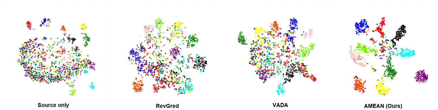
Adaptation visualization. For the BTDA transfer task mt $\rightarrow$ mm,sv,up,sy in Digit-five, we visualize the classification activations from Source-only, RevGred, VADA and AMEAN in BTDA setup. As can be seen in Fig.3 , Source-only barely captures any classification patterns. In a comparison, RevGred and VADA show better classifiable visualization patterns than Source-only’s. But their activations remain pretty messy and most of them are misaligned in their classes. It demonstrates that BTDA is a very challenging scenario for existing DA algorithms. Finally, the activations from AMEAN show clear classification margins. It illustrates the superior transferability of our AMEAN.

Ablation study. The crucial component of our AMEAN is the meta-learner for auto-designing $V_{\rm mt}$. Hence our ablation focuses on this model-driven auto-learning technique. In particular, we evaluate three adaptation manners derived from our AMEAN: adaptation without meta-learner (w/o meta learner); adaptation without meta-learner but using explicit sub-target ($\{\mathcal{T}_{j}\}^{k}_{j=1}$) to guide the transfer in BTDA (explicit sub-targets); adaptation with meta-learner (w meta-learner, AMEAN). As illustrated in Fig.4 , explicit sub-target information is not persistently helpful to BTDA. In sy-to-others, explicit sub-target information even draws back the source-to-target transfer gain. By contrast, meta-learner plays a key role to enhance the adaptation towards digit and real-world visual domains and obtain state-of-the-art in BTDA. Surprisingly, the dynamical meta-sub-targets even drive the adaptation model exceed those trained with the explicit sub-target domains.

To further investigate the meta-adaptation dynamic provided by AMEAN, we ablate the multi-target DA by following different target separation strategies: 1). explicit-sub-target (EST); 2).static deep $k$-clustering ($k$-C); 3) AMEAN. Note that, 2) ablates the auto-loss-design dynamic in $V_{\rm mt}$, as it solely uses the initial clusters to divide the mixed target and keep a static $V_{\rm mt}$ along model training. The comparison of 2) and 3) helps to unveil whether our auto-loss strategy facilitates AMEAN. As shown in Table 4 , 1) and 2) disregard label information given by a source and their $V_{\rm mt}$ still suffer from a risk of class mismatching. Our auto-loss manner adaptively changes $V_{\rm mt}$ by receiving label information from the features previously learned by Eq.1 and thus, achieve better performance in BTDA. More importantly, it also encourages a fast and more stable adaptation during the minimax optimization process (see Fig 5).

Our meta-learner $U$ is trained as deep embedding clustering (xie2016unsupervised) by receiving data and its feature-level feedbacks (the concatenation of the feature input to the discriminators and its classification result, for brevity, we mark $F(\boldsymbol{x}^{(t)})$ in our paper). It is very important to note that, distinguished from the original version solely using a DAE to initiate data embeddings, our meta-learner leverage the improved DEC guo2017improved as our implementation, where the clustering embeddings are updated by reconstruction loss as well as the clustering objective w.r.t. centroids $\{\mu_{j}\}^{k}_{j=1}$. Therefore, $U_{1}$, $U_{2}$ and $\{\mu_{j}\}^{k}_{j=1}$ are alternatively updated by

where $\alpha$ and $m$ denote the learning rate and mini-batch size for optimizing meta-learner. We set initial learning rate as $0.001$ and batch size is 256. The auto-encoder architecture implemented in our experiments has been shown in Table.5.

In our implementation, we leverage a well-known cluster assumption grandvalet2005semi to regulate the classifier $C$ learning with unlabeled target data. It can be interpreted as the minimization of the conditional entropy term with respect to the output of $C\big(F(\boldsymbol{x})\big)$

.

The objective forces the classification to be confident on the unlabeled target example, which drives the classifier’s decision boundaries away from the target unlabeled examples. It has been applied in wide range of domain adaptation researches sankaranarayanan2017generate long2016unsupervised gebru2017fine. However, while using available data to empirically estimate the expected loss, grandvalet2005semi demonstrates that such approximation provably breaks down if $C\big(F(\cdot)\big)$ does not satisfy local Lipschitz condition. Specifically, the classifier without local Lipschitz constraint can abruptly changes its prediction, which allows placement of the classifier decision boundaries close to target training examples while the empirical conditional entropy is still minimized. To prevent this issue, we follow the technique in shu2018dirt where virtual adversarial perturbation term miyato2018virtual is incorporated to regulate the classifier and feature extractor:

where $\mathbf{D}_{\rm KL}$ indicates KL divergence. $\mathbf{r}$ indicates the virtual adversarial perturbation upper bounded by a magnitude $\epsilon>0$ on source and target images ($\boldsymbol{x}^{(s)}\in\mathcal{S}$ and $\boldsymbol{x}^{(t)}\in\mathcal{T}$ ), which are obtained by maximizing the classification differences between $C\big(F(\boldsymbol{x}^{(s)})\big)$ and $C\big(F(\boldsymbol{x}^{(s)}+\mathbf{r})\big)$. This restrictions are simultaneously proposed on source and target and $\rho$ is the balance factor between them. In this way, the collaborative meta-adversarial adaptation objectives (Eq.8-10 in our paper) are reformulated as:

and

. We provide the ablation study of the entropy penalty in Table 9 .

In AMEAN, $k$ denotes the number of sub-target domains and is pre-given. Table 10 demonstrates that choosing $k$ as the number of sub-targets leads to the superior performance of AMEAN. However, whether AMEAN would achieve the better performance if $k$ is adaptively determined, remains an open and interesting question. We would like to investigate this topic in the future.

The architectures for digit recognition in Digit-five have been illustrated in Table.7 , 7 . The first backbone is based on LeNet and the second is derived from shu2018dirt for comparing their state-of-the-art models VADA and DIRT-T. The architectures for object recognition in Office-31 and Office-Home are based on AlexNet and ResNet-50, which are consistent with the previous studies long2015learning long2016deep long2016unsupervised ganin2014unsupervised .

We evenly separate the proportion of the source and target examples in each mini-batch. Concretely, we promise that a half of examples in a mini-batch are drawn from $\mathcal{S}$ and the rest belong to the mixed target domain training set $\mathcal{T}^{\rm train}$: In digit-five, we randomly drew target examples from the mixed target set $\mathcal{T}^{\rm train}$ to construct our mini-batches; In Office-31 and Office-Home, we promise the number of target examples from different meta-sub-target are the same by repeat sampling.

In the Digit-five experiment, we add a confusion loss hoffman2017simultaneous w.r.t. $\mathcal{S}$ to train the backbone-2. It stabilizes the alternating adaptation since the mixed target in Digit-five is more diverse than the other benchmarks’ and the alternating learning manner is quite instable in these scenarios. The implementation can be found in our code.

The hyper-parameters are shown in Table 8 .

We elaborate how to calculate ANT and RNT in our experiment in details:

where $Acc_{\rm Source-only}$ denotes the classification accuracy about the model trained on the source labeled dataset $\mathcal{S}$ and tested on the mixed target set $\mathcal{T}^{\rm test}=\underset{j=1}{\overset{k}{\cup}}\mathcal{T}^{\rm test}_{j}$; $Acc_{\rm BTDA}$ denotes the multi-target-weighted classification accuracy of the evaluated DA model under BTDA setup:

where $Acc_{\rm BTDA}^{(j)}$ denotes the DA model classification accuracy on the $j^{th}$ sub-target domain test set $\mathcal{T}_{j}^{\rm test}$ when the evaluated DA models (e.g., JAN, DAN, AMEAN, etc) is trained with the source labeled set $\mathcal{S}$ and the mixed target unlabeled set $\mathcal{T}^{\rm train}=\underset{j=1}{\overset{k}{\cup}}\mathcal{T}^{\rm train}_{j}$ (BTDA setup). $\{\alpha_{j}\}^{k}_{j=1}$ denotes the proportion of the multi-target mixture. It is derived from the domain-set proportion in benchmarks, which are valued by $\{0.236,0.236,0.236,0.236,0.056\}$, $\{0.686,0.121,0.193\}$ and $\{0.155,0.280,0.285,0.280\}$ in Digit-five, Office-31 and Office-Home. When we draw the subset of domains to construct the mixed target, $\{\alpha_{j}\}^{k}_{j=1}$ is obtained by normalizing these corresponding benchmark-specific domain-set proportion ²² 2 The numbers are based on the hidden sub-target test set proportions in a mixed target .

In reality, we can obtain $Acc_{\rm BTDA}$ by directly evaluating the DA models on the mixed test set $\mathcal{T}_{j}^{\rm test}$, which leads to the same results in (18).

Based on (18), we also define the RNT metric

where $Acc_{j}$ denotes the $j^{th}$-target test classification accuracy with respect to a single-target DA classifier trained on the source labeled set $\mathcal{S}$ and the $j^{th}$ sub-target unlabeled set $\mathcal{T}^{\rm train}_{j}$. Note that,

• •

  $Acc_{j}$ is derived from a DA model trained with datasets $\mathcal{S}$ and $\mathcal{T}^{\rm train}_{j}$. It means that $Acc_{i}$, $Acc_{j}$ ($i\neq j$) are derived from different DA models, which employ the same DA algorithms yet are trained on $\mathcal{T}_{i}^{\rm train}$, $\mathcal{T}_{j}^{\rm train}$ and tested on $\mathcal{T}_{i}^{\rm test}$, $\mathcal{T}_{j}^{\rm test}$, respectively.

• •

  $Acc^{(j)}_{\rm BTDA}$ is derived from a DA model trained with $\mathcal{S}$ and $\mathcal{T}^{\rm train}=\underset{j=1}{\overset{k}{\cup}}\mathcal{T}^{\rm train}_{j}$. Hence $Acc^{(i)}_{\rm BTDA}$, $Acc^{(j)}_{\rm BTDA}$ ($i\neq j$) are derived from the same DA model, which employ the same DA algorithms and is trained on ($\mathcal{S}\cup\mathcal{T}^{\rm train}$) and then, tested on $\mathcal{T}_{i}^{\rm test}$ and $\mathcal{T}_{j}^{\rm test}$ to induce $Acc^{(i)}_{\rm BTDA}$, $Acc^{(j)}_{\rm BTDA}$.

.

References

- (1) M. Andrychowicz, M. Denil, S. Gomez, M. W. Hoffman, D. Pfau, T. Schaul, B. Shillingford, and N. De Freitas. Learning to learn by gradient descent by gradient descent. In Advances in Neural Information Processing Systems, pages 3981–3989, 2016.
- (2) Anonymous. Unsupervised multi-target domain adaptation: An information theoretic approach. In Submitted to International Conference on Learning Representations, 2019. under review.
- (3) J. C. Balloch, V. Agrawal, I. Essa, and S. Chernova. Unbiasing semantic segmentation for robot perception using synthetic data feature transfer. arXiv preprint arXiv:1809.03676, 2018.
- (4) S. Ben-David, J. Blitzer, K. Crammer, A. Kulesza, F. Pereira, and J. W. Vaughan. A theory of learning from different domains. Machine learning, 79(1):151–175, 2010.
- (5) K. Bousmalis, A. Irpan, P. Wohlhart, Y. Bai, M. Kelcey, M. Kalakrishnan, L. Downs, J. Ibarz, P. Pastor, K. Konolige, et al. Using simulation and domain adaptation to improve efficiency of deep robotic grasping. In 2018 IEEE International Conference on Robotics and Automation (ICRA), pages 4243–4250. IEEE, 2018.
- (6) K. Bousmalis, N. Silberman, D. Dohan, D. Erhan, and D. Krishnan. Unsupervised pixel-level domain adaptation with generative adversarial networks. arXiv preprint arXiv:1612.05424, 2016.
- (7) Y. Chen, W. Li, C. Sakaridis, D. Dai, and L. Van Gool. Domain adaptive faster r-cnn for object detection in the wild. 2018.
- (8) C. Finn, P. Abbeel, and S. Levine. Model-agnostic meta-learning for fast adaptation of deep networks. 2017.
- (9) Y. Ganin and V. Lempitsky. Unsupervised domain adaptation by backpropagation. arXiv preprint arXiv:1409.7495, 2014.
- (10) Y. Ganin, E. Ustinova, H. Ajakan, P. Germain, H. Larochelle, F. Laviolette, M. Marchand, and V. Lempitsky. Domain-Adversarial Training of Neural Networks. 2017.
- (11) T. Gebru, J. Hoffman, and L. Fei-Fei. Fine-grained recognition in the wild: A multi-task domain adaptation approach. arXiv preprint arXiv:1709.02476, 2017.
- (12) M. Ghifary, W. B. Kleijn, M. Zhang, D. Balduzzi, and W. Li. Deep reconstruction-classification networks for unsupervised domain adaptation. In European Conference on Computer Vision, pages 597–613. Springer, 2016.
- (13) R. Gilad-Bachrach, N. Dowlin, K. Laine, K. Lauter, M. Naehrig, and J. Wernsing. Cryptonets: Applying neural networks to encrypted data with high throughput and accuracy. In International Conference on Machine Learning, pages 201–210, 2016.
- (14) I. J. Goodfellow, J. Pouget-Abadie, M. Mirza, B. Xu, D. Warde-Farley, S. Ozair, A. Courville, and Y. Bengio. Generative adversarial nets. In International Conference on Neural Information Processing Systems, pages 2672–2680, 2014.
- (15) R. Gopalan, R. Li, and R. Chellappa. Domain adaptation for object recognition: An unsupervised approach. In Computer Vision (ICCV), 2011 IEEE International Conference on, pages 999–1006. IEEE, 2011.
- (16) Y. Grandvalet and Y. Bengio. Semi-supervised learning by entropy minimization. In Advances in neural information processing systems, pages 529–536, 2005.
- (17) A. Gretton, A. J. Smola, J. Huang, M. Schmittfull, K. M. Borgwardt, and B. Schölkopf. Covariate shift by kernel mean matching. 2009.
- (18) X. Guo, L. Gao, X. Liu, and J. Yin. Improved deep embedded clustering with local structure preservation. In International Joint Conference on Artificial Intelligence (IJCAI-17), pages 1753–1759, 2017.
- (19) K. He, X. Zhang, S. Ren, and J. Sun. Deep residual learning for image recognition. 2015.
- (20) J. Hoffman, E. Tzeng, T. Darrell, and K. Saenko. Simultaneous deep transfer across domains and tasks. In Domain Adaptation in Computer Vision Applications, pages 173–187. Springer, 2017.
- (21) J. Hoffman, D. Wang, F. Yu, and T. Darrell. Fcns in the wild: Pixel-level adversarial and constraint-based adaptation. arXiv preprint arXiv:1612.02649, 2016.
- (22) A. Krizhevsky, I. Sutskever, and G. E. Hinton. Imagenet classification with deep convolutional neural networks. In Advances in neural information processing systems, pages 1097–1105, 2012.
- (23) Y. LeCun, L. Bottou, Y. Bengio, and P. Haffner. Gradient-based learning applied to document recognition. Proceedings of the IEEE, 86(11):2278–2324, 1998.
- (24) M.-Y. Liu and O. Tuzel. Coupled generative adversarial networks. In Advances in neural information processing systems, pages 469–477, 2016.
- (25) M. Long, Y. Cao, J. Wang, and M. Jordan. Learning transferable features with deep adaptation networks. In International Conference on Machine Learning, pages 97–105, 2015.
- (26) M. Long, H. Zhu, J. Wang, and M. I. Jordan. Deep transfer learning with joint adaptation networks. arXiv preprint arXiv:1605.06636, 2016.
- (27) M. Long, H. Zhu, J. Wang, and M. I. Jordan. Unsupervised domain adaptation with residual transfer networks. In Advances in Neural Information Processing Systems, pages 136–144, 2016.
- (28) M. Long, H. Zhu, J. Wang, and M. I. Jordan. Deep transfer learning with joint adaptation networks. 2017.
- (29) M. Mancini, L. Porzi, S. R. Bulò, B. Caputo, and E. Ricci. Boosting domain adaptation by discovering latent domains. arXiv preprint arXiv:1805.01386, 2018.
- (30) Y. Mansour, M. Mohri, and A. Rostamizadeh. Domain adaptation with multiple sources. In Advances in neural information processing systems, pages 1041–1048, 2009.
- (31) T. Miyato, S.-i. Maeda, S. Ishii, and M. Koyama. Virtual adversarial training: a regularization method for supervised and semi-supervised learning. IEEE transactions on pattern analysis and machine intelligence, 2018.
- (32) Y. Netzer, T. Wang, A. Coates, A. Bissacco, B. Wu, and A. Y. Ng. Reading digits in natural images with unsupervised feature learning. Nips Workshop on Deep Learning and Unsupervised Feature Learning, 2011.
- (33) S. J. Pan and Q. Yang. A survey on transfer learning. IEEE Transactions on knowledge and data engineering, 22(10):1345–1359, 2010.
- (34) A. A. Rusu, M. Vecerik, T. Rothörl, N. Heess, R. Pascanu, and R. Hadsell. Sim-to-real robot learning from pixels with progressive nets. arXiv preprint arXiv:1610.04286, 2016.
- (35) K. Saenko, B. Kulis, M. Fritz, and T. Darrell. Adapting visual category models to new domains. Computer Vision–ECCV 2010, pages 213–226, 2010.
- (36) K. Saito, Y. Ushiku, and T. Harada. Asymmetric tri-training for unsupervised domain adaptation. arXiv preprint arXiv:1702.08400, 2017.
- (37) S. Sankaranarayanan, Y. Balaji, C. D. Castillo, and R. Chellappa. Generate to adapt: Aligning domains using generative adversarial networks. ArXiv e-prints, abs/1704.01705, 2017.
- (38) R. Shu, H. H. Bui, H. Narui, and S. Ermon. A dirt-t approach to unsupervised domain adaptation. arXiv preprint arXiv:1802.08735, 2018.
- (39) E. Tzeng, J. Hoffman, K. Saenko, and T. Darrell. Adversarial discriminative domain adaptation. arXiv preprint arXiv:1702.05464, 2017.
- (40) H. Venkateswara, J. Eusebio, S. Chakraborty, and S. Panchanathan. Deep hashing network for unsupervised domain adaptation. In Proc. CVPR, pages 5018–5027, 2017.
- (41) Y. X. Wang, R. Girshick, M. Hebert, and B. Hariharan. Low-shot learning from imaginary data. 2018.
- (42) J. Xie, R. Girshick, and A. Farhadi. Unsupervised deep embedding for clustering analysis. In International conference on machine learning, pages 478–487, 2016.
- (43) H. Xu, H. Zhang, Z. Hu, X. Liang, R. Salakhutdinov, and E. Xing. Autoloss: Learning discrete schedules for alternate optimization. 2018.
- (44) R. Xu, Z. Chen, W. Zuo, J. Yan, and L. Lin. Deep cocktail network: Multi-source unsupervised domain adaptation with category shift. In Proceedings of the IEEE Conference on Computer Vision and Pattern Recognition, pages 3964–3973, 2018.
- (45) J. Yang, R. Yan, and A. G. Hauptmann. Cross-domain video concept detection using adaptive svms. In Proceedings of the 15th ACM international conference on Multimedia, pages 188–197. ACM, 2007.
- (46) L. Yang, X. Liang, T. Wang, and E. Xing. Real-to-virtual domain unification for end-to-end autonomous driving. 2018.
- (47) Y. You, X. Pan, Z. Wang, and C. Lu. Virtual to real reinforcement learning for autonomous driving. 2017.
- (48) H. Yu, M. Hu, and S. Chen. Multi-target unsupervised domain adaptation without exactly shared categories. 2018.
- (49) W. Zellinger, T. Grubinger, E. Lughofer, T. Natschläger, and S. Saminger-Platz. Central moment discrepancy (cmd) for domain-invariant representation learning. arXiv preprint arXiv:1702.08811, 2017.
- (50) H. Zhao, S. Zhang, G. Wu, J. ao P. Costeira, J. M. F. Moura, and G. J. Gordon. Multiple source domain adaptation with adversarial learning, 2018.
- (51) B. Zoph and Q. V. Le. Neural architecture search with reinforcement learning. arXiv preprint arXiv:1611.01578, 2016.