跳到论文正文
W Papers独立论文阅读器 arXiv:1907.03215 论文正文 计算阅读时间 · 0%
引用这篇论文根据当前论文元数据生成,正式投稿前建议核对。


License: arXiv.org perpetual non-exclusive license
arXiv:1907.03215v7 [cs.LG] 19 Nov 2020

Stochastic Gradient and Langevin Processes

Xiang Cheng Correspondence to: x.cheng@berkeley.edu Affiliation: Department of Electrical Engineering and Computer Science, University of California, Berkeley    Dong Yin Affiliation: Department of Electrical Engineering and Computer Science, University of California, Berkeley    Peter Bartlett Affiliation: Department of Electrical Engineering and Computer Science, University of California, Berkeley    Michael Jordan Affiliation: Department of Electrical Engineering and Computer Science, University of California, Berkeley
Abstract

We prove quantitative convergence rates at which discrete Langevin-like processes converge to the invariant distribution of a related stochastic differential equation. We study the setup where the additive noise can be non-Gaussian and state-dependent and the potential function can be non-convex. We show that the key properties of these processes depend on the potential function and the second moment of the additive noise. We apply our theoretical findings to studying the convergence of Stochastic Gradient Descent (SGD) for non-convex problems and corroborate them with experiments using SGD to train deep neural networks on the CIFAR-10 dataset.

Keywords:
Machine Learning, ICML

1 Introduction

Stochastic Gradient Descent (SGD) is one of the workhorses of modern machine learning. In many nonconvex optimization problems, such as training deep neural networks, SGD is able to produce solutions with good generalization error; indeed, there is evidence that the generalization error of an SGD solution can be significantly better than that of Gradient Descent (GD) (Keskar et al. 2016; Jastrzębski et al. 2017; He et al. 2019). This suggests that, to understand the behavior of SGD, it is not enough to consider the limiting cases such as small step size or large batch size where it degenerates to GD. In this paper, we take an alternate view of SGD as a sampling algorithm, and aim to understand its convergence to an appropriate stationary distribution.

There has been rapid recent progress in understanding the finite-time behavior of MCMC methods, by comparing them to stochastic differential equations (SDEs), such as the Langevin diffusion. It is natural in this context to think of SGD as a discrete-time approximation of an SDE. There are, however, two significant barriers to extending previous analyses to the case of SGD. First, these analysis are often restricted to isotropic Gaussian noise, whereas the noise in SGD can be far from Gaussian. Second, the noise depends significantly on the current state (the optimization variable). For instance, if the objective is an average over training data with a nonnegative loss, as the objective approaches zero the variance of minibatch SGD goes to zero. Any attempt to cast SGD as an SDE must be able to handle this kind of noise.

This motivates the study of Langevin MCMC-like methods that have a state-dependent noise term:

w(k+1)​δ=wk​δ−δ∇U(wk​δ)+δξ(wk​δ,ηk),\displaystyle w_{(k+1)\delta}=w_{k\delta}-\delta\nabla U(w_{k\delta})+\sqrt{\delta}\xi(w_{k\delta},\eta_{k}), (1)

where wt∈ℝdw_{t}\in\mathbb{R}^{d} is the state variable at time tt, δ\delta is the step size, U:ℝd→ℝU:\mathbb{R}^{d}\to\mathbb{R} is a (possibly nonconvex) potential, ξ:ℝd×Ω→ℝd\xi:\mathbb{R}^{d}\times\Omega\to\mathbb{R}^{d} is the noise function, and ηk\eta_{k} are sampled i.i.d. according to some distribution over Ω\Omega (for example, in minibatch SGD, Ω\Omega is the set of subsets of indices in the training sample).

Throughout this paper, we assume that 𝔼η​[ξ⁡(x,η)]=0\mathbb{E}_{\eta}\left[\xi(x,\eta)\right]=0 for all xx. We define a matrix-valued function M⁡(⋅):ℝd→ℝd×dM(\cdot):\mathbb{R}^{d}\to\mathbb{R}^{d\times d} to be the square root of the covariance matrix of ξ\xi; i.e., for all xx, M⁡(x):=𝔼η​[ξ⁡(x,η)​ξ​(x,η)T]M(x):=\sqrt{\mathbb{E}_{\eta}\left[\xi(x,\eta)\xi(x,\eta)^{T}\right]}, where for a positive semidefinite matrix GG, A=GA=\sqrt{G} is the unique positive semidefinite matrix such that A2=GA^{2}=G.

In studying the generalization behavior of SGD, earlier work (Jastrzębski et al. 2017; He et al. 2019) propose that (1) be approximated by the stochastic process y(k+1)​δ=yk​δ−δ∇U(yk​δ)+δM(yk​δ)θky_{(k+1)\delta}=y_{k\delta}-\delta\nabla U(y_{k\delta})+\sqrt{\delta}M(y_{k\delta})\theta_{k} where θk∼𝒩⁡(0,I)\theta_{k}\sim\mathcal{N}(0,I), or, equivalently:

d​yt=−∇U​(yk​δ)​d​t+M⁡(yk​δ)​d​Bt\displaystyle dy_{t}=-\nabla U(y_{k\delta})dt+M(y_{k\delta})dB_{t} (2)
for ​t∈[k​δ,(k+1)​δ],\displaystyle\quad\text{for }t\in[k\delta,(k+1)\delta],

with BtB_{t} denoting standard Brownian motion (Karatzas & Shreve 1998). Specifically, the non-Gaussian noise ξ⁡(⋅,η)\xi(\cdot,\eta) is approximated by a Gaussian variable M⁡(⋅)​θM(\cdot)\theta with the same covariance, via an assumption that the minibatch size is large and an appeal to the central limit theorem.

The process in (2) can be seen as the Euler-Murayama discretization of the following SDE:

d​xt=−∇U​(xt)​d​t+M⁡(xt)​d​Bt.\displaystyle dx_{t}=-\nabla U(x_{t})dt+M(x_{t})dB_{t}. (3)

We let p∗p^{*} denote the invariant distribution of (3).

We prove quantitative bounds on the discretization error between (2), (1) and (3), as well as convergence rates of (2) and (1) to p∗p^{*}. Our bounds are in Wasserstein-1 distance (denoted by W1​(⋅,⋅)W_{1}(\cdot,\cdot) in the following). We present the full theorem statements in Section 5, and summarize our contributions below:

  1. 1.

    In Theorem 1, we bound the discretization error between (2) and (3). Informally, Theorem 1 states:

    1.If x0=y0, then for all k, W1​(xk​δ,yk​δ)=O⁡(δ) ;\displaystyle 1.\ \textit{If $x_{0}=y_{0}$, then for all $k$, $W_{1}(x_{k\delta},y_{k\delta})=O(\sqrt{\delta})$ };
    2.For n≥O~​(1δ), W1​(p∗,𝖫𝖺𝗐⁡(yn​δ))=O⁡(δ),\displaystyle 2.\ \textit{For $n\geq\tilde{O}{\left(\frac{1}{\delta}\right)}$, $W_{1}(p^{*},\mathsf{Law}(y_{n\delta}))=O(\sqrt{\delta})$},

    where 𝖫𝖺𝗐⁡(⋅)\mathsf{Law}(\cdot) denotes the distribution of a random vector. This is a crucial intermediate result that allows us to prove the convergence of (1) to (3). We highlight that the variable diffusion matrix: 1) leads to a very large discretization error, due to the scaling factor of δ\sqrt{\delta} in the M⁡(yk​δ)​θkM(y_{k\delta})\theta_{k} noise term, and 2) makes the stochastic process non-contractive (this is further compounded by the non-convex drift). Our convergence proof relies on a carefully constructed Lyapunov function together with a specific coupling. Remarkably, the ϵ\epsilon dependence in our iteration complexity is the same as that in Langevin MCMC with constant isotropic diffusion (Durmus & Moulines 2016).

  2. 2.

    In Theorem 2, we bound the discretization error between (1) and (3). Informally, Theorem 2 states:

    1.If x0=w0, then for all k, W1​(xk​δ,wk​δ)=O⁡(δ1/8) ;\displaystyle 1.\ \textit{If $x_{0}=w_{0}$, then for all $k$, $W_{1}(x_{k\delta},w_{k\delta})=O(\delta^{1/8})$ };
    2.For n≥O~​(1δ), W1​(p∗,𝖫𝖺𝗐⁡(wn​δ))=O⁡(δ1/8).\displaystyle 2.\ \textit{For $n\geq\tilde{O}{\left(\frac{1}{\delta}\right)}$, $W_{1}(p^{*},\mathsf{Law}(w_{n\delta}))=O(\delta^{1/8})$}.

    Notably, the noise in each step of (1) may be far from Gaussian, but for sufficiently small step size, (1) is nonetheless able to approximate (3). This is a weaker condition than earlier work, which must assume that the batch size is sufficiently large so that CLT ensures that the per-step noise is approximately Gaussian.

  3. 3.

    Based on Theorem 2, we predict that for sufficiently small δ\delta, two different processes of the form (1) will have similar distributions if their noise terms ξ\xi have the same covariance matrix, as that leads to the same limiting SDE (3). In Section 6, we evaluate this claim empirically: we design a family of SGD-like algorithms and evaluate their test error at convergence. We observe that the noise covariance alone is a very strong predictor for the test error, regardless of higher moments of the noise. This corroborates our theoretical prediction that the noise covariance approximately determines the distribution of the solution. This is also in line with, and extends upon, observations in earlier work that the ratio of batch size to learning rate correlates with test error (Jastrzębski et al. 2017; He et al. 2019).

2 Related Work

Previous work has drawn connections between SGD noise and generalization (Mandt et al. 2016; Jastrzębski et al. 2017; He et al. 2019; Hoffer et al. 2017; Keskar et al. 2016). Notably, Mandt et al. 2016; He et al. 2019; Jastrzębski et al. 2017 analyze favorable properties of SGD noise by arguing that in the neighborhood of a local minimum, (2) is roughly the discretization of an Ornstein-Uhlenbeck (OU) process, and so the distribution of yk​δy_{k\delta} approximates is approximately Gaussian. However, empirical results (Keskar et al. 2016; Hoffer et al. 2017) suggest that SGD generalizes better by finding better local minima, which may require us to look beyond the “OU near local minimum” assumption to understand the global distributional properties of SGD. Indeed, Hoffer et al. 2017 suggest that SGD performs a random walk on a random loss landscape, Kleinberg et al. 2018 propose that SGD noise helps smoooth out “sharp minima.” Jastrzębski et al. 2017 further note the similarity between (1) and an Euler-Murayama approximation of (3). Chaudhari & Soatto 2018 also made connections between SGD and SDE. Our work tries to make these connections rigorous, by quantifying the error between (3), (2) and (1), without any assumptions about (3) being close to an OU process or being close to a local minimum.

Our work builds on a long line of work establishing the convergence rate of Langevin MCMC in different settings (Dalalyan 2017; Durmus & Moulines 2016; Ma et al. 2018; Gorham et al. 2016; Cheng et al. 2018; Erdogdu et al. 2018; Li et al. 2019). We will discuss our rates in relation to some of this work in detail following our presentation of Theorem 1. We note here that some of the techniques used in this paper were first used by Eberle 2011; Gorham et al. 2016, who analyzed the convergence of (3) to p∗p^{*} without log-concavity assumptions. Erdogdu et al. 2018 studied processes of the form (2) as an approximation to (3) under a distant-dissipativity assumption, which is similar to the assumptions made in this paper. For the sequence (2), they prove an O⁡(1/ϵ2)O(1/\epsilon^{2}) iteration complexity to achieve ϵ\epsilon integration error for any pseudo-Lipschitz loss ff with polynomial growth derivatives up to fourth order. In comparison, we prove W1W_{1} convergence between 𝖫𝖺𝗐⁡(yk​δ)\mathsf{Law}(y_{k\delta}) and p∗p^{*}, which is equivalent to sup‖∇f‖∞≤1|𝔼⁡[f⁡(yk​δ)]−𝔼y∼p∗​[f⁡(y)]|\sup_{{\left\|\nabla f\right\|}_{\infty}\leq 1}{\left|\mathbb{E}\left[{f(y_{k\delta})}\right]-\mathbb{E}_{y\sim p^{*}}\left[f(y)\right]\right|}, also with rate O~​(1/ϵ2)\tilde{O}(1/\epsilon^{2}). By smoothing the W1W_{1} test function, we believe that the results by Erdogdu et al. 2018 can imply a qualitatively similar result to Theorem 1, but with a worse dimension and ϵ\epsilon dependence.

In concurrent work by Li et al. 2019, the authors study a process based on a stochastic Runge-Kutta discretization scheme of (3). They prove an O~​(dϵ−2/3)\tilde{O}{\left(\frac{d}{\epsilon^{-2/3}}\right)} iteration complexity to achieve ϵ\epsilon error in W2W_{2} for an algorithm based on Runge-Kutta discretization of (3). They make a strong assumption of uniform dissipativity (essentially assuming that the process (3) is uniformly contractive), which is much stronger than the assumptions in this paper, and may be violated in the settings of interest considered in this paper.

There has been a number of work (Chen et al. 2016; Li et al. 2018; Anastasiou et al. 2019) which establish CLT results for SGD with very small step size (rescaled to have constant variance). These work generally focus on the setting of "OU process near a local minimum", in which the diffusion matrix is constant.

Finally, a number of authors have studied the setting of heavy-tailed gradient noise in neural network training. (Zhang et al. 2019) showed that in some cases, the heavy-tailed noise can be detrimental to training, and a clipped version of SGD performs much better. (Simsekli et al. 2019) argue that when the SGD noise is heavy-tailed, it should not be modelled as a Gaussian random variable, but instead as an α\alpha-stable random variable, and propose a Generalized Central Limit Theorem to analyze the convergence in distribution. Our paper does not handle the setting of heavy-tailed noise; our theorems require that the norm of the noise term uniformly bounded, which will be satisfied, for example, if gradients are explicitly clipped at a threshold, or if the optimization objective has Lipschitz gradients and the SGD iterates stay within a bounded region.

3 Motivating Example

It is generally difficult to write down the invariant distribution of (3). In this section, we consider a very simple one-dimensional setting which does admit an explicit expression for p∗p^{*}, and serves to illustrate some remarkable properties of anisotropic diffusion matrices.

Let us define D​(x):=M2​(x)D(x):=M^{2}(x). Our analysis will be based on the Fokker-Planck equation, which states that p∗p^{*} is the invariant distribution of (3) if

0=div(p∗(x)∇U(x))+div(p∗(x)Γ(x)+D(x)∇p∗(x)),\displaystyle 0=\textbf{div}(p^{*}(x)\nabla U(x))+\textbf{div}{\left(p^{*}(x)\Gamma(x)+D(x)\nabla p^{*}(x)\right)}, (4)

where Γ⁡(x)\Gamma(x) is a vector whose it​hi^{th} coordinate equals ∑j=1d∂∂xj​[D⁡(x)]i,j\sum_{j=1}^{d}\frac{\partial}{\partial x_{j}}{\left[D(x)\right]}_{i,j}. In the one-dimensional setting, we can explicitly write down the density of p∗​(x)p^{*}(x). Note that in this case, Γ​(x)=∇D​(x)\Gamma(x)=\nabla D(x). Let V⁡(x):=∫0x(∇U​(x)D⁡(x)+∇D​(X)D⁡(x))​𝑑x=∫0x(∇U​(x)D⁡(x))​𝑑x+log⁡D⁡(x)−log⁡D⁡(0)V(x):=\int_{0}^{x}{\left(\frac{\nabla U(x)}{D(x)}+\frac{\nabla D(X)}{D(x)}\right)}dx=\int_{0}^{x}{\left(\frac{\nabla U(x)}{D(x)}\right)}dx+\log D(x)-\log D(0). We can verify that p∗​(x)∝e−V⁡(x)p^{*}(x)\propto e^{-V(x)} satisfies (4).

For a concrete example, let the potential U⁡(x)U(x) and the diffusion function M⁡(x)M(x) be defined as

U⁡(x):={12​x2,for ​x∈[−1,4]12​(x+2)2−1,for ​x≤−112​(x−8)2−16,for ​x≥4\displaystyle U(x):=\left\{\begin{array}[]{ll}\frac{1}{2}x^{2},&\text{for }x\in[-1,4]\\ \frac{1}{2}(x+2)^{2}-1,&\text{for }x\leq-1\\ \frac{1}{2}(x-8)^{2}-16,&\text{for }x\geq 4\end{array}\right.
M⁡(x)={12​(x+2),for ​x∈[−2,8]1,for ​x≤−26,for ​x≥8.\displaystyle M(x)=\left\{\begin{array}[]{ll}\frac{1}{2}(x+2),&\text{for }x\in[-2,8]\\ 1,&\text{for }x\leq-2\\ 6,&\text{for }x\geq 8\end{array}\right..
Refer to caption
(a) U⁡(x)U(x)

Refer to caption
(b) M⁡(x)M(x)

Refer to caption
(c) V⁡(x)V(x)

Refer to caption
(d) Samples
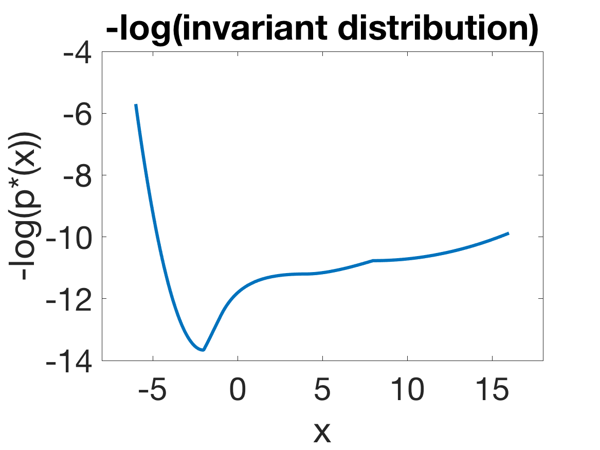
Figure 1: One-dimensional example exhibiting the importance of state-dependent noise: A simple construction showing how M⁡(x)M(x) can affect the shape of the invariant distribution. While U⁡(x)U(x) has two local minima, V⁡(x)V(x) only has the smaller minimum at x=−2x=-2. Figure 1(d) represents samples obtained from simulating using the process (2). We can see that most of the samples concentrate around x=−2x=-2.

We plot U⁡(x)U(x) in Figure 1(a). Note that U⁡(x)U(x) has two local minima: a shallow minimum at x=−2x=-2 and a deeper minimum at x=8x=8. A plot of M⁡(x)M(x) can be found in Figure 1(b). M⁡(x)M(x) is constructed to have increasing magnitude at larger values of xx. This has the effect of biasing the invariant distribution towards smaller values of xx.

We plot V⁡(x)V(x) in Figure 1(c). Remarkably, V⁡(x)V(x) has only one local minimum at x=−2x=-2. The larger minimum of U⁡(x)U(x) at x=8x=8 has been smoothed over by the effect of the large diffusion M⁡(x)M(x). This is very different from when the noise is homogeneous (e.g., M⁡(x)=IM(x)=I), in which case p∗​(x)∝e−U⁡(x)p^{*}(x)\propto e^{-U(x)}. We also simulate (3) (using (2)) for the given U⁡(x)U(x) and M⁡(x)M(x) for 1000 samples (each simulated for 1000 steps), and plot the histogram in Figure 1(d).

4 Assumptions and Definitions

In this section, we state the assumptions and definitions that we need for our main results in Theorem 1 and Theorem 2.

Assumption A

We assume that U⁡(x)U(x) satisfies

  1. 1.

    The function U⁡(x)U(x) is continuously-differentiable on ℝd\mathbb{R}^{d} and has Lipschitz continuous gradients; that is, there exists a positive constant L≥0L\geq 0 such that
    for all x,y∈ℝdx,y\in\mathbb{R}^{d}, ∥∇U​(x)−∇U​(y)∥2≤L​∥x−y∥2.\lVert\nabla U(x)-\nabla U(y)\rVert_{2}\leq L\lVert x-y\rVert_{2}.

  2. 2.

    UU has a stationary point at zero: ∇U​(0)=0.\nabla U(0)=0.

  3. 3.

    There exists a constant m>0,LR,Rm>0,L_{R},R such that for all ‖x−y‖2≥R{\left\|x-y\right\|}_{2}\geq R,

    ⟨∇𝑼(𝒙)−∇𝑼(𝒚),𝒙−𝒚≥m‖x−y‖22.\bm{\left\langle}\nabla U(x)-\nabla U(y),x-y\bm{}\geq m{\left\|x-y\right\|}_{2}^{2}. (5)

    and for all ‖x−y‖2≤R{\left\|x-y\right\|}_{2}\leq R, ∥∇U​(x)−∇U​(y)∥2≤LR​∥x−y∥2.\lVert\nabla U(x)-\nabla U(y)\rVert_{2}\leq L_{R}\lVert x-y\rVert_{2}.

Remark 1

This assumption, and minor variants, is common in the nonconvex sampling literature (Eberle 2011; Eberle 2016; Cheng et al. 2018; Ma et al. 2018; Erdogdu et al. 2018; Gorham et al. 2016).

Assumption B

We make the following assumptions on ξ\xi and MM:

  1. 1.

    For all xx, 𝔼⁡[ξ⁡(x,η)]=0\mathbb{E}\left[{\xi(x,\eta)}\right]=0.

  2. 2.

    For all xx, ‖ξ⁡(x,η)‖2≤β{\left\|\xi(x,\eta)\right\|}_{2}\leq\beta almost surely.

  3. 3.

    For all x,yx,y, ‖ξ⁡(x,η)−ξ⁡(y,η)‖2≤Lξ​‖x−y‖2{\left\|\xi(x,\eta)-\xi(y,\eta)\right\|}_{2}\leq L_{\xi}{\left\|x-y\right\|}_{2} almost surely.

  4. 4.

    There is a positive constant cmc_{m} such that for all xx, 2​cm​I≺M⁡(x)2c_{m}I\prec M(x).

Remark 2

We discuss these assumptions in a specific setting in Section 6.2.

For convenience we define a matrix-valued function N⁡(⋅):ℝd→ℝd×dN(\cdot):\mathbb{R}^{d}\to\mathbb{R}^{d\times d}:

N⁡(x):=M​(x)2−cm2​I.\displaystyle N(x):=\sqrt{M(x)^{2}-c_{m}^{2}I}. (6)

Under Assumption A, we can prove that N⁡(x)N(x) and M⁡(x)M(x) are bounded and Lipschitz (see Lemma 15 and 16 in Appendix D). These properties will be crucial in ensuring convergence.

Given an arbitrary sample space Ω\Omega and any two distribution p∈𝒫⁡(Ω)p\in\mathscr{P}{\left(\Omega\right)} and q∈𝒫⁡(Ω)q\in\mathscr{P}{\left(\Omega\right)}, a joint distribution ζ∈𝒫⁡(Ω×Ω)\zeta\in\mathscr{P}{\left(\Omega\times\Omega\right)} is a coupling between pp and qq if its marginals are equal to pp and qq respectively.

For a matrix, we use ‖G‖2{\left\|G\right\|}_{2} to denote the operator norm: ‖G‖2=supv∈ℝd,‖v‖2=1‖G​v‖2.{\left\|G\right\|}_{2}=\sup_{v\in\mathbb{R}^{d},\|v\|_{2}=1}{\left\|Gv\right\|}_{2}..

Finally, we define a few useful constants which will be used throughout the paper:

LN:=4​β​Lξcm,αq:=LR+LN22​cm2,\displaystyle L_{N}:=\frac{4\beta L_{\xi}}{c_{m}},\ \ \alpha_{q}:=\frac{L_{R}+L_{N}^{2}}{2c_{m}^{2}},
ℛq:=max⁡{R,16​β2​LNm⋅cm}\displaystyle{\mathcal{R}_{q}}:=\max\left\{R,{\frac{16\beta^{2}L_{N}}{m\cdot c_{m}}}\right\}
λ:=min⁡{m2,2​cm232​ℛq2}​exp⁡(−73​αq​ℛq2).\displaystyle\lambda:=\min\left\{\frac{m}{2},\frac{2c_{m}^{2}}{32{\mathcal{R}_{q}}^{2}}\right\}\exp{\left(-\frac{7}{3}\alpha_{q}{\mathcal{R}_{q}}^{2}\right)}. (7)

LNL_{N} is the smoothness parameter of the matrix N⁡(x)N(x), and we show in Lemma 16 that tr​((N⁡(x)−N⁡(y))2)≤LN2​‖x−y‖22\text{tr}{\left({\left(N(x)-N(y)\right)}^{2}\right)}\leq L_{N}^{2}{\left\|x-y\right\|}_{2}^{2}. The constants αq\alpha_{q} and ℛq{\mathcal{R}_{q}} are used to define a Lyapunov function qq in Appendix E.1. A key step in our proof uses the fact that, under the dynamics (2), qq contracts at a rate of e−λe^{-\lambda}, plus discretization error.

5 Main Results

In this section, we present our main convergence results beginning with convergence under Gaussian noise and proceeding to the non-Gaussian case.

Theorem 1

Let xtx_{t} and yty_{t} have dynamics as defined in (3) and (2) respectively, and suppose that the initial conditions satisfy 𝔼⁡[‖x0‖22]≤R2+β2/m\mathbb{E}\left[{{\left\|x_{0}\right\|}_{2}^{2}}\right]\leq R^{2}+\beta^{2}/m and 𝔼⁡[‖y0‖22]≤R2+β2/m\mathbb{E}\left[{{\left\|y_{0}\right\|}_{2}^{2}}\right]\leq R^{2}+\beta^{2}/m. Let ϵ^\hat{\epsilon} be a target accuracy satisfying ϵ^≤(16​(L+LN2)λ)⋅exp⁡(7​αq​ℛq/3)⋅ℛqαq​ℛq2+1\hat{\epsilon}\leq{\left(\frac{16{\left(L+L_{N}^{2}\right)}}{\lambda}\right)}\cdot\exp{\left(7\alpha_{q}{\mathcal{R}_{q}}/3\right)}\cdot\frac{{\mathcal{R}_{q}}}{\alpha_{q}{\mathcal{R}_{q}}^{2}+1}. Let δ\delta be a step size satisfying

δ≤min⁡{λ2​ϵ^2512​β2​(L2+LN4)​exp⁡(14​αq​ℛq23)2​λ​ϵ^(L2+LN4)​exp⁡(7​αq​ℛq23)​R2+β2/m.\displaystyle\delta\leq\min\left\{\begin{array}[]{ll}\frac{\lambda^{2}\hat{\epsilon}^{2}}{512\beta^{2}{\left(L^{2}+L_{N}^{4}\right)}\exp{\left(\frac{14\alpha_{q}{\mathcal{R}_{q}}^{2}}{3}\right)}}\\ \frac{2\lambda\hat{\epsilon}}{(L^{2}+L_{N}^{4})\exp{\left(\frac{7\alpha_{q}{\mathcal{R}_{q}}^{2}}{3}\right)}\sqrt{R^{2}+\beta^{2}/m}}\end{array}\right..

If we assume that x0=y0x_{0}=y_{0}, then there exists a coupling between xtx_{t} and yty_{t} such that for any kk,

𝔼⁡[‖xk​δ−yk​δ‖2]≤ϵ^\displaystyle\mathbb{E}\left[{{\left\|x_{k\delta}-y_{k\delta}\right\|}_{2}}\right]\leq\hat{\epsilon}

Alternatively, if we assume n≥3​αq​ℛq2δ​log⁡R2+β2/mϵ^n\geq\frac{3\alpha_{q}{\mathcal{R}_{q}}^{2}}{\delta}\log\frac{R^{2}+\beta^{2}/m}{\hat{\epsilon}}, then

W1​(p∗,pn​δy)≤2​ϵ^\displaystyle W_{1}{\left(p^{*},p^{y}_{n\delta}\right)}\leq 2\hat{\epsilon}

where pty:=𝖫𝖺𝗐⁡(yt)p^{y}_{t}:=\mathsf{Law}(y_{t}).

Remark 3

Note that m,L,Rm,L,R are from Assumption A, LNL_{N} is from (7), cm,β,Lξc_{m},\beta,L_{\xi} are from Assumption B).

Remark 4

Finding a suitable y0y_{0} can be done very quickly using gradient descent wrt U⁡(⋅)U(\cdot). The convergence rate to the ball of radius RR is very fast, due to Assumption A.3.

After some algebraic simplifications, we see that for a sufficiently small ϵ^\hat{\epsilon}, achieving W1​(pn​δy,p∗)≤ϵ^W_{1}(p^{y}_{n\delta},p^{*})\leq\hat{\epsilon} requires number of steps

n=O~​(β2ϵ^2⋅exp⁡(143⋅(LRcm2+16​β2​Lξ2cm4)CLOSECLOSE\displaystyle n=\tilde{O}\left(\frac{\beta^{2}}{\hat{\epsilon}^{2}}\cdot\exp\left(\frac{14}{3}\cdot{\left(\frac{L_{R}}{c_{m}^{2}}+\frac{16\beta^{2}L_{\xi}^{2}}{c_{m}^{4}}\right)}\right.\right.
⋅max{R2,212​β6​Lξ2m2​cm4})).\displaystyle\left.\left.\cdot\max\left\{R^{2},\frac{2^{12}\beta^{6}L_{\xi}^{2}}{m^{2}c_{m}^{4}}\right\}\right)\right).
Remark 5

The convergence rate contains a term eR2e^{R^{2}}; this term is also present in all of the work cited in the previous section under Remark 1. Given our assumptions, in particular 5, this dependence is unavoidable as it describes the time to transit between two modes of the invariant distribution. It can be verified to be tight by considering a simple double-well potential.

Remark 6

As illustrated in Section 6.2, the mm from Assumption B.3 should be thought of as a regularization term which can be set arbitrarily large. In the following discussion, we will assume that max⁡{R2,β6​Lξ2m2​cm4}\max\left\{R^{2},\frac{\beta^{6}L_{\xi}^{2}}{m^{2}c_{m}^{4}}\right\} is dominated by the R2R^{2} term.

To gain intuition about this term, let’s consider what it looks like under a sequence of increasingly weaker assumptions:

a. Strongly convex, constant noise: U⁡(x)U(x) mm-strongly convex, LL-smooth, ξ⁡(x,η)∼𝒩⁡(0,I)\xi(x,\eta)\sim\mathcal{N}(0,I) for all xx. (In reality we need to consider a truncated Gaussian so as not to violate Assumption B.2, but this is a minor issue). In this case, Lξ=0L_{\xi}=0, cm=1c_{m}=1, R=0R=0, β=O~​(d)\beta=\tilde{O}(\sqrt{d}), so k=O⁡(dϵ^2)k=O(\frac{d}{\hat{\epsilon}^{2}}). This is the same rate as obtained by Durmus & Moulines 2016. We remark that Durmus & Moulines 2016 obtain a W2W_{2} bound which is stronger than our W1W_{1} bound.

b. Non-convex, constant noise: U⁡(x)U(x) not strongly convex but satisfies Assumption A, and ξ⁡(x,η)∼𝒩⁡(0,I)\xi(x,\eta)\sim\mathcal{N}(0,I). In this case, Lξ=0L_{\xi}=0, cm=1c_{m}=1, β=O~​(d)\beta=\tilde{O}(\sqrt{d}) This is the setting studied by Cheng et al. 2018 and Ma et al. 2018. The rate we recover is k=O~​(dϵ2^⋅exp⁡(143​L​R2))k=\tilde{O}{\left(\frac{d}{\hat{\epsilon^{2}}}\cdot\exp{\left(\frac{14}{3}LR^{2}\right)}\right)}, which is in line with Cheng et al. 2018, and is the best W1W_{1} rate obtainable from Ma et al. 2018.

c. Non-convex, state-dependent noise: U⁡(x)U(x) satisfies Assumption A, and ξ\xi satisfies Assumption B. To simplify matters, suppose the problem is rescaled so that cm=1c_{m}=1. Then the main additional term compared to setting b. above is exp⁡(64​β2​Lξ2​R2cm4)\exp{\left(\frac{64\beta^{2}L_{\xi}^{2}R^{2}}{c_{m}^{4}}\right)}. This suggests that the effect of a LξL_{\xi}-Lipschitz noise can play a similar role in hindering mixing as a LRL_{R}-Lipschitz nonconvex drift.

When the dimension is high, computing M⁡(yk)M(y_{k}) can be difficult, but if for each xx, one has access to samples whose covariance is M⁡(x)M(x), then one can approximate M⁡(yk)​θkM(y_{k})\theta_{k} via the central limit theorem by drawing a sufficiently large number of samples. The proof of Theorem 1 can be readily modified to accommodate this (see Appendix A.5).

We now turn to the non-Gaussian case.

Theorem 2

Let xtx_{t} and wtw_{t} have dynamics as defined in (3) and (1) respectively, and suppose that the initial conditions satisfy 𝔼⁡[‖x0‖22]≤R2+β2/m\mathbb{E}\left[{{\left\|x_{0}\right\|}_{2}^{2}}\right]\leq R^{2}+\beta^{2}/m and 𝔼⁡[‖w0‖22]≤R2+β2/m\mathbb{E}\left[{{\left\|w_{0}\right\|}_{2}^{2}}\right]\leq R^{2}+\beta^{2}/m. Let ϵ^\hat{\epsilon} be a target accuracy satisfying ϵ^≤(16​(L+LN2)λ)⋅exp⁡(7​αq​ℛq/3)⋅ℛqαq​ℛq2+1\hat{\epsilon}\leq{\left(\frac{16{\left(L+L_{N}^{2}\right)}}{\lambda}\right)}\cdot\exp{\left(7\alpha_{q}{\mathcal{R}_{q}}/3\right)}\cdot\frac{{\mathcal{R}_{q}}}{\alpha_{q}{\mathcal{R}_{q}}^{2}+1}. Let ϵ:=λ16​(L+LN2)​exp⁡(−7​αq​ℛq23)​ϵ^\epsilon:=\frac{\lambda}{16(L+L_{N}^{2})}\exp{\left(-\frac{7\alpha_{q}{\mathcal{R}_{q}}^{2}}{3}\right)}\hat{\epsilon}. Let T:=min⁡{116​L,β28​L2​(R2+β2/m),ϵ32​L​β,ϵ2128​β2,ϵ4​LN2214​β2​cm2}T:=\min\left\{\frac{1}{16L},\frac{\beta^{2}}{8L^{2}{\left(R^{2}+\beta^{2}/m\right)}},\frac{\epsilon}{32\sqrt{L}\beta},\frac{\epsilon^{2}}{128\beta^{2}},\frac{\epsilon^{4}L_{N}^{2}}{2^{14}\beta^{2}c_{m}^{2}}\right\} and let δ\delta be a step size satisfying

δ≤min⁡{T​ϵ2​L36​d​β2​log⁡(36​d​β2ϵ2​L),T​ϵ4​L2214​d​β4​log⁡(214​d​β4ϵ4​L2)}.\displaystyle\delta\leq\min\left\{\frac{T\epsilon^{2}L}{36d\beta^{2}\log{\left(\frac{36d\beta^{2}}{\epsilon^{2}L}\right)}},\frac{T\epsilon^{4}L^{2}}{2^{14}d\beta^{4}\log{\left(\frac{2^{14}d\beta^{4}}{\epsilon^{4}L^{2}}\right)}}\right\}.

If we assume that x0=w0x_{0}=w_{0}, then there exists a coupling between xtx_{t} and wtw_{t} such that for any kk,

𝔼⁡[‖xk​δ−wk​δ‖2]≤ϵ^.\displaystyle\mathbb{E}\left[{{\left\|x_{k\delta}-w_{k\delta}\right\|}_{2}}\right]\leq\hat{\epsilon}.

Alternatively, if we assume that n≥3​αq​ℛq2δ⋅log⁡R2+β2/mϵ^n\geq\frac{3\alpha_{q}{\mathcal{R}_{q}}^{2}}{\delta}\cdot\log\frac{R^{2}+\beta^{2}/m}{\hat{\epsilon}}, then

W1​(p∗,pn​δw)≤2​ϵ^,\displaystyle W_{1}{\left(p^{*},p^{w}_{n\delta}\right)}\leq 2\hat{\epsilon},

where ptw:=𝖫𝖺𝗐⁡(wt)p^{w}_{t}:=\mathsf{Law}(w_{t}).

Remark 7

To achieve W1​(p∗,pn​δw)≤ϵ^W_{1}(p^{*},p^{w}_{n\delta})\leq\hat{\epsilon}, the number of steps needed is of order n=O~​(1ϵ^8⋅e29​αq​ℛq2)n=\tilde{O}{\left(\frac{1}{\hat{\epsilon}^{8}}\cdot e^{29\alpha_{q}{\mathcal{R}_{q}}^{2}}\right)}. The ϵ^\hat{\epsilon} dependency is considerably worse than in Theorem 1. This is because we need to take many steps of (1) in order to approximate a single step of (2). For details, see the coupling construction in equations (27)–(31) of Appendix B.

6 Application to Stochastic Gradient Descent

In this section, we will cast SGD in the form of (1). We consider an objective of the form

U⁡(w)=1n​∑i=1nUi​(w).\displaystyle U(w)=\frac{1}{n}\sum_{i=1}^{n}U_{i}(w). (8)

We reserve the letter η\eta to denote a random minibatch from {1,…,n}\left\{1,\ldots,n\right\}, sampled with replacement, and define ζ⁡(w,η)\zeta(w,\eta) as follows:

ζ⁡(w,η):=∇U​(w)−1|η|​∑i∈η∇Ui​(w)\zeta(w,\eta):=\nabla U(w)-\frac{1}{{\left|\eta\right|}}\sum_{i\in\eta}\nabla U_{i}(w) (9)

For a sample of size one, i.e. |η|=1{\left|\eta\right|}=1, we define

H⁡(w):=𝔼⁡[ζ⁡(w,η)​ζ​(w,η)T]\displaystyle H(w):=\mathbb{E}\left[{\zeta(w,\eta)\zeta(w,\eta)^{T}}\right] (10)

as the covariance matrix of the difference between the true gradient and a single sampled gradient at ww. A standard run of SGD, with minibatch size b:=|ηk|b:={\left|\eta_{k}\right|}, then has the following form:

wk+1\displaystyle w_{k+1} =wk−δ​1b​∑i∈ηk∇Ui​(wk)\displaystyle=w_{k}-\delta\frac{1}{b}\sum_{i\in\eta_{k}}\nabla U_{i}(w_{k})
=wk−δ∇U(wk)+δ(δζ(wk,ηk)).\displaystyle=w_{k}-\delta\nabla U(w_{k})+\sqrt{\delta}{\left(\sqrt{\delta}\zeta(w_{k},\eta_{k})\right)}. (11)

We refer to an SGD algorithm with step size δ\delta and minibatch size bb a (δ,b)(\delta,b)-SGD. Notice that (11) is in the form of (1), with ξ⁡(w,η)=δ​ζ​(w,η)\xi(w,\eta)=\sqrt{\delta}\zeta(w,\eta). The covariance matrix of the noise term is

𝔼⁡[ξ⁡(w,η)​ξ​(w,η)T]=δb​H​(w).\mathbb{E}\left[{\xi(w,\eta)\xi(w,\eta)^{T}}\right]=\frac{\delta}{b}H(w). (12)

Because the magnitude of the noise covariance scales with δ\sqrt{\delta}, it follows that as δ→0\delta\to 0, (11) converges to deterministic gradient flow. However, the loss of randomness as δ→0\delta\to 0 is not desirable as it has been observed that as SGD approaches GD, through either small step size or large batch size, the generalization error goes up (Jastrzębski et al. 2017; He et al. 2019; Keskar et al. 2016; Hoffer et al. 2017); this is also consistent with our experimental observations in Section 6.3.1.

Therefore, a more meaningful way to take the limit of SGD is to hold the noise term constant in (11). More specifically, we define the constant-noise limit of (11) as

d​xt=−∇U​(xt)​d​t+M⁡(xt)​d​Bt,dx_{t}=-\nabla U(x_{t})dt+M(x_{t})dB_{t}, (13)

where M⁡(x):=δb​H​(x)M(x):=\sqrt{\frac{\delta}{b}H(x)}. Note that this is in the form of (3), with noise covariance M​(xt)2M(x_{t})^{2} matching that of SGD in (11). Using Theorem 2, we can bound the W1W_{1} distance between the SGD iterates wkw_{k} from (11), and the continuous-time SDE xtx_{t} from (13).

6.1 Importance of Noise Covariance

We highlight the fact that the limiting SDE of a discrete process,

wk+1=wk−s∇U(wk)+sξ(wk,ηk),w_{k+1}=w_{k}-s\nabla U(w_{k})+\sqrt{s}\xi(w_{k},\eta_{k}), (14)

depends only on the covariance matrix of ξ\xi. More specifically, as long as ξ\xi satisfies 𝔼⁡[ξ⁡(w,η)​ξ​(w,η)T]=M⁡(w)\sqrt{\mathbb{E}\left[{\xi(w,\eta)\xi(w,\eta)^{T}}\right]}=M(w), (14) will have (13) as its limiting SDE, regardless of higher moments of ξ\xi. This fact, combined with Theorem 2, means that in the limit of δ→0\delta\to 0 and k→∞k\to\infty, the distribution of wkw_{k} will be determined by the covariance of ξ\xi alone. An immediate consequence is the following: at convergence, the test performance of any Langevin MCMC-like algorithm is almost entirely determined by the covariance of its noise term.

Returning to the case of SGD algorithms, since the noise covariance is M​(x)2=δb​H​(x)M(x)^{2}=\frac{\delta}{b}H(x) (see (12)), we know that the ratio of step size δ\delta to batch size bb is an important quantity which can dictate the test error of the algorithm; this observation has been made many times in prior work (Jastrzębski et al. 2017; He et al. 2019), and our results in this paper are in line with these observations. Here, we move one step further, and provide experimental evidence to show that more fundamentally, it is the noise covariance in the constant-noise limit that controls the test error.

To verify this empirically, we propose the following algorithm called large-noise SGD.

Definition 1

An (s,σ,b1,b2)(s,\sigma,b_{1},b_{2})-large-noise SGD is an algorithm that aims to minimize (8) using the following updates:

wk+1=wk−sb1​∑i∈ηk∇Ui​(wk)\displaystyle w_{k+1}=w_{k}-\frac{s}{b_{1}}\sum_{i\in\eta_{k}}\nabla U_{i}(w_{k}) (15)
+σ​sb2​(∑i∈ηk′∇Ui​(wk)−∑i∈ηk′′∇Ui​(wk)),\displaystyle\qquad+\frac{\sigma\sqrt{s}}{b_{2}}\left(\sum_{i\in\eta_{k}^{\prime}}\nabla U_{i}(w_{k})-\sum_{i\in\eta_{k}^{\prime\prime}}\nabla U_{i}(w_{k})\right),

where ηk\eta_{k}, ηk′\eta_{k}^{\prime}, and ηk′′\eta_{k}^{\prime\prime} are minibatches of sizes b1b_{1}, b2b_{2}, and b2b_{2}, sampled uniformly at random from {1,…,n}\{1,\ldots,n\} with replacement. The three minibatches are sampled independently and are also independent of other iterations.

Intuitively, an (s,σ,b1,b2)(s,\sigma,b_{1},b_{2})-large-noise SGD should be considered as an SGD algorithm with step size ss and minibatch size b1b_{1} and an additional noise term. The noise term computes the difference of two independent and unbiased estimates of the full gradient ∇U​(wk)\nabla U(w_{k}), each using a batch of b2b_{2} data points. Using the definition of ζ\zeta in (9), we can verify that the update (15) is equivalent to

wk+1=wk−s∇U(wk)+sζ(wk,ηk)\displaystyle w_{k+1}=w_{k}-s\nabla U(w_{k})+s\zeta(w_{k},\eta_{k}) (16)
+σ​s​(ζ⁡(wk,ηk′′)−ζ⁡(wk,ηk′)),\displaystyle\qquad+\sigma\sqrt{s}(\zeta(w_{k},\eta_{k}^{\prime\prime})-\zeta(w_{k},\eta_{k}^{\prime})),

which is in the form of (1), with

ξ⁡(w,η~)=s​ζ​(w,η)+σ⁡(ζ⁡(w,η′′)−ζ⁡(w,η′)),\displaystyle\xi(w,\tilde{\eta})=\sqrt{s}\zeta(w,\eta)+\sigma{\left(\zeta(w,\eta^{\prime\prime})-\zeta(w,\eta^{\prime})\right)}, (17)

where η~=(η,η′,η′′)\tilde{\eta}=(\eta,\eta^{\prime},\eta^{\prime\prime}), and |η|=b1|\eta|=b_{1}, |η′|=|η′′|=b2|\eta^{\prime}|=|\eta^{\prime\prime}|=b_{2}. Further, the noise covariance matrix is

𝔼⁡[ξ⁡(w,η~)​ξ​(w,η~)T]=(sb1+2​σ2b2)​H​(w).\mathbb{E}\left[{\xi(w,\tilde{\eta})\xi(w,\tilde{\eta})^{T}}\right]=(\frac{s}{b_{1}}+\frac{2\sigma^{2}}{b_{2}})H(w). (18)

Therefore, if we have

sb1+2​σ2b2=δb,\frac{s}{b_{1}}+\frac{2\sigma^{2}}{b_{2}}=\frac{\delta}{b}, (19)

then an (s,σ,b1,b2)(s,\sigma,b_{1},b_{2})-large-noise SGD should have the same noise covariance as a (δ,b)(\delta,b)-SGD (but very different higher noise moments due to the injected noise), and based on our theory, the large-noise SGD should have similar test error to that of the SGD algorithm, even if the step size and batch size are different. In Section 6.3, we verify this experimentally. We stress that we are not proposing the large-noise SGD as a practical algorithm. The reason that this algorithm is interesting is that it gives us a family of (wk)k=1,2,…{\left(w_{k}\right)}_{k=1,2,\ldots} which converges to (13), and is implementable in practice. Thus this algorithm helps us uncover the importance of noise covariance (and the unimportance of higher noise moments) in Langevin MCMC-like algorithms. We also remark that Hoffer et al. 2017 proposed a different way of injecting noise, multiplying the sampled gradient with a suitably scaled Gaussian noise.

6.2 Satisfying the Assumptions

Before presenting the experimental results, we remark on a particular way that a function U⁡(w)U(w) defined in (8), along with the stochastic sequence wkw_{k} defined in (15), can satisfy the assumptions in Section 4.

Suppose first that we shift the coordinate system so that ∇U​(0)=0\nabla U(0)=0. Let us additionally assume that for each ii, Ui​(w)U_{i}(w) has the form

Ui​(w)=Ui′​(w)+V⁡(w),\displaystyle U_{i}(w)=U_{i}^{\prime}(w)+V(w),

where V⁡(w):=m​(‖x‖2−R/2)2V(w):=m{\left(\|x\|_{2}-R/2\right)}^{2} is a mm-strongly convex regularizer outside a ball of radius RR, and each Ui′​(w)U_{i}^{\prime}(w) has LRL_{R}-Lipschitz gradients. Suppose further that m≥4⋅LRm\geq 4\cdot L_{R}. These additional assumptions make sense when we are only interested in U⁡(w)U(w) over BR​(0)B_{R}(0), so V⁡(w)V(w) plays the role of a barrier function that keeps us within BR​(0)B_{R}(0). Then, it can immediately be verified that U⁡(w)U(w) satisfies Assumption A with L=m+LRL=m+L_{R}.

The noise term ξ\xi in (17) satisfies Assumption B.1 by definition, and satisfies Assumption B.3 with Lξ=(s+2​σ)​LL_{\xi}={\left(\sqrt{s}+2\sigma\right)}L. Assumption B.2 is satisfied if ζ⁡(w,η)\zeta(w,\eta) is bounded for all ww, i.e. the sampled gradient does not deviate from the true gradient by more than a constant. We will need to assume directly Assumption B.4, as it is a property of the distribution of ∇Ui​(w)\nabla U_{i}(w) for i=1,…,ni=1,\ldots,n.

Figure 2: Relationship between test accuracy and the noise covariance of SGD algorithm. In each plot, the dots with the same color correspond to SGD runs with the same batch size but different step sizes.

6.3 Experiments

Figure 3: Large-noise SGD. Small dots correspond to all the baseline SGD runs in Figure 2. Each ×\times corresponds to a baseline SGD run whose step size is specified in the legend and batch size is specified in the title. Each ⋄\diamond corresponds to a large-noise SGD run whose noise covariance is 88 times of that of the ×\times with the same color. As we can see, injecting noise improves test accuracy, and the large-noise SGD runs fall close to the linear trend.
Figure 4: Large-noise SGD. Batch size in the titles represents the batch size of ×\times runs. Each ⋄\diamond corresponds to a large-noise SGD run whose noise covariance matches that of a baseline SGD run whose step size is the same as the ×\times run with the same color and batch size is 128128. Again, large-noise SGD falls close to the linear trend.

In this section, we present experimental results that validate the importance of noise covariance in predicting the test error of Langevin MCMC-like algorithms. Our experiment code can be found at https://github.com/dongyin92/noise_covariance.

In all experiments, we use two different neural network architectures on the CIFAR-10 dataset (Krizhevsky & Hinton 2009) with the standard test-train split. The first architecture is a simple convolutional neural network, which we call CNN in the following,11 1 We provide details of this CNN architecture in Appendix G. and the other is the VGG19 network (Simonyan & Zisserman 2014). To make our experiments consistent with the setting of SGD, we do not use batch normalization or dropout, and use constant step size. In all of our experiments, we run SGD algorithm 20002000 epochs such that the algorithm converges sufficiently. Since in most of our experiments, the accuracies on the training dataset are almost 100%100\%, we use the test accuracy to measure the generalization performance.

Recall that according to (12) and (18), for both SGD and large-noise SGD, the noise covariance is a scalar multiple of H⁡(w)H(w). For simplicity, in the following, we will slightly abuse our terminology and call this scalar the noise covariance; more specifically, for (δ,b)(\delta,b)-SGD, the noise covariance is δ/b\delta/b, and for an (s,σ,b1,b2)(s,\sigma,b_{1},b_{2})-large-noise SGD, the noise covariance is sb1+2​σ2b2\frac{s}{b_{1}}+\frac{2\sigma^{2}}{b_{2}}.

6.3.1 Accuracy vs Noise Covariance

In our first experiment, we focus on the SGD algorithm, and show that there is a positive correlation between the noise covariance and the final test accuracy of the trained model. One major purpose of this experiment is to establish baselines for our experiments on large-noise SGD.

We choose constant step size δ\delta from

{0.001,0.002,0.004,0.008,0.016,0.032,0.064,0.128}\{0.001,0.002,0.004,0.008,0.016,0.032,0.064,0.128\}

and minibatch size bb from {32,64,128,256,512}\{32,64,128,256,512\}. For each (step size, batch size) pair, we plot its final test accuracy against its noise covariance in Figure 2. From the plot, we can see that higher noise covariance leads to better final test accuracy, and there is a linear trend between the test accuracy and the logarithm. We also highlight the fact that conditioned on the noise covariance, the test accuracy is not significantly correlated with either the step size or the minibatch size. In other words, similar to the observations in prior work (Jastrzębski et al. 2017; He et al. 2019), there is a strong correlation between relative variance of an SGD sequence and its test accuracy, regardless of the combination of minibatch size and step size.

6.3.2 Large-Noise SGD

In this section, we implement and examine the performance of the large-noise SGD algorithm proposed in (15). We select a subset of SGD runs with relatively small noise covariance in the experiment in the previous section (we call them baseline SGD runs), and implement large-noise SGD by injecting noise. Our goal is to see, for a particular noise covariance, whether large-noise SGD has test accuracy that is similar to SGD, in spite of significant differences in third-and-higher moments of the noise in large-noise SGD compared to standard SGD.

Our first experiment is to add noise with the same minibatch size to the (δ,b)(\delta,b) baseline SGD run such that the new noise covariance matches that of an (8​δ,b)(8\delta,b)-SGD (an SGD run with larger step size). In other words, we implement (δ,7​δ/2,b,b)(\delta,\sqrt{7\delta/2},b,b)-large-noise SGD, whose noise covariance is 88 times of that of the baseline. Our results are shown in Figure 3. Our second experiment is similar: we add noise with minibatch size 128128 to the (δ,b)(\delta,b) baseline SGD run with b∈{256,512}b\in\{256,512\} such that the new noise covariance matches that of a (δ,128)(\delta,128)-SGD (an SGD run with smaller batch size). More specifically, we implement (δ,12​(1−128b)​δ,b,128)(\delta,\sqrt{\frac{1}{2}(1-\frac{128}{b})\delta},b,128)-large-noise SGD runs. The results are shown in Figure 4. In these figures, each ×\times denotes a baseline SGD run, with step size specified in the legend and minibatch size specified by plot title. For each baseline SGD run, we have a corresponding large-noise SGD run, denoted by ⋄\diamond with the same color. As mentioned, these ⋄\diamond runs are designed to match the noise covariance of SGD with larger step size or smaller batch size. In addition to ×\times and ⋄\diamond, we also plot using a small teal marker all the other runs from Section 6.3.1. This helps highlight the linear trend between the logarithm of noise covariance and test accuracy that we observed in Section 6.3.1.

As can be seen, the (noise variance, test accuracy) values for the ⋄\diamond runs fall close to the linear trend. More specifically, a run of large-noise SGD produces similar test accuracy to vanilla SGD runs with the same noise variance. We highlight two potential implications: First, just like in Section 6.3.1, we observe that the test accuracy strongly correlates with relative variance, even for noise of the form (17), which can have rather different higher moments than ζ\zeta (standard SGD noise); Second, since the ⋄\diamond points fall close to the linear trend, we hypothesize that the constant-noise limit SDE (13) should also have similar test error. If true, then this implies that we only need to study the potential U⁡(x)U(x) and noise covariance M⁡(x)M(x) to explain the generalization properties of SGD.

7 Acknowledgements

We wish to acknowledge support by the Army Research Office (ARO) under contract W911NF-17-1-0304 under the Multidisciplinary University Research Initiative (MURI).

References

  • Anastasiou et al. (2019) Anastasiou, A., Balasubramanian, K., and Erdogdu, M. A. Normal approximation for stochastic gradient descent via non-asymptotic rates of martingale CLT. arXiv preprint arXiv:1904.02130, 2019.
  • Chatzigeorgiou (2013) Chatzigeorgiou, I. Bounds on the Lambert function and their application to the outage analysis of user cooperation. IEEE Communications Letters, 17(8):1505–1508, 2013.
  • Chaudhari & Soatto (2018) Chaudhari, P. and Soatto, S. Stochastic gradient descent performs variational inference, converges to limit cycles for deep networks. In 2018 Information Theory and Applications Workshop (ITA), pp. 1–10. IEEE, 2018.
  • Chen et al. (2016) Chen, X., Lee, J. D., Tong, X. T., and Zhang, Y. Statistical inference for model parameters in stochastic gradient descent. arXiv preprint arXiv:1610.08637, 2016.
  • Cheng et al. (2018) Cheng, X., Chatterji, N. S., Abbasi-Yadkori, Y., Bartlett, P. L., and Jordan, M. I. Sharp convergence rates for Langevin dynamics in the nonconvex setting. arXiv preprint arXiv:1805.01648, 2018.
  • Cheng et al. (2019) Cheng, X., Bartlett, P. L., and Jordan, M. I. Quantitative central limit theorems for discrete stochastic processes. arXiv preprint arXiv:1902.00832, 2019.
  • Dalalyan (2017) Dalalyan, A. S. Theoretical guarantees for approximate sampling from smooth and log-concave densities. Journal of the Royal Statistical Society: Series B (Statistical Methodology), 79(3):651–676, 2017.
  • Durmus & Moulines (2016) Durmus, A. and Moulines, E. High-dimensional Bayesian inference via the unadjusted langevin algorithm. arXiv preprint arXiv:1605.01559, 2016.
  • Eberle (2011) Eberle, A. Reflection coupling and Wasserstein contractivity without convexity. Comptes Rendus Mathematique, 349(19-20):1101–1104, 2011.
  • Eberle (2016) Eberle, A. Reflection couplings and contraction rates for diffusions. Probability theory and related fields, 166(3-4):851–886, 2016.
  • Eldan et al. (2018) Eldan, R., Mikulincer, D., and Zhai, A. The CLT in high dimensions: quantitative bounds via martingale embedding. arXiv preprint arXiv:1806.09087, 2018.
  • Erdogdu et al. (2018) Erdogdu, M. A., Mackey, L., and Shamir, O. Global non-convex optimization with discretized diffusions. In Advances in Neural Information Processing Systems, pp. 9671–9680, 2018.
  • Gorham et al. (2016) Gorham, J., Duncan, A. B., Vollmer, S. J., and Mackey, L. Measuring sample quality with diffusions. arXiv preprint arXiv:1611.06972, 2016.
  • He et al. (2019) He, F., Liu, T., and Tao, D. Control batch size and learning rate to generalize well: Theoretical and empirical evidence. In Advances in Neural Information Processing Systems, pp. 1141–1150, 2019.
  • Hoffer et al. (2017) Hoffer, E., Hubara, I., and Soudry, D. Train longer, generalize better: closing the generalization gap in large batch training of neural networks. In Advances in Neural Information Processing Systems, pp. 1731–1741, 2017.
  • Jastrzębski et al. (2017) Jastrzębski, S., Kenton, Z., Arpit, D., Ballas, N., Fischer, A., Bengio, Y., and Storkey, A. Three factors influencing minima in SGD. arXiv preprint arXiv:1711.04623, 2017.
  • Karatzas & Shreve (1998) Karatzas, I. and Shreve, S. E. Brownian motion. In Brownian Motion and Stochastic Calculus, pp. 47–127. Springer, 1998.
  • Keskar et al. (2016) Keskar, N. S., Mudigere, D., Nocedal, J., Smelyanskiy, M., and Tang, P. T. P. On large-batch training for deep learning: Generalization gap and sharp minima. arXiv preprint arXiv:1609.04836, 2016.
  • Kleinberg et al. (2018) Kleinberg, R., Li, Y., and Yuan, Y. An alternative view: When does SGD escape local minima? arXiv preprint arXiv:1802.06175, 2018.
  • Krizhevsky & Hinton (2009) Krizhevsky, A. and Hinton, G. Learning multiple layers of features from tiny images. Technical report, Citeseer, 2009.
  • Li et al. (2018) Li, T., Liu, L., Kyrillidis, A., and Caramanis, C. Statistical inference using sgd. In Thirty-Second AAAI Conference on Artificial Intelligence, 2018.
  • Li et al. (2019) Li, X., Wu, Y., and Mackey, L. Stochastic Runge-Kutta accelerates Langevin Monte Carlo and beyond. In Advances in Neural Information Processing Systems, pp. 7746–7758, 2019.
  • Ma et al. (2018) Ma, Y.-A., Chen, Y., Jin, C., Flammarion, N., and Jordan, M. I. Sampling can be faster than optimization. arXiv preprint arXiv:1811.08413, 2018.
  • Mandt et al. (2016) Mandt, S., Hoffman, M., and Blei, D. A variational analysis of stochastic gradient algorithms. In International Conference on Machine Learning, pp. 354–363, 2016.
  • Simonyan & Zisserman (2014) Simonyan, K. and Zisserman, A. Very deep convolutional networks for large-scale image recognition. arXiv preprint arXiv:1409.1556, 2014.
  • Simsekli et al. (2019) Simsekli, U., Sagun, L., and Gurbuzbalaban, M. A tail-index analysis of stochastic gradient noise in deep neural networks. arXiv preprint arXiv:1901.06053, 2019.
  • Zhang et al. (2019) Zhang, J., Karimireddy, S. P., Veit, A., Kim, S., Reddi, S. J., Kumar, S., and Sra, S. Why adam beats sgd for attention models. arXiv preprint arXiv:1912.03194, 2019.

Appendix

Appendix A Proofs for Convergence under Gaussian Noise (Theorem 1)

A.1 Proof Overview

The main proof of Theorem 1 is contained in Appendix A.4.

Here, we outline the steps of our proof:

  1. 1.

    In Appendix A.2, we construct a coupling between (3) and (2) over a single step (i.e. for t∈[k​δ,(k+1)​δ]t\in[k\delta,(k+1)\delta], for some kk and δ\delta).

  2. 2.

    Appendix A.3, we prove Lemma 1, which shows that under the coupling constructed in Step 1, a Lyapunov function f⁡(xT−yT)f(x_{T}-y_{T}) contracts exponentially with rate λ\lambda, plus a discretization error term. The function ff is defined in Appendix E, and sandwiches ‖xT−yT‖2{\left\|x_{T}-y_{T}\right\|}_{2}. In Corollary 2, we apply the results of Lemma 1 recursively over multiple steps to give a bound on f⁡(xk​δ−yk​δ)f(x_{k\delta}-y_{k\delta}) for all kk, and for sufficiently small δ\delta.

  3. 3.

    Finally, in Appendix A.4, we prove Theorem 1 by applying the results of Corollary 2, together with the fact that f⁡(z)f(z) upper bounds ‖z‖2{\left\|z\right\|}_{2} up to a constant factor.

A.2 A coupling construction

In this subsection, we will study the evolution of (3) and (2) over a small time interval. Specifically, we will study

d​xt=\displaystyle dx_{t}= −∇U​(xt)​d​t+M⁡(xt)​d​Bt\displaystyle-\nabla U(x_{t})dt+M(x_{t})dB_{t} (20)
d​yt=\displaystyle dy_{t}= −∇U​(y0)​d​t+M⁡(y0)​d​Bt\displaystyle-\nabla U(y_{0})dt+M(y_{0})dB_{t} (21)

One can verify that (20) is equivalent to (3), and (21) is equivalent to a single step of (2) (i.e. over an interval t≤δt\leq\delta).

We first give the explicit coupling between (20) and (21): ( A similar coupling in the continuous-time setting is first seen in (Gorham et al. 2016) in their proof of contraction of (3).)

Given arbirary (x0,y0)(x_{0},y_{0}), define (xt,yt)(x_{t},y_{t}) using the following coupled SDE:

xt=\displaystyle x_{t}= x0+∫0t−∇U(xs)ds+∫0tcmdVs+∫0tN(xs)dWs\displaystyle x_{0}+\int_{0}^{t}-\nabla U(x_{s})ds+\int_{0}^{t}c_{m}dV_{s}+\int_{0}^{t}N(x_{s})dW_{s} (22)
yt=\displaystyle y_{t}= y0+∫0t−∇U(y0)dt+∫0tcm(I−2γsγsT)dVs+∫0tN(y0)dWs\displaystyle y_{0}+\int_{0}^{t}-\nabla U(y_{0})dt+\int_{0}^{t}c_{m}{\left(I-2\gamma_{s}\gamma_{s}^{T}\right)}dV_{s}+\int_{0}^{t}N(y_{0})dW_{s}

Where d​VtdV_{t} and d​WtdW_{t} are two independent standard Brownian motion, and

γt:=xt−yt‖xt−y‖2⋅𝟙{∥xt−yt∥2∈[2ϵ,ℛq)}\displaystyle\gamma_{t}:=\frac{x_{t}-y_{t}}{\|x_{t}-y\|_{2}}\cdot{\mathbbm{1}\left\{\|x_{t}-y_{t}\|_{2}\in[2\epsilon,{\mathcal{R}_{q}})\right\}} (23)

By Lemma 6, we show that (20) has the same distribution as xtx_{t} in (22), and (21) has the same distribution as yty_{t} in (22). Thus, for any tt, the process (xt,yt)(x_{t},y_{t}) defined by (22) is a valid coupling for (20) and (21).

A.3 One step contraction

Lemma 1

Let ff be as defined in Lemma 18 with parameters ϵ\epsilon satisfying ϵ≤ℛqαq​ℛq2+1\epsilon\leq\frac{{\mathcal{R}_{q}}}{\alpha_{q}{\mathcal{R}_{q}}^{2}+1}. Let xtx_{t} and yty_{t} be as defined in (22). If we assume that 𝔼⁡[‖y0‖22]≤8​(R2+β2/m)\mathbb{E}\left[{{\left\|y_{0}\right\|}_{2}^{2}}\right]\leq 8{\left(R^{2}+\beta^{2}/m\right)} and T≤min⁡{ϵ2β2,ϵ6​L​R2+β2/m}T\leq\min\left\{\frac{\epsilon^{2}}{\beta^{2}},\frac{\epsilon}{6L\sqrt{R^{2}+\beta^{2}/m}}\right\}, then

𝔼⁡[f⁡(xT−yT)]≤e−λ​T​𝔼​[f⁡(x0−y0)]+3​T​(L+LN2)​ϵ\displaystyle\mathbb{E}\left[{f(x_{T}-y_{T})}\right]\leq e^{-\lambda T}\mathbb{E}\left[{f(x_{0}-y_{0})}\right]+3T(L+L_{N}^{2})\epsilon
Remark 8

For ease of reference: m,L,LR,Rm,L,L_{R},R are from Assumption A, cm,βc_{m},\beta are from Assumption B, αq,ℛq,LN,λ\alpha_{q},{\mathcal{R}_{q}},L_{N},\lambda are defined in (7).


For notational convenience, for the rest of this proof, let us define zt:=xt−ytz_{t}:=x_{t}-y_{t} and ∇t:=∇U​(xt)−∇U​(yt)\nabla_{t}:=\nabla U(x_{t})-\nabla U(y_{t}), Δt:=∇U​(y0)−∇U​(yt)\Delta_{t}:=\nabla U(y_{0})-\nabla U(y_{t}) Nt:=N⁡(xt)−N⁡(yt)N_{t}:=N(x_{t})-N(y_{t}).

It follows from (22) that

d​zt=−∇td​t+Δt​d​t+2​cm​γt​γtT​d​Vt+(Nt+N⁡(yt)−N⁡(y0))​d​Wt\displaystyle dz_{t}=-\nabla_{t}dt+\Delta_{t}dt+2c_{m}\gamma_{t}\gamma_{t}^{T}dV_{t}+{\left(N_{t}+N(y_{t})-N(y_{0})\right)}dW_{t} (24)

Using Ito’s Lemma, the dynamics of f⁡(zt)f(z_{t}) is given by

d​f​(zt)\displaystyle df(z_{t})
=\displaystyle= ⟨∇𝒇(𝒛𝒕),𝒅𝒛𝒕+2cm2tr(∇2f(zt)(γtγtT))dt+12tr(∇2f(zt)(Nt+N(yt)−N(y0))2)dt\displaystyle{\bm{\left\langle}\nabla f(z_{t}),dz_{t}\bm{}}+{2c_{m}^{2}\text{tr}{\left(\nabla^{2}f(z_{t}){\left(\gamma_{t}\gamma_{t}^{T}\right)}\right)}}dt+{\frac{1}{2}\text{tr}{\left(\nabla^{2}f(z_{t}){\left(N_{t}+N(y_{t})-N(y_{0})\right)}^{2}\right)}}dt
=\displaystyle= −⟨∇𝒇(𝒛𝒕),∇𝒕⏟     1    ​d​t+⟨∇𝒇(𝒛𝒕),𝚫𝒕⏟     2    ​d​t+⟨∇𝒇(𝒛𝒕),𝟐𝒄𝒎𝜸𝒕𝜸𝒕𝑻𝒅𝑽𝒕+(𝑵𝒕+𝑵(𝒚𝒕)−𝑵(𝒚𝟎))𝒅𝑾𝒕⏟     3    \displaystyle\underbrace{-\bm{\left\langle}\nabla f(z_{t}),\nabla_{t}\bm{}}_{\hbox to9.22pt{\vbox to9.22pt{\pgfpicture\makeatletter\hbox{\hskip 4.60942pt\lower-4.60942pt\hbox to0.0pt{\lxSVG@begingroup@{_scopebegin} \lxSVG@begingroup@{stroke} \lxSVG@begingroup@{fill} \lxSVG@setlinewidth{\the\pgflinewidth}\lxSVG@begingroup@{stroke-width} \lx@inpgf@ignorespaces\nullfont\hbox to0.0pt{\lxSVG@begingroup@{_scopebegin} { {{}}\lx@inpgf@ignorespaces\hbox{\hbox{{\lxSVG@begingroup@{_scopebegin} {{}{{{}}}{{}}{}{}{\lx@inpgf@ignorespaces}{\lx@inpgf@ignorespaces}{}{}{}{}{}{{}\lxSVG@stroke\lxSVG@drawpath@unclipped{M 6.1 0 C 6.1 3.37 3.37 6.1 0 6.1 C -3.37 6.1 -6.1 3.37 -6.1 0 C -6.1 -3.37 -3.37 -6.1 0 -6.1 C 3.37 -6.1 6.1 -3.37 6.1 0 Z M 0 0}{fill:none} \lx@inpgf@ignorespaces }{{{{\lx@inpgf@ignorespaces}}\lxSVG@begingroup@{_scopebegin} \lxSVG@transformcm{1.0}{0.0}{0.0}{1.0}{-1.99306pt}{-2.25555pt}\lxSVG@begingroup@{transform} \pgfsys@hbox{63}\lxSVG@closescope }}} \lxSVG@closescope }}} } \lxSVG@closescope {{{}}}{\lx@inpgf@ignorespaces}{\lx@inpgf@ignorespaces}\hss}\lxSVG@discardpath\lxSVG@closescope \hss}}\lxSVG@closescope\endpgfpicture}}}dt+\underbrace{\bm{\left\langle}\nabla f(z_{t}),\Delta_{t}\bm{}}_{\hbox to9.22pt{\vbox to9.22pt{\pgfpicture\makeatletter\hbox{\hskip 4.60942pt\lower-4.60942pt\hbox to0.0pt{\lxSVG@begingroup@{_scopebegin} \lxSVG@begingroup@{stroke} \lxSVG@begingroup@{fill} \lxSVG@setlinewidth{\the\pgflinewidth}\lxSVG@begingroup@{stroke-width} \lx@inpgf@ignorespaces\nullfont\hbox to0.0pt{\lxSVG@begingroup@{_scopebegin} { {{}}\lx@inpgf@ignorespaces\hbox{\hbox{{\lxSVG@begingroup@{_scopebegin} {{}{{{}}}{{}}{}{}{\lx@inpgf@ignorespaces}{\lx@inpgf@ignorespaces}{}{}{}{}{}{{}\lxSVG@stroke\lxSVG@drawpath@unclipped{M 6.1 0 C 6.1 3.37 3.37 6.1 0 6.1 C -3.37 6.1 -6.1 3.37 -6.1 0 C -6.1 -3.37 -3.37 -6.1 0 -6.1 C 3.37 -6.1 6.1 -3.37 6.1 0 Z M 0 0}{fill:none} \lx@inpgf@ignorespaces }{{{{\lx@inpgf@ignorespaces}}\lxSVG@begingroup@{_scopebegin} \lxSVG@transformcm{1.0}{0.0}{0.0}{1.0}{-1.99306pt}{-2.25555pt}\lxSVG@begingroup@{transform} \pgfsys@hbox{63}\lxSVG@closescope }}} \lxSVG@closescope }}} } \lxSVG@closescope {{{}}}{\lx@inpgf@ignorespaces}{\lx@inpgf@ignorespaces}\hss}\lxSVG@discardpath\lxSVG@closescope \hss}}\lxSVG@closescope\endpgfpicture}}}dt+\underbrace{\bm{\left\langle}\nabla f(z_{t}),2c_{m}\gamma_{t}\gamma_{t}^{T}dV_{t}+{\left(N_{t}+N(y_{t})-N(y_{0})\right)}dW_{t}\bm{}}_{\hbox to9.22pt{\vbox to9.22pt{\pgfpicture\makeatletter\hbox{\hskip 4.60942pt\lower-4.60942pt\hbox to0.0pt{\lxSVG@begingroup@{_scopebegin} \lxSVG@begingroup@{stroke} \lxSVG@begingroup@{fill} \lxSVG@setlinewidth{\the\pgflinewidth}\lxSVG@begingroup@{stroke-width} \lx@inpgf@ignorespaces\nullfont\hbox to0.0pt{\lxSVG@begingroup@{_scopebegin} { {{}}\lx@inpgf@ignorespaces\hbox{\hbox{{\lxSVG@begingroup@{_scopebegin} {{}{{{}}}{{}}{}{}{\lx@inpgf@ignorespaces}{\lx@inpgf@ignorespaces}{}{}{}{}{}{{}\lxSVG@stroke\lxSVG@drawpath@unclipped{M 6.1 0 C 6.1 3.37 3.37 6.1 0 6.1 C -3.37 6.1 -6.1 3.37 -6.1 0 C -6.1 -3.37 -3.37 -6.1 0 -6.1 C 3.37 -6.1 6.1 -3.37 6.1 0 Z M 0 0}{fill:none} \lx@inpgf@ignorespaces }{{{{\lx@inpgf@ignorespaces}}\lxSVG@begingroup@{_scopebegin} \lxSVG@transformcm{1.0}{0.0}{0.0}{1.0}{-1.99306pt}{-2.25555pt}\lxSVG@begingroup@{transform} \pgfsys@hbox{63}\lxSVG@closescope }}} \lxSVG@closescope }}} } \lxSVG@closescope {{{}}}{\lx@inpgf@ignorespaces}{\lx@inpgf@ignorespaces}\hss}\lxSVG@discardpath\lxSVG@closescope \hss}}\lxSVG@closescope\endpgfpicture}}}
+2​cm2​tr​(∇2f​(zt)​(γt​γtT))⏟     4    ​d​t+12​tr​(∇2f​(zt)​(Nt+N⁡(yt)−N⁡(y0))2)⏟     5    ​d​t\displaystyle\quad+\underbrace{2c_{m}^{2}\text{tr}{\left(\nabla^{2}f(z_{t}){\left(\gamma_{t}\gamma_{t}^{T}\right)}\right)}}_{\hbox to9.22pt{\vbox to9.22pt{\pgfpicture\makeatletter\hbox{\hskip 4.60942pt\lower-4.60942pt\hbox to0.0pt{\lxSVG@begingroup@{_scopebegin} \lxSVG@begingroup@{stroke} \lxSVG@begingroup@{fill} \lxSVG@setlinewidth{\the\pgflinewidth}\lxSVG@begingroup@{stroke-width} \lx@inpgf@ignorespaces\nullfont\hbox to0.0pt{\lxSVG@begingroup@{_scopebegin} { {{}}\lx@inpgf@ignorespaces\hbox{\hbox{{\lxSVG@begingroup@{_scopebegin} {{}{{{}}}{{}}{}{}{\lx@inpgf@ignorespaces}{\lx@inpgf@ignorespaces}{}{}{}{}{}{{}\lxSVG@stroke\lxSVG@drawpath@unclipped{M 6.1 0 C 6.1 3.37 3.37 6.1 0 6.1 C -3.37 6.1 -6.1 3.37 -6.1 0 C -6.1 -3.37 -3.37 -6.1 0 -6.1 C 3.37 -6.1 6.1 -3.37 6.1 0 Z M 0 0}{fill:none} \lx@inpgf@ignorespaces }{{{{\lx@inpgf@ignorespaces}}\lxSVG@begingroup@{_scopebegin} \lxSVG@transformcm{1.0}{0.0}{0.0}{1.0}{-1.99306pt}{-2.25555pt}\lxSVG@begingroup@{transform} \pgfsys@hbox{63}\lxSVG@closescope }}} \lxSVG@closescope }}} } \lxSVG@closescope {{{}}}{\lx@inpgf@ignorespaces}{\lx@inpgf@ignorespaces}\hss}\lxSVG@discardpath\lxSVG@closescope \hss}}\lxSVG@closescope\endpgfpicture}}}dt+\underbrace{\frac{1}{2}\text{tr}{\left(\nabla^{2}f(z_{t}){\left(N_{t}+N(y_{t})-N(y_{0})\right)}^{2}\right)}}_{\hbox to9.22pt{\vbox to9.22pt{\pgfpicture\makeatletter\hbox{\hskip 4.60942pt\lower-4.60942pt\hbox to0.0pt{\lxSVG@begingroup@{_scopebegin} \lxSVG@begingroup@{stroke} \lxSVG@begingroup@{fill} \lxSVG@setlinewidth{\the\pgflinewidth}\lxSVG@begingroup@{stroke-width} \lx@inpgf@ignorespaces\nullfont\hbox to0.0pt{\lxSVG@begingroup@{_scopebegin} { {{}}\lx@inpgf@ignorespaces\hbox{\hbox{{\lxSVG@begingroup@{_scopebegin} {{}{{{}}}{{}}{}{}{\lx@inpgf@ignorespaces}{\lx@inpgf@ignorespaces}{}{}{}{}{}{{}\lxSVG@stroke\lxSVG@drawpath@unclipped{M 6.1 0 C 6.1 3.37 3.37 6.1 0 6.1 C -3.37 6.1 -6.1 3.37 -6.1 0 C -6.1 -3.37 -3.37 -6.1 0 -6.1 C 3.37 -6.1 6.1 -3.37 6.1 0 Z M 0 0}{fill:none} \lx@inpgf@ignorespaces }{{{{\lx@inpgf@ignorespaces}}\lxSVG@begingroup@{_scopebegin} \lxSVG@transformcm{1.0}{0.0}{0.0}{1.0}{-1.99306pt}{-2.25555pt}\lxSVG@begingroup@{transform} \pgfsys@hbox{63}\lxSVG@closescope }}} \lxSVG@closescope }}} } \lxSVG@closescope {{{}}}{\lx@inpgf@ignorespaces}{\lx@inpgf@ignorespaces}\hss}\lxSVG@discardpath\lxSVG@closescope \hss}}\lxSVG@closescope\endpgfpicture}}}dt (25)

3 goes to 00 when we take expectation, so we will focus on      1    ,     2    ,     4    ,     5    \hbox to11.37pt{\vbox to11.37pt{\pgfpicture\makeatletter\hbox{\hskip 5.68657pt\lower-5.68657pt\hbox to0.0pt{\lxSVG@begingroup@{_scopebegin} \lxSVG@begingroup@{stroke} \lxSVG@begingroup@{fill} \lxSVG@setlinewidth{\the\pgflinewidth}\lxSVG@begingroup@{stroke-width} \lx@inpgf@ignorespaces\nullfont\hbox to0.0pt{\lxSVG@begingroup@{_scopebegin} { {{}}\lx@inpgf@ignorespaces\hbox{\hbox{{\lxSVG@begingroup@{_scopebegin} {{}{{{}}}{{}}{}{}{\lx@inpgf@ignorespaces}{\lx@inpgf@ignorespaces}{}{}{}{}{}{{}\lxSVG@stroke\lxSVG@drawpath@unclipped{M 7.59 0 C 7.59 4.19 4.19 7.59 0 7.59 C -4.19 7.59 -7.59 4.19 -7.59 0 C -7.59 -4.19 -4.19 -7.59 0 -7.59 C 4.19 -7.59 7.59 -4.19 7.59 0 Z M 0 0}{fill:none} \lx@inpgf@ignorespaces }{{{{\lx@inpgf@ignorespaces}}\lxSVG@begingroup@{_scopebegin} \lxSVG@transformcm{1.0}{0.0}{0.0}{1.0}{-2.5pt}{-3.22221pt}\lxSVG@begingroup@{transform} \pgfsys@hbox{63}\lxSVG@closescope }}} \lxSVG@closescope }}} } \lxSVG@closescope {{{}}}{\lx@inpgf@ignorespaces}{\lx@inpgf@ignorespaces}\hss}\lxSVG@discardpath\lxSVG@closescope \hss}}\lxSVG@closescope\endpgfpicture}},\hbox to11.37pt{\vbox to11.37pt{\pgfpicture\makeatletter\hbox{\hskip 5.68657pt\lower-5.68657pt\hbox to0.0pt{\lxSVG@begingroup@{_scopebegin} \lxSVG@begingroup@{stroke} \lxSVG@begingroup@{fill} \lxSVG@setlinewidth{\the\pgflinewidth}\lxSVG@begingroup@{stroke-width} \lx@inpgf@ignorespaces\nullfont\hbox to0.0pt{\lxSVG@begingroup@{_scopebegin} { {{}}\lx@inpgf@ignorespaces\hbox{\hbox{{\lxSVG@begingroup@{_scopebegin} {{}{{{}}}{{}}{}{}{\lx@inpgf@ignorespaces}{\lx@inpgf@ignorespaces}{}{}{}{}{}{{}\lxSVG@stroke\lxSVG@drawpath@unclipped{M 7.59 0 C 7.59 4.19 4.19 7.59 0 7.59 C -4.19 7.59 -7.59 4.19 -7.59 0 C -7.59 -4.19 -4.19 -7.59 0 -7.59 C 4.19 -7.59 7.59 -4.19 7.59 0 Z M 0 0}{fill:none} \lx@inpgf@ignorespaces }{{{{\lx@inpgf@ignorespaces}}\lxSVG@begingroup@{_scopebegin} \lxSVG@transformcm{1.0}{0.0}{0.0}{1.0}{-2.5pt}{-3.22221pt}\lxSVG@begingroup@{transform} \pgfsys@hbox{63}\lxSVG@closescope }}} \lxSVG@closescope }}} } \lxSVG@closescope {{{}}}{\lx@inpgf@ignorespaces}{\lx@inpgf@ignorespaces}\hss}\lxSVG@discardpath\lxSVG@closescope \hss}}\lxSVG@closescope\endpgfpicture}},\hbox to11.37pt{\vbox to11.37pt{\pgfpicture\makeatletter\hbox{\hskip 5.68657pt\lower-5.68657pt\hbox to0.0pt{\lxSVG@begingroup@{_scopebegin} \lxSVG@begingroup@{stroke} \lxSVG@begingroup@{fill} \lxSVG@setlinewidth{\the\pgflinewidth}\lxSVG@begingroup@{stroke-width} \lx@inpgf@ignorespaces\nullfont\hbox to0.0pt{\lxSVG@begingroup@{_scopebegin} { {{}}\lx@inpgf@ignorespaces\hbox{\hbox{{\lxSVG@begingroup@{_scopebegin} {{}{{{}}}{{}}{}{}{\lx@inpgf@ignorespaces}{\lx@inpgf@ignorespaces}{}{}{}{}{}{{}\lxSVG@stroke\lxSVG@drawpath@unclipped{M 7.59 0 C 7.59 4.19 4.19 7.59 0 7.59 C -4.19 7.59 -7.59 4.19 -7.59 0 C -7.59 -4.19 -4.19 -7.59 0 -7.59 C 4.19 -7.59 7.59 -4.19 7.59 0 Z M 0 0}{fill:none} \lx@inpgf@ignorespaces }{{{{\lx@inpgf@ignorespaces}}\lxSVG@begingroup@{_scopebegin} \lxSVG@transformcm{1.0}{0.0}{0.0}{1.0}{-2.5pt}{-3.22221pt}\lxSVG@begingroup@{transform} \pgfsys@hbox{63}\lxSVG@closescope }}} \lxSVG@closescope }}} } \lxSVG@closescope {{{}}}{\lx@inpgf@ignorespaces}{\lx@inpgf@ignorespaces}\hss}\lxSVG@discardpath\lxSVG@closescope \hss}}\lxSVG@closescope\endpgfpicture}},\hbox to11.37pt{\vbox to11.37pt{\pgfpicture\makeatletter\hbox{\hskip 5.68657pt\lower-5.68657pt\hbox to0.0pt{\lxSVG@begingroup@{_scopebegin} \lxSVG@begingroup@{stroke} \lxSVG@begingroup@{fill} \lxSVG@setlinewidth{\the\pgflinewidth}\lxSVG@begingroup@{stroke-width} \lx@inpgf@ignorespaces\nullfont\hbox to0.0pt{\lxSVG@begingroup@{_scopebegin} { {{}}\lx@inpgf@ignorespaces\hbox{\hbox{{\lxSVG@begingroup@{_scopebegin} {{}{{{}}}{{}}{}{}{\lx@inpgf@ignorespaces}{\lx@inpgf@ignorespaces}{}{}{}{}{}{{}\lxSVG@stroke\lxSVG@drawpath@unclipped{M 7.59 0 C 7.59 4.19 4.19 7.59 0 7.59 C -4.19 7.59 -7.59 4.19 -7.59 0 C -7.59 -4.19 -4.19 -7.59 0 -7.59 C 4.19 -7.59 7.59 -4.19 7.59 0 Z M 0 0}{fill:none} \lx@inpgf@ignorespaces }{{{{\lx@inpgf@ignorespaces}}\lxSVG@begingroup@{_scopebegin} \lxSVG@transformcm{1.0}{0.0}{0.0}{1.0}{-2.5pt}{-3.22221pt}\lxSVG@begingroup@{transform} \pgfsys@hbox{63}\lxSVG@closescope }}} \lxSVG@closescope }}} } \lxSVG@closescope {{{}}}{\lx@inpgf@ignorespaces}{\lx@inpgf@ignorespaces}\hss}\lxSVG@discardpath\lxSVG@closescope \hss}}\lxSVG@closescope\endpgfpicture}}. We will consider 3 cases

Case 1: ‖zt‖2≤2​ϵ\|z_{t}\|_{2}\leq 2\epsilon
From item 1(c) of Lemma 18, ‖∇f​(z)‖2≤1{\left\|\nabla f(z)\right\|}_{2}\leq 1. Using Assumption A.1, ‖∇t‖≤L​‖zt‖2{\left\|\nabla_{t}\right\|}\leq L{\left\|z_{t}\right\|}_{2}, so that

     1    ≤‖∇t‖2≤L​‖zt‖2≤2​L​ϵ\displaystyle\hbox to11.37pt{\vbox to11.37pt{\pgfpicture\makeatletter\hbox{\hskip 5.68657pt\lower-5.68657pt\hbox to0.0pt{\lxSVG@begingroup@{_scopebegin} \lxSVG@begingroup@{stroke} \lxSVG@begingroup@{fill} \lxSVG@setlinewidth{\the\pgflinewidth}\lxSVG@begingroup@{stroke-width} \lx@inpgf@ignorespaces\nullfont\hbox to0.0pt{\lxSVG@begingroup@{_scopebegin} { {{}}\lx@inpgf@ignorespaces\hbox{\hbox{{\lxSVG@begingroup@{_scopebegin} {{}{{{}}}{{}}{}{}{\lx@inpgf@ignorespaces}{\lx@inpgf@ignorespaces}{}{}{}{}{}{{}\lxSVG@stroke\lxSVG@drawpath@unclipped{M 7.59 0 C 7.59 4.19 4.19 7.59 0 7.59 C -4.19 7.59 -7.59 4.19 -7.59 0 C -7.59 -4.19 -4.19 -7.59 0 -7.59 C 4.19 -7.59 7.59 -4.19 7.59 0 Z M 0 0}{fill:none} \lx@inpgf@ignorespaces }{{{{\lx@inpgf@ignorespaces}}\lxSVG@begingroup@{_scopebegin} \lxSVG@transformcm{1.0}{0.0}{0.0}{1.0}{-2.5pt}{-3.22221pt}\lxSVG@begingroup@{transform} \pgfsys@hbox{63}\lxSVG@closescope }}} \lxSVG@closescope }}} } \lxSVG@closescope {{{}}}{\lx@inpgf@ignorespaces}{\lx@inpgf@ignorespaces}\hss}\lxSVG@discardpath\lxSVG@closescope \hss}}\lxSVG@closescope\endpgfpicture}}\leq{\left\|\nabla_{t}\right\|}_{2}\leq L{\left\|z_{t}\right\|}_{2}\leq 2L\epsilon

Also by Cauchy Schwarz,

     2    =\displaystyle\hbox to11.37pt{\vbox to11.37pt{\pgfpicture\makeatletter\hbox{\hskip 5.68657pt\lower-5.68657pt\hbox to0.0pt{\lxSVG@begingroup@{_scopebegin} \lxSVG@begingroup@{stroke} \lxSVG@begingroup@{fill} \lxSVG@setlinewidth{\the\pgflinewidth}\lxSVG@begingroup@{stroke-width} \lx@inpgf@ignorespaces\nullfont\hbox to0.0pt{\lxSVG@begingroup@{_scopebegin} { {{}}\lx@inpgf@ignorespaces\hbox{\hbox{{\lxSVG@begingroup@{_scopebegin} {{}{{{}}}{{}}{}{}{\lx@inpgf@ignorespaces}{\lx@inpgf@ignorespaces}{}{}{}{}{}{{}\lxSVG@stroke\lxSVG@drawpath@unclipped{M 7.59 0 C 7.59 4.19 4.19 7.59 0 7.59 C -4.19 7.59 -7.59 4.19 -7.59 0 C -7.59 -4.19 -4.19 -7.59 0 -7.59 C 4.19 -7.59 7.59 -4.19 7.59 0 Z M 0 0}{fill:none} \lx@inpgf@ignorespaces }{{{{\lx@inpgf@ignorespaces}}\lxSVG@begingroup@{_scopebegin} \lxSVG@transformcm{1.0}{0.0}{0.0}{1.0}{-2.5pt}{-3.22221pt}\lxSVG@begingroup@{transform} \pgfsys@hbox{63}\lxSVG@closescope }}} \lxSVG@closescope }}} } \lxSVG@closescope {{{}}}{\lx@inpgf@ignorespaces}{\lx@inpgf@ignorespaces}\hss}\lxSVG@discardpath\lxSVG@closescope \hss}}\lxSVG@closescope\endpgfpicture}}= ⟨∇𝒇(𝒛𝒕),𝚫𝒕≤‖Δt‖2≤L‖yt−y0‖2\displaystyle\bm{\left\langle}\nabla f(z_{t}),\Delta_{t}\bm{}\leq{\left\|\Delta_{t}\right\|}_{2}\leq L{\left\|y_{t}-y_{0}\right\|}_{2}

Since γt=0\gamma_{t}=0 in this case by definition in (23),      4    =0\hbox to11.37pt{\vbox to11.37pt{\pgfpicture\makeatletter\hbox{\hskip 5.68657pt\lower-5.68657pt\hbox to0.0pt{\lxSVG@begingroup@{_scopebegin} \lxSVG@begingroup@{stroke} \lxSVG@begingroup@{fill} \lxSVG@setlinewidth{\the\pgflinewidth}\lxSVG@begingroup@{stroke-width} \lx@inpgf@ignorespaces\nullfont\hbox to0.0pt{\lxSVG@begingroup@{_scopebegin} { {{}}\lx@inpgf@ignorespaces\hbox{\hbox{{\lxSVG@begingroup@{_scopebegin} {{}{{{}}}{{}}{}{}{\lx@inpgf@ignorespaces}{\lx@inpgf@ignorespaces}{}{}{}{}{}{{}\lxSVG@stroke\lxSVG@drawpath@unclipped{M 7.59 0 C 7.59 4.19 4.19 7.59 0 7.59 C -4.19 7.59 -7.59 4.19 -7.59 0 C -7.59 -4.19 -4.19 -7.59 0 -7.59 C 4.19 -7.59 7.59 -4.19 7.59 0 Z M 0 0}{fill:none} \lx@inpgf@ignorespaces }{{{{\lx@inpgf@ignorespaces}}\lxSVG@begingroup@{_scopebegin} \lxSVG@transformcm{1.0}{0.0}{0.0}{1.0}{-2.5pt}{-3.22221pt}\lxSVG@begingroup@{transform} \pgfsys@hbox{63}\lxSVG@closescope }}} \lxSVG@closescope }}} } \lxSVG@closescope {{{}}}{\lx@inpgf@ignorespaces}{\lx@inpgf@ignorespaces}\hss}\lxSVG@discardpath\lxSVG@closescope \hss}}\lxSVG@closescope\endpgfpicture}}=0.

Using Lemma 18.2.c. ‖∇2f​(zt)‖2≤2ϵ{\left\|\nabla^{2}f(z_{t})\right\|}_{2}\leq\frac{2}{\epsilon}, so that

     5    ≤\displaystyle\hbox to11.37pt{\vbox to11.37pt{\pgfpicture\makeatletter\hbox{\hskip 5.68657pt\lower-5.68657pt\hbox to0.0pt{\lxSVG@begingroup@{_scopebegin} \lxSVG@begingroup@{stroke} \lxSVG@begingroup@{fill} \lxSVG@setlinewidth{\the\pgflinewidth}\lxSVG@begingroup@{stroke-width} \lx@inpgf@ignorespaces\nullfont\hbox to0.0pt{\lxSVG@begingroup@{_scopebegin} { {{}}\lx@inpgf@ignorespaces\hbox{\hbox{{\lxSVG@begingroup@{_scopebegin} {{}{{{}}}{{}}{}{}{\lx@inpgf@ignorespaces}{\lx@inpgf@ignorespaces}{}{}{}{}{}{{}\lxSVG@stroke\lxSVG@drawpath@unclipped{M 7.59 0 C 7.59 4.19 4.19 7.59 0 7.59 C -4.19 7.59 -7.59 4.19 -7.59 0 C -7.59 -4.19 -4.19 -7.59 0 -7.59 C 4.19 -7.59 7.59 -4.19 7.59 0 Z M 0 0}{fill:none} \lx@inpgf@ignorespaces }{{{{\lx@inpgf@ignorespaces}}\lxSVG@begingroup@{_scopebegin} \lxSVG@transformcm{1.0}{0.0}{0.0}{1.0}{-2.5pt}{-3.22221pt}\lxSVG@begingroup@{transform} \pgfsys@hbox{63}\lxSVG@closescope }}} \lxSVG@closescope }}} } \lxSVG@closescope {{{}}}{\lx@inpgf@ignorespaces}{\lx@inpgf@ignorespaces}\hss}\lxSVG@discardpath\lxSVG@closescope \hss}}\lxSVG@closescope\endpgfpicture}}\leq 1ϵ​(tr​(Nt2+N⁡(yt)−N⁡(y0))2)\displaystyle\frac{1}{\epsilon}{\left(\text{tr}{\left(N_{t}^{2}+N(y_{t})-N(y_{0})\right)}^{2}\right)}
≤\displaystyle\leq 2ϵ​(tr​(Nt2)+tr​((N⁡(yt)−N⁡(y0))2))\displaystyle\frac{2}{\epsilon}{\left(\text{tr}{\left(N_{t}^{2}\right)}+\text{tr}{\left({\left(N(y_{t})-N(y_{0})\right)}^{2}\right)}\right)}
≤\displaystyle\leq 2​LN2ϵ​(‖zt‖22+‖yt−y0‖22)\displaystyle\frac{2L_{N}^{2}}{\epsilon}{\left({\left\|z_{t}\right\|}_{2}^{2}+{\left\|y_{t}-y_{0}\right\|}_{2}^{2}\right)}
≤\displaystyle\leq 4​LN2​ϵ+2​LN2ϵ​‖yt−y0‖22\displaystyle 4L_{N}^{2}\epsilon+\frac{2L_{N}^{2}}{\epsilon}\|y_{t}-y_{0}\|_{2}^{2}

Where the second inequality is by Young’s inequality, the third inequality is by item 2 of Lemma 16, the fourth inequality is by our assumption that ‖zt‖2≤2​ϵ{\left\|z_{t}\right\|}_{2}\leq 2\epsilon.

Summing these,

     1    +     2    +     4    +     5    ≤4​(L+LN2)​ϵ+L​‖yt−y0‖2+2​LN2ϵ​‖yt−y0‖22\displaystyle\hbox to11.37pt{\vbox to11.37pt{\pgfpicture\makeatletter\hbox{\hskip 5.68657pt\lower-5.68657pt\hbox to0.0pt{\lxSVG@begingroup@{_scopebegin} \lxSVG@begingroup@{stroke} \lxSVG@begingroup@{fill} \lxSVG@setlinewidth{\the\pgflinewidth}\lxSVG@begingroup@{stroke-width} \lx@inpgf@ignorespaces\nullfont\hbox to0.0pt{\lxSVG@begingroup@{_scopebegin} { {{}}\lx@inpgf@ignorespaces\hbox{\hbox{{\lxSVG@begingroup@{_scopebegin} {{}{{{}}}{{}}{}{}{\lx@inpgf@ignorespaces}{\lx@inpgf@ignorespaces}{}{}{}{}{}{{}\lxSVG@stroke\lxSVG@drawpath@unclipped{M 7.59 0 C 7.59 4.19 4.19 7.59 0 7.59 C -4.19 7.59 -7.59 4.19 -7.59 0 C -7.59 -4.19 -4.19 -7.59 0 -7.59 C 4.19 -7.59 7.59 -4.19 7.59 0 Z M 0 0}{fill:none} \lx@inpgf@ignorespaces }{{{{\lx@inpgf@ignorespaces}}\lxSVG@begingroup@{_scopebegin} \lxSVG@transformcm{1.0}{0.0}{0.0}{1.0}{-2.5pt}{-3.22221pt}\lxSVG@begingroup@{transform} \pgfsys@hbox{63}\lxSVG@closescope }}} \lxSVG@closescope }}} } \lxSVG@closescope {{{}}}{\lx@inpgf@ignorespaces}{\lx@inpgf@ignorespaces}\hss}\lxSVG@discardpath\lxSVG@closescope \hss}}\lxSVG@closescope\endpgfpicture}}+\hbox to11.37pt{\vbox to11.37pt{\pgfpicture\makeatletter\hbox{\hskip 5.68657pt\lower-5.68657pt\hbox to0.0pt{\lxSVG@begingroup@{_scopebegin} \lxSVG@begingroup@{stroke} \lxSVG@begingroup@{fill} \lxSVG@setlinewidth{\the\pgflinewidth}\lxSVG@begingroup@{stroke-width} \lx@inpgf@ignorespaces\nullfont\hbox to0.0pt{\lxSVG@begingroup@{_scopebegin} { {{}}\lx@inpgf@ignorespaces\hbox{\hbox{{\lxSVG@begingroup@{_scopebegin} {{}{{{}}}{{}}{}{}{\lx@inpgf@ignorespaces}{\lx@inpgf@ignorespaces}{}{}{}{}{}{{}\lxSVG@stroke\lxSVG@drawpath@unclipped{M 7.59 0 C 7.59 4.19 4.19 7.59 0 7.59 C -4.19 7.59 -7.59 4.19 -7.59 0 C -7.59 -4.19 -4.19 -7.59 0 -7.59 C 4.19 -7.59 7.59 -4.19 7.59 0 Z M 0 0}{fill:none} \lx@inpgf@ignorespaces }{{{{\lx@inpgf@ignorespaces}}\lxSVG@begingroup@{_scopebegin} \lxSVG@transformcm{1.0}{0.0}{0.0}{1.0}{-2.5pt}{-3.22221pt}\lxSVG@begingroup@{transform} \pgfsys@hbox{63}\lxSVG@closescope }}} \lxSVG@closescope }}} } \lxSVG@closescope {{{}}}{\lx@inpgf@ignorespaces}{\lx@inpgf@ignorespaces}\hss}\lxSVG@discardpath\lxSVG@closescope \hss}}\lxSVG@closescope\endpgfpicture}}+\hbox to11.37pt{\vbox to11.37pt{\pgfpicture\makeatletter\hbox{\hskip 5.68657pt\lower-5.68657pt\hbox to0.0pt{\lxSVG@begingroup@{_scopebegin} \lxSVG@begingroup@{stroke} \lxSVG@begingroup@{fill} \lxSVG@setlinewidth{\the\pgflinewidth}\lxSVG@begingroup@{stroke-width} \lx@inpgf@ignorespaces\nullfont\hbox to0.0pt{\lxSVG@begingroup@{_scopebegin} { {{}}\lx@inpgf@ignorespaces\hbox{\hbox{{\lxSVG@begingroup@{_scopebegin} {{}{{{}}}{{}}{}{}{\lx@inpgf@ignorespaces}{\lx@inpgf@ignorespaces}{}{}{}{}{}{{}\lxSVG@stroke\lxSVG@drawpath@unclipped{M 7.59 0 C 7.59 4.19 4.19 7.59 0 7.59 C -4.19 7.59 -7.59 4.19 -7.59 0 C -7.59 -4.19 -4.19 -7.59 0 -7.59 C 4.19 -7.59 7.59 -4.19 7.59 0 Z M 0 0}{fill:none} \lx@inpgf@ignorespaces }{{{{\lx@inpgf@ignorespaces}}\lxSVG@begingroup@{_scopebegin} \lxSVG@transformcm{1.0}{0.0}{0.0}{1.0}{-2.5pt}{-3.22221pt}\lxSVG@begingroup@{transform} \pgfsys@hbox{63}\lxSVG@closescope }}} \lxSVG@closescope }}} } \lxSVG@closescope {{{}}}{\lx@inpgf@ignorespaces}{\lx@inpgf@ignorespaces}\hss}\lxSVG@discardpath\lxSVG@closescope \hss}}\lxSVG@closescope\endpgfpicture}}+\hbox to11.37pt{\vbox to11.37pt{\pgfpicture\makeatletter\hbox{\hskip 5.68657pt\lower-5.68657pt\hbox to0.0pt{\lxSVG@begingroup@{_scopebegin} \lxSVG@begingroup@{stroke} \lxSVG@begingroup@{fill} \lxSVG@setlinewidth{\the\pgflinewidth}\lxSVG@begingroup@{stroke-width} \lx@inpgf@ignorespaces\nullfont\hbox to0.0pt{\lxSVG@begingroup@{_scopebegin} { {{}}\lx@inpgf@ignorespaces\hbox{\hbox{{\lxSVG@begingroup@{_scopebegin} {{}{{{}}}{{}}{}{}{\lx@inpgf@ignorespaces}{\lx@inpgf@ignorespaces}{}{}{}{}{}{{}\lxSVG@stroke\lxSVG@drawpath@unclipped{M 7.59 0 C 7.59 4.19 4.19 7.59 0 7.59 C -4.19 7.59 -7.59 4.19 -7.59 0 C -7.59 -4.19 -4.19 -7.59 0 -7.59 C 4.19 -7.59 7.59 -4.19 7.59 0 Z M 0 0}{fill:none} \lx@inpgf@ignorespaces }{{{{\lx@inpgf@ignorespaces}}\lxSVG@begingroup@{_scopebegin} \lxSVG@transformcm{1.0}{0.0}{0.0}{1.0}{-2.5pt}{-3.22221pt}\lxSVG@begingroup@{transform} \pgfsys@hbox{63}\lxSVG@closescope }}} \lxSVG@closescope }}} } \lxSVG@closescope {{{}}}{\lx@inpgf@ignorespaces}{\lx@inpgf@ignorespaces}\hss}\lxSVG@discardpath\lxSVG@closescope \hss}}\lxSVG@closescope\endpgfpicture}}\leq 4{\left(L+L_{N}^{2}\right)}\epsilon+L{\left\|y_{t}-y_{0}\right\|}_{2}+\frac{2L_{N}^{2}}{\epsilon}\|y_{t}-y_{0}\|_{2}^{2}

Case 2: ‖zt‖2∈(2​ϵ,ℛq)\|z_{t}\|_{2}\in(2\epsilon,{\mathcal{R}_{q}})
In this case, γt=zt‖zt‖2\gamma_{t}=\frac{z_{t}}{\|z_{t}\|_{2}}. Let qq be as defined in (39) and gg be as defined in Lemma 20. By items 1(b) and 2(b) of Lemma 18 and items 1(b) and 2(b) of Lemma 20,

∇f​(zt)=\displaystyle\nabla f(z_{t})= q′(g(zt))∇g(zt)\displaystyle q^{\prime}(g(z_{t}))\nabla g(z_{t})
=\displaystyle= q′​(g⁡(zt))​zt‖zt‖2\displaystyle q^{\prime}(g(z_{t}))\frac{z_{t}}{{\left\|z_{t}\right\|}_{2}}
∇2f​(zt)=\displaystyle\nabla^{2}f(z_{t})= q′′(g(zt))∇g(zt)∇g(zt)T+q′(g(zt))∇2g(zt)\displaystyle q^{\prime\prime}(g(z_{t}))\nabla g(z_{t})\nabla g(z_{t})^{T}+q^{\prime}(g(z_{t}))\nabla^{2}g(z_{t})
=\displaystyle= q′′​(g⁡(zt))​zt​ztT‖zt‖22+q′​(g⁡(zt))​1‖zt‖2​(I−zt​ztT‖zt‖22)\displaystyle q^{\prime\prime}(g(z_{t}))\frac{z_{t}z_{t}^{T}}{\|z_{t}\|_{2}^{2}}+q^{\prime}(g(z_{t}))\frac{1}{\|z_{t}\|_{2}}{\left(I-\frac{z_{t}z_{t}^{T}}{\|z_{t}\|_{2}^{2}}\right)}

Once again, by Assumption A.3,

     1    ≤q′​(g⁡(zt))​‖∇t‖2≤q′​(g⁡(zt))⋅LR⋅‖zt‖2≤\displaystyle\hbox to11.37pt{\vbox to11.37pt{\pgfpicture\makeatletter\hbox{\hskip 5.68657pt\lower-5.68657pt\hbox to0.0pt{\lxSVG@begingroup@{_scopebegin} \lxSVG@begingroup@{stroke} \lxSVG@begingroup@{fill} \lxSVG@setlinewidth{\the\pgflinewidth}\lxSVG@begingroup@{stroke-width} \lx@inpgf@ignorespaces\nullfont\hbox to0.0pt{\lxSVG@begingroup@{_scopebegin} { {{}}\lx@inpgf@ignorespaces\hbox{\hbox{{\lxSVG@begingroup@{_scopebegin} {{}{{{}}}{{}}{}{}{\lx@inpgf@ignorespaces}{\lx@inpgf@ignorespaces}{}{}{}{}{}{{}\lxSVG@stroke\lxSVG@drawpath@unclipped{M 7.59 0 C 7.59 4.19 4.19 7.59 0 7.59 C -4.19 7.59 -7.59 4.19 -7.59 0 C -7.59 -4.19 -4.19 -7.59 0 -7.59 C 4.19 -7.59 7.59 -4.19 7.59 0 Z M 0 0}{fill:none} \lx@inpgf@ignorespaces }{{{{\lx@inpgf@ignorespaces}}\lxSVG@begingroup@{_scopebegin} \lxSVG@transformcm{1.0}{0.0}{0.0}{1.0}{-2.5pt}{-3.22221pt}\lxSVG@begingroup@{transform} \pgfsys@hbox{63}\lxSVG@closescope }}} \lxSVG@closescope }}} } \lxSVG@closescope {{{}}}{\lx@inpgf@ignorespaces}{\lx@inpgf@ignorespaces}\hss}\lxSVG@discardpath\lxSVG@closescope \hss}}\lxSVG@closescope\endpgfpicture}}\leq q^{\prime}(g(z_{t})){\left\|\nabla_{t}\right\|}_{2}\leq q^{\prime}(g(z_{t}))\cdot L_{R}\cdot\|z_{t}\|_{2}\leq L⋅q′​(g⁡(zt))​g​(zt)+2​L​ϵ\displaystyle L\cdot q^{\prime}(g(z_{t}))g(z_{t})+2L\epsilon

Where the last inequality uses Lemma 20.4. We can also verify that

     2    ≤L​‖yt−y0‖2\displaystyle\hbox to11.37pt{\vbox to11.37pt{\pgfpicture\makeatletter\hbox{\hskip 5.68657pt\lower-5.68657pt\hbox to0.0pt{\lxSVG@begingroup@{_scopebegin} \lxSVG@begingroup@{stroke} \lxSVG@begingroup@{fill} \lxSVG@setlinewidth{\the\pgflinewidth}\lxSVG@begingroup@{stroke-width} \lx@inpgf@ignorespaces\nullfont\hbox to0.0pt{\lxSVG@begingroup@{_scopebegin} { {{}}\lx@inpgf@ignorespaces\hbox{\hbox{{\lxSVG@begingroup@{_scopebegin} {{}{{{}}}{{}}{}{}{\lx@inpgf@ignorespaces}{\lx@inpgf@ignorespaces}{}{}{}{}{}{{}\lxSVG@stroke\lxSVG@drawpath@unclipped{M 7.59 0 C 7.59 4.19 4.19 7.59 0 7.59 C -4.19 7.59 -7.59 4.19 -7.59 0 C -7.59 -4.19 -4.19 -7.59 0 -7.59 C 4.19 -7.59 7.59 -4.19 7.59 0 Z M 0 0}{fill:none} \lx@inpgf@ignorespaces }{{{{\lx@inpgf@ignorespaces}}\lxSVG@begingroup@{_scopebegin} \lxSVG@transformcm{1.0}{0.0}{0.0}{1.0}{-2.5pt}{-3.22221pt}\lxSVG@begingroup@{transform} \pgfsys@hbox{63}\lxSVG@closescope }}} \lxSVG@closescope }}} } \lxSVG@closescope {{{}}}{\lx@inpgf@ignorespaces}{\lx@inpgf@ignorespaces}\hss}\lxSVG@discardpath\lxSVG@closescope \hss}}\lxSVG@closescope\endpgfpicture}}\leq L{\left\|y_{t}-y_{0}\right\|}_{2}

Using the expression for ∇2f​(zt)\nabla^{2}f(z_{t}),

     4    =2​cm2​tr​(∇2f​(zt)​γt​γtT)=2​cm2⋅q′′​(g⁡(zt))\displaystyle\hbox to11.37pt{\vbox to11.37pt{\pgfpicture\makeatletter\hbox{\hskip 5.68657pt\lower-5.68657pt\hbox to0.0pt{\lxSVG@begingroup@{_scopebegin} \lxSVG@begingroup@{stroke} \lxSVG@begingroup@{fill} \lxSVG@setlinewidth{\the\pgflinewidth}\lxSVG@begingroup@{stroke-width} \lx@inpgf@ignorespaces\nullfont\hbox to0.0pt{\lxSVG@begingroup@{_scopebegin} { {{}}\lx@inpgf@ignorespaces\hbox{\hbox{{\lxSVG@begingroup@{_scopebegin} {{}{{{}}}{{}}{}{}{\lx@inpgf@ignorespaces}{\lx@inpgf@ignorespaces}{}{}{}{}{}{{}\lxSVG@stroke\lxSVG@drawpath@unclipped{M 7.59 0 C 7.59 4.19 4.19 7.59 0 7.59 C -4.19 7.59 -7.59 4.19 -7.59 0 C -7.59 -4.19 -4.19 -7.59 0 -7.59 C 4.19 -7.59 7.59 -4.19 7.59 0 Z M 0 0}{fill:none} \lx@inpgf@ignorespaces }{{{{\lx@inpgf@ignorespaces}}\lxSVG@begingroup@{_scopebegin} \lxSVG@transformcm{1.0}{0.0}{0.0}{1.0}{-2.5pt}{-3.22221pt}\lxSVG@begingroup@{transform} \pgfsys@hbox{63}\lxSVG@closescope }}} \lxSVG@closescope }}} } \lxSVG@closescope {{{}}}{\lx@inpgf@ignorespaces}{\lx@inpgf@ignorespaces}\hss}\lxSVG@discardpath\lxSVG@closescope \hss}}\lxSVG@closescope\endpgfpicture}}=2c_{m}^{2}\text{tr}{\left(\nabla^{2}f(z_{t})\gamma_{t}\gamma_{t}^{T}\right)}=2c_{m}^{2}\cdot q^{\prime\prime}(g(z_{t}))

Finally,

     5    =\displaystyle\hbox to11.37pt{\vbox to11.37pt{\pgfpicture\makeatletter\hbox{\hskip 5.68657pt\lower-5.68657pt\hbox to0.0pt{\lxSVG@begingroup@{_scopebegin} \lxSVG@begingroup@{stroke} \lxSVG@begingroup@{fill} \lxSVG@setlinewidth{\the\pgflinewidth}\lxSVG@begingroup@{stroke-width} \lx@inpgf@ignorespaces\nullfont\hbox to0.0pt{\lxSVG@begingroup@{_scopebegin} { {{}}\lx@inpgf@ignorespaces\hbox{\hbox{{\lxSVG@begingroup@{_scopebegin} {{}{{{}}}{{}}{}{}{\lx@inpgf@ignorespaces}{\lx@inpgf@ignorespaces}{}{}{}{}{}{{}\lxSVG@stroke\lxSVG@drawpath@unclipped{M 7.59 0 C 7.59 4.19 4.19 7.59 0 7.59 C -4.19 7.59 -7.59 4.19 -7.59 0 C -7.59 -4.19 -4.19 -7.59 0 -7.59 C 4.19 -7.59 7.59 -4.19 7.59 0 Z M 0 0}{fill:none} \lx@inpgf@ignorespaces }{{{{\lx@inpgf@ignorespaces}}\lxSVG@begingroup@{_scopebegin} \lxSVG@transformcm{1.0}{0.0}{0.0}{1.0}{-2.5pt}{-3.22221pt}\lxSVG@begingroup@{transform} \pgfsys@hbox{63}\lxSVG@closescope }}} \lxSVG@closescope }}} } \lxSVG@closescope {{{}}}{\lx@inpgf@ignorespaces}{\lx@inpgf@ignorespaces}\hss}\lxSVG@discardpath\lxSVG@closescope \hss}}\lxSVG@closescope\endpgfpicture}}= 12​tr​(∇2f​(zt)​(Nt+N⁡(yt)−N⁡(y0))2)\displaystyle\frac{1}{2}\text{tr}{\left(\nabla^{2}f(z_{t}){\left(N_{t}+N(y_{t})-N(y_{0})\right)}^{2}\right)}
=\displaystyle= 12​tr​((q′′​(g⁡(zt))​zt​ztT‖zt‖22+q′​(g⁡(zt))​1‖zt‖2​(I−zt​ztT‖zt‖22))​(Nt+N⁡(yt)−N⁡(y0))2)\displaystyle\frac{1}{2}\text{tr}{\left({\left(q^{\prime\prime}(g(z_{t}))\frac{z_{t}z_{t}^{T}}{\|z_{t}\|_{2}^{2}}+q^{\prime}(g(z_{t}))\frac{1}{\|z_{t}\|_{2}}{\left(I-\frac{z_{t}z_{t}^{T}}{\|z_{t}\|_{2}^{2}}\right)}\right)}{\left(N_{t}+N(y_{t})-N(y_{0})\right)}^{2}\right)}
≤\displaystyle\leq 12​tr​((q′​(g⁡(zt))​1‖zt‖2​(I−zt​ztT‖zt‖22))​(Nt+N⁡(yt)−N⁡(y0))2)\displaystyle\frac{1}{2}\text{tr}{\left({\left(q^{\prime}(g(z_{t}))\frac{1}{\|z_{t}\|_{2}}{\left(I-\frac{z_{t}z_{t}^{T}}{\|z_{t}\|_{2}^{2}}\right)}\right)}{\left(N_{t}+N(y_{t})-N(y_{0})\right)}^{2}\right)}
≤\displaystyle\leq q′​(g⁡(zt))‖zt‖2⋅(tr​(Nt2)+tr​((N⁡(yt)−N⁡(y0))2))\displaystyle\frac{q^{\prime}(g(z_{t}))}{\|z_{t}\|_{2}}\cdot{\left(\text{tr}{\left(N_{t}^{2}\right)}+\text{tr}{\left({\left(N(y_{t})-N(y_{0})\right)}^{2}\right)}\right)}
≤\displaystyle\leq q′​(g⁡(zt))⋅LN2​‖zt‖2+LN2​‖yt−y0‖222​ϵ\displaystyle q^{\prime}(g(z_{t}))\cdot L_{N}^{2}\|z_{t}\|_{2}+\frac{L_{N}^{2}\|y_{t}-y_{0}\|_{2}^{2}}{2\epsilon}
≤\displaystyle\leq q′​(g⁡(zt))⋅LN2​g​(zt)+LN2​‖yt−y0‖222​ϵ+2​LN2​ϵ\displaystyle q^{\prime}(g(z_{t}))\cdot L_{N}^{2}g(z_{t})+\frac{L_{N}^{2}\|y_{t}-y_{0}\|_{2}^{2}}{2\epsilon}+2L_{N}^{2}\epsilon

The above uses multiples times the fact that 0≤q′≤10\leq q^{\prime}\leq 1 and q′′≤0q^{\prime\prime}\leq 0 (proven in items 3 and 4 of Lemma 21). The second inequality is by Young’s inequality, the third inequality is by item 2 of Lemma 16, the fourth inequality uses item 4 of Lemma 20.

Summing these,

     1    +     2    +     4    +     5    ≤\displaystyle\hbox to11.37pt{\vbox to11.37pt{\pgfpicture\makeatletter\hbox{\hskip 5.68657pt\lower-5.68657pt\hbox to0.0pt{\lxSVG@begingroup@{_scopebegin} \lxSVG@begingroup@{stroke} \lxSVG@begingroup@{fill} \lxSVG@setlinewidth{\the\pgflinewidth}\lxSVG@begingroup@{stroke-width} \lx@inpgf@ignorespaces\nullfont\hbox to0.0pt{\lxSVG@begingroup@{_scopebegin} { {{}}\lx@inpgf@ignorespaces\hbox{\hbox{{\lxSVG@begingroup@{_scopebegin} {{}{{{}}}{{}}{}{}{\lx@inpgf@ignorespaces}{\lx@inpgf@ignorespaces}{}{}{}{}{}{{}\lxSVG@stroke\lxSVG@drawpath@unclipped{M 7.59 0 C 7.59 4.19 4.19 7.59 0 7.59 C -4.19 7.59 -7.59 4.19 -7.59 0 C -7.59 -4.19 -4.19 -7.59 0 -7.59 C 4.19 -7.59 7.59 -4.19 7.59 0 Z M 0 0}{fill:none} \lx@inpgf@ignorespaces }{{{{\lx@inpgf@ignorespaces}}\lxSVG@begingroup@{_scopebegin} \lxSVG@transformcm{1.0}{0.0}{0.0}{1.0}{-2.5pt}{-3.22221pt}\lxSVG@begingroup@{transform} \pgfsys@hbox{63}\lxSVG@closescope }}} \lxSVG@closescope }}} } \lxSVG@closescope {{{}}}{\lx@inpgf@ignorespaces}{\lx@inpgf@ignorespaces}\hss}\lxSVG@discardpath\lxSVG@closescope \hss}}\lxSVG@closescope\endpgfpicture}}+\hbox to11.37pt{\vbox to11.37pt{\pgfpicture\makeatletter\hbox{\hskip 5.68657pt\lower-5.68657pt\hbox to0.0pt{\lxSVG@begingroup@{_scopebegin} \lxSVG@begingroup@{stroke} \lxSVG@begingroup@{fill} \lxSVG@setlinewidth{\the\pgflinewidth}\lxSVG@begingroup@{stroke-width} \lx@inpgf@ignorespaces\nullfont\hbox to0.0pt{\lxSVG@begingroup@{_scopebegin} { {{}}\lx@inpgf@ignorespaces\hbox{\hbox{{\lxSVG@begingroup@{_scopebegin} {{}{{{}}}{{}}{}{}{\lx@inpgf@ignorespaces}{\lx@inpgf@ignorespaces}{}{}{}{}{}{{}\lxSVG@stroke\lxSVG@drawpath@unclipped{M 7.59 0 C 7.59 4.19 4.19 7.59 0 7.59 C -4.19 7.59 -7.59 4.19 -7.59 0 C -7.59 -4.19 -4.19 -7.59 0 -7.59 C 4.19 -7.59 7.59 -4.19 7.59 0 Z M 0 0}{fill:none} \lx@inpgf@ignorespaces }{{{{\lx@inpgf@ignorespaces}}\lxSVG@begingroup@{_scopebegin} \lxSVG@transformcm{1.0}{0.0}{0.0}{1.0}{-2.5pt}{-3.22221pt}\lxSVG@begingroup@{transform} \pgfsys@hbox{63}\lxSVG@closescope }}} \lxSVG@closescope }}} } \lxSVG@closescope {{{}}}{\lx@inpgf@ignorespaces}{\lx@inpgf@ignorespaces}\hss}\lxSVG@discardpath\lxSVG@closescope \hss}}\lxSVG@closescope\endpgfpicture}}+\hbox to11.37pt{\vbox to11.37pt{\pgfpicture\makeatletter\hbox{\hskip 5.68657pt\lower-5.68657pt\hbox to0.0pt{\lxSVG@begingroup@{_scopebegin} \lxSVG@begingroup@{stroke} \lxSVG@begingroup@{fill} \lxSVG@setlinewidth{\the\pgflinewidth}\lxSVG@begingroup@{stroke-width} \lx@inpgf@ignorespaces\nullfont\hbox to0.0pt{\lxSVG@begingroup@{_scopebegin} { {{}}\lx@inpgf@ignorespaces\hbox{\hbox{{\lxSVG@begingroup@{_scopebegin} {{}{{{}}}{{}}{}{}{\lx@inpgf@ignorespaces}{\lx@inpgf@ignorespaces}{}{}{}{}{}{{}\lxSVG@stroke\lxSVG@drawpath@unclipped{M 7.59 0 C 7.59 4.19 4.19 7.59 0 7.59 C -4.19 7.59 -7.59 4.19 -7.59 0 C -7.59 -4.19 -4.19 -7.59 0 -7.59 C 4.19 -7.59 7.59 -4.19 7.59 0 Z M 0 0}{fill:none} \lx@inpgf@ignorespaces }{{{{\lx@inpgf@ignorespaces}}\lxSVG@begingroup@{_scopebegin} \lxSVG@transformcm{1.0}{0.0}{0.0}{1.0}{-2.5pt}{-3.22221pt}\lxSVG@begingroup@{transform} \pgfsys@hbox{63}\lxSVG@closescope }}} \lxSVG@closescope }}} } \lxSVG@closescope {{{}}}{\lx@inpgf@ignorespaces}{\lx@inpgf@ignorespaces}\hss}\lxSVG@discardpath\lxSVG@closescope \hss}}\lxSVG@closescope\endpgfpicture}}+\hbox to11.37pt{\vbox to11.37pt{\pgfpicture\makeatletter\hbox{\hskip 5.68657pt\lower-5.68657pt\hbox to0.0pt{\lxSVG@begingroup@{_scopebegin} \lxSVG@begingroup@{stroke} \lxSVG@begingroup@{fill} \lxSVG@setlinewidth{\the\pgflinewidth}\lxSVG@begingroup@{stroke-width} \lx@inpgf@ignorespaces\nullfont\hbox to0.0pt{\lxSVG@begingroup@{_scopebegin} { {{}}\lx@inpgf@ignorespaces\hbox{\hbox{{\lxSVG@begingroup@{_scopebegin} {{}{{{}}}{{}}{}{}{\lx@inpgf@ignorespaces}{\lx@inpgf@ignorespaces}{}{}{}{}{}{{}\lxSVG@stroke\lxSVG@drawpath@unclipped{M 7.59 0 C 7.59 4.19 4.19 7.59 0 7.59 C -4.19 7.59 -7.59 4.19 -7.59 0 C -7.59 -4.19 -4.19 -7.59 0 -7.59 C 4.19 -7.59 7.59 -4.19 7.59 0 Z M 0 0}{fill:none} \lx@inpgf@ignorespaces }{{{{\lx@inpgf@ignorespaces}}\lxSVG@begingroup@{_scopebegin} \lxSVG@transformcm{1.0}{0.0}{0.0}{1.0}{-2.5pt}{-3.22221pt}\lxSVG@begingroup@{transform} \pgfsys@hbox{63}\lxSVG@closescope }}} \lxSVG@closescope }}} } \lxSVG@closescope {{{}}}{\lx@inpgf@ignorespaces}{\lx@inpgf@ignorespaces}\hss}\lxSVG@discardpath\lxSVG@closescope \hss}}\lxSVG@closescope\endpgfpicture}}\leq (LR+LN2)​q′​(g⁡(zt))​g​(zt)+2​cm2​q′′​(g⁡(zt))+LN2​‖yt−y0‖222​ϵ+2​(L+LN2)​ϵ\displaystyle{\left(L_{R}+L_{N}^{2}\right)}q^{\prime}(g(z_{t}))g(z_{t})+2c_{m}^{2}q^{\prime\prime}(g(z_{t}))+\frac{L_{N}^{2}\|y_{t}-y_{0}\|_{2}^{2}}{2\epsilon}+2{\left(L+L_{N}^{2}\right)}\epsilon
≤\displaystyle\leq −2​cm2​exp⁡(−7​αq​ℛq23)32​ℛq2​q​(g⁡(zt))+LN2​‖yt−y0‖222​ϵ+2​(L+LN2)​ϵ\displaystyle-\frac{2c_{m}^{2}\exp{\left(-\frac{7\alpha_{q}{\mathcal{R}_{q}}^{2}}{3}\right)}}{32{\mathcal{R}_{q}}^{2}}q(g(z_{t}))+\frac{L_{N}^{2}\|y_{t}-y_{0}\|_{2}^{2}}{2\epsilon}+2{\left(L+L_{N}^{2}\right)}\epsilon
≤\displaystyle\leq −λ​q​(g⁡(zt))+LN2​‖yt−y0‖222​ϵ+2​(L+LN2)​ϵ\displaystyle-\lambda q(g(z_{t}))+\frac{L_{N}^{2}\|y_{t}-y_{0}\|_{2}^{2}}{2\epsilon}+2(L+L_{N}^{2})\epsilon
=\displaystyle= −λ​f​(zt)+LN2​‖yt−y0‖222​ϵ+2​(L+LN2)​ϵ+L​‖yt−y0‖2\displaystyle-\lambda f(z_{t})+\frac{L_{N}^{2}\|y_{t}-y_{0}\|_{2}^{2}}{2\epsilon}+2(L+L_{N}^{2})\epsilon+L{\left\|y_{t}-y_{0}\right\|}_{2}

Where the last inequality follows from Lemma 21.1. and the definition of λ\lambda in (7).

Case 3: ‖zt‖2≥ℛq\|z_{t}\|_{2}\geq{\mathcal{R}_{q}}
In this case, γt=0\gamma_{t}=0. Similar to case 2,

∇f​(zt)=q′​(g⁡(zt))​zt‖zt‖2\displaystyle\nabla f(z_{t})=q^{\prime}(g(z_{t}))\frac{z_{t}}{\|z_{t}\|_{2}}

Thus by Assumption A.3,

     1    =\displaystyle\hbox to11.37pt{\vbox to11.37pt{\pgfpicture\makeatletter\hbox{\hskip 5.68657pt\lower-5.68657pt\hbox to0.0pt{\lxSVG@begingroup@{_scopebegin} \lxSVG@begingroup@{stroke} \lxSVG@begingroup@{fill} \lxSVG@setlinewidth{\the\pgflinewidth}\lxSVG@begingroup@{stroke-width} \lx@inpgf@ignorespaces\nullfont\hbox to0.0pt{\lxSVG@begingroup@{_scopebegin} { {{}}\lx@inpgf@ignorespaces\hbox{\hbox{{\lxSVG@begingroup@{_scopebegin} {{}{{{}}}{{}}{}{}{\lx@inpgf@ignorespaces}{\lx@inpgf@ignorespaces}{}{}{}{}{}{{}\lxSVG@stroke\lxSVG@drawpath@unclipped{M 7.59 0 C 7.59 4.19 4.19 7.59 0 7.59 C -4.19 7.59 -7.59 4.19 -7.59 0 C -7.59 -4.19 -4.19 -7.59 0 -7.59 C 4.19 -7.59 7.59 -4.19 7.59 0 Z M 0 0}{fill:none} \lx@inpgf@ignorespaces }{{{{\lx@inpgf@ignorespaces}}\lxSVG@begingroup@{_scopebegin} \lxSVG@transformcm{1.0}{0.0}{0.0}{1.0}{-2.5pt}{-3.22221pt}\lxSVG@begingroup@{transform} \pgfsys@hbox{63}\lxSVG@closescope }}} \lxSVG@closescope }}} } \lxSVG@closescope {{{}}}{\lx@inpgf@ignorespaces}{\lx@inpgf@ignorespaces}\hss}\lxSVG@discardpath\lxSVG@closescope \hss}}\lxSVG@closescope\endpgfpicture}}= ⟨𝒒′(𝒈(𝒛𝒕))𝒛𝒕‖𝒛𝒕‖𝟐,−∇𝒕\displaystyle\bm{\left\langle}q^{\prime}(g(z_{t}))\frac{z_{t}}{\|z_{t}\|_{2}},-\nabla_{t}\bm{}
≤\displaystyle\leq −m​q′​(g⁡(zt))​‖zt‖2\displaystyle-mq^{\prime}(g(z_{t})){\left\|z_{t}\right\|}_{2}

Where the inequality is by Assumption A.3.

For identical reasons as in Case 1,      2    ≤LR​‖yt−y0‖2\hbox to11.37pt{\vbox to11.37pt{\pgfpicture\makeatletter\hbox{\hskip 5.68657pt\lower-5.68657pt\hbox to0.0pt{\lxSVG@begingroup@{_scopebegin} \lxSVG@begingroup@{stroke} \lxSVG@begingroup@{fill} \lxSVG@setlinewidth{\the\pgflinewidth}\lxSVG@begingroup@{stroke-width} \lx@inpgf@ignorespaces\nullfont\hbox to0.0pt{\lxSVG@begingroup@{_scopebegin} { {{}}\lx@inpgf@ignorespaces\hbox{\hbox{{\lxSVG@begingroup@{_scopebegin} {{}{{{}}}{{}}{}{}{\lx@inpgf@ignorespaces}{\lx@inpgf@ignorespaces}{}{}{}{}{}{{}\lxSVG@stroke\lxSVG@drawpath@unclipped{M 7.59 0 C 7.59 4.19 4.19 7.59 0 7.59 C -4.19 7.59 -7.59 4.19 -7.59 0 C -7.59 -4.19 -4.19 -7.59 0 -7.59 C 4.19 -7.59 7.59 -4.19 7.59 0 Z M 0 0}{fill:none} \lx@inpgf@ignorespaces }{{{{\lx@inpgf@ignorespaces}}\lxSVG@begingroup@{_scopebegin} \lxSVG@transformcm{1.0}{0.0}{0.0}{1.0}{-2.5pt}{-3.22221pt}\lxSVG@begingroup@{transform} \pgfsys@hbox{63}\lxSVG@closescope }}} \lxSVG@closescope }}} } \lxSVG@closescope {{{}}}{\lx@inpgf@ignorespaces}{\lx@inpgf@ignorespaces}\hss}\lxSVG@discardpath\lxSVG@closescope \hss}}\lxSVG@closescope\endpgfpicture}}\leq L_{R}{\left\|y_{t}-y_{0}\right\|}_{2}, and      4    =0\hbox to11.37pt{\vbox to11.37pt{\pgfpicture\makeatletter\hbox{\hskip 5.68657pt\lower-5.68657pt\hbox to0.0pt{\lxSVG@begingroup@{_scopebegin} \lxSVG@begingroup@{stroke} \lxSVG@begingroup@{fill} \lxSVG@setlinewidth{\the\pgflinewidth}\lxSVG@begingroup@{stroke-width} \lx@inpgf@ignorespaces\nullfont\hbox to0.0pt{\lxSVG@begingroup@{_scopebegin} { {{}}\lx@inpgf@ignorespaces\hbox{\hbox{{\lxSVG@begingroup@{_scopebegin} {{}{{{}}}{{}}{}{}{\lx@inpgf@ignorespaces}{\lx@inpgf@ignorespaces}{}{}{}{}{}{{}\lxSVG@stroke\lxSVG@drawpath@unclipped{M 7.59 0 C 7.59 4.19 4.19 7.59 0 7.59 C -4.19 7.59 -7.59 4.19 -7.59 0 C -7.59 -4.19 -4.19 -7.59 0 -7.59 C 4.19 -7.59 7.59 -4.19 7.59 0 Z M 0 0}{fill:none} \lx@inpgf@ignorespaces }{{{{\lx@inpgf@ignorespaces}}\lxSVG@begingroup@{_scopebegin} \lxSVG@transformcm{1.0}{0.0}{0.0}{1.0}{-2.5pt}{-3.22221pt}\lxSVG@begingroup@{transform} \pgfsys@hbox{63}\lxSVG@closescope }}} \lxSVG@closescope }}} } \lxSVG@closescope {{{}}}{\lx@inpgf@ignorespaces}{\lx@inpgf@ignorespaces}\hss}\lxSVG@discardpath\lxSVG@closescope \hss}}\lxSVG@closescope\endpgfpicture}}=0. Finally,

     5    =\displaystyle\hbox to11.37pt{\vbox to11.37pt{\pgfpicture\makeatletter\hbox{\hskip 5.68657pt\lower-5.68657pt\hbox to0.0pt{\lxSVG@begingroup@{_scopebegin} \lxSVG@begingroup@{stroke} \lxSVG@begingroup@{fill} \lxSVG@setlinewidth{\the\pgflinewidth}\lxSVG@begingroup@{stroke-width} \lx@inpgf@ignorespaces\nullfont\hbox to0.0pt{\lxSVG@begingroup@{_scopebegin} { {{}}\lx@inpgf@ignorespaces\hbox{\hbox{{\lxSVG@begingroup@{_scopebegin} {{}{{{}}}{{}}{}{}{\lx@inpgf@ignorespaces}{\lx@inpgf@ignorespaces}{}{}{}{}{}{{}\lxSVG@stroke\lxSVG@drawpath@unclipped{M 7.59 0 C 7.59 4.19 4.19 7.59 0 7.59 C -4.19 7.59 -7.59 4.19 -7.59 0 C -7.59 -4.19 -4.19 -7.59 0 -7.59 C 4.19 -7.59 7.59 -4.19 7.59 0 Z M 0 0}{fill:none} \lx@inpgf@ignorespaces }{{{{\lx@inpgf@ignorespaces}}\lxSVG@begingroup@{_scopebegin} \lxSVG@transformcm{1.0}{0.0}{0.0}{1.0}{-2.5pt}{-3.22221pt}\lxSVG@begingroup@{transform} \pgfsys@hbox{63}\lxSVG@closescope }}} \lxSVG@closescope }}} } \lxSVG@closescope {{{}}}{\lx@inpgf@ignorespaces}{\lx@inpgf@ignorespaces}\hss}\lxSVG@discardpath\lxSVG@closescope \hss}}\lxSVG@closescope\endpgfpicture}}= 12​tr​(∇2f​(zt)​(Nt+N⁡(yt)−N⁡(y0))2)\displaystyle\frac{1}{2}\text{tr}{\left(\nabla^{2}f(z_{t}){\left(N_{t}+N(y_{t})-N(y_{0})\right)}^{2}\right)}
=\displaystyle= 12​tr​((q′′​(g⁡(zt))​zt​ztT‖zt‖22+q′​(g⁡(zt))​1‖zt‖2​(I−zt​ztT‖zt‖22))​(Nt+N⁡(yt)−N⁡(y0))2)\displaystyle\frac{1}{2}\text{tr}{\left({\left(q^{\prime\prime}(g(z_{t}))\frac{z_{t}z_{t}^{T}}{\|z_{t}\|_{2}^{2}}+q^{\prime}(g(z_{t}))\frac{1}{\|z_{t}\|_{2}}{\left(I-\frac{z_{t}z_{t}^{T}}{\|z_{t}\|_{2}^{2}}\right)}\right)}{\left(N_{t}+N(y_{t})-N(y_{0})\right)}^{2}\right)}
≤\displaystyle\leq 12​tr​((q′​(g⁡(zt))​1‖zt‖2​(I−zt​ztT‖zt‖22))​(Nt+N⁡(yt)−N⁡(y0))2)\displaystyle\frac{1}{2}\text{tr}{\left({\left(q^{\prime}(g(z_{t}))\frac{1}{\|z_{t}\|_{2}}{\left(I-\frac{z_{t}z_{t}^{T}}{\|z_{t}\|_{2}^{2}}\right)}\right)}{\left(N_{t}+N(y_{t})-N(y_{0})\right)}^{2}\right)}
≤\displaystyle\leq q′​(g⁡(zt))‖zt‖2⋅(tr​(Nt2)+tr​((N⁡(yt)−N⁡(y0))2))\displaystyle\frac{q^{\prime}(g(z_{t}))}{\|z_{t}\|_{2}}\cdot{\left(\text{tr}{\left(N_{t}^{2}\right)}+\text{tr}{\left({\left(N(y_{t})-N(y_{0})\right)}^{2}\right)}\right)}

Where the first inequality is because q′′≤0q^{\prime\prime}\leq 0 from item 4 of Lemma 21, the second inequality is by Young’s inequality. (These steps are identical to Case 2). Continuing from above, and using item 2 and 3 of Lemma 16,

     5    ≤\displaystyle\hbox to11.37pt{\vbox to11.37pt{\pgfpicture\makeatletter\hbox{\hskip 5.68657pt\lower-5.68657pt\hbox to0.0pt{\lxSVG@begingroup@{_scopebegin} \lxSVG@begingroup@{stroke} \lxSVG@begingroup@{fill} \lxSVG@setlinewidth{\the\pgflinewidth}\lxSVG@begingroup@{stroke-width} \lx@inpgf@ignorespaces\nullfont\hbox to0.0pt{\lxSVG@begingroup@{_scopebegin} { {{}}\lx@inpgf@ignorespaces\hbox{\hbox{{\lxSVG@begingroup@{_scopebegin} {{}{{{}}}{{}}{}{}{\lx@inpgf@ignorespaces}{\lx@inpgf@ignorespaces}{}{}{}{}{}{{}\lxSVG@stroke\lxSVG@drawpath@unclipped{M 7.59 0 C 7.59 4.19 4.19 7.59 0 7.59 C -4.19 7.59 -7.59 4.19 -7.59 0 C -7.59 -4.19 -4.19 -7.59 0 -7.59 C 4.19 -7.59 7.59 -4.19 7.59 0 Z M 0 0}{fill:none} \lx@inpgf@ignorespaces }{{{{\lx@inpgf@ignorespaces}}\lxSVG@begingroup@{_scopebegin} \lxSVG@transformcm{1.0}{0.0}{0.0}{1.0}{-2.5pt}{-3.22221pt}\lxSVG@begingroup@{transform} \pgfsys@hbox{63}\lxSVG@closescope }}} \lxSVG@closescope }}} } \lxSVG@closescope {{{}}}{\lx@inpgf@ignorespaces}{\lx@inpgf@ignorespaces}\hss}\lxSVG@discardpath\lxSVG@closescope \hss}}\lxSVG@closescope\endpgfpicture}}\leq q′​(g⁡(zt))⋅(8​β2​LNcm+LN2​‖yt−y0‖22ϵ)\displaystyle q^{\prime}(g(z_{t}))\cdot{\left(\frac{8\beta^{2}L_{N}}{c_{m}}+\frac{L_{N}^{2}\|y_{t}-y_{0}\|_{2}^{2}}{\epsilon}\right)}
≤\displaystyle\leq q′​(g⁡(zt))⋅(m2​‖zt‖2)+q′​(g⁡(zt))⋅(LN2​‖yt−y0‖22ϵ)\displaystyle q^{\prime}(g(z_{t}))\cdot{\left(\frac{m}{2}\|z_{t}\|_{2}\right)}+q^{\prime}(g(z_{t}))\cdot{\left(\frac{L_{N}^{2}\|y_{t}-y_{0}\|_{2}^{2}}{\epsilon}\right)}

Where the second inequality is by our definition of ℛq{\mathcal{R}_{q}} in the Lemma statement, which ensures that 8​β2​LNcm≤m2​ℛq≤m2​‖zt‖2\frac{8\beta^{2}L_{N}}{c_{m}}\leq\frac{m}{2}{\mathcal{R}_{q}}\leq\frac{m}{2}\|z_{t}\|_{2}.

Thus

     1    +     2    +     4    +     5    \displaystyle\hbox to11.37pt{\vbox to11.37pt{\pgfpicture\makeatletter\hbox{\hskip 5.68657pt\lower-5.68657pt\hbox to0.0pt{\lxSVG@begingroup@{_scopebegin} \lxSVG@begingroup@{stroke} \lxSVG@begingroup@{fill} \lxSVG@setlinewidth{\the\pgflinewidth}\lxSVG@begingroup@{stroke-width} \lx@inpgf@ignorespaces\nullfont\hbox to0.0pt{\lxSVG@begingroup@{_scopebegin} { {{}}\lx@inpgf@ignorespaces\hbox{\hbox{{\lxSVG@begingroup@{_scopebegin} {{}{{{}}}{{}}{}{}{\lx@inpgf@ignorespaces}{\lx@inpgf@ignorespaces}{}{}{}{}{}{{}\lxSVG@stroke\lxSVG@drawpath@unclipped{M 7.59 0 C 7.59 4.19 4.19 7.59 0 7.59 C -4.19 7.59 -7.59 4.19 -7.59 0 C -7.59 -4.19 -4.19 -7.59 0 -7.59 C 4.19 -7.59 7.59 -4.19 7.59 0 Z M 0 0}{fill:none} \lx@inpgf@ignorespaces }{{{{\lx@inpgf@ignorespaces}}\lxSVG@begingroup@{_scopebegin} \lxSVG@transformcm{1.0}{0.0}{0.0}{1.0}{-2.5pt}{-3.22221pt}\lxSVG@begingroup@{transform} \pgfsys@hbox{63}\lxSVG@closescope }}} \lxSVG@closescope }}} } \lxSVG@closescope {{{}}}{\lx@inpgf@ignorespaces}{\lx@inpgf@ignorespaces}\hss}\lxSVG@discardpath\lxSVG@closescope \hss}}\lxSVG@closescope\endpgfpicture}}+\hbox to11.37pt{\vbox to11.37pt{\pgfpicture\makeatletter\hbox{\hskip 5.68657pt\lower-5.68657pt\hbox to0.0pt{\lxSVG@begingroup@{_scopebegin} \lxSVG@begingroup@{stroke} \lxSVG@begingroup@{fill} \lxSVG@setlinewidth{\the\pgflinewidth}\lxSVG@begingroup@{stroke-width} \lx@inpgf@ignorespaces\nullfont\hbox to0.0pt{\lxSVG@begingroup@{_scopebegin} { {{}}\lx@inpgf@ignorespaces\hbox{\hbox{{\lxSVG@begingroup@{_scopebegin} {{}{{{}}}{{}}{}{}{\lx@inpgf@ignorespaces}{\lx@inpgf@ignorespaces}{}{}{}{}{}{{}\lxSVG@stroke\lxSVG@drawpath@unclipped{M 7.59 0 C 7.59 4.19 4.19 7.59 0 7.59 C -4.19 7.59 -7.59 4.19 -7.59 0 C -7.59 -4.19 -4.19 -7.59 0 -7.59 C 4.19 -7.59 7.59 -4.19 7.59 0 Z M 0 0}{fill:none} \lx@inpgf@ignorespaces }{{{{\lx@inpgf@ignorespaces}}\lxSVG@begingroup@{_scopebegin} \lxSVG@transformcm{1.0}{0.0}{0.0}{1.0}{-2.5pt}{-3.22221pt}\lxSVG@begingroup@{transform} \pgfsys@hbox{63}\lxSVG@closescope }}} \lxSVG@closescope }}} } \lxSVG@closescope {{{}}}{\lx@inpgf@ignorespaces}{\lx@inpgf@ignorespaces}\hss}\lxSVG@discardpath\lxSVG@closescope \hss}}\lxSVG@closescope\endpgfpicture}}+\hbox to11.37pt{\vbox to11.37pt{\pgfpicture\makeatletter\hbox{\hskip 5.68657pt\lower-5.68657pt\hbox to0.0pt{\lxSVG@begingroup@{_scopebegin} \lxSVG@begingroup@{stroke} \lxSVG@begingroup@{fill} \lxSVG@setlinewidth{\the\pgflinewidth}\lxSVG@begingroup@{stroke-width} \lx@inpgf@ignorespaces\nullfont\hbox to0.0pt{\lxSVG@begingroup@{_scopebegin} { {{}}\lx@inpgf@ignorespaces\hbox{\hbox{{\lxSVG@begingroup@{_scopebegin} {{}{{{}}}{{}}{}{}{\lx@inpgf@ignorespaces}{\lx@inpgf@ignorespaces}{}{}{}{}{}{{}\lxSVG@stroke\lxSVG@drawpath@unclipped{M 7.59 0 C 7.59 4.19 4.19 7.59 0 7.59 C -4.19 7.59 -7.59 4.19 -7.59 0 C -7.59 -4.19 -4.19 -7.59 0 -7.59 C 4.19 -7.59 7.59 -4.19 7.59 0 Z M 0 0}{fill:none} \lx@inpgf@ignorespaces }{{{{\lx@inpgf@ignorespaces}}\lxSVG@begingroup@{_scopebegin} \lxSVG@transformcm{1.0}{0.0}{0.0}{1.0}{-2.5pt}{-3.22221pt}\lxSVG@begingroup@{transform} \pgfsys@hbox{63}\lxSVG@closescope }}} \lxSVG@closescope }}} } \lxSVG@closescope {{{}}}{\lx@inpgf@ignorespaces}{\lx@inpgf@ignorespaces}\hss}\lxSVG@discardpath\lxSVG@closescope \hss}}\lxSVG@closescope\endpgfpicture}}+\hbox to11.37pt{\vbox to11.37pt{\pgfpicture\makeatletter\hbox{\hskip 5.68657pt\lower-5.68657pt\hbox to0.0pt{\lxSVG@begingroup@{_scopebegin} \lxSVG@begingroup@{stroke} \lxSVG@begingroup@{fill} \lxSVG@setlinewidth{\the\pgflinewidth}\lxSVG@begingroup@{stroke-width} \lx@inpgf@ignorespaces\nullfont\hbox to0.0pt{\lxSVG@begingroup@{_scopebegin} { {{}}\lx@inpgf@ignorespaces\hbox{\hbox{{\lxSVG@begingroup@{_scopebegin} {{}{{{}}}{{}}{}{}{\lx@inpgf@ignorespaces}{\lx@inpgf@ignorespaces}{}{}{}{}{}{{}\lxSVG@stroke\lxSVG@drawpath@unclipped{M 7.59 0 C 7.59 4.19 4.19 7.59 0 7.59 C -4.19 7.59 -7.59 4.19 -7.59 0 C -7.59 -4.19 -4.19 -7.59 0 -7.59 C 4.19 -7.59 7.59 -4.19 7.59 0 Z M 0 0}{fill:none} \lx@inpgf@ignorespaces }{{{{\lx@inpgf@ignorespaces}}\lxSVG@begingroup@{_scopebegin} \lxSVG@transformcm{1.0}{0.0}{0.0}{1.0}{-2.5pt}{-3.22221pt}\lxSVG@begingroup@{transform} \pgfsys@hbox{63}\lxSVG@closescope }}} \lxSVG@closescope }}} } \lxSVG@closescope {{{}}}{\lx@inpgf@ignorespaces}{\lx@inpgf@ignorespaces}\hss}\lxSVG@discardpath\lxSVG@closescope \hss}}\lxSVG@closescope\endpgfpicture}}
≤\displaystyle\leq −m​q′​(g⁡(zt))​‖zt‖2+LR​‖yt−y0‖2+m2​q′​(g⁡(zt))​‖zt‖2+q′​(g⁡(zt))⋅(LN2​‖yt−y0‖22ϵ)\displaystyle-mq^{\prime}(g(z_{t}))\|z_{t}\|_{2}+L_{R}{\left\|y_{t}-y_{0}\right\|}_{2}+\frac{m}{2}q^{\prime}(g(z_{t}))\|z_{t}\|_{2}+q^{\prime}(g(z_{t}))\cdot{\left(\frac{L_{N}^{2}\|y_{t}-y_{0}\|_{2}^{2}}{\epsilon}\right)}
≤\displaystyle\leq −m2​q′​(g⁡(zt))​‖zt‖2+LN2ϵ​‖yt−y0‖22+L​‖yt−y0‖2\displaystyle-\frac{m}{2}q^{\prime}(g(z_{t}))\|z_{t}\|_{2}+\frac{L_{N}^{2}}{\epsilon}{\left\|y_{t}-y_{0}\right\|}_{2}^{2}+L{\left\|y_{t}-y_{0}\right\|}_{2}
≤\displaystyle\leq −λ​f​(zt)+LN2ϵ​‖yt−y0‖22+L​‖yt−y0‖2\displaystyle-\lambda f(z_{t})+\frac{L_{N}^{2}}{\epsilon}{\left\|y_{t}-y_{0}\right\|}_{2}^{2}+L{\left\|y_{t}-y_{0}\right\|}_{2}

where the second inequality uses q′≤1q^{\prime}\leq 1 from item 3 of Lemma 21, the third inequality uses our definition of λ\lambda in (7).

Combining the three cases, (25) can be upper bounded with probability 1:

df(zt)≤−λf(zt)+LN2ϵ‖yt−y0‖22+L‖yt−y0‖2+⟨∇𝒇(𝒛𝒕),𝟐𝒄𝒎𝜸𝒕𝜸𝒕𝑻𝒅𝑽𝒕+(𝑵𝒕+𝑵(𝒚𝒕)−𝑵(𝒚𝟎))𝒅𝑾𝒕\displaystyle df(z_{t})\leq-\lambda f(z_{t})+\frac{L_{N}^{2}}{\epsilon}{\left\|y_{t}-y_{0}\right\|}_{2}^{2}+L{\left\|y_{t}-y_{0}\right\|}_{2}+\bm{\left\langle}\nabla f(z_{t}),2c_{m}\gamma_{t}\gamma_{t}^{T}dV_{t}+{\left(N_{t}+N(y_{t})-N(y_{0})\right)}dW_{t}\bm{}

To simplify notation, let us define Gt∈ℝ1×2​dG_{t}\in\mathbb{R}^{1\times 2d} as Gt:=[∇f(zt)T2cmγtγtT,∇f(zt)T(Nt+N(yt)−N(y0))]G_{t}:={\left[\nabla f(z_{t})^{T}2c_{m}\gamma_{t}\gamma_{t}^{T},\nabla f(z_{t})^{T}{\left(N_{t}+N(y_{t})-N(y_{0})\right)}\right]}, and let AtA_{t} be a 2​d2d-dimensional Brownian motion from concatenating At=[VtWt]A_{t}=\begin{bmatrix}V_{t}\\ W_{t}\end{bmatrix}. Thus

d​f​(zt)≤−λ​f​(zt)​d​t+(LN2ϵ​‖yt−y0‖22+L​‖yt−y0‖2)+Gt​d​At.\displaystyle df(z_{t})\leq-\lambda f(z_{t})dt+{\left(\frac{L_{N}^{2}}{\epsilon}{\left\|y_{t}-y_{0}\right\|}_{2}^{2}+L{\left\|y_{t}-y_{0}\right\|}_{2}\right)}+G_{t}dA_{t}.

We will study the Lyapunov function

ℒt:=f⁡(zt)−∫0te−λ⁡(t−s)​(LN2ϵ​‖ys−y0‖22+L​‖ys−y0‖2)​𝑑s−∫0te−λ⁡(t−s)​Gs​d​As.\displaystyle\mathcal{L}_{t}:=f(z_{t})-\int_{0}^{t}e^{-\lambda(t-s)}{\left(\frac{L_{N}^{2}}{\epsilon}{\left\|y_{s}-y_{0}\right\|}_{2}^{2}+L{\left\|y_{s}-y_{0}\right\|}_{2}\right)}ds-\int_{0}^{t}e^{-\lambda(t-s)}G_{s}dA_{s}.

By taking derivatives, we see that

d​ℒt≤\displaystyle d\mathcal{L}_{t}\leq −λ​f​(zt)​d​t+(LN2ϵ​‖yt−y0‖22+L​‖yt−y0‖2)​d​t+Gt​d​At\displaystyle-\lambda f(z_{t})dt+{\left(\frac{L_{N}^{2}}{\epsilon}{\left\|y_{t}-y_{0}\right\|}_{2}^{2}+L{\left\|y_{t}-y_{0}\right\|}_{2}\right)}dt+G_{t}dA_{t}
+λ⁡(∫0te−λ⁡(t−s)​(LN2ϵ​‖ys−y0‖22+L​‖ys−y0‖2)​𝑑s)​𝑑t−(LN2ϵ​‖yt−y0‖22+L​‖yt−y0‖2)​𝑑t\displaystyle\qquad+\lambda{\left(\int_{0}^{t}e^{-\lambda(t-s)}{\left(\frac{L_{N}^{2}}{\epsilon}{\left\|y_{s}-y_{0}\right\|}_{2}^{2}+L{\left\|y_{s}-y_{0}\right\|}_{2}\right)}ds\right)}dt-{\left(\frac{L_{N}^{2}}{\epsilon}{\left\|y_{t}-y_{0}\right\|}_{2}^{2}+L{\left\|y_{t}-y_{0}\right\|}_{2}\right)}dt
+λ⁡(∫0te−λ⁡(t−s)​Gs​d​As)​𝑑t−Gt​d​At\displaystyle\qquad+\lambda{\left(\int_{0}^{t}e^{-\lambda(t-s)}G_{s}dA_{s}\right)}dt-G_{t}dA_{t}
=\displaystyle= −λ​ℒt​d​t\displaystyle-\lambda\mathcal{L}_{t}dt

We can then apply Gronwall’s Lemma to ℒt\mathcal{L}_{t}, so that

ℒT≤e−λ​T​ℒ0,\displaystyle\mathcal{L}_{T}\leq e^{-\lambda T}\mathcal{L}_{0},

which is equivalent to

f⁡(zT)−∫0Te−λ⁡(T−s)​(LN2ϵ​‖ys−y0‖22+L​‖ys−y0‖2)​𝑑s−∫0Te−λ⁡(t−s)​Gs​d​As≤e−λ​T​f​(z0).\displaystyle f(z_{T})-\int_{0}^{T}e^{-\lambda(T-s)}{\left(\frac{L_{N}^{2}}{\epsilon}{\left\|y_{s}-y_{0}\right\|}_{2}^{2}+L{\left\|y_{s}-y_{0}\right\|}_{2}\right)}ds-\int_{0}^{T}e^{-\lambda(t-s)}G_{s}dA_{s}\leq e^{-\lambda T}f(z_{0}).

Observe that GsG_{s} is measurable wrt the natural filtration generated by AsA_{s}, so that ∫0Te−λ⁡(T−s)​Gs​d​As\int_{0}^{T}e^{-\lambda(T-s)}G_{s}dA_{s} is a martingale. Thus taking expectations,

𝔼⁡[f⁡(zT)]≤e−λ​T​𝔼​[f⁡(z0)]+∫0TLN2ϵ​𝔼​[‖ys−y0‖22]+L​𝔼​[‖ys−y0‖2]​𝑑s\displaystyle\mathbb{E}\left[{f(z_{T})}\right]\leq e^{-\lambda T}\mathbb{E}\left[{f(z_{0})}\right]+\int_{0}^{T}\frac{L_{N}^{2}}{\epsilon}\mathbb{E}\left[{{\left\|y_{s}-y_{0}\right\|}_{2}^{2}}\right]+L\mathbb{E}\left[{{\left\|y_{s}-y_{0}\right\|}_{2}}\right]ds

By Lemma 11, 𝔼⁡[‖yt−y0‖22]≤t2​L2​𝔼​[‖y0‖22]+t​β2\mathbb{E}\left[{{\left\|y_{t}-y_{0}\right\|}_{2}^{2}}\right]\leq t^{2}L^{2}\mathbb{E}\left[{{\left\|y_{0}\right\|}_{2}^{2}}\right]+t\beta^{2}, so that

∫0TLN2ϵ​𝔼​[‖ys−y0‖22]​𝑑s≤T3​LN2​L2ϵ​𝔼​[‖y0‖22]+T2​LN2ϵ​β2\displaystyle\int_{0}^{T}\frac{L_{N}^{2}}{\epsilon}\mathbb{E}\left[{{\left\|y_{s}-y_{0}\right\|}_{2}^{2}}\right]ds\leq\frac{T^{3}L_{N}^{2}L^{2}}{\epsilon}\mathbb{E}\left[{{\left\|y_{0}\right\|}_{2}^{2}}\right]+\frac{T^{2}L_{N}^{2}}{\epsilon}\beta^{2}
L​𝔼​[‖ys−y0‖2]≤T2​L2​𝔼⁡[‖y0‖22]+T3/2​L​β\displaystyle L\mathbb{E}\left[{{\left\|y_{s}-y_{0}\right\|}_{2}}\right]\leq T^{2}L^{2}\sqrt{\mathbb{E}\left[{{\left\|y_{0}\right\|}_{2}^{2}}\right]}+T^{3/2}L\beta

Furthermore, using our assumption in the Lemma statement that T≤min⁡{ϵ2β2,ϵ6​L​R2+β2/m}T\leq\min\left\{\frac{\epsilon^{2}}{\beta^{2}},\frac{\epsilon}{{6L\sqrt{R^{2}+\beta^{2}/m}}}\right\} and 𝔼⁡[‖y0‖22]≤8​(R2+β2/m)\mathbb{E}\left[{{\left\|y_{0}\right\|}_{2}^{2}}\right]\leq 8{\left(R^{2}+\beta^{2}/m\right)}, we can verify that

∫0TLN2ϵ​𝔼​[‖ys−y0‖22]​𝑑s≤14​T​LN2​ϵ+T​LN2​ϵ\displaystyle\int_{0}^{T}\frac{L_{N}^{2}}{\epsilon}\mathbb{E}\left[{{\left\|y_{s}-y_{0}\right\|}_{2}^{2}}\right]ds\leq\frac{1}{4}TL_{N}^{2}\epsilon+TL_{N}^{2}\epsilon
L​𝔼​[‖ys−y0‖2]≤12​T​L​ϵ+T​L​ϵ\displaystyle L\mathbb{E}\left[{{\left\|y_{s}-y_{0}\right\|}_{2}}\right]\leq\frac{1}{2}TL\epsilon+TL\epsilon

Combining the above gives

𝔼⁡[f⁡(zT)]≤e−λ​T​𝔼​[f⁡(z0)]+3​T​(L+LN2)​ϵ\displaystyle\mathbb{E}\left[{f(z_{T})}\right]\leq e^{-\lambda T}\mathbb{E}\left[{f(z_{0})}\right]+3T{\left(L+L_{N}^{2}\right)}\epsilon

■\blacksquare

Corollary 2

Let ff be as defined in Lemma 18 with parameter ϵ\epsilon satisfying ϵ≤ℛqαq​ℛq2+1\epsilon\leq\frac{{\mathcal{R}_{q}}}{\alpha_{q}{\mathcal{R}_{q}}^{2}+1}.

Let δ≤min⁡{ϵ2β2,ϵ8​L​R2+β2/m}\delta\leq\min\left\{\frac{\epsilon^{2}}{\beta^{2}},\frac{\epsilon}{8L\sqrt{R^{2}+\beta^{2}/m}}\right\}, and let x¯t\bar{x}_{t} and y¯t\bar{y}_{t} have dynamics as defined in (3) and (2) respectively, and suppose that the initial conditions satisfy 𝔼⁡[‖x¯0‖22]≤R2+β2/m\mathbb{E}\left[{{\left\|\bar{x}_{0}\right\|}_{2}^{2}}\right]\leq R^{2}+\beta^{2}/m and 𝔼⁡[‖y¯0‖22]≤R2+β2/m\mathbb{E}\left[{{\left\|\bar{y}_{0}\right\|}_{2}^{2}}\right]\leq R^{2}+\beta^{2}/m. Then there exists a coupling between x¯t\bar{x}_{t} and y¯t\bar{y}_{t} such that

𝔼⁡[f⁡(x¯i​δ−y¯i​δ)]≤e−λ​i​δ​𝔼​[f⁡(x¯0−y¯0)]+6λ​(L+LN2)​ϵ\displaystyle\mathbb{E}\left[{f(\bar{x}_{i\delta}-\bar{y}_{i\delta})}\right]\leq e^{-\lambda i\delta}\mathbb{E}\left[{f(\bar{x}_{0}-\bar{y}_{0})}\right]+\frac{6}{\lambda}{\left(L+L_{N}^{2}\right)}\epsilon


From Lemma 7 and 8, our initial conditions imply that for all tt, 𝔼⁡[‖x¯t‖22]≤6​(R2+β2m)\mathbb{E}\left[{\|\bar{x}_{t}\|_{2}^{2}}\right]\leq 6{\left(R^{2}+\frac{\beta^{2}}{m}\right)} and 𝔼⁡[‖y¯k​δ‖22]≤8​(R2+β2m)\mathbb{E}\left[{\|\bar{y}_{k\delta}\|_{2}^{2}}\right]\leq 8{\left(R^{2}+\frac{\beta^{2}}{m}\right)}.

Consider an arbitrary kk, and for t∈[k​δ,(k+1)​δ)t\in[k\delta,(k+1)\delta), define

xt:=x¯k​δ+tandyt:=y¯k​δ+t\displaystyle x_{t}:=\bar{x}_{k\delta+t}\quad\text{and}\quad y_{t}:=\bar{y}_{k\delta+t}

Under this definition, xtx_{t} and yty_{t} have dynamics described in (20) and (21). Thus the coupling in (22), which describes a coupling between xtx_{t} and yty_{t}, equivalently describes a coupling between x¯t\bar{x}_{t} and y¯t\bar{y}_{t} over t∈[k​δ,(k+1)​δ)t\in[k\delta,(k+1)\delta).

We now apply Lemma 1. Given our assumed bound on δ\delta and our proven bounds on 𝔼⁡[‖x¯t‖22]\mathbb{E}\left[{{\left\|\bar{x}_{t}\right\|}_{2}^{2}}\right] and 𝔼⁡[‖y¯t‖22]\mathbb{E}\left[{{\left\|\bar{y}_{t}\right\|}_{2}^{2}}\right],

𝔼⁡[f⁡(x¯(k+1)​δ−y¯(k+1)​δ)]\displaystyle\mathbb{E}\left[{f(\bar{x}_{(k+1)\delta}-\bar{y}_{(k+1)\delta})}\right]
=\displaystyle= 𝔼⁡[f⁡(xδ−yδ)]\displaystyle\mathbb{E}\left[{f(x_{\delta}-y_{\delta})}\right]
≤\displaystyle\leq e−λ​δ​𝔼​[f⁡(x0−y0)]+6​δ​(L+LN2)​ϵ\displaystyle e^{-\lambda\delta}\mathbb{E}\left[{f(x_{0}-y_{0})}\right]+6\delta(L+L_{N}^{2})\epsilon
=\displaystyle= e−λ​δ​𝔼​[f⁡(x¯k​δ−y¯k​δ)]+6​δ​(L+LN2)​ϵ\displaystyle e^{-\lambda\delta}\mathbb{E}\left[{f(\bar{x}_{k\delta}-\bar{y}_{k\delta})}\right]+6\delta(L+L_{N}^{2})\epsilon

Applying the above recursively gives, for any ii

𝔼⁡[f⁡(x¯i​δ−y¯i​δ)]≤e−λ​i​δ​𝔼​[f⁡(x¯0−y¯0)]+6λ​(L+LN2)​ϵ\displaystyle\mathbb{E}\left[{f(\bar{x}_{i\delta}-\bar{y}_{i\delta})}\right]\leq e^{-\lambda i\delta}\mathbb{E}\left[{f(\bar{x}_{0}-\bar{y}_{0})}\right]+\frac{6}{\lambda}{\left(L+L_{N}^{2}\right)}\epsilon

■\blacksquare

A.4 Proof of Theorem 1

For ease of reference, we re-state Theorem 1 below as Theorem 3 below. We make a minor notational change: using the letters x¯t\bar{x}_{t} and y¯t\bar{y}_{t} in Theorem 3, instead of the letters xtx_{t} and yty_{t} in Theorem 1. This is to avoid some notation conflicts in the proof.

Theorem 3 (Equivalent to Theorem 1)

Let x¯t\bar{x}_{t} and y¯t\bar{y}_{t} have dynamics as defined in (3) and (2) respectively, and suppose that the initial conditions satisfy 𝔼⁡[‖x¯0‖22]≤R2+β2/m\mathbb{E}\left[{{\left\|\bar{x}_{0}\right\|}_{2}^{2}}\right]\leq R^{2}+\beta^{2}/m and 𝔼⁡[‖y¯0‖22]≤R2+β2/m\mathbb{E}\left[{{\left\|\bar{y}_{0}\right\|}_{2}^{2}}\right]\leq R^{2}+\beta^{2}/m. Let ϵ^\hat{\epsilon} be a target accuracy satisfying ϵ^≤(16​(L+LN2)λ)⋅exp⁡(7​αq​ℛq/3)⋅ℛqαq​ℛq2+1\hat{\epsilon}\leq{\left(\frac{16{\left(L+L_{N}^{2}\right)}}{\lambda}\right)}\cdot\exp{\left(7\alpha_{q}{\mathcal{R}_{q}}/3\right)}\cdot\frac{{\mathcal{R}_{q}}}{\alpha_{q}{\mathcal{R}_{q}}^{2}+1}. Let δ\delta be a step size satisfying

δ≤min⁡{λ2​ϵ^2512​β2​(L2+LN4)​exp⁡(14​αq​ℛq23)2​λ​ϵ^(L2+LN4)​exp⁡(7​αq​ℛq23)​R2+β2/m.\displaystyle\delta\leq\min\left\{\begin{array}[]{ll}\frac{\lambda^{2}\hat{\epsilon}^{2}}{512\beta^{2}{\left(L^{2}+L_{N}^{4}\right)}\exp{\left(\frac{14\alpha_{q}{\mathcal{R}_{q}}^{2}}{3}\right)}}\\ \frac{2\lambda\hat{\epsilon}}{(L^{2}+L_{N}^{4})\exp{\left(\frac{7\alpha_{q}{\mathcal{R}_{q}}^{2}}{3}\right)}\sqrt{R^{2}+\beta^{2}/m}}\end{array}\right..

If we assume that x¯0=y¯0\bar{x}_{0}=\bar{y}_{0}, then there exists a coupling between x¯t\bar{x}_{t} and y¯t\bar{y}_{t} such that for any kk,

𝔼⁡[‖x¯k​δ−y¯k​δ‖2]≤ϵ^\displaystyle\mathbb{E}\left[{{\left\|\bar{x}_{k\delta}-\bar{y}_{k\delta}\right\|}_{2}}\right]\leq\hat{\epsilon}

Alternatively, if we assume k≥3​αq​ℛq2δ​log⁡R2+β2/mϵ^k\geq\frac{3\alpha_{q}{\mathcal{R}_{q}}^{2}}{\delta}\log\frac{R^{2}+\beta^{2}/m}{\hat{\epsilon}}, then

W1​(p∗,pk​δy)≤2​ϵ^\displaystyle W_{1}{\left(p^{*},p^{y}_{k\delta}\right)}\leq 2\hat{\epsilon}

where pty:=𝖫𝖺𝗐⁡(y¯t)p^{y}_{t}:=\mathsf{Law}(\bar{y}_{t}).


Let ϵ:=λ16​(L+LN2)​exp⁡(−7​αq​ℛq23)​ϵ^\epsilon:=\frac{\lambda}{16(L+L_{N}^{2})}\exp{\left(-\frac{7\alpha_{q}{\mathcal{R}_{q}}^{2}}{3}\right)}\hat{\epsilon}. Let ff be defined as in Lemma 18 with the parameter ϵ\epsilon.

𝔼⁡[‖x¯i​δ−y¯i​δ‖2]\displaystyle\mathbb{E}\left[{{\left\|\bar{x}_{i\delta}-\bar{y}_{i\delta}\right\|}_{2}}\right]
≤\displaystyle\leq 2​exp⁡(7​αq​ℛq23)​𝔼​[f⁡(x¯i​δ−y¯i​δ)]+2​exp⁡(7​αq​ℛq23)​ϵ\displaystyle 2\exp{\left(\frac{7\alpha_{q}{\mathcal{R}_{q}}^{2}}{3}\right)}\mathbb{E}\left[{f(\bar{x}_{i\delta}-\bar{y}_{i\delta})}\right]+2\exp{\left(\frac{7\alpha_{q}{\mathcal{R}_{q}}^{2}}{3}\right)}\epsilon
≤\displaystyle\leq 2​exp⁡(7​αq​ℛq23)​(e−λ​i​δ​𝔼​[f⁡(x¯0−y¯0)]+6λ​(L+LN2)​ϵ)+2​exp⁡(7​αq​ℛq23)​ϵ\displaystyle 2\exp{\left(\frac{7\alpha_{q}{\mathcal{R}_{q}}^{2}}{3}\right)}{\left(e^{-\lambda i\delta}\mathbb{E}\left[{f(\bar{x}_{0}-\bar{y}_{0})}\right]+\frac{6}{\lambda}{\left(L+L_{N}^{2}\right)}\epsilon\right)}+2\exp{\left(\frac{7\alpha_{q}{\mathcal{R}_{q}}^{2}}{3}\right)}\epsilon
≤\displaystyle\leq 2​exp⁡(7​αq​ℛq23)​e−λ​i​δ​𝔼​[f⁡(x¯0−y¯0)]+16​(L+LN2)λ​exp⁡(7​αq​ℛq23)⋅ϵ\displaystyle 2\exp{\left(\frac{7\alpha_{q}{\mathcal{R}_{q}}^{2}}{3}\right)}e^{-\lambda i\delta}\mathbb{E}\left[{f(\bar{x}_{0}-\bar{y}_{0})}\right]+\frac{16{\left(L+L_{N}^{2}\right)}}{\lambda}\exp{\left(\frac{7\alpha_{q}{\mathcal{R}_{q}}^{2}}{3}\right)}\cdot\epsilon (26)
=\displaystyle= 2​exp⁡(7​αq​ℛq23)​e−λ​i​δ​𝔼​[f⁡(x¯0−y¯0)]+ϵ^\displaystyle 2\exp{\left(\frac{7\alpha_{q}{\mathcal{R}_{q}}^{2}}{3}\right)}e^{-\lambda i\delta}\mathbb{E}\left[{f(\bar{x}_{0}-\bar{y}_{0})}\right]+\hat{\epsilon}

where the first inequality is by item 4 of Lemma 18, the second inequality is by Corollary 2 (notice that δ\delta satisfies the requirement on TT in Theorem 1, for the given ϵ\epsilon). The third inequality uses the fact that 1≤L/m≤(L+LN2)λ1\leq L/m\leq\frac{{\left(L+L_{N}^{2}\right)}}{\lambda}.

The first claim follows from substituting x¯0=y¯0\bar{x}_{0}=\bar{y}_{0} into (26), so that the first term is 00, and using the definition of ϵ\epsilon, so that the second term is 00.

For the second claim, let x¯0∼p∗\bar{x}_{0}\sim p^{*}, the invariant distribution of (3). From Lemma 7, we know that x¯0\bar{x}_{0} satisfies the required initial conditions in this Lemma. Continuing from (26),

𝔼⁡[‖x¯i​δ−y¯i​δ‖2]\displaystyle\mathbb{E}\left[{{\left\|\bar{x}_{i\delta}-\bar{y}_{i\delta}\right\|}_{2}}\right]
≤\displaystyle\leq 2​exp⁡(7​αq​ℛq23)​(2​e−λ​i​δ​𝔼​[‖x¯0‖22+‖y¯0‖22]+6λ​(L+LN2)​ϵ)+ϵ\displaystyle 2\exp{\left(\frac{7\alpha_{q}{\mathcal{R}_{q}}^{2}}{3}\right)}{\left(2e^{-\lambda i\delta}\mathbb{E}\left[{{\left\|\bar{x}_{0}\right\|}_{2}^{2}+{\left\|\bar{y}_{0}\right\|}_{2}^{2}}\right]+\frac{6}{\lambda}{\left(L+L_{N}^{2}\right)}\epsilon\right)}+\epsilon
≤\displaystyle\leq 2​exp⁡(7​αq​ℛq23)​(2​e−λ​i​δ​(R2+β2/m))+16λ​exp⁡(2​7​αq​ℛq23)​(L+LN2)​ϵ\displaystyle 2\exp{\left(\frac{7\alpha_{q}{\mathcal{R}_{q}}^{2}}{3}\right)}{\left(2e^{-\lambda i\delta}{\left(R^{2}+\beta^{2}/m\right)}\right)}+\frac{16}{\lambda}\exp{\left(2\frac{7\alpha_{q}{\mathcal{R}_{q}}^{2}}{3}\right)}{\left(L+L_{N}^{2}\right)}\epsilon
=\displaystyle= 4​exp⁡(7​αq​ℛq23)​(e−λ​i​δ​(R2+β2/m))+ϵ^\displaystyle 4\exp{\left(\frac{7\alpha_{q}{\mathcal{R}_{q}}^{2}}{3}\right)}{\left(e^{-\lambda i\delta}{\left(R^{2}+\beta^{2}/m\right)}\right)}+\hat{\epsilon}

By our assumption that i≥1δ⋅3​αq​ℛq2​log⁡R2+β2/mϵ^i\geq\frac{1}{\delta}\cdot 3\alpha_{q}{\mathcal{R}_{q}}^{2}\log\frac{R^{2}+\beta^{2}/m}{\hat{\epsilon}}, the first term is also bounded by ϵ^\hat{\epsilon}, and this proves our second claim. ■\blacksquare

A.5 Simulating the SDE

One can verify that the SDE in (2) can be simulated (at discrete time intervals) as follows:

y(k+1)​δ=yk​δ−δ∇U(yk​δ)+δM(yk​δ)θk\displaystyle y_{(k+1)\delta}=y_{k\delta}-\delta\nabla U(y_{k\delta})+\sqrt{\delta}M(y_{k\delta})\theta_{k}

Where θk∼𝒩⁡(0,I)\theta_{k}\sim\mathcal{N}(0,I). This however requires access to M⁡(yk,δ)M(y_{k,\delta}), which may be difficult to compute.

If for any yy, one is able to draw samples from some distribution pyp_{y} such that

  1. 1.

    𝔼ξ∼py​[ξ]=0\mathbb{E}_{\xi\sim p_{y}}\left[\xi\right]=0

  2. 2.

    𝔼ξ∼py​[ξ​ξT]=M⁡(y)\mathbb{E}_{\xi\sim p_{y}}\left[\xi\xi^{T}\right]=M(y)

  3. 3.

    ‖ξ‖2≤β{\left\|\xi\right\|}_{2}\leq\beta almost surely, for some β\beta.

then one might sample a noise that is δ\delta close to M⁡(yk​δ)​θkM(y_{k\delta})\theta_{k} through Theorem 5.

Specifically, if one draws nn samples ξ1​…​ξn​∼i​i​d​py\xi_{1}...\xi_{n}\overset{iid}{\sim}p_{y}, and let Sn:=1n​∑i=1nξiS_{n}:=\frac{1}{\sqrt{n}}\sum_{i=1}^{n}\xi_{i}, Theorem 5 guarantees that
W2​(Sn,M⁡(y)​θ)≤6​d​β​log⁡nnW_{2}{\left(S_{n},M(y)\theta\right)}\leq\frac{6\sqrt{d}\beta\sqrt{\log n}}{\sqrt{n}}. We remark that the proof of Theorem 1 can be modified to accommodate for this sampling error. The number of samples needed to achieve ϵ\epsilon accuracy will be on the order of n≊O​(δ​ϵ)−2=O⁡(ϵ−6)n\approxeq O(\delta\epsilon)^{-2}=O(\epsilon^{-6}).

Appendix B Proofs for Convergence under Non-Gaussian Noise (Theorem 2)

B.1 Proof Overview

The main proof of Theorem 2 is contained in Appendix B.4.

Here, we outline the steps of our proof:

  1. 1.

    In Appendix B.2, we construct a coupling between (3) and (1) over an epoch which consists of an interval [k​δ,(k+n)​δ)[k\delta,(k+n)\delta) for some kk. The coupling in (B.2) consists of four processes (xt,yt,vt,wt)(x_{t},y_{t},v_{t},w_{t}), where yty_{t} and vtv_{t} are auxiliary processes used in defining the coupling. Notably, the process (xt,yt)(x_{t},y_{t}) has the same distribution over the epoch as (22).

  2. 2.

    In Appendix B.3, we prove Lemma 3 and Lemma 4, which, combined with Lemma 1 from Appendix A.3, show that under the coupling constructed in Step 1, a Lyapunov function f⁡(xT−wT)f(x_{T}-w_{T}) contracts exponentially with rate λ\lambda, plus a discretization error term. In Corollary 5, we apply the results of Lemma 1, Lemma 3 and Lemma 4 recursively over multiple steps to give a bound on f⁡(xk​δ−wk​δ)f(x_{k\delta}-w_{k\delta}) for all kk, and for sufficiently small δ\delta.

  3. 3.

    Finally, in Appendix B.4, we prove Theorem 2 by applying the results of Corollary 5, together with the fact that f⁡(z)f(z) upper bounds ‖z‖2{\left\|z\right\|}_{2} up to a constant.

B.2 Constructing a Coupling

In this subsection, we construct a coupling between (1) and (3), given arbitrary initialization (x0,w0)(x_{0},w_{0}). We will consider a finite time T=n​δT=n\delta, which we will refer to as an epoch.

  1. 1.

    Let VtV_{t} and WtW_{t} be two independent Brownian motion.

  2. 2.

    Using VtV_{t} and WtW_{t}, define

    xt=\displaystyle x_{t}= x0+∫0t−∇U(xs)ds+∫0tcmdVs+∫0tN(w0)dWs\displaystyle x_{0}+\int_{0}^{t}-\nabla U(x_{s})ds+\int_{0}^{t}c_{m}dV_{s}+\int_{0}^{t}N(w_{0})dW_{s} (27)
  3. 3.

    Using the same VtV_{t} and WtW_{t} in (27), we will define yty_{t} as

    yt=\displaystyle y_{t}= w0+∫0t−∇U(w0)ds+∫0tcm(I−2γsγst)dVs+∫0TN(xs)dWs\displaystyle w_{0}+\int_{0}^{t}-\nabla U(w_{0})ds+\int_{0}^{t}c_{m}{\left(I-2\gamma_{s}\gamma_{s}^{t}\right)}dV_{s}+\int_{0}^{T}N(x_{s})dW_{s} (28)

    Where γt:=xt−yt‖xt−yt‖2⋅𝟙{∥xt−yt∥2∈[2ϵ,ℛq)}\gamma_{t}:=\frac{x_{t}-y_{t}}{\|x_{t}-y_{t}\|_{2}}\cdot{\mathbbm{1}\left\{\|x_{t}-y_{t}\|_{2}\in[2\epsilon,{\mathcal{R}_{q}})\right\}}. The coupling (xt,yt)(x_{t},y_{t}) defined in (27) and (28) is identical to the coupling in (22) (with y0=w0y_{0}=w_{0}).

  4. 4.

    We now define a process vk​δv_{k\delta} for k=0​…​nk=0...n:

    vk​δ=\displaystyle v_{k\delta}= w0+∑i=0k−1−δ∇U(w0)+δ∑i=0k−1ξ(w0,ηi)\displaystyle w_{0}+\sum_{i=0}^{k-1}-\delta\nabla U(w_{0})+{\sqrt{\delta}}\sum_{i=0}^{k-1}\xi(w_{0},\eta_{i}) (29)

    where marginally, the variables (η0​…​ηn−1){\left(\eta_{0}...\eta_{n-1}\right)} are drawn i.i.di.i.d from the same distribution as in (1).

    Notice that yT−w0−T∇U(w0)=∫0TcmdBt+∫0TN(w0)dWty_{T}-w_{0}-T\nabla U(w_{0})=\int_{0}^{T}c_{m}dB_{t}+\int_{0}^{T}N(w_{0})dW_{t}, so that 𝖫𝖺𝗐(yT−w0−T∇U(w0))=𝒩(0,TM(w0)2)\mathsf{Law}(y_{T}-w_{0}-T\nabla U(w_{0}))=\mathcal{N}(0,TM(w_{0})^{2}). Notice also that vT−w0−T∇U(w0)=δ∑i=0n−1ξ(w0,ηi)v_{T}-w_{0}-T\nabla U(w_{0})=\sqrt{\delta}\sum_{i=0}^{n-1}\xi(w_{0},\eta_{i}). By Corollary 24, W2(yT−w0−T∇U(w0),vT−w0−T∇U(w0))=6d​δβlog⁡nW_{2}(y_{T}-w_{0}-T\nabla U(w_{0}),v_{T}-w_{0}-T\nabla U(w_{0}))=6\sqrt{d\delta}\beta\sqrt{\log n}. Let the joint distribution between (29) and (28) be the one induced by the optimal coupling between yT−w0−T∇U(w0)y_{T}-w_{0}-T\nabla U(w_{0}) and vT−w0−T∇U(w0)v_{T}-w_{0}-T\nabla U(w_{0}), so that

    𝔼⁡[‖yT−vT‖22]\displaystyle\sqrt{\mathbb{E}\left[{{\left\|y_{T}-v_{T}\right\|}_{2}^{2}}\right]}
    =\displaystyle= 𝔼[‖yT−T∇U(w0)−vT+T∇U(w0)‖22]\displaystyle\sqrt{\mathbb{E}\left[{{\left\|y_{T}-T\nabla U(w_{0})-v_{T}+T\nabla U(w_{0})\right\|}_{2}^{2}}\right]}
    =\displaystyle= W2(yT−w0−T∇U(w0),vT−w0−T∇U(w0))\displaystyle W_{2}(y_{T}-w_{0}-T\nabla U(w_{0}),v_{T}-w_{0}-T\nabla U(w_{0}))
    ≤\displaystyle\leq 6​d​δ​β​log⁡n\displaystyle 6\sqrt{d\delta}\beta\sqrt{\log n} (30)

    where the last inequality is by Corollary 24.

  5. 5.

    Given the sequence (η0​…​ηn−1){\left(\eta_{0}...\eta_{n-1}\right)} from (29), we can define

    wk​δ=\displaystyle w_{k\delta}= w0+∑i=0k−1−δ∇U(wi​δ)+δ∑i=0k−1ξ(wi​δ,ηi)\displaystyle w_{0}+\sum_{i=0}^{k-1}-\delta\nabla U(w_{i\delta})+{\sqrt{\delta}}\sum_{i=0}^{k-1}\xi(w_{i\delta},\eta_{i}) (31)

    specifically, (w0​…​wn​δ)(w_{0}...w_{n\delta}) in (31) and (v0​…​vn​δ)(v_{0}...v_{n\delta}) in (29) are coupled through the shared (η0​…​ηn−1)(\eta_{0}...\eta_{n-1}) variables.

For convenience, we will let vt:=vi​δv_{t}:=v_{i\delta} and wt:=wi​δw_{t}:=w_{i\delta}, where ii is the unique integer satisfying t∈[i​δ,(i+1)​δ)t\in[i\delta,(i+1)\delta).

We can verify that, marginally, the process xtx_{t} in (27) has the same distribution as (3), using the proof as Lemma 6. It is also straightforward to verify that wk​δw_{k\delta}, as defined in (31), has the same marginal distribution as (1), due to the definition of ηi\eta_{i} in (29).

B.3 One Epoch Contraction

In Lemma 3, we prove a discretization error bound between f⁡(xT−yT)f(x_{T}-y_{T}) and f⁡(xT−vT)f(x_{T}-v_{T}), for the coupling defined in (27), (28) and (29).

In Lemma 4, we prove a discretization error bound between f⁡(xT−vT)f(x_{T}-v_{T}) and f⁡(xT−wT)f(x_{T}-w_{T}), for the coupling defined in (27), (29) and (31).

Lemma 3

Let ff be as defined in Lemma 18 with parameter ϵ\epsilon satisfying ϵ≤ℛqαq​ℛq2+1\epsilon\leq\frac{{\mathcal{R}_{q}}}{\alpha_{q}{\mathcal{R}_{q}}^{2}+1}. Let xtx_{t}, yty_{t} and vtv_{t} be as defined in (27), (28), (29). Let nn be any integer and δ\delta be any step size, and let T:=n​δT:=n\delta.

If 𝔼⁡[‖x0‖22]≤8​(R2+β2/m)\mathbb{E}\left[{{\left\|x_{0}\right\|}_{2}^{2}}\right]\leq 8{\left(R^{2}+\beta^{2}/m\right)}, 𝔼⁡[‖y0‖22]≤8​(R2+β2/m)\mathbb{E}\left[{{\left\|y_{0}\right\|}_{2}^{2}}\right]\leq 8{\left(R^{2}+\beta^{2}/m\right)} and T≤min⁡{116​L,β28​L2​(R2+β2/m)}T\leq\min\left\{\frac{1}{16L},\frac{\beta^{2}}{8L^{2}{\left(R^{2}+\beta^{2}/m\right)}}\right\} and

δ≤min⁡{T​ϵ2​L36​d​β2​log⁡(36​d​β2ϵ2​L),T​ϵ4​L2214​d​β4​log⁡(214​d​β4ϵ4​L2)}\displaystyle\delta\leq\min\left\{\frac{T\epsilon^{2}L}{36d\beta^{2}\log{\left(\frac{36d\beta^{2}}{\epsilon^{2}L}\right)}},\frac{T\epsilon^{4}L^{2}}{2^{14}d\beta^{4}\log{\left(\frac{2^{14}d\beta^{4}}{\epsilon^{4}L^{2}}\right)}}\right\}

Then

𝔼⁡[f⁡(xT−vT)]−𝔼⁡[f⁡(xT−yT)]≤4​T​L​ϵ\displaystyle\mathbb{E}\left[{f(x_{T}-v_{T})}\right]-\mathbb{E}\left[{f(x_{T}-y_{T})}\right]\leq 4TL\epsilon


By Taylor’s Theorem,

𝔼⁡[f⁡(xT−vT)]\displaystyle\mathbb{E}\left[{f(x_{T}-v_{T})}\right]
=\displaystyle= 𝔼[f(xT−yT)+⟨∇𝒇(𝒙𝑻−𝒚𝑻),𝒚𝑻−𝒗𝑻+∫01∫0s⟨∇𝟐𝒇(𝒙𝑻−𝒚𝑻+𝒔(𝒚𝑻−𝒗𝑻)),(𝒚𝑻−𝒗𝑻)(𝒚𝑻−𝒗𝑻)𝑻dsdt]\displaystyle\mathbb{E}\left[{f(x_{T}-y_{T})+\bm{\left\langle}\nabla f(x_{T}-y_{T}),y_{T}-v_{T}\bm{}+\int_{0}^{1}\int_{0}^{s}\bm{\left\langle}\nabla^{2}f(x_{T}-y_{T}+s(y_{T}-v_{T})),(y_{T}-v_{T})(y_{T}-v_{T})^{T}\bm{}dsdt}\right]
=\displaystyle= 𝔼⁡[f⁡(xT−yT)+⟨∇𝒇(𝒙𝟎−𝒚𝟎),𝒚𝑻−𝒗𝑻⏟     1    +⟨∇𝒇(𝒙𝑻−𝒚𝑻)−∇𝒇(𝒙𝟎−𝒚𝟎),𝒚𝑻−𝒗𝑻⏟     2    ]\displaystyle\mathbb{E}\left[{f(x_{T}-y_{T})+\underbrace{\bm{\left\langle}\nabla f(x_{0}-y_{0}),y_{T}-v_{T}\bm{}}_{\hbox to9.22pt{\vbox to9.22pt{\pgfpicture\makeatletter\hbox{\hskip 4.60942pt\lower-4.60942pt\hbox to0.0pt{\lxSVG@begingroup@{_scopebegin} \lxSVG@begingroup@{stroke} \lxSVG@begingroup@{fill} \lxSVG@setlinewidth{\the\pgflinewidth}\lxSVG@begingroup@{stroke-width} \lx@inpgf@ignorespaces\nullfont\hbox to0.0pt{\lxSVG@begingroup@{_scopebegin} { {{}}\lx@inpgf@ignorespaces\hbox{\hbox{{\lxSVG@begingroup@{_scopebegin} {{}{{{}}}{{}}{}{}{\lx@inpgf@ignorespaces}{\lx@inpgf@ignorespaces}{}{}{}{}{}{{}\lxSVG@stroke\lxSVG@drawpath@unclipped{M 6.1 0 C 6.1 3.37 3.37 6.1 0 6.1 C -3.37 6.1 -6.1 3.37 -6.1 0 C -6.1 -3.37 -3.37 -6.1 0 -6.1 C 3.37 -6.1 6.1 -3.37 6.1 0 Z M 0 0}{fill:none} \lx@inpgf@ignorespaces }{{{{\lx@inpgf@ignorespaces}}\lxSVG@begingroup@{_scopebegin} \lxSVG@transformcm{1.0}{0.0}{0.0}{1.0}{-1.99306pt}{-2.25555pt}\lxSVG@begingroup@{transform} \pgfsys@hbox{63}\lxSVG@closescope }}} \lxSVG@closescope }}} } \lxSVG@closescope {{{}}}{\lx@inpgf@ignorespaces}{\lx@inpgf@ignorespaces}\hss}\lxSVG@discardpath\lxSVG@closescope \hss}}\lxSVG@closescope\endpgfpicture}}}+\underbrace{\bm{\left\langle}\nabla f(x_{T}-y_{T})-\nabla f(x_{0}-y_{0}),y_{T}-v_{T}\bm{}}_{\hbox to9.22pt{\vbox to9.22pt{\pgfpicture\makeatletter\hbox{\hskip 4.60942pt\lower-4.60942pt\hbox to0.0pt{\lxSVG@begingroup@{_scopebegin} \lxSVG@begingroup@{stroke} \lxSVG@begingroup@{fill} \lxSVG@setlinewidth{\the\pgflinewidth}\lxSVG@begingroup@{stroke-width} \lx@inpgf@ignorespaces\nullfont\hbox to0.0pt{\lxSVG@begingroup@{_scopebegin} { {{}}\lx@inpgf@ignorespaces\hbox{\hbox{{\lxSVG@begingroup@{_scopebegin} {{}{{{}}}{{}}{}{}{\lx@inpgf@ignorespaces}{\lx@inpgf@ignorespaces}{}{}{}{}{}{{}\lxSVG@stroke\lxSVG@drawpath@unclipped{M 6.1 0 C 6.1 3.37 3.37 6.1 0 6.1 C -3.37 6.1 -6.1 3.37 -6.1 0 C -6.1 -3.37 -3.37 -6.1 0 -6.1 C 3.37 -6.1 6.1 -3.37 6.1 0 Z M 0 0}{fill:none} \lx@inpgf@ignorespaces }{{{{\lx@inpgf@ignorespaces}}\lxSVG@begingroup@{_scopebegin} \lxSVG@transformcm{1.0}{0.0}{0.0}{1.0}{-1.99306pt}{-2.25555pt}\lxSVG@begingroup@{transform} \pgfsys@hbox{63}\lxSVG@closescope }}} \lxSVG@closescope }}} } \lxSVG@closescope {{{}}}{\lx@inpgf@ignorespaces}{\lx@inpgf@ignorespaces}\hss}\lxSVG@discardpath\lxSVG@closescope \hss}}\lxSVG@closescope\endpgfpicture}}}}\right]
+𝔼⁡[∫01∫0s⟨∇𝟐𝒇(𝒙𝑻−𝒚𝑻+𝒔(𝒚𝑻−𝒗𝑻)),(𝒚𝑻−𝒗𝑻)(𝒚𝑻−𝒗𝑻)𝑻dsdt⏟     3    ]\displaystyle\quad+\mathbb{E}\left[{\underbrace{\int_{0}^{1}\int_{0}^{s}\bm{\left\langle}\nabla^{2}f(x_{T}-y_{T}+s(y_{T}-v_{T})),(y_{T}-v_{T})(y_{T}-v_{T})^{T}\bm{}dsdt}_{\hbox to9.22pt{\vbox to9.22pt{\pgfpicture\makeatletter\hbox{\hskip 4.60942pt\lower-4.60942pt\hbox to0.0pt{\lxSVG@begingroup@{_scopebegin} \lxSVG@begingroup@{stroke} \lxSVG@begingroup@{fill} \lxSVG@setlinewidth{\the\pgflinewidth}\lxSVG@begingroup@{stroke-width} \lx@inpgf@ignorespaces\nullfont\hbox to0.0pt{\lxSVG@begingroup@{_scopebegin} { {{}}\lx@inpgf@ignorespaces\hbox{\hbox{{\lxSVG@begingroup@{_scopebegin} {{}{{{}}}{{}}{}{}{\lx@inpgf@ignorespaces}{\lx@inpgf@ignorespaces}{}{}{}{}{}{{}\lxSVG@stroke\lxSVG@drawpath@unclipped{M 6.1 0 C 6.1 3.37 3.37 6.1 0 6.1 C -3.37 6.1 -6.1 3.37 -6.1 0 C -6.1 -3.37 -3.37 -6.1 0 -6.1 C 3.37 -6.1 6.1 -3.37 6.1 0 Z M 0 0}{fill:none} \lx@inpgf@ignorespaces }{{{{\lx@inpgf@ignorespaces}}\lxSVG@begingroup@{_scopebegin} \lxSVG@transformcm{1.0}{0.0}{0.0}{1.0}{-1.99306pt}{-2.25555pt}\lxSVG@begingroup@{transform} \pgfsys@hbox{63}\lxSVG@closescope }}} \lxSVG@closescope }}} } \lxSVG@closescope {{{}}}{\lx@inpgf@ignorespaces}{\lx@inpgf@ignorespaces}\hss}\lxSVG@discardpath\lxSVG@closescope \hss}}\lxSVG@closescope\endpgfpicture}}}}\right]

We will bound each of the terms above separately.

𝔼⁡[     1    ]\displaystyle\mathbb{E}\left[{\hbox to11.37pt{\vbox to11.37pt{\pgfpicture\makeatletter\hbox{\hskip 5.68657pt\lower-5.68657pt\hbox to0.0pt{\lxSVG@begingroup@{_scopebegin} \lxSVG@begingroup@{stroke} \lxSVG@begingroup@{fill} \lxSVG@setlinewidth{\the\pgflinewidth}\lxSVG@begingroup@{stroke-width} \lx@inpgf@ignorespaces\nullfont\hbox to0.0pt{\lxSVG@begingroup@{_scopebegin} { {{}}\lx@inpgf@ignorespaces\hbox{\hbox{{\lxSVG@begingroup@{_scopebegin} {{}{{{}}}{{}}{}{}{\lx@inpgf@ignorespaces}{\lx@inpgf@ignorespaces}{}{}{}{}{}{{}\lxSVG@stroke\lxSVG@drawpath@unclipped{M 7.59 0 C 7.59 4.19 4.19 7.59 0 7.59 C -4.19 7.59 -7.59 4.19 -7.59 0 C -7.59 -4.19 -4.19 -7.59 0 -7.59 C 4.19 -7.59 7.59 -4.19 7.59 0 Z M 0 0}{fill:none} \lx@inpgf@ignorespaces }{{{{\lx@inpgf@ignorespaces}}\lxSVG@begingroup@{_scopebegin} \lxSVG@transformcm{1.0}{0.0}{0.0}{1.0}{-2.5pt}{-3.22221pt}\lxSVG@begingroup@{transform} \pgfsys@hbox{63}\lxSVG@closescope }}} \lxSVG@closescope }}} } \lxSVG@closescope {{{}}}{\lx@inpgf@ignorespaces}{\lx@inpgf@ignorespaces}\hss}\lxSVG@discardpath\lxSVG@closescope \hss}}\lxSVG@closescope\endpgfpicture}}}\right]
=\displaystyle= 𝔼[⟨∇𝒇(𝒙𝟎−𝒚𝟎),𝒚𝑻−𝒗𝑻]\displaystyle\mathbb{E}\left[{\bm{\left\langle}\nabla f(x_{0}-y_{0}),y_{T}-v_{T}\bm{}}\right]
=\displaystyle= 𝔼[⟨∇𝒇(𝒙𝟎−𝒚𝟎),𝒏𝜹∇𝑼(𝒚𝟎)−𝒏𝜹∇𝑼(𝒗𝟎)+∫𝟎𝑻−∇𝑼(𝒘𝟎)𝒅𝒕+∫𝟎𝑻𝒄𝒎𝒅𝑽𝒕+∫𝟎𝑻𝑵(𝒘𝟎)𝒅𝑾𝒕+∑𝒊=𝟎𝒏−𝟏𝜹𝝃(𝒗𝟎,𝜼𝒊)]\displaystyle\mathbb{E}\left[{\bm{\left\langle}\nabla f(x_{0}-y_{0}),n\delta\nabla U(y_{0})-n\delta\nabla U(v_{0})+\int_{0}^{T}-\nabla U(w_{0})dt+\int_{0}^{T}c_{m}dV_{t}+\int_{0}^{T}N(w_{0})dW_{t}+\sum_{i=0}^{n-1}\sqrt{\delta}\xi(v_{0},\eta_{i})\bm{}}\right]
=\displaystyle= 𝔼[⟨∇𝒇(𝒙𝟎−𝒚𝟎),𝒏𝜹∇𝑼(𝒚𝟎)−𝒏𝜹∇𝑼(𝒗𝟎)]\displaystyle\mathbb{E}\left[{\bm{\left\langle}\nabla f(x_{0}-y_{0}),n\delta\nabla U(y_{0})-n\delta\nabla U(v_{0})\bm{}}\right]
=\displaystyle= 0\displaystyle 0

where the third equality is because ∫0Td​Bt\int_{0}^{T}dB_{t}, ∫0Td​Wt\int_{0}^{T}dW_{t} and ∑k=1Tξ⁡(v0,ηi)\sum_{k=1}^{T}\xi(v_{0},\eta_{i}) have zero mean conditioned on the information at time 00, and the fourth equality is because y0=v0y_{0}=v_{0} by definition in (28) and (29).

𝔼⁡[     2    ]\displaystyle\mathbb{E}\left[{\hbox to11.37pt{\vbox to11.37pt{\pgfpicture\makeatletter\hbox{\hskip 5.68657pt\lower-5.68657pt\hbox to0.0pt{\lxSVG@begingroup@{_scopebegin} \lxSVG@begingroup@{stroke} \lxSVG@begingroup@{fill} \lxSVG@setlinewidth{\the\pgflinewidth}\lxSVG@begingroup@{stroke-width} \lx@inpgf@ignorespaces\nullfont\hbox to0.0pt{\lxSVG@begingroup@{_scopebegin} { {{}}\lx@inpgf@ignorespaces\hbox{\hbox{{\lxSVG@begingroup@{_scopebegin} {{}{{{}}}{{}}{}{}{\lx@inpgf@ignorespaces}{\lx@inpgf@ignorespaces}{}{}{}{}{}{{}\lxSVG@stroke\lxSVG@drawpath@unclipped{M 7.59 0 C 7.59 4.19 4.19 7.59 0 7.59 C -4.19 7.59 -7.59 4.19 -7.59 0 C -7.59 -4.19 -4.19 -7.59 0 -7.59 C 4.19 -7.59 7.59 -4.19 7.59 0 Z M 0 0}{fill:none} \lx@inpgf@ignorespaces }{{{{\lx@inpgf@ignorespaces}}\lxSVG@begingroup@{_scopebegin} \lxSVG@transformcm{1.0}{0.0}{0.0}{1.0}{-2.5pt}{-3.22221pt}\lxSVG@begingroup@{transform} \pgfsys@hbox{63}\lxSVG@closescope }}} \lxSVG@closescope }}} } \lxSVG@closescope {{{}}}{\lx@inpgf@ignorespaces}{\lx@inpgf@ignorespaces}\hss}\lxSVG@discardpath\lxSVG@closescope \hss}}\lxSVG@closescope\endpgfpicture}}}\right]
=\displaystyle= 𝔼[⟨∇𝒇(𝒙𝑻−𝒚𝑻)−∇𝒇(𝒙𝟎−𝒚𝟎),𝒚𝑻−𝒗𝑻]\displaystyle\mathbb{E}\left[{\bm{\left\langle}\nabla f(x_{T}-y_{T})-\nabla f(x_{0}-y_{0}),y_{T}-v_{T}\bm{}}\right]
≤\displaystyle\leq 𝔼⁡[‖∇f​(xT−yT)−∇f​(x0−y0)‖22]​𝔼⁡[‖yT−vT‖22]\displaystyle\sqrt{\mathbb{E}\left[{{\left\|\nabla f(x_{T}-y_{T})-\nabla f(x_{0}-y_{0})\right\|}_{2}^{2}}\right]}\sqrt{\mathbb{E}\left[{{\left\|y_{T}-v_{T}\right\|}_{2}^{2}}\right]}
≤\displaystyle\leq 2ϵ​2​𝔼​[‖xT−x0‖22+‖yT−y0‖22]​𝔼⁡[‖yT−vT‖22]\displaystyle\frac{2}{\epsilon}\sqrt{2\mathbb{E}\left[{{\left\|x_{T}-x_{0}\right\|}_{2}^{2}+{\left\|y_{T}-y_{0}\right\|}_{2}^{2}}\right]}\sqrt{\mathbb{E}\left[{{\left\|y_{T}-v_{T}\right\|}_{2}^{2}}\right]}
≤\displaystyle\leq 2ϵ​(32​T​β2+4​T​β2)⋅(6​d​δ​β​log⁡n)\displaystyle\frac{2}{\epsilon}\sqrt{{\left(32T\beta^{2}+4T\beta^{2}\right)}}\cdot{\left(6\sqrt{d\delta}\beta{\log n}\right)}
≤\displaystyle\leq 128ϵ​T​β2⋅(d​δ​log⁡n)\displaystyle\frac{128}{\epsilon}\sqrt{T}\beta^{2}\cdot{\left(\sqrt{d\delta}{\log n}\right)}

Where the second inequality is by ‖∇2f‖2≤2ϵ{\left\|\nabla^{2}f\right\|}_{2}\leq\frac{2}{\epsilon} from item 2(c) of Lemma 18 and Young’s inequality. The third inequality is by Lemma 10 and Lemma 11 and (30).

Finally, we can bound

𝔼⁡[     3    ]\displaystyle\mathbb{E}\left[{\hbox to11.37pt{\vbox to11.37pt{\pgfpicture\makeatletter\hbox{\hskip 5.68657pt\lower-5.68657pt\hbox to0.0pt{\lxSVG@begingroup@{_scopebegin} \lxSVG@begingroup@{stroke} \lxSVG@begingroup@{fill} \lxSVG@setlinewidth{\the\pgflinewidth}\lxSVG@begingroup@{stroke-width} \lx@inpgf@ignorespaces\nullfont\hbox to0.0pt{\lxSVG@begingroup@{_scopebegin} { {{}}\lx@inpgf@ignorespaces\hbox{\hbox{{\lxSVG@begingroup@{_scopebegin} {{}{{{}}}{{}}{}{}{\lx@inpgf@ignorespaces}{\lx@inpgf@ignorespaces}{}{}{}{}{}{{}\lxSVG@stroke\lxSVG@drawpath@unclipped{M 7.59 0 C 7.59 4.19 4.19 7.59 0 7.59 C -4.19 7.59 -7.59 4.19 -7.59 0 C -7.59 -4.19 -4.19 -7.59 0 -7.59 C 4.19 -7.59 7.59 -4.19 7.59 0 Z M 0 0}{fill:none} \lx@inpgf@ignorespaces }{{{{\lx@inpgf@ignorespaces}}\lxSVG@begingroup@{_scopebegin} \lxSVG@transformcm{1.0}{0.0}{0.0}{1.0}{-2.5pt}{-3.22221pt}\lxSVG@begingroup@{transform} \pgfsys@hbox{63}\lxSVG@closescope }}} \lxSVG@closescope }}} } \lxSVG@closescope {{{}}}{\lx@inpgf@ignorespaces}{\lx@inpgf@ignorespaces}\hss}\lxSVG@discardpath\lxSVG@closescope \hss}}\lxSVG@closescope\endpgfpicture}}}\right]
≤\displaystyle\leq ∫01∫0s𝔼⁡[‖∇2f​(xT−yT+s⁡(yT−vT))‖2​‖yT−vT‖22]​𝑑s​𝑑t\displaystyle\int_{0}^{1}\int_{0}^{s}\mathbb{E}\left[{{\left\|\nabla^{2}f(x_{T}-y_{T}+s(y_{T}-v_{T}))\right\|}_{2}{\left\|y_{T}-v_{T}\right\|}_{2}^{2}}\right]dsdt
≤\displaystyle\leq 2ϵ​𝔼​[‖yT−vT‖22]\displaystyle\frac{2}{\epsilon}\mathbb{E}\left[{{\left\|y_{T}-v_{T}\right\|}_{2}^{2}}\right]
≤\displaystyle\leq 72​d​δ​β2​log2​nϵ\displaystyle\frac{72d\delta\beta^{2}\log^{2}n}{\epsilon}

Where the second inequality is by ‖∇2f‖2≤2ϵ{\left\|\nabla^{2}f\right\|}_{2}\leq\frac{2}{\epsilon} from item 2(c) of Lemma 18, the third inequality is by (30).

Summing these 3 terms,

𝔼⁡[f⁡(xT−vT)−f⁡(xT−yT)]\displaystyle\mathbb{E}\left[{f(x_{T}-v_{T})-f(x_{T}-y_{T})}\right]
≤\displaystyle\leq 128ϵ​T​β2⋅(d​δ​log⁡n)+36​d​δ​β2​log⁡nϵ\displaystyle\frac{128}{\epsilon}\sqrt{T}\beta^{2}\cdot{\left(\sqrt{d\delta}\sqrt{\log n}\right)}+\frac{36d\delta\beta^{2}\log n}{\epsilon}
=\displaystyle= 128ϵ​T​β2⋅(d​δ​log⁡Tδ)+36​d​δ​β2​log⁡Tδϵ\displaystyle\frac{128}{\epsilon}\sqrt{T}\beta^{2}\cdot{\left(\sqrt{d\delta}\sqrt{\log\frac{T}{\delta}}\right)}+\frac{36d\delta\beta^{2}\log\frac{T}{\delta}}{\epsilon}

Let us bound the first term. We apply Lemma 25 (with x=Tδx=\frac{T}{\delta} and c=ϵ4214​d​β4c=\frac{\epsilon^{4}}{2^{14}d\beta^{4}}), which shows that

Tδ≥214​d​β4ϵ4log(214​d​β4ϵ4​L2)⇒Tδ1log⁡Tδ≥214​d​β4ϵ4​L2⇔128ϵTβ2⋅(d​δlogTδ)≤TLϵ\displaystyle\frac{T}{\delta}\geq\frac{2^{14}d\beta^{4}}{\epsilon^{4}}\log{\left(\frac{2^{14}d\beta^{4}}{\epsilon^{4}L^{2}}\right)}\quad\Rightarrow\quad\frac{T}{\delta}\frac{1}{\log\frac{T}{\delta}}\geq\frac{2^{14}d\beta^{4}}{\epsilon^{4}L^{2}}\quad\Leftrightarrow\quad\frac{128}{\epsilon}\sqrt{T}\beta^{2}\cdot{\left(\sqrt{d\delta}{\log\frac{T}{\delta}}\right)}\leq TL\epsilon

For the second term, we can again apply Lemma 25 (x=Tδx=\frac{T}{\delta} and c=ϵ2​L36​d​β2c=\frac{\epsilon^{2}L}{36d\beta^{2}}), which shows that

Tδ≥36​d​β2ϵ2​L​log⁡(36​d​β2ϵ2​L)⇒Tδ​1log⁡Tδ≥36​d​β2ϵ2​L⇒36​d​δ​β2​log⁡Tδϵ≤T​L​ϵ\displaystyle\frac{T}{\delta}\geq\frac{36d\beta^{2}}{\epsilon^{2}L}\log{\left(\frac{36d\beta^{2}}{\epsilon^{2}L}\right)}\quad\Rightarrow\quad\frac{T}{\delta}\frac{1}{\log\frac{T}{\delta}}\geq\frac{36d\beta^{2}}{\epsilon^{2}L}\quad\Rightarrow\quad\frac{36d\delta\beta^{2}\log\frac{T}{\delta}}{\epsilon}\leq TL\epsilon

The above imply that

𝔼⁡[f⁡(xT−vT)−f⁡(xT−yT)]≤2​T​L​ϵ\displaystyle\mathbb{E}\left[{f(x_{T}-v_{T})-f(x_{T}-y_{T})}\right]\leq 2TL\epsilon

■\blacksquare

Lemma 4

Let ff be as defined in Lemma 18 with parameter ϵ\epsilon satisfying ϵ≤ℛqαq​ℛq2+1\epsilon\leq\frac{{\mathcal{R}_{q}}}{\alpha_{q}{\mathcal{R}_{q}}^{2}+1}. Let xtx_{t}, vtv_{t} and wtw_{t} be as defined in (27), (29), (31). Let nn be an integer and δ\delta be a step size, and let T:=n​δT:=n\delta.

If we assume that 𝔼⁡[‖x0‖22]\mathbb{E}\left[{{\left\|x_{0}\right\|}_{2}^{2}}\right], 𝔼⁡[‖v0‖22]\mathbb{E}\left[{{\left\|v_{0}\right\|}_{2}^{2}}\right], and 𝔼⁡[‖w0‖22]\mathbb{E}\left[{{\left\|w_{0}\right\|}_{2}^{2}}\right] are each upper bounded by 8​(R2+β2/m)8{\left(R^{2}+\beta^{2}/m\right)} and that T≤min⁡{116​L,ϵ32​L​β,ϵ2128​β2,ϵ4​LN2214​β2​cm2}T\leq\min\left\{\frac{1}{16L},\frac{\epsilon}{32\sqrt{L}\beta},\frac{\epsilon^{2}}{128\beta^{2}},\frac{\epsilon^{4}L_{N}^{2}}{2^{14}\beta^{2}c_{m}^{2}}\right\}, then

𝔼⁡[f⁡(xT−wT)]−𝔼⁡[f⁡(xT−vT)]≤4​T​(L+LN2)​ϵ\displaystyle\mathbb{E}\left[{f(x_{T}-w_{T})}\right]-\mathbb{E}\left[{f(x_{T}-v_{T})}\right]\leq 4T(L+L_{N}^{2})\epsilon
Remark 9

For sufficiently small ϵ\epsilon, our assumption on TT boils down to T=o⁡(ϵ4)T=o(\epsilon^{4})


First, we can verify using Taylor’s theorem that for any x,yx,y,

f⁡(y)=\displaystyle f(y)= f(x)+⟨∇𝒇(𝒙),𝒚−𝒙+∫01∫0s⟨∇𝟐𝒇(𝒙+𝒔(𝒚−𝒙)),(𝒚−𝒙)(𝒚−𝒙)𝑻dsdt\displaystyle f(x)+\bm{\left\langle}\nabla f(x),y-x\bm{}+\int_{0}^{1}\int_{0}^{s}\bm{\left\langle}\nabla^{2}f(x+s(y-x)),(y-x)(y-x)^{T}\bm{}dsdt (32)
∇f​(y)=\displaystyle\nabla f(y)= ∇f(x)+⟨∇𝟐𝒇(𝒙),𝒚−𝒙+∫01∫0s⟨∇𝟑𝒇(𝒙+𝒔(𝒚−𝒙)),(𝒚−𝒙)(𝒚−𝒙)𝑻dsdt\displaystyle\nabla f(x)+\bm{\left\langle}\nabla^{2}f(x),y-x\bm{}+\int_{0}^{1}\int_{0}^{s}\bm{\left\langle}\nabla^{3}f(x+s(y-x)),(y-x)(y-x)^{T}\bm{}dsdt (33)

Thus

𝔼⁡[f⁡(xT−wT)]\displaystyle\mathbb{E}\left[{f(x_{T}-w_{T})}\right]
=\displaystyle= 𝔼[f(xT−vT)+⟨∇𝒇(𝒙𝑻−𝒗𝑻),𝒗𝑻−𝒘𝑻+∫01∫0s⟨∇𝟐𝒇(𝒙𝑻−𝒗𝑻+𝒔(𝒗𝑻−𝒘𝑻)),(𝒗𝑻−𝒘𝑻)(𝒗𝑻−𝒘𝑻)𝑻dsdt]\displaystyle\mathbb{E}\left[{f(x_{T}-v_{T})+\bm{\left\langle}\nabla f(x_{T}-v_{T}),v_{T}-w_{T}\bm{}+\int_{0}^{1}\int_{0}^{s}\bm{\left\langle}\nabla^{2}f(x_{T}-v_{T}+s(v_{T}-w_{T})),(v_{T}-w_{T})(v_{T}-w_{T})^{T}\bm{}dsdt}\right]
=\displaystyle= 𝔼⁡[f⁡(xT−vT)+⟨∇𝒇(𝒙𝟎−𝒗𝟎),𝒗𝑻−𝒘𝑻⏟     1    +⟨∇𝒇(𝒙𝑻−𝒗𝑻)−∇𝒇(𝒙𝟎−𝒗𝟎),𝒗𝑻−𝒘𝑻⏟     2    ]\displaystyle\mathbb{E}\left[{f(x_{T}-v_{T})+\underbrace{\bm{\left\langle}\nabla f(x_{0}-v_{0}),v_{T}-w_{T}\bm{}}_{\hbox to9.22pt{\vbox to9.22pt{\pgfpicture\makeatletter\hbox{\hskip 4.60942pt\lower-4.60942pt\hbox to0.0pt{\lxSVG@begingroup@{_scopebegin} \lxSVG@begingroup@{stroke} \lxSVG@begingroup@{fill} \lxSVG@setlinewidth{\the\pgflinewidth}\lxSVG@begingroup@{stroke-width} \lx@inpgf@ignorespaces\nullfont\hbox to0.0pt{\lxSVG@begingroup@{_scopebegin} { {{}}\lx@inpgf@ignorespaces\hbox{\hbox{{\lxSVG@begingroup@{_scopebegin} {{}{{{}}}{{}}{}{}{\lx@inpgf@ignorespaces}{\lx@inpgf@ignorespaces}{}{}{}{}{}{{}\lxSVG@stroke\lxSVG@drawpath@unclipped{M 6.1 0 C 6.1 3.37 3.37 6.1 0 6.1 C -3.37 6.1 -6.1 3.37 -6.1 0 C -6.1 -3.37 -3.37 -6.1 0 -6.1 C 3.37 -6.1 6.1 -3.37 6.1 0 Z M 0 0}{fill:none} \lx@inpgf@ignorespaces }{{{{\lx@inpgf@ignorespaces}}\lxSVG@begingroup@{_scopebegin} \lxSVG@transformcm{1.0}{0.0}{0.0}{1.0}{-1.99306pt}{-2.25555pt}\lxSVG@begingroup@{transform} \pgfsys@hbox{63}\lxSVG@closescope }}} \lxSVG@closescope }}} } \lxSVG@closescope {{{}}}{\lx@inpgf@ignorespaces}{\lx@inpgf@ignorespaces}\hss}\lxSVG@discardpath\lxSVG@closescope \hss}}\lxSVG@closescope\endpgfpicture}}}+\underbrace{\bm{\left\langle}\nabla f(x_{T}-v_{T})-\nabla f(x_{0}-v_{0}),v_{T}-w_{T}\bm{}}_{\hbox to9.22pt{\vbox to9.22pt{\pgfpicture\makeatletter\hbox{\hskip 4.60942pt\lower-4.60942pt\hbox to0.0pt{\lxSVG@begingroup@{_scopebegin} \lxSVG@begingroup@{stroke} \lxSVG@begingroup@{fill} \lxSVG@setlinewidth{\the\pgflinewidth}\lxSVG@begingroup@{stroke-width} \lx@inpgf@ignorespaces\nullfont\hbox to0.0pt{\lxSVG@begingroup@{_scopebegin} { {{}}\lx@inpgf@ignorespaces\hbox{\hbox{{\lxSVG@begingroup@{_scopebegin} {{}{{{}}}{{}}{}{}{\lx@inpgf@ignorespaces}{\lx@inpgf@ignorespaces}{}{}{}{}{}{{}\lxSVG@stroke\lxSVG@drawpath@unclipped{M 6.1 0 C 6.1 3.37 3.37 6.1 0 6.1 C -3.37 6.1 -6.1 3.37 -6.1 0 C -6.1 -3.37 -3.37 -6.1 0 -6.1 C 3.37 -6.1 6.1 -3.37 6.1 0 Z M 0 0}{fill:none} \lx@inpgf@ignorespaces }{{{{\lx@inpgf@ignorespaces}}\lxSVG@begingroup@{_scopebegin} \lxSVG@transformcm{1.0}{0.0}{0.0}{1.0}{-1.99306pt}{-2.25555pt}\lxSVG@begingroup@{transform} \pgfsys@hbox{63}\lxSVG@closescope }}} \lxSVG@closescope }}} } \lxSVG@closescope {{{}}}{\lx@inpgf@ignorespaces}{\lx@inpgf@ignorespaces}\hss}\lxSVG@discardpath\lxSVG@closescope \hss}}\lxSVG@closescope\endpgfpicture}}}}\right]
+𝔼⁡[∫01∫0s⟨∇𝟐𝒇(𝒙𝑻−𝒗𝑻+𝒔(𝒗𝑻−𝒘𝑻)),(𝒗𝑻−𝒘𝑻)(𝒗𝑻−𝒘𝑻)𝑻dsdt⏟     3    ]\displaystyle\quad+\mathbb{E}\left[{\underbrace{\int_{0}^{1}\int_{0}^{s}\bm{\left\langle}\nabla^{2}f(x_{T}-v_{T}+s(v_{T}-w_{T})),(v_{T}-w_{T})(v_{T}-w_{T})^{T}\bm{}dsdt}_{\hbox to9.22pt{\vbox to9.22pt{\pgfpicture\makeatletter\hbox{\hskip 4.60942pt\lower-4.60942pt\hbox to0.0pt{\lxSVG@begingroup@{_scopebegin} \lxSVG@begingroup@{stroke} \lxSVG@begingroup@{fill} \lxSVG@setlinewidth{\the\pgflinewidth}\lxSVG@begingroup@{stroke-width} \lx@inpgf@ignorespaces\nullfont\hbox to0.0pt{\lxSVG@begingroup@{_scopebegin} { {{}}\lx@inpgf@ignorespaces\hbox{\hbox{{\lxSVG@begingroup@{_scopebegin} {{}{{{}}}{{}}{}{}{\lx@inpgf@ignorespaces}{\lx@inpgf@ignorespaces}{}{}{}{}{}{{}\lxSVG@stroke\lxSVG@drawpath@unclipped{M 6.1 0 C 6.1 3.37 3.37 6.1 0 6.1 C -3.37 6.1 -6.1 3.37 -6.1 0 C -6.1 -3.37 -3.37 -6.1 0 -6.1 C 3.37 -6.1 6.1 -3.37 6.1 0 Z M 0 0}{fill:none} \lx@inpgf@ignorespaces }{{{{\lx@inpgf@ignorespaces}}\lxSVG@begingroup@{_scopebegin} \lxSVG@transformcm{1.0}{0.0}{0.0}{1.0}{-1.99306pt}{-2.25555pt}\lxSVG@begingroup@{transform} \pgfsys@hbox{63}\lxSVG@closescope }}} \lxSVG@closescope }}} } \lxSVG@closescope {{{}}}{\lx@inpgf@ignorespaces}{\lx@inpgf@ignorespaces}\hss}\lxSVG@discardpath\lxSVG@closescope \hss}}\lxSVG@closescope\endpgfpicture}}}}\right]

Recall from (29) and (31) that

vn​δ=\displaystyle v_{n\delta}= w0+∑i=0n−1δ∇U(w0)+δ∑i=0n−1ξ(w0,ηi)\displaystyle w_{0}+\sum_{i=0}^{n-1}\delta\nabla U(w_{0})+{\sqrt{\delta}}\sum_{i=0}^{n-1}\xi(w_{0},\eta_{i})
wn​δ=\displaystyle w_{n\delta}= w0+∑i=0n−1δ∇U(wi​δ)+δ∑i=0n−1ξ(wi​δ,ηi)\displaystyle w_{0}+\sum_{i=0}^{n-1}\delta\nabla U(w_{i\delta})+{\sqrt{\delta}}\sum_{i=0}^{n-1}\xi(w_{i\delta},\eta_{i})

Note that conditioned on the randomness up to time 00, 𝔼⁡[∑i=0n−1ξ⁡(w0,ηi)]=𝔼⁡[∑i=0n−1ξ⁡(wi​δ,ηi)]=0\mathbb{E}\left[{\sum_{i=0}^{n-1}\xi(w_{0},\eta_{i})}\right]=\mathbb{E}\left[{\sum_{i=0}^{n-1}\xi(w_{i\delta},\eta_{i})}\right]=0, so that

𝔼⁡[     1    ]\displaystyle\mathbb{E}\left[{\hbox to11.37pt{\vbox to11.37pt{\pgfpicture\makeatletter\hbox{\hskip 5.68657pt\lower-5.68657pt\hbox to0.0pt{\lxSVG@begingroup@{_scopebegin} \lxSVG@begingroup@{stroke} \lxSVG@begingroup@{fill} \lxSVG@setlinewidth{\the\pgflinewidth}\lxSVG@begingroup@{stroke-width} \lx@inpgf@ignorespaces\nullfont\hbox to0.0pt{\lxSVG@begingroup@{_scopebegin} { {{}}\lx@inpgf@ignorespaces\hbox{\hbox{{\lxSVG@begingroup@{_scopebegin} {{}{{{}}}{{}}{}{}{\lx@inpgf@ignorespaces}{\lx@inpgf@ignorespaces}{}{}{}{}{}{{}\lxSVG@stroke\lxSVG@drawpath@unclipped{M 7.59 0 C 7.59 4.19 4.19 7.59 0 7.59 C -4.19 7.59 -7.59 4.19 -7.59 0 C -7.59 -4.19 -4.19 -7.59 0 -7.59 C 4.19 -7.59 7.59 -4.19 7.59 0 Z M 0 0}{fill:none} \lx@inpgf@ignorespaces }{{{{\lx@inpgf@ignorespaces}}\lxSVG@begingroup@{_scopebegin} \lxSVG@transformcm{1.0}{0.0}{0.0}{1.0}{-2.5pt}{-3.22221pt}\lxSVG@begingroup@{transform} \pgfsys@hbox{63}\lxSVG@closescope }}} \lxSVG@closescope }}} } \lxSVG@closescope {{{}}}{\lx@inpgf@ignorespaces}{\lx@inpgf@ignorespaces}\hss}\lxSVG@discardpath\lxSVG@closescope \hss}}\lxSVG@closescope\endpgfpicture}}}\right]
=\displaystyle= 𝔼[⟨∇𝒇(𝒙𝟎−𝒗𝟎),𝒗𝑻−𝒘𝑻]\displaystyle\mathbb{E}\left[{\bm{\left\langle}\nabla f(x_{0}-v_{0}),v_{T}-w_{T}\bm{}}\right]
=\displaystyle= δ𝔼[⟨∇𝒇(𝒙𝟎−𝒗𝟎),∑𝒊=𝟎𝒏−𝟏∇𝑼(𝒘𝟎)−∇𝑼(𝒘𝒊​𝜹)]+δ𝔼[⟨∇𝒇(𝒙𝟎−𝒗𝟎),∑𝒊=𝟎𝒏−𝟏𝝃(𝒘𝟎,𝜼𝒊)−∑𝒊=𝟎𝒏−𝟏𝝃(𝒘𝒊​𝜹,𝜼𝒊)]\displaystyle\delta\mathbb{E}\left[{\bm{\left\langle}\nabla f(x_{0}-v_{0}),\sum_{i=0}^{n-1}\nabla U(w_{0})-\nabla U(w_{i\delta})\bm{}}\right]+\sqrt{\delta}\mathbb{E}\left[{\bm{\left\langle}\nabla f(x_{0}-v_{0}),\sum_{i=0}^{n-1}\xi(w_{0},\eta_{i})-\sum_{i=0}^{n-1}\xi(w_{i\delta},\eta_{i})\bm{}}\right]
=\displaystyle= δ𝔼[⟨∇𝒇(𝒙𝟎−𝒗𝟎),∑𝒊=𝟎𝒏−𝟏∇𝑼(𝒘𝟎)−∇𝑼(𝒘𝒊​𝜹)]\displaystyle\delta\mathbb{E}\left[{\bm{\left\langle}\nabla f(x_{0}-v_{0}),\sum_{i=0}^{n-1}\nabla U(w_{0})-\nabla U(w_{i\delta})\bm{}}\right]
≤\displaystyle\leq δ​∑i=0n−1L​𝔼​[‖w0−wi​δ‖2]\displaystyle\delta\sum_{i=0}^{n-1}L\mathbb{E}\left[{{\left\|w_{0}-w_{i\delta}\right\|}_{2}}\right]
≤\displaystyle\leq T​L​32​T​β2≤8​T3/2​L​β\displaystyle TL\sqrt{32T\beta^{2}}\leq 8T^{3/2}L\beta

where the third equality is becayse ξ⁡(⋅,ηi)\xi(\cdot,\eta_{i}) has 00 mean conditioned on the randomness at time 00, and the second inequality is by Lemma 13.

Next,

𝔼⁡[     2    ]\displaystyle\mathbb{E}\left[{\hbox to11.37pt{\vbox to11.37pt{\pgfpicture\makeatletter\hbox{\hskip 5.68657pt\lower-5.68657pt\hbox to0.0pt{\lxSVG@begingroup@{_scopebegin} \lxSVG@begingroup@{stroke} \lxSVG@begingroup@{fill} \lxSVG@setlinewidth{\the\pgflinewidth}\lxSVG@begingroup@{stroke-width} \lx@inpgf@ignorespaces\nullfont\hbox to0.0pt{\lxSVG@begingroup@{_scopebegin} { {{}}\lx@inpgf@ignorespaces\hbox{\hbox{{\lxSVG@begingroup@{_scopebegin} {{}{{{}}}{{}}{}{}{\lx@inpgf@ignorespaces}{\lx@inpgf@ignorespaces}{}{}{}{}{}{{}\lxSVG@stroke\lxSVG@drawpath@unclipped{M 7.59 0 C 7.59 4.19 4.19 7.59 0 7.59 C -4.19 7.59 -7.59 4.19 -7.59 0 C -7.59 -4.19 -4.19 -7.59 0 -7.59 C 4.19 -7.59 7.59 -4.19 7.59 0 Z M 0 0}{fill:none} \lx@inpgf@ignorespaces }{{{{\lx@inpgf@ignorespaces}}\lxSVG@begingroup@{_scopebegin} \lxSVG@transformcm{1.0}{0.0}{0.0}{1.0}{-2.5pt}{-3.22221pt}\lxSVG@begingroup@{transform} \pgfsys@hbox{63}\lxSVG@closescope }}} \lxSVG@closescope }}} } \lxSVG@closescope {{{}}}{\lx@inpgf@ignorespaces}{\lx@inpgf@ignorespaces}\hss}\lxSVG@discardpath\lxSVG@closescope \hss}}\lxSVG@closescope\endpgfpicture}}}\right]
=\displaystyle= 𝔼[⟨∇𝒇(𝒙𝑻−𝒗𝑻)−∇𝒇(𝒙𝟎−𝒗𝟎),𝒗𝑻−𝒘𝑻]\displaystyle\mathbb{E}\left[{\bm{\left\langle}\nabla f(x_{T}-v_{T})-\nabla f(x_{0}-v_{0}),v_{T}-w_{T}\bm{}}\right]
≤\displaystyle\leq 𝔼⁡[‖∇f​(xT−vT)−∇f​(x0−v0)‖2​‖vT−wT‖]\displaystyle\mathbb{E}\left[{{\left\|\nabla f(x_{T}-v_{T})-\nabla f(x_{0}-v_{0})\right\|}_{2}{\left\|v_{T}-w_{T}\right\|}}\right]
≤\displaystyle\leq 4ϵ​𝔼⁡[‖xT−x0‖22+‖vT−v0‖22]⋅𝔼⁡[‖vT−wT‖22]\displaystyle\frac{4}{\epsilon}\sqrt{\mathbb{E}\left[{{\left\|x_{T}-x_{0}\right\|}_{2}^{2}+{\left\|v_{T}-v_{0}\right\|}_{2}^{2}}\right]}\cdot\sqrt{\mathbb{E}\left[{{\left\|v_{T}-w_{T}\right\|}_{2}^{2}}\right]}
≤\displaystyle\leq 4ϵ​16​T​β2+2​T​β2⋅32​(T2​L2+T​Lξ2)​T​β2\displaystyle\frac{4}{\epsilon}\sqrt{16T\beta^{2}+2T\beta^{2}}\cdot\sqrt{32{\left(T^{2}L^{2}+TL_{\xi}^{2}\right)}T\beta^{2}}
≤\displaystyle\leq 128ϵ​T​β2​(T​Lξ+T​L)\displaystyle\frac{128}{\epsilon}T\beta^{2}{\left(\sqrt{T}L_{\xi}+TL\right)}

where the second inequality is because ‖∇2f‖2≤2ϵ{\left\|\nabla^{2}f\right\|}_{2}\leq\frac{2}{\epsilon} from item 2(c) of Lemma 18 and by Young’s inequality. The third inequality is by Lemma 10, Lemma 12 and Lemma 14.

Finally,

𝔼⁡[     3    ]\displaystyle\mathbb{E}\left[{\hbox to11.37pt{\vbox to11.37pt{\pgfpicture\makeatletter\hbox{\hskip 5.68657pt\lower-5.68657pt\hbox to0.0pt{\lxSVG@begingroup@{_scopebegin} \lxSVG@begingroup@{stroke} \lxSVG@begingroup@{fill} \lxSVG@setlinewidth{\the\pgflinewidth}\lxSVG@begingroup@{stroke-width} \lx@inpgf@ignorespaces\nullfont\hbox to0.0pt{\lxSVG@begingroup@{_scopebegin} { {{}}\lx@inpgf@ignorespaces\hbox{\hbox{{\lxSVG@begingroup@{_scopebegin} {{}{{{}}}{{}}{}{}{\lx@inpgf@ignorespaces}{\lx@inpgf@ignorespaces}{}{}{}{}{}{{}\lxSVG@stroke\lxSVG@drawpath@unclipped{M 7.59 0 C 7.59 4.19 4.19 7.59 0 7.59 C -4.19 7.59 -7.59 4.19 -7.59 0 C -7.59 -4.19 -4.19 -7.59 0 -7.59 C 4.19 -7.59 7.59 -4.19 7.59 0 Z M 0 0}{fill:none} \lx@inpgf@ignorespaces }{{{{\lx@inpgf@ignorespaces}}\lxSVG@begingroup@{_scopebegin} \lxSVG@transformcm{1.0}{0.0}{0.0}{1.0}{-2.5pt}{-3.22221pt}\lxSVG@begingroup@{transform} \pgfsys@hbox{63}\lxSVG@closescope }}} \lxSVG@closescope }}} } \lxSVG@closescope {{{}}}{\lx@inpgf@ignorespaces}{\lx@inpgf@ignorespaces}\hss}\lxSVG@discardpath\lxSVG@closescope \hss}}\lxSVG@closescope\endpgfpicture}}}\right]
=\displaystyle= 𝔼[∫01∫0s⟨∇𝟐𝒇(𝒙𝑻−𝒗𝑻+𝒔(𝒗𝑻−𝒘𝑻)),(𝒗𝑻−𝒘𝑻)(𝒗𝑻−𝒘𝑻)𝑻dsdt]\displaystyle\mathbb{E}\left[{\int_{0}^{1}\int_{0}^{s}\bm{\left\langle}\nabla^{2}f(x_{T}-v_{T}+s(v_{T}-w_{T})),(v_{T}-w_{T})(v_{T}-w_{T})^{T}\bm{}dsdt}\right]
≤\displaystyle\leq ∫01∫0s𝔼⁡[‖∇2f​(xT−vT+s⁡(vT−wT))‖2​‖vT−wT‖22]​𝑑s\displaystyle\int_{0}^{1}\int_{0}^{s}\mathbb{E}\left[{{\left\|\nabla^{2}f(x_{T}-v_{T}+s(v_{T}-w_{T}))\right\|}_{2}{\left\|v_{T}-w_{T}\right\|}_{2}^{2}}\right]ds
≤\displaystyle\leq 1ϵ​𝔼​[‖vT−wT‖22]\displaystyle\frac{1}{\epsilon}\mathbb{E}\left[{{\left\|v_{T}-w_{T}\right\|}_{2}^{2}}\right]
≤\displaystyle\leq 32ϵ​(T2​L2+T​Lξ2)​T​β2\displaystyle\frac{32}{\epsilon}{\left(T^{2}L^{2}+TL_{\xi}^{2}\right)}T\beta^{2}

wehere the second inequality is because ‖∇2f‖2≤2ϵ{\left\|\nabla^{2}f\right\|}_{2}\leq\frac{2}{\epsilon} from item 2(c) of Lemma 18 and by Young’s inequality. The third inequality is by Lemma 14.

Summing the above,

𝔼⁡[f⁡(xT−wT)−f⁡(xT−vT)]\displaystyle\mathbb{E}\left[{f(x_{T}-w_{T})-f(x_{T}-v_{T})}\right]
≤\displaystyle\leq 8​T3/2​L​β+128ϵ​T​β2​(T​Lξ+T​L)+32ϵ​(T2​L2+T​Lξ2)​T​β2\displaystyle 8T^{3/2}L\beta+\frac{128}{\epsilon}T\beta^{2}{\left(\sqrt{T}L_{\xi}+TL\right)}+\frac{32}{\epsilon}{\left(T^{2}L^{2}+TL_{\xi}^{2}\right)}T\beta^{2}
≤\displaystyle\leq T3/2​ϵ\displaystyle T^{3/2}\epsilon

where the last inequality is by our assumption on TT, specifically,

T≤ϵ2128​β2⇒T3/2​L​β≤T​L​ϵ\displaystyle T\leq\frac{\epsilon^{2}}{128\beta^{2}}\Rightarrow T^{3/2}L\beta\leq TL\epsilon
T≤ϵ2128​β2⇒128ϵ​T2​L​β2≤T​L​ϵ\displaystyle T\leq\frac{\epsilon^{2}}{128\beta^{2}}\Rightarrow\frac{128}{\epsilon}T^{2}L\beta^{2}\leq TL\epsilon
T≤ϵ32​L​β⇒32ϵ​(T3​L2​β2)≤T​L​ϵ\displaystyle T\leq\frac{\epsilon}{32\sqrt{L}\beta}\Rightarrow\frac{32}{\epsilon}(T^{3}L^{2}\beta^{2})\leq TL\epsilon
T≤ϵ4​LN2214​β2​cm2⇒128ϵ​T3/2​β2​Lξ≤T​LN2​ϵ\displaystyle T\leq\frac{\epsilon^{4}L_{N}^{2}}{2^{14}\beta^{2}c_{m}^{2}}\Rightarrow\frac{128}{\epsilon}T^{3/2}\beta^{2}L_{\xi}\leq TL_{N}^{2}\epsilon
T≤ϵ2128​β2⇒T≤ϵ2128​cm2⇒32ϵ​T2​Lξ2​β2≤T​LN2​ϵ\displaystyle T\leq\frac{\epsilon^{2}}{128\beta^{2}}\Rightarrow T\leq\frac{\epsilon^{2}}{128c_{m}^{2}}\Rightarrow\frac{32}{\epsilon}T^{2}L_{\xi}^{2}\beta^{2}\leq TL_{N}^{2}\epsilon

where the last line uses the fact that β≥cm2\beta\geq c_{m}^{2}.

■\blacksquare

Corollary 5

Let ff be as defined in Lemma 18 with parameter ϵ\epsilon satisfying ϵ≤ℛqαq​ℛq2+1\epsilon\leq\frac{{\mathcal{R}_{q}}}{\alpha_{q}{\mathcal{R}_{q}}^{2}+1}.
Let T=min⁡{116​L,β28​L2​(R2+β2/m),ϵ32​L​β,ϵ2128​β2,ϵ4​LN2214​β2​cm2}T=\min\left\{\frac{1}{16L},\frac{\beta^{2}}{8L^{2}{\left(R^{2}+\beta^{2}/m\right)}},\frac{\epsilon}{32\sqrt{L}\beta},\frac{\epsilon^{2}}{128\beta^{2}},\frac{\epsilon^{4}L_{N}^{2}}{2^{14}\beta^{2}c_{m}^{2}}\right\} and let δ≤min⁡{T​ϵ2​L36​d​β2​log⁡(36​d​β2ϵ2​L),T​ϵ4​L2214​d​β4​log⁡(214​d​β4ϵ4​L2)}\delta\leq\min\left\{\frac{T\epsilon^{2}L}{36d\beta^{2}\log{\left(\frac{36d\beta^{2}}{\epsilon^{2}L}\right)}},\frac{T\epsilon^{4}L^{2}}{2^{14}d\beta^{4}\log{\left(\frac{2^{14}d\beta^{4}}{\epsilon^{4}L^{2}}\right)}}\right\}, assume additionally that n=T/δn=T/\delta is an integer.
Let x¯t\bar{x}_{t} and w¯t\bar{w}_{t} have dynamics as defined in (3) and (2) respectively, and suppose that the initial conditions satisfy 𝔼⁡[‖x¯0‖22]≤R2+β2/m\mathbb{E}\left[{{\left\|\bar{x}_{0}\right\|}_{2}^{2}}\right]\leq R^{2}+\beta^{2}/m and 𝔼⁡[‖w¯0‖22]≤R2+β2/m\mathbb{E}\left[{{\left\|\bar{w}_{0}\right\|}_{2}^{2}}\right]\leq R^{2}+\beta^{2}/m. Then there exists a coupling between x¯t\bar{x}_{t} and w¯t\bar{w}_{t} such that

𝔼⁡[f⁡(x¯i​δ−w¯i​δ)]≤e−λ​i​δ​𝔼​[f⁡(x¯0−w¯0)]+6λ​(L+LN2)​ϵ\displaystyle\mathbb{E}\left[{f(\bar{x}_{i\delta}-\bar{w}_{i\delta})}\right]\leq e^{-\lambda i\delta}\mathbb{E}\left[{f(\bar{x}_{0}-\bar{w}_{0})}\right]+\frac{6}{\lambda}{\left(L+L_{N}^{2}\right)}\epsilon


From Lemma 7 and 9, our initial conditions imply that for all tt, 𝔼⁡[‖x¯t‖22]≤6​(R2+β2m)\mathbb{E}\left[{\|\bar{x}_{t}\|_{2}^{2}}\right]\leq 6{\left(R^{2}+\frac{\beta^{2}}{m}\right)} and 𝔼⁡[‖w¯k​δ‖22]≤8​(R2+β2m)\mathbb{E}\left[{\|\bar{w}_{k\delta}\|_{2}^{2}}\right]\leq 8{\left(R^{2}+\frac{\beta^{2}}{m}\right)}.

Consider an arbitrary kk, and for t∈[0,T)t\in[0,T), define

xt:=x¯k​T+tandwt:=w¯k​T+t\displaystyle x_{t}:=\bar{x}_{kT+t}\quad\text{and}\quad w_{t}:=\bar{w}_{kT+t} (34)

Notice that as described above, xtx_{t} and wtw_{t} have dynamics described in (3) and (1). Let xt,wtx_{t},w_{t} have joint distribution as described in (27) and (31), and let (yt,vt)(y_{t},v_{t}) be the processes defined in (28) and (29). Notice that the joint distribution between xtx_{t} and wtw_{t} equivalently describes a coupling between x¯t\bar{x}_{t} and w¯t\bar{w}_{t} over t∈[k​T,(k+1)​T)t\in[kT,(k+1)T).

First, notice that the processes (27) and (28) have the same distribution as (22). We can thus apply Lemma 1:

𝔼⁡[f⁡(xT−yT)]≤\displaystyle\mathbb{E}\left[{f(x_{T}-y_{T})}\right]\leq e−λ​T​𝔼​[f⁡(x0−y0)]+6​T​(L+LN2)​ϵ\displaystyle e^{-\lambda T}\mathbb{E}\left[{f(x_{0}-y_{0})}\right]+6T(L+L_{N}^{2})\epsilon

By Lemma 3,

𝔼⁡[f⁡(xT−vT)]−𝔼⁡[f⁡(xT−yT)]≤4​T​L​ϵ\displaystyle\mathbb{E}\left[{f(x_{T}-v_{T})}\right]-\mathbb{E}\left[{f(x_{T}-y_{T})}\right]\leq 4TL\epsilon

By Lemma 4,

𝔼⁡[f⁡(xT−wT)]−𝔼⁡[f⁡(xT−vT)]≤4​T​(L+LN2)​ϵ\displaystyle\mathbb{E}\left[{f(x_{T}-w_{T})}\right]-\mathbb{E}\left[{f(x_{T}-v_{T})}\right]\leq 4T(L+L_{N}^{2})\epsilon

Summing the above three equations,

𝔼⁡[f⁡(xT−wT)]≤e−λ​δ​𝔼​[f⁡(x0−w0)]+14​T​(L+LN2)\displaystyle\mathbb{E}\left[{f(x_{T}-w_{T})}\right]\leq e^{-\lambda\delta}\mathbb{E}\left[{f(x_{0}-w_{0})}\right]+14T(L+L_{N}^{2})

Where we use the fact that y0=w0y_{0}=w_{0} by construction in (28).

Recalling (34), this is equivalent to

𝔼⁡[f⁡(x¯(k+1)​T−w¯(k+1)​T)]≤e−λ​δ​𝔼​[f⁡(x¯k​T−w¯k​T)]+14​T​(L+LN2)\displaystyle\mathbb{E}\left[{f(\bar{x}_{(k+1)T}-\bar{w}_{(k+1)T})}\right]\leq e^{-\lambda\delta}\mathbb{E}\left[{f(\bar{x}_{kT}-\bar{w}_{kT})}\right]+14T(L+L_{N}^{2})

Applying the above recursively gives, for any ii

𝔼⁡[f⁡(x¯i​T−w¯i​T)]≤e−λ​i​T​𝔼​[f⁡(x¯0−w¯0)]+14λ​(L+LN2)​ϵ\displaystyle\mathbb{E}\left[{f(\bar{x}_{iT}-\bar{w}_{iT})}\right]\leq e^{-\lambda iT}\mathbb{E}\left[{f(\bar{x}_{0}-\bar{w}_{0})}\right]+\frac{14}{\lambda}{\left(L+L_{N}^{2}\right)}\epsilon

■\blacksquare

B.4 Proof of Theorem 2

For ease of reference, we re-state Theorem 2 below as Theorem 4 below. We make a minor notational change: using the letters x¯t\bar{x}_{t} and y¯t\bar{y}_{t} in Theorem 4, instead of the letters xtx_{t} and yty_{t} in Theorem 2. This is to avoid some notation conflicts in the proof.

Theorem 4 (Equivalent to Theorem 2)

Let x¯t\bar{x}_{t} and wtw_{t} have dynamics as defined in (3) and (1) respectively, and suppose that the initial conditions satisfy 𝔼⁡[‖x¯0‖22]≤R2+β2/m\mathbb{E}\left[{{\left\|\bar{x}_{0}\right\|}_{2}^{2}}\right]\leq R^{2}+\beta^{2}/m and 𝔼⁡[‖w¯0‖22]≤R2+β2/m\mathbb{E}\left[{{\left\|\bar{w}_{0}\right\|}_{2}^{2}}\right]\leq R^{2}+\beta^{2}/m. Let ϵ^\hat{\epsilon} be a target accuracy satisfying ϵ^≤(16​(L+LN2)λ)⋅exp⁡(7​αq​ℛq/3)⋅ℛqαq​ℛq2+1\hat{\epsilon}\leq{\left(\frac{16{\left(L+L_{N}^{2}\right)}}{\lambda}\right)}\cdot\exp{\left(7\alpha_{q}{\mathcal{R}_{q}}/3\right)}\cdot\frac{{\mathcal{R}_{q}}}{\alpha_{q}{\mathcal{R}_{q}}^{2}+1}. Let ϵ:=λ16​(L+LN2)​exp⁡(−7​αq​ℛq23)​ϵ^\epsilon:=\frac{\lambda}{16(L+L_{N}^{2})}\exp{\left(-\frac{7\alpha_{q}{\mathcal{R}_{q}}^{2}}{3}\right)}\hat{\epsilon}. Let T:=min⁡{116​L,β28​L2​(R2+β2/m),ϵ32​L​β,ϵ2128​β2,ϵ4​LN2214​β2​cm2}T:=\min\left\{\frac{1}{16L},\frac{\beta^{2}}{8L^{2}{\left(R^{2}+\beta^{2}/m\right)}},\frac{\epsilon}{32\sqrt{L}\beta},\frac{\epsilon^{2}}{128\beta^{2}},\frac{\epsilon^{4}L_{N}^{2}}{2^{14}\beta^{2}c_{m}^{2}}\right\} and let δ\delta be a step size satisfying

δ≤min⁡{T​ϵ2​L36​d​β2​log⁡(36​d​β2ϵ2​L),T​ϵ4​L2214​d​β4​log⁡(214​d​β4ϵ4​L2)}.\displaystyle\delta\leq\min\left\{\frac{T\epsilon^{2}L}{36d\beta^{2}\log{\left(\frac{36d\beta^{2}}{\epsilon^{2}L}\right)}},\frac{T\epsilon^{4}L^{2}}{2^{14}d\beta^{4}\log{\left(\frac{2^{14}d\beta^{4}}{\epsilon^{4}L^{2}}\right)}}\right\}.

If we assume that x¯0=w¯0\bar{x}_{0}=\bar{w}_{0}, then there exists a coupling between x¯t\bar{x}_{t} and w¯t\bar{w}_{t} such that for any kk,

𝔼⁡[‖x¯k​δ−w¯k​δ‖2]≤ϵ^.\displaystyle\mathbb{E}\left[{{\left\|\bar{x}_{k\delta}-\bar{w}_{k\delta}\right\|}_{2}}\right]\leq\hat{\epsilon}.

Alternatively, if we assume that k≥3​αq​ℛq2δ⋅log⁡R2+β2/mϵ^k\geq\frac{3\alpha_{q}{\mathcal{R}_{q}}^{2}}{\delta}\cdot\log\frac{R^{2}+\beta^{2}/m}{\hat{\epsilon}}, then

W1​(p∗,pk​δw)≤2​ϵ^,\displaystyle W_{1}{\left(p^{*},p^{w}_{k\delta}\right)}\leq 2\hat{\epsilon},

where ptw:=𝖫𝖺𝗐⁡(w¯t)p^{w}_{t}:=\mathsf{Law}(\bar{w}_{t}).


Let ff be defined as in Lemma 18 with parameter ϵ\epsilon.

𝔼⁡[‖x¯i​δ−w¯i​δ‖2]\displaystyle\mathbb{E}\left[{{\left\|\bar{x}_{i\delta}-\bar{w}_{i\delta}\right\|}_{2}}\right]
≤\displaystyle\leq 2​exp⁡(7​αq​ℛq23)​𝔼​[f⁡(x¯i​δ−w¯i​δ)]+2​exp⁡(7​αq​ℛq23)​ϵ\displaystyle 2\exp{\left(\frac{7\alpha_{q}{\mathcal{R}_{q}}^{2}}{3}\right)}\mathbb{E}\left[{f(\bar{x}_{i\delta}-\bar{w}_{i\delta})}\right]+2\exp{\left(\frac{7\alpha_{q}{\mathcal{R}_{q}}^{2}}{3}\right)}\epsilon
≤\displaystyle\leq 2​exp⁡(7​αq​ℛq23)​(e−λ​i​δ​𝔼​[f⁡(x¯0−w¯0)]+6λ​(L+LN2)​ϵ)+2​exp⁡(7​αq​ℛq23)​ϵ\displaystyle 2\exp{\left(\frac{7\alpha_{q}{\mathcal{R}_{q}}^{2}}{3}\right)}{\left(e^{-\lambda i\delta}\mathbb{E}\left[{f(\bar{x}_{0}-\bar{w}_{0})}\right]+\frac{6}{\lambda}{\left(L+L_{N}^{2}\right)}\epsilon\right)}+2\exp{\left(\frac{7\alpha_{q}{\mathcal{R}_{q}}^{2}}{3}\right)}\epsilon
≤\displaystyle\leq 2​exp⁡(7​αq​ℛq23)​e−λ​i​δ​𝔼​[f⁡(x¯0−w¯0)]+16​(L+LN2)λ​exp⁡(7​αq​ℛq23)⋅ϵ\displaystyle 2\exp{\left(\frac{7\alpha_{q}{\mathcal{R}_{q}}^{2}}{3}\right)}e^{-\lambda i\delta}\mathbb{E}\left[{f(\bar{x}_{0}-\bar{w}_{0})}\right]+\frac{16{\left(L+L_{N}^{2}\right)}}{\lambda}\exp{\left(\frac{7\alpha_{q}{\mathcal{R}_{q}}^{2}}{3}\right)}\cdot\epsilon (35)
=\displaystyle= 2​exp⁡(7​αq​ℛq23)​e−λ​i​δ​𝔼​[f⁡(x¯0−w¯0)]+ϵ^\displaystyle 2\exp{\left(\frac{7\alpha_{q}{\mathcal{R}_{q}}^{2}}{3}\right)}e^{-\lambda i\delta}\mathbb{E}\left[{f(\bar{x}_{0}-\bar{w}_{0})}\right]+\hat{\epsilon}

where the first inequality is by item 4 of Lemma 18, the second inequality is by Corollary 5 (notice that δ\delta satisfies the requirement on TT in Theorem 1, for the given ϵ\epsilon). The third inequality uses the fact that 1≤L/m≤(L+LN2)λ1\leq L/m\leq\frac{{\left(L+L_{N}^{2}\right)}}{\lambda}.

The first claim follows from substituting x¯0=w¯0\bar{x}_{0}=\bar{w}_{0} into (35), so that the first term is 00, and using the definition of ϵ\epsilon, so that the second term is 00.

For the second claim, let x¯0∼p∗\bar{x}_{0}\sim p^{*}, the invariant distribution of (3). From Lemma 7, we know that x¯0\bar{x}_{0} satisfies the required initial conditions in this Lemma. Continuing from (35),

𝔼⁡[‖x¯i​δ−w¯i​δ‖2]\displaystyle\mathbb{E}\left[{{\left\|\bar{x}_{i\delta}-\bar{w}_{i\delta}\right\|}_{2}}\right]
≤\displaystyle\leq 2​exp⁡(7​αq​ℛq23)​(2​e−λ​i​δ​𝔼​[‖x¯0‖22+‖w¯0‖22]+6λ​(L+LN2)​ϵ)+ϵ\displaystyle 2\exp{\left(\frac{7\alpha_{q}{\mathcal{R}_{q}}^{2}}{3}\right)}{\left(2e^{-\lambda i\delta}\mathbb{E}\left[{{\left\|\bar{x}_{0}\right\|}_{2}^{2}+{\left\|\bar{w}_{0}\right\|}_{2}^{2}}\right]+\frac{6}{\lambda}{\left(L+L_{N}^{2}\right)}\epsilon\right)}+\epsilon
≤\displaystyle\leq 2​exp⁡(7​αq​ℛq23)​(2​e−λ​i​δ​(R2+β2/m))+16λ​exp⁡(2​7​αq​ℛq23)​(L+LN2)​ϵ\displaystyle 2\exp{\left(\frac{7\alpha_{q}{\mathcal{R}_{q}}^{2}}{3}\right)}{\left(2e^{-\lambda i\delta}{\left(R^{2}+\beta^{2}/m\right)}\right)}+\frac{16}{\lambda}\exp{\left(2\frac{7\alpha_{q}{\mathcal{R}_{q}}^{2}}{3}\right)}{\left(L+L_{N}^{2}\right)}\epsilon
=\displaystyle= 4​exp⁡(7​αq​ℛq23)​(e−λ​i​δ​(R2+β2/m))+ϵ^\displaystyle 4\exp{\left(\frac{7\alpha_{q}{\mathcal{R}_{q}}^{2}}{3}\right)}{\left(e^{-\lambda i\delta}{\left(R^{2}+\beta^{2}/m\right)}\right)}+\hat{\epsilon}

By our assumption that i≥1δ⋅3​αq​ℛq2​log⁡R2+β2/mϵ^i\geq\frac{1}{\delta}\cdot 3\alpha_{q}{\mathcal{R}_{q}}^{2}\log\frac{R^{2}+\beta^{2}/m}{\hat{\epsilon}}, the first term is also bounded by ϵ^\hat{\epsilon}, and this proves our second claim. ■\blacksquare

Appendix C Coupling Properties

Lemma 6

Consider the coupled (xt,yt)(x_{t},y_{t}) in (22). Let ptp_{t} denote the distribution of xtx_{t}, and qtq_{t} denote the distribution of yty_{t}. Let pt′p_{t}^{\prime} and qt′q_{t}^{\prime} denote the distributions of (20) and (21).

If p0=p0′p_{0}=p_{0}^{\prime} and q0=q0′q_{0}=q_{0}^{\prime}, then pt=pt′p_{t}=p_{t}^{\prime} and qt=qt′q_{t}=q_{t}^{\prime} for all tt.


Consider the coupling in (22), reproduced below for ease of reference:

xt=\displaystyle x_{t}= x0+∫0t−∇U(xs)ds+∫0tcmdVs+∫0tN(xs)dWs\displaystyle x_{0}+\int_{0}^{t}-\nabla U(x_{s})ds+\int_{0}^{t}c_{m}dV_{s}+\int_{0}^{t}N(x_{s})dW_{s}
yt=\displaystyle y_{t}= y0+∫0t−∇U(y0)dt+∫0tcm(I−2γsγsT)dVs+∫0tN(y0)dWs\displaystyle y_{0}+\int_{0}^{t}-\nabla U(y_{0})dt+\int_{0}^{t}c_{m}{\left(I-2\gamma_{s}\gamma_{s}^{T}\right)}dV_{s}+\int_{0}^{t}N(y_{0})dW_{s}

Let us define the stochastic process At:=∫0tM​(xs)−1​cm​d​Vs+∫0tM​(xs)−1​N​(xs)​d​WsA_{t}:=\int_{0}^{t}M(x_{s})^{-1}c_{m}dV_{s}+\int_{0}^{t}M(x_{s})^{-1}N(x_{s})dW_{s}. We can verify using Levy’s characterization that AtA_{t} is a standard Brownian motion: first, since VtV_{t} and WtW_{t} are Brownian motions, and N⁡(x)N(x) is differentiable with bounded derivatives, we know that AtA_{t} has continuous sample paths. We now verify that AtiAtj−𝟙{i=j}tA_{t}^{i}A_{t}^{j}-{\mathbbm{1}\left\{i=j\right\}}t is a martingale.

Notice that d​At=cm​d​Vt+M​(xs)−1​N​(xs)​d​WsdA_{t}=c_{m}dV_{t}+M(x_{s})^{-1}N(x_{s})dW_{s}. Then

d​Ati​Atj=\displaystyle dA_{t}^{i}A_{t}^{j}= d​AtT​(ei​ejT)​At\displaystyle dA_{t}^{T}{\left(e_{i}e_{j}^{T}\right)}A_{t}
=\displaystyle= At​(ei​ejT)​(cm​d​Vt+M​(xs)−1​N​(xs)​d​Ws)T+(cm​d​Vt+M​(xs)−1​N​(xs)​d​Ws)​(ej​eiT)​atT\displaystyle A_{t}{\left(e_{i}e_{j}^{T}\right)}{\left(c_{m}dV_{t}+M(x_{s})^{-1}N(x_{s})dW_{s}\right)}^{T}+{\left(c_{m}dV_{t}+M(x_{s})^{-1}N(x_{s})dW_{s}\right)}{\left(e_{j}e_{i}^{T}\right)}a_{t}^{T}
+12​tr​((ei​ejT+ej​eiT)​(cm2​M​(xs)−2+M​(xs)−1​N​(xs)2​M​(xs)−1))​d​t\displaystyle\qquad+\frac{1}{2}\text{tr}{\left({\left(e_{i}e_{j}^{T}+e_{j}e_{i}^{T}\right)}{\left(c_{m}^{2}M(x_{s})^{-2}+M(x_{s})^{-1}N(x_{s})^{2}M(x_{s})^{-1}\right)}\right)}dt

where the second inequality is by Ito’s Lemma applied to f⁡(At)=AtT​ej​ejT​Atf(A_{t})=A_{t}^{T}e_{j}e_{j}^{T}A_{t}. Taking expectations,

d​𝔼​[Ati​Atj]=\displaystyle d\mathbb{E}\left[{A^{i}_{t}A^{j}_{t}}\right]= 𝔼⁡[12​tr​((ei​ejT+ej​eiT)​(cm2​M​(xs)−2+M​(xs)−1​N​(xs)​N​(xs)T​(M​(xs)−1)T))]​d​t\displaystyle\mathbb{E}\left[{\frac{1}{2}\text{tr}{\left({\left(e_{i}e_{j}^{T}+e_{j}e_{i}^{T}\right)}{\left(c_{m}^{2}M(x_{s})^{-2}+M(x_{s})^{-1}N(x_{s})N(x_{s})^{T}{\left(M(x_{s})^{-1}\right)}^{T}\right)}\right)}}\right]dt
=\displaystyle= 𝔼⁡[12​tr​((ei​ejT+ej​eiT)​(M​(xs)−1​(cm2​I+N​(xs)2)​M​(xs)−1))]​d​t\displaystyle\mathbb{E}\left[{\frac{1}{2}\text{tr}{\left({\left(e_{i}e_{j}^{T}+e_{j}e_{i}^{T}\right)}{\left(M(x_{s})^{-1}{\left(c_{m}^{2}I+N(x_{s})^{2}\right)}M(x_{s})^{-1}\right)}\right)}}\right]dt
=\displaystyle= 𝔼⁡[12​tr​((ei​ejT+ej​eiT)​(M​(xs)−1​(M​(xs)2)​M​(xs)−1))]​d​t\displaystyle\mathbb{E}\left[{\frac{1}{2}\text{tr}{\left({\left(e_{i}e_{j}^{T}+e_{j}e_{i}^{T}\right)}{\left(M(x_{s})^{-1}{\left(M(x_{s})^{2}\right)}M(x_{s})^{-1}\right)}\right)}}\right]dt
=\displaystyle= 𝔼⁡[12​tr​((ei​ejT+ej​eiT))]​d​t\displaystyle\mathbb{E}\left[{\frac{1}{2}\text{tr}{\left({\left(e_{i}e_{j}^{T}+e_{j}e_{i}^{T}\right)}\right)}}\right]dt
=\displaystyle= 𝟙{i=j}dt\displaystyle{\mathbbm{1}\left\{i=j\right\}}dt

This verifies that AtiAtj−𝟙{i=j}tA_{t}^{i}A_{t}^{j}-{\mathbbm{1}\left\{i=j\right\}}t is a martingale, and hence by Levy’s characterization, AtA_{t} is a standard Brownian motion. In turn, we verify that by definition of AtA_{t},

xt=\displaystyle x_{t}= x0+∫0t−∇U(xs)ds+∫0tcmdVs+∫0tN(xs)dWs\displaystyle x_{0}+\int_{0}^{t}-\nabla U(x_{s})ds+\int_{0}^{t}c_{m}dV_{s}+\int_{0}^{t}N(x_{s})dW_{s}
=\displaystyle= x0+∫0t−∇U(xs)ds+∫0tM(xs)(M(xs)−1(cmdVs+N(xs)dWs))\displaystyle x_{0}+\int_{0}^{t}-\nabla U(x_{s})ds+\int_{0}^{t}M(x_{s}){\left(M(x_{s})^{-1}{\left(c_{m}dV_{s}+N(x_{s})dW_{s}\right)}\right)}
=\displaystyle= x0+∫0t−∇U(xs)ds+∫0tM(xs)dAs\displaystyle x_{0}+\int_{0}^{t}-\nabla U(x_{s})ds+\int_{0}^{t}M(x_{s})dA_{s}

Since we showed that AtA_{t} is a standard Brownian motion, we verify that xtx_{t} as defined in (22) has the same distribution as (3).

On the other hand, we can verify that At′:=∫0T(I−2​γs​γsT)​VsA^{\prime}_{t}:=\int_{0}^{T}(I-2\gamma_{s}\gamma_{s}^{T})V_{s} is a standard Brownian motion by the reflection principle. Thus

∫0tcm​(I−2​γs​γsT)​d​Vs+∫0tN⁡(y0)​d​Ws∼𝒩⁡(0,(cm2​I+N​(y0)2))=𝒩⁡(0,M​(y0)2)\displaystyle\int_{0}^{t}c_{m}{\left(I-2\gamma_{s}\gamma_{s}^{T}\right)}dV_{s}+\int_{0}^{t}N(y_{0})dW_{s}\sim\mathcal{N}(0,{\left(c_{m}^{2}I+N(y_{0})^{2}\right)})=\mathcal{N}(0,M(y_{0})^{2})

where the equality is by definition of NN in (6).

It follows immediately that yty_{t} in (22) has the same distribution as yty_{t} in (2).

■\blacksquare

C.1 Energy Bounds

Lemma 7

Consider xtx_{t} as defined in (3). If x0x_{0} satisfies 𝔼⁡[‖x0‖22]≤R2+β2m\mathbb{E}\left[{\|x_{0}\|_{2}^{2}}\right]\leq R^{2}+\frac{\beta^{2}}{m}, then Then for all tt,

𝔼⁡[‖xt‖22]≤6​(R2+β2m)\displaystyle\mathbb{E}\left[{\|x_{t}\|_{2}^{2}}\right]\leq 6{\left(R^{2}+\frac{\beta^{2}}{m}\right)}

We can also show that

𝔼p∗​[‖x‖22]≤4​(R2+β2m)\displaystyle\mathbb{E}_{p^{*}}\left[{\left\|x\right\|}_{2}^{2}\right]\leq 4{\left(R^{2}+\frac{\beta^{2}}{m}\right)}


We consider the potential function a⁡(x)=(‖x‖2−R)+2a(x)={\left(\|x\|_{2}-R\right)}_{+}^{2} We verify that

∇a​(x)=\displaystyle\nabla a(x)= (‖x‖2−R)+​x‖x‖2\displaystyle(\|x\|_{2}-R)_{+}\frac{x}{\|x\|_{2}}
∇2a​(x)=\displaystyle\nabla^{2}a(x)= 𝟙{∥x∥2≥R}x​xT‖x‖22+(‖x‖2−R)+‖x‖2(I−x​xT‖x‖22)\displaystyle{\mathbbm{1}\left\{\|x\|_{2}\geq R\right\}}\frac{xx^{T}}{\|x\|_{2}^{2}}+\frac{(\|x\|_{2}-R)_{+}}{\|x\|_{2}}{\left(I-\frac{xx^{T}}{\|x\|_{2}^{2}}\right)}

Observe that

  1. 1.

    ‖∇2a(x)‖2≤2𝟙{∥x∥2≥R}≤2{\left\|\nabla^{2}a(x)\right\|}_{2}\leq 2{\mathbbm{1}\left\{\|x\|_{2}\geq R\right\}}\leq 2

  2. 2.

    ⟨∇𝒂(𝒙),−∇𝑼(𝒙)≤−ma(x)\bm{\left\langle}\nabla a(x),-\nabla U(x)\bm{}\leq-ma(x). This can be verified by considering 2 cases. If ‖x‖2≤R\|x\|_{2}\leq R, then ∇a​(x)=0\nabla a(x)=0 and a⁡(x)=0a(x)=0. If ‖x‖2≥R\|x\|_{2}\geq R, then by Assumption A,

    ⟨∇𝒂(𝒙),−∇𝑼(𝒙)≤−m(∥x∥2−R)+∥w∥2≤−m(∥x∥2−R)+2=−m⋅a(x)\displaystyle\bm{\left\langle}\nabla a(x),-\nabla U(x)\bm{}\leq-m{\left(\|x\|_{2}-R\right)}_{+}\|w\|_{2}\leq-m{\left(\|x\|_{2}-R\right)}_{+}^{2}=-m\cdot a(x)
  3. 3.

    a⁡(x)≥12​‖x‖22−2​R2a(x)\geq\frac{1}{2}\|x\|_{2}^{2}-2R^{2}. One can first verify that a⁡(x)≥(‖x‖2−R)2−R2a(x)\geq({\left\|x\right\|}_{2}-R)^{2}-R^{2}. Next, by Young’s inequality, (‖x‖2−R)2=‖x‖22+R2−2​‖x‖2​R≥‖x‖22+R2−12​‖x‖22−2​R2=12​‖x‖22−R2({\left\|x\right\|}_{2}-R)^{2}={\left\|x\right\|}_{2}^{2}+R^{2}-2{\left\|x\right\|}_{2}R\geq{\left\|x\right\|}_{2}^{2}+R^{2}-\frac{1}{2}{\left\|x\right\|}_{2}^{2}-2R^{2}=\frac{1}{2}{\left\|x\right\|}_{2}^{2}-R^{2}.

Therefore,

dd​t𝔼[a(xt)]=𝔼[⟨∇𝒂(𝒙𝒕),−∇𝑼(𝒙𝒕)𝒅𝒕]+12𝔼[tr(M(xt)2∇2a(x))]≤−m𝔼[a(xt)]+β2\displaystyle\frac{d}{dt}\mathbb{E}\left[{a(x_{t})}\right]=\mathbb{E}\left[{\bm{\left\langle}\nabla a(x_{t}),-\nabla U(x_{t})dt\bm{}}\right]+\frac{1}{2}\mathbb{E}\left[{\text{tr}{\left(M(x_{t})^{2}\nabla^{2}a(x)\right)}}\right]\leq-m\mathbb{E}\left[{a(x_{t})}\right]+\beta^{2}
⇒\displaystyle\Rightarrow\qquad dd​t​(𝔼⁡[a⁡(xt)]−β2m)≤−m⁡(𝔼⁡[a⁡(xt)]−β2m)\displaystyle\frac{d}{dt}{\left(\mathbb{E}\left[{a(x_{t})}\right]-\frac{\beta^{2}}{m}\right)}\leq-m{\left(\mathbb{E}\left[{a(x_{t})}\right]-\frac{\beta^{2}}{m}\right)}
⇒\displaystyle\Rightarrow\qquad dd​t​(𝔼⁡[a⁡(xt)]−R2−β2m)≤−m⁡(𝔼⁡[a⁡(xt)]−R2−β2m)\displaystyle\frac{d}{dt}{\left(\mathbb{E}\left[{a(x_{t})}\right]-R^{2}-\frac{\beta^{2}}{m}\right)}\leq-m{\left(\mathbb{E}\left[{a(x_{t})}\right]-R^{2}-\frac{\beta^{2}}{m}\right)}

Thus if 𝔼⁡[‖x0‖22]≤R2+β2m\mathbb{E}\left[{\|x_{0}\|_{2}^{2}}\right]\leq R^{2}+\frac{\beta^{2}}{m}, then 𝔼⁡[a⁡(x0)]≤R2−β2m\mathbb{E}\left[{a(x_{0})}\right]\leq R^{2}-\frac{\beta^{2}}{m}, then (𝔼⁡[a⁡(x0)]−R2−β2m)≤0{\left(\mathbb{E}\left[{a(x_{0})}\right]-R^{2}-\frac{\beta^{2}}{m}\right)}\leq 0, and (𝔼⁡[a⁡(xt)]−R2+β2m)≤e−m​t⋅0≤0{\left(\mathbb{E}\left[{a(x_{t})}\right]-R^{2}+\frac{\beta^{2}}{m}\right)}\leq e^{-mt}\cdot 0\leq 0 for all tt. This implies that, for all tt,

𝔼⁡[‖xt‖22]≤𝔼⁡[2​a​(xt)+4​R2]≤6​(R2+β2m)\displaystyle\mathbb{E}\left[{\|x_{t}\|_{2}^{2}}\right]\leq\mathbb{E}\left[{2a(x_{t})+4R^{2}}\right]\leq 6{\left(R^{2}+\frac{\beta^{2}}{m}\right)}

For our second claim that 𝔼p∗​[‖x‖22]≤R2+β2m\mathbb{E}_{p^{*}}\left[{\left\|x\right\|}_{2}^{2}\right]\leq R^{2}+\frac{\beta^{2}}{m}, we can use the fact that if x0∼p∗x_{0}\sim p^{*}, then 𝔼⁡[a⁡(xt)]\mathbb{E}\left[{a(x_{t})}\right] does not change as p∗p^{*} is invariant, so that

0=dd​t​𝔼​[a⁡(xt)]≤−m​𝔼​[a⁡(xt)]+β2\displaystyle 0=\frac{d}{dt}\mathbb{E}\left[{a(x_{t})}\right]\leq-m\mathbb{E}\left[{a(x_{t})}\right]+\beta^{2}

Thus

𝔼⁡[a⁡(xt)]≤β2m\displaystyle\mathbb{E}\left[{a(x_{t})}\right]\leq\frac{\beta^{2}}{m}

Again,

𝔼p∗​[‖x‖22]=𝔼⁡[‖xt‖22]≤2​𝔼​[a⁡(xt)]+4​R2≤4​(R2+β2m)\displaystyle\mathbb{E}_{p^{*}}\left[{\left\|x\right\|}_{2}^{2}\right]=\mathbb{E}\left[{{\left\|x_{t}\right\|}_{2}^{2}}\right]\leq 2\mathbb{E}\left[{a(x_{t})}\right]+4R^{2}\leq 4{\left(R^{2}+\frac{\beta^{2}}{m}\right)}

■\blacksquare

Lemma 8

Let the sequence yk​δy_{k\delta} be as defined in (1). Assuming that δ≤m/(16​L2)\delta\leq m/(16L^{2}) and 𝔼⁡[‖y0‖22]≤2​(R2+β2m)\mathbb{E}\left[{\|y_{0}\|_{2}^{2}}\right]\leq 2{\left(R^{2}+\frac{\beta^{2}}{m}\right)} Then for all kk,

𝔼⁡[‖yk​δ‖22]≤8​(R2+β2m)\displaystyle\mathbb{E}\left[{\|y_{k\delta}\|_{2}^{2}}\right]\leq 8{\left(R^{2}+\frac{\beta^{2}}{m}\right)}


Let a⁡(w):=(‖w‖2−R)+2a(w):={\left(\|w\|_{2}-R\right)}_{+}^{2}. We can verify that

∇a​(w)=\displaystyle\nabla a(w)= (‖w‖2−R)+​w‖w‖2\displaystyle{\left(\|w\|_{2}-R\right)}_{+}\frac{w}{\|w\|_{2}}
∇2a​(w)=\displaystyle\nabla^{2}a(w)= 𝟙{∥w∥2≥R}w​wT‖w‖22+(∥w∥2−R)+1‖w‖2(I−w​wT‖w‖22)\displaystyle{\mathbbm{1}\left\{\|w\|_{2}\geq R\right\}}\frac{ww^{T}}{\|w\|_{2}^{2}}+{\left(\|w\|_{2}-R\right)}_{+}\frac{1}{\|w\|_{2}}{\left(I-\frac{ww^{T}}{\|w\|_{2}^{2}}\right)}

Observe that

  1. 1.

    ‖∇2a(w)‖2≤2𝟙{∥w∥2≥R}≤2{\left\|\nabla^{2}a(w)\right\|}_{2}\leq 2{\mathbbm{1}\left\{\|w\|_{2}\geq R\right\}}\leq 2

  2. 2.

    ⟨∇𝒂(𝒘),−∇𝑼(𝒘)≤−ma(w)\bm{\left\langle}\nabla a(w),-\nabla U(w)\bm{}\leq-ma(w).

  3. 3.

    a⁡(w)≥12​‖w‖22−2​R2a(w)\geq\frac{1}{2}\|w\|_{2}^{2}-2R^{2}.

The proofs are identical to the proof at the start of Lemma 9, so we omit them here.

Using Taylor’s Theorem, and taking expectation of y(k+1)​δy_{(k+1)\delta} conditioned on yk​δy_{k\delta},

𝔼⁡[a⁡(y(k+1)​δ)]\displaystyle\mathbb{E}\left[{a(y_{(k+1)\delta})}\right]
=\displaystyle= 𝔼[a(yk​δ)]+𝔼[⟨∇𝒂(𝒚𝒌​𝜹),𝒚(𝒌+𝟏)​𝜹−𝒚𝒌​𝜹]\displaystyle\mathbb{E}\left[{a(y_{k\delta})}\right]+\mathbb{E}\left[{\bm{\left\langle}\nabla a(y_{k\delta}),y_{(k+1)\delta}-y_{k\delta}\bm{}}\right]
+𝔼[∫01∫0t⟨∇𝟐𝒂(𝒚𝒌​𝜹+𝒔(𝒚(𝒌+𝟏)​𝜹−𝒚𝒌​𝜹),(𝒚(𝒌+𝟏)​𝜹−𝒚𝒌​𝜹)(𝒚(𝒌+𝟏)​𝜹−𝒚𝒌​𝜹)𝑻dtds]\displaystyle\quad+\mathbb{E}\left[{\int_{0}^{1}\int_{0}^{t}\bm{\left\langle}\nabla^{2}a(y_{k\delta}+s(y_{(k+1)\delta}-y_{k\delta}),(y_{(k+1)\delta}-y_{k\delta})(y_{(k+1)\delta}-y_{k\delta})^{T}\bm{}dtds}\right]
≤\displaystyle\leq 𝔼[a(yk​δ)]+𝔼[⟨∇𝒂(𝒚𝒌​𝜹),𝒚(𝒌+𝟏)​𝜹−𝒚𝒌​𝜹]+𝔼[‖(y(k+1)​δ−yk​δ)‖22ds]\displaystyle\mathbb{E}\left[{a(y_{k\delta})}\right]+\mathbb{E}\left[{\bm{\left\langle}\nabla a(y_{k\delta}),y_{(k+1)\delta}-y_{k\delta}\bm{}}\right]+\mathbb{E}\left[{{\left\|(y_{(k+1)\delta}-y_{k\delta})\right\|}_{2}^{2}ds}\right]
≤\displaystyle\leq 𝔼[a(yk​δ)]+𝔼[⟨∇𝒂(𝒚𝒌​𝜹),−𝜹∇𝑼(𝒚𝒌​𝜹)]+2δ2‖∇U(yk​δ)‖22+2δ𝔼[tr(M(yk​δ)2)]\displaystyle\mathbb{E}\left[{a(y_{k\delta})}\right]+\mathbb{E}\left[{\bm{\left\langle}\nabla a(y_{k\delta}),-\delta\nabla U(y_{k\delta})\bm{}}\right]+2\delta^{2}{\left\|\nabla U(y_{k\delta})\right\|}_{2}^{2}+2\delta\mathbb{E}\left[{\text{tr}{\left(M(y_{k\delta})^{2}\right)}}\right]
≤\displaystyle\leq 𝔼⁡[a⁡(yk​δ)]−m​δ​𝔼​[a⁡(yk​δ)]+2​δ2​𝔼​[‖∇U​(yk​δ)‖22]+2​δ​𝔼​[tr​(M​(yk​δ)2)]\displaystyle\mathbb{E}\left[{a(y_{k\delta})}\right]-m\delta\mathbb{E}\left[{a(y_{k\delta})}\right]+2\delta^{2}\mathbb{E}\left[{{\left\|\nabla U(y_{k\delta})\right\|}_{2}^{2}}\right]+2\delta\mathbb{E}\left[{\text{tr}{\left(M(y_{k\delta})^{2}\right)}}\right]
≤\displaystyle\leq 𝔼⁡[a⁡(yk​δ)]−m​δ​𝔼​[a⁡(yk​δ)]+2​δ2​L2​𝔼​[‖yk​δ‖22]+2​δ​β2\displaystyle\mathbb{E}\left[{a(y_{k\delta})}\right]-m\delta\mathbb{E}\left[{a(y_{k\delta})}\right]+2\delta^{2}L^{2}\mathbb{E}\left[{{\left\|y_{k\delta}\right\|}_{2}^{2}}\right]+2\delta\beta^{2}
≤\displaystyle\leq 𝔼⁡[a⁡(yk​δ)]−m​δ​𝔼​[a⁡(yk​δ)]+4​δ2​L2​𝔼​[a⁡(yk​δ)]+8​δ2​L2​R2+2​δ​β2\displaystyle\mathbb{E}\left[{a(y_{k\delta})}\right]-m\delta\mathbb{E}\left[{a(y_{k\delta})}\right]+4\delta^{2}L^{2}\mathbb{E}\left[{a(y_{k\delta})}\right]+8\delta^{2}L^{2}R^{2}+2\delta\beta^{2}
≤\displaystyle\leq (1−m​δ/2)​𝔼​[a⁡(yk​δ)]+m​δ​R2+2​δ​β2\displaystyle(1-m\delta/2)\mathbb{E}\left[{a(y_{k\delta})}\right]+{m\delta}R^{2}+2\delta\beta^{2}

Where the first inequality uses the upper bound on ‖∇2a​(y)‖2{\left\|\nabla^{2}a(y)\right\|}_{2} above, the second inequality uses the fact that y(k+1)​δ∼𝒩(yk​δ−δ∇U(yk​δ),δM(yk​δ)2)y_{(k+1)\delta}\sim\mathcal{N}{\left(y_{k\delta}-\delta\nabla U(y_{k\delta}),\delta M(y_{k\delta})^{2}\right)}, the third inequality uses claim 2. at the start of this proof, the fourth inequality uses item 2 of Assumption B. The fifth inequality uses claim 3. above, the sixth inequality uses our assumption that δ≤m16​L2\delta\leq\frac{m}{16L^{2}}.

Taking expectation wrt yk​δy_{k\delta},

𝔼⁡[a⁡(y(k+1)​δ)]≤𝔼⁡[a⁡(yk)]−m​δ​(𝔼⁡[a⁡(yk​δ)]−2​R2+2​β2/m)\displaystyle\mathbb{E}\left[{a(y_{(k+1)\delta})}\right]\leq\mathbb{E}\left[{a(y_{k})}\right]-m\delta{\left(\mathbb{E}\left[{a(y_{k\delta})}\right]-2R^{2}+2\beta^{2}/m\right)}
⇒\displaystyle\Rightarrow\qquad 𝔼⁡[a⁡(y(k+1)​δ)]−(2​R2/2+2​β2/m)≤(1−m​δ)​(𝔼⁡[a⁡(yk​δ)]−(2​R2+2​β2/m)CLOSE\displaystyle\mathbb{E}\left[{a(y_{(k+1)\delta})}\right]-(2R^{2}/2+2\beta^{2}/m)\leq(1-m\delta){\left(\mathbb{E}\left[{a(y_{k\delta})}\right]-(2R^{2}+2\beta^{2}/m\right)}

Thus, if 𝔼⁡[‖y0‖22]≤2​R2+2​β2/m\mathbb{E}\left[{\|y_{0}\|_{2}^{2}}\right]\leq 2R^{2}+2\beta^{2}/m, then 𝔼⁡[a⁡(y0)]−(2​R2+2​β2/m)≤0\mathbb{E}\left[{a(y_{0})}\right]-{\left(2R^{2}+2\beta^{2}/m\right)}\leq 0, then 𝔼⁡[a⁡(yk​δ)]−(2​R2+2​β2/m)≤0\mathbb{E}\left[{a(y_{k\delta})}\right]-{\left(2R^{2}+2\beta^{2}/m\right)}\leq 0 for all kk, which implies that

𝔼⁡[‖yk​δ‖22]≤2​𝔼​[a⁡(yk​δ)]+4​R2≤8​(R2+β2/m)\displaystyle\mathbb{E}\left[{{\left\|y_{k\delta}\right\|}_{2}^{2}}\right]\leq 2\mathbb{E}\left[{a(y_{k\delta})}\right]+4R^{2}\leq 8{\left(R^{2}+\beta^{2}/m\right)}

for all kk. ■\blacksquare

Lemma 9

Let the sequence wk​δw_{k\delta} be as defined in (1). Assuming that δ≤m/(16​L2)\delta\leq m/(16L^{2}) and 𝔼⁡[‖w0‖22]≤2​(R2+β2m)\mathbb{E}\left[{\|w_{0}\|_{2}^{2}}\right]\leq 2{\left(R^{2}+\frac{\beta^{2}}{m}\right)} Then for all kk,

𝔼⁡[‖wk​δ‖22]≤8​(R2+β2m)\displaystyle\mathbb{E}\left[{\|w_{k\delta}\|_{2}^{2}}\right]\leq 8{\left(R^{2}+\frac{\beta^{2}}{m}\right)}


The proof is almost identical to that of Lemma 8. Let a⁡(w):=(‖w‖2−R)+2a(w):={\left(\|w\|_{2}-R\right)}_{+}^{2}. We can verify that

∇a​(w)=\displaystyle\nabla a(w)= (‖w‖2−R)+​w‖w‖2\displaystyle{\left(\|w\|_{2}-R\right)}_{+}\frac{w}{\|w\|_{2}}
∇2a​(y)=\displaystyle\nabla^{2}a(y)= 𝟙{∥w∥2≥R}w​wT‖w‖22+(∥w∥2−R)+1‖w‖2(I−w​wT‖w‖22)\displaystyle{\mathbbm{1}\left\{\|w\|_{2}\geq R\right\}}\frac{ww^{T}}{\|w\|_{2}^{2}}+{\left(\|w\|_{2}-R\right)}_{+}\frac{1}{\|w\|_{2}}{\left(I-\frac{ww^{T}}{\|w\|_{2}^{2}}\right)}

Observe that

  1. 1.

    ‖∇2a(w)‖2≤2𝟙{∥w∥2≥R}≤2{\left\|\nabla^{2}a(w)\right\|}_{2}\leq 2{\mathbbm{1}\left\{\|w\|_{2}\geq R\right\}}\leq 2

  2. 2.

    ⟨∇𝒂(𝒘),−∇𝑼(𝒘)≤−ma(w)\bm{\left\langle}\nabla a(w),-\nabla U(w)\bm{}\leq-ma(w).

  3. 3.

    a⁡(w)≥12​‖w‖22−2​R2a(w)\geq\frac{1}{2}\|w\|_{2}^{2}-2R^{2}.

The proofs are identical to the proof at the start of Lemma 9, so we omit them here.

Using Taylor’s Theorem, and taking expectation of w(k+1)​δw_{(k+1)\delta} conditioned on wk​δw_{k\delta},

𝔼⁡[a⁡(w(k+1)​δ)]\displaystyle\mathbb{E}\left[{a(w_{(k+1)\delta})}\right]
=\displaystyle= 𝔼[a(wk​δ)]+𝔼[⟨∇𝒂(𝒘𝒌​𝜹),𝒘(𝒌+𝟏)​𝜹−𝒘𝒌​𝜹]\displaystyle\mathbb{E}\left[{a(w_{k\delta})}\right]+\mathbb{E}\left[{\bm{\left\langle}\nabla a(w_{k\delta}),w_{(k+1)\delta}-w_{k\delta}\bm{}}\right]
+𝔼[∫01∫0t⟨∇𝟐𝒂(𝒘𝒌​𝜹+𝒔(𝒘(𝒌+𝟏)​𝜹−𝒘𝒌​𝜹),(𝒘(𝒌+𝟏)​𝜹−𝒘𝒌​𝜹)(𝒘(𝒌+𝟏)​𝜹−𝒘𝒌​𝜹)𝑻dtds]\displaystyle\quad+\mathbb{E}\left[{\int_{0}^{1}\int_{0}^{t}\bm{\left\langle}\nabla^{2}a(w_{k\delta}+s(w_{(k+1)\delta}-w_{k\delta}),(w_{(k+1)\delta}-w_{k\delta})(w_{(k+1)\delta}-w_{k\delta})^{T}\bm{}dtds}\right]
≤\displaystyle\leq 𝔼[a(wk​δ)]+𝔼[⟨∇𝒂(𝒘𝒌​𝜹),𝒘(𝒌+𝟏)​𝜹−𝒘𝒌​𝜹]+𝔼[‖(w(k+1)​δ−wk​δ)‖22ds]\displaystyle\mathbb{E}\left[{a(w_{k\delta})}\right]+\mathbb{E}\left[{\bm{\left\langle}\nabla a(w_{k\delta}),w_{(k+1)\delta}-w_{k\delta}\bm{}}\right]+\mathbb{E}\left[{{\left\|(w_{(k+1)\delta}-w_{k\delta})\right\|}_{2}^{2}ds}\right]
≤\displaystyle\leq 𝔼[a(wk​δ)]+𝔼[⟨∇𝒂(𝒘𝒌​𝜹),−𝜹∇𝑼(𝒘𝒌​𝜹)]+2δ2‖∇U(wk​δ)‖22+2δ𝔼[‖ξ(wk​δ,ηk)‖22]\displaystyle\mathbb{E}\left[{a(w_{k\delta})}\right]+\mathbb{E}\left[{\bm{\left\langle}\nabla a(w_{k\delta}),-\delta\nabla U(w_{k\delta})\bm{}}\right]+2\delta^{2}{\left\|\nabla U(w_{k\delta})\right\|}_{2}^{2}+2\delta\mathbb{E}\left[{{\left\|\xi(w_{k\delta},\eta_{k})\right\|}_{2}^{2}}\right]
≤\displaystyle\leq 𝔼⁡[a⁡(wk​δ)]−m​δ​𝔼​[a⁡(wk​δ)]+2​δ2​𝔼​[‖∇U​(wk​δ)‖22]+2​δ​𝔼​[‖ξ⁡(wk​δ,ηk)‖22]\displaystyle\mathbb{E}\left[{a(w_{k\delta})}\right]-m\delta\mathbb{E}\left[{a(w_{k\delta})}\right]+2\delta^{2}\mathbb{E}\left[{{\left\|\nabla U(w_{k\delta})\right\|}_{2}^{2}}\right]+2\delta\mathbb{E}\left[{{\left\|\xi(w_{k\delta},\eta_{k})\right\|}_{2}^{2}}\right]
≤\displaystyle\leq 𝔼⁡[a⁡(wk​δ)]−m​δ​𝔼​[a⁡(wk​δ)]+2​δ2​L2​𝔼​[‖wk​δ‖22]+2​δ​β2\displaystyle\mathbb{E}\left[{a(w_{k\delta})}\right]-m\delta\mathbb{E}\left[{a(w_{k\delta})}\right]+2\delta^{2}L^{2}\mathbb{E}\left[{{\left\|w_{k\delta}\right\|}_{2}^{2}}\right]+2\delta\beta^{2}
≤\displaystyle\leq 𝔼⁡[a⁡(wk​δ)]−m​δ​𝔼​[a⁡(wk​δ)]+2​δ2​L2​a​(wk​δ)+2​δ2​L2​R2+2​δ​β2\displaystyle\mathbb{E}\left[{a(w_{k\delta})}\right]-m\delta\mathbb{E}\left[{a(w_{k\delta})}\right]+2\delta^{2}L^{2}a(w_{k\delta})+2\delta^{2}L^{2}R^{2}+2\delta\beta^{2}
≤\displaystyle\leq (1−m​δ/2)​a​(wk​δ)+m​δ​R2+2​δ​β2\displaystyle(1-m\delta/2)a(w_{k\delta})+{m\delta}R^{2}+2\delta\beta^{2}

Where the first inequality uses the upper bound on ‖∇2a​(y)‖2{\left\|\nabla^{2}a(y)\right\|}_{2} above, the second inequality uses the fact that w(k+1)​δ=(yk​δ−δ∇U(yk​δ)=ξ(wk​δ,ηk))w_{(k+1)\delta}={\left(y_{k\delta}-\delta\nabla U(y_{k\delta})=\xi(w_{k\delta},\eta_{k})\right)}, and 𝔼⁡[ξ⁡(wk​δ,ηk)|wk​δ]=0\mathbb{E}\left[{\xi(w_{k\delta},\eta_{k})|w_{k\delta}}\right]=0, the third inequality uses claim 2. at the start of this proof, the fourth inequality uses item 2 of Assumption B. The fifth inequality uses claim 3. above, the sixth inequality uses our assumption that δ≤m16​L2\delta\leq\frac{m}{16L^{2}}.

Taking expectation wrt wk​δw_{k\delta},

𝔼⁡[a⁡(w(k+1)​δ)]≤𝔼⁡[a⁡(wk)]−m​δ​(𝔼⁡[a⁡(wk​δ)]−2​R2+2​β2/m)\displaystyle\mathbb{E}\left[{a(w_{(k+1)\delta})}\right]\leq\mathbb{E}\left[{a(w_{k})}\right]-m\delta{\left(\mathbb{E}\left[{a(w_{k\delta})}\right]-2R^{2}+2\beta^{2}/m\right)}
⇒\displaystyle\Rightarrow\qquad 𝔼⁡[a⁡(w(k+1)​δ)]−(2​R2/2+2​β2/m)≤(1−m​δ)​(𝔼⁡[a⁡(wk​δ)]−(2​R2+2​β2/m)CLOSE\displaystyle\mathbb{E}\left[{a(w_{(k+1)\delta})}\right]-(2R^{2}/2+2\beta^{2}/m)\leq(1-m\delta){\left(\mathbb{E}\left[{a(w_{k\delta})}\right]-(2R^{2}+2\beta^{2}/m\right)}

Thus, if 𝔼⁡[‖w0‖22]≤2​R2+2​β2/m\mathbb{E}\left[{\|w_{0}\|_{2}^{2}}\right]\leq 2R^{2}+2\beta^{2}/m, then 𝔼⁡[a⁡(w0)]−(2​R2+2​β2/m)≤0\mathbb{E}\left[{a(w_{0})}\right]-{\left(2R^{2}+2\beta^{2}/m\right)}\leq 0, then 𝔼⁡[a⁡(wk​δ)]−(2​R2+2​β2/m)≤0\mathbb{E}\left[{a(w_{k\delta})}\right]-{\left(2R^{2}+2\beta^{2}/m\right)}\leq 0 for all kk, which implies that

𝔼⁡[‖wk​δ‖22]≤2​𝔼​[a⁡(wk​δ)]+4​R2≤8​(R2+β2/m)\displaystyle\mathbb{E}\left[{{\left\|w_{k\delta}\right\|}_{2}^{2}}\right]\leq 2\mathbb{E}\left[{a(w_{k\delta})}\right]+4R^{2}\leq 8{\left(R^{2}+\beta^{2}/m\right)}

for all kk. ■\blacksquare

C.2 Divergence Bounds

Lemma 10

Let xtx_{t} be as defined in (20) (or equivalently (22) or (27)), initialized at x0x_{0}. Then for any T≤116​LT\leq\frac{1}{16L},

𝔼⁡[‖xT−x0‖22]≤8​(T​β2+T2​L2​𝔼​[‖x0‖22])\displaystyle\mathbb{E}\left[{{\left\|x_{T}-x_{0}\right\|}_{2}^{2}}\right]\leq 8{\left(T\beta^{2}+T^{2}L^{2}\mathbb{E}\left[{\|x_{0}\|_{2}^{2}}\right]\right)}

If we additionally assume that 𝔼⁡[‖x0‖22]≤8​(R2+β2/m)\mathbb{E}\left[{{\left\|x_{0}\right\|}_{2}^{2}}\right]\leq 8{\left(R^{2}+\beta^{2}/m\right)} and T≤β28​L2​(R2+β2/m)T\leq\frac{\beta^{2}}{8L^{2}{\left(R^{2}+\beta^{2}/m\right)}}, then

𝔼⁡[‖xT−x0‖22]≤16​T​β2\displaystyle\mathbb{E}\left[{{\left\|x_{T}-x_{0}\right\|}_{2}^{2}}\right]\leq 16T\beta^{2}


By Ito’s Lemma,

dd​t​𝔼​[‖xt‖22]\displaystyle\frac{d}{dt}\mathbb{E}\left[{{\left\|x_{t}\right\|}_{2}^{2}}\right]
=\displaystyle= 2𝔼[⟨∇𝑼(𝒙𝒕),𝒙𝒕−𝒙𝟎]+𝔼[tr(M(xt)2)]\displaystyle 2\mathbb{E}\left[{\bm{\left\langle}\nabla U(x_{t}),x_{t}-x_{0}\bm{}}\right]+\mathbb{E}\left[{\text{tr}{\left(M(x_{t})^{2}\right)}}\right]
≤\displaystyle\leq 2​L​𝔼​[‖xt‖2​‖xt−x0‖2]+β2\displaystyle 2L\mathbb{E}\left[{{\left\|x_{t}\right\|}_{2}{\left\|x_{t}-x_{0}\right\|}_{2}}\right]+\beta^{2}
≤\displaystyle\leq 2​L​𝔼​[‖xt−x0‖22]+2​L​𝔼​[‖x0‖2​‖xt−x0‖2]+β2\displaystyle 2L\mathbb{E}\left[{{\left\|x_{t}-x_{0}\right\|}_{2}^{2}}\right]+2L\mathbb{E}\left[{{\left\|x_{0}\right\|}_{2}{\left\|x_{t}-x_{0}\right\|}_{2}}\right]+\beta^{2}
≤\displaystyle\leq 2​L​𝔼​[‖xt−x0‖22]+L2​T​𝔼​[‖x0‖22]+1T​𝔼​[‖xt−x0‖22]+β2\displaystyle 2L\mathbb{E}\left[{{\left\|x_{t}-x_{0}\right\|}_{2}^{2}}\right]+L^{2}T\mathbb{E}\left[{{\left\|x_{0}\right\|}_{2}^{2}}\right]+\frac{1}{T}\mathbb{E}\left[{{\left\|x_{t}-x_{0}\right\|}_{2}^{2}}\right]+\beta^{2}
≤\displaystyle\leq 2T​𝔼​[‖xt−x0‖22]+(L2​T​𝔼​[‖x0‖22]+β2)\displaystyle\frac{2}{T}\mathbb{E}\left[{{\left\|x_{t}-x_{0}\right\|}_{2}^{2}}\right]+{\left(L^{2}T\mathbb{E}\left[{{\left\|x_{0}\right\|}_{2}^{2}}\right]+\beta^{2}\right)}

where the first inequality is by item 1 of Assumption A and item 2 of Assumption B, the second inequality is by triangle inequality, the third inequality is by Young’s inequality, the last inequality is by our assumption on TT.

Applying Gronwall’s inequality for t∈[0,T]t\in[0,T],

(𝔼⁡[‖xt−x0‖22]+L2​T2​𝔼​[‖x0‖22]+T​β2)\displaystyle{\left(\mathbb{E}\left[{{\left\|x_{t}-x_{0}\right\|}_{2}^{2}}\right]+L^{2}T^{2}\mathbb{E}\left[{{\left\|x_{0}\right\|}_{2}^{2}}\right]+T\beta^{2}\right)}
≤\displaystyle\leq e2​(𝔼⁡[‖x0−x0‖]+L2​T2​𝔼​[‖x0‖22]+T​β2)\displaystyle e^{2}{\left(\mathbb{E}\left[{{\left\|x_{0}-x_{0}\right\|}}\right]+L^{2}T^{2}\mathbb{E}\left[{{\left\|x_{0}\right\|}_{2}^{2}}\right]+T\beta^{2}\right)}
≤\displaystyle\leq 8​L2​T2​𝔼​[‖x0‖22]+T​β2\displaystyle 8L^{2}T^{2}\mathbb{E}\left[{{\left\|x_{0}\right\|}_{2}^{2}}\right]+T\beta^{2}

This concludes our proof. ■\blacksquare

Lemma 11

Let yty_{t} be as defined in (21) (or equivalently (22) or (27)), initialized at y0y_{0}. Then for any TT,

𝔼⁡[‖yT−y0‖22]≤T2​L2​𝔼​[‖y0‖22]+T​β2\displaystyle\mathbb{E}\left[{{\left\|y_{T}-y_{0}\right\|}_{2}^{2}}\right]\leq T^{2}L^{2}\mathbb{E}\left[{{\left\|y_{0}\right\|}_{2}^{2}}\right]+T\beta^{2}

If we additionally assume that 𝔼⁡[‖y0‖22]≤8​(R2+β2/m)\mathbb{E}\left[{{\left\|y_{0}\right\|}_{2}^{2}}\right]\leq 8{\left(R^{2}+\beta^{2}/m\right)} and T≤β28​L2​(R2+β2/m)T\leq\frac{\beta^{2}}{8L^{2}{\left(R^{2}+\beta^{2}/m\right)}}, then

𝔼⁡[‖yT−y0‖22]≤2​T​β2\displaystyle\mathbb{E}\left[{{\left\|y_{T}-y_{0}\right\|}_{2}^{2}}\right]\leq 2T\beta^{2}


Notice from the definition in (21) that yT−y0∼𝒩(−T∇U(y0),TM(y0)2)y_{T}-y_{0}\sim\mathcal{N}{\left(-T\nabla U(y_{0}),TM(y_{0})^{2}\right)}, the conclusion immediately follows from where the inequality is by item 1 of Assumption A and item 2 of Assumption B, and the fact that

tr​(M​(x)2)=tr​(𝔼⁡[ξ⁡(x,η)​ξ​(x,η)T])=𝔼⁡[‖ξ⁡(x,η)‖22]\displaystyle\text{tr}{\left(M(x)^{2}\right)}=\text{tr}{\left(\mathbb{E}\left[{\xi(x,\eta)\xi(x,\eta)^{T}}\right]\right)}=\mathbb{E}\left[{{\left\|\xi(x,\eta)\right\|}_{2}^{2}}\right]

■\blacksquare

Lemma 12

Let vtv_{t} be as defined in (29), initialized at v0v_{0}. Then for any T=n​δT=n\delta,

𝔼⁡[‖vT−v0‖22]≤T2​L2​𝔼​[‖v0‖22]+T​β2\displaystyle\mathbb{E}\left[{{\left\|v_{T}-v_{0}\right\|}_{2}^{2}}\right]\leq T^{2}L^{2}\mathbb{E}\left[{{\left\|v_{0}\right\|}_{2}^{2}}\right]+T\beta^{2}

If we additionally assume that 𝔼⁡[‖v0‖22]≤8​(R2+β2/m)\mathbb{E}\left[{{\left\|v_{0}\right\|}_{2}^{2}}\right]\leq 8{\left(R^{2}+\beta^{2}/m\right)} and T≤β28​L2​(R2+β2/m)T\leq\frac{\beta^{2}}{8L^{2}{\left(R^{2}+\beta^{2}/m\right)}}, then

𝔼⁡[‖vT−v0‖22]≤2​T​β2\displaystyle\mathbb{E}\left[{{\left\|v_{T}-v_{0}\right\|}_{2}^{2}}\right]\leq 2T\beta^{2}


From (29),

vT−v0=−T∇U(v0)+δ∑i=0n−1ξ(v0,ηi)\displaystyle v_{T}-v_{0}=-T\nabla U(v_{0})+\sqrt{\delta}\sum_{i=0}^{n-1}\xi(v_{0},\eta_{i})

Conditioned on the randomness up to time ii, 𝔼⁡[ξ⁡(v0,ηi+1)]=0\mathbb{E}\left[{\xi(v_{0},\eta_{i+1})}\right]=0. Thus

𝔼⁡[‖vT−v0‖22]\displaystyle\mathbb{E}\left[{{\left\|v_{T}-v_{0}\right\|}_{2}^{2}}\right]
=\displaystyle= T2​𝔼​[‖∇U​(v0)‖22]+δ​∑i=0n−1𝔼⁡[‖ξ⁡(v0,ηi)‖22]\displaystyle T^{2}\mathbb{E}\left[{{\left\|\nabla U(v_{0})\right\|}_{2}^{2}}\right]+\delta\sum_{i=0}^{n-1}\mathbb{E}\left[{{\left\|\xi(v_{0},\eta_{i})\right\|}_{2}^{2}}\right]
≤\displaystyle\leq T2​L2​𝔼​[‖v0‖22]+T​β2\displaystyle T^{2}L^{2}\mathbb{E}\left[{{\left\|v_{0}\right\|}_{2}^{2}}\right]+T\beta^{2}

where the inequality is by item 1 of Assumption A and item 2 of Assumption B. ■\blacksquare

Lemma 13

Let wtw_{t} be as defined in (31), initialized at w0w_{0}. Then for any T=n​δT=n\delta such that T≤12​LT\leq\frac{1}{2L},

𝔼⁡[‖wT−w0‖22]≤16​(T2​L2​𝔼​[‖w0‖22]+T​β2)\displaystyle\mathbb{E}\left[{{\left\|w_{T}-w_{0}\right\|}_{2}^{2}}\right]\leq 16{\left(T^{2}L^{2}\mathbb{E}\left[{{\left\|w_{0}\right\|}_{2}^{2}}\right]+T\beta^{2}\right)}

If we additionally assume that 𝔼⁡[‖w0‖22]≤8​(R2+β2/m)\mathbb{E}\left[{{\left\|w_{0}\right\|}_{2}^{2}}\right]\leq 8{\left(R^{2}+\beta^{2}/m\right)} and T≤β28​L2​(R2+β2/m)T\leq\frac{\beta^{2}}{8L^{2}{\left(R^{2}+\beta^{2}/m\right)}}, then

𝔼⁡[‖wT−w0‖22]≤32​T​β2\displaystyle\mathbb{E}\left[{{\left\|w_{T}-w_{0}\right\|}_{2}^{2}}\right]\leq 32T\beta^{2}


𝔼⁡[‖w(k+1)​δ−w0‖22]\displaystyle\mathbb{E}\left[{{\left\|w_{(k+1)\delta}-w_{0}\right\|}_{2}^{2}}\right]
=\displaystyle= 𝔼[‖wk​δ−δ∇U(wk​δ)+δξ(wk​δ,ηk)−w0‖22]\displaystyle\mathbb{E}\left[{{\left\|w_{k\delta}-\delta\nabla U(w_{k\delta})+\sqrt{\delta}\xi{\left(w_{k\delta},\eta_{k}\right)}-w_{0}\right\|}_{2}^{2}}\right]
=\displaystyle= 𝔼[‖wk​δ−δ∇U(wk​δ)−w0‖22]+δ𝔼[‖ξ(wk​δ,ηk)‖22]\displaystyle\mathbb{E}\left[{{\left\|w_{k\delta}-\delta\nabla U(w_{k\delta})-w_{0}\right\|}_{2}^{2}}\right]+\delta\mathbb{E}\left[{{\left\|\xi{\left(w_{k\delta},\eta_{k}\right)}\right\|}_{2}^{2}}\right] (36)

We can bound δ​𝔼​[‖ξ⁡(wk​δ,ηk)‖22]≤δ​β2\delta\mathbb{E}\left[{{\left\|\xi{\left(w_{k\delta},\eta_{k}\right)}\right\|}_{2}^{2}}\right]\leq\delta\beta^{2} by item 2 of Assumption B.

𝔼[‖wk​δ−δ∇U(wk​δ)−w0‖22]\displaystyle\mathbb{E}\left[{{\left\|w_{k\delta}-\delta\nabla U(w_{k\delta})-w_{0}\right\|}_{2}^{2}}\right]
≤\displaystyle\leq 𝔼⁡[(‖wk​δ−w0−δ⁡(∇U​(wk​δ)−∇U​(w0))‖2+δ​‖∇U​(w0)‖2)2]\displaystyle\mathbb{E}\left[{{\left({\left\|w_{k\delta}-w_{0}-\delta{\left(\nabla U(w_{k\delta})-\nabla U(w_{0})\right)}\right\|}_{2}+\delta{\left\|\nabla U(w_{0})\right\|}_{2}\right)}^{2}}\right]
≤\displaystyle\leq (1+1n)​𝔼​[‖wk​δ−w0−δ⁡(∇U​(wk​δ)−∇U​(w0))‖22]\displaystyle{\left(1+\frac{1}{n}\right)}\mathbb{E}\left[{{\left\|w_{k\delta}-w_{0}-\delta{\left(\nabla U(w_{k\delta})-\nabla U(w_{0})\right)}\right\|}_{2}^{2}}\right]
+(1+n)​δ2​𝔼​[‖∇U​(w0)‖22]\displaystyle\quad+(1+n)\delta^{2}\mathbb{E}\left[{{\left\|\nabla U(w_{0})\right\|}_{2}^{2}}\right]
≤\displaystyle\leq (1+1n)​(1+δ​L)2​𝔼​[‖wk​δ−w0‖22]+2​n​δ2​L2​𝔼​[‖w0‖22]\displaystyle{\left(1+\frac{1}{n}\right)}{\left(1+\delta L\right)}^{2}\mathbb{E}\left[{{\left\|w_{k\delta}-w_{0}\right\|}_{2}^{2}}\right]+2n\delta^{2}L^{2}\mathbb{E}\left[{{\left\|w_{0}\right\|}_{2}^{2}}\right]
≤\displaystyle\leq e1/n+2​δ​L​𝔼​[‖wk​δ−w0‖22]+2​n​δ2​L2​𝔼​[‖w0‖22]\displaystyle e^{1/n+2\delta L}\mathbb{E}\left[{{\left\|w_{k\delta}-w_{0}\right\|}_{2}^{2}}\right]+2n\delta^{2}L^{2}\mathbb{E}\left[{{\left\|w_{0}\right\|}_{2}^{2}}\right]

where the first inequality is by triangle inequality, the second inequality is by Young’s inequality, the third inequality is by item 1 of Assumption A.

Inserting the above into (36) gives

𝔼⁡[‖w(k+1)​δ−w0‖22]≤e1/n+2​δ​L​𝔼​[‖wk​δ−w0‖22]+2​n​δ2​L2​𝔼​[‖w0‖22]+δ​β2\displaystyle\mathbb{E}\left[{{\left\|w_{(k+1)\delta}-w_{0}\right\|}_{2}^{2}}\right]\leq e^{1/n+2\delta L}\mathbb{E}\left[{{\left\|w_{k\delta}-w_{0}\right\|}_{2}^{2}}\right]+2n\delta^{2}L^{2}\mathbb{E}\left[{{\left\|w_{0}\right\|}_{2}^{2}}\right]+\delta\beta^{2}

Applying the above recursively for k=1​…​nk=1...n, we see that

𝔼⁡[‖wn​δ−w0‖22]\displaystyle\mathbb{E}\left[{{\left\|w_{n\delta}-w_{0}\right\|}_{2}^{2}}\right]
≤\displaystyle\leq ∑k=0n−1e(n−k)⋅(1/n+2​δ​L)⋅(2​n​δ2​L2​𝔼​[‖w0‖22]+δ​β2)\displaystyle\sum_{k=0}^{n-1}e^{(n-k)\cdot(1/n+2\delta L)}\cdot{\left(2n\delta^{2}L^{2}\mathbb{E}\left[{{\left\|w_{0}\right\|}_{2}^{2}}\right]+\delta\beta^{2}\right)}
≤\displaystyle\leq 16​(n2​δ2​L2​𝔼​[‖w0‖22]+n​δ​β2)\displaystyle 16{\left(n^{2}\delta^{2}L^{2}\mathbb{E}\left[{{\left\|w_{0}\right\|}_{2}^{2}}\right]+n\delta\beta^{2}\right)}
=\displaystyle= 16​(T2​L2​𝔼​[‖w0‖22]+T​β2)\displaystyle 16{\left(T^{2}L^{2}\mathbb{E}\left[{{\left\|w_{0}\right\|}_{2}^{2}}\right]+T\beta^{2}\right)}

■\blacksquare

C.3 Discretization Bounds

Lemma 14

Let vk​δv_{k\delta} and wk​δw_{k\delta} be as defined in (29) and (31). Then for any δ,n\delta,n, such that T:=n​δ≤116​LT:=n\delta\leq\frac{1}{16L},

𝔼⁡[‖vT−wT‖22]≤8​(2​T2​L2​(T2​L2​𝔼​[‖v0‖22]+T​β2)+T​Lξ2​(16​(T2​L2​𝔼​[‖w0‖22]+T​β2)))\displaystyle\mathbb{E}\left[{{\left\|v_{T}-w_{T}\right\|}_{2}^{2}}\right]\leq 8{\left(2T^{2}L^{2}{\left(T^{2}L^{2}\mathbb{E}\left[{{\left\|v_{0}\right\|}_{2}^{2}}\right]+T\beta^{2}\right)}+TL_{\xi}^{2}{\left(16{\left(T^{2}L^{2}\mathbb{E}\left[{{\left\|w_{0}\right\|}_{2}^{2}}\right]+T\beta^{2}\right)}\right)}\right)}

If we additionally assume that 𝔼⁡[‖v0‖22]≤8​(R2+β2/m)\mathbb{E}\left[{{\left\|v_{0}\right\|}_{2}^{2}}\right]\leq 8{\left(R^{2}+\beta^{2}/m\right)}, 𝔼⁡[‖w0‖22]≤8​(R2+β2/m)\mathbb{E}\left[{{\left\|w_{0}\right\|}_{2}^{2}}\right]\leq 8{\left(R^{2}+\beta^{2}/m\right)} and T≤β28​L2​(R2+β2/m)T\leq\frac{\beta^{2}}{8L^{2}{\left(R^{2}+\beta^{2}/m\right)}}, then

𝔼⁡[‖vT−wT‖22]≤32​(T2​L2+T​Lξ2)​T​β2\displaystyle\mathbb{E}\left[{{\left\|v_{T}-w_{T}\right\|}_{2}^{2}}\right]\leq 32{\left(T^{2}L^{2}+TL_{\xi}^{2}\right)}T\beta^{2}


Using the fact that conditioned on the randomness up to step kk, 𝔼⁡[ξ⁡(v0,ηk+1)−ξ⁡(wk​δ,ηk+1)]=0\mathbb{E}\left[{\xi(v_{0},\eta_{k+1})-\xi(w_{k\delta},\eta_{k+1})}\right]=0, we can show that for any k≤nk\leq n,

𝔼⁡[‖v(k+1)​δ−w(k+1)​δ‖22]\displaystyle\mathbb{E}\left[{{\left\|v_{(k+1)\delta}-w_{(k+1)\delta}\right\|}_{2}^{2}}\right]
=\displaystyle= 𝔼[‖vk​δ−δ∇U(v0)−wk​δ+δ∇U(wk​δ)+δξ(w0,ηk)−δξ(wk​δ,ηk)‖22]\displaystyle\mathbb{E}\left[{{\left\|v_{k\delta}-\delta\nabla U(v_{0})-w_{k\delta}+\delta\nabla U(w_{k\delta})+\sqrt{\delta}\xi(w_{0},\eta_{k})-\sqrt{\delta}\xi(w_{k\delta},\eta_{k})\right\|}_{2}^{2}}\right]
=\displaystyle= 𝔼[‖vk​δ−δ∇U(v0)−wk​δ+δ∇U(wk​δ)‖22]+δ𝔼[‖ξ(w0,ηk)−ξ(wk​δ,ηk)‖22]\displaystyle\mathbb{E}\left[{{\left\|v_{k\delta}-\delta\nabla U(v_{0})-w_{k\delta}+\delta\nabla U(w_{k\delta})\right\|}_{2}^{2}}\right]+\delta\mathbb{E}\left[{{\left\|\xi(w_{0},\eta_{k})-\xi(w_{k\delta},\eta_{k})\right\|}_{2}^{2}}\right] (37)

where the first inequality is by (Assumption on smoothness of U and xi).

Using (smoothness of xi), and Lemma 12, we can bound

δ​𝔼​[‖ξ⁡(w0,ηk)−ξ⁡(wk​δ,ηk)‖22]\displaystyle\delta\mathbb{E}\left[{{\left\|\xi(w_{0},\eta_{k})-\xi(w_{k\delta},\eta_{k})\right\|}_{2}^{2}}\right]
≤\displaystyle\leq δ​Lξ2​𝔼​[‖wk​δ−w0‖22]\displaystyle\delta L_{\xi}^{2}\mathbb{E}\left[{{\left\|w_{k\delta}-w_{0}\right\|}_{2}^{2}}\right]
≤\displaystyle\leq δ​Lξ2​(16​(T2​L2​𝔼​[‖w0‖22]+T​β2))\displaystyle\delta L_{\xi}^{2}{\left(16{\left(T^{2}L^{2}\mathbb{E}\left[{{\left\|w_{0}\right\|}_{2}^{2}}\right]+T\beta^{2}\right)}\right)}

We can also bound

𝔼[‖vk​δ−δ∇U(v0)−wk​δ+δ∇U(wk​δ)‖22]\displaystyle\mathbb{E}\left[{{\left\|v_{k\delta}-\delta\nabla U(v_{0})-w_{k\delta}+\delta\nabla U(w_{k\delta})\right\|}_{2}^{2}}\right]
≤\displaystyle\leq (1+1n)𝔼[‖vk​δ−δ∇U(vk​δ)−wk​δ+δ∇U(wk​δ)‖22]+(1+n)δ2𝔼[‖∇U(vk​δ)−∇U(v0)‖22]\displaystyle{\left(1+\frac{1}{n}\right)}\mathbb{E}\left[{{\left\|v_{k\delta}-\delta\nabla U(v_{k\delta})-w_{k\delta}+\delta\nabla U(w_{k\delta})\right\|}_{2}^{2}}\right]+(1+n)\delta^{2}\mathbb{E}\left[{{\left\|\nabla U(v_{k\delta})-\nabla U(v_{0})\right\|}_{2}^{2}}\right]
≤\displaystyle\leq (1+1n)​(1+δ​L)2​𝔼​[‖vk​δ−wk​δ‖22]+2​n​δ2​L2​𝔼​[‖vk​δ−v0‖22]\displaystyle{\left(1+\frac{1}{n}\right)}{\left(1+\delta L\right)}^{2}\mathbb{E}\left[{{\left\|v_{k\delta}-w_{k\delta}\right\|}_{2}^{2}}\right]+2n\delta^{2}L^{2}\mathbb{E}\left[{{\left\|v_{k\delta}-v_{0}\right\|}_{2}^{2}}\right]
≤\displaystyle\leq e1/n+2​δ​L​E​‖vk​δ−wk​δ‖22+2​n​δ2​L2​𝔼​[‖vk​δ−v0‖22]\displaystyle e^{1/n+2\delta L}E{{\left\|v_{k\delta}-w_{k\delta}\right\|}_{2}^{2}}+2n\delta^{2}L^{2}\mathbb{E}\left[{{\left\|v_{k\delta}-v_{0}\right\|}_{2}^{2}}\right]
≤\displaystyle\leq e1/n+2​δ​L​E​‖vk​δ−wk​δ‖22+2​n​δ2​L2​(T2​L2​𝔼​[‖v0‖22]+T​β2)\displaystyle e^{1/n+2\delta L}E{{\left\|v_{k\delta}-w_{k\delta}\right\|}_{2}^{2}}+2n\delta^{2}L^{2}{\left(T^{2}L^{2}\mathbb{E}\left[{{\left\|v_{0}\right\|}_{2}^{2}}\right]+T\beta^{2}\right)}

where the first inequality is by Young’s inequality and the second inequality is by item 1 of Assumption A, the fourth inequality uses Lemma 12.

Substituting the above two equation blocks into (37), and applying recursively for k=0​…​n−1k=0...n-1 gives

𝔼⁡[‖vT−wT‖22]\displaystyle\mathbb{E}\left[{{\left\|v_{T}-w_{T}\right\|}_{2}^{2}}\right]
=\displaystyle= 𝔼⁡[‖vn​δ−wn​δ‖22]\displaystyle\mathbb{E}\left[{{\left\|v_{n\delta}-w_{n\delta}\right\|}_{2}^{2}}\right]
≤\displaystyle\leq e1+2​n​δ​L​(2​n2​δ2​L2​(T2​L2​𝔼​[‖v0‖22]+T​β2)+n​δ​Lξ2​(16​(T2​L2​𝔼​[‖w0‖22]+T​β2)))\displaystyle e^{1+2n\delta L}{\left(2n^{2}\delta^{2}L^{2}{\left(T^{2}L^{2}\mathbb{E}\left[{{\left\|v_{0}\right\|}_{2}^{2}}\right]+T\beta^{2}\right)}+n\delta L_{\xi}^{2}{\left(16{\left(T^{2}L^{2}\mathbb{E}\left[{{\left\|w_{0}\right\|}_{2}^{2}}\right]+T\beta^{2}\right)}\right)}\right)}
≤\displaystyle\leq 8​(2​T2​L2​(T2​L2​𝔼​[‖v0‖22]+T​β2)+T​Lξ2​(16​(T2​L2​𝔼​[‖w0‖22]+T​β2)))\displaystyle 8{\left(2T^{2}L^{2}{\left(T^{2}L^{2}\mathbb{E}\left[{{\left\|v_{0}\right\|}_{2}^{2}}\right]+T\beta^{2}\right)}+TL_{\xi}^{2}{\left(16{\left(T^{2}L^{2}\mathbb{E}\left[{{\left\|w_{0}\right\|}_{2}^{2}}\right]+T\beta^{2}\right)}\right)}\right)}

the last inequality is by noting that T=n​δ≤14​LT=n\delta\leq\frac{1}{4L}. ■\blacksquare

Appendix D Regularity of MM and NN

Lemma 15
1.tr​(M​(x)2)≤β2\displaystyle 1.\ \text{tr}{\left(M(x)^{2}\right)}\leq\beta^{2}
2.tr​((M​(x)2−M​(y)2)2)≤16​β2​Lξ2​‖x−y‖22\displaystyle 2.\ \text{tr}{\left((M(x)^{2}-M(y)^{2})^{2}\right)}\leq 16\beta^{2}L_{\xi}^{2}\|x-y\|_{2}^{2}
3.tr​((M​(x)2−M​(y)2)2)≤32​β3​Lξ​‖x−y‖2\displaystyle 3.\ \text{tr}{\left((M(x)^{2}-M(y)^{2})^{2}\right)}\leq 32\beta^{3}L_{\xi}\|x-y\|_{2}


In this proof, we will use the fact that ξ⁡(⋅,η)\xi(\cdot,\eta) is LξL_{\xi}-Lipschitz from Assumption B.

The first property is easy to see:

tr​(M​(x)2)\displaystyle\text{tr}{\left(M(x)^{2}\right)}
=\displaystyle= tr​(𝔼η​[ξ⁡(x,η)​ξ​(x,η)T])\displaystyle\text{tr}{\left(\mathbb{E}_{\eta}\left[\xi(x,\eta)\xi(x,\eta)^{T}\right]\right)}
=\displaystyle= 𝔼η​[tr​(ξ⁡(x,η)​ξ​(x,η)T)]\displaystyle\mathbb{E}_{\eta}\left[\text{tr}{\left({\xi(x,\eta)\xi(x,\eta)^{T}}\right)}\right]
=\displaystyle= 𝔼η​[‖ξ⁡(x,η)‖22]\displaystyle\mathbb{E}_{\eta}\left[{\left\|\xi(x,\eta)\right\|}_{2}^{2}\right]
≤\displaystyle\leq β2\displaystyle\beta^{2}

We now prove the second and third claims. Consider a fixed xx and fixed yy, let uη:=ξ⁡(x,η)u_{\eta}:=\xi(x,\eta), vη:=ξ⁡(y,η)v_{\eta}:=\xi(y,\eta). Then

tr​((M​(x)2−M​(y)2)2)\displaystyle\text{tr}{\left({\left(M(x)^{2}-M(y)^{2}\right)}^{2}\right)}
=\displaystyle= tr​((𝔼η​[uη​uηT−vη​vηT])2)\displaystyle\text{tr}{\left({\left(\mathbb{E}_{\eta}\left[u_{\eta}u_{\eta}^{T}-v_{\eta}v_{\eta}^{T}\right]\right)}^{2}\right)}
=\displaystyle= tr​(𝔼η,η′​[(uη​uηT−vη​vηT)​(uη′​uη′T−vη′​vη′T)])\displaystyle\text{tr}{\left(\mathbb{E}_{\eta,\eta^{\prime}}\left[{\left(u_{\eta}u_{\eta}^{T}-v_{\eta}v_{\eta}^{T}\right)}{\left(u_{\eta^{\prime}}u_{\eta^{\prime}}^{T}-v_{\eta^{\prime}}v_{\eta^{\prime}}^{T}\right)}\right]\right)}
=\displaystyle= 𝔼η,η′​[tr​((uη​uηT−vη​vηT)​(uη′​uη′T−vη′​vη′T))]\displaystyle\mathbb{E}_{\eta,\eta^{\prime}}\left[\text{tr}{\left({\left(u_{\eta}u_{\eta}^{T}-v_{\eta}v_{\eta}^{T}\right)}{\left(u_{\eta^{\prime}}u_{\eta^{\prime}}^{T}-v_{\eta^{\prime}}v_{\eta^{\prime}}^{T}\right)}\right)}\right]

For any fixed η\eta and η′\eta^{\prime}, let’s further simplify notation by letting u,u′,v,v′u,u^{\prime},v,v^{\prime} denote uη,uη′,vη,vη′u_{\eta},u_{\eta^{\prime}},v_{\eta},v_{\eta^{\prime}}. Thus

tr​((u​uT−v​vT)​(u′​u′T−v′​v′T))\displaystyle\text{tr}{\left({\left(uu^{T}-vv^{T}\right)}{\left(u^{\prime}u^{\prime T}-v^{\prime}v^{\prime T}\right)}\right)}
=\displaystyle= tr​(((u−v)​vT+v​(u−v)T+(u−v)​(u−v)T)​((u′−v′)​v′T+v′​(u′−v′)T+(u′−v′)​(u′−v′)T))\displaystyle\text{tr}{\left({\left((u-v)v^{T}+v(u-v)^{T}+(u-v)(u-v)^{T}\right)}{\left((u^{\prime}-v^{\prime})v^{\prime T}+v^{\prime}(u^{\prime}-v^{\prime})^{T}+(u^{\prime}-v^{\prime})(u^{\prime}-v^{\prime})^{T}\right)}\right)}
=\displaystyle= tr​((u−v)​vT​(u′−v′)​v′T)+tr​((u−v)​vT​v′​(u′−v′)T)+tr​((u−v)​vT​(u′−v′)​(u′−v′)T)\displaystyle\text{tr}{\left((u-v)v^{T}(u^{\prime}-v^{\prime})v^{\prime T}\right)}+\text{tr}{\left((u-v)v^{T}v^{\prime}(u^{\prime}-v^{\prime})^{T}\right)}+\text{tr}{\left((u-v)v^{T}(u^{\prime}-v^{\prime})(u^{\prime}-v^{\prime})^{T}\right)}
+tr​(v​(u−v)T​(u′−v′)​v′T)+tr​(v​(u−v)T​v′​(u′−v′)T)+tr​(v​(u−v)T​(u′−v′)​(u′−v′)T)\displaystyle\quad+\text{tr}{\left(v(u-v)^{T}(u^{\prime}-v^{\prime})v^{\prime T}\right)}+\text{tr}{\left(v(u-v)^{T}v^{\prime}(u^{\prime}-v^{\prime})^{T}\right)}+\text{tr}{\left(v(u-v)^{T}(u^{\prime}-v^{\prime})(u^{\prime}-v^{\prime})^{T}\right)}
+tr​((u−v)​(u−v)T​(u′−v′)​v′T)+tr​((u−v)​(u−v)T​v′​(u′−v′)T)\displaystyle\quad+\text{tr}{\left((u-v)(u-v)^{T}(u^{\prime}-v^{\prime})v^{\prime T}\right)}+\text{tr}{\left((u-v)(u-v)^{T}v^{\prime}(u^{\prime}-v^{\prime})^{T}\right)}
+tr​((u−v)​(u−v)T​(u′−v′)​(u′−v′)T)\displaystyle\quad+\text{tr}{\left((u-v)(u-v)^{T}(u^{\prime}-v^{\prime})(u^{\prime}-v^{\prime})^{T}\right)}
≤\displaystyle\leq min⁡{16​β2​Lξ2​‖x−y‖22,32​β3​Lξ​‖x−y‖2}\displaystyle\min\left\{16\beta^{2}L_{\xi}^{2}{\left\|x-y\right\|}_{2}^{2},32\beta^{3}L_{\xi}\|x-y\|_{2}\right\}

Where the last inequality uses Assumption B.2 and B.3; in particular, ‖v‖2≤β{\left\|v\right\|}_{2}\leq\beta and ‖u−v‖2≤min⁡{2​β,Lξ​‖x−y‖2}{\left\|u-v\right\|}_{2}\leq\min\left\{2\beta,L_{\xi}\|x-y\|_{2}\right\}. This proves 2. and 3. of the Lemma statement. ■\blacksquare

Lemma 16

Let N⁡(x)N(x) be as defined in (6) and LNL_{N} be as defined in (7). Then

1.\displaystyle 1.\ tr​(N​(x)2)≤β2\displaystyle\text{tr}{\left(N(x)^{2}\right)}\leq\beta^{2}
2.\displaystyle 2.\ tr​((N⁡(x)−N⁡(y))2)≤LN2​‖x−y‖22\displaystyle\text{tr}{\left({\left(N(x)-N(y)\right)}^{2}\right)}\leq L_{N}^{2}{\left\|x-y\right\|}_{2}^{2}
3.\displaystyle 3.\ tr​((N⁡(x)−N⁡(y))2)≤8​β2cm⋅LN​‖x−y‖2.\displaystyle\text{tr}{\left({\left(N(x)-N(y)\right)}^{2}\right)}\leq\frac{8\beta^{2}}{c_{m}}\cdot L_{N}{\left\|x-y\right\|}_{2}.


The first inequality holds because N​(x)2:=M​(x)2−cm2​IN(x)^{2}:=M(x)^{2}-c_{m}^{2}I, and then applying Lemma 15.1, and the fact that tr​(M​(x)2−cm2​I)≤tr​(M​(x)2)\text{tr}{\left(M(x)^{2}-c_{m}^{2}I\right)}\leq\text{tr}{\left(M(x)^{2}\right)} by Assumption B.4.

The second inequality is a immediate consequence of Lemma 17, Lemma 15.2, and the fact that λm​i​n​(N​(x)2)=λm​i​n​(M​(x)2−cm2)≥cm2\lambda_{min}{\left(N(x)^{2}\right)}=\lambda_{min}{\left(M(x)^{2}-c_{m}^{2}\right)}\geq c_{m}^{2} by Assumption B.4.

The proof for the third inequality is similar to the second inequality, and follows from Lemma 15 and Lemma 17.

■\blacksquare

Lemma 17 (Simplified version of Lemma 1 from (Eldan et al. 2018))

Let AA, BB be positive definite matrices. Then

tr​((A−B)2)≤tr​((A−B)2​A−1)\displaystyle\text{tr}{\left({\left(\sqrt{A}-\sqrt{B}\right)}^{2}\right)}\leq\text{tr}{\left((A-B)^{2}A^{-1}\right)}

Appendix E Defining ff and related inequalities

In this section, we define the Lyapunov function ff which is central to the proof of our main results. Here, we give an overview of the various functions defined in this section:

  1. 1.

    g⁡(z):ℝd→ℝ+g(z):\mathbb{R}^{d}\to\mathbb{R}^{+}: A smoothed version of ‖z‖2{\left\|z\right\|}_{2}, with bounded derivatives up to third order.

  2. 2.

    q⁡(r):ℝ+→ℝ+q(r):\mathbb{R}^{+}\to\mathbb{R}^{+}: A concave potential function, similar to the one defined in (Eberle 2016), which has bounded derivatives up to third order everywhere except at r=0r=0.

  3. 3.

    f⁡(z)=q⁡(g⁡(z)):ℝd→ℝ+f(z)=q(g(z)):\mathbb{R}^{d}\to\mathbb{R}^{+}, a concave function which upper and lower bounds ‖z‖2{\left\|z\right\|}_{2} within a constant factor, has bounded derivatives up to third order everywhere.

Lemma 18 (Properties of ff)

Let ϵ\epsilon satisfy ϵ≤ℛqαq​ℛq2+1\epsilon\leq\frac{{\mathcal{R}_{q}}}{\alpha_{q}{\mathcal{R}_{q}}^{2}+1}. We define the function

f⁡(z):=q⁡(g⁡(z))\displaystyle f(z):=q(g(z))

Where qq is as defined in (39) Appendix E.1, and gg is as defined in Lemma 20 (with parameter ϵ\epsilon). Then

  1. 1.
    1. (a)

      ∇f​(z)=q′​(g⁡(z))⋅∇g​(z)\nabla f(z)=q^{\prime}(g(z))\cdot\nabla g(z)

    2. (b)

      For ‖z‖2≥2​ϵ{\left\|z\right\|}_{2}\geq 2\epsilon, ∇f​(z)=q′​(g⁡(z))​z‖z‖2\nabla f(z)=q^{\prime}(g(z))\frac{z}{\|z\|_{2}}

    3. (c)

      For all zz, ‖∇f​(z)‖2≤1{\left\|\nabla f(z)\right\|}_{2}\leq 1.

  2. 2.
    1. (a)

      ∇2f(z)=q′′(g(z))∇g(z)∇g(z)T+q′(g(z))∇2g(z)\nabla^{2}f(z)=q^{\prime\prime}(g(z))\nabla g(z)\nabla g(z)^{T}+q^{\prime}(g(z))\nabla^{2}g(z)

    2. (b)

      For r≥2​ϵr\geq 2\epsilon, ∇2f​(z)=q′′​(g⁡(z))​z​zT‖z‖22+q′​(g⁡(z))​1‖z‖2​(I−z​zT‖z‖22)\nabla^{2}f(z)=q^{\prime\prime}(g(z))\frac{zz^{T}}{\|z\|_{2}^{2}}+q^{\prime}(g(z))\frac{1}{\|z\|_{2}}{\left(I-\frac{zz^{T}}{\|z\|_{2}^{2}}\right)}

    3. (c)

      For all zz, ‖∇2f​(z)‖2≤2ϵ{\left\|\nabla^{2}f(z)\right\|}_{2}\leq\frac{2}{\epsilon}

    4. (d)

      For all z,vz,v, vT​∇2f​(z)​v≤q′​(g​(z))‖z‖2v^{T}\nabla^{2}f(z)v\leq\frac{q^{\prime}(g(z))}{\|z\|_{2}}

  3. 3.

    For any zz, ‖∇3f​(z)‖2≤9ϵ2{\left\|\nabla^{3}f(z)\right\|}_{2}\leq\frac{9}{\epsilon^{2}}

  4. 4.

    For any zz, f⁡(z)∈[12​exp⁡(−7​αq​ℛq23)​g​(‖z‖2),g⁡(‖z‖2)]∈[12​exp⁡(−7​αq​ℛq23)​(‖z‖2−2​ϵ),‖z‖2]f(z)\in{\left[\frac{1}{2}\exp{\left(-\frac{7\alpha_{q}{\mathcal{R}_{q}}^{2}}{3}\right)}g(\|z\|_{2}),g(\|z\|_{2})\right]}\in{\left[\frac{1}{2}\exp{\left(-\frac{7\alpha_{q}{\mathcal{R}_{q}}^{2}}{3}\right)}(\|z\|_{2}-2\epsilon),\|z\|_{2}\right]}


  1. 1.
    1. (a)

      chain rule

    2. (b)

      Use definition of ∇g​(z)\nabla g(z) from Lemma 20.

    3. (c)

      By definition, ∇f(z)=q′(g(z))∇g(z)\nabla f(z)=q^{\prime}(g(z))\nabla g(z). From Lemma 21, |q′​(g⁡(z))|≤1{\left|q^{\prime}(g(z))\right|}\leq 1. By definition, ∇g​(z)=h′​(‖z‖2)​z‖z‖2\nabla g(z)=h^{\prime}({\left\|z\right\|}_{2})\frac{z}{{\left\|z\right\|}_{2}}. Our conclusion follows from h′≤1h^{\prime}\leq 1 using item 2 of Lemma 19.

  2. 2.
    1. (a)

      chain rule

    2. (b)

      by item 2 b) of Lemma 20

    3. (c)

      by item 1 c) and item 2 d) of Lemma 20, and item 3 and item 4 of Lemma 21, and our assumption that ϵ≤ℛqαq+ℛq2+1\epsilon\leq\frac{{\mathcal{R}_{q}}}{\alpha_{q}+{\mathcal{R}_{q}}^{2}+1}.

    4. (d)

      by item 4 of Lemma 21), and items 2 c) and 2 d) of Lemma 20, and our expression for ∇2f​(z)\nabla^{2}f(z) established in item 2 a).

  3. 3.

    It can be verified that

    ∇3f​(z)=\displaystyle\nabla^{3}f(z)= q′′′(g(z))⋅∇g(z)⨂3+q′′(g(z))∇g(z)⨂∇2g(z)+q′′(g(z))∇2g(z)⨂∇g(z)\displaystyle q^{\prime\prime\prime}(g(z))\cdot\nabla g(z)^{\bigotimes 3}+q^{\prime\prime}(g(z))\nabla g(z)\bigotimes\nabla^{2}g(z)+q^{\prime\prime}(g(z))\nabla^{2}g(z)\bigotimes\nabla g(z)
    +q′′(g(z))∇g(z)⨂∇2g(z)+q′(g(z))∇3g(z)\displaystyle\quad+q^{\prime\prime}(g(z))\nabla g(z)\bigotimes\nabla^{2}g(z)+q^{\prime}(g(z))\nabla^{3}g(z)

    Thus

    ‖∇3f​(z)‖2≤\displaystyle{\left\|\nabla^{3}f(z)\right\|}_{2}\leq |q′′′​(g⁡(z))|​‖∇g​(z)‖23+3​q′′​(g⁡(z))​‖∇g​(z)‖2​‖∇2g​(z)‖2+q′​(g⁡(z))​‖∇3g​(z)‖\displaystyle{\left|q^{\prime\prime\prime}(g(z))\right|}{\left\|\nabla g(z)\right\|}_{2}^{3}+3q^{\prime\prime}(g(z)){\left\|\nabla g(z)\right\|}_{2}{\left\|\nabla^{2}g(z)\right\|}_{2}+q^{\prime}(g(z)){\left\|\nabla^{3}g(z)\right\|}
    ≤\displaystyle\leq 5​(αq+1ℛq2)​(αq​ℛq2+1)+3​(5​αq​ℛq4+4ℛq)⋅1ϵ+1ϵ2\displaystyle 5{\left(\alpha_{q}+\frac{1}{{\mathcal{R}_{q}}^{2}}\right)}{\left(\alpha_{q}{\mathcal{R}_{q}}^{2}+1\right)}+3{\left(\frac{5\alpha_{q}{\mathcal{R}_{q}}}{4}+\frac{4}{{\mathcal{R}_{q}}}\right)}\cdot\frac{1}{\epsilon}+\frac{1}{\epsilon^{2}}
    ≤\displaystyle\leq 9ϵ2\displaystyle\frac{9}{\epsilon^{2}}

    Where the first inequality uses Lemma 21 and Lemma 20, and the second inequality assumes that ϵ≤ℛqαq​ℛq2+1\epsilon\leq\frac{{\mathcal{R}_{q}}}{\alpha_{q}{\mathcal{R}_{q}}^{2}+1}

  4. 4.
    f⁡(z)∈[12​exp⁡(−7​αq​ℛq23)​g​(‖z‖2),g⁡(‖z‖2)]∈[12​exp⁡(−7​αq​ℛq23)​(‖z‖2−2​ϵ),‖z‖2]\displaystyle f(z)\in{\left[\frac{1}{2}\exp{\left(-\frac{7\alpha_{q}{\mathcal{R}_{q}}^{2}}{3}\right)}g(\|z\|_{2}),g(\|z\|_{2})\right]}\in{\left[\frac{1}{2}\exp{\left(-\frac{7\alpha_{q}{\mathcal{R}_{q}}^{2}}{3}\right)}(\|z\|_{2}-2\epsilon),\|z\|_{2}\right]}

    The first containment is by Lemma 21.2.: 12​exp⁡(−7​αq​ℛq23)⋅g⁡(z)≤q⁡(g⁡(z))≤g⁡(z)\frac{1}{2}\exp{\left(-\frac{7\alpha_{q}{\mathcal{R}_{q}}^{2}}{3}\right)}\cdot g(z)\leq q(g(z))\leq g(z). THe second containment is by Lemma 20.4: g⁡(‖z‖2)∈[‖z‖2−2​ϵ,‖z‖2]g(\|z\|_{2})\in[\|z\|_{2}-2\epsilon,\|z\|_{2}].

■\blacksquare

Lemma 19 (Properties of hh)

Given a parameter ϵ\epsilon, define

h⁡(r):={r36​ϵ2,for ​r∈[0,ϵ]ϵ6+r−ϵ2+(r−ϵ)22​ϵ−(r−ϵ)36​ϵ2,for ​r∈[ϵ,2​ϵ]r,for ​r≥2​ϵ\displaystyle h(r):=\left\{\begin{array}[]{ll}\frac{r^{3}}{6\epsilon^{2}},&\text{for }r\in[0,\epsilon]\\ \frac{\epsilon}{6}+\frac{r-\epsilon}{2}+\frac{(r-\epsilon)^{2}}{2\epsilon}-\frac{(r-\epsilon)^{3}}{6\epsilon^{2}},&\text{for }r\in[\epsilon,2\epsilon]\\ r,&\text{for }r\geq 2\epsilon\end{array}\right.
  1. 1.

    The derivatives of hh are as follows:

    h′​(r)=\displaystyle h^{\prime}(r)= {r22​ϵ2,for ​r∈[0,ϵ]12+r−ϵϵ−(r−ϵ)22​ϵ2,for ​r∈[ϵ,2​ϵ]1,for ​r≥2​ϵ\displaystyle\left\{\begin{array}[]{ll}\frac{r^{2}}{2\epsilon^{2}},&\text{for }r\in[0,\epsilon]\\ \frac{1}{2}+\frac{r-\epsilon}{\epsilon}-\frac{(r-\epsilon)^{2}}{2\epsilon^{2}},&\text{for }r\in[\epsilon,2\epsilon]\\ 1,&\text{for }r\geq 2\epsilon\end{array}\right.
    h′′​(r)=\displaystyle h^{\prime\prime}(r)= {rϵ2,for ​r∈[0,ϵ]1ϵ−r−ϵϵ2,for ​r∈[ϵ,2​ϵ]0,for ​r≥2​ϵ\displaystyle\left\{\begin{array}[]{ll}\frac{r}{\epsilon^{2}},&\text{for }r\in[0,\epsilon]\\ \frac{1}{\epsilon}-\frac{r-\epsilon}{\epsilon^{2}},&\text{for }r\in[\epsilon,2\epsilon]\\ 0,&\text{for }r\geq 2\epsilon\end{array}\right.
    h′′′​(r)=\displaystyle h^{\prime\prime\prime}(r)= {1ϵ2,for ​r∈[0,ϵ]−1ϵ2,for ​r∈[ϵ,2​ϵ]0,for ​r≥2​ϵ\displaystyle\left\{\begin{array}[]{ll}\frac{1}{\epsilon^{2}},&\text{for }r\in[0,\epsilon]\\ -\frac{1}{\epsilon^{2}},&\text{for }r\in[\epsilon,2\epsilon]\\ 0,&\text{for }r\geq 2\epsilon\end{array}\right.
  2. 2.
    1. (a)

      h′h^{\prime} is positive, motonically increasing.

    2. (b)

      h′​(0)=0h^{\prime}(0)=0, h′​(r)=1h^{\prime}(r)=1 for r≥ϵr\geq\epsilon

    3. (c)

      h′​(r)r≤min⁡{1ϵ,1r}\frac{h^{\prime}(r)}{r}\leq\min\left\{\frac{1}{\epsilon},\frac{1}{r}\right\} for all rr

  3. 3.
    1. (a)

      h′′​(r)h^{\prime\prime}(r) is positive

    2. (b)

      h′′​(r)=0h^{\prime\prime}(r)=0 for r=0r=0 and r≥2​ϵr\geq 2\epsilon

    3. (c)

      h′′​(r)≤1ϵh^{\prime\prime}(r)\leq\frac{1}{\epsilon}

    4. (d)

      h′′​(r)r≤1ϵ2\frac{h^{\prime\prime}(r)}{r}\leq\frac{1}{\epsilon^{2}}

  4. 4.

    |h′′′​(r)|≤1ϵ2{\left|h^{\prime\prime\prime}(r)\right|}\leq\frac{1}{\epsilon^{2}}

  5. 5.

    r−2​ϵ≤h⁡(r)≤rr-2\epsilon\leq h(r)\leq r


The claims can all be verified with simple algebra. ■\blacksquare

Lemma 20 (Properties of gg)

Given a parameter ϵ\epsilon, let us define

g⁡(z):=h⁡(‖z‖2)\displaystyle g(z):=h(\|z\|_{2})

Where hh is as defined in Lemma 19 (using parameter ϵ\epsilon). Then

  1. 1.
    1. (a)

      ∇g​(z)=h′​(‖z‖2)​z‖z‖2\nabla g(z)=h^{\prime}(\|z\|_{2})\frac{z}{\|z\|_{2}}

    2. (b)

      For ‖z‖2≥2​ϵ\|z\|_{2}\geq 2\epsilon, ∇g​(z)=z‖z‖2\nabla g(z)=\frac{z}{\|z\|_{2}}.

    3. (c)

      For any ‖z‖2\|z\|_{2}, ‖∇g​(z)‖2≤1{\left\|\nabla g(z)\right\|}_{2}\leq 1

  2. 2.
    1. (a)

      ∇2g​(z)=h′′​(‖z‖2)​z​zT‖z‖22+h′​(‖z‖2)​1‖z‖2​(I−z​zT‖z‖22)\nabla^{2}g(z)=h^{\prime\prime}(\|z\|_{2})\frac{zz^{T}}{\|z\|_{2}^{2}}+h^{\prime}(\|z\|_{2})\frac{1}{\|z\|_{2}}{\left(I-\frac{zz^{T}}{\|z\|_{2}^{2}}\right)}

    2. (b)

      For ‖z‖2≥2​ϵ{\left\|z\right\|}_{2}\geq 2\epsilon, ∇2g​(z)=1‖z‖2​(I−z​zT‖z‖22)\nabla^{2}g(z)=\frac{1}{\|z\|_{2}}{\left(I-\frac{zz^{T}}{\|z\|_{2}^{2}}\right)}.

    3. (c)

      For ‖z‖2≥2​ϵ{\left\|z\right\|}_{2}\geq 2\epsilon, ‖∇2g​(z)‖2=1‖z‖2{\left\|\nabla^{2}g(z)\right\|}_{2}=\frac{1}{\|z\|_{2}}

    4. (d)

      For all zz, ‖∇2g​(z)‖2≤1ϵ{\left\|\nabla^{2}g(z)\right\|}_{2}\leq\frac{1}{\epsilon}

  3. 3.

    ‖∇3g​(z)‖2≤5ϵ2{\left\|\nabla^{3}g(z)\right\|}_{2}\leq\frac{5}{\epsilon^{2}}

  4. 4.

    ‖z‖2−2​ϵ≤g⁡(z)≤‖z‖2\|z\|_{2}-2\epsilon\leq g(z)\leq\|z\|_{2}.


All the properties can be verified with algebra. We provide a proof for 3.3. since it is a bit involved.

Let us define the functions κ1​(z)=∇(‖z‖2),κ2​(z)=∇2(‖z‖2),κ3​(z)=∇3(‖z‖2)\kappa^{1}(z)=\nabla(\|z\|_{2}),\kappa^{2}(z)=\nabla^{2}(\|z\|_{2}),\kappa^{3}(z)=\nabla^{3}(\|z\|_{2}). Specifically,

κ1​(z)=\displaystyle\kappa^{1}(z)= z‖z‖2\displaystyle\frac{z}{\|z\|_{2}}
κ2​(z)=\displaystyle\kappa^{2}(z)= 1‖z‖2​(I−z​zT‖z‖22)\displaystyle\frac{1}{\|z\|_{2}}{\left(I-\frac{zz^{T}}{\|z\|_{2}^{2}}\right)}
κ3​(z)=\displaystyle\kappa^{3}(z)= −1‖z‖22z‖z‖2⨂(I−z​zT‖z‖22)+1‖z‖2(z‖z‖2⨂κ2(z)+κ2(z)⨂z‖z‖2)\displaystyle-\frac{1}{\|z\|_{2}^{2}}\frac{z}{\|z\|_{2}}\bigotimes{\left(I-\frac{zz^{T}}{\|z\|_{2}^{2}}\right)}+\frac{1}{\|z\|_{2}}{\left(\frac{z}{\|z\|_{2}}\bigotimes\kappa^{2}(z)+\kappa^{2}(z)\bigotimes\frac{z}{\|z\|_{2}}\right)}

It can be verified that

‖κ2​(z)‖2=\displaystyle{\left\|\kappa^{2}(z)\right\|}_{2}= 1‖z‖2\displaystyle\frac{1}{\|z\|_{2}}
‖κ3​(z)‖2=\displaystyle{\left\|\kappa^{3}(z)\right\|}_{2}= 1‖z‖22\displaystyle\frac{1}{\|z\|_{2}^{2}}

It can be verified that ∇2g​(z)\nabla^{2}g(z) has the following form:

∇3g​(z)=h′′′​(‖z‖2)​(κ1​(z))⨂3+h′′​(‖z‖2)​κ1​(z)​⨂κ2​(z)+h′′​(‖z‖2)​κ2​(z)​⨂κ1​(z)\displaystyle\nabla^{3}g(z)=h^{\prime\prime\prime}(\|z\|_{2}){\left(\kappa^{1}(z)\right)}^{\bigotimes 3}+h^{\prime\prime}(\|z\|_{2})\kappa^{1}(z)\bigotimes\kappa^{2}(z)+h^{\prime\prime}(\|z\|_{2})\kappa^{2}(z)\bigotimes\kappa^{1}(z)
+h′​(‖z‖2)​κ3​(z)+h′′​(‖z‖2)​κ1​(z)​⨂κ2​(z)\displaystyle\quad+h^{\prime}(\|z\|_{2})\kappa^{3}(z)+h^{\prime\prime}(\|z\|_{2})\kappa^{1}(z)\bigotimes\kappa^{2}(z)

Thus

‖∇3g​(z)‖2≤|h′′′​(‖z‖2)|+3​h′′​(‖z‖2)‖z‖2+h′​(‖z‖2)‖z‖22≤5ϵ2\displaystyle{\left\|\nabla^{3}g(z)\right\|}_{2}\leq{\left|h^{\prime\prime\prime}(\|z\|_{2})\right|}+3\frac{h^{\prime\prime}(\|z\|_{2})}{\|z\|_{2}}+\frac{h^{\prime}(\|z\|_{2})}{\|z\|_{2}^{2}}\leq\frac{5}{\epsilon^{2}}

Where we use properties of hh from Lemma 19.

The last claim follows immediately from Lemma 19.4. ■\blacksquare

E.1 Defining q

In this section, we define the function qq that is used in Lemma 18. Our construction is a slight modification to the original construction in (Eberle 2011).

Let αq\alpha_{q} and ℛq{\mathcal{R}_{q}} be as defined in (7). We begin by defining auxiliary functions ψ⁡(r)\psi(r), Ψ⁡(r)\Psi(r) and ν⁡(r)\nu(r), all from ℝ+\mathbb{R}^{+} to ℝ\mathbb{R}:

ψ⁡(r):=e−αq​τ​(r),\displaystyle\psi(r):=e^{-\alpha_{q}\tau(r)}\,,\qquad Ψ⁡(r):=∫0rψ⁡(s)​𝑑s,ν⁡(r):=1−12​∫0rμ⁡(s)​Ψ​(s)ψ⁡(s)​𝑑s∫04​ℛqμ⁡(s)​Ψ​(s)ψ⁡(s)​𝑑s,\displaystyle\Psi(r):=\int_{0}^{r}\psi(s)ds\,,\qquad\nu(r):=1-\frac{1}{2}\frac{\int_{0}^{r}\frac{\mu(s)\Psi(s)}{\psi(s)}ds}{\int_{0}^{4{\mathcal{R}_{q}}}\frac{\mu(s)\Psi(s)}{\psi(s)}ds}\,, (38)

Where τ⁡(r)\tau(r) and μ⁡(r)\mu(r) are as defined in Lemma 22 and Lemma 23 with ℛ=ℛq\mathcal{R}={\mathcal{R}_{q}}.

Finally we define qq as

q⁡(r):=∫0rψ⁡(s)​ν​(s)​𝑑s.q(r):=\int_{0}^{r}\psi(s)\nu(s)ds. (39)

We now state some useful properties of the distance function qq.

Lemma 21

The function qq defined in (39) has the following properties.

  1. 1.

    For all r≤ℛqr\leq{\mathcal{R}_{q}}, q′′​(r)+αq​q′​(r)⋅r≤−exp⁡(−7​αq​ℛq23)32​ℛq2​q​(r)q^{\prime\prime}(r)+\alpha_{q}q^{\prime}(r)\cdot r\leq-\frac{\exp{\left(-\frac{7\alpha_{q}{\mathcal{R}_{q}}^{2}}{3}\right)}}{32{\mathcal{R}_{q}}^{2}}q(r)

  2. 2.

    For all rr, exp⁡(−7​αq​ℛq23)2⋅r≤q⁡(r)≤r\frac{\exp{\left(-\frac{7\alpha_{q}{\mathcal{R}_{q}}^{2}}{3}\right)}}{2}\cdot r\leq q(r)\leq r

  3. 3.

    For all rr, exp⁡(−7​αq​ℛq23)2≤q′​(r)≤1\frac{\exp{\left(-\frac{7\alpha_{q}{\mathcal{R}_{q}}^{2}}{3}\right)}}{2}\leq q^{\prime}(r)\leq 1

  4. 4.

    For all rr, q′′​(r)≤0q^{\prime\prime}(r)\leq 0 and |q′′​(r)|≤(5​αq​ℛq4+4ℛq){\left|q^{\prime\prime}(r)\right|}\leq{\left(\frac{5\alpha_{q}{\mathcal{R}_{q}}}{4}+\frac{4}{{\mathcal{R}_{q}}}\right)}

  5. 5.

    For all rr, |q′′′​(r)|≤5​αq+2​αq​(αq​ℛq2+1)+2​(αq​ℛq2+1)ℛq2{\left|q^{\prime\prime\prime}(r)\right|}\leq 5\alpha_{q}+2\alpha_{q}{\left(\alpha_{q}{\mathcal{R}_{q}}^{2}+1\right)}+\frac{2(\alpha_{q}{\mathcal{R}_{q}}^{2}+1)}{{\mathcal{R}_{q}}^{2}}


Proof of 1. It can be verified that

ψ′​(r)=\displaystyle\psi^{\prime}(r)= ψ⁡(r)​(−αq​τ′​(r))\displaystyle\psi(r)(-\alpha_{q}\tau^{\prime}(r))
ψ′′​(r)=\displaystyle\psi^{\prime\prime}(r)= ψ⁡(r)​((αq​τ′​(r))2+αq​τ′′​(r))\displaystyle\psi(r){\left({\left(\alpha_{q}\tau^{\prime}(r)\right)}^{2}+\alpha_{q}\tau^{\prime\prime}(r)\right)}
ν′​(r)=\displaystyle\nu^{\prime}(r)= −12​μ⁡(r)​Ψ​(r)ψ⁡(r)∫04​ℛqμ⁡(s)​Ψ​(s)ψ⁡(s)​𝑑s\displaystyle-\frac{1}{2}\frac{\frac{\mu(r)\Psi(r)}{\psi(r)}}{\int_{0}^{4{\mathcal{R}_{q}}}\frac{\mu(s)\Psi(s)}{\psi(s)}ds}

For r∈[0,ℛq]r\in[0,{\mathcal{R}_{q}}], τ′​(r)=r\tau^{\prime}(r)=r, so that ψ′​(r)=ψ⁡(r)​(−αq​r)\psi^{\prime}(r)=\psi(r)(-\alpha_{q}r). Thus

q′​(r)=\displaystyle q^{\prime}(r)= ψ⁡(r)​ν​(r)\displaystyle\psi(r)\nu(r)
q′′​(r)=\displaystyle q^{\prime\prime}(r)= ψ′​(r)​ν​(r)+ψ⁡(r)​ν′​(r)\displaystyle\psi^{\prime}(r)\nu(r)+\psi(r)\nu^{\prime}(r)
=\displaystyle= ψ⁡(r)​ν​(r)​(−αq​r)+ψ⁡(r)​ν′​(r)\displaystyle\psi(r)\nu(r)(-\alpha_{q}r)+\psi(r)\nu^{\prime}(r)
=\displaystyle= −αq​r​ν′​(r)+ψ⁡(r)​ν′​(r)\displaystyle-\alpha_{q}r\nu^{\prime}(r)+\psi(r)\nu^{\prime}(r)
q′′​(r)+αq​r​q′​(r)=\displaystyle q^{\prime\prime}(r)+\alpha_{q}rq^{\prime}(r)= ψ⁡(r)​ν′​(r)\displaystyle\psi(r)\nu^{\prime}(r)
=\displaystyle= −12​μ⁡(r)​Ψ​(r)∫04​ℛqμ⁡(s)​Ψ​(s)ψ⁡(s)​𝑑s\displaystyle-\frac{1}{2}\frac{\mu(r)\Psi(r)}{\int_{0}^{4{\mathcal{R}_{q}}}\frac{\mu(s)\Psi(s)}{\psi(s)}ds}
=\displaystyle= −12​Ψ⁡(r)∫04​ℛqμ⁡(s)​Ψ​(s)ψ⁡(s)​𝑑s\displaystyle-\frac{1}{2}\frac{\Psi(r)}{\int_{0}^{4{\mathcal{R}_{q}}}\frac{\mu(s)\Psi(s)}{\psi(s)}ds}

Where the last equality is by definition of μ⁡(r)\mu(r) in Lemma 23 and the fact that r≤ℛqr\leq{\mathcal{R}_{q}}.

We can upper bound

∫04​ℛqμ⁡(s)​Ψ​(s)ψ⁡(s)​𝑑s≤∫04​ℛqΨ⁡(s)ψ⁡(s)​𝑑s≤∫04​ℛqs​𝑑sψ⁡(4​ℛq)=16​ℛq2ψ⁡(4​ℛq)≤\displaystyle\int_{0}^{4{\mathcal{R}_{q}}}\frac{\mu(s)\Psi(s)}{\psi(s)}ds\leq\int_{0}^{4{\mathcal{R}_{q}}}\frac{\Psi(s)}{\psi(s)}ds\leq\frac{\int_{0}^{4{\mathcal{R}_{q}}}sds}{\psi(4{\mathcal{R}_{q}})}=\frac{16{\mathcal{R}_{q}}^{2}}{\psi(4{\mathcal{R}_{q}})}\leq 16​ℛq2⋅exp⁡(7​αq​ℛq23)\displaystyle 16{\mathcal{R}_{q}}^{2}\cdot\exp{\left(\frac{7\alpha_{q}{\mathcal{R}_{q}}^{2}}{3}\right)}

Where the first inequality is by Lemma 23, the second inequality is by the fact that ψ⁡(s)\psi(s) is monotonically decreasing, the third inequality is by Lemma 22.

Thus

q′′​(r)+αq​r​q′​(r)≤\displaystyle q^{\prime\prime}(r)+\alpha_{q}rq^{\prime}(r)\leq −12​(exp⁡(−7​αq​ℛq23)16​ℛq2)​Ψ​(r)\displaystyle-\frac{1}{2}{\left(\frac{\exp{\left(-\frac{7\alpha_{q}{\mathcal{R}_{q}}^{2}}{3}\right)}}{16{\mathcal{R}_{q}}^{2}}\right)}\Psi(r)
≤\displaystyle\leq −exp⁡(−7​αq​ℛq23)32​ℛq2​q​(r)\displaystyle-\frac{\exp{\left(-\frac{7\alpha_{q}{\mathcal{R}_{q}}^{2}}{3}\right)}}{32{\mathcal{R}_{q}}^{2}}q(r)

Where the last inequality is by Ψ⁡(r)≥q⁡(r)\Psi(r)\geq q(r).

Proof of 2. Notice first that ν⁡(r)≥12\nu(r)\geq\frac{1}{2} for all rr. Thus

q⁡(r):=\displaystyle q(r):= ∫0rψ⁡(s)​ν​(s)​𝑑s\displaystyle\int_{0}^{r}\psi(s)\nu(s)ds
≥\displaystyle\geq 12​∫0rψ⁡(s)​𝑑s\displaystyle\frac{1}{2}\int_{0}^{r}\psi(s)ds
≥\displaystyle\geq exp⁡(−7​αq​ℛq23)2⋅r\displaystyle\frac{\exp{\left(-\frac{7\alpha_{q}{\mathcal{R}_{q}}^{2}}{3}\right)}}{2}\cdot r

Where the last inequality is by Lemma 22.

Proof of 3. By definition of ff, q′​(r)=ψ⁡(r)​ν​(r)q^{\prime}(r)=\psi(r)\nu(r), and

exp⁡(−7​αq​ℛq23)2≤ψ⁡(r)​ν​(r)≤1\displaystyle\frac{\exp{\left(-\frac{7\alpha_{q}{\mathcal{R}_{q}}^{2}}{3}\right)}}{2}\leq\psi(r)\nu(r)\leq 1

Where we use Lemma 22 and the fact that ν⁡(r)∈[1/2,1]\nu(r)\in[1/2,1]

Proof of 4. Recall that

q′′​(r)=ψ′​(r)​ν​(r)+ψ⁡(r)​ν′​(r)\displaystyle q^{\prime\prime}(r)=\psi^{\prime}(r)\nu(r)+\psi(r)\nu^{\prime}(r)

That q′′≤0q^{\prime\prime}\leq 0 can immediately be verified from the definitions of ψ\psi and ν\nu.

Thus

|q′′​(r)|≤\displaystyle{\left|q^{\prime\prime}(r)\right|}\leq |ψ′​(r)​ν​(r)|+|ψ⁡(r)​ν′​(r)|\displaystyle{\left|\psi^{\prime}(r)\nu(r)\right|}+{\left|\psi(r)\nu^{\prime}(r)\right|}
≤\displaystyle\leq αq​τ′​(r)+|ψ⁡(r)​ν′​(r)|\displaystyle\alpha_{q}\tau^{\prime}(r)+{\left|\psi(r)\nu^{\prime}(r)\right|}

From Lemma 22, we can upperbound τ′​(r)≤5​ℛq4\tau^{\prime}(r)\leq\frac{5{\mathcal{R}_{q}}}{4}. In addition, Ψ⁡(r)=∫0rψ⁡(s)≥r​ψ​(r)\Psi(r)=\int_{0}^{r}\psi(s)\geq r\psi(r), so that

Ψ⁡(r)ψ⁡(r)≥r\displaystyle\frac{\Psi(r)}{\psi(r)}\geq r (40)

(Recall again that ψ⁡(s)\psi(s) is monotonically decreasing). Thus Ψ⁡(r)/r≥r\Psi(r)/r\geq r for all rr. In addition, using the fact that ψ⁡(r)≤1\psi(r)\leq 1,

Ψ⁡(r)=∫0rψ⁡(s)​𝑑s≤r\displaystyle\Psi(r)=\int_{0}^{r}\psi(s)ds\leq r (41)

Combining the previous expressions,

|ψ⁡(r)​ν′​(r)|=\displaystyle{\left|\psi(r)\nu^{\prime}(r)\right|}= |12​μ⁡(r)​Ψ​(r)∫04​ℛqμ⁡(s)​Ψ​(s)ψ⁡(s)​𝑑s|\displaystyle{\left|\frac{1}{2}\frac{\mu(r)\Psi(r)}{\int_{0}^{4{\mathcal{R}_{q}}}\frac{\mu(s)\Psi(s)}{\psi(s)}ds}\right|}
≤\displaystyle\leq |12​μ⁡(r)​r∫0ℛqΨ⁡(s)ψ⁡(s)​𝑑s|\displaystyle{\left|\frac{1}{2}\frac{\mu(r)r}{\int_{0}^{{\mathcal{R}_{q}}}\frac{\Psi(s)}{\psi(s)}ds}\right|}
≤\displaystyle\leq |12​4​ℛq∫0ℛqs​𝑑s|\displaystyle{\left|\frac{1}{2}\frac{4{\mathcal{R}_{q}}}{\int_{0}^{{\mathcal{R}_{q}}}sds}\right|}
≤\displaystyle\leq 4ℛq\displaystyle\frac{4}{{\mathcal{R}_{q}}}

Where the first inequality are by definition of μ⁡(r)\mu(r) and (41), and the second inequality is by (40) and the fact that μ⁡(r)=0\mu(r)=0 for r≥4​ℛqr\geq 4{\mathcal{R}_{q}}. Combining with our bound on ψ′​(r)​ν​(r)\psi^{\prime}(r)\nu(r) gives the desired bound.

Proof of 5.

q′′′​(r)=ψ′′​(r)​ν​(r)+2​ψ′​(r)​ν′​(r)+ψ⁡(r)​ν′′​(r)\displaystyle q^{\prime\prime\prime}(r)=\psi^{\prime\prime}(r)\nu(r)+2\psi^{\prime}(r)\nu^{\prime}(r)+\psi(r)\nu^{\prime\prime}(r)

We first bound the middle term:

|ψ′(r)ν′r)|=\displaystyle{\left|\psi^{\prime}(r)\nu^{\prime}r)\right|}= |ψ(r)(αqτ′(r))ν′r)|\displaystyle{\left|\psi(r)(\alpha_{q}\tau^{\prime}(r))\nu^{\prime}r)\right|}
≤\displaystyle\leq αq|τ′(r)||ψ(r)ν′r)|\displaystyle\alpha_{q}{\left|\tau^{\prime}(r)\right|}{\left|\psi(r)\nu^{\prime}r)\right|}
≤\displaystyle\leq 5​αq​ℛq4⋅4ℛq\displaystyle\frac{5\alpha_{q}{\mathcal{R}_{q}}}{4}\cdot\frac{4}{{\mathcal{R}_{q}}}
≤\displaystyle\leq 5​αq\displaystyle 5\alpha_{q}

Where the second last line follows form Lemma 22 and our proof of 4..

Next,

ψ′′​(r)=ψ⁡(r)​(αq2​τ′​(r)2−αq​τ′′​(r))\displaystyle\psi^{\prime\prime}(r)=\psi(r){\left(\alpha_{q}^{2}\tau^{\prime}(r)^{2}-\alpha_{q}\tau^{\prime\prime}(r)\right)}

Thus applying Lemma 22.1 and Lemma 22.3,

|ψ′′​(r)​ν​(r)|≤\displaystyle{\left|\psi^{\prime\prime}(r)\nu(r)\right|}\leq 2​αq2​ℛq2+αq\displaystyle 2\alpha_{q}^{2}{\mathcal{R}_{q}}^{2}+\alpha_{q}

Finally,

ν′′​(r)=\displaystyle\nu^{\prime\prime}(r)= 12​∫04​ℛqμ⁡(s)​Ψ​(s)ψ⁡(s)​𝑑s⋅dd​r​μ​(r)​Ψ​(r)/ψ⁡(r)\displaystyle\frac{1}{2\int_{0}^{4{\mathcal{R}_{q}}}\frac{\mu(s)\Psi(s)}{\psi(s)}ds}\cdot\frac{d}{dr}{\mu(r)\Psi(r)/\psi(r)}

Expanding the numerator,

dd​r​μ⁡(r)​Ψ​(r)ψ⁡(r)=\displaystyle\frac{d}{dr}\frac{\mu(r)\Psi(r)}{\psi(r)}= μ′​(r)​Ψ⁡(r)ψ⁡(r)+μ⁡(r)−μ⁡(r)​Ψ⁡(r)​ψ′​(r)ψ​(r)2\displaystyle\mu^{\prime}(r)\frac{\Psi(r)}{\psi(r)}+\mu(r)-\mu(r)\frac{\Psi(r)\psi^{\prime}(r)}{\psi(r)^{2}}
=\displaystyle= μ′​(r)​Ψ⁡(r)ψ⁡(r)+μ⁡(r)+μ⁡(r)​Ψ⁡(r)​ψ​(r)​αq​τ′​(r)ψ​(r)2\displaystyle\mu^{\prime}(r)\frac{\Psi(r)}{\psi(r)}+\mu(r)+\mu(r)\frac{\Psi(r)\psi(r)\alpha_{q}\tau^{\prime}(r)}{\psi(r)^{2}}

Thus

ψ⁡(r)​ν′′​(r)=12​∫04​ℛqμ⁡(s)​Ψ​(s)ψ⁡(s)​𝑑s⋅(μ′​(r)​Ψ​(r)+μ⁡(r)​ψ​(r)+μ⁡(r)​Ψ​(r)​αq​τ′​(r))\displaystyle\psi(r)\nu^{\prime\prime}(r)=\frac{1}{2\int_{0}^{4{\mathcal{R}_{q}}}\frac{\mu(s)\Psi(s)}{\psi(s)}ds}\cdot{\left(\mu^{\prime}(r)\Psi(r)+\mu(r)\psi(r)+\mu(r)\Psi(r)\alpha_{q}\tau^{\prime}(r)\right)}

Using the same argument as from the proof of 4., we can bound

12​∫04​ℛqμ⁡(s)​Ψ​(s)ψ⁡(s)​𝑑s≤\displaystyle\frac{1}{2\int_{0}^{4{\mathcal{R}_{q}}}\frac{\mu(s)\Psi(s)}{\psi(s)}ds}\leq 12​∫0ℛqs​𝑑s\displaystyle\frac{1}{2\int_{0}^{\mathcal{R}_{q}}sds}
≤\displaystyle\leq 1ℛq2\displaystyle\frac{1}{{\mathcal{R}_{q}}^{2}}

Finally, from Lemma 23, |μ′​(r)|≤π6​ℛq{\left|\mu^{\prime}(r)\right|}\leq\frac{\pi}{6{\mathcal{R}_{q}}}, so

|ψ⁡(r)​ν′′​(r)|≤\displaystyle{\left|\psi(r)\nu^{\prime\prime}(r)\right|}\leq π/6+1+5​αq​ℛq2/4ℛq2\displaystyle\frac{\pi/6+1+5\alpha_{q}{\mathcal{R}_{q}}^{2}/4}{{\mathcal{R}_{q}}^{2}}
≤\displaystyle\leq 2​(αq​ℛq2+1)ℛq2\displaystyle\frac{2(\alpha_{q}{\mathcal{R}_{q}}^{2}+1)}{{\mathcal{R}_{q}}^{2}}

■\blacksquare

Lemma 22

Let τ⁡(r):[0,∞)→ℝ\tau(r):[0,\infty)\to\mathbb{R} be defined as

τ⁡(r)={r22,for ​r≤ℛℛ22+ℛ⁡(r−ℛ)+(r−ℛ)22−(r−ℛ)33​ℛ,for ​r∈[ℛ,2​ℛ]5​ℛ23+ℛ⁡(r−2​ℛ)−(r−2​ℛ)22+(r−2​ℛ)312​ℛ,for ​r∈[2​ℛ,4​ℛ]7​ℛ23,for r≥4ℛ]\displaystyle\tau(r)=\left\{\begin{array}[]{ll}\frac{r^{2}}{2},&\text{for }r\leq\mathcal{R}\\ \frac{\mathcal{R}^{2}}{2}+\mathcal{R}(r-\mathcal{R})+\frac{(r-\mathcal{R})^{2}}{2}-\frac{(r-\mathcal{R})^{3}}{3\mathcal{R}},&\text{for }r\in[\mathcal{R},2\mathcal{R}]\\ \frac{5\mathcal{R}^{2}}{3}+\mathcal{R}(r-2\mathcal{R})-\frac{(r-2\mathcal{R})^{2}}{2}+\frac{(r-2\mathcal{R})^{3}}{12\mathcal{R}},&\text{for }r\in[2\mathcal{R},4\mathcal{R}]\\ \frac{7\mathcal{R}^{2}}{3},&\text{for }r\geq 4\mathcal{R}]\end{array}\right.

Then

  1. 1.

    τ′​(r)∈[0,5​ℛ4]\tau^{\prime}(r)\in[0,\frac{5\mathcal{R}}{4}], with maxima at r=3​ℛ2r=\frac{3\mathcal{R}}{2}. τ′​(r)=0\tau^{\prime}(r)=0 for r∈{0}​⋃[4​ℛ,∞)r\in\left\{0\right\}\bigcup[4\mathcal{R},\infty)

  2. 2.

    As a consequence of 1, τ⁡(r)\tau(r) is monotonically increasing

  3. 3.

    τ′′​(r)∈[−1,1]\tau^{\prime\prime}(r)\in[-1,1]


We provide the derivatives of τ\tau below. The claims in the Lemma can then be immediately verified.

τ′​(r)=\displaystyle\tau^{\prime}(r)= {r,for ​r≤ℛℛ+(r−ℛ)−(r−ℛ)2ℛ,for ​r∈[ℛ,2​ℛ]ℛ−(r−2​ℛ)+(r−2​ℛ)24​ℛ,for ​r∈[2​ℛ,4​ℛ]0,for r≥4ℛ]\displaystyle\left\{\begin{array}[]{ll}r,&\text{for }r\leq\mathcal{R}\\ \mathcal{R}+(r-\mathcal{R})-\frac{(r-\mathcal{R})^{2}}{\mathcal{R}},&\text{for }r\in[\mathcal{R},2\mathcal{R}]\\ \mathcal{R}-(r-2\mathcal{R})+\frac{(r-2\mathcal{R})^{2}}{4\mathcal{R}},&\text{for }r\in[2\mathcal{R},4\mathcal{R}]\\ 0,&\text{for }r\geq 4\mathcal{R}]\end{array}\right.
τ′′​(r)=\displaystyle\tau^{\prime\prime}(r)= {1,for ​r≤ℛ1−2​(r−ℛ)ℛ,for ​r∈[ℛ,2​ℛ]−1+r−2​ℛ2​ℛ,for ​r∈[2​ℛ,4​ℛ]0,for r≥4ℛ]\displaystyle\left\{\begin{array}[]{ll}1,&\text{for }r\leq\mathcal{R}\\ 1-\frac{2(r-\mathcal{R})}{\mathcal{R}},&\text{for }r\in[\mathcal{R},2\mathcal{R}]\\ -1+\frac{r-2\mathcal{R}}{2\mathcal{R}},&\text{for }r\in[2\mathcal{R},4\mathcal{R}]\\ 0,&\text{for }r\geq 4\mathcal{R}]\end{array}\right.

■\blacksquare

Lemma 23

Let

μ⁡(r):={1,for ​r≤ℛ12+12​cos⁡(π⁡(r−ℛ)3​ℛ),for ​r∈[ℛ,4​ℛ]0,for ​r≥4​ℛ\displaystyle\mu(r):=\left\{\begin{array}[]{ll}1,&\text{for }r\leq\mathcal{R}\\ \frac{1}{2}+\frac{1}{2}\cos{\left(\frac{\pi(r-\mathcal{R})}{3\mathcal{R}}\right)},&\text{for }r\in[\mathcal{R},4\mathcal{R}]\\ 0,&\text{for }r\geq 4\mathcal{R}\end{array}\right.

Then

μ′​(r):={0,for ​r≤ℛ−π6​ℛ​sin⁡(π⁡(r−ℛ)ℛ),for ​r∈[ℛ,4​ℛ]0,for ​r≥4​ℛ\displaystyle\mu^{\prime}(r):=\left\{\begin{array}[]{ll}0,&\text{for }r\leq\mathcal{R}\\ -\frac{\pi}{6\mathcal{R}}\sin{\left(\frac{\pi(r-\mathcal{R})}{\mathcal{R}}\right)},&\text{for }r\in[\mathcal{R},4\mathcal{R}]\\ 0,&\text{for }r\geq 4\mathcal{R}\end{array}\right.

Furthermore, μ′​(r)∈[−π6​ℛ,0]\mu^{\prime}(r)\in[-\frac{\pi}{6\mathcal{R}},0]

This Lemma can be easily verified by algebra.

Appendix F Miscellaneous

The following Theorem, taken from (Eldan et al. 2018), establishes a quantitative CLT.

Theorem 5

Let X1​…​XnX_{1}...X_{n} be random vectors with mean 0, covariance Σ\Sigma, and ‖Xi‖≤β{\left\|X_{i}\right\|}\leq\beta almost surely for each ii. Let Sn=1n​∑i=1nXiS_{n}=\frac{1}{\sqrt{n}}\sum_{i=1}^{n}X_{i}, and let ZZ be a Gaussian with covariance Σ\Sigma, then

W2​(Sn,Z)≤6​d​β​log⁡nn\displaystyle W_{2}(S_{n},Z)\leq\frac{6\sqrt{d}\beta\sqrt{\log n}}{\sqrt{n}}
Corollary 24

Let X1​…​XnX_{1}...X_{n} be random vectors with mean 0, covariance Σ\Sigma, and ‖Xi‖≤β{\left\|X_{i}\right\|}\leq\beta almost surely for each ii. let YY be a Gaussian with covariance n​Σn\Sigma. Then

W2​(∑iXi,Y)≤6​d​β​log⁡n\displaystyle W_{2}{\left(\sum_{i}X_{i},Y\right)}\leq 6\sqrt{d}\beta\sqrt{\log n}

This is simply taking the result of Theorem 5 and scaling the inequality by n\sqrt{n} on both sides.

The following Lemma is taken from (Cheng et al. 2019) and included here for completeness.

Lemma 25

For any c>0c>0, x>3​max⁡{1c​log⁡1c,0}x>3\max\left\{\frac{1}{c}\log\frac{1}{c},0\right\}, the inequality

1c​log⁡(x)≤x\displaystyle\frac{1}{c}\log(x)\leq x

holds.


We will consider two cases:

Case 1: If c≥1ec\geq\frac{1}{e}, then the inequality

log⁡(x)≤c​x\log(x)\leq cx

is true for all xx.

Case 2: c≤1ec\leq\frac{1}{e}.

In this case, we consider the Lambert W function, defined as the inverse of f⁡(x)=x​exf(x)=xe^{x}. We will particularly pay attention to W−1W_{-1} which is the lower branch of WW. (See Wikipedia for a description of WW and W−1W_{-1}).

We can lower bound W−1​(−c)W_{-1}(-c) using Theorem 1 from (Chatzigeorgiou 2013):

∀u>0,W−1​(−e−u−1)>−u−2​u−1\displaystyle\forall u>0,\quad W_{-1}(-e^{-u-1})>-u-\sqrt{2u}-1
equivalently ∀c∈(0,1/e),−W−1​(−c)<log⁡(1c)+1+2​(log⁡(1c)−1)−1\displaystyle\forall c\in(0,1/e),\quad-W_{-1}(-c)<\log{\left(\frac{1}{c}\right)}+1+\sqrt{2{\left(\log{\left(\frac{1}{c}\right)}-1\right)}}-1
=log⁡(1c)+2​(log⁡(1c)−1)\displaystyle\qquad\qquad\qquad\qquad\qquad\ \ =\log{\left(\frac{1}{c}\right)}+\sqrt{2{\left(\log{\left(\frac{1}{c}\right)}-1\right)}}
≤3​log⁡1c\displaystyle\qquad\qquad\qquad\qquad\qquad\ \ \leq 3\log\frac{1}{c}

Thus by our assumption,

x≥3⋅1c​log⁡(1c)\displaystyle x\geq 3\cdot\frac{1}{c}\log{\left(\frac{1}{c}\right)}
⇒\displaystyle\Rightarrow x≥1c​(−W−1​(−c))\displaystyle x\geq\frac{1}{c}{\left(-W_{-1}(-c)\right)}

then W−1​(−c)W_{-1}(-c) is defined, so

x≥1c​max⁡{−W−1​(−c),1}\displaystyle x\geq\frac{1}{c}\max\left\{-W_{-1}(-c),1\right\}
⇒\displaystyle\Rightarrow (−c​x)​e−c​x≥−c\displaystyle(-cx)e^{-cx}\geq-c
⇒\displaystyle\Rightarrow x​e−c​x≤1\displaystyle xe^{-cx}\leq 1
⇒\displaystyle\Rightarrow log⁡(x)≤c​x\displaystyle\log(x)\leq cx

The first implication is justified as follows: W−1−1:[−1ϵ,∞)→(−∞,−1)W_{-1}^{-1}:[-\frac{1}{\epsilon},\infty)\to(-\infty,-1) is monotonically decreasing. Thus its inverse W−1−1​(y)=y​eyW_{-1}^{-1}(y)=ye^{y}, defined over the domain (−∞,−1)(-\infty,-1) is also monotonically decreasing. By our assumption, −c​x≤−3​log⁡1c≤−3-cx\leq-3\log\frac{1}{c}\leq-3, thus −cx∈(−∞,−1]-cx\in(-\infty,-1], thus applying W−1−1W_{-1}^{-1} to both sides gives us the first implication. ■\blacksquare

Appendix G Experiment Details

In this section, we provide additional details of our experiments. In particular, we explain the CNN architecture that we use in our experiments. Denote a convolutional layer with pp input filters and qq output filters by 𝖼𝗈𝗇𝗏⁡(p,q)\mathsf{conv}(p,q), a fully connected layer with q outputs by 𝖿𝗎𝗅𝗅𝗒​_​𝖼𝗈𝗇𝗇𝖾𝖼𝗍​(q)\mathsf{fully\_connect}(q), and a max pooling operation with stride 2 as 𝗉𝗈𝗈𝗅𝟤\mathsf{pool2}. Let 𝖱𝖾𝖫𝖴⁡(x)=max⁡{x,0}\mathsf{ReLU}(x)=\max\{x,0\}. Then the CNN architecture in our paper is the following:

𝖼𝗈𝗇𝗏⁡(3,32)⇒𝖱𝖾𝖫𝖴⇒𝖼𝗈𝗇𝗏⁡(32,64)⇒𝖱𝖾𝖫𝖴⇒𝗉𝗈𝗈𝗅𝟤⇒𝖼𝗈𝗇𝗏⁡(64,128)⇒𝖱𝖾𝖫𝖴⇒𝖼𝗈𝗇𝗏⁡(128,128)\displaystyle\mathsf{conv}(3,32)\Rightarrow\mathsf{ReLU}\Rightarrow\mathsf{conv}(32,64)\Rightarrow\mathsf{ReLU}\Rightarrow\mathsf{pool2}\Rightarrow\mathsf{conv}(64,128)\Rightarrow\mathsf{ReLU}\Rightarrow\mathsf{conv}(128,128)
⇒𝖱𝖾𝖫𝖴⇒𝗉𝗈𝗈𝗅𝟤⇒𝖼𝗈𝗇𝗏⁡(128,256)⇒𝖱𝖾𝖫𝖴⇒𝖼𝗈𝗇𝗏⁡(256,256)⇒𝖱𝖾𝖫𝖴⇒𝗉𝗈𝗈𝗅𝟤⇒𝖿𝗎𝗅𝗅𝗒​_​𝖼𝗈𝗇𝗇𝖾𝖼𝗍​(1024)\displaystyle\Rightarrow\mathsf{ReLU}\Rightarrow\mathsf{pool2}\Rightarrow\mathsf{conv}(128,256)\Rightarrow\mathsf{ReLU}\Rightarrow\mathsf{conv}(256,256)\Rightarrow\mathsf{ReLU}\Rightarrow\mathsf{pool2}\Rightarrow\mathsf{fully\_connect}(1024)
⇒𝖱𝖾𝖫𝖴⇒𝖿𝗎𝗅𝗅𝗒​_​𝖼𝗈𝗇𝗇𝖾𝖼𝗍​(512)⇒𝖱𝖾𝖫𝖴⇒𝖿𝗎𝗅𝗅𝗒​_​𝖼𝗈𝗇𝗇𝖾𝖼𝗍​(10).\displaystyle\Rightarrow\mathsf{ReLU}\Rightarrow\mathsf{fully\_connect}(512)\Rightarrow\mathsf{ReLU}\Rightarrow\mathsf{fully\_connect}(10).