Task-Oriented Convex Bilevel Optimization with Latent Feasibility

The latent feasible set of Eq. (1) can be formulated as the minimizers of another optimization model with the task-oriented composite energy:

where $\psi$, $\varphi$ are also extended-valued convex functions $\mathbb{R}^{n}\to(-\infty,\infty]$ and $\varphi$ is possibly nonsmooth. We will demonstrate in Sec. V how to define $\psi$ and $\varphi$ based on the principled knowledge and/or collected training data for complex tasks in learning and vision communities. After this process, we amount to solving the following convex bilevel optimization model (i.e., TOLF):

which implicitly integrate two different hierarchies of task information (i.e., $F$ and $\Psi$). From an optimization perspective, we actually utilize the lower-level subproblem Eq. (2) to characterize the feasible region of Eq. (3). The main benefit of such strategy is that we can take full advantage of our domain knowledge of the task. Indeed, Eq. (3) can be recognized as a specific convex bilevel model. However, both upper and lower levels are in general in lack of smoothness and strong convexity, and thus the existing solution schemes [37, 38, 39] no longer admit any theoretical validity. Specifically, when the upper-level subproblem is in the absence of strong convexity, directly solving Eq. (3) with such latent feasibility is extremely challenging.

Motivated by the observation that in applications, the latent feasibility in Eq. (2) usually possesses some underlying structures, in this paper, we develop a new optimization strategy with solid theoretical guarantees. In particular, we re-characterize the latent feasibility in Eq. (2), and by doing this, we shall reformulate Eq. (3) in terms of the re-characterization of Eq. (2) into a standard optimization problem which is numerically tractable. To this end, we first list some structural assumptions, which are necessary for our following analysis and are easy to be satisfied in applications of practical interests. Specifically, throughout this paper, we suppose that $\psi$ has the following structural properties.²² 2 Some commonly used functions in learning and vision (e.g., linear regression $h(\mathbf{z})=\frac{1}{2}\|\mathbf{z}-\mathbf{b}_{1}\|^{2}$, logistic regression $h(\mathbf{z})=\sum_{i=1}^{m}\log(1+e^{\mathbf{z}_{i}})-\langle\mathbf{b}_{2},\mathbf{z}\rangle$ and likelihood estimation under Poisson noise $h(\mathbf{z})=-\sum_{i=1}^{m}\log(\mathbf{z}_{i})+\langle\mathbf{b}_{3},\mathbf{z}\rangle$) automatically satisfy these assumptions, where $\mathbf{b}_{1}$, $\mathbf{b}_{2}$ and $\mathbf{b}_{3}$ are parameters.

We are now ready to state the following theorem to investigate the feasibility of our problem.

Following Theorem 1, we define $\mathcal{X}_{\varphi}:=\{\mathbf{x}|\varphi(\mathbf{x})\leq\varphi(\bar{\mathbf{x}})\}$ and $\bar{\mathbf{y}}=\mathcal{A}(\bar{\mathbf{x}})$. Then the original bilevel model in Eq. (3) can be equivalently reformulated as the following single-level constrained optimization problem:

where $\iota_{\mathcal{X}_{\varphi}}$ denotes the indicator of $\mathcal{X}_{\varphi}$. Now our model (i.e., Eq. (3)) is reformulated to the single level standard optimization Eq. (5). To solve the single level reformulation, we introduce the following augmented Lagrangian function with auxiliary variables $\mathbf{s}$, $\mathbf{z}$

where $\{\bm{\lambda}_{i}\}_{i=1}^{3}$ denote the dual multipliers and $\beta>0$ denotes the penalty parameter. Then the proximal ADMM (with $\tau>0$) reads as follows:

Thanks to Theorem 1, we directly have a corollary to guarantee the convergence of Eq. (6) toward the global optimal solutions of Eq. (3).

Before proving our formal convergence result, we first introduce some necessary notations. By respectively considering $\mathcal{A}(\bar{\mathbf{x}}_{\delta})$ and $\varphi(\bar{\mathbf{x}}_{\delta})$ in Eq. (7) as perturbed $\bar{\mathbf{y}}$ and $\bar{\mathbf{s}}$, we are now aiming to investigate the stability of the following parameterized optimization problem

where $\mathbf{p}=\{\mathbf{p}_{1},\mathbf{p}_{2}\}$, $\bar{\mathbf{y}}=\mathcal{A}(\bar{\mathbf{x}})$ and $\bar{\mathbf{s}}=\varphi(\bar{\mathbf{x}})$ for any given $\bar{\mathbf{x}}\in\mathcal{X}$. Moreover, we shall need the following notations.

• •

  The feasible set mapping of $P_{\mathbf{p}}$: $\mathcal{S}_{feas}(\mathbf{p}):=\{\mathbf{x}|\mathcal{A}(\mathbf{x})-\bar{\mathbf{y}}=\mathbf{p}_{1},\varphi(\mathbf{x})\leq\bar{\mathbf{s}}+\mathbf{p}_{2}\}$.

• •

  The optimal value mapping of $P_{\mathbf{p}}$: $\mathcal{S}_{val}(\mathbf{p}):=\inf_{\mathbf{x}}\{F(\mathbf{x})~|~\mathcal{A}(\mathbf{x})-\bar{\mathbf{y}}=\mathbf{p}_{1},~\varphi(\mathbf{x})\leq\bar{\mathbf{s}}+\mathbf{p}_{2}\}$.

• •

  The solution set mapping of $P_{\mathbf{p}}$: $\mathcal{S}_{sol}(\mathbf{p}):=\{\mathbf{x}\in\mathcal{S}_{feas}(\mathbf{p})~|~F(\mathbf{x})=\mathcal{S}_{val}(\mathbf{p})\}$.

Continuity properties of set-valued mapping $\mathcal{S}:\mathbb{R}^{m}\rightrightarrows\mathbb{R}^{n}$ is developed in terms of outer and inner limits:

Now we are ready to induce the main result to guarantee the convergence of our proposed optimization scheme.

Before we establish the desired stability result for Eq. (7), we need the stability analysis as preliminaries.

According to the results obtained above, together with the arguments given in the proof of Theorem 2, we also have following stability guarantees as follows.

Within TOLF, we introduce an energy-based latent constraint on $\mathbf{x}$ for Eq. (9) as follows:

where $\mathbf{D}$ denotes the gradient operator, $\mathbf{u}=\mathcal{T}(\mathbf{y})$, and $\gamma$ is a balancing parameter. As for the first term in Eq. (10), it is introduced to ensure the prominent structural similarity (extracted by the gradient map) between the warm-start $\mathbf{u}$ and the desired output $\mathbf{Fx}$. The second term is to enforce the sparsity of image gradients. In fact, $\Psi$ embeds the task information from two different perspectives on the image gradient domain. On the one hand, we utilize $\|\mathbf{D}\mathbf{F}\mathbf{x}\|_{1}$ to enforce the sparsity of image gradients (i.e., total variation prior). On the other hand, we incorporate a task-specific operation $\mathcal{T}$⁴⁴ 4 The specific form and analysis can be found in Sec. VI-A and VI-B. to generate warm-start to guide the optimization process.

Here, We would like to clarify that we actually have not made such an assumption that the problem in Eq. (10) has multiple solutions. Indeed, the multiple solutions property is completely due to the underlying structure of the latent constraint defined in Eq. (10). This also justifies our motivation to study the bilevel optimization paradigm. Particularly, the non-emptiness of the latent constraint defined by the solution set of the optimization problem in Eq. (10) can be explicitly shown as following. We may first consider an auxiliary problem defined by

As $\tilde{\Psi}$ is strongly convex, the above optimization has a unique solution, that is there exists $\bar{\mathbf{y}}$ such that

Then the solution set of the optimization problem in Eq. (10) can be characterized by

According to the definition of $\mathbf{D}$ and $\mathbf{F}$, the linear operator $\mathbf{D}\mathbf{F}$ is not injective, and thus the solution set of the optimization problem in Eq. (10) has multiple solutions.

We also make detailed explanation about why using proximal ADMM. Applying the convergence result of primal variables for vanilla ADMM established in [41] to the optimization problem in Eq. (5) requires the linear operator $\mathcal{A}$ to be injective. However, when $\mathcal{A}$ is injective, the latent feasible set of Eq. (1) (i.e., the solution set of the lower-level problem in Eq. (2)) is unique, this is not the case that we are interested in. Furthermore, for the latent feasible set in Eq. (10), the linear operator $\mathcal{A}$ is chosen as $\mathbf{D}\mathbf{F}$ and it is not injective. The added proximal term can make the subproblems in the proximal ADMM scheme be strongly convex, specially the $\mathbf{x}$-update subproblem. This can help the subproblems be more stable and easier to be solved.

We emphasize that $\mathcal{T}$ actually implements the mechanism similar to plug-and-play architecture [24, 7], but we only need to calculate it once at the initial stage, and thus it reduces the computational burden than that in existing plug-and-play methods. More importantly, TOLF obtains much better theoretical properties than plug-and-play approaches [24, 7, 25] in terms of both convergence and stability.

With $\Psi(\mathbf{x})$ defined in (10), we have $\varphi(\mathbf{x})=\gamma\|\mathbf{D}\mathbf{F}\mathbf{x}\|_{1}$ and $\psi(\mathbf{x})=\frac{1}{2}\|\mathbf{D}(\mathbf{F}\mathbf{x}-\mathbf{u})\|^{2}$ satisfying Assumption 1 with $\mathcal{A}(\mathbf{x})=\mathbf{D}\mathbf{F}\mathbf{x}$ and $h(\cdot)=\frac{1}{2}\|\cdot-\mathbf{D}\mathbf{u}\|^{2}$. With an (approximation) lower-level solution $\hat{\mathbf{x}}$ obtained from solving the optimization problem in Eq. (10), applying Theorem 1 gives us the following (approximation) formula of the feasible set:

where ${{\mathbf{o}}}=\mathbf{F}{{\hat{\mathbf{x}}}}$. By introducing auxiliary variables $\mathbf{s}_{1}$, $\mathbf{s}_{2}$, $r$, $\mathbf{w}$, we can rewrite the feasible set as

where ${\hat{t}}=\|\mathbf{D}\mathbf{F}{{\hat{\mathbf{x}}}}\|_{1}$ and $\mathbf{e}$ denotes the all one vector.

Here we make the clarification about the reason of rewriting feasible set. Since, if $\mathbf{x}$ satifes $\|\mathbf{DFx}\|_{1}<=\hat{t}$, by setting $\mathbf{w}_{i}=|(\mathbf{DFx})_{i}|$, we have $\mathbf{DFx}<=\mathbf{w}$, $\mathbf{-DFx}<=\mathbf{w}$ and $\langle\mathbf{e},\mathbf{w}\rangle<=\hat{t}$, which yields the existences of $\mathbf{s}_{1},\mathbf{s}_{2},r>=0$ such that $\mathbf{DFx}+\mathbf{s}_{1}-\mathbf{w}=0$, $\mathbf{DFx}-\mathbf{s}_{2}+\mathbf{w}=0$, and $\langle\mathbf{e},\mathbf{w}\rangle=\hat{t}$. On the other hand, for any given $\mathbf{x}$, if there exist $\mathbf{w},\mathbf{s}_{1},\mathbf{s}_{2},r$ satisfying $\mathbf{D}\mathbf{F}\mathbf{x}+\mathbf{s}_{1}-\mathbf{w}=0$, $\mathbf{D}\mathbf{F}\mathbf{x}-\mathbf{s}_{2}+\mathbf{w}=0$, $\langle\mathbf{e},\mathbf{w}\rangle+r-\hat{t}=0$ and $\mathbf{s}_{1},\mathbf{s}_{2},r\geq 0$, we can obtain from $\mathbf{DFx}<=\mathbf{w}$, $\mathbf{-DFx}<=\mathbf{w}$ that $|(\mathbf{DFx})_{i}|<=\mathbf{w}_{i}$ and thus $\langle\mathbf{e},\mathbf{w}\rangle<=\hat{t}$ implies that $\|\mathbf{DFx}\|_{1}<=\hat{t}$.

With an additional auxiliary variable $\mathbf{z}$ and equality constraint $\mathbf{x}-\mathbf{z}=0$, the convex bilevel optimization model can be reformulated into a single level constrained optimization problem with objective $\frac{1}{2}\|\mathbf{A}\mathbf{F}\mathbf{x}-\mathbf{y}\|^{2}+\eta\|\mathbf{z}\|_{1}+\delta_{\geq 0}(\mathbf{s}_{1},\mathbf{s}_{2},r)$ and linear equality constraints

Based on this reformulation, the proximal ADMM [42] scheme with $(\mathbf{z},\mathbf{s}_{1},\mathbf{s}_{2},r)$ as the first block and $(\mathbf{w},\mathbf{x})$ as the second block gives following updating rule:

where $\beta,\tau,\zeta=\frac{\eta}{\beta+\tau}>0,$ are respectively the penalty and regularization parameters, $[\cdot]_{i}$ denotes the $i$-th element of the given vector, and $\mathbf{I}$ is the identity matrix. The symbol $\mathtt{sign}(\cdot)$ denotes the sign function. The other variables are presented as

In this part, we compared TOLF to classical convex, non-convex and plug-and-play optimization techniques on the image restoration task. Specifically, we first considered to adopt different optimization mechanisms, including standard convex scheme (e.g., FISTA [1]), plug-and-play strategy (i.e., Plug-and-Play ADMM [24], PP-ADMM for short) and our TOLF, to solve the classical convex model in Eq. (9). As for PP-ADMM and TOLF, we introduced two different task-specific operations including the classical image filer, i.e., the recursive filter [24] (RF for short), and the task-based deconvolution process [7], i.e., $\arg\min_{\mathbf{x}}\|\mathbf{KF}\mathbf{x}-\mathbf{y}\|^{2}+\alpha\|\mathbf{Fx}-\mathbf{y}\|^{2}$ with a trade-off $\alpha>0$ (fix it as $10^{-4}$ for all the experiments) (DC for short). The lower-level subproblem was solved by APG [43] with the relative errors $\|\mathbf{x}^{k+1}-\mathbf{x}^{k}\|/\|\mathbf{x}^{k+1}\|\leq 10^{-3}$, to find an approximate solution to $\bar{\mathbf{x}}$, which works as an initialization to the problem in Eq. (4). In Table II, we reported quantitative performances of these compared methods on an example image from Levin et al.’s benchmark [44]. Since we cannot obtain convergence sequences for PP-ADMM even after 80 iterations, we had to report the best results during their iterations, i.e., the 37th and 29th steps for PP-ADMM (RF) and PP-ADMM (DC), respectively. It can be seen that in most cases introducing task-specific operations improved the performance of Eq. (9) for image restoration. That is, the results of PP-ADMM (RF), TOLF (DC) and TOLF (RF) were all better than the classical FISTA method. Meanwhile, we also observed that PP-ADMM (DC) was even worse than FISTA. This is mainly because the DC operation is repeatedly performed within the plug-and-play mechanism, which may overly smooth the image details.

Notably, our TOLF (DC) is superior to TOLF (RF), but PP-ADMM (RF) is superior to PP-ADMM (DC). It is because DC was only performed at the first stage of TOLF, which actually provided a task-specific warm start to optimize the blurry input for our iterations, but RF is task-independent which just presents a denoising operation for the plugged step. In other words, different from PP-ADMM, the task-specific operation is a crucial component for the warm start procedure in our TOLF.

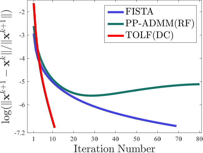
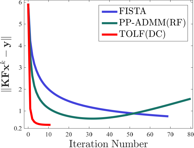
We also compared the iteration behaviors of FISTA, PP-ADMM and TOLF in Fig. 2. For the last two methods, we only chose the inner operator $\mathcal{T}$ with better performances in Table II (i.e., RF for PP-ADMM and DC for TOLF) to provide clearer illustrations. We observed that the speed of FISTA was slow and the iterations converged after 70 steps. It also can be seen that PP-ADMM (RF) did not converge even after 80 steps, but it obtained lower reconstruction errors than FISTA near the 30th step (see the right subfigure). In contrast, TOLF (DC) converged only after 10 iterations and achieved the lowest reconstruction errors.

Next, we adopted some recently proposed non-convex regularization techniques [17, 19] (e.g., replace $\ell_{1}$-norm by $\ell_{p}$-norm, $p=0,0.5,0.8$) to reformulate Eq. (9) for image restoration. The same non-convex accelerated proximal gradient scheme [20] was performed to solve these $\ell_{p}$-regularized models. Their iteration behaviors are visualized in Fig. 3. We also plotted the iteration curves of FISTA and our TOLF on the original $\ell_{1}$-norm regularized model in this figure. It can be seen that these non-convex regularization models improved the practical performance (i.e., PSNR in the right subfigure) of the original convex model in Eq. (9) (solved by FISTA, denoted as $\ell_{1}$), but their trajectories fluctuated after several iterations (see the left subfigure). In contrast, TOLF obtained the fastest convergence speed and the best final performance among all the compared methods, even by only solving a convex model.

Finally, we presented numerical results and iterative behaviors in terms of the compound regularization (i.e., $\min_{\mathbf{x}}F(\mathbf{x})+\lambda\Psi(\mathbf{x})$, where $\lambda$ is the positive balancing parameter) and our model (i.e., $\min_{\mathbf{x}}F(\mathbf{x})\;\;s.t.\ \mathbf{x}\in\arg\min_{\mathbf{x}}\Psi(\mathbf{x})$). To ensure fairness, we adopted the proximal ADMM (used for our TOLF) to solve the model of compound regularization. In addition, we considered the same $\mathcal{T}$ to define $\mathbf{u}$ in $\Psi(\mathbf{x})$. As presented in Table II, we recognized that DC (deconvolution process) is a crucial step for obtaining $\mathbf{u}$, so we would like to emphasize that we performed DC before denoising operation (e.g., RF, and DnCNN [45]) in the following experiments. Table III reported quantitative results of these two models by adopting different settings. Note that $\lambda=0.1$ in the compound regularization. Thanks to our newly-introduced latent feasibility, it can be easily seen that our results were consistently superior to compound regularization in all cases. The fact that the quantitative scores of TOLF (RF^∗) (32.22/0.9103) obtained a significant improvement than TOLF (RF) (30.95/0.8871) (^∗ represents that DC is performed before denoising), also justified the necessity of the task-specific operation for T. Fig. 4 displayed iteration behaviors of compound regularization and our TOLF. To make a rigorous evaluation, we change settings of compound regularization by adopting different $\lambda$. We can easily observe that with the value of $\lambda$ decreasing, the compound regularization converged more slowly but obtained better performance. By contrast, our TOLF realized a higher value at a faster speed than all naive compound regularizations with different regularization parameters. This experiment indicates that compound regularization cannot promote numerical improvement and accelerate the convergence speed simultaneously, while TOLF we proposed can obtain a satisfying outcome.

The proposed algorithm involves many parameters as described in Sec. V-B, some of which are iteration variables introduced based on the proximal ADMM scheme, i.e., $\lambda_{\mathbf{x}},\lambda_{\mathbf{z}},\lambda_{{\mathbf{s}_{1}}},\lambda_{\mathbf{s}_{2}},\lambda_{r}$. As for them, we followed the commonly-used setting (set as zero) to initialize them. Here we mainly explored the effects of some algorithmic parameters including $\tau,\zeta$, and $\beta$. As shown in Fig. 5, $\tau$ and $\zeta$ were insensitive to different settings to some extent, while the parameter $\beta$ was sensitive when it increased. Large $\beta$ caused poor performance. Additionally, based on these results, we defined $\tau=15$, $\zeta=1$, $\beta=0.1$ as our default settings for solving image restoration.

Table IV reported quantitative scores of using different networks for PP-ADMM and our method. Among them, TNRD [47] is a famous image denoising framework based on a nonlinear reaction-diffusion model; DnCNN [45] is a well-known CNN-based network for image denoising; IRCNN is a recently-proposed plug-and-play framework for image restoration, and here we just utilized its denoising architecture. It can be easily seen that DnCNN reached the highest scores both in PP-ADMM and our method because it owned stronger denoising ability than IRCNN and TNRD. Thus we chose DnCNN as $\mathcal{T}$ for image restoration in the experiments mentioned above and in the following experiments. Moreover, the results of our method were consistently better than PP-ADMM under different networks. It showed the superiority of our designed computational framework against the classical PP-ADMM after plugging the learnable architecture.

Image Restoration. We compared TOLF with many approaches, including traditional optimization methods (i.e., FTVd [2], FISTA [1], HL [17], IDDBM3D [48], EPLL [16]), and learning-based methods (i.e., MLP [49], IRCNN [6], MSWNNM [50], FDN [51], GLRA [52], PP-ADMM [24], MEDAEP [53], FIMA [7] (contains eFIMA and iFIMA)). As for TOLF, we introduced a denoising CNN [45] architecture as $\mathcal{T}$ (according to Table IV). We conducted experiments on the Levin et al.’ benchmark [44], which includes 32 images of the size 255$\times$255 and blurred by 8 different kernels of the size ranging from 13$\times$13 to 27$\times$27. We reported the quantitative scores in Table V. The visual comparisons on an example image from this benchmark were plotted in Fig. 6. Obviously, deep-learning-based IRCNN achieved much better performance than other traditional optimization methods. The recently-proposed FIMA (includes eFIMA and iFIMA) considered integrating the data and knowledge by an optimization unrolling strategy, thus its results were even better. Nevertheless, thanks to the novel modeling mechanism, TOLF obtained the best quantitative and qualitative results. In addition, a color image (612$\times$342) corrupted by a very large kernel (75$\times$75) was used to further evaluate the performance, shown in Fig. 7. Again, TOLF recovered richer textures and details, and thus performed the best.

Compressed Sensing MRI (CS-MRI). We then evaluated TOLF on the CS-MRI task. Here we defined the task-specific operation $\arg\min_{\mathbf{x}}\|\mathbf{PHF}\mathbf{x}-\mathbf{y}\|^{2}+\alpha\|\mathbf{Fx}-\mathbf{y}\|^{2}$ with a trade-off $\alpha>0$ (fix it as $10^{-3}$) and the pre-trained denoising model described in [6] together as $\mathcal{T}$. Specifically, we conducted experiments on 55 images from the widely-used IXI MRI benchmark⁵⁵ 5 http://brain-development.org/ixi-dataset/.. Our experiments contained three types of undersampling patterns (i.e., Cartesian, Gaussian, and Radial mask) and two sampling rates (i.e., 20$\%$, 30$\%$) to generate the sparse $k$-space data. We compared TOLF with many state-of-the-art methods including TV [54], SIDWT [55], PBDW [56], PANO [57], FDLCP [58], ADMM-Net [59], TGDOF [9], and BM3D-MRI [60]. Fig. 8 illustrated the quantitative results of these approaches on the test dataset. Our TOLF achieved the best results according to both PSNR and SSIM scores (i.e., the upper right red points). At a sampling rate of 30%, Fig. 10 demonstrated CS-MRI results on a challenging chest data [9] with Cartesian mask. Obviously, TOLF obtained the best quantitative and qualitative performance.

Low-Light Image Enhancement (LLIE). Lastly, we applied TOLF to solve LLIE. Here we defined the task-specific operation as $\mathbf{x}=\mathbf{y}\oslash\mathcal{T}(\mathbf{y})$, where $\oslash$ represents the element-wise division. We compared TOLF with two optimization methods (i.e., JIEP [61] and RRM [11]) and two recent deep learning techniques (i.e., LightenNet [62] and DeepUPE [46]). Fig. 12 illustrated the visual results of these methods on two challenging images. Quantitative results were reported in Fig. 13. By comparison, TOLF obtained the best visual quality and the highest scores. In Fig. 14, we compared the performance of TOLF with different warm-start operations $\mathcal{T}$, including the naive low-light input (denoted as $\mathbf{y}$), the result of the gamma correction (denoted as $\mathbf{y}^{{1}/{a}}$ with $a=2.2$), a simplified relative total variation filter [18] (denoted as $\mathtt{RTV}(\mathbf{y}))$, and the simple denoising CNN architecture used in the above image restoration experiment (denoted as $\mathtt{CNN}(\mathbf{y})$). We first observed that TOLF with $\mathtt{RTV}$ and $\mathtt{CNN}$ performed better than the other two choices. On the other hand, we emphasize that even with different warm starts, the TOLF process consistently improved the overall performance.

References

- [1] A. Beck and M. Teboulle, “A fast iterative shrinkage-thresholding algorithm for linear inverse problems,” SIAM Journal on Imaging Sciences, vol. 2, no. 1, pp. 183–202, 2009.
- [2] C. Li, W. Yin, H. Jiang, and Y. Zhang, “An efficient augmented lagrangian method with applications to total variation minimization,” Computational Optimization and Applications, vol. 56, no. 3, pp. 507–530, 2013.
- [3] X. Peng, J. Feng, S. Xiao, W.-Y. Yau, J. T. Zhou, and S. Yang, “Structured autoencoders for subspace clustering,” IEEE Transactions on Image Processing, vol. 27, no. 10, pp. 5076–5086, 2018.
- [4] Z. Huang, P. Hu, J. T. Zhou, J. Lv, and X. Peng, “Partially view-aligned clustering,” Advances in Neural Information Processing Systems, vol. 33, 2020.
- [5] J. Bolte, S. Sabach, and M. Teboulle, “Proximal alternating linearized minimization for nonconvex and nonsmooth problems,” Mathematical Programming, vol. 146, no. 1-2, pp. 459–494, 2014.
- [6] K. Zhang, W. Zuo, S. Gu, and L. Zhang, “Learning deep cnn denoiser prior for image restoration,” in Proceedings of the IEEE Conference on Computer Vision and Pattern Recognition, 2017, pp. 3929–3938.
- [7] R. Liu, S. Cheng, Y. He, X. Fan, Z. Lin, and Z. Luo, “On the convergence of learning-based iterative methods for nonconvex inverse problems,” IEEE Transactions on Pattern Analysis and Machine Intelligence, vol. 42, no. 12, pp. 3027–3039, 2019.
- [8] R. Liu, P. Mu, J. Chen, X. Fan, and Z. Luo, “Investigating task-driven latent feasibility for nonconvex image modeling,” IEEE Transactions on Image Processing, vol. 29, pp. 7629–7640, 2020.
- [9] R. Liu, Y. Zhang, S. Cheng, X. Fan, and Z. Luo, “A theoretically guaranteed deep optimization framework for robust compressive sensing mri,” in Association for the Advancement of Artificial Intelligence, 2019.
- [10] S. Bubeck et al., “Convex optimization: Algorithms and complexity,” Foundations and Trends® in Machine Learning, vol. 8, no. 3-4, pp. 231–357, 2015.
- [11] M. Li, J. Liu, W. Yang, X. Sun, and Z. Guo, “Structure-revealing low-light image enhancement via robust retinex model,” IEEE Transactions on Image Processing, vol. 27, no. 6, pp. 2828–2841, 2018.
- [12] S. Dempe, V. Kalashnikov, G. A. Prez-Valds, and N. Kalashnykova, Bilevel Programming Problems: Theory, Algorithms and Applications to Energy Networks. Springer Publishing Company, Incorporated, 2015.
- [13] R. Tibshirani, “Regression shrinkage and selection via the lasso,” Journal of the Royal Statistical Society: Series B (Methodological), vol. 58, no. 1, pp. 267–288, 1996.
- [14] E. J. Candès and B. Recht, “Exact matrix completion via convex optimization,” Foundations of Computational mathematics, vol. 9, no. 6, p. 717, 2009.
- [15] S. Boyd and L. Vandenberghe, Convex optimization. Cambridge university press, 2004.
- [16] D. Zoran and Y. Weiss, “From learning models of natural image patches to whole image restoration,” in Proceedings of the IEEE Conference on Computer Vision and Pattern Recognition, 2011, pp. 479–486.
- [17] D. Krishnan and R. Fergus, “Fast image deconvolution using hyper-laplacian priors,” in Neural Information Processing Systems, 2009, pp. 1033–1041.
- [18] L. Xu, Q. Yan, Y. Xia, and J. Jia, “Structure extraction from texture via relative total variation,” ACM Transactions on Graphics, vol. 31, no. 6, 2012.
- [19] J. Pan, Z. Hu, Z. Su, and M.-H. Yang, “-regularized intensity and gradient prior for deblurring text images and beyond,” IEEE Transactions on Pattern Analysis and Machine Intelligence, vol. 39, no. 2, pp. 342–355, 2016.
- [20] H. Li and Z. Lin, “Accelerated proximal gradient methods for nonconvex programming,” in Neural Information Processing Systems, 2015, pp. 379–387.
- [21] P. Jain, P. Kar et al., “Non-convex optimization for machine learning,” Foundations and Trends® in Machine Learning, vol. 10, no. 3-4, pp. 142–336, 2017.
- [22] S. N. Negahban, P. Ravikumar, M. J. Wainwright, B. Yu et al., “A unified framework for high-dimensional analysis of -estimators with decomposable regularizers,” Statistical Science, vol. 27, no. 4, pp. 538–557, 2012.
- [23] Y. Chen and M. J. Wainwright, “Fast low-rank estimation by projected gradient descent: General statistical and algorithmic guarantees,” arXiv preprint arXiv:1509.03025, 2015.
- [24] S. H. Chan, X. Wang, and O. A. Elgendy, “Plug-and-play admm for image restoration: Fixed-point convergence and applications,” IEEE Transactions on Computational Imaging, vol. 3, no. 1, pp. 84–98, 2016.
- [25] Y. Romano, M. Elad, and P. Milanfar, “The little engine that could: Regularization by denoising,” SIAM Journal on Imaging Sciences, vol. 10, no. 4, pp. 1804–1844, 2017.
- [26] W. Dong, P. Wang, W. Yin, G. Shi, F. Wu, and X. Lu, “Denoising prior driven deep neural network for image restoration,” IEEE Transactions on Pattern Analysis and Machine Intelligence, vol. 41, no. 10, pp. 2305–2318, 2018.
- [27] E. Ryu, J. Liu, S. Wang, X. Chen, Z. Wang, and W. Yin, “Plug-and-play methods provably converge with properly trained denoisers,” in International Conference on Machine Learning, 2019, pp. 5546–5557.
- [28] S. Sreehari, S. V. Venkatakrishnan, B. Wohlberg, G. T. Buzzard, L. F. Drummy, J. P. Simmons, and C. A. Bouman, “Plug-and-play priors for bright field electron tomography and sparse interpolation,” IEEE Transactions on Computational Imaging, vol. 2, no. 4, pp. 408–423, 2016.
- [29] A. M. Teodoro, J. M. Bioucas-Dias, and M. A. Figueiredo, “A convergent image fusion algorithm using scene-adapted gaussian-mixture-based denoising,” IEEE Transactions on Image Processing, vol. 28, no. 1, pp. 451–463, 2018.
- [30] Y. Sun, B. Wohlberg, and U. S. Kamilov, “An online plug-and-play algorithm for regularized image reconstruction,” IEEE Transactions on Computational Imaging, vol. 5, no. 3, pp. 395–408, 2019.
- [31] Y. Sun, Z. Wu, X. Xu, B. Wohlberg, and U. S. Kamilov, “Scalable plug-and-play admm with convergence guarantees,” IEEE Transactions on Computational Imaging, vol. 7, pp. 849–863, 2021.
- [32] E. T. Reehorst and P. Schniter, “Regularization by denoising: Clarifications and new interpretations,” IEEE Transactions on Computational Imaging, vol. 5, no. 1, pp. 52–67, 2018.
- [33] P. Nair, R. G. Gavaskar, and K. N. Chaudhury, “Fixed-point and objective convergence of plug-and-play algorithms,” IEEE Transactions on Computational Imaging, vol. 7, pp. 337–348, 2021.
- [34] R. Cohen, M. Elad, and P. Milanfar, “Regularization by denoising via fixed-point projection (red-pro),” SIAM Journal on Imaging Sciences, vol. 14, no. 3, pp. 1374–1406, 2021.
- [35] R. G. Gavaskar, C. D. Athalye, and K. N. Chaudhury, “On plug-and-play regularization using linear denoisers,” IEEE Transactions on Image Processing, vol. 30, pp. 4802–4813, 2021.
- [36] X. Xu, Y. Sun, J. Liu, B. Wohlberg, and U. S. Kamilov, “Provable convergence of plug-and-play priors with mmse denoisers,” IEEE Signal Processing Letters, vol. 27, pp. 1280–1284, 2020.
- [37] M. Solodov, “An explicit descent method for bilevel convex optimization,” Journal of Convex Analysis, vol. 14, no. 2, p. 227, 2007.
- [38] A. Beck and S. Sabach, “A first order method for finding minimal norm-like solutions of convex optimization problems,” Mathematical Programming, vol. 147, no. 1-2, pp. 25–46, 2014.
- [39] S. Sabach and S. Shtern, “A first order method for solving convex bilevel optimization problems,” SIAM Journal on Optimization, vol. 27, no. 2, pp. 640–660, 2017.
- [40] A. L. Dontchev and R. T. Rockafellar, “Implicit functions and solution mappings,” Springer Monographs in Mathematics. Springer, vol. 208, 2009.
- [41] J. Eckstein and D. P. Bertsekas, “On the Douglas-Rachford splitting method and the proximal point algorithm for maximal monotone operators,” Mathematical Programming, vol. 55, no. 1, pp. 293–318, 1992.
- [42] S. Boyd, N. Parikh, and E. Chu, Distributed optimization and statistical learning via the alternating direction method of multipliers. Now Publishers Inc, 2011.
- [43] J. M. Bioucas-Dias and M. A. Figueiredo, “A new twist: two-step iterative shrinkage/thresholding algorithms for image restoration,” IEEE Transactions on Image Processing, vol. 16, no. 12, pp. 2992–3004, 2007.
- [44] A. Levin, Y. Weiss, F. Durand, and W. T. Freeman, “Understanding and evaluating blind deconvolution algorithms,” in Proceedings of the IEEE Conference on Computer Vision and Pattern Recognition, 2009, pp. 1964–1971.
- [45] K. Zhang, W. Zuo, Y. Chen, D. Meng, and L. Zhang, “Beyond a gaussian denoiser: Residual learning of deep cnn for image denoising,” IEEE Transactions on Image Processing, vol. 26, no. 7, pp. 3142–3155, 2017.
- [46] R. Wang, Q. Zhang, C.-W. Fu, X. Shen, W.-S. Zheng, and J. Jia, “Underexposed photo enhancement using deep illumination estimation,” in Proceedings of the IEEE Conference on Computer Vision and Pattern Recognition, 2019, pp. 6849–6857.
- [47] Y. Chen and T. Pock, “Trainable nonlinear reaction diffusion: A flexible framework for fast and effective image restoration,” IEEE Transactions on Pattern Analysis and Machine Intelligence, vol. 39, no. 6, pp. 1256–1272, 2016.
- [48] A. Danielyan, V. Katkovnik, and K. Egiazarian, “Bm3d frames and variational image deblurring,” IEEE Transactions on Image Processing, vol. 21, no. 4, pp. 1715–1728, 2012.
- [49] C. J. Schuler, H. C. Burger, S. Harmeling, and B. Scholkopf, “A machine learning approach for non-blind image deconvolution,” in Proceedings of the IEEE Conference on Computer Vision and Pattern Recognition, 2013, pp. 1067–1074.
- [50] N. Yair and T. Michaeli, “Multi-scale weighted nuclear norm image restoration,” in Proceedings of the IEEE Conference on Computer Vision and Pattern Recognition, 2018, pp. 3165–3174.
- [51] J. Kruse, C. Rother, and U. Schmidt, “Learning to push the limits of efficient fft-based image deconvolution,” in Proceedings of the IEEE International Conference on Computer Vision, 2017, pp. 4586–4594.
- [52] W. Ren, J. Zhang, L. Ma, J. Pan, X. Cao, W. Zuo, W. Liu, and M.-H. Yang, “Deep non-blind deconvolution via generalized low-rank approximation,” in Advances in Neural Information Processing Systems, 2018, pp. 297–307.
- [53] S. Li, B. Qin, J. Xiao, Q. Liu, Y. Wang, and D. Liang, “Multi-channel and multi-model-based autoencoding prior for grayscale image restoration,” IEEE Transactions on Image Processing, vol. 29, pp. 142–156, 2019.
- [54] M. Lustig, D. L. Donoho, J. M. Santos, and J. M. Pauly, “Compressed sensing mri,” IEEE Signal Processing Magazine, vol. 25, no. 2, pp. 72–82, 2008.
- [55] R. G. Baraniuk, “Compressive sensing [lecture notes],” IEEE Signal Processing Magazine, vol. 24, no. 4, pp. 118–121, 2007.
- [56] X. Qu, D. Guo, B. Ning, Y. Hou, Y. Lin, S. Cai, and Z. Chen, “Undersampled mri reconstruction with patch-based directional wavelets,” Magnetic Resonance Imaging, vol. 30, no. 7, pp. 964–97, 2012.
- [57] X. Qu, Y. Hou, F. Lam, D. Guo, J. Zhong, and Z. Chen, “Magnetic resonance image reconstruction from undersampled measurements using a patch-based nonlocal operator,” Medical Image Analysis, vol. 18, no. 6, pp. 843–856, 2014.
- [58] Z. Zhan, J.-F. Cai, D. Guo, Y. Liu, Z. Chen, and X. Qu, “Fast multiclass dictionaries learning with geometrical directions in mri reconstruction,” IEEE Transactions on Biomedical Engineering, vol. 63, no. 9, pp. 1850–1861, 2016.
- [59] Y. Yang, J. Sun, H. Li, and Z. Xu, “Admm-csnet: A deep learning approach for image compressive sensing,” IEEE Transactions on Pattern Analysis and Machine Intelligence, 2018.
- [60] E. M. Eksioglu, “Decoupled algorithm for mri reconstruction using nonlocal block matching model: Bm3d-mri,” Journal of Mathematical Imaging and Vision, vol. 56, no. 3, pp. 430–440, 2016.
- [61] B. Cai, X. Xu, K. Guo, K. Jia, B. Hu, and D. Tao, “A joint intrinsic-extrinsic prior model for retinex,” in International Conference on Computer Vision, 2017.
- [62] C. Li, J. Guo, F. Porikli, and Y. Pang, “Lightennet: a convolutional neural network for weakly illuminated image enhancement,” Pattern Recognition Letters, vol. 104, pp. 15–22, 2018.
- [63] B. He, L.-Z. Liao, D. Han, and H. Yang, “A new inexact alternating directions method for monotone variational inequalities,” Mathematical Programming, vol. 92, no. 1, pp. 103–118, 2002.
- [64] X. Yuan, S. Zeng, and J. Zhang, “Discerning the linear convergence of admm for structured convex optimization through the lens of variational analysis.” Journal of Machine Learning Research, vol. 21, pp. 83–1, 2020.
![[Uncaptioned image]](1907.03083v2/LiuRisheng.png) |
Risheng Liu (M’12-) received the BSc and PhD degrees both in mathematics from the Dalian University of Technology in 2007 and 2012, respectively. He was a visiting scholar in the Robotic Institute of Carnegie Mellon University from 2010 to 2012. He served as Hong Kong Scholar Research Fellow at the Hong Kong Polytechnic University from 2016 to 2017. He is currently a professor with the International School of Information Science & Engineering, Dalian University of Technology. His research interests include machine learning, optimization, computer vision and multimedia. He was a co-recipient of the IEEE ICME Best Student Paper Award in both 2014 and 2015. Two papers were also selected as Finalist of the Best Paper Award in ICME 2017. He is a member of the IEEE and ACM. |
![[Uncaptioned image]](1907.03083v2/MaLong.png) |
Long Ma received the M.S. degree in software engineering at Dalian University of Technology, Dalian, China, in 2019. He is currently pursuing the Ph. D. degree in software engineering at Dalian University of Technology, Dalian, China. His research interests include computer vision, image enhancement and machine learning. He is a reviewer for CVPR, ICCV, AAAI, ACCV, IEEE TCSVT, and Neurocomputing. |
![[Uncaptioned image]](1907.03083v2/YuanXiaoming.png) |
Xiaoming Yuan is Professor at Department of Mathematics, The University of Hong Kong. His main research interests include numerical optimization, scientific computing and optimal control. Recently, he is particularly interested in optimization problems in various AI and cloud computing areas. |
![[Uncaptioned image]](1907.03083v2/ZengShangzhi.png) |
Shangzhi Zeng received the B.Sc. degree in Mathematics and Applied Mathematics from Wuhan University in 2015, the M.Phil. degree from Hong Kong Baptist University in 2017, and the Ph.D. degree from the University of Hong Kong in 2021. He is currently a PIMS postdoctoral fellow in the Department of Mathematics and Statistics at University of Victoria. His current research interests include variational analysis and bilevel optimization. |
![[Uncaptioned image]](1907.03083v2/ZhangJin.png) |
Jin Zhang received the B.A. degree in Journalism from the Dalian University of Technology in 2007. He pursued a degree in mathematics and received the M.S. degree in Operational Research and Cybernetics from the Dalian University of Technology, China, in 2010, and the Ph. D. degree in Applied Mathematics from University of Victoria, Canada, in 2015. After working in Hong Kong Baptist University for 3 years, he joined Southern University of Science and Technology as a tenure-track assistant professor in the department of mathematics. His broad research area is comprised of optimization, variational analysis and their applications in economics, engineering and data science. |