Estimation of spatio-temporal wave grouping properties using Delaunay triangulation and spline techniques
Abstract
Wave groups can be detected and studied by using the wave envelope. So far, the method used to compute the wave envelope employs the Riesz transform. However, such a technique always produces symmetric envelopes, which is only realistic in the case of linear waves. In this paper we present a new method to compute the wave envelope providing more realistic results. In particular, the method allows to detect non-symmetry in the wave envelope, something useful, for instance, when detecting groups of high waves. The method computes first the local maxima and minima of the sea surface, and then determines the wave envelope by combining discrete methods, namely the use of the Delaunay triangulation, and tensor-product splines. The proposed method has been applied to simulated wave fields, and also to wave elevations data measured by an X-band radar. The obtained results correctly reproduce the behavior of the simulated waves.
Keywords: wave envelope, wave field, Delaunay triangulation, spline methods.
1 Introduction
Ocean gravity waves propagate in the ocean as packages of consecutive high waves traveling together [36, 37]. This phenomenon is known in the literature as wave grouping [45, 25]. Those wave groups are specially dangerous for marine activities, such as navigation, coastal management, on- and off-shore platform operation, etc. This danger is not only caused by the presence of high waves, but also by the fact that those waves propagate with nearly equal periods, which can produce stability problems to marine structures when the wave periods involved in the groups are close to the resonant period of the structure, such as moving vessels, breakwaters, etc. [45, 7].
Although the analysis of wave grouping has been carried out for several decades [27, 41, 32], this phenomenon and its properties are not fully explained yet [45], and, therefore, it needs to be analyzed in detail for a better understanding of the dynamical mechanisms involved in the wave group propagation, such as the persistence of the groups, number of waves within a group, etc.
Wave grouping has been studied traditionally in the temporal domain by using wave elevation time series acquired by in situ-sensors (e.g., anchored buoys, pressure gauges, wave lasers, etc.). Hence, those measurements can characterize wave grouping features at a fixed position (i.e., the point of deployment) [39, 12]. Alternatively to those point measurements, in recent years different remote imaging techniques capable of studying the sea surface in space and time have been developed. Some of these techniques are based on the use of passive sensors, like video cameras [47, 20, 2, 49]. Other techniques use active microwave sensors, such as incoherent and coherent radars mounted on off- and on-shore stations or moving vessels [57, 6, 4, 5, 42, 54, 58, 9, 3, 56, 51]. All those remote sensing techniques are able to acquire temporal sequences of images of the sea surface. The spatio-temporal information provides a more detailed description of the wave elevation properties than the historical measurements based on time series analysis and, therefore, it requires the use of additional tools, or even new techniques of analysis, to obtain information of the wave field evolution in space and time [35].
In one-dimensional records (i.e., wave elevation data depending on only one parameter, such as heave time series measured by a buoy), the individual wave heights can be estimated by applying the zero-up crossing method, or similar techniques, but those methods are difficult to extend to a higher number of dimensions. A way to study the spatio-temporal evolution of wave heights and groups consists of the estimation of the wave envelope depending on the variables . For linear and narrow-banded wave fields the envelope can be estimated by the Riesz Transform (RT) [44], which is a multidimensional generalization of the Hilbert transform (HT)[33]. For nonlinear andor broadband wave fields RT, or HT for time series, is not the appropriate solution. The reason is that the RT always leads symmetry between the upper and the lower envelopes [33, 44]. Furthermore, the narrowband hypothesis reduces the irregularity of the envelope passing through most of the local maxima, and the local minima for the case of the lower envelope [45]. This is accurate for linear wave fields, but not for non-linear wave fields, where there may be asymmetries between wave crests and wave troughs with respect to the mean sea level. We argue this in more detail in Section 2.
Therefore, other techniques should be applied. An example of an alternative technique appears in [50], where the authors reconstruct the two-dimensional envelope of nonlinear wave fields by applying sets of one-dimensional splines parallel to the mean wave propagation direction in the -domain for different time steps . The approach that we present in this paper also makes use of splines, but proceeds in a completely different way to that in [50]. The main idea is to use two-dimensional spline interpolation, to refine a first (linear) approximation of the envelope computed by using discrete methods, namely Delaunay triangulation [10, 19].
In more detail, for a fixed time our method first locates the wave points corresponding to local positive maxima and local negative minima of the wave elevation function, by comparing the elevation of each point with the elevations of its immediate neighbours. Then, we use the Delaunay triangulation to build a piecewise-linear model of the envelope. Finally, we refine this model by using tensor-product spline interpolation [38, 46] This refinement step is necessary, because the linear approximation introduces fictitious harmonics and spectral noise, which however disappear when the spline refinement is applied. Therefore, while the method in [50] uses one-dimensional splines to build slices of the wave envelope surface, we directly build the surface in one go, considering the two-dimensional structure of the sea surface.
The method proposed in this paper is suitable both for linear and non-linear wave fields, and has been used for different simulated wave elevation fields using the standard stochastic approach of linear wave fields and a second-order nonlinear approach based on the model proposed by [52] [43].
The paper is structured as follows: Section 2 describes the properties of the envelope derived from RT for linear wave fields. Section 3 describes the mathematical techniques used in the method, namely triangulations and tensor-product spline interpolation, as well as the method itself. Section 4 deals with a brief description of the wave field simulation methods (i.e. linear and second-order approach stochastic models) used in this paper, as well as the corresponding results obtained for the estimation of the related wave grouping properties. Section 5 addresses the effect of measurement errors in the method. In Section 6, the method is applied to a wave elevation map measured by an X-band radar mounted at the German platform FINO 1, located on the North Sea. Finally, Section 7 summarizes our conclusions.
2 Spatio-temporal wave envelope for linear and narrow-banded wave fields
Under the frame of the linear wave theory, the wave elevation field , where , is regarded as a superposition of different monochromatic wave components [45], where each component is characterized by its amplitude , wave number vector , angular frequency , and phase . Hence, using a discrete notation, can be expressed as
| (1) |
Eq. 1 corresponds to an Eulerian description of the wave elevation process [34], where wave numbers and frequencies are dependent through the dispersion relation for linear gravity waves (i.e., , being , the acceleration of the gravity and the water depth). Those wave fields given by (1) are considered as zero-mean Gaussian stochastic processes, where the spectral components are statistically independent, being and random variables, which are statistically homogeneous in space and stationary in time [25]. Under these conditions, and taking into account (1), the variance of is
| (2) |
where denotes the expectation operator. Note that Eq. 2 considers . As Eq. 1 represents a Gaussian process, this model describes wave fields with statistical symmetry between wave crests and troughs [45].
2.1 Spatio-temporal estimation of the wave envelope by using the Riesz Transform
In a similar way that is done for wave elevation time series [25], assuming that the process is linear narrow-banded [45], the spatio-temporal description of linear wave elevation fields can be factorized using the so-called local and instantaneous amplitude and local and instantaneous phase as [44]
| (3) |
The spatio-temporal wave grouping properties are described from the local and instantaneous amplitude [44]. In the development of (3), it is assumed that the wave field is described by a characteristic wave number and frequency, which can be understood as the carrier of the process [25]. This fact is a consequence of the narrow-band approach and the assumption of the linear wave theory [45]. Furthermore, (3) indicates that , being and the so-called lower and upper envelope respectively [44]. Those magnitudes are denoted in this paper as , and . It can be seen that the model described by (3) has symmetric lower and upper envelopes (i.e. ), This is a consequence of the linearity assumption but not of the narrowband approach. Under these conditions, the wave height is regarded as twice the amplitude [25]. However, for non-linear wave fields, where there may be asymmetries between wave crests and wave troughs with respect to the mean sea level, the upper and lower envelopes are not symmetric either (i.e. ). For those cases, equation (3) has some limitations to describe the wave grouping phenomenon.
For those cases where the hypothesis of (3) holds, the local and instantaneous wave envelope may be estimated by the Riesz Transform (RT) [44], which is a multidimensional generalization of the Hilbert Transform used for wave grouping analysis of wave elevation time series [39]. For a given time , the two-dimensional RT of the wave elevation field is defined as [33]
| (4) |
where . The index takes the values or denoting the directions and respectively. Note that RT has two components in this particular case, , and . From the two components of RT a vector field is constructed as [33]
| (5) |
The estimation of the local and instantaneous amplitude is obtained as the norm of the vector field
| (6) |
The respective RT estimation of the local and instantaneous phase is given by
| (7) |
For practical cases, (4) is not applied and RT is computed by using the relationship between the Fourier transforms of the original signal and its respective RT vector components [33, 44]
| (8) |
where denotes the two-dimensional Fourier Transform from the spatial to the wave number domain () for a given fixed time , while and are the two components of the wave number vector . Taking into account the linear wave field described by (1), the two components of RT given by (8) are
| (9) | |||||
| (10) |
where is the propagation direction of the spectral component. Therefore, , and , which are related with the transfer functions of RT given by Equation 8. Equations 9 and 10 are the horizontal Lagrangian wave displacements at the mean sea level () of the wave elevation field given by Eq. 1 [34, 44]. Hence, the local and instantaneous wave envelope can be understood as the norm of the vector field , whose components are the wave elevation and the horizontal wave displacements in a single wave cycle. The expectation of defined in (6) is twice the variance of
| (11) |
2.1.1 Spectral components of the envelope derived from RT
The location of the spectral components of the envelope can be identified considering in (6) together with (1), (9), and (10) for , , and respectively. Thus,
| (12) |
where, using the definition , the terms and are given by
| (13) |
| (14) |
From (13) and (14), it can be seen that the spectral components of correspond to second-order differences of the spectral variables, , , while has second-order summation components , . Therefore, is responsible for the long scale spatio-temporal evolution (long distances and slow times), and of the short scale spatio-temporal changes (short distances and fast times). The magnitude is commonly known in the literature as group train, and as pulse train [21]. Taking into account that the spectral components of the wave field are statistically independent, the expectation operator applied to (13) and (14) is
| (15) | |||||
| (16) |
The group train is responsible of the wave energy propagation as the mean value of the pulse train vanishes [44]. Assuming the existence of a dispersion relation , the “phase speed” of the spectral component of is
| (18) |
which is the group velocity of the wave field components. As an example, Fig. 1 shows a simulated linear wave field (left) depending on the sea surface coordinates at a fixed time , and its amplitude estimation derived from RT (right). Their wave number and frequency spectra are illustrated in Fig. 2. The spectrum of the envelope can be seen on the right part of that figure, where the spectral components of the group and pulse trains can be identified.
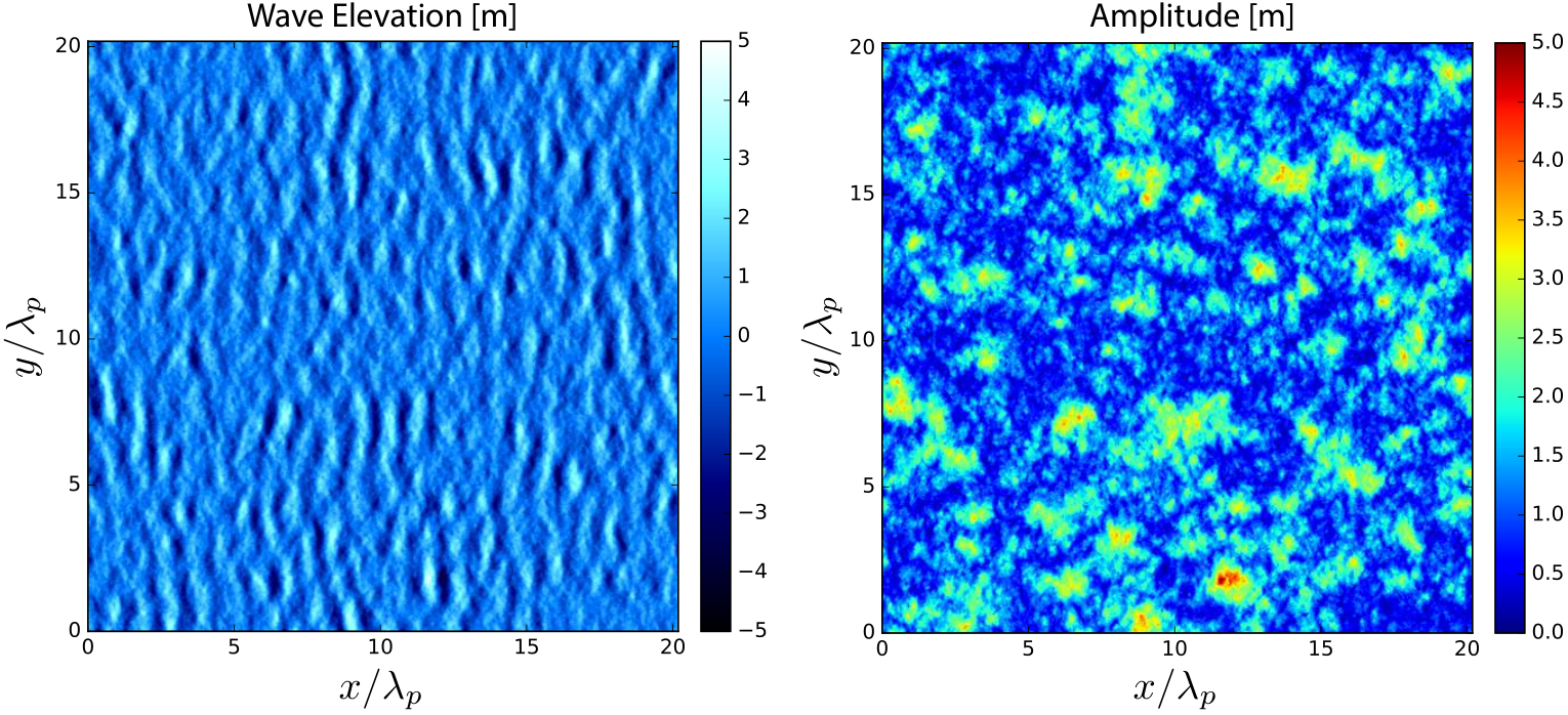
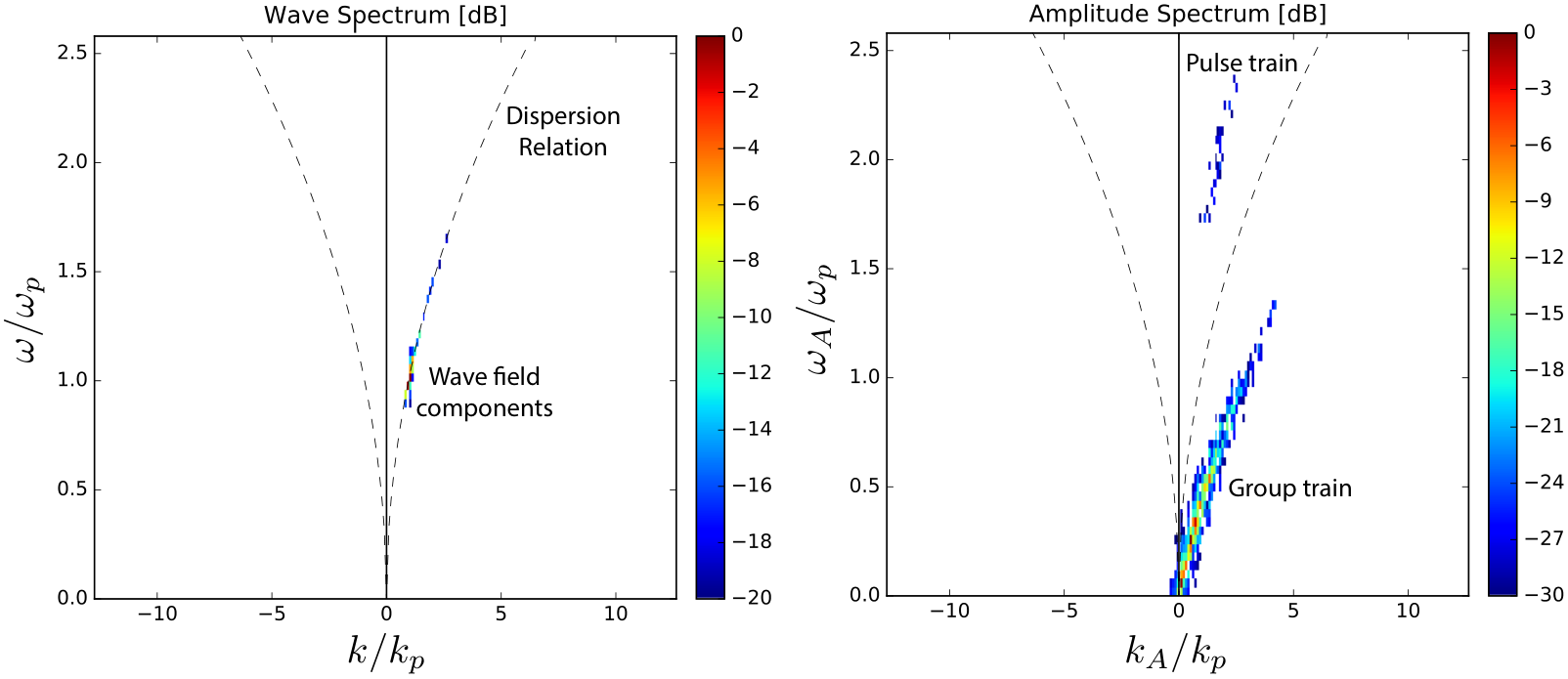
Taking into account (15) and (18), the relevant magnitude to analyze the spatio-temporal properties of wave grouping is the group train rather than the pulse train . Therefore, as evolves in very short scales of distances and times, its contribution adds noise in the envelope for the wave grouping study. This effect is well known for time series analysis of wave groups derived from buoy records [36, 37]. In that case, the estimation of the envelope derived from HT is applied to wave elevation time series previously filtered with a band-pass filter centered in the peak frequency . This method is difficult to generalize to higher number of dimensions, as the -domain. Therefore, an alternative estimation method of the spatio-temporal envelope, without the need of applying any kind of additional filter, would be more useful. In addition, as it has already been mentioned, RT provides symmetric upper and lower envelopes, which are not representative of linear or not-narrow-banded wave fields. Thus, for any kind of wave field, it is necessary to use different approaches that permit the estimation of independent smooth upper and lower envelope that pass through all the local maxima (crests) and minima (troughs) respectively. The following section deals with the description of the techniques proposed in this paper to estimate the envelopes, based on discrete and spline methods.
3 Estimation of wave envelopes using discrete and spline methods
In this section we present an alternative mathematical method to construct the upper and lower wave envelopes. Here we assume that we have measured the wave elevations at a given time , at several points , with and , of a rectangular grid, see Fig. 3. Furthermore, we will denote by the elevation at the point . The method consists of three steps (we will later refer to these steps as Step 1, Step 2 and Step 3):
- 1.
First (Section 3.1), we search for the positions in corresponding to local maxima and local minima of the surface ; keeping only the set of local maxima with positive , denoted by , and the set of local minima with negative , denoted by .
- 2.
Second (Section 3.2), we appropriately connect the points to compute a piecewise-linear, i.e., polyhedral, surface which approximates the upper wave envelope. Applying the same process to the points , we get an approximation to the lower wave envelope.
- 3.
Finally (Section 3.3), these piecewise-linear surfaces and are refined to continuous surfaces by using tensor product splines.
3.1 Search of local extrema
In the first step, our method runs over the points for and , comparing the elevation of each with the elevations of its neighbors in the eight directions N, NW, W, SW, S, SE, E, NE (note that positions on the boundary of the mesh actually have less than eight neighbors); see Fig. 3.
Then we label as local maxima (respectively minima) those positions whose elevation is greater (respectively smaller) than the elevations of the neighbors. Finally, we discard those local maxima with negative elevation and those local minima with positive elevation, to obtain the sets and of positive local maxima and negative local minima.
3.2 Delaunay polyhedral terrain
The second step of our method constructs a first approximation of the envelopes, with the form of a polyhedral terrain, a structure widely used in Geographic Information Systems [11]. This structure interpolates a set of points in 3D, in our case the points (we will do the same later for ), by a piecewise-linear surface composed of triangles whose vertices are those 3D points. The whole process is illustrated in Fig. 5.
We first have to triangulate the 2D projections of those points. In our case these are the positive local maxima positions from the previous step. Although there are many possibilities to triangulate a point set, it has been proved that long and skinny triangles must be avoided for a good interpolation [1].
A natural way to avoid such undesired triangles is to avoid very small angles. If one looks at the smallest angle of each possible triangulation and chooses the triangulation in which the smallest angle is the maximum (among all the possible triangulations), this is by definition the Delaunay triangulation [19]. See Fig. 4. Being a key tool in Computational Geometry [10], the Delaunay triangulation has a number of other applications apart from polyhedral terrains.
Our aimed polyhedral terrain will be then the result of lifting this 2D Delaunay triangulation of to 3D. The triangles in 2D are lifted to 3D by just lifting the points to . See Fig. 5(c). This leads to a series of two-dimensional triangles tilted in 3D, see Fig. 5(d), which constitutes our approximation of the upper wave envelope .
Applying the same process to the negative local minima positions , we obtain an approximation of the lower wave envelope.
To illustrate the advantages of the application of the Delaunay polyhedral terrain method to the estimation of the local wave height, the method has been used to the particular case of a one-dimensional data set (i.e. a time series record of wave elevations ). In the same way, the estimation of the significant wave height derived from the Riesz transform or, more precisely for one dimension, the Hilbert transform, has been estimated as well. The used data set corresponds to the well-known historical Draupner wave record measured on 1 January 1995 in the Draupner oil platform [26]. The Draupner platform is located in the Norwegian sector of the North Sea in a water depth of 70 m. This measurement registered a freak wave of 25.6 m for a sea state with a significant wave height of approximately 12 m. Figure 7 shows the wave elevation time series of this record, where the freak wave, commonly known in the literature as Draupner wave or New Year Wave [55] is labeled. Figure 7 (left) shows a subset of record for times around the freak wave event. The estimation of the local wave height by the Hilbert transform and the corresponding estimation using the Delaunay polyhedral terrain approach are shown in the right part of Figure 7. Since the wave record does not present statistical symmetry between wave crests and throughs (see Figure 6), it is not a good approach to estimate the local wave height using the envelope estimation from the Hilbert Transform. Hence, the estimation of the local wave height (i.e. 37.6 m) from the Hilbert transform is higher than height measured in Draupner, whereas the estimation derived from the Delaunay polyhedral terrain method (i.e. 25.3 m) is closer to the value derived from standard techniques applied to wave elevation time series.
3.3 Refinement by splines
The third step of our method refines the piecewise-linear surfaces and computed in the previous step, by using spline methods (see Fig. 8). To do this, we use tensor product spline surfaces [38]. Essentially, a tensor product spline surface is an explicit surface , where
| (19) |
The functions , are -spline basis functions [38, 46]. These are piecewise polynomial functions, widely used in Computer Aided Geometric Design and Interpolation Theory, that are defined in a recursive way. In our case we have used cubic splines, i.e., each and have degree 3.
Given a set of points forming a rectangular grid (as in Fig. 3), and the values of a variable , measured at the points , one can determine a tensor product spline surface interpolating the space points [38]. To do this, one computes the coefficients in (19) by solving the matrix equation [38, Proposition 7.3]
where , , with , , with , and . Since the elements of , , are known, one has
| (20) |
In our case, we take , i.e., we use the planar rectangular grid of Fig. 3. Now we want to refine the polyhedral surfaces and constructed in the previous subsection, to get two new piecewise-polynomial surfaces and , of degree 3 in and . In order to compute (the computation of is analogous), we proceed in the following way: If , we take ; if , we take as the -value corresponding to in . Then is the tensor product spline surface (19) that interpolates the points .
3.4 Complexity of our methods
Let be the number of points in the original mesh . The computational complexity of our discrete method computing and is in : Searching for local extrema is , computing the Delaunay triangulation is [10] and the lifting process is again .
The computational complexity of our spline method constructing and is in : This is the complexity for both multiplication and computation of the inverse for square matrices with entries and, hence, the complexity of computing the matrix . Since this last complexity dominates the other ones, we get an overall complexity for our method of .
3.5 Additional observations on the grid.
Although for simplicity in the previous subsections we considered a rectangular grid, our method can be used for other grids as well. The only property needed is that, for each point, its set of neighbors is clearly defined. Then, we can compare the elevation at each point with the elevations of its neighbors, in order to find local maxima and minima. For example, the reader can imagine the analogous to Figure 3 with a triangular grid or an hexagonal grid (note that a tiling is a sufficient, not necessary, condition for the set of neighbors to be determined). Additionally, notice that we do not need the grid to be regular or equiespaced in any direction, whenever the notion of “set of neighbors” is clearly determined for each point.
4 Application of the method
4.1 Description of the used wave field simulation techniques
To estimate the envelope by using the discrete and spline methods described above, a weak non-linear method is based on the stochastic description of ocean waves have been used. The simulation method consists on two steps: The first one consists of the simulation of a linear Gaussian wave field based in the model described by (1). The second step takes into account weak linear second order contribution to the wave field [52]. The two steps are described on the following:
- -
Linear wave fields: it is a very well-known technique based on (1). Thus, the simulated linear wave field is regarded as
(21) where is the dispersion relation for linear gravity waves. In this paper deep water conditions have been considered, . The phases in (21) are uniform distributed in . The amplitudes are derived from the wave number spectrum as
(22) where , and are uncorrelated zero-mean Gaussian processes of variance 1 [48, 43]. Under these conditions, the amplitudes are Rayleigh distributed. and are the wave number resolutions for each -axes. Assuming that Eq. 21 is computed by using a two-dimensional FFT algorithm for each time , and are given by the required spatial resolutions of the simulated linear wave field, , , and the number of samples ( and ) of the simulated sea surface of total area, . In practice, the spectrum in Eq. (22) is derived from the frequency spectrum and the directional spreading function by using the dispersion relation ,
(23) where is the wave propagation direction. Eq. (23) considers the appropriate Jacobians needed for the change of coordinates to keep the total variance of the stochastic process . Hence, is the group velocity, which is the Jacobian needed for the change of coordinates , and is the Jacobian needed for the change of polar to the wave number vector Carthesian coordinates . Under the conditions described above, the model given by (21) is Gaussian distributed.
- -
Weak non-linear wave fields: For weak nonlinear wave fields, it is possible to take into account Stokes wave expansions, where there are high-order interactions between different wave components [45]. Therefore, the week nonlinear wave field based on second order Stokes waves is given by
(24) where the upper index indicates the order of the expansion term. The first order term corresponds to the linear model given by (21), i.e. . The second order term contains the contributions of the summation and difference interactions between different wave components [53, 15, 16]. The simulation of wide banded process of the second order contribution requires the use of quadratic transfer functions for the interaction between all the different wave number components [28, 31]. In the two-dimensional case, the use of those quadratic transfer functions needs very high CPU requirements, because it is necessary to compute two two-dimensional FFTs for each wave number component to estimate all the and possible interactions [43]. A technique to reduce the CPU time consists of assuming that the nonlinear wave field is a narrow-banded process. This method was originally developed by [52] to determine the wave height probability density function of wave elevation time series. For directional sea states, the narrow band approach of the second order term is given by
(25) where , and is the mean wave number derived from the wave spectrum .
Fig. 9 shows an example of the local have height derived from the Delaunay polyhedral terrain method applied to a linear wave field and its corresponding weak non-linear version. The simulation was carried out considering a JONWSAP frequency spectrum with significant wave height of m, peak angular frequency rad/s, peakedness factor , , and . The corresponding directional spreading function considers the parameterization proposed by [40], where the directional spreading is given by the parameter , where for and for . In this simulation, the values of the directional spreading parameters are , , and .
One can see that the local wave height estimation of the nonlinear wave field presents local variations compared with the corresponding estimation for the linear waves.

Figure 9: Local heights estimated from the Delaunay polyhedral terrain method applied to a linear wave field (top) and its corresponding non-linear narrow-banded version (bottom). The local height is normalized dividing by the significant wave height , and the , -axes by the peak wave length .
4.2 Obtained results
Considering the simulation techniques described in the previous Section 4.1, weak nonlinear simulated wave fields have been derived. For the estimation of the local height derived from RT, the upper and lower envelopes are symmetric (i.e. ). Then, , whereas the estimations for the Delaunay polyhedral terrain (D) and spline (S) based methods (denoted as and respectively), as they can derive asymmetric upper and lower envelopes (i.e. , ), the local wave height is regarded as . Fig. 10 shows the local height derived from a weak non-linear wave field using a JONSWAP spectrum for the three methods: RT (left), D (center) and S with order 1 (right). It can be seen that, as expected, the RT estimation presents more local variability than D or S. In addition, the spatial distribution of wave groups is easier to determine in D and S than in RT, due to the high variability of the envelope derived by RT, which was previously commented. This spatial distribution of the groups is identified by the connecting areas of the sea surface where contiguous wave heights are higher than a given threshold value, which is typically consider as the significant wave height [45]. As the data shown in Fig. 10 correspond to local wave height values normalized by the significant wave height (i.e. ), a good threshold value to identify those connecting areas of the groups occurs when , which correpsonds to values colored from green to red in Fig. 10. Furthermore, it can be seen that there are not big differences between D and S. Hence, for most practical applications D is enough to determine the spatial extension of the wave groups though the connecting areas with local heights higher than a given threshold. Furthermore, in case of using the S method, not higher order than 1 is needed. To illustrate the high local variability of Fig. 11 shows a 3D plot of the estimation from RT and its corresponding results from S. As in the case of the Draupner wave shown in Fig. 7, the S estimation has lower values and lower variability than RT. Although the RT estimation provides high variability and high values of the local height, it is the analytical solution of the upper envelope for linear wave fields. It is important to check if a numerical method based on the geometrical structure of the data, as D and S are, can deliver estimations of the local wave height than can follow some of the dynamical properties of the wave field. Fig. 12 shows the spectrum of the local height in the wave number and frequency space derived from the spatio-temporal evolution of the local heights. Note that the wave numbers and frequencies of the local height are denoted differently from the wave numbers and frequencies of the wave field as they are two different stochastic processes. It can be seen that in the three cases (i.e RT, D and S) the main contribution to the spectral energy is located in the subharmonic of the dispersion relation. The plots are shown in logarithmic scale (dB) to see the distribution of the lower values that can affect the local spatio-temporal variability of the respective estimation of the local wave height. The smaller contributions are mainly located in a higher harmonic of the dispersion relation (dashed lines in Fig. 12). The local envelope is related to the envelopes and the main contribution should evolve in the spatio-temporal domain with velocities close to the group velocity of linear gravity waves [44]. Fig. 13 illustrates the spatio-temporal evolution of the local envelope estimations along the mean wave propagation direction. In those figures two lines are superimposed indicating the group velocity for the mean wave length and the peak wave length , where and are estimated from the wave number spectrum . In a similar way than RT, the main contributions of the local heights derived from D and S propagate with the group velocity of the waves. Furthermore, those estimations permit to analyze the persistence of the wave groups in time and space.


5 Effect of measurement errors.
In this section we consider the effect of measurement errors. In order to do this, we first analyze this effect on the mathematical method in Section 3, and then we report on some simulations carried out to address this question.
5.1 Effect on the mathematical method.
Recall that the method in Section 3 consists of three steps, referred to as Step 1, Step 2 and Step 3. In Step 1 measurement errors may cause a displacement of the local extrema detected by the method with respect to the real ones. This essentially affects observations whose elevations are “very close”, in the sense that the difference of the real elevations is within the range of the measurement error. However, in such a situation the configuration detected by the method is also admissible, since it does not provide a description inconsistent with the real situation. Concerning Step 2, the Delaunay triangulation only uses the grid points; even if the grid points are known with some error, the Delaunay triangulation can be computed following the exact geometric-computation paradigm using, e.g., the library CGAL, which guarantees robustness of the applied algorithms [17].
In Step 3, we can analyze the effect of measurement errors by studying Eq. (20). For simplicity, let us call , , so that Eq. (20) is written as
| (26) |
Measurements errors do not affect either or , but they do affect : taking measurement errors into account, we must replace by , where is the matrix containing the exact wave elevations, and contains the measurement errors in the wave elevations. Then we have
The term evaluates the effect of measurement errors. In order to analyze it, we can compare the norms and . There are several matrix norms in the literature; the so-called is defined as the maximum of the sums of the absolute values of the entries in the columns of . Using this norm, and using also the fact that the norm of the product is bounded by the product of the norms, we get
Denoting by an upper bound of the entries of (i.e. an upper bound on the measurement errors of the wave elevations), we have
where . On the other hand,
Therefore, the quotient is a good estimator for measuring the relative error in step (3). Unless all the wave elevations are close to zero, which is not a realistic assumption, is not close to zero, and this estimator, and therefore the relative error, is expected to be small.
5.2 Simulations
To estimate how the measurement errors of the wave elevation affect the estimation of the local wave height, different simulations have been carried out using Gaussian wave fields. The wave elevation of each simulation was normalized as , where is the standard deviation of the simulated wave field. Therefore, the simulated normalized wave field is a zero-mean Gaussian distributed process having unit variance. With those simulated data, a white noise of standard deviation has been added to the normalized wave field. i.e. . In these simulations, values of between 5% and 15% of the standard deviation of the simulated wave field have been used. From those data, the estimation of the local height derived from the normalized wave field elevation by applying the proposed spline method, , was compared to the corresponding local height with noise addition, . Then, three expressions for the error estimation were considered:
| (27) |
| (28) |
| (29) |
where the brackets indicate the mean value.
The obtained results are shown in Table 1.
| 0.050 | 0.147 | -0.021 | 0.086 |
| 0.075 | 0.189 | -0.019 | 0.120 |
| 0.100 | 0.215 | -0.027 | 0.137 |
| 0.150 | 0.236 | -0.020 | 0.163 |
As the local height depends on the distance between local maxima (i.e. wave crests) and closer local minima (i.e. wave troughs), a measuring error, both in crests and troughs, must contribute in the error of the local height in an order of twice the error of the wave elevations. The estimation of the errors shown in Table 1 are consistent with this assumption.
6 Application of the method to wave elevation map measured by an X-band radar
We have also applied our method to a wave elevation field estimated from a X-band marine radar image of the sea surface. The radar is mounted at the German research platform of FINO 1, which is located on the North Sea (Lat. 54∘0.53’ N, Long. 6∘35.15’ E). The measurement was taken on November, 15th, 2000 at 17:08:10 UTC. The recorded significant wave height was m. The marine radar used for this measurement had a range resolution of 7.5 m and it was mounted about 30 m over the mean sea level. The radar system used a commercial WaMoS-II A/D converter to sample the radar signal providing a radar image of the sea surface that is coded on 256 gray levels (i.e. one unsigned byte) [29, 30]. As a result of the WaMoS-II A/D conversion, the spatial resolutions (, ) of the provided radar image have the value of the range resolution (i.e. m).
Figure 14 shows the corresponding radar image taken at the FINO 1 platform provided by the WaMoS-II system. A description of this measuring system can be found in [57, 58, 30]. From this radar image the wave elevation can be estimated by using inverse modeling techniques [42]. Description of the schemes to retrieve the wave elevation field can be seen in detail in [9, 42, 29]. The left part of Figure 15 shows the estimation of the wave elevation from the radar image illustrated on figure 14. The estimation of the local wave height in the spatial domain has been carried out using both the RT (centered part of Figure 15) and D (right part of Figure 15) methods. The maximum value of the local wave height derived from RT is m, giving a ratio with respect to the significant wave height of m, while the corresponding values for the D estimation are m, m respectively. The higher value of the RT estimation is a consequence of the higher variability of the envelope derived from the RT method. One can see that there is more noise in the estimation of the local wave height derived from RT than in the estimation coming from D, being the spatial structure of the groups easier to identify in the D estimation compared to the RT estimation.


7 Conclusions and outlook
Estimation of individual wave heights and wave groups is commonly carried out from wave elevation time series. The methods for analyzing individual waves in the temporal domain are difficult to generalize when the wave fields are described in the spatial (i.e., ) or the spatio-temporal (i.e., ) domains, where the number of parameters to describe the variability of the wave fields is higher. This fact is specially relevant when studying, for instance, individual waves using different imaging systems, such as microwave remote sensing techniques, which are able to scan large areas of the sea surface.
For linear wave fields, an option to analyze wave heights and groups in space and time is to use the Riesz transform (RT), which is a multidimensional generalization of the Hilbert transform, and which provides results consistent with the wave dynamics for linear gravity waves. However, the use of RT presents some problems; in particular, the high spatio-temporal variability of the envelope, and the fact that the upper and lower envelopes are always symmetric, therefore providing larger values of the estimated local wave height. As an alternative method to estimate the non-symmetrical upper and lower envelopes, this work proposes the use of discrete and continuous techniques based on tools from Computational Geometry and Computer Aided Geometric Design. First, we use the well known Delaunay triangulation to construct a piecewise-linear model of the upper and lower wave envelopes. Then, we refine the piecewise-linear model by using tensor-product splines.
The proposed methods permit to obtain more reliable values of the local wave heights compared to RT, as shown not only in simulations, but also in some examples coming from real data. In addition, the surfaces of local wave height derived by our techniques are dynamically consistent, since the estimations of the main contribution of the wave energy, given by higher values of the local wave height, propagates with the group velocities of the wave field.
Although the proposed techniques have mostly been applied in this work to second-order non-linear stochastic wave fields, they are also suitable for any kind of spatio-temporal description of wave field, e.g. the ones derived from numerical models taking into account higher order contributions.
Acknowledgements
The Draupner record data were kindly provided by Statoil. David Orden has been partially supported by MINECO Projects MTM2014-54207 and MTM2017-83750-P (AEI/FEDER, UE), as well as by H2020-MSCA-RISE project 734922 - CONNECT. The WaMoS-II data at FINO 1 platform were kindly provided by Rutter Inc. The FINO 1 platform is owned operated by Bundesamt für Seeschiffahrt un Hydrographie (BSH). Juan G. Alcázar is supported by the Spanish Ministerio de Economía y Competitividad and by the European Regional Development Fund (ERDF), under the project MTM2017-88796-P, and is a member of the Research Group asynacs (Ref. ccee2011/r34).
References
- [1] Barnhill, R. E., 1977. Representation and approximation of surfaces. In J. R. Rice (editor) Mathematical Software III, pages 69–120. Academic Press, New York, 1977.
- [2] Benetazzo, A., Fedele, F., Gallego, G., Shih, P. C. and Yezzi, A., 2012. Offshore stereo measurements of gravity waves. Coastal Engineering 64, 127–138.
- [3] Bell, P. S., Williams, J. J., Clark, S., Morris, B. D. and Vila-Concejo, A., 2005. Nested radar systems for remote coastal observations. Journal of Coastal Research 39, 483–487.
- [4] Buckley, J. R. and Aler, J., 1997. Estimation of ocean wave height from grazing incidence microwave scatter. IEEE International Symposium on Geoscience and Remote Sensing–IGARSS 1997 2, 1015–1017.
- [5] Buckley, J. R. and Aler, J., 1998. Enhancements in the determination of ocean surface wave height from grazing incidence microwave backscatter. IEEE International Symposium on Geoscience and Remote Sensing–IGARSS 1998 5, 2487–2489.
- [6] Buckley, J. R., Allingham, M. and Michaud, R., 1994. On the use of marine radar imagery for estimation of properties of the directional spectrum of the sea surface. Atmosphere–Ocean 32 (1), 195–213.
- [7] Clauss, G. F., Kosleck, S., Testa, D. and Hessner, K., 2008. Forecast of critical situation in shrot-crested seas. 27th Int. Conf. on Offshore Mechanics and Arctic Engineering. OMAE 2008. ASME, 1–10.
- [8] Chalikov, D., Babanin and A.V., Sanina, E., 2014. Numerical modeling of 3D fully nonlinear potential periodic waves. Ocean Dyn. 64 (10), 1469–1486.
- [9] Dankert, H. and Rosenthal, W., 2004. Ocean surface determination from X–band radar–image sequences. J. Geophys. Res. 109 (C4), 1–11.
- [10] de Berg, M., Cheong O., van Kreveld, M. and Overmars, M., 2008. Computational Geometry: Algorithms and Applications. Springer-Verlag. ISBN: 978-3-540-77973-5.
- [11] de Floriani, L., Magillo, P. and Puppo, E., 2000. Applications of Computational Geometry to Geographic Information Systems. Chapter 7 In Sack, J.R., Urrutia, J. (editors), Handbook of Computational Geometry, pages 333–388. Elsevier. ISBN: 978-0-444-82537-7.
- [12] Donelan, M. A., Drennan, W. M. and Magnusson, A. K., 1996. Nonstationary analysis of the directional properties of propagating waves. J. Phys. Oceanogr. 26 (9), 1901–1914.
- [13] Fedele, F., 2012. Space–time extremes in short–crested storm seas. Journal of Physical Oceanography.
- [14] Fedele, F., Benetazzo, A., Forristall, G., 2011. Space–time waves and spectra in the northern adriatic sea via a wave acquisition stereo system. 30th ASME Int. Conf. Offshore Mechanics and Arctic Engng. Rotterdam, The Netherlands OMAE2011- 49924 (6), 651–663.
- [15] Fedele, F., Cherneva, Z., Tayfun, M. A. and Guedes-Soares, C., 2011. NLS invariants and nonlinear wave statistics. Physics of Fluids 22 (036601).
- [16] Fedele, F., Gallego, G., Benetazzo, A., Yezzi, A., Sclavo, M., Bastianini, M. and Cavaleri, L., 2011. Euler characteristics and maxima of oceanic sea states. Journal Mathematics and Computers in Simulation 82 (6), 1102–1111.
- [17] Fogel, E. and Teillaud, M., 2014. The computational geometry algorithms library CGAL. ACM Communications in Computer Algebra 47 (3/4), 85–87.
- [18] Forristall, G. Z., 2006. Maximum wave heights over an area and the air gap problem. 25th ASME Int. Conf. Offshore Mechanics and Arctic Engng, Hamburg, Germany OMAE2006-92022, 11–15.
- [19] Fortune, S., 2004. Voronoi diagrams and Delaunay triangulations. Chapter 23 In Goodman, J.E. and O’Rourke, J. (editors), Second Edition, Handbook of Discrete and Computational Geometry, pages 513–528. CRC Press. ISBN: 0-8493-8524-5.
- [20] Gallego, G., Yezzi, A., Fedele and F., Benetazzo, A., 2011. A variational stereo method for the three–dimensional reconstruction of ocean waves. IEEE Trans. Geosci. Remote Sens. 49 (11), 4445–4457.
- [21] Gran, S., 1992. A Course in Ocean Engineering. Elsevier Science Publishers.
- [22] Gramstad, O. and Trulsen, K., 2007. Influence of crest and group length on the occurrence of freak waves. Journal of Fluid Mechanics, 582, 463–472-
- [23] Gramstad, O. and Trulsen, K., 2011. Fourth–order coupled nonlinear schrödinger equations for gravity waves on deep water. Phys. of Fluids, 23, 1–9.
- [24] Gramstad, O. and Trulsen, K., 2011. Hamiltonian form of the modified nonlinear Schrödinger equation for gravity waves on arbitrary depth. Journal of Fluid Mechanics, 670, 404–426.
- [25] Goda, Y., 2010. Random Seas and Design of Maritime Structures. World Scientific.
- [26] Hansteen, O. E., Jostad, H. P., Tjelta, T. I. 2003. Observed platform response to a ”monster” wave. In Myrvoll, Frank. Field Measurements in Geomechanics: Proceedings of the Sixth International Symposium on Field Measurements in Geomechanics: 15–18 September, 2003, Oslo, Norway. Taylor & Francis. p. 73.
- [27] Hamilton, J., Hui, W. H. and Donelan, M. A., 1979. A statistical model for groupiness in wind waves. J. Geophys. Res. 84, 4875–4884.
- [28] Hasselmann, K. 1962. On the non-linear energy transfer in a gravity-wave spectrum. Journal of Fluid Mechanics. 12, 481–500.
- [29] Hessner, K. G., Reichert, K., 2006,Sea surface elevation maps obtained with a nautical X-Band radar. 11th International Workshop on Wave Hindcasting and Forecasting. November 11-16th, 2007at Turtle Bay Resort, North Shore, Oahu, Hawaii, USA.
- [30] Hessner, K. G., Nieto-Borge, J.C., Bell, P. S., 2008, Nautical Radar Measurements in Europe: Applications of WaMos II as a Sensor for Sea State, Current and Bathymetry. In: Barale V., Gade M. (eds) Remote Sensing of the European Seas. Springer, Dordrecht.
- [31] Jha, A. K. and Winterstein, S. R., 2000. Nonlinear Random Ocean Waves: Prediction and Comparison with Data. ETCE/OMAE 2000 Proc., ASME. February 14-17. New Orleans. USA.
- [32] Kimura, A., 1980. Statistical properties of random wave groups. 17th International Conference on Coastal Engineering. ASCE, 2955–2973.
- [33] King, F. W., 2009. Hilbert Transforms: Volume 1 and 2. Cambridge University Press.
- [34] Krogstad, H. E. and Trulsen, K., 2010. Interpretations and observations of ocean wave spectra. Ocean Dynamics 60, 973–991.
- [35] Liu, P. C., Nieto-Borge, J. C., Rodríguez, G., MacHutchon, K. R. and Chen, H. S., 2014. From Single Point Gauge to Spatio-Temporal Measurement of Ocean Waves: Prospects and Perspectives. ASME 2014 33rd International Conference on Ocean, Offshore and Arctic Engineering. Volume 8B: Ocean Engineering San Francisco, California, USA, June 8-13, 2014
- [36] Longuet-Higgins, M. S., 1984. Statistical properties of wave groups in a random sea state. Philos. Trans. R. Soc. London, Ser. A 312, 219–250.
- [37] Longuet-Higgins, M. S., 1986. Wave groups statistic. In: Monahan, E. C., Niocaill, G. M. (Eds.), Oceanic whitecaps and their role in air–sea exchange processes. Springer, pp. 15–35.
- [38] Lyche, T. and Mørken, K., 2011. Spline Methods Draft, freely downloadable from http:www.uio.nostudieremnermatnatifiINF-MAT5340v10undervisningsmaterialebook.pdf
- [39] Medina, J. R. and Hudspeth, R. T., 1990. A review of the analyses of ocean wave groups. Coastal Eng. 14, 515–542.
- [40] Mitsuyasu, H., Tasai, F., Suhara, T., Mizuno, S., Ohkusu, M., Honda, T. and Rikiishi, K., 1975. Observations of the Directional Spectrum of Ocean WavesUsing a Cloverleaf Buoy. J. Phys. Oceanogr. 5, 750–760.
- [41] Mollo-Christensen, E. and Ramamonjiariosa, A., 1980. Modelling the presence of wave groups in a random wave field. J. Phys. Oceanogr. 83, 4117–4122.
- [42] Nieto-Borge, J.C., Rodríguez-Rodríguez, G., Hessner, K. and Izquierdo-González, P., 2004. Inversion of Marine Radar Images for Surface Wave Analysis. J. of Atmospheric and Oceanic Technology. 21(8), 1291–1300.
- [43] Nieto-Borge, J.C., Schulz-Stellenfleth, J., Niedermeier, A. and Lehner, S., 2005. Analysis of statistical wave properties of linear and non linear two-dimensional wave fields derived from stochastic simulations. ASCE Waves 2005 Proceedings. Madrid.
- [44] Nieto-Borge, J.C., Reichert, K. and Hessner, K., 2013. Detection of spatio-temporal wave grouping properties by using temporal sequences of X-band radar images of the sea surface. Ocean Modelling. 61:21-37.
- [45] Ochi, M. K., 2005. Ocean Waves: The Stochastic Approach. Cambridge University Press.
- [46] Patrikalakis N. M. and Maekawa T., 2002. Shape Interrogation for Computer Aided Design and Manufacturing. Springer. ISBN: 3-540-42454-7.
- [47] Piotrowski, C. C. and Dugan, J. P., 2002. Accuracy of bathymetry and current retrievals from airborne optical time–series imaging of shoaling waves. IEEE Trans. Geosci. Remote Sens. 40, 2606–2618.
- [48] Rodríguez, G., Pacheco, M. and Guedes Soares, C. (2005). Maximum Wave Height Distribution in a Sea State: Effects of Record Length and Spectral Peakedness. J. Offshore Mech. Arct. Eng 127(4), 340-344.
- [49] J. Rutten, J., de Jong, S. M. and Ruessink, G., 2017. Accuracy of Nearshore Bathymetry Inverted From X–Band Radar and Optical Video Data. IEEE Transactions on Geoscience and Remote Sensing. 3 (2), 282–228. 55 (2), 1106–1116.
- [50] Sanina, E.V., Suslov, S.A., Chalikov, D. and Babanin, A.V., 2015. Detection and analysis of coherent groups in three-dimensional fully-nonlinear potential wave fields. Ocean Modelling. 0:1-14.
- [51] Støle-Hentschel, S., Seemann, J., Nieto Borge, J. C. and Trulsen, K., 2018. Consistency between Sea Surface Reconstructions from Nautical X-Band Radar Doppler and Amplitude Measurements. J. of Atmospheric and Oceanic Technology. 35(6), 1201–1220.
- [52] Tayfun, M.A., 1980. Narrow-band nonlinear sea waves. Jour. Geophys. Res., 85, C3, 1548-52.
- [53] Tayfun, A. and Fedele, F., 2007. Wave–height distributions and nonlinear effects. Ocean Engineering. 34, 1631–1649.
- [54] Trizna, D. B., 2001. Errors in bathymetric retrievals using linear dispersion in 3D FFT analysis of marine radar ocean wave imagery. J. Geophys. Res. 39 (C7), 12529–12537.
- [55] Walker, D. A. G. Taylor, P. H. Eatock Taylor, R., 2004, The shape of large surface waves on the open sea and the Draupner New Year wave. Applied Ocean Researc. 26(3–4), 73–83.
- [56] Wu, L. C., Chuang, L. Z. H., D. J. Doong, D. and Kao, C. C., 2011. Ocean remotely sensed image analysis using two–dimensional continuous wavelet transforms. International Journal of Remote Sensing 32 (23), 8779–8798.
- [57] Ziemer, F. and Dittmer, J., 1994. A system to monitor ocean wave fields. IEEE Oceans’94 Conf. Proc. 2, 28–31.
- [58] Ziemer, F., Brockmann, C., Vaughan, R., Seemann, J. and Senet, C., 2004. Radar survey of near shore bathymetry within the OROMA project. EARSeL eProceedings. 3 (2), 282–228.