Generalized Logarithmic Equation of State in Classical and Loop Quantum Cosmology Dark Energy-Dark Matter Coupled Systems

The discovery of the late-time acceleration of our Universe in the late 90’s Riess:1998cb, is to our opinion the most surprising and mysterious discoveries ever made for our Universe. This is due to the fact that no one actually expected this evolutionary process for our Universe, and in fact it is counterintuitive from many aspects. Of course it is a theoretical challenge to explain this mysterious late-time acceleration dubbed dark energy, and in classical Einstein-Hilbert gravity contexts, a negative pressure fluid is needed to produce this kind of evolution for the Universe, which in many cases is a phantom fluid Caldwell:2003vq. Apart from this late-time phenomenon, the nature of dark matter is not yet determined too, but dark matter is the basic ingredient of the phenomenologically successful model called $\Lambda$-Cold-Dark-Matter model. Also dark matter can successfully explain the galactic rotation curves, however there exist various shortcomings Tulin:2017ara, which at a galactic level can be explained by changing the equation of state of dark matter (EoS) Berezhiani:2015bqa; Berezhiani:2015pia; Hodson:2016rck; Berezhiani:2017tth. As already mentioned, no direct proof exists that can explain the nature of dark matter, although there exist particle physics proposals which assume that dark matter consists of weakly interacting particles Oikonomou:2006mh.

For the explanation of dark energy, modified gravity offers one of the most consistent theoretical frameworks, which can successfully explain the late-time acceleration reviews1; reviews2; reviews3; reviews4; reviews5; reviews6 and in some cases it is possible to describe both the inflationary and the late-time acceleration era within the same theoretical framework, see for example Nojiri:2003ft. Apart from the modified gravity description, there exists a research stream in the literature of modern theoretical cosmology, which assumes that the dark sector is composed by two interacting fluids, the dark matter and the dark energy fluids, see for example Refs. Gondolo:2002fh; Farrar:2003uw; Cai:2004dk; Bamba:2012cp; Guo:2004xx; Wang:2006qw; Bertolami:2007zm; He:2008tn; Valiviita:2008iv; Jackson:2009mz; Jamil:2009eb; He:2010im; Bolotin:2013jpa; Costa:2013sva; Boehmer:2008av; Li:2010ju; Yang:2017zjs. Actually the fluid cosmological description is quite frequently adopted for the dark energy description Barrow:1994nx; Tsagas:1998jm; HipolitoRicaldi:2009je; Gorini:2005nw; Kremer:2003vs; Brevik:2018azs; Carturan:2002si; Buchert:2001sa; Hwang:2001fb; Cruz:2011zza; Oikonomou:2017mlk; Brevik:2017juz; Brevik:2017msy; Nojiri:2005sr; Capozziello:2006dj; Nojiri:2006zh; Elizalde:2009gx; Elizalde:2017dmu; Brevik:2016kuy; Balakin:2012ee; Zimdahl:1998rx, usually having a non-trivial EoS. The existence of an interaction between the dark sector fluids is observationally supported by the fact that the dark energy dominates over the dark matter component of our Universe after galaxy formation until the late-time era. In addition, it is known that the dark matter density $\Omega_{DM}$ cannot be calculated without determining the dark energy density $\Omega_{DE}$ Kunz:2007rk.

Recently we examined the phenomenological consequences of a dark energy fluid coupled with a dark matter fluid, with the dark energy fluid having a logarithmic-corrected EoS Odintsov:2018obx, see also Ferreira:2016goc. The presence of logarithmic terms is inspired by solid state physics, in which the pressure of the deformed crystalline solids under the isotropic stress has a logarithmic dependence Intermetallics1; Intermetallics2; Ivanovskii. As we demonstrated, it is possible to have stable accelerating attractors in the phase space of the interacting dark energy-dark matter system, and specifically quintessential ones. Actually, we proved explicitly that there exist several stable quintessential fixed points, but no de Sitter attractors were found for the corresponding dynamical system. Motivated by the absence of de Sitter attractors in the logarithmic corrected coupled dark energy-dark matter system, in this paper we shall use a generalized logarithmic corrected EoS for the dark energy, and we shall study the dynamical evolution of the coupled dark energy-dark matter system. We shall use the autonomous dynamical system approach, and we shall extensively study the phase space structure of the cosmological system, emphasizing on the existence of stable de Sitter fixed points. Also we shall investigate the stability of these fixed points, by using a numerical approach, due to the fact that the resulting algebraic equations cannot be solved analytically. The dynamical system approach for studying the dynamical evolution of various cosmological systems is quite popular in the modern cosmology literature Odintsov:2018uaw; Odintsov:2018awm; Boehmer:2014vea; Bohmer:2010re; Goheer:2007wu; Leon:2014yua; Guo:2013swa; Leon:2010pu; deSouza:2007zpn; Giacomini:2017yuk; Kofinas:2014aka; Leon:2012mt; Gonzalez:2006cj; Alho:2016gzi; Biswas:2015cva; Muller:2014qja; Mirza:2014nfa; Rippl:1995bg; Ivanov:2011vy; Khurshudyan:2016qox; Boko:2016mwr; Odintsov:2017icc; Granda:2017dlx; Landim:2016gpz; Landim:2015uda; Landim:2016dxh; Bari:2018edl; Chakraborty:2018bxh; Ganiou:2018dta; Shah:2018qkh; Oikonomou:2017ppp; Odintsov:2017tbc; Dutta:2017fjw; Odintsov:2015wwp; Kleidis:2018cdx; Oikonomou:2019muq; Oikonomou:2019boy and in this paper we shall appropriately form an autonomous dynamical system for the cosmological system at hand. We shall use two theoretical frameworks, namely the classical Einstein-Hilbert framework and the loop quantum cosmology (LQC) framework LQC1; LQC3; LQC4; LQC5; Salo:2016dsr; Xiong:2007cn; Amoros:2014tha; Cai:2014zga; deHaro:2014kxa; Kleidis:2018plu; Kleidis:2017ftt, and for each case we shall study the trajectories in the phase space, the existence of de Sitter fixed points and finally we shall examine the stability of the de Sitter fixed points. To our surprise, in both cases the effect of a generalized EoS in the dark energy fluid leads to stable exactly de Sitter fixed points. In fact, the EoS behaves exactly as in the case of an exact de Sitter cosmology. The resulting picture is interesting since for both the classical and the LQC cases, the existence of de Sitter fixed points occurs, however in the LQC case, there is a wide range of free parameters for which the occurrence of stable de Sitter attractors is ensured. We should also note that the presence of the logarithmic term is crucial since it stabilizes the fixed points of the dynamical system, both in the classical and in the LQC cases.

This paper is organized as follows: In sections II and III we shall study the classical gravity and LQC coupled dark energy-dark matter system respectively. Particularly, we shall present the general form of the dark energy EoS and accordingly, by appropriately choosing in each case the dynamical system variables, we shall construct an autonomous dynamical system, and we study in detail the phase space structure of the cosmological system. We emphasize on the existence of de Sitter fixed points and their stability, so by using a numerical approach we prove the existence of stable de Sitter fixed points in the phase space of the classical and of the LQC cosmology systems.

Before we get to the core of our work, we shall briefly discuss the geometric background which shall be assumed in throughout in this paper. Particularly, we shall consider a flat Friedmann-Robertson-Walker (FRW) spacetime with line element,

$$ds^{2}=-dt^{2}+a(t)^{2}\sum_{i=1,2,3}\left(dx^{i}\right)^{2}\,,$$

(1)

with $a(t)$ being the scale factor of our Universe. Accordingly, the corresponding Ricci scalar is equal to,

$$R=6\left(\dot{H}+2H^{2}\right)\,,$$

(2)

where $H=\frac{\dot{a}}{a}$ denotes as usual the Hubble rate of our Universe. Finally, we shall use a physical units system in which $\hbar=c=1$.

The first case we shall consider is the classical Einstein-Hilbert case of the two interacting dark fluids. Particularly, we shall introduce a generalized logarithmic EoS for the dark energy fluid and we shall investigate in detail the effects of the logarithmic term on the phase space structure of the classical system. The classical Friedmann equation of the coupled dark energy-dark matter system in the FRW background is,

$$H^{2}=\frac{\kappa^{2}}{3}\rho_{tot}\,,$$

(3)

where $\kappa^{2}=8\pi G$, $G$ is Newton’s gravitational constant, and $\rho_{tot}$ is the total energy density of the coupled system, which is,

$$\rho_{tot}=\rho_{m}+\rho_{d}\,,$$

(4)

where $\rho_{d}$ and $\rho_{m}$ are the dark energy and dark matter energy density respectively. Taking into account the conservation of the energy momentum for the coupled system, and also their non-trivial interaction, the continuity equations are,

		$\displaystyle\dot{\rho}_{m}+3H\rho_{m}=Q\,$		(5)
		$\displaystyle\dot{\rho}_{d}+3H(\rho_{d}+p_{d})=-Q\,,$

where $p_{d}$ stand for the dark energy pressure, and the dark matter fluid has zero pressure. The interaction term $Q$ controls the amount of energy transferred in between the dark fluids, and its sign controls which fluid loses energy, for example in Eq. (5), if $Q>0$ the dark energy fluid loses energy and the dark matter fluid gains energy. For phenomenological reasons we shall assume that the interaction term will have the following form, CalderaCabral:2008bx; Pavon:2005yx; Quartin:2008px; Sadjadi:2006qp; Zimdahl:2005bk,

$$Q=3H(c_{1}\rho_{m}+c_{2}\rho_{d})\,,$$

(6)

where $c_{1}$, $c_{2}$ are real positive constants which are constrained to have the same sign. By combining Eqs. (3) and (5), we obtain,

$$\dot{H}=-\frac{\kappa^{2}}{3}\left(\rho_{m}+\rho_{d}+p_{tot}\right)\,,$$

(7)

where $p_{tot}$ denotes the total pressure of the dark fluids, which is $p_{tot}=p_{d}$, due to the fact that the dark matter pressure is zero. In the previous work Odintsov:2018obx we made the assumption that the dark energy EoS contains a logarithmic term appropriately chosen, and in this work we shall make a generalization of the dark energy EoS in order to investigate the phase space structure of the system, focusing on the existence of de Sitter attractors, which were absent in the study Odintsov:2018obx. Particularly, we shall assume that the dark energy fluid has the following EoS,

$$p_{d}=\tilde{A}\kappa^{2}\rho_{d}\ln\left(\frac{\kappa^{2}\rho_{d}}{3H^{2}}\right)-B\kappa^{4}\rho_{d}^{2}-\frac{\Lambda}{\kappa^{8}\rho_{d}}+(-\rho_{d})(w_{d}+1)\,,$$

(8)

where $\tilde{A}$, $B$, $\Lambda$ and $w_{d}$ are real dimensionless constants. The generalized EoS contains the logarithmic term and also terms very frequently used in dark energy contexts. Specifically the term proportional to $\rho_{d}^{2}$ is frequently used in phenomenological dark energy contexts and leads to singularities when a single dark energy fluid is used Nojiri:2005sr, and also the term $\frac{\Lambda}{\kappa^{8}\rho_{d}}$ is well known from Chaplygin gas studies, see for example Bamba:2012cp; Bento:2002ps; Bilic:2001cg for standard references in the field, and also consult Ref. Khurshudyan:2018kfk for a recent work on tachyonic effects. One crucial and tedious task to perform is to construct an autonomous dynamical system by using the equations of motion (3), (7) along with the continuity equations (5) and with the EoS (8). The only way to construct an autonomous dynamical system from the cosmological equations is to choose the dimensionless variables of the dynamical system as follows,

$$x_{1}=\frac{\kappa^{2}\rho_{d}}{3H^{2}},\,\,\,x_{2}=\frac{\kappa^{2}\rho_{m}}{3H^{2}},\,\,\,z=\kappa^{2}H^{2}\,,$$

(9)

and in addition, by using the functional form of the variables (9), we can write the interaction term (6) in the following way,

$$\frac{\kappa^{2}Q}{3H^{3}}=3c_{1}x_{2}+3c_{2}x_{1}\,.$$

(10)

By using Eqs. (3), (5), (7), (8), (9) and (10) we can construct the following autonomous dynamical system,

		$\displaystyle\frac{\mathrm{d}x_{1}}{\mathrm{d}N}=-9Bx_{1}^{3}z+9Bx_{1}^{2}z-(c_{1}x_{2}+c_{2}x_{1})-3w_{d}x_{1}^{2}+3w_{d}x_{1}+3x_{1}x_{2}-\frac{\Lambda}{3z^{2}}$		(11)
		$\displaystyle+3\tilde{A}x_{1}^{2}\ln(x_{1})-3\tilde{A}x_{1}\ln(x_{1})+\frac{\Lambda}{3x_{1}z^{2}}\,,$
		$\displaystyle\frac{\mathrm{d}x_{2}}{\mathrm{d}N}=-9Bx_{1}^{2}x_{2}z+(c_{1}x_{2}+c_{2}x_{1})-3w_{d}x_{1}x_{2}+3x_{2}^{2}-3x_{2}$
		$\displaystyle+3A\kappa^{2}x_{1}x_{2}\ln(x_{1})-\frac{\Lambda x_{2}}{3x_{1}z^{2}}\,,$
		$\displaystyle\frac{\mathrm{d}z}{\mathrm{d}N}=-3\tilde{A}x_{1}z\ln(x_{1})+9Bx_{1}^{2}z^{2}+3w_{d}x_{1}z+\frac{\Lambda}{3x_{1}z}-3x_{2}z\,,$

and in addition, the total EoS parameter $w_{eff}=\frac{p_{d}}{\rho_{d}+\rho_{m}}$ can be written in terms of the variables (9) in the following way,

$$w_{eff}=-\frac{-9\tilde{A}x_{1}^{2}z^{2}\ln(x_{1})+27Bx_{1}^{3}z^{3}+\Lambda+9(w_{d}+1)x_{1}^{2}z^{2}}{9x_{1}z^{2}(x_{1}+x_{2})}\,.$$

(12)

From the functional form of the dynamical system (11), it is easy to understand that finding the fixed points analytically is a formidable task, so we will rely solely on a numerical approach. Particularly we shall solve the dynamical system (11) numerically, for various sets of initial conditions and for various values of the free parameters $\tilde{A}$, $B$, $\Lambda$ and $w_{d}$. After a thorough investigation, with various initial conditions and several values for the free parameters, it seems that there is a pattern of behavior in the phase space of the cosmological system. Particularly, the initial conditions that the variables $x_{1}$, $x_{2}$ and $z$ must such so that the variables take positive values at some initial time. Secondly, the only case that leads to a stable fixed point is when $\tilde{A}<0$, $B=0$, $c_{1}>0$, $c_{2}>0$, $w_{d}<0$ and $\Lambda<0$. Actually, the term proportional to $B\rho_{d}^{2}$ causes strong instabilities in the phase space, but for the values of the free parameters chosen as we indicated, the dynamical system has stable fixed points, after some value of $e$-foldings number. In Fig. 1 we present the behavior of the variables $x_{1}$, $x_{2}$ and $z$ as functions of the $e$-foldings number for the values of the free parameters chosen as $(\tilde{A},B,c_{1},c_{2},w_{d},\Lambda)=(-1,0,1,1,-\frac{1}{3},1)$ and for the initial conditions $x_{1}(0)=0.5$, $x_{2}(0)=0.5$, $z(0)=10$. The plots correspond to the first 60 $e$-foldings.

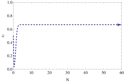
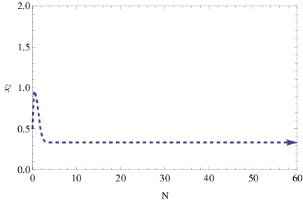
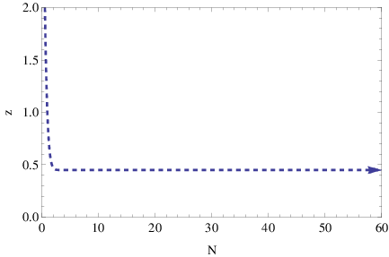
From Fig. 1 it is obvious that a stable fixed point is reached for quite small values of the $e$-foldings number, and we can also demonstrate that indeed this is the case. In Table 1 we present the values of the variables $x_{1}$, $x_{2}$ and $z$ for various values of the $e$-foldings number.

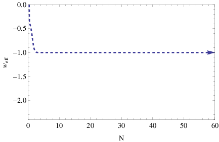
As it can be seen, the fixed point of the dynamical system is $\phi^{*}=(x_{1},x_{2},z)=(0.666667,0.333333,0.449231)$, so let us now investigate the nature of the fixed point. This can be easily done by evaluating the total EoS parameter $w_{eff}$ by using Eq. (12), so in Fig. 2, we present the plots of the total EoS parameter $w_{eff}$ as a function of the $e$-foldings number $N$, for $N$ chosen in the ranges $N=[0,60]$. As it can be seen, the total EoS parameter $w_{eff}$ approaches the value $w_{eff}=-1$ after a few $e$-foldings, so the stable fixed point $\phi^{*}=(x_{1},x_{2},z)=(0.666667,0.333333,0.449231)$ we found numerically, is an exact de Sitter fixed point.

We can further show the existence of an asymptotic attractor in the phase space of the dynamical system (11), by presenting several trajectories in the plane $x_{1}-x_{2}$, for various initial conditions. As it can be seen in Fig. 3, there is an asymptotic attractor for several trajectories which correspond to different initial conditions. Also in Fig. 3 we can also see a trajectory threading the fixed point. After a closer analysis it can be shown that this trajectory drives the system to infinity, so there are initial conditions which may lead to singularities, however these belong to negative initial conditions, so we disregard these trajectories.

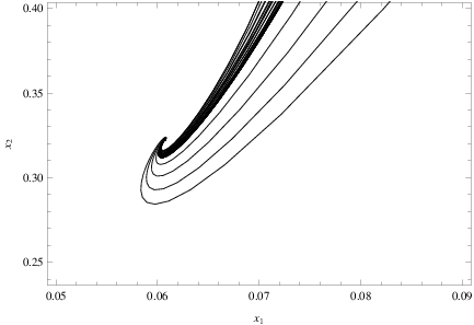
In conclusion, we demonstrated that the classical coupled dark energy-dark matter system with the generalized logarithmic dark energy EoS (8) has stable de Sitter attractors. It is noteworthy that the logarithmic term contributes significantly to the stabilization of the final attractor, and also we need to note that the term $\sim B\rho_{d}^{2}$ must be set equal to zero, since it completely destabilizes the phase space. In the next section we shall investigate whether the LQC effects can modify or alter the phase space structure of the classical phase space. As we will demonstrate, the effects of the LQC theoretical framework are significant since the parameter space for which the existence of stable de Sitter attractors is guaranteed, is enlarged.

Before closing, we shall further discuss the stability issue of the attractors we found in this section, and also we specify the significance of the logarithmic and other terms in the generalized EoS (8). As it is found by our numerical analysis, the appearance of the logarithmic term is crucial for the stability of the final attractors. This feature was also found in Ref. Odintsov:2018obx, however in Ref. Odintsov:2018obx, only the logarithmic term was included, and the resulting de Sitter attractors were quintessential, not de Sitter. In the present case with generalized EoS, the final attractors are stable, an effect guaranteed by the logarithmic term, and most importantly, the attractors are de Sitter, which is the effect of the third and fourth term of the generalized EoS (8). Finally it is crucial to note that the attractors occur only when $B=0$, so the second term of the generalized EoS (8), destabilizes the final attractors.

In this section we shall repeat the study we performed in the previous section, by incorporating LQC effects in the theory. As we shall see, the LQC effects have a significant contribution to the resulting picture, since the existence of stable de Sitter attractors is ensured for a wider range of free variables, and also we have de Sitter attractors even in the case that $B\neq 0$, a feature certainly absent in the classical theoretical framework. The essential features of LQC can be found in various articles, see for example Refs. LQC1; LQC3; LQC4; LQC5; Salo:2016dsr; Xiong:2007cn; Amoros:2014tha; Cai:2014zga; deHaro:2014kxa; Kleidis:2018plu; Kleidis:2017ftt, so we start of with the LQC Friedmann equation which for the flat FRW metric of Eq. (1) becomes,

$$H^{2}=\frac{\kappa^{2}\rho_{tot}}{3}\left(1-\frac{\rho_{tot}}{\rho_{c}}\right)\,,$$

(13)

where $\rho_{tot}$ is the total energy density $\rho_{tot}=\rho_{d}+\rho_{m}$. The dark energy and dark matter continuity equations are still given by (5) and the interaction term is given by (6). By combining Eqs. (13) and (5), we obtain,

$$\dot{H}=-\frac{\kappa^{2}}{2}\left(\rho_{m}+\rho_{d}+p_{tot}\right)\left(1-2\frac{\rho_{m}+\rho_{d}}{\rho_{c}}\right)\,,$$

(14)

with $p_{tot}$ being the total pressure which is again in this case equal to $p_{tot}=p_{d}$. In addition, the dark energy EoS parameter $w_{eff}$ is assumed to be in this case,

$$p_{d}=A\rho_{d}\ln\left(\frac{\kappa^{2}\rho_{d}}{3H^{2}}\right)-\frac{B\rho_{d}^{2}}{\rho_{c}}-\frac{\Lambda\rho_{c}^{2}}{\rho_{d}}-\rho_{d}-\rho_{d}w_{d}\,,$$

(15)

where $B$, $w_{d}$ and $A$ are dimensionless parameters. In order to construct an autonomous dynamical system in the LQC case, we choose the variables of the dynamical system as follows,

$$x_{1}=\frac{\kappa^{2}\rho_{d}}{3H^{2}},\,\,\,x_{2}=\frac{\kappa^{2}\rho_{m}}{3H^{2}},\,\,\,z=\frac{H^{2}}{\kappa^{2}\rho_{c}}\,.$$

(16)

Accordingly, in terms of the variables (16), the total EoS parameter $w_{eff}$ is written as follows,

$$w_{eff}=-\frac{-9Ax_{1}^{2}z^{2}\ln(x_{1})+27Bx_{1}^{3}z^{3}+\Lambda+9(w_{d}+1)x_{1}^{2}z^{2}}{9x_{1}z^{2}(x_{1}+x_{2})}\,.$$

(17)

Thus by using Eqs. (13), (14), (5), and (16), after some extensive algebraic manipulations, the autonomous dynamical system in the LQC case reads,

		$\displaystyle\frac{\mathrm{d}x_{1}}{\mathrm{d}N}=-18Ax_{1}^{3}z\log(x_{1})-18Ax_{1}^{2}x_{2}z\log(x_{1})+3Ax_{1}^{2}\log(x_{1})-3Ax_{1}\log(x_{1})+54Bx_{1}^{4}z^{2}$		(18)
		$\displaystyle+54Bx_{1}^{3}x_{2}z^{2}-9Bx_{1}^{3}z+9Bx_{1}^{2}z-c_{1}x_{2}-c_{2}x_{1}+18w_{d}x_{1}^{3}z+18w_{d}x_{1}^{2}x_{2}z$
		$\displaystyle-3w_{d}x_{1}^{2}+3w_{d}x_{1}-18x_{1}^{2}x_{2}z-18x_{1}x_{2}^{2}z+3x_{1}x_{2}+\frac{\Lambda}{3x_{1}z^{2}}+\frac{2\Lambda x_{1}}{z}+\frac{2\Lambda x_{2}}{z}-\frac{\Lambda}{3z^{2}}\,,$
		$\displaystyle\frac{\mathrm{d}x_{2}}{\mathrm{d}N}=-18Ax_{1}^{2}x_{2}z\log(x_{1})-18Ax_{1}x_{2}^{2}z\log(x_{1})+3Ax_{1}x_{2}\log(x_{1})$
		$\displaystyle+54Bx_{1}^{3}x_{2}z^{2}+54Bx_{1}^{2}x_{2}^{2}z^{2}-9Bx_{1}^{2}x_{2}z+c_{1}x_{2}+c_{2}x_{1}$
		$\displaystyle+18w_{d}x_{1}^{2}x_{2}z+18w_{d}x_{1}x_{2}^{2}z-3w_{d}x_{1}x_{2}+\frac{2\Lambda x_{2}^{2}}{x_{1}z}-18x_{1}x_{2}^{2}z-\frac{\Lambda x_{2}}{3x_{1}z^{2}}-18x_{2}^{3}z+3x_{2}^{2}+\frac{2\Lambda x_{2}}{z}-3x_{2}\,,$
		$\displaystyle\frac{\mathrm{d}z}{\mathrm{d}N}=18Ax_{1}^{2}z^{2}\log(x_{1})+18Ax_{1}x_{2}z^{2}\log(x_{1})-3Ax_{1}z\log(x_{1})-54Bx_{1}^{3}z^{3}-54Bx_{1}^{2}x_{2}z^{3}+9Bx_{1}^{2}z^{2}$
		$\displaystyle-2\Lambda-18w_{d}x_{1}^{2}z^{2}-18w_{d}x_{1}x_{2}z^{2}+3w_{d}x_{1}z-\frac{2\Lambda x_{2}}{x_{1}}+18x_{1}x_{2}z^{2}+\frac{\Lambda}{3x_{1}z}+18x_{2}^{2}z^{2}-3x_{2}z\,.$

The dynamical system (18) is an autonomous dynamical system, however it is quite complicated to study it analytically, so we will rely to numerical analysis again. After a thorough investigation of the free parameters space, the resulting picture is more rich in comparison to the classical case, since the existence of a stable de Sitter attractor occurs for a wider range of the free parameters values. For example, we found the following class of parameter values which guaranteed the existence of a stable de Sitter attractor,

		$\displaystyle A>0,\,\,\,c_{1}>0,\,\,\,c_{2}>0,\,\,\,w_{d}<0,\,\,\,\Lambda<0,\,\,\,B=0\,,$		(19)
		$\displaystyle A<0,\,\,\,c_{1}<0,\,\,\,c_{2}<0,\,\,\,w_{d}>0,\,\,\,\Lambda>0,\,\,\,B<0\,,$
		$\displaystyle A>0,\,\,\,c_{1}>0,\,\,\,c_{2}>0,\,\,\,w_{d}<0,\,\,\,\Lambda<0,\,\,\,B<0\,,$
		$\displaystyle A>0,\,\,\,c_{1}>0,\,\,\,c_{2}>0,\,\,\,w_{d}<0,\,\,\,\Lambda=0,\,\,\,B=0\,,$

and there are more combinations not listed here, that yield similar phenomenological behavior. From Eq. (19) we can readily spot two major differences of the LQC case, in comparison with the classical picture, firstly, the stable de Sitter final attractor occurs for positive values of the parameter $A$ and secondly, the parameter $B$ can also take non-zero values. These cases were absent in the classical approach, since positive values of the parameter $A$ were not allowed, and also non-zero values of the parameter $B$, utterly destabilized the phase space. Let us study the phase space structure for one of the above cases, so let us choose for example the following set of values for the free variables $(A,B,c_{1},c_{2},w_{d},\Lambda)=(1,-1,1,1,-\frac{1}{3},-1)$, and in Fig. 4 we plot the behavior of the variables $x_{1}$, $x_{2}$ and $z$ for the first 60 $e$-foldings.

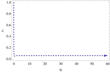
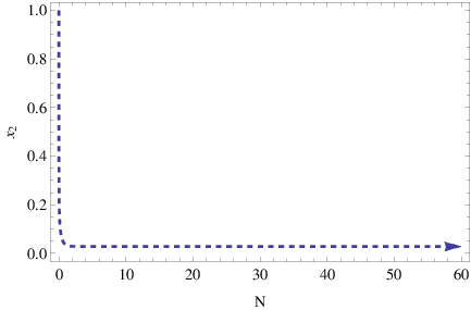
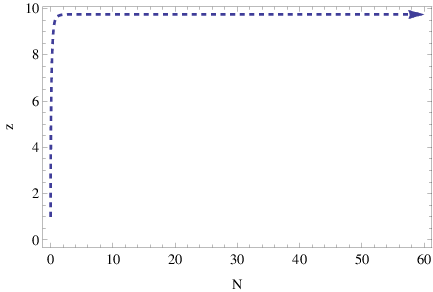
From the plots of Fig. 4 it is obvious that a stable fixed point is reached quite fast. We can find numerically which is the fixed point, so in Table 2, we present the values of the variables $x_{1}$, $x_{2}$ and $z$ for various values of the $e$-foldings number.

As it can be seen in Table 2, the fixed point of the dynamical system in the LQC case is $\phi^{*}=(x_{1},x_{2},z)=(0.057149,0.0285745,9.74264)$. As in the classical case, the fixed point is a de Sitter fixed point, as it can be seen in Fig. 5, where we present the functional dependence of the total EoS parameter $w_{eff}$ as a function of the $e$-foldings number $N$, for $N$ chosen in the range $N=[0,60]$. It is obvious from Fig. 5 that the total EoS parameter approaches quite quickly the de Sitter value $w_{eff}=-1$. In effect, the fixed point $\phi^{*}=(x_{1},x_{2},z)=(0.057149,0.0285745,9.74264)$ is an exact stable de Sitter fixed point.

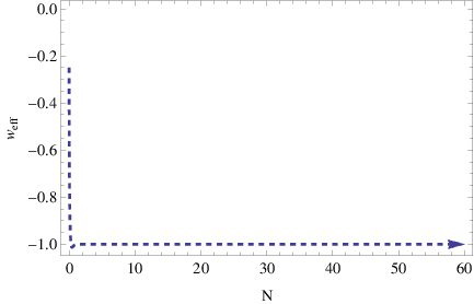
So the LQC case of the coupled dark energy-dark matter cosmological system has more phenomenological interest in comparison to the classical one, due to the fact that, the terms that caused instabilities in the classical case, are allowed in the LQC case, and also these can provide a qualitatively interesting phenomenology. Also the free parameters allowed values are significantly more in number in comparison to the classical case, so in the LQC case, a qualitatively more interesting phenomenology is obtained.

In this paper we investigated the phase space of a coupled dark energy-dark matter cosmological system, in which the dark energy EoS has a generalized functional form containing logarithmic, quadratic and Chaplygin gas-like terms of the energy density. We used two theoretical contexts, namely that of classical Einstein-Hilbert gravity and that of LQC, and we focused the phase space study on the existence and stability of stable de Sitter attractors. After appropriately choosing the variables, we constructed an autonomous dynamical system for both the classical and the LQC cases. With regard to the classical case, we demonstrated that there exist values of the free parameters for which de Sitter attractors exist. By using a numerical approach, we showed that the fixed points are actually stable de Sitter attractors. With regard to the LQC case, we also demonstrated that stable de Sitter attractors exist, and these occur for a wider range of the free parameters values. Actually, for the classical case, we showed that when quadratic terms of the form $\sim\rho_{d}^{2}$ exist in the dark energy EoS, the corresponding dynamical system does not have stable de Sitter attractors, and actually the phase space trajectories become strongly destabilized. In the LQC case, this phenomenon does not occur, since the terms proportional to $\sim\rho_{d}^{2}$ are allowed and can lead to stable de Sitter attractors. Also in the classical case, the logarithmic term must have a negative sign in order to have stable de Sitter attractors, but in the LQC case this constraint is raised and both negative and positive signs of the logarithmic term can lead to stable de Sitter attractors.

An important issue we did not address is the occurrence of finite-time singularities in the cosmological system of the coupled dark energy-dark matter which we studied. Due to the presence of the logarithmic and Chaplygin gas terms, the analytical method of the dominant balances used in Refs. Odintsov:2018uaw; Odintsov:2018awm cannot be used in this case due to the fact that the dynamical system is not polynomial. Therefore, one should try to address this issue numerically, but without any analytical results, it is difficult to extract any useful information from the resulting picture. So approximations are needed near the finite-time singularities, but this task is highly non-trivial and difficult to solve for the coupled fluids system. Perhaps the best strategy is to study the single logarithmic dark energy fluid case, and examine the behavior near the singularities. Another issue which we did not address is to further modify the equation of state and use terms of the form $\sim\rho_{d}^{n}$, with $n$ some positive rational number. This could have some effect on the classical Einstein-Hilbert system, so we hope to address this issue in a future work.

References

- (1) A. G. Riess et al. [Supernova Search Team], Astron. J. 116 (1998) 1009 doi:10.1086/300499 [astro-ph/9805201].
- (2) R. R. Caldwell, M. Kamionkowski and N. N. Weinberg, Phys. Rev. Lett. 91 (2003) 071301 [astro-ph/0302506].
- (3) S. Tulin and H. B. Yu, Phys. Rept. 730 (2018) 1 doi:10.1016/j.physrep.2017.11.004 [arXiv:1705.02358 [hep-ph]].
- (4) L. Berezhiani and J. Khoury, Phys. Rev. D 92 (2015) 103510 doi:10.1103/PhysRevD.92.103510 [arXiv:1507.01019 [astro-ph.CO]].
- (5) L. Berezhiani and J. Khoury, Phys. Lett. B 753 (2016) 639 doi:10.1016/j.physletb.2015.12.054 [arXiv:1506.07877 [astro-ph.CO]].
- (6) A. Hodson, H. Zhao, J. Khoury and B. Famaey, Astron. Astrophys. 607 (2017) A108 doi:10.1051/0004-6361/201630069 [arXiv:1611.05876 [astro-ph.CO]].
- (7) L. Berezhiani, B. Famaey and J. Khoury, arXiv:1711.05748 [astro-ph.CO].
- (8) V. K. Oikonomou, J. D. Vergados and C. C. Moustakidis, Nucl. Phys. B 773 (2007) 19 doi:10.1016/j.nuclphysb.2007.03.014 [hep-ph/0612293].
- (9) S. Nojiri, S. D. Odintsov and V. K. Oikonomou, Phys. Rept. 692 (2017) 1 doi:10.1016/j.physrep.2017.06.001 [arXiv:1705.11098 [gr-qc]].
- (10) S. Nojiri, S.D. Odintsov, Phys. Rept. 505, 59 (2011);
- (11) S. Nojiri, S.D. Odintsov, eConf C0602061, 06 (2006) [Int. J. Geom. Meth. Mod. Phys. 4, 115 (2007)].
- (12)
S. Capozziello, M. De Laurentis,
Phys. Rept. 509, 167 (2011);
V. Faraoni and S. Capozziello, Fundam. Theor. Phys. 170 (2010). doi:10.1007/978-94-007-0165-6 - (13) A. de la Cruz-Dombriz and D. Saez-Gomez, Entropy 14 (2012) 1717 doi:10.3390/e14091717 [arXiv:1207.2663 [gr-qc]].
- (14) G. J. Olmo, Int. J. Mod. Phys. D 20 (2011) 413 doi:10.1142/S0218271811018925 [arXiv:1101.3864 [gr-qc]].
- (15) S. Nojiri and S. D. Odintsov, Phys. Rev. D 68 (2003) 123512 doi:10.1103/PhysRevD.68.123512 [hep-th/0307288].
- (16) P. Gondolo and K. Freese, Phys. Rev. D 68 (2003) 063509 doi:10.1103/PhysRevD.68.063509 [hep-ph/0209322].
- (17) G. R. Farrar and P. J. E. Peebles, Astrophys. J. 604 (2004) 1 doi:10.1086/381728 [astro-ph/0307316].
- (18) R. G. Cai and A. Wang, JCAP 0503 (2005) 002 doi:10.1088/1475-7516/2005/03/002 [hep-th/0411025].
- (19) Z. K. Guo, R. G. Cai and Y. Z. Zhang, JCAP 0505 (2005) 002 doi:10.1088/1475-7516/2005/05/002 [astro-ph/0412624].
- (20) B. Wang, J. Zang, C. Y. Lin, E. Abdalla and S. Micheletti, Nucl. Phys. B 778 (2007) 69 doi:10.1016/j.nuclphysb.2007.04.037 [astro-ph/0607126].
- (21) O. Bertolami, F. Gil Pedro and M. Le Delliou, Phys. Lett. B 654 (2007) 165 doi:10.1016/j.physletb.2007.08.046 [astro-ph/0703462 [ASTRO-PH]].
- (22) J. H. He and B. Wang, JCAP 0806 (2008) 010 doi:10.1088/1475-7516/2008/06/010 [arXiv:0801.4233 [astro-ph]].
- (23) J. Valiviita, E. Majerotto and R. Maartens, JCAP 0807 (2008) 020 doi:10.1088/1475-7516/2008/07/020 [arXiv:0804.0232 [astro-ph]].
- (24) B. M. Jackson, A. Taylor and A. Berera, Phys. Rev. D 79 (2009) 043526 doi:10.1103/PhysRevD.79.043526 [arXiv:0901.3272 [astro-ph.CO]].
- (25) M. Jamil, E. N. Saridakis and M. R. Setare, Phys. Rev. D 81 (2010) 023007 doi:10.1103/PhysRevD.81.023007 [arXiv:0910.0822 [hep-th]].
- (26) J. H. He, B. Wang and E. Abdalla, Phys. Rev. D 83 (2011) 063515 doi:10.1103/PhysRevD.83.063515 [arXiv:1012.3904 [astro-ph.CO]].
- (27) Y. L. Bolotin, A. Kostenko, O. A. Lemets and D. A. Yerokhin, Int. J. Mod. Phys. D 24 (2014) no.03, 1530007 doi:10.1142/S0218271815300074 [arXiv:1310.0085 [astro-ph.CO]].
- (28) A. A. Costa, X. D. Xu, B. Wang, E. G. M. Ferreira and E. Abdalla, Phys. Rev. D 89 (2014) no.10, 103531 doi:10.1103/PhysRevD.89.103531 [arXiv:1311.7380 [astro-ph.CO]].
- (29) C. G. Boehmer, G. Caldera-Cabral, R. Lazkoz and R. Maartens, Phys. Rev. D 78 (2008) 023505 doi:10.1103/PhysRevD.78.023505 [arXiv:0801.1565 [gr-qc]].
- (30) S. Li and Y. Ma, Eur. Phys. J. C 68 (2010) 227 doi:10.1140/epjc/s10052-010-1338-y [arXiv:1004.4350 [astro-ph.CO]].
- (31) W. Yang, S. Pan and J. D. Barrow, arXiv:1706.04953 [astro-ph.CO].
- (32) K. Bamba, S. Capozziello, S. Nojiri and S. D. Odintsov, Astrophys. Space Sci. 342 (2012) 155, [arXiv:1205.3421 [gr-qc]].
- (33) J. D. Barrow and J. P. Mimoso, Phys. Rev. D 50 (1994) 3746. doi:10.1103/PhysRevD.50.3746
- (34) C. G. Tsagas and J. D. Barrow, Class. Quant. Grav. 15 (1998) 3523 doi:10.1088/0264-9381/15/11/016 [gr-qc/9803032].
- (35) W. S. Hipolito-Ricaldi, H. E. S. Velten and W. Zimdahl, JCAP 0906 (2009) 016 doi:10.1088/1475-7516/2009/06/016 [arXiv:0902.4710 [astro-ph.CO]].
- (36) V. Gorini, A. Kamenshchik, U. Moschella, V. Pasquier and A. Starobinsky, Phys. Rev. D 72 (2005) 103518 doi:10.1103/PhysRevD.72.103518 [astro-ph/0504576].
- (37) G. M. Kremer, Phys. Rev. D 68 (2003) 123507 doi:10.1103/PhysRevD.68.123507 [gr-qc/0309111].
- (38) I. Brevik, V. V. Obukhov and A. V. Timoshkin, Int. J. Geom. Meth. Mod. Phys. 15 (2018) no.09, 1850150 doi:10.1142/S0219887818501505 [arXiv:1805.01258 [gr-qc]].
- (39) D. Carturan and F. Finelli, Phys. Rev. D 68 (2003) 103501 doi:10.1103/PhysRevD.68.103501 [astro-ph/0211626].
- (40) T. Buchert, Gen. Rel. Grav. 33 (2001) 1381 doi:10.1023/A:1012061725841 [gr-qc/0102049].
- (41) J. c. Hwang and H. Noh, Class. Quant. Grav. 19 (2002) 527 doi:10.1088/0264-9381/19/3/308 [astro-ph/0103244].
- (42) N. Cruz, S. Lepe and F. Pena, Phys. Lett. B 699 (2011) 135. doi:10.1016/j.physletb.2011.03.049
- (43) V. K. Oikonomou, Int. J. Mod. Phys. D 26 (2017) no.10, 1750110 doi:10.1142/S0218271817501103 [arXiv:1703.09009 [gr-qc]].
- (44) I. Brevik, E. Elizalde, S. D. Odintsov and A. V. Timoshkin, Int. J. Geom. Meth. Mod. Phys. 14 (2017) no.12, 1750185 doi:10.1142/S0219887817501857 [arXiv:1708.06244 [gr-qc]].
- (45) I. Brevik, O. Gron, J. de Haro, S. D. Odintsov and E. N. Saridakis, Int. J. Mod. Phys. D 26 (2017) no.14, 1730024 doi:10.1142/S0218271817300245 [arXiv:1706.02543 [gr-qc]].
- (46) S. Nojiri and S. D. Odintsov, Phys. Rev. D 72 (2005) 023003 doi:10.1103/PhysRevD.72.023003 [hep-th/0505215].
- (47) S. Capozziello, S. Nojiri, S. D. Odintsov and A. Troisi, Phys. Lett. B 639 (2006) 135 doi:10.1016/j.physletb.2006.06.034 [astro-ph/0604431].
- (48) S. Nojiri and S. D. Odintsov, Phys. Lett. B 639 (2006) 144 doi:10.1016/j.physletb.2006.06.065 [hep-th/0606025].
- (49) E. Elizalde and D. Saez-Gomez, Phys. Rev. D 80 (2009) 044030 doi:10.1103/PhysRevD.80.044030 [arXiv:0903.2732 [hep-th]].
- (50) E. Elizalde and M. Khurshudyan, arXiv:1711.01143 [gr-qc].
- (51) I. Brevik and A. V. Timoshkin, Int. J. Geom. Meth. Mod. Phys. 14 (2017) no.04, 1750061 doi:10.1142/S021988781750061X [arXiv:1612.06689 [gr-qc]].
- (52) A. B. Balakin and V. V. Bochkarev, Phys. Rev. D 87 (2013) no.2, 024006 doi:10.1103/PhysRevD.87.024006 [arXiv:1212.4094 [gr-qc]].
- (53) W. Zimdahl and A. B. Balakin, Class. Quant. Grav. 15 (1998) 3259 doi:10.1088/0264-9381/15/10/026 [gr-qc/9807078].
- (54) M. Kunz, Phys. Rev. D 80 (2009) 123001 doi:10.1103/PhysRevD.80.123001 [astro-ph/0702615].
- (55) S. D. Odintsov, V. K. Oikonomou, A. V. Timoshkin, E. N. Saridakis and R. Myrzakulov, arXiv:1810.01276 [gr-qc].
- (56) V. M. C. Ferreira and P. P. Avelino, Phys. Lett. B 770 (2017) 213 doi:10.1016/j.physletb.2017.03.075 [arXiv:1611.08403 [astro-ph.CO]].
- (57) H. Anton, P.C. Schmidt, Intermetallics. 5 (1997) 449.
- (58) B. Mayer et. al, Intermetallics. 11 (2003) 23.
- (59) A. L. Ivanovskii, Prog. Mat. Scie. 57 (2012) 1.
- (60) S. D. Odintsov and V. K. Oikonomou, Phys. Rev. D 98 (2018) no.2, 024013 doi:10.1103/PhysRevD.98.024013 [arXiv:1806.07295 [gr-qc]].
- (61) S. D. Odintsov and V. K. Oikonomou, Phys. Rev. D 97 (2018) no.12, 124042 doi:10.1103/PhysRevD.97.124042 [arXiv:1806.01588 [gr-qc]].
- (62) C. G. Boehmer and N. Chan, doi:10.1142/9781786341044.0004 arXiv:1409.5585 [gr-qc].
- (63) C. G. Boehmer, T. Harko and S. V. Sabau, Adv. Theor. Math. Phys. 16 (2012) no.4, 1145 doi:10.4310/ATMP.2012.v16.n4.a2 [arXiv:1010.5464 [math-ph]].
- (64) N. Goheer, J. A. Leach and P. K. S. Dunsby, Class. Quant. Grav. 24 (2007) 5689 doi:10.1088/0264-9381/24/22/026 [arXiv:0710.0814 [gr-qc]].
- (65) G. Leon and E. N. Saridakis, JCAP 1504 (2015) no.04, 031 doi:10.1088/1475-7516/2015/04/031 [arXiv:1501.00488 [gr-qc]].
- (66) J. Q. Guo and A. V. Frolov, Phys. Rev. D 88 (2013) no.12, 124036 doi:10.1103/PhysRevD.88.124036 [arXiv:1305.7290 [astro-ph.CO]].
- (67) G. Leon and E. N. Saridakis, Class. Quant. Grav. 28 (2011) 065008 doi:10.1088/0264-9381/28/6/065008 [arXiv:1007.3956 [gr-qc]].
- (68) J. C. C. de Souza and V. Faraoni, Class. Quant. Grav. 24 (2007) 3637 doi:10.1088/0264-9381/24/14/006 [arXiv:0706.1223 [gr-qc]].
- (69) A. Giacomini, S. Jamal, G. Leon, A. Paliathanasis and J. Saavedra, Phys. Rev. D 95 (2017) no.12, 124060 doi:10.1103/PhysRevD.95.124060 [arXiv:1703.05860 [gr-qc]].
- (70) G. Kofinas, G. Leon and E. N. Saridakis, Class. Quant. Grav. 31 (2014) 175011 doi:10.1088/0264-9381/31/17/175011 [arXiv:1404.7100 [gr-qc]].
- (71) G. Leon and E. N. Saridakis, JCAP 1303 (2013) 025 doi:10.1088/1475-7516/2013/03/025 [arXiv:1211.3088 [astro-ph.CO]].
- (72) T. Gonzalez, G. Leon and I. Quiros, Class. Quant. Grav. 23 (2006) 3165 doi:10.1088/0264-9381/23/9/025 [astro-ph/0702227].
- (73) A. Alho, S. Carloni and C. Uggla, JCAP 1608 (2016) no.08, 064 doi:10.1088/1475-7516/2016/08/064 [arXiv:1607.05715 [gr-qc]].
- (74) S. K. Biswas and S. Chakraborty, Int. J. Mod. Phys. D 24 (2015) no.07, 1550046 doi:10.1142/S0218271815500467 [arXiv:1504.02431 [gr-qc]].
- (75) D. Muller, V. C. de Andrade, C. Maia, M. J. Reboucas and A. F. F. Teixeira, Eur. Phys. J. C 75 (2015) no.1, 13 doi:10.1140/epjc/s10052-014-3227-2 [arXiv:1405.0768 [astro-ph.CO]].
- (76) B. Mirza and F. Oboudiat, Int. J. Geom. Meth. Mod. Phys. 13 (2016) no.09, 1650108 doi:10.1142/S0219887816501085 [arXiv:1412.6640 [gr-qc]].
- (77) S. Rippl, H. van Elst, R. K. Tavakol and D. Taylor, Gen. Rel. Grav. 28 (1996) 193 doi:10.1007/BF02105423 [gr-qc/9511010].
- (78) M. M. Ivanov and A. V. Toporensky, Grav. Cosmol. 18 (2012) 43 doi:10.1134/S0202289312010100 [arXiv:1106.5179 [gr-qc]].
- (79) M. Khurshudyan, Int. J. Geom. Meth. Mod. Phys. 14 (2016) no.03, 1750041. doi:10.1142/S0219887817500414
- (80) R. D. Boko, M. J. S. Houndjo and J. Tossa, Int. J. Mod. Phys. D 25 (2016) no.10, 1650098 doi:10.1142/S021827181650098X [arXiv:1605.03404 [gr-qc]].
- (81) S. D. Odintsov, V. K. Oikonomou and P. V. Tretyakov, Phys. Rev. D 96 (2017) no.4, 044022 doi:10.1103/PhysRevD.96.044022 [arXiv:1707.08661 [gr-qc]].
- (82) L. N. Granda and D. F. Jimenez, arXiv:1710.07273 [gr-qc].
- (83) F. F. Bernardi and R. G. Landim, Eur. Phys. J. C 77 (2017) no.5, 290 doi:10.1140/epjc/s10052-017-4858-x [arXiv:1607.03506 [gr-qc]].
- (84) R. C. G. Landim, Eur. Phys. J. C 76 (2016) no.1, 31 doi:10.1140/epjc/s10052-016-3894-2 [arXiv:1507.00902 [gr-qc]].
- (85) R. C. G. Landim, Eur. Phys. J. C 76 (2016) no.9, 480 doi:10.1140/epjc/s10052-016-4328-x [arXiv:1605.03550 [hep-th]].
- (86) P. Bari, K. Bhattacharya and S. Chakraborty, arXiv:1805.06673 [gr-qc].
- (87) S. Chakraborty, arXiv:1805.03237 [gr-qc].
- (88) M. G. Ganiou, P. H. Logbo, M. J. S. Houndjo and J. Tossa, arXiv:1805.00332 [gr-qc].
- (89) P. Shah, G. C. Samanta and S. Capozziello, arXiv:1803.09247 [gr-qc].
- (90) V. K. Oikonomou, Int. J. Mod. Phys. D 27 (2018) no.05, 1850059 doi:10.1142/S0218271818500591 [arXiv:1711.03389 [gr-qc]].
- (91) S. D. Odintsov and V. K. Oikonomou, Phys. Rev. D 96 (2017) no.10, 104049 doi:10.1103/PhysRevD.96.104049 [arXiv:1711.02230 [gr-qc]].
- (92) J. Dutta, W. Khyllep, E. N. Saridakis, N. Tamanini and S. Vagnozzi, JCAP 1802 (2018) 041 doi:10.1088/1475-7516/2018/02/041 [arXiv:1711.07290 [gr-qc]].
- (93) S. D. Odintsov and V. K. Oikonomou, Phys. Rev. D 93 (2016) no.2, 023517 doi:10.1103/PhysRevD.93.023517 [arXiv:1511.04559 [gr-qc]].
- (94) K. Kleidis and V. K. Oikonomou, arXiv:1808.04674 [gr-qc].
- (95) V. K. Oikonomou and N. Chatzarakis, arXiv:1905.01904 [gr-qc].
- (96) V. K. Oikonomou, Phys. Rev. D 99 (2019) no.10, 104042 doi:10.1103/PhysRevD.99.104042 [arXiv:1905.00826 [gr-qc]].
- (97) A. Ashtekar and P. Singh, Class. Quant. Grav. 28 (2011) 213001 [arXiv:1108.0893 [gr-qc]]
- (98) A. Ashtekar, T. Pawlowski and P. Singh, Phys. Rev. Lett. 96 (2006) 141301 [gr-qc/0602086].
- (99) A. Ashtekar, T. Pawlowski and P. Singh, Phys. Rev. D 73 (2006) 124038 [gr-qc/0604013].
- (100) A. Ashtekar, T. Pawlowski and P. Singh, Phys. Rev. D 74 (2006) 084003 [gr-qc/0607039].
- (101) L. Areste Salo, J. Amoros and J. de Haro, Class. Quant. Grav. 34 (2017) no.23, 235001 doi:10.1088/1361-6382/aa9311 [arXiv:1612.05480 [gr-qc]].
- (102) H. H. Xiong, T. Qiu, Y. F. Cai and X. Zhang, Mod. Phys. Lett. A 24 (2009) 1237 doi:10.1142/S0217732309030667 [arXiv:0711.4469 [hep-th]].
- (103) J. Amoros, J. de Haro and S. D. Odintsov, Phys. Rev. D 89 (2014) no.10, 104010 doi:10.1103/PhysRevD.89.104010 [arXiv:1402.3071 [gr-qc]].
- (104) Y. F. Cai and E. Wilson-Ewing, JCAP 1403 (2014) 026 doi:10.1088/1475-7516/2014/03/026 [arXiv:1402.3009 [gr-qc]].
- (105) J. de Haro and J. Amoros, JCAP 1408 (2014) 025 doi:10.1088/1475-7516/2014/08/025 [arXiv:1403.6396 [gr-qc]].
- (106) K. Kleidis and V. K. Oikonomou, Int. J. Geom. Meth. Mod. Phys. 15 (2018) no.05, 1850071 doi:10.1142/S0219887818500718 [arXiv:1801.02578 [gr-qc]].
- (107) K. Kleidis and V. K. Oikonomou, Int. J. Geom. Meth. Mod. Phys. 15 (2017) no.04, 1850064 doi:10.1142/S0219887818500640 [arXiv:1711.09270 [gr-qc]].
- (108) G. Caldera-Cabral, R. Maartens and L. A. Urena-Lopez, Phys. Rev. D 79 (2009) 063518 doi:10.1103/PhysRevD.79.063518 [arXiv:0812.1827 [gr-qc]].
- (109) D. Pavon and W. Zimdahl, Phys. Lett. B 628 (2005) 206 doi:10.1016/j.physletb.2005.08.134 [gr-qc/0505020].
- (110) M. Quartin, M. O. Calvao, S. E. Joras, R. R. R. Reis and I. Waga, JCAP 0805 (2008) 007 doi:10.1088/1475-7516/2008/05/007 [arXiv:0802.0546 [astro-ph]].
- (111) H. M. Sadjadi and M. Alimohammadi, Phys. Rev. D 74 (2006) 103007 doi:10.1103/PhysRevD.74.103007 [gr-qc/0610080].
- (112) W. Zimdahl, Int. J. Mod. Phys. D 14 (2005) 2319 doi:10.1142/S0218271805007784 [gr-qc/0505056].
- (113) M. C. Bento, O. Bertolami and A. A. Sen, Phys. Rev. D 66 (2002) 043507 doi:10.1103/PhysRevD.66.043507 [gr-qc/0202064].
- (114) N. Bilic, G. B. Tupper and R. D. Viollier, Phys. Lett. B 535 (2002) 17 doi:10.1016/S0370-2693(02)01716-1 [astro-ph/0111325].
- (115) M. Khurshudyan, Int. J. Geom. Meth. Mod. Phys. 15 (2018) no.09, 1850155. doi:10.1142/S0219887818501554