Fair Kernel Regression via Fair Feature Embedding in Kernel Space

To facilitate discussions in related work, we introduce some notations here. We describe an instance using a triple $(x,s,y)$, where $x$ is a feature vector, $s$ is a protected demographic (e.g. gender, race) and $y$ is label. Assume $s$ is contained in $x$.

Similar to prior studies, we assume $s$ is binary. Let there be $n$ instances in the training set, among which $n_{u}$ belong to the unprotected group (s = 0) and $n_{p}$ belong to the protected group (s = 1). Without loss of generality, we assume the instances are ordered such that the first $n_{u}$ ones $x_{1},\ldots,x_{n_{u}}$ are unprotected and the rest $x_{n_{u}+1},\ldots,x_{n}$ are protected.

For kernel methods, let $\phi(\cdot)$ be the feature mapping function, and $f$ be a prediction model mapping from $\phi(x)$ to $y$.

Perez-Suay et al [13] propose a fair kernel regression method, which directly extends the linear fair learning method [9] to kernel space. Specifically, it minimizes prediction loss while additionally penalizing the correlation between model prediction and demographic feature in the kernel space as:

$\displaystyle\begin{split}&\min_{f}\sum_{i=1}^{n}[f(\phi(x_{i}))-y_{i}]^{2}+\mu\sum_{i=1}^{n}(\bar{f}(x_{i})\cdot\bar{s}_{i})+\lambda\Omega(f),\end{split}$

(1)

where the second term measures predictive bias as the correlation between model prediction and the demographic feature, and $\bar{f}(x)$ and $\bar{s}$ are centered variables; the last term measures model complexity; $\mu$ and $\lambda$ are hyper-parameters. Based on the Representer Theorem that $f$ is a linear combination of $\phi(x_{i})$’s, task (1) admits an analytic solution for the linear coefficients.

Perez et al’s method adopts the regularization approach in fair learning, which penalizes predictive bias during learning (e.g., [8, 9]). In this paper, we adopt another popular approach which first constructs a fair feature space and then builds a standard model in it (e.g., [6, 7, 12]). In experiments, we show our method can achieve higher prediction fairness.

An effective approach to learn fair models is to first construct a fair feature space and then learn a standard model in it (e.g., [6, 7]). A fair feature space is one where feature distributions of different demographic groups are similar, e.g., different groups have similar CDF’s of the new features [7], or the statistical dependence between the new features and the demographic feature is low [6].

In this paper, we develop a new fair kernel regression based on the idea of fair feature learning. Unlike previous studies, we measure feature similarity using mean discrepancy [16]. MD measures distance between distributions and is widely used in machine learning [17, 18, 19]. Let $x_{1},\ldots,x_{n}$ and $z_{1},\ldots,z_{m}$ be two sets generated from distributions $P_{x}$ and $P_{z}$ respectively. MD estimates the distance between $P_{x}$ and $P_{z}$ as

$$MD(P_{x},P_{z})=\left|\left|\frac{1}{n}\sum_{i=1}^{n}\phi(x_{i})-\frac{1}{m}\sum_{j=1}^{m}\phi(z_{j})\right|\right|^{2}.$$

(2)

A technical challenge is that previous fair feature learning approaches assume the feature space is explicit and then modify it to obtain a fairer space. In kernel methods, however, the feature space of $\phi(x)$ is implicit. To tackle this issue, we propose to construct an explicit fair feature space for $\phi(x)$, by learning fair feature embedding functions in the kernel space. This approach is motivated by the literature of feature selection in kernel methods (e.g., [20, 15]).

Feature selection is a common practice for improving the robustness and interpretability of machine learning models [21]. However, its practice in kernel methods is not easy, since there is not an explicit feature representation in kernel space. Only a few approaches are proposed, e.g. [20, 22, 15].

Our study is motivated by Cao et al [15]. They propose to learn explicit feature representation in the kernel space, by learning feature embedding function $\eta$. They show the optimal function is a linear combination of training instances, and learn such functions by standard methods such as KPCA [23]. After that, instance $\phi(x)$ is mapped onto $\eta$ to obtain an explicit feature representation on which feature selection is performed.

Motivated by Cao et al’s approach, we propose to learn feature embedding functions that are fair, e.g.., different demographic groups have similar distributions in the embedded space. As explained in the previous subsection, similarity is measured by mean discrepancy.

Our goal is to learn an explicit and fair feature representation for $\phi(x)$. To that end, we propose to learn a fair feature embedding function $\eta$, such that in the embedded space, the mean discrepancy between the protected group and unprotected group is minimized:

$$\min_{\eta}\left|\left|\frac{1}{n_{u}}\sum_{i=1}^{n_{u}}\langle\phi(x_{i}),\eta\rangle-\frac{1}{n_{p}}\sum_{i=n_{u}+1}^{n}\langle\phi(x_{i}),\eta\rangle\right|\right|^{2}.$$

(3)

Problem (3) cannot be directly solved since there is no explicit representation of $\phi(x)$. Motivated by Cao et al [15], we assume the optimal $\eta$ is a linear combination of training instances:

$$\eta={\sum}_{i=1}^{n}\alpha_{i}\phi(x_{i}).$$

(4)

To avoid overfitting, we further assume $\eta$ has a unit norm:

$$||\eta||^{2}=1.$$

(5)

Solving (3) under constraints (4) and (5), we have that¹¹ 1 Detailed arguments are in Appendix A.

$$\left(\frac{1}{n_{u}^{2}}K_{u}^{T}K_{u}-\frac{2}{n_{u}n_{p}}K_{u}^{T}\mathbf{1}_{u}\mathbf{1}_{p}^{T}K_{p}+\frac{1}{n_{p}^{2}}K_{p}^{T}K_{p}\right)\alpha=\lambda K\alpha,$$

(6)

where $\alpha=[\alpha_{1},\ldots,\alpha_{n}]^{T}$ is the vector of unknown parameters and $\lambda$ is an eigenvalue; $K$ is a standard $n$-by-$n$ Gram matrix of all instances; $K_{u}$ is $n_{u}$-by-$n$ and $K_{p}$ is $n_{p}$-by-$n$ satisfying

$$K=\begin{bmatrix}K_{u}\\ K_{p}\end{bmatrix}$$

(7)

Formula (6) is a generalized eigenproblem, and $\alpha$ is the least generalized eigenvector. After $\alpha$ is solved, we obtain the first explicit and fair feature of $\phi(x)$ in the kernel space as

$$\langle\phi(x),\eta\rangle={\sum}_{i=1}^{n}\alpha_{i}k(x,x_{i}).$$

(8)

The above analysis gives the first fair feature embedding function $\eta$ in the kernel space. Now we present how to obtain the second $\eta^{\prime}$, and the rest can be derived in similar fashions.

The second optimal embedding $\eta^{\prime}$ is obtained in a similar fashion as $\eta$, with an additional constraint that it should be orthogonal to the previously obtained embeddings:

		$\displaystyle\min_{\eta^{\prime}}\left|\left|\frac{1}{n_{u}}\sum_{i=1}^{n_{u}}\langle\phi(x_{i}),\eta^{\prime}\rangle-\frac{1}{n_{p}}\sum_{i=n_{u}+1}^{n}\langle\phi(x_{i}),\eta^{\prime}\rangle\right|\right|^{2}$		(9)
		$\displaystyle s.t.\ \eta^{\prime}={\sum}_{i=1}^{n}\alpha^{\prime}_{i}\phi(x_{i}),\quad||\eta^{\prime}||^{2}=1,\quad\eta^{T}\eta^{\prime}=0.$

Solving (9) shows that $\alpha^{\prime}=[\alpha_{1}^{\prime},\ldots,\alpha_{n}^{\prime}]^{T}$ is the second least generalized eigenvector of the same eigenproblem (6)²² 2 Detailed arguments are in Appendix B. .

By similar arguments, we can show the linear coefficients of $k$ optimal fair embeddings $\eta_{1},\ldots,\eta_{k}$ are the least $k$ generalized eigenvectors of the eigenproblem (6).

After that, we obtain a k-dimensional explicit fair feature representation of $\phi$ in the kernel space, i.e.,

$$\phi_{FS}(x)=[\langle\phi(x),\eta_{1}\rangle,\ldots,\langle\phi(x),\eta_{k}\rangle]^{T}.$$

(10)

Given an explicit fair feature representation $\phi_{FS}(x)$, we learn a standard regression model based on it. Let $x_{1},\ldots,x_{n}$ be $n$ training instances. One can easily verify that

$$\phi_{FS}(x_{i})=[\langle\phi(x_{i}),\eta_{1}\rangle,\ldots,\langle\phi(x_{i}),\eta_{k}\rangle]^{T}=(K_{:i}^{T}A)^{T}$$

(11)

where $K_{:i}$ is the $i^{th}$ column Gram matrix $K$, and $A$ is an $n$-by-$k$ matrix with column j being the linear coefficient vector of $\eta_{j}$ (e.g., the first column is $\alpha$ and the second column is $\alpha^{\prime}$).

Then, one can obtain an $n$-by-$k$ training sample matrix

$$X_{FS}=\begin{bmatrix}(\phi_{FS}(x_{1}))^{T}\\ \vdots\\ (\phi_{FS}(x_{n}))^{T}\end{bmatrix}=\begin{bmatrix}K_{:1}^{T}A\\ \vdots\\ K_{:n}^{T}A\end{bmatrix}=K^{T}A=KA.$$

(12)

Now, we learn a regression model $\beta\in\mathbb{R}^{k}$ on $X_{FS}$ by

$$\min_{\beta}\ ||X_{FS}\cdot\beta-Y||^{2}+\gamma||\beta||^{2},$$

(13)

where $\gamma$ is a regularization coefficient.

For any testing instance $z$, we first compute its explicit fair feature representation

$$\phi_{FS}(z)=[\langle\phi(z),\eta_{1}\rangle,\ldots,\langle\phi(z),\eta_{k}\rangle]^{T},$$

(14)

and then compute its prediction as

$$\hat{y}=\phi_{FS}(z)^{T}\beta.$$

(15)

For classification tasks, one can simply threshold $\hat{y}$.

We experimented on three public data sets, namely, the Credit Default data set³³ 3 https://archive.ics.uci.edu/ml/datasets/default+of+credit+card+clients, the Community Crime data set⁴⁴ 4 http://archive.ics.uci.edu/ml/datasets/communities+and+crime, and the COMPAS data set⁵⁵ 5 https://github.com/propublica/compas-analysis.

The original Credit Default data set contains 30,000 individuals described by 23 attributes. We treated ‘education level’ as the sensitive variable, and binarized it into higher education and lower education as in [12]; ‘default payment’ is treated as the binary label. We removed individuals with missing values and down-sampled the data set from 30,000 to 20,000. Our preprocessed data sets are published at ⁶⁶ 6 https://uwyomachinelearning.github.io/.

The Communities Crime data set contains 1,993 communities described by 101 informative attributes. We treated the ‘fraction of African-American residents’ as the sensitive feature, and binarized it so that a community is ’minority’ if the fraction is above 0.5 and ’majority’ otherwise. Label is the ‘community crime rate’, and we binarized it into high if the rate is above 0.5 and low otherwise.

The COMPAS data set contains 18,317 individuals with 40 features (e.g., name, sex, race). We down-sampled the data set to 16,000 instances and 15 numerical features (e.g. name is removed). Similar to [24], we treated ‘race’ as the sensitive feature and ‘risk of recidivism’ as the binary label.

On each data set, we randomly chose 75% of the instances for training and used the rest for testing. We evaluated each method over 50 random trials and reported its average performance and standard deviation.

We compared the proposed FKR-F²E with the existing fair kernel regression [13], and several other non-kernel methods. For each compared method, we set its hyper-parameters as described in the original paper.

For FKR-F²E, we used polynomial kernel on both Credit and Community Crime data sets and sigmoid kernel on the COMPAS data set. For polynomial kernel, we grid-searched its optimal degree in $\{3,4,5,6\}$ and optimal additive coefficient in $[10^{-3},10^{-2},10^{-1},10^{0},10^{1}]$. For sigmoid kernel, we grid-searched its optimal $c$ among 5 values in the logarithmic range of $[10^{-4},10^{1}]$, and we used the default $\gamma$ in Scikit-Learn [25] (i.e., inverse of feature dimension). For the ridge regression regularization coefficient $\lambda$, we grid-searched an optimal value among 6 values in the logarithmic range $[10^{-3},10^{2}]$.

Finally, an important hyper-parameter is the number of feature embeddings $k$. We experimented with 4 values, namely, $\frac{n}{250}$, $\frac{n}{200}$, $\frac{n}{150}$ and $\frac{n}{100}$. In experiment these values yielded good generalization performance on all data sets.

We evaluated model accuracy using the standard classification error (Error), and evaluated model fairness using a popular measure called statistical disparity (SD) [11], defined as:

$$SD(f,S)=|p(f(x)=1\mid s=1)-p(f(x)=1\mid s=0)|.$$

(16)

Finally, all experiments were run on the Teton Computing Environment at the University of Wyoming’s Advanced Research Computing Center (https://doi.org/10.15786/M2FY47), and our FFE implementation is at https://github.com/aokray/FFE.

Our classification results are summarized in Table I.

Our first observation is that FKR-F²E consistently achieves lower statistical disparity than the existing fair kernel regression method (and other baselines) across the three data sets. This implies that fair feature embedding is an effective approach for learning fair models in kernel space.

We notice the superior fairness of FKR-F²E is not achieved without any cost. In general, it has slightly higher prediction error than the existing fair kernel regression and other baselines. However, we argue the loss of accuracy is small compared with the increase of fairness. For example, on the Credit Default data set, FKR-F²E lowers prediction disparity by at least 75% = (0.0079-0.0021)/0.0079 but only increases prediction error by at most 13% = (0.2277-0.2001)/0.2001. We thus argue this method has a more efficient accuracy-fairness trade-off.

Finally, we see fair kernel methods generally achieve lower statistical disparity than other fair learning methods, suggesting their promisingness for fair machine learning.

In this section, we examined the performance of FKR-F²E on the Communities Crime data set under different configurations.

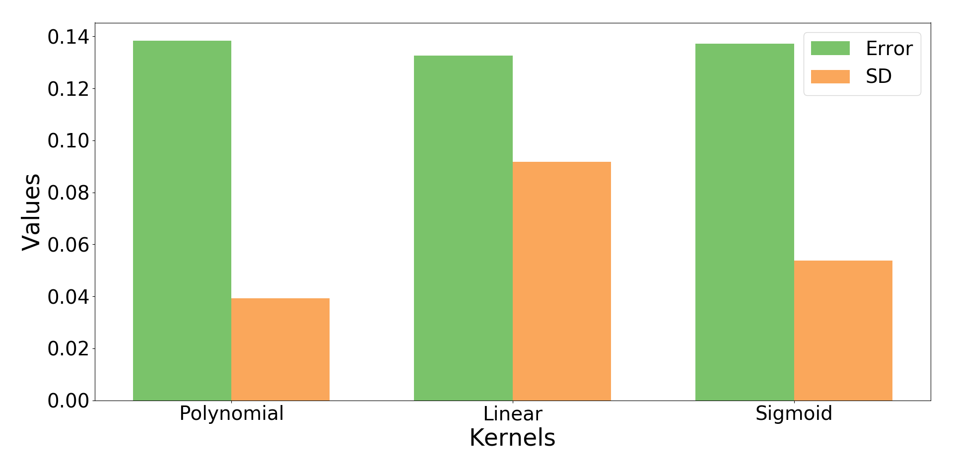
We first examined its performance with different choices of kernel. Results on testing samples averaged over 50 random trials are reported in Figure 1. We see that polynomial kernel achieves the highest prediction fairness, with slightly higher prediction error. Sigmoid kernel is the second best, and linear kernel does not give low disparity. This supports our hypothesis that why fair kernel methods are promising – they construct a complex hypothesis space that is more likely to include models with efficient fairness-accuracy trade-off.

Next, we examined performance with polynomial kernel under different $k$ (number of feature embeddings). Results are shown in Figure 2. We see that smaller $k$ generally leads to higher prediction fairness and slightly higher prediction error. The former phenomenon implies that only the least eigenvectors of problem (6) can effectively minimize the mean discrepancy between two groups. The latter is easy to understand – higher feature dimension provides more information for building an accurate prediction model. However, the variation versus $k$ seems quite limited, suggesting our method has robust classification performance.

We will show how to derive (6) by solving (3) under constraints (4) and (5). Recall that $\eta=\sum_{i=1}^{n}\alpha_{i}\phi(x_{i})$ where $\alpha_{i}$’s are unknown parameters. Rewrite the objective in (3) as

$\displaystyle\begin{split}J(\eta)&=\left|\left|\frac{1}{n_{u}}\sum_{i=1}^{n_{u}}\langle\phi(x_{i}),\eta\rangle-\frac{1}{n_{p}}\sum_{i=n_{u}+1}^{n}\langle\phi(x_{i}),\eta\rangle\right|\right|^{2}\\ &=\frac{1}{n_{u}^{2}}\left(\sum_{i=1}^{n_{u}}\langle\phi(x_{i}),\eta\rangle\right)^{2}+\frac{1}{n_{p}^{2}}\left(\sum_{i=n_{u}+1}^{n}\langle\phi(x_{i}),\eta\rangle\right)^{2}\\ &\quad-\frac{2}{n_{u}n_{p}}\left(\sum_{i=1}^{n_{u}}\langle\phi(x_{i}),\eta\rangle\right)\left(\sum_{i=n_{u}+1}^{n}\langle\phi(x_{i},\eta\rangle\right)\\ &=\frac{\alpha^{T}K_{u}^{T}K_{u}\alpha}{n_{u}^{2}}+\frac{\alpha^{T}K_{p}^{T}K_{p}\alpha}{n_{p}^{2}}-\frac{2\alpha^{T}K_{u}^{T}\mathbf{1}_{u}\mathbf{1}_{p}^{T}K_{p}\alpha}{n_{u}n_{p}}\\ &=\alpha^{T}M\alpha=J(\alpha),\end{split}$

(17)

where $M$ is a symmetric matrix defined as

$$M=\frac{1}{n_{u}^{2}}K_{u}^{T}K_{u}-\frac{2}{n_{u}n_{p}}K_{u}^{T}\mathbf{1}_{u}\mathbf{1}_{p}^{T}K_{p}+\frac{1}{n_{p}^{2}}K_{p}^{T}K_{p},$$

(18)

matrix $K_{u}\in\mathbb{R}^{n_{u}\times n}$ has $k(x_{i},x_{j})$ at row $i$ column $j$ and matrix $K_{p}\in\mathbb{R}^{n_{p}\times n}$ has $k(x_{n_{u}+i},x_{j})$ at row $i$ column $j$; $\mathbbm{1}_{u}\in\mathbb{R}^{n_{u}}$ and $\mathbbm{1}_{p}\in\mathbb{R}^{n_{p}}$ are vectors of ones, and $\alpha=[\alpha_{1},\ldots,\alpha_{n}]$.

Next, it is easy to verify that constraint (4) staisfies

$$\eta^{T}\eta=\alpha^{T}K\alpha=1,$$

(19)

where $K\in\mathbb{R}^{n\times n}$ is the standard Gram matrix.

Thus we need to solve

$$\min_{\alpha}J(\alpha)\quad s.t.\ \alpha^{T}K\alpha=1.$$

(20)

The Lagrange function is

$$L(\alpha,\lambda)=J(\alpha)+\lambda(\alpha^{T}K\alpha-1).$$

(21)

Setting $\frac{\partial L(\alpha,\lambda)}{\partial\alpha}=0$ and solving for $\alpha$ gives (6).

Here, we show why solution to (9) is also a solution to the eigen-problem (6). Let $\alpha$ be the coefficient vector for the first feature embedding $\eta$ (known), and $\alpha^{\prime}$ be the coefficient vector of the second embedding $\eta^{\prime}$ (unknown). The new constraint when learning $\eta^{\prime}$ can be written as

$$\eta^{T}\eta^{\prime}=\left(\sum_{i=1}^{n}\alpha_{i}\phi(x_{i})\right)\left(\sum_{i=1}^{n}\alpha^{\prime}_{i}\phi(x_{i})\right)=\alpha^{T}K\alpha^{\prime}=0.$$

(22)

Thus we need to solve

$$\min_{\alpha^{\prime}}\ J(\alpha^{\prime})\quad s.t.\ (\alpha^{\prime})^{T}K\alpha^{\prime}=1,$$

(23)

and

$$(\alpha^{\prime})^{T}K\alpha=0.$$

(24)

The Lagrange function is

$$L(\alpha^{\prime},\lambda_{1},\lambda_{2})=J(\alpha^{\prime})+\lambda_{1}((\alpha^{\prime})^{T}K\alpha^{\prime}-1)+\lambda_{2}\alpha^{T}K\alpha^{\prime}.$$

(25)

Setting $\frac{\partial L(\alpha^{\prime},\lambda_{1},\lambda_{2})}{\partial\alpha^{\prime}}=0$ and left-multiplying both sides by $\alpha^{T}$,

$$\alpha^{T}M\alpha^{\prime}-2\lambda_{1}\alpha^{T}K\alpha^{\prime}-\lambda_{2}\alpha^{T}K\alpha=0.$$

(26)

Since $\alpha^{T}K\alpha^{\prime}=0$ and $\alpha^{\prime T}K\alpha^{\prime}=1$, we have

$$(\alpha^{\prime})^{T}M\alpha=\lambda_{2}.$$

(27)

Further, from (6) we know $\alpha$ is a generalized eigenvector of $M$ satisfying $M\alpha=\lambda K\alpha$. Thus (27) becomes

$$(\alpha^{\prime})^{T}M\alpha=(\alpha^{\prime})^{T}\lambda K\alpha=\lambda(\alpha^{\prime})^{T}K\alpha=0=\lambda_{2},$$

(28)

where the second equality is due to the new constraint (22).

Comparing (21) and (25), with $\lambda_{2}=0$, we see $\alpha$ and $\alpha^{\prime}$ have the same Lagrange function. Thus it is easy to show they are solution to the same generalized eignproblem (6).

References

- [1] J. Angwin, J. Larson, S. Mattu, and L. Kirchner, “Machine bias: There’s software used across the country to predict future criminals. and it’s biased against blacks,” ProPublica, 2016.
- [2] M. Hoffman, L. B. Kahn, and D. Li, “Discretion in Hiring*,” The Quarterly Journal of Economics, 2017.
- [3] B. F. Klare, M. J. Burge, J. C. Klontz, R. W. V. Bruegge, and A. K. Jain, “Face recognition performance: Role of demographic information,” IEEE Transactions on Information Forensics and Security, 2012.
- [4] M. D. Cunningham and J. R. Sorensen, “Actuarial models for assessing prison violence risk: Revisions and extensions of the risk assessment scale for prison (rasp),” Assessment, 2006.
- [5] Press et al., “Preparing for the future of artificial intelligence,” 2016.
- [6] R. Zemel, Y. Wu, K. Swersky, T. Pitassi, and C. Dwork, “Learning fair representations,” in ICML, 2013.
- [7] M. Feldman, S. A. Friedler, J. Moeller, C. Scheidegger, and S. Venkatasubramanian, “Certifying and removing disparate impact,” in KDD, 2015.
- [8] T. Calders, A. Karim, F. Kamiran, W. Ali, and X. Zhang, “Controlling attribute effect in linear regression,” ICDM, 2013.
- [9] Kamishima, A. Akaho, and Sakuma, “Fairness-aware classifier with prejudice remover regularizer,” in ECML-PKDD, 2012.
- [10] C. Dwork, M. Hardt, T. Pitassi, O. Reingold, and R. Zemel, “Fairness through awareness,” in Innovations in Theoretical Computer Science Conference. ACM, 2012.
- [11] D. McNamara, C. S. Ong, and R. C. Williamson, “Provably fair representations,” CoRR, vol. abs/1710.04394, 2017.
- [12] S. Samadi, U. Tantipongpipat, J. Morgenstern, M. Singh, and S. Vempala, “The price of fair pca: One extra dimension,” in NIPS, 2018.
- [13] A. Pérez-Suay, V. Laparra, G. Mateo-García, J. Muñoz-Marí, L. Gómez-Chova, and G. Camps-Valls, “Fair kernel learning,” in Joint European Conf. Machine Learning and Knowledge Discovery in Databases, 2017.
- [14] M. Olfat and A. Aswani, “Convex formulations for fair principal component analysis,” CoRR, vol. abs/1802.03765, 2019.
- [15] B. Cao, D. Shen, J.-T. Sun, Q. Yang, and Z. Chen, “Feature selection in a kernel space,” in ICML, 2007.
- [16] A. Gretton, K. M. Borgwardt, M. J. Rasch, B. Schölkopf, and A. Smola, “A kernel two-sample test,” JMLR, 2012.
- [17] J. Huang, A. Gretton, K. Borgwardt, B. Schölkopf, and A. J. Smola, “Correcting sample selection bias by unlabeled data,” in NIPS, 2007.
- [18] S. J. Pan, J. T. Kwok, Q. Yang et al., “Transfer learning via dimensionality reduction.” in AAAI, 2008.
- [19] A. Gretton, A. J. Smola, J. Huang, M. Schmittfull, K. M. Borgwardt, and B. Schölkopf, “Covariate shift by kernel mean matching,” 2009.
- [20] Y. Grandvalet and S. Canu, “Adaptive scaling for feature selection in svms,” in NIPS, 2002.
- [21] J. Tang, S. Alelyani, and H. Liu, “Feature selection for classification: A review,” in Data Classification: Algorithms and Applications, 2014.
- [22] L. Yang, S. Lv, and J. Wang, “Model-free variable selection in reproducing kernel hilbert space,” JMLR, 2016.
- [23] B. Schölkopf, A. Smola, and K.-R. Müller, “Kernel principal component analysis,” in International Conf. Artificial Neural Networks, 1997.
- [24] A. Chouldechova, “Fair prediction with disparate impact: A study of bias in recidivism prediction instruments,” Big data, 2017.
- [25] F. Pedregosa, G. Varoquaux, A. Gramfort, V. Michel, B. Thirion, O. Grisel, M. Blondel, P. Prettenhofer, R. Weiss, V. Dubourg, J. Vanderplas, A. Passos, D. Cournapeau, M. Brucher, M. Perrot, and E. Duchesnay, “Scikit-learn: Machine learning in Python,” JMLR, 2011.
VI Appendix
VI-A Derivation of Eigen-Problem (6)
VI-B Derivation of the Solution to (9)