A Bayesian Hierarchical Model for Criminal Investigations
Abstract
Potential violent criminals will often need to go through a sequence of preparatory steps before they can execute their plans. During this escalation process police have the opportunity to evaluate the threat posed by such people through what they know, observe and learn from intelligence reports about their activities. In this paper we customise a three-level Bayesian hierarchical model to describe this process. This is able to propagate both routine and unexpected evidence in real time. We discuss how to set up such a model so that it calibrates to domain expert judgments. The model illustrations include a hypothetical example based on a potential vehicle based terrorist attack.
1 Introduction
How to better support police to prevent terrorist attacks continues to be a major political
concern due to continued violence
perpetrated by extremists Europol 2018; Allen and Dempsey 2018.
In contrast to the majority of terrorist incidents in the latter half of the twentieth century which were executed by
known organised terrorist groups with substantial planning and sophistication, more recent attacks have often involved
individuals or small groups targeting civilians in public places using basic equipment such as vehicles, guns and knives
Europol 2018; Lindekilde et al. 2019. Consequentially this entails less sophistication in materials, planning and execution.
In terms of analysing how to understand and prevent terrorism, criminologist focus has shifted
from “individual qualities (who we think terrorists ‘are’) to …
what lone-actor terrorists do in the
commission of a terrorist attack and how they do it” Gill 2012. Gill, referencing
Horgan 2005, notes “it is useful to view each terrorist offence as comprising of a series of
stages”.
The case studies of lone-actor terrorists have been analysed extensively both qualitatively and quantitatively
for insight into background and preparatory behaviours, vulnerability indicators,
radicalisation patterns, and modes of attack planning Bouhana and Wikstrom 2011; Corner et al. 2019; Lindekilde et al. 2019; Bouhana et al. 2016.
These studies emphasize that the small number and heterogeneity of cases make rigorous scientific examination of
associative and causal relationships extremely difficult. As they indicate it is vital, therefore,
to utilise structure from existing domain expertise on the
relationships between observable data, preparatory activities, and attack modes in any probabilistic
analysis of the progression of an individual to an attack.
Probabilistic models, including Bayesian graphical models, have been used for
modelling “comprehension and decision making of law enforcement personnel with respect to
terrorism-centric behaviours” Regens et al. 2015, in a terrorist cell actor-event network analysis Ranciati et al. 2017,
for “rapid detection of bio-terrorist attacks” Fienberg and Shmueli 2005,
for spatio-temporal terrorism analyses Clark and Dixon 2019; Python et al. 2019, and in a “systems analysis approach
to setting priorities among countermeasures” against terrorist threat Pat-Cornell and Guikema 2002.
Bartolucci et al. 2007 apply a multivariate Latent Markov model to the analysis of criminal trajectories: their focus
is on identifying the model structure given longitudinal data on individuals’ criminal convictions and discrete covariates
such as gender and age band; the latent states are an individual’s “tendency to commit” certain types of crime.
It is within this context that
we present a new class of Bayesian models to dynamically infer the progression of an individual through discrete
stages towards a criminal attack. These models have been developed through close discussions over several years
with a number of different policing agencies.
To our knowledge this approach is novel and complements the existing research.
1.0.1 Overview of the model
A suspect within a subpopulation of interest to the police, , is believed to be planning a serious
criminal attack against the general public. Typically will need to
step through various stages of preparation before perpetrating this crime.
During this progression police will have the opportunity to observe and
evaluate ’s status through their record, updated throughout
an investigation by sporadic intelligence reports and routine observations
of ’s activities. A dynamic Bayesian model is uniquely placed to provide decision
support for such policing activities. It provides a framework within which
to encode criminological theories, domain knowledge
available about , for example his police record and personal modus
operandi, and also draw in evidence from noisy streaming
data about observed by police.
All these features are integrated into a single dynamic probability model. The
model we build in this paper tracks the probability lies in
certain states or makes a transition from one state into another at any given time. These
probabilities help to guide interventions and resource allocations.
To be operational such a Bayesian model must be constructed so that current
prior information in a given suspect ’s record can be quickly updated
not only in the light of routine surveillance but
also unexpected sources. So, for example, police may well be monitoring
the phone log of someone suspected of a serious crime. But within an
investigation direct information sporadically comes to light about what
is doing – unexpected sightings, overheard statements of intent, and so on. It would be
unreasonable to assume that this type of information, often critical to a
correct appraisal of ’s status, could have been forecast and accommodated into any
prior model specification. Any methodology we design for this domain
therefore needs to be open to manual intervention West and Harrison 1997.
Police will then be able to input these unpredicted new sources
of information into the system and so improve the probability assessments of
the Bayesian model. A three level hierarchy facilitates this
openness property.
At the deepest level lies a Reduced Dynamic Chain Event Graph (RDCEG).
This is a
graphically based model drawn from a particular subclass of
finite state semi-Markov processes customised to model
transition processes in a subpopulation of the general public Shenvi and Smith 2018.
This deepest level provides a framework for
expressing the probability judgements of police concerning ’s
current threat status.
The intermediate level of our hierarchy concerns intelligence police
might acquire concerning ’s enacted intentions. When a suspect is
at a particular stage of a criminal pathway, in order to engage in that step
of criminality or alternatively to progress to the next step, a set of
associated tasks needs to be completed. Intermittent intelligence reports often
inform these. Because these are explicit components of the hierarchical
model propagating such information corresponds to simple conditioning. A
vector of tasks whose components form a signature of various states
of criminal intent and capability constitutes the variables that lie on the
intermediate layer of the hierarchy.
The surface layer of the model then links these tasks to the intensities of
certain activities that can be routinely observed by the police if they have
the necessary resource and permissions. In the absence of direct information
about ’s engagement in tasks, signals from predesigned filters
provide vital information about what might be doing.
For example suppose the task concerns ’s intent to travel to a
region to learn how to bomb. Then a filter that measures the intensity of the
suspect’s engagement in searching airline websites would give a noisy signal
of his booking a flight. Such information is imperfect: may book a
flight directly from an airport or to have chosen not to fly to the
destination. And of course a high intensity in such activity could be
entirely innocent: may be booking a vacation, for
example. Such measures are nevertheless obviously informative. Appropriately
chosen filters of these data streams provide the surface level of our
Bayesian hierarchy. The usual Bayesian apparatus then provides a formal and
justifiable framework around which police can logically and defensibly propagate information about .
Formally describing states by collections of tasks within generic Bayesian
models supporting criminal investigations is, to our knowledge, novel.
However it is interesting that Ferrara et al. 2016 proposed a similar approach
albeit less formally expressed and in a more restricted domain: the
discovery of recruiters to radicalisation to extreme violence from Twitter
communications. By performing a number of thought experiments with domain
experts these authors successfully extracted a collection of tasks that a
recruiter would need to engage in to be effective. Although an innocent
non-recruiter, such as an academic or journalist, might happen to engage in
some of the tasks in this collection they would be unlikely to
engage in all of these tasks simultaneously. The authors then related
this vector to various easily extracted meta data signals that could be
routinely extracted from an enormous dataset. This provided an analogue of the types of filter of a
routinely applied observation vector we discuss later here.
In the next section we describe the RDCEG and demonstrate through some
simple examples how it can be used to translate domain experts’ judgements
into a latent probability model at the deepest level of a hierarchy. We also
illustrate sets of tasks that lying in a particular state or
transitioning between states might
entail. Our core methodology is described in Section 3. We propose a
collection of assumptions, elicited from domain experts, about the ways
criminal progressions associate to tasks, and how the intensities
synthesise various sources of routine measurements of engagement in each
of these tasks given background circumstances. Given these assumptions we
are able to propagate not only routine indirect but also unexpected direct
information about ’s current activities to obtain posterior
probabilities about ’s current position.
The resulting propagation algorithms
are straightforward to enact. However the inputs of the
model: both the structural prior information and the prior parameter
distributions embellishing them need to be carefully specified if the
methodology is going to be operationalised. In Section 4 we outline how we
do this.
In this setting to explore the methods using known data on given suspects as
illustrations is clearly unethical. However it is still possible to
demonstrate how the system works in various hypothetical situations whose
distributions are informed by publically available data and elicited
judgements. Therefore in Section 5 we illustrate the way the system is able to
update the state probabilities of an individual under suspicion of a potential attack. We describe
the different task sets we have used and the construction of routine filters
and test these against a two scenarios. In the concluding section we
discuss how we are now extending the methodology to model threatening
subpopulations of the general public where estimation and model selection
algorithms can also be built to better understand the developing processes.
2 The RDCEG for criminal escalation
2.1 Introduction
Chain event graphs (CEGs) are now an established tool for modelling discrete
processes where there is significant asymmetry in the underlying development
see e.g. Barclay et al. 2013; Barclay et al. 2014; Collazo and Smith 2016; Cowell et al. 2014; Görgen and Smith 2018; Collazo et al. 2018. Dynamic
versions of these processes, using analogous semantics, first appeared in
Barclay et al. 2015. However formal extensions of these classes to model
open populations have only recently been discovered Smith and Shenvi 2018 and developed
Shenvi and Smith 2018; Shenvi and Smith 2019. We briefly review and illustrate the main properties of this class as they
apply to the hierarchical model developed here. We refer the reader to the
references above for more details.
The RDCEG we use in this paper is a particular family of semi-Markov process that can be
expressed by a single graph. Each represented state is called a
position. In our domain there is an absorbing state - called the
neutral state that enters when presenting no future threat
of perpetrating the given crime. The practical challenge
is to find a way to systematically construct the set of
positions so that the embedded Markov assumptions are faithful to expert
judgements. In Barclay et al. 2015 and Shenvi and Smith 2018 we describe how this can
be done. We take a natural language description from domain experts and re-express this as a
potentially infinite tree. We then translate this tree into an
equivalent graph . For the purposes above we will
henceforth assume this to have a finite number of vertices.
A position is connected by
a directed edge into another in the graph of an RDCEG iff there is a positive
probability that the next transition from will be into .
Typically although the transition probabilities are fairly stable,
the time it takes to make a transition is not. Therefore we need to express this expert judgement
as a semi-Markov rather than Markov process. The graph is one that on
the one hand is often found to be transparent and natural to our users but
on the other has a formal Bayesian interpretation. So this elicited graph
provides a vehicle to move seamlessly from an expert elicitation into a more
formal family of stochastic processes.
The RDCEG developed in Shenvi and Smith 2019 was designed to be applied to public
health processes where could often be observed directly.
For criminal processes this is not usually possible. Therefore for crime modelling an RDCEG
process typically remains latent and any prior to posterior analysis of
the suspect’s positions needs a little more sophistication. The hierarchical
structure we define in the next section provides the framework for this update. We give some simplified
illustrations below of such RDCEGs.
2.2 A criminal RDCEG and its tasks
We describe an RDCEG, Figure 1, for a politically motivated murder plot illustrating the relationship between its states and tasks: the lowest and intermediate levels in our hierarchical model.
Example 2.1.
Electronic posts directly observed by the police suggest woman is plotting to kill a certain political figure by shooting them. At any time could lie in a number of positions. In positions and she is trained to shoot () in and not () and will own a gun () - position and or not () when in positions and . Each edge and each vertex in the RDCEG below can be associated to different collections of tasks. For example the vertex is associated with the task “attempt murder”; the edges and are associated with the task “acquire gun”. If she cannot shoot she could next choose to learn how next: from a state where she currently owns a gun () or not (,). Alternatively if she currently has no gun then she could next try to acquire one, either when trained to shoot or not. At any point in this process she may enter the neutral state : for example the target may die through other natural or unnatural circumstances, may change her intention, she may be arrested the police having gained enough evidence to charge her. Note that only once she has a gun and can shoot - state - can she attempt the murder by locating and then approaching the target. Implicitly as there is no state “commit murder”, once in the “attempt murder” state she either enters the neutral state or re-enters the “trained to shoot, has gun” state : entering implies she has failed that particular attempt and may try again; entering implies that either she failed and cannot make any further attempts or she succeeded and poses no threat to any other individual. The relevant RDCEG and a table describing the positions, edges, and tasks are given in Figure 1 and Table 1.
| States | Description / State Tasks | Edges | Edge Tasks |
|---|---|---|---|
| plot ends | |||
| can’t shoot, no gun | acquire gun | ||
| train to shoot | |||
| can’t shoot, has gun | train to shoot | ||
| lose gun | |||
| trained to shoot, no gun | acquire gun | ||
| trained to shoot, has gun | locate and approach target , | ||
| lose gun | |||
| attempt murder | fail and escape |
The RDCEG does not have any positions such that there exists two or more edges between them and thus it is simply a subgraph of the state transition graph of a semi-Markov process defining the dynamic where the absorbing state and all edges into it are removed. All states in the process other than appear as vertices. The absorbing state is not depicted for three reasons:
- •
By definition an RDCEG contains the absorbing or “drop-out” state with edges from any position leading to it so depicting would be informationally redundant
- •
Not depicting it and the multiple edges into it reduces visual clutter on the graph
- •
Also by definition once the individual enters they are no longer of interest: hence we focus attention on the active positions by eliding it from the visual depiction
Tasks can be associated to one or more edges or states: here “acquire gun” is associated with the edges and . The structure of the transition matrix, with states of a semi-Markov process with a configuration of zeros given below. The starred entries represent probabilities that need to be added to complete the matrix.
Note this RDCEG has translated the verbal police description above into a
semi-Markov process. It can be elaborated into a full semi-Markov model
by eliciting or estimating the probabilities in
and the holding times. In the above, because of the sum to one
condition, we have eight functionally independent transition probabilities.
To complete the specification of this stochastic process it is necessary to
define the holding time distributions associated with the active states
i.e. how long we believe the suspect will stay in their current state
before transitioning into another. These probabilities and the
parameters of the holding time distributions may well themselves be
uncertain. However of course within a Bayesian analysis their distributions
can be elicited or estimated in standard ways O’Hagan et al. 2006.
The implicit Markov hypotheses of a given RDCEG are of course typically
substantive. One critical issue is that its positions/states define the
only aspects of the history of the suspect that are asserted relevant
to predicting her or his future acts. The art of the modeler is to elicit positions
in such a way that these Markov assumptions are faithful to the expert
judgements being expressed. However because the methodology is fully
Bayesian, experts can be interrogated as to the integrity of these
assumptions just as they can be for other graphical models
Smith 2010. In this way we can iterate towards a model which is
requisite Phillips 1984. The process of query, critique, elaboration and
adjustment is precisely why this bespoke graphical representation is such a
powerful tool. In particular a faithful structural model of the domain
information can be discovered Smith 2010 before numerical
probabilities are elicited or estimated: see e.g. Wilkerson and Smith 2018; Collazo et al. 2018.
2.3 From tasks to routinely observed behaviour
Sometimes solid police intelligence, for example from an informant, will
confirm that is engaged in a particular task. But at other times
only echoes of a task will be seen by police. Suppose is suspected
of being at a stage where they need to accomplish the task of selecting a
target location for a bombing or vehicle attack. They might be observed travelling to what
the police assess might be a potential target to check timings, the density
of people at the venue and its defences activities. This visitation by might have been recorded on CCTVs. In addition or instead,
might inspect Google maps of the attack area and the route to it or
contact like-minded collaborators by phone or electronic media for advice.
So indirect evidence engages in such a task can come from a
variety of media and platforms.
Even such incomplete and disguised signals can be usefully filtered from
complex incoming data about the suspect, albeit with considerable associated
uncertainty. The further a suspect currently is from the main focus of an
investigation the more indirect information will be. However even then the
composition of a collection of weak signals the police are allowed to see
may still provide enough information to significantly revise the evaluation
of the threat posed by a particular individual.
The hierarchical structure we describe below enables us to draw together all
these different types of evidence. If direct information about the tasks a
suspect is engaging in is available then, because such tasks are explicitly
represented within our model, we can simply condition on this information
and so refine our judgements. The Bayesian hierarchical model simply
discards the weaker indirect information to focus on what is known.
Otherwise the model uses filters of the indirect signals police can
see to infer what tasks might be engaging in to help
inform police of ’s position.
3 The structure of the hierarchical task model
3.1 Introduction
Henceforth assume that the RDCEG correctly specifies the
underlying process concerning . To build the propagation algorithms
we first define our notation.
Let be the random variable taking as possible values the states of -
the subpopulation of interest - at time where are the vertices/positions/active
states of and the inactive/neutral state. At any time , might enact one or more of tasks associated to one or more of
the positions or alternatively to
a transition from one position into another . So let
denote the task vector : a vector of binary
random variables where , , indicates that is enacting task at time .
Let denote an indicator on a subset . Then the tasks a suspect
engages in at a given time can be represented by events of the form
.
Direct positive evidence that
lies at position is provided by tasks whose indices lie in
and when is transitioning along the edge by tasks whose indices lie in where are the indices of tasks associated
with the state and are the indices of tasks associated with edges into state and thus
and are both subsets of index set of tasks11
1
For
example in of Section 2.2,
where is “attempt murder”
and is where is “locate target” and is “approach target”.
.
Note that the sets
typically do not form a partition of : tasks can be simultaneously suggestive that lies in one of a number of different active positions.
Occasionally police may also acquire negative evidence from learning
that a suspect - thought to have just before lain in position or be
transitioning along - ceases to perform any of the
associated tasks. From observing the absence of these tasks they might then
infer that might have transitioned either to or a
different active state adjacent to in . Similar
negative inferences might also be made indirectly from learning that stops engaging in all tasks associated with an edge emanating from .
With these issues in mind therefore, let
where
| (1) | |||||
| (2) |
Thus is the set of tasks which can positively
discriminate from when the corresponding components take
the value . The set of tasks in can negatively discriminate:
when taking the value they indicate that
has ceased to engage in tasks associated with preceding positions and is not
engaging in any tasks suggestive of leaving . The set
is then the set of indices of all tasks in any way relevant to .
For each of the component tasks we associate a vector of
observations of a set of related actions:
.
Let be all the routinely observable data on
so each is a projection from to .
It will usually be necessary to work with a filter22
2
Filter in the sense of a function attempting to
identify a signal from noisy data of these data
streams. So let denote
real functions of these processes and set .
3.1.1 Modelling hidden or disguised data
One issue in modelling serious crime is that data concerning a suspect is
often hidden, lost, disguised or even be the result of the use of a decoy. This
means that the data streams are often intentionally corrupted. However, in
contrast to models that describe the data streams directly, our state space
model can conceptually accommodate such disruptions: see West and Harrison 1997.
Guided by police expert judgement, we can explicitly model the processes designed to disguise or
deceive through an appropriate choice of sample distribution of
observations given each task.
Informed missingness using CEGs has already been successfully
applied in a public health study Barclay et al. 2014. Binary variables were introduced indicating the missingness
of readings on mental disability and visual ability for each individual in the Mersey cerebral palsy cohort.
The data set including these missingness variables were used to find the best-fitting structural CEG
model and from this context specific inferences were made on whether the data were MAR, MCAR or
MNAR33
3
Missing at Random, Missing Completely at Random, or Missing Not at Random see Rubin 1976.
In our application we could similarly apply binary variables
for the missingness of any of the routinely observable data in ,
and moreover, as also discussed in Barclay et al. 2014, introduce
categorical variables for the possible reason for missingness: such as hidden, lost, disguised. The presence of certain
patterns of data along with the absence of other data could then influence the probability that certain tasks
were being done despite being hidden or disguised which then would inform the latent state .
Alternatively or additionally
we could explicitly include deception tasks for the hiding of or disguising data and
use the above mentioned patterns of data and missing data to perform inference on the probabilities that
these deception tasks were being done. This is all, however, beyond the scope of this paper.
3.2 The hierarchical model
3.2.1 The conditional independence structure defining the hierarchy
Because by definition and through the process defined above we would like perfect task information to override all such indirect information we will henceforth assume task sufficiency. This states that for all time
| (3) |
where represents the filtration of the past data until but not including time . This clearly implies that for all time
| (4) |
Ideally we would prefer the filter we use to be sufficient for too i.e. that for all time
| (5) |
Then there would be no loss in discarding information in
not expressed in . In what we henceforth present, since
we develop recurrences only concerning and not we
implicitly assume condition 5.
Although condition 5 is a heroic one, in our examples a well-chosen one
dimensional time series of intensities ,
performs well even when these are chosen to be linear in the records of
the component signals . One advantage of this
simplicity is that the role of the filter can be explained and if necessary
adapted by the user, perhaps even customising this filter to their own
personal modus operandi and judgements.
Again for simplicity we henceforth assume that any filter will be a Markov task
filter i.e. that for all
| (6) |
This assumption is a familiar one made for dynamic models; see e.g. West and Harrison 1997. It assumes that once the task is known, no further past information about past will add anything further useful for predicting the future. This assumption enables us, for particular choices of sample distributions, to use all the established recurrences for dynamic state space models - in particular those from dynamic switching models so excellently summarised in Frühwirth-Schnatter 2008. Here our RDCEG probability model specifies such a switching mechanism.
3.2.2 Defining tasks to be fit for purpose
Our interpretation of requires that if suspect is known to be either neutral or in any active state then the only components in that helpfully discriminates between these two possibilities must lie in . The assumption Task set integrity demands is defined so that for all
| (7) |
This is equivalent to requiring that
is a function only of where denotes the set of indices not in . Task set integrity is always satisfied by setting but of course for transparency and computational efficiency ideally is chosen to be a small subset of . Providing the divisor is not zero, task set integrity holds whenever
is a function of only through . So by writing the prior and posterior log -odds as
and the loglikelihood ratio of task vector ,
then a little rearrangement gives us an adaptation of the usual Bayesian linear updating equation linking posterior and prior odds viz:
| (8) |
Note that equation (7) holds in particular whenever it is a simple task vector; i.e. has the property that for any time and
| (9) |
Property 9 holds whenever the other tasks are useless for discriminating any threat position from : the probability engages in these tasks does not depend on these other tasks. In this case the term vanishes and
| (10) |
For practical reasons we have often found it convenient to decompose into functions of components in and respectively. When these are disjoint and conditionally independent given - as in practice we find is often a plausible assumption then
| (11) |
where
Note here that, by definition, , takes its maximum value when and takes its maximum
value when
The equations (10) are now sufficient to calculate
the probability that is in each of the positions given our evidence, using the familiar invertible
function from log odds to probability: see Smith 2010.
3.2.3 Model Assumptions concerning routine observations
For our chosen filtered sequence designed to pick up the different
tasks associated with a criminal process let
Then a simple but bold type of Naive Bayes assumption is to assume that filter is pure: i.e. that for any set containing as a component
| (12) |
Then Bayes Rule and task set integrity implies that within tasks
whilst across tasks
| (13) |
where
Let the prior and posterior odds be respectively denoted by
and let . Then
and from the above
| (14) |
For any set we can therefore calculate
| (15) |
where the Law of Total Probability implies that for
| (16) |
Here the position probabilities over tasks calculated from equation (14) are averaged over the different tasks possibly explaining the data, weighting using the posterior probabilities given in equation (15). Note that it is easy to check that these indirect observations provide less discriminatory power than when tasks are observed directly. The assumptions above therefore provide us with a formally justifiable propagation algorithm for updating the probabilities of a suspect’s likely criminal status. We next turn to how we might calibrate the model to the expert judgements we might elicit from criminologists, police and technicians about the probable relationships between criminal status, what they might try to accomplish and how this endeavour might be reflected through how they communicate.
4 The elicitation process
4.1 Introduction
Copying the standard protocols for the elicitation of a Bayesian Network: see e.g. Korb and Nicholson 2010, as in e.g. Wilkerson and Smith 2018 our process begins with the elicitation of structure. We perform a sequence of three structural elicitations for each of the three levels. These can proceed almost entirely using natural language descriptions of the process. Because the representation of the structure of each of the levels is formal and compatible with a probability model the structural elicitation can take place before the model is quantified. This is extremely helpful because structural information is typically much easier to elicit faithfully than quantitative judgments. The RDCEG defining this structure, the list of tasks and how these might interrelate and then the choice of filter of the routine observations follows:
- 1.
First the decision analyst elicits the positions of the process via the careful conversion of natural language expressions within the domain experts’ description of the process into the topology of a RDCEG - often somewhat more nuanced than the ones we discussed above and in the example below.
- 2.
Second the positions and edges of this RDCEG are then associated to elicited portfolios of tasks.
- 3.
Finally each task is associated with the way domain experts and police believe might behave in order to carry out these tasks, including how they might choose to disguise these actions and so what signals might be visible when enacts a task.
We now briefly outline each of these steps in turn in a little more detail.
4.2 Choosing an appropriate RDCEG
Firstly, when eliciting a RDCEG we aim to keep the number of positions
as small as possible within the constraint that they are sufficient to
distinguish relevant states. The choice of topology should reflect what is known
about the development of the modelled criminal behaviour.
Positions may depend on the history, environmental and personality
profile covariates exhibited by a suspect. Relevant population studies of
criminal behaviours are often helpful here. Based on historical cases,
criminologists’ analyses Gill 2012 and discussions with practitioners,
we have found that the coarsest
type of model - an illustration of such given in the next section - of
different types of attack and concerning different people - are often
generic.
Secondly positions need to be well defined enough to pass the Clarity Test
Howard 1988; Smith 2010. This is achieved by demanding that the
suspect could, if they were so minded, place themselves in a particular
position. Such categories are often syntheses of standard scales used by
social workers and probation workers across the world. Many examples of
these types of categorisations, based on fusing various publicly available
categorisations - for example those found in the training manuals of social
workers in detecting people threatening to eventually perpetrate acts of
severe violence - are given in Smith and Shenvi 2018.
Thirdly positions must be defined such that for each position there is a collection of tasks
associated with it that jointly informs whether the suspect is in that position or transitioning from that position
to another position. A stylised example of
this association was given earlier in this paper and we will illustrate the
process in more detail in the next section with a deeper
illustration.
Once the RDCEG has been drawn its embedded assumptions can be queried by
automatically generating logical deductions concerning the implications of
the model. If such deductions appear implausible to relevant domain experts
then positions need to be redefined and graphs redrawn until they are. The
ways of iterating until a model is requisite and the nature of these
deductions is beyond the scope of this paper but are discussed in Collazo et al. 2018.
The final step in the elicitation of the RDCEG will be the prior conditional
probabilities associated with the positions and the hyperparameters of the
holding times. Suitable generic methods for this
elicitation are now very well established: see e.g. O’Hagan et al. 2006; Smith 2010 and these need little adaptation to be
applied. Note, in particular, that the methods described for
the elicitation of the position probabilities in the RDCEG are essentially
identical to those for the CEG as for example discussed in a chapter of Collazo et al. 2018.
4.3 Elicitation of portfolios of tasks
4.3.1 Clustering the tasks
The next elicitation process is to take each position
in turn and a list of associated tasks conditional on
being known to lie in that position. The questions we might ask
would be something like “Now suppose that you happen to learn that
lies in position . What behaviours/tasks would you expect them to
perform that would be different from what they would typically do were they
neutral?” We try to ensure that either ’s engagement in such tasks
could be learned through intelligence or alternatively be indicated through
certain filters.
Typically in well designed models we specify tasks so that they are as specific to only a small
proportion of ’s active states. This makes them as discriminatory as
possible. Note that each component of must be
defined sufficiently precisely - i.e. pass the clarity test for
to be able to divulge its value if so
inclined; see Smith and Shenvi 2018.
We have found it useful to toggle between specifying positions and
specifying tasks: sometimes aggregating positions if they appear associated
with the same sets of tasks or splitting a position into a set of new ones
if a finer definition can discriminate between one position and another. It
is also sometimes helpful to readjust the definition of tasks once we have
elicited possible signals.
Once the task sets are requisite Phillips 1984; Smith 2010 we need to
specify the various odds ratios against the neutral state. We illustrate this in the next section.
4.3.2 Simplifying assumptions that can ease task probability elicitation
Although the log score updating formulae (equations 8, 10)
are simple ones, to evaluate the log odd scores above can
demand a great many probabilities, both of each task given its associated
position and of seeing that task performed if were neutral, to be
elicited or estimated. This can destabilise the system unless various simplifying
assumptions are made.
Conditional on an active position we recommend that the first
probability to be elicited is when is engaging in all the
tasks in the portfolio of tasks associated with . We then use this elicitation to
benchmark the probability that is engaging in a subset of these
tasks. To calculate the odds of the portfolio against the neutral suspect,
a default assumption that is sometimes appropriate is simply to assume that
people will engage in these probabilities independently- a naive Bayes
Assumption Smith 2010 for the neutral suspect. In this case for any time
and
It is easy to check that when a portfolio contains more than one task, and when such
an assumption is valid, it can provide the basis of a very powerful
discriminatory tool. This is because the divisor in the relevant odds
reduces exponentially with the number of tasks whilst in the denominator
does not: see e.g. Smith and Shenvi 2018 for an example of this.
Of course in some instances this naive Bayes assumption may not be appropriate. It will then need to be substituted. When population statistics
associated with public engagement in different task activities are available
these can be used to verify this assumption or form the basis of
constructively replacing it.
4.4 Choosing an appropriate filter of routine data streams
Typically we would like the components of to measure an intensity of activity related to a
position or edge task. In this sense we would therefore like to factor out
all signals that might be considered typical of ’s innocent
activities so that we can focus on the incriminating signals. The full data
stream collected on
tends to be a highly non-stationary multivariate time series. However we
strive to construct the filter so that the stochastic dependence it exhibits is explained solely by ’s engagement in certain tasks (see equation (6)). This
filter is clearly dependent both on population level signals and what we
know about ’s personality. We therefore usually need expert
judgments to choose so that
it is fit for purpose.
There are some generic features that are worth introducing at this stage.
First in the case of edge tasks we typically observe something different
than before as begins to enact a new task in order to make a
transition. So some components of will be defined as
first differences of derived series. Secondly indicative observations may
also need to be smoothed from the past - either because what we see may
forewarn a task is about to be enacted, or simply because short term
averages - for example any measure of intensity of communication - will
often be better represented by an average over the recent past rather than
by an instantaneous measure.
To construct our hierarchical model we typically loop around the bullets
below:
- 1.
Reflect on what functions of the vector of observable data available to the police might help indicate that a suspect really does lie in a particular task rather than other related innocent activities, . This choice should be informed by the ease at which such signals can be filtered but also how easy it might be for a criminal to disguise that signal were they to learn that the chosen candidate filter was being used.
- 2.
Using expert judgments and any survey data available, reflect on what the distribution of might be were the suspect actually engaged in the particular task and if they were not. Thus specify
- 3.
Check that these two distributions are not close to one another. If not return to the first step.
Finally in many instances of such police work routine measurements concerning suspects are typically recorded and reported over fixed periods of time. This means that the filtered observation sequence is a discrete time filter. For modelling purposes it has been necessary to define the deep stochastic process as semi-Markov. However the semi-Markov structure with holding times and transition probabilities specified will retain the Markov structure over the fixed time points. This means once appropriate transformations are applied standard updating rules associated with Markov switching models are then valid Frühwirth-Schnatter 2008: see Appendix B.
5 A vehicle attacker example
5.1 States
We now give a more detailed example of a vehicle attacker that illustrates the three level hierarchical model of latent states, tasks, and routinely observable data. We specify the states of the RDCEG to be:
| (17) |
where N is “Neutral”, A is “ActiveConvert”, T is “Training”, P is “Preparing”, and M is “Mobilised”. Based on existing information about the suspect we assign prior probabilities to each state as shown in Figure 2; implicitly the prior probability for the elided “Neutral” state is . Based on knowledge about such attacks we hypothesize that the suspect may transition from A to T or P, from T to P, from P to M, and from M back to P. These transitions are indicated by the directed edges between the vertices on said figure. The weights labelling the transitions are the probabilities of transitions from the source vertex to the destination vertex conditional on a transition having occurred (i.e. the entries labelled in Table 5 in Appendix B). The probability of transition into the “Neutral” state from any represented state is implied by the sum of all the emanating edges’ probabilities summing to one. This is in contrast to Shenvi and Smith 2018 where the transition probabilities are conditional on not moving to the absorbing state. This prior RDCEG is used in all the examples in this section.
5.2 Tasks
We hypothesize the tasks relevant for these positions, i.e. the tasks that are related to which position the suspect is in, are:
where:
is Engaging with Radicals
is Engaging in Public Threats
is Making Personal Threats
is Fewer Public Engagements in Radicalisation
is Fewer Contacts with Family and Friends
is Securing Monetary Resources
is Learning to Drive Large Vehicle
is Obtaining Vehicle
is Reconnaissance of Target Locations
is Moving to Target Location
For each position , a particular subset of the above tasks are taken to be indicators that the suspect
is there. is the index set for this subset and we need to
specify the distribution for each position.
Appendix A details a methodology for this
specification that makes the model discriminatory and Table 4 shows the resulting probabilities used.
5.3 Routinely observable data
The data used to estimate the probabilities that the suspect is engaging in any particular
task or tasks are varied and various and may change as technologies and data gathering methods change.
In addition as new evidence is gained and the threat level of a suspect increases the authorities
may decide to increase monitoring and hence gain more and new types of data. Therefore having
the tasks intermediate the positions from the observed data is desirable
for both model structural reasons and practical data abstraction purposes. We denote
the observable data as a -dimensional vector process in discrete time .
In general we assume . In this example, however,
several of the components are count data, such as the number of
times such events are observed in a given period, so that:
.
We set here:
: radical website visits
: physical meetings with known radicals
: electronic meetings with known radicals
: meetings with trained radicals
: meetings with known cell members
: seen at radical demonstrations
: contacts with non-radicals
: public threats made
: personal threats made
: increase in known financial resources
: decrease in known financial resources
: obtaining large vehicle driving licence
: vehicle dealer or rental website visits
: vehicle dealer or rental physical visits
: E-visits to target locations
: physical visits to target locations
: statements of intent
: legacy statements
As described in Section 3 we assume that for each task we can construct a filter
of the relevant data: Here we define the function :
where is a normalisation44 4 we subtract a pre-defined mean and divide by a pre-defined standard deviation estimated by investigators’ judgement, experience and historical data o and is the cardinality of the index set of components of dependent on the task. We could also set additional components of to be changes over time of other components of and thus monitor drops or spikes in, for example, communication levels with known radicalisers, or with family and friends. We specify the relationship between the observable data and the tasks in Table 2 where the entry indicates whether the th variable is relevant data for the th task.
| Observable | ||||||||||
|---|---|---|---|---|---|---|---|---|---|---|
| RadWebVisits | 1 | 0 | 0 | 1 | 1 | 0 | 0 | 0 | 0 | 0 |
| PhysicalMeetsWithRadicals | 1 | 0 | 0 | 0 | 1 | 0 | 0 | 0 | 0 | 0 |
| E-MeetsWithradicals | 1 | 0 | 0 | 1 | 1 | 0 | 0 | 0 | 0 | 0 |
| MeetTrainedRadicals | 1 | 0 | 0 | 0 | 1 | 0 | 0 | 0 | 0 | 0 |
| MeetCellMembers | 1 | 0 | 0 | 0 | 1 | 0 | 0 | 0 | 0 | 0 |
| SeenAtRadicalDemonstrations | 1 | 0 | 0 | 0 | 1 | 0 | 0 | 0 | 0 | 0 |
| ContactsWithNonRadicals | 0 | 0 | 0 | 1 | 0 | 0 | 0 | 0 | 0 | 0 |
| PublicThreatsMade | 0 | 1 | 0 | 0 | 0 | 0 | 0 | 0 | 0 | 0 |
| PersonalThreatMade | 0 | 0 | 1 | 0 | 0 | 0 | 0 | 0 | 0 | 0 |
| IncreaseInFinances | 0 | 0 | 0 | 0 | 0 | 1 | 1 | 1 | 0 | 0 |
| DecreaseInFinances | 0 | 0 | 0 | 0 | 0 | 0 | 1 | 1 | 0 | 0 |
| ObtainLGVLicence | 0 | 0 | 0 | 0 | 0 | 0 | 1 | 0 | 0 | 0 |
| CarDealerWebHits | 0 | 0 | 0 | 0 | 0 | 0 | 0 | 1 | 0 | 0 |
| CarDealerPhysicalVisits | 0 | 0 | 0 | 0 | 0 | 0 | 0 | 1 | 0 | 0 |
| E-VisitsToTargetLocations | 0 | 0 | 0 | 0 | 0 | 0 | 0 | 0 | 1 | 0 |
| VisitsToTargetLocations | 0 | 0 | 0 | 0 | 0 | 0 | 0 | 0 | 1 | 0 |
| LegacyStatements | 0 | 0 | 0 | 0 | 0 | 0 | 0 | 0 | 0 | 1 |
| StatementOfIntent | 0 | 1 | 1 | 0 | 0 | 0 | 0 | 0 | 0 | 1 |
5.4 Specifications of the distributions of the task set given position and task set likelihood
For each position we set the probability that all the tasks in that position’s task set are being done to . The individual probabilities that each task is being done given the suspect is in the neutral state are specified in the column labelled “Neutral” in Table 3. The log odds interpolation methodology detailed in Appendix A is then used to construct the probabilities that no tasks or less than all the tasks were being done. For example, as shown in the Table 3, for the “Mobilised” position, the tasks “Engaging in public threats”, “Making personal threats”, “Reconnaissance of target locations”, and “Moving to target location” are relevant. Table 4 has the resulting probabilities for each point of .
| ActiveConvert | Training | Preparing | Mobilised | Neutral | |
| State_Task_Index_Sets | |||||
| EngageWithRadicalisers | 1 | 0 | 0 | 0 | 0.020 |
| EngageInPublicThreats | 0 | 0 | 1 | 1 | 0.001 |
| MakePersonalThreats | 0 | 0 | 1 | 1 | 0.001 |
| RedPubEngInRad | 1 | 1 | 0 | 0 | 0.600 |
| RedCntctWthFmlyFrnds | 1 | 0 | 0 | 0 | 0.300 |
| ObtainResources | 1 | 1 | 0 | 0 | 0.300 |
| LearnToDrive | 0 | 1 | 0 | 0 | 0.300 |
| ObtainVehicle | 0 | 1 | 1 | 0 | 0.200 |
| ReconnoitreTargets | 0 | 0 | 1 | 1 | 0.100 |
| MoveToTarget | 0 | 0 | 0 | 1 | 0.200 |
| Cardinality | 4 | 4 | 4 | 4 | |
| p+ | 0.400 | 0.400 | 0.400 | 0.400 | |
| p0 | 0.001 | 0.011 | 0.00000002 | 0.00000002 | |
| 1.051 | 2.076 | 0.332 | 0.331 |
| ActiveConvert | Training | Preparing | Mobilised | |
|---|---|---|---|---|
| State_Task_Index_Sets | ||||
| np_0 | 0.00108 | 0.01080 | 0.00000002 | 0.00000002 |
| np_0001 | 0.00475 | 0.01341 | 0.00112 | 0.00112 |
| np_0010 | 0.00475 | 0.01341 | 0.00112 | 0.00112 |
| np_0011 | 0.02319 | 0.02742 | 0.01860 | 0.01860 |
| np_0100 | 0.00475 | 0.01341 | 0.00112 | 0.00112 |
| np_0101 | 0.02319 | 0.02742 | 0.01860 | 0.01860 |
| np_0110 | 0.02319 | 0.02742 | 0.01860 | 0.01860 |
| np_0111 | 0.11019 | 0.09277 | 0.12098 | 0.12098 |
| np_1000 | 0.00475 | 0.01341 | 0.00112 | 0.00112 |
| np_1001 | 0.02319 | 0.02742 | 0.01860 | 0.01860 |
| np_1010 | 0.02319 | 0.02742 | 0.01860 | 0.01860 |
| np_1011 | 0.11019 | 0.09277 | 0.12098 | 0.12098 |
| np_1100 | 0.02319 | 0.02742 | 0.01860 | 0.01860 |
| np_1101 | 0.11019 | 0.09277 | 0.12098 | 0.12098 |
| np_1110 | 0.11019 | 0.09277 | 0.12098 | 0.12098 |
| np_1111 | 0.40000 | 0.40000 | 0.40000 | 0.40000 |
| ntp | 1.00000 | 1.00000 | 1.00000 | 1.00000 |
For simplicity we used shifted asymmetric logistic functions to construct the task set likelihood functions : see equations (18). The shift parameters and the growth rate parameters , were used to construct functions that were relatively unresponsive when but sharply responsive when . An illustration of the form of these functions is provided in Figure 3 for the one and two-dimensional cases i.e. when there are one or two tasks in the task set ; this is purely for ease of plotting: as shown in Table 3 four dimensional task sets were used in the example scenarios.
| (18) |


5.5 Scenarios
We illustrate the propagation of probabilities through the model based on scenarios of simulated data. We use the same framework as above and manually set the routinely observed data through 24 weekly time steps to examine how the currently parameterised model behaves under each scenario.
Scenario 5.1.
In this scenario the suspect increases their web visits to target locations from week 8 and their physical visits to target locations from the week 21; they are in constant communication with known radicals and there is an increase in their finances followed by a decrease in first few weeks, during which time they are seen to be visiting car dealers electronically and physically. They make public and personal threats and in the last weeks of the period the threatening data increases with a legacy statement and a statement of intent. Figures 4(a), 5(a), 5(c) show the increase in threat level resulting from this scenario.
Scenario 5.2.
The suspect’s communications and possible training / preparing type data linearly decreases from initial levels similar to scenario 5.1 to zero over the 24 weeks. Moreover there are no threats made during the whole period. Figures 4(b), 5(b), 5(d) show the decreasing threat level resulting from this scenario.


5.6 Eventual probability of mobilisation
For any individual suspect or group of suspects the medium to long-term probabilities of mobilisation is of key interest and can aid as a model diagnostic tool. We can estimate this by using the semi-Markov transition matrix to evolve the current probabilities. The RDCEG in this section has the neutral state as the single absorbing state hence asymptotically the probability of this state will go to one; However in the practical medium term we can examine the behaviour of the active positions including the mobilised state. Under the configuration of the priors and the edge probabilities as in Figure 2 and with the holding time distribution set to a constant for the set time period of equal to one week (as used in the examples above), the qualitative behaviour of the RDCEG’s state probabilities can be seen in Figures 6(a) and 6(b). Figures 6(c) and 6(d) show the long term behaviour under alternative specifications where the mobilised position is another absorbing state: the suspect once having mobilised and executed the attack cannot transition to any of the other states including the neutral state. The reasoning behind this latter configuration is an assumption that once the individual has mobilised this entails an attack and the end of this particular police case.


6 Model diagnostics
6.1 Robustness to RDCEG structure specification
The graph representation of the RDCEG, that is the set of states and the directed edges between them, form the structure
of the RDCEG that is meant to faithfully represent the possible pathways of individuals towards, in this application,
acts of terrorism. The actual structure chosen is based on historical cases, existing research by criminologists and
discussions with practioners and is predicated on the assumption that the states are “self-identifiable”
that is that the actual individual would be able to place themselves in one of these states at any given time.
Assuming such an approach is valid, without being able to actually look into an individual’s mind, we are
liable to mis-specify
the structure: for example construct states that could meaningfully and usefully be split into finer sub-states, or
have a set of states that should be collapsed into one state; or have edges where they should not exist or have edges
missing. Whether the set of states are “correct to the individual’s mind” is arguably less
relevant for our purposes than whether the set of states are a useful discretisation of the individual’s potential pathway
from the investigators’ perspective; and for this we can be directly guided.
It is still of use to analyse the sensitivity of behaviour and results to changes in the structure chosen.
To this end we examine the effect of using different sets of states and different edges by using the same data sets
with different RDCEG structures.
We coursen the RDCEG used in Section 5 by collapsing the “Training” state into the “Preparing” state,
and then separately refine the RDCEG by splitting the “Preparing” state in two states: “Preparing for a
Vehicle Attack” and “Preparing for a Bomb Attack”, so that we have two new alternative RDCEG structures to
compare with the original. We expand the task sets and data and run
two new data scenarios involving a potential joint vehicle and bomb attack on these two new structures along with
the original structure giving in total six sets of results.
Results for this analysis along with details of the scenarios are given in Appendix D and
Appendix C.
The impacts on the posterior probabilities are as expected: the “Neutral” state’s probability is relatively
unchanged and the probability mass of the coarsened state is roughly the sum of the finer states in each
example under both scenarios.
In contrast to our elicited RDCEG structure, Shenvi and Smith 2019 construct an RDCEG structure explicitly from
data on individuals within an open population using a hierarchical clustering algorithm and Bayes Factor based model
selection in health care settings: recurrent falls in the elderly in the context of care services and drug effects on
early epilepsy cases.
6.2 Sensitivity analysis
To improve our understanding of the behaviour and robustness of the model to subjective inputs, and to identify key
parameters that merit extra analysis to determine their optimal value, we
perform sensitivity analysis against a base scenario. The model is high dimensional in the sense that the number
of configurable parameters is large: so for the time being this analysis has focussed on the state prior probabilities
and the holding distributions the latter of which are key to determining the speed of transition.
We tested the sensitivity of the evolution
of the state probabilities applying both moderate and large shifts to the state priors. We
performed a similar analysis shifting the holding time distribution parameter which represents the probability
of a transition from state to in a given time period (here one week) given that an edge exists from
to .
For moderate changes in
priors, increasing the prior for a less threatening state has an initial effect but is outweighed by any data that
indicates threat; whilst an increase in prior for a threat state accelerates the effect of threat data.
For extreme increases in prior for the active states the prior does dominate the evolution; but for the “Neutral”
state the initial very high prior is subsequently outweighed by data. See Appendix E for figures.
7 Discussion
In this paper we have described a novel three level hierarchical model that utilises at its deepest level
an RDCEG modelling the state of a suspect within the stages of a potential attack.
We illustrated how such an analysis can
synthesise information concerning that suspect, through sets of tasks to produce snap shot
summaries of the likely position of this person and the current threat they
might present.
Currently, working with various domain experts, we are in the process of
constructing a suite of RDCEG templates and their associated tasks
Smith and Shenvi 2018. These describe different criminal processes
associated with assaults or violence against the general public, indexed by
type of crime, that build on existing criminological
models. This type of technology has already been well
developed for BNs within the context of forensic science Aitken and Teroni 2004; Mortera and Dawid 2017 and has established frameworks of processes linking
activities with evidence. The structure we use here helps in this
development because only the top layer of the hierarchy usually needs
regular refreshing: the possible positions and associated tasks are fairly
stable over time. We hope that within this paper we have illustrated
that, just as in forensic science, such methods are both promising and
feasible. Indeed the harmonisation of this class of models to forensic
analogues means that evidence applied within an investigation can be
coherently integrated into case reports associated with criminal proceedings
if the suspect does attempt to perpetrate a crime.
In the next phase of this programme, building on these models of individual
suspects, we are developing a network model for the stochastic evolution of open populations
of violent criminals. This issue is complicated by the fact that many suspects are working
in teams and often coordinated. This dependence structure and communications between indivuduals
therefore have to be carefully modelled for such models to be realistic. However this more
challenging domain is also a potentially very fertile one - where standard
estimation of hyperparameters associated with different units and the
Bayesian selection of the most promising models can begin to be applied. The
challenge is that series are frequently disrupted so the systematic
estimation of their hyperparameters is hard and needs strong prior
information to be effective.
The eventual objective is for the hierarchical model for individuals described in this paper and the network model
described in the paragraph above, to be incorporated into a decision theoretic framework that also models the action
space and objectives of the authorities. This would aim to aid investigators decide which actions to take; such as
which cases to prioritise, or to deprioritise to free up resources, which cases to increase surveillance on,
and which cases to make which kind of interventions on;
all in order to minimise the expectation of a multi-attribute loss function over incidents, casualties, public terror
etc., given the constraints of resources, personal freedom, democratic legitimacy and proportionality.
Moreover the actions of the authorities in terms of preventative measures, defence of targets and
pursuit methods will influence the actual decisions and trajectories of the suspects as is
documented in case reports (see for example Gill 2012). These recursive aspects
introduce game-theoretic ideas into the models which complicate the inferential process and probability
propagation. This work has to be done in conjunction with
the authorities in order to properly represent a realistic, constrained action space,
to elicit a realistic loss function, and to gain insight on the dynamic interplay between investigator and investigated.
Thus the work we present in this paper is the first phase of a longer programme working with practitioners
that eventually aims to provide a theoretically valid, practically useful, and legally defensible system
to support the prevention of acts of extreme radical violence.
Acknowledgements
This work was funded by The Alan Turing Institute Defence and Security Project G027. We are grateful for the comments of two anonymous referees and the associate editor which greatly improved this paper.
Appendix A Task probabilities given position
Some settings that keep elicitation of task probabilities to the minimum whilst appearing to provide good discriminatory power in most circumstances are given below. For each state , let
be the probability that all the positive tasks and none of the negative tasks are being done given the position is . For definitions of see Equations 1 in Section 3. We define and elicit tasks in such a way that
i.e. given someone is in active position then the probability
that in is engaged in all the tasks that are
positive indicators and none of the tasks that are negative indicators is non-negligible. We also assume
that the less the engagement in the positive tasks the smaller the probability lies in this active state and the contrary for the negative tasks.
Let and
denote the cardinality of the sets
and .
Suppose where is
the cardinality of
and where is the cardinality of .
Then
| (19) |
so is the number of tasks being done in plus those not being done in . Let the log odds be:
| (20) |
Then under the Naive Bayes assumption of Section 4 for , we set
| (21) |
Then the full set of probabilities for any such and can be generated by interpolating:
where is constrained such that the resulting probabilities sum to one. This setting has the property that preserves the sorts of monotonicity we require for the comment above.
Appendix B The semi-Markov transition matrix and resulting recurrence equations
We now explicitly model the process as a continuous time process, still with discrete state space. We still assume
that we observe data at discrete sequential times: , but we model explicitly that the
suspect may transition between states between or at these observation times.
Thus the discrete time process is embedded in a continuous time semi-Markov process
, .
Assume that the time interval is short so that at most one transition has occurred between
and . Conditioning on the event that there has only been one transition, let
represent the probability of a transition from during the time interval
, where is the holding distribution for the position.
Let represent the probability that the suspect will transition to the position
from position given there has been exactly one state transition.
Then the components of the transition matrix are given by:
Using the RDCEG of the vehicle attacker in Section 5, we have and as in Table 5 with denoting edge probabilities: i.e. the probability of transition from the source vertex to the destination vertex conditional on a transition having occurred.
| Neutral | ActiveConvert | Training | Preparing | Mobilised | |
|---|---|---|---|---|---|
| N | 0 | 0 | 0 | 0 | 0 |
| A | 0 | 0 | |||
| T | 0 | 0 | 0 | ||
| P | 0 | 0 | 0 | ||
| M | 0 | 0 | 0 | ||
| Neutral | ActiveConvert | Training | Preparing | Mobilised | |
| N | 1 | 0 | 0 | 0 | 0 |
| A | 0 | ||||
| T | 0 | 0 | |||
| P | 0 | 0 | |||
| M | 0 | 0 |
Under the assumption that the observation times are frequent enough that at most one transition could occur between them, the filtering equations to update the position probabilities given the change in time and the observed data are
| (22) | |||
| (23) | |||
| (24) |
Equation (23) updates the position probabilities given the observed data at time whilst Equation (24) transitions the position probabilities over a small time interval according to the transition matrix . Now we ease the assumption that observation times are frequent enough that we can exclude the possibility of more than one state transition between them. For ease of exposition and notation we assume that the intervals between observation times are a multiple of , ie
for every and for some . Here we take the holding time distributions as time-homogenous although in future work we plan to use inhomogenous distributions. With homogeneity the transition matrix between observation times is then simply the appropriate power of , i.e.
Then Equation (24) can be written as:
| (25) |
The prior and posterior log odds formulae used in Equations 8 and 10 of the main paper are amended to be based on rather than and to function as filtering recurrence equations based on . Suppressing to simplify the notation we obtain:
The the loglikelihood ratio of becomes
and the update formula on the log odds is
| (26) |
Appendix C Multiple Attack Method Scenarios
These scenarios are used for the model diagnostic analyses of Appendix D and E.
- •
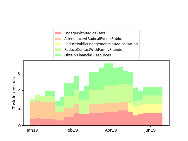
Scenario A: The suspect is seen to make radical statements both in public and privately including public threats; they increase their meetings with known radicals and other suspected cell members; they sell assets, increase their financial resources, hire a vehicle, investigate bomb-making and technical web-sites; they are seen electronically and physically visiting target locations and are then seen to be making large financial expenditures. The normalised data is displayed as stacked bar charts in Figures 7(a) to 9(b); and the resulting task intensities are shown in Figures 10(a) to 11(b).
- •
Scenario B: The suspect reduces public and private contact and engagement with radicals and at no time makes and radical statements or threats.




Appendix D RDCEG robustness
We use the model as described in Section 5 as the base RDCEG structure, base prior state probabilities and base holding distribution. We use Scenarios A and B from Appendix C to analyse the effect on the probability evolution through time under changes in the RDCEG structure. The results are illustrated in Figures 12 to 18


Appendix E Sensitivity analysis
Again we use the model as described in Section 5 as the base RDCEG structure, base prior state probabilities and base holding distribution. We use Scenarios A and B in Appendix C to analyse the effect on the probability evolution through time under changes in the state prior probabilities and changes in the holding distribution parameter . Figure 20 and Tables 6 and 7 illustrate these impacts.


| SubScenario | Prior | t5 | t10 | t15 | t20 | t26 | |
|---|---|---|---|---|---|---|---|
| State | |||||||
| Neutral | a | 0.050 | 0.028 | 0.016 | 0.006 | 0.001 | 0.000 |
| ActiveConvert | a | 0.600 | 0.696 | 0.566 | 0.367 | 0.167 | 0.064 |
| Training | a | 0.200 | 0.178 | 0.235 | 0.242 | 0.221 | 0.108 |
| Preparing | a | 0.100 | 0.068 | 0.119 | 0.235 | 0.380 | 0.398 |
| Mobilised | a | 0.050 | 0.031 | 0.063 | 0.149 | 0.231 | 0.430 |
| Neutral | b | 0.269 | 0.165 | 0.100 | 0.041 | 0.010 | 0.002 |
| ActiveConvert | b | 0.462 | 0.597 | 0.518 | 0.354 | 0.165 | 0.064 |
| Training | b | 0.154 | 0.153 | 0.215 | 0.234 | 0.219 | 0.108 |
| Preparing | b | 0.077 | 0.058 | 0.109 | 0.227 | 0.377 | 0.397 |
| Mobilised | b | 0.038 | 0.026 | 0.058 | 0.144 | 0.229 | 0.429 |
| Neutral | c | 0.038 | 0.020 | 0.012 | 0.005 | 0.001 | 0.000 |
| ActiveConvert | c | 0.692 | 0.773 | 0.660 | 0.462 | 0.228 | 0.091 |
| Training | c | 0.154 | 0.133 | 0.184 | 0.205 | 0.203 | 0.105 |
| Preparing | c | 0.077 | 0.051 | 0.095 | 0.203 | 0.357 | 0.392 |
| Mobilised | c | 0.038 | 0.023 | 0.049 | 0.125 | 0.211 | 0.411 |
| Neutral | d | 0.038 | 0.022 | 0.012 | 0.004 | 0.001 | 0.000 |
| ActiveConvert | d | 0.462 | 0.549 | 0.419 | 0.268 | 0.124 | 0.054 |
| Training | d | 0.385 | 0.350 | 0.431 | 0.438 | 0.405 | 0.226 |
| Preparing | d | 0.077 | 0.055 | 0.092 | 0.180 | 0.298 | 0.356 |
| Mobilised | d | 0.038 | 0.024 | 0.047 | 0.109 | 0.172 | 0.364 |
| Neutral | e | 0.038 | 0.023 | 0.012 | 0.004 | 0.001 | 0.000 |
| ActiveConvert | e | 0.462 | 0.582 | 0.425 | 0.223 | 0.082 | 0.030 |
| Training | e | 0.154 | 0.149 | 0.177 | 0.147 | 0.108 | 0.051 |
| Preparing | e | 0.308 | 0.219 | 0.336 | 0.528 | 0.684 | 0.688 |
| Mobilised | e | 0.038 | 0.027 | 0.051 | 0.098 | 0.126 | 0.231 |
| Neutral | f | 0.038 | 0.023 | 0.011 | 0.003 | 0.001 | 0.000 |
| ActiveConvert | f | 0.462 | 0.588 | 0.412 | 0.196 | 0.071 | 0.018 |
| Training | f | 0.154 | 0.151 | 0.171 | 0.129 | 0.094 | 0.031 |
| Preparing | f | 0.077 | 0.058 | 0.089 | 0.131 | 0.171 | 0.124 |
| Mobilised | f | 0.269 | 0.180 | 0.315 | 0.541 | 0.664 | 0.827 |
| SubScenario | Prior | t5 | t10 | t15 | t20 | t26 | |
|---|---|---|---|---|---|---|---|
| State | |||||||
| Neutral | g | 0.200 | 0.142 | 0.065 | 0.017 | 0.003 | 0.001 |
| ActiveConvert | g | 0.200 | 0.300 | 0.197 | 0.086 | 0.029 | 0.008 |
| Training | g | 0.200 | 0.229 | 0.243 | 0.169 | 0.115 | 0.042 |
| Preparing | g | 0.200 | 0.170 | 0.236 | 0.313 | 0.376 | 0.293 |
| Mobilised | g | 0.200 | 0.158 | 0.260 | 0.414 | 0.477 | 0.656 |
| Neutral | h | 0.962 | 0.943 | 0.875 | 0.635 | 0.234 | 0.050 |
| ActiveConvert | h | 0.010 | 0.020 | 0.026 | 0.032 | 0.022 | 0.008 |
| Training | h | 0.010 | 0.015 | 0.032 | 0.063 | 0.088 | 0.040 |
| Preparing | h | 0.010 | 0.011 | 0.032 | 0.116 | 0.289 | 0.279 |
| Mobilised | h | 0.010 | 0.010 | 0.035 | 0.154 | 0.366 | 0.623 |
| Neutral | i | 0.010 | 0.005 | 0.003 | 0.002 | 0.001 | 0.000 |
| ActiveConvert | i | 0.962 | 0.972 | 0.945 | 0.864 | 0.665 | 0.379 |
| Training | i | 0.010 | 0.010 | 0.017 | 0.028 | 0.044 | 0.033 |
| Preparing | i | 0.010 | 0.008 | 0.021 | 0.065 | 0.180 | 0.283 |
| Mobilised | i | 0.010 | 0.005 | 0.013 | 0.042 | 0.110 | 0.304 |
| Neutral | j | 0.010 | 0.006 | 0.003 | 0.001 | 0.000 | 0.000 |
| ActiveConvert | j | 0.010 | 0.013 | 0.008 | 0.005 | 0.002 | 0.001 |
| Training | j | 0.962 | 0.963 | 0.958 | 0.925 | 0.876 | 0.726 |
| Preparing | j | 0.010 | 0.012 | 0.022 | 0.047 | 0.084 | 0.155 |
| Mobilised | j | 0.010 | 0.007 | 0.010 | 0.023 | 0.037 | 0.118 |
| Neutral | k | 0.010 | 0.008 | 0.003 | 0.001 | 0.000 | 0.000 |
| ActiveConvert | k | 0.010 | 0.017 | 0.008 | 0.003 | 0.001 | 0.000 |
| Training | k | 0.010 | 0.013 | 0.010 | 0.005 | 0.003 | 0.001 |
| Preparing | k | 0.962 | 0.948 | 0.956 | 0.958 | 0.959 | 0.927 |
| Mobilised | k | 0.010 | 0.014 | 0.023 | 0.033 | 0.037 | 0.072 |
| Neutral | l | 0.010 | 0.009 | 0.002 | 0.000 | 0.000 | 0.000 |
| ActiveConvert | l | 0.010 | 0.018 | 0.007 | 0.002 | 0.001 | 0.000 |
| Training | l | 0.010 | 0.014 | 0.009 | 0.004 | 0.002 | 0.001 |
| Preparing | l | 0.010 | 0.016 | 0.018 | 0.020 | 0.025 | 0.018 |
| Mobilised | l | 0.962 | 0.944 | 0.963 | 0.974 | 0.972 | 0.981 |


| State | Prior | t0 | t5 | t10 | t15 | t20 | t26 | |
|---|---|---|---|---|---|---|---|---|
| 0.001 | Neutral | 0.05 | 0.045 | 0.028 | 0.016 | 0.006 | 0.001 | 0.000 |
| ActiveConvert | 0.6 | 0.625 | 0.696 | 0.566 | 0.367 | 0.167 | 0.064 | |
| Training | 0.2 | 0.193 | 0.178 | 0.235 | 0.242 | 0.221 | 0.108 | |
| Preparing | 0.1 | 0.091 | 0.068 | 0.119 | 0.235 | 0.380 | 0.398 | |
| Mobilised | 0.05 | 0.046 | 0.031 | 0.063 | 0.149 | 0.231 | 0.430 | |
| State | Prior | t0 | t5 | t10 | t15 | t20 | t26 | |
| 0.01 | Neutral | 0.05 | 0.045 | 0.028 | 0.015 | 0.005 | 0.001 | 0.000 |
| ActiveConvert | 0.6 | 0.620 | 0.664 | 0.495 | 0.275 | 0.105 | 0.035 | |
| Training | 0.2 | 0.193 | 0.183 | 0.233 | 0.213 | 0.166 | 0.072 | |
| Preparing | 0.1 | 0.096 | 0.092 | 0.184 | 0.346 | 0.495 | 0.475 | |
| Mobilised | 0.05 | 0.046 | 0.033 | 0.072 | 0.161 | 0.233 | 0.417 | |
| State | Prior | t0 | t5 | t10 | t15 | t20 | t26 | |
| 0.1 | Neutral | 0.05 | 0.046 | 0.030 | 0.013 | 0.003 | 0.001 | 0.000 |
| ActiveConvert | 0.6 | 0.567 | 0.404 | 0.138 | 0.030 | 0.005 | 0.001 | |
| Training | 0.2 | 0.198 | 0.201 | 0.150 | 0.060 | 0.023 | 0.005 | |
| Preparing | 0.1 | 0.138 | 0.272 | 0.427 | 0.497 | 0.505 | 0.408 | |
| Mobilised | 0.05 | 0.050 | 0.093 | 0.273 | 0.410 | 0.466 | 0.587 | |
| State | Prior | t0 | t5 | t10 | t15 | t20 | t26 | |
| 0.5 | Neutral | 0.05 | 0.048 | 0.041 | 0.014 | 0.003 | 0.001 | 0.001 |
| ActiveConvert | 0.6 | 0.326 | 0.015 | 0.000 | 0.000 | 0.000 | 0.000 | |
| Training | 0.2 | 0.221 | 0.037 | 0.001 | 0.000 | 0.000 | 0.000 | |
| Preparing | 0.1 | 0.335 | 0.477 | 0.458 | 0.504 | 0.488 | 0.468 | |
| Mobilised | 0.05 | 0.071 | 0.429 | 0.526 | 0.492 | 0.511 | 0.530 |
References
- Aitken and Teroni (2004) Aitken, C. and Teroni, F. (2004). Statistics and the Evaluation of Evidence for Forensic Scientists. Wiley.
- Allen and Dempsey (2018) Allen, G. and Dempsey, N. (2018). “Terrorism in Great Britain: the statistics. Briefing Paper Number CBP7613.” Technical report, House of Commons.
- Barclay et al. (2015) Barclay, L. M., Collazo, R. A., Smith, J. Q., Thwaites, P. A., Nicholson, A. E., et al. (2015). “The dynamic chain event graph.” Electronic Journal of Statistics, 9(2): 2130–2169.
- Barclay et al. (2013) Barclay, L. M., Hutton, J. L., and Smith, J. Q. (2013). “Refining a Bayesian Network using a Chain Event Graph.” Int. J. Approx. Reasoning, 54: 1300–1309.
- Barclay et al. (2014) — (2014). “Chain Event Graphs for Informed Missingness.” Bayesian Anal., 9(1): 53–76.
- Bartolucci et al. (2007)
Bartolucci, F., Pennoni, F., and Francis, B. (2007).
“A Latent Markov Model for Detecting Patterns of Criminal
Activity.”
Journal of the Royal Statistical Society. Series A (Statistics
in Society), 170(1): 115–132.
URL http://www.jstor.org/stable/4623137 - Bouhana et al. (2016) Bouhana, N., Thornton, A., Corner, E., Malthaner, S., Lindekilde, L., B., S., and Perry, G. (2016). “EU FP7 PRIME risk analysis framework.” Technical report, Public version.
- Bouhana and Wikstrom (2011) Bouhana, N. and Wikstrom, P.-O. H. (2011). “Al Qai‘da-influenced radicalisation: A rapid evidence assessment guided by Situational Action Theory.” Rds occasional paper 97, London, England: Home Office Research, Development and Statistics Directorate.
- Clark and Dixon (2019) Clark, N. J. and Dixon, P. M. (2019). “Modeling and Estimation for Self-Exciting Spatio-Temporal Models of Terrorist Activity.” The Annals of Applied Statistics, 12(1): 633–653.
- Collazo et al. (2018) Collazo, R. A., Goergen, C., and Smith, J. Q. (2018). Chain Event Graphs. CRC Press.
- Collazo and Smith (2016)
Collazo, R. A. and Smith, J. Q. (2016).
“A New Family of Non-Local Priors for Chain Event Graph Model
Selection.”
Bayesian Anal., 11(4): 1165–1201.
URL https://doi.org/10.1214/15-BA981 - Corner et al. (2019) Corner, E., Bouhana, N., and Gill, P. (2019). “The multifinality of vulnerability indicators in lone-actor terrorism.” Psychology, Crime and Law, 25(2): 111–132.
- Cowell et al. (2014) Cowell, R. G., Smith, J. Q., et al. (2014). “Causal discovery through MAP selection of stratified chain event graphs.” Electronic Journal of Statistics, 8(1): 965–997.
- Europol (2018) Europol (2018). “Terrorism Situation And Trend Report.” Technical report, European Union Agency for Law Enforcement Cooperation.
- Ferrara et al. (2016)
Ferrara, E., Wang, W., Varol, O., Flammini, A., and Galstyan, A. (2016).
“Predicting online extremism, content adopters, and
interaction reciprocity.”
CoRR, abs/1605.00659.
URL http://arxiv.org/abs/1605.00659 - Fienberg and Shmueli (2005) Fienberg, S. E. and Shmueli, G. (2005). “Statistical issues and challenges associated with rapid detection of bio-terrorist attacks.” Statistics in Medicine, 12(24): 513–529.
- Frühwirth-Schnatter (2008) Frühwirth-Schnatter, S. (2008). Finite mixture and Markov switching models. Springer.
- Gill (2012) Gill, P. (2012). “Tracing the Motivations and Antecedent Behaviors of Lone-Actor Terrorism A Routine Activity Analysis of Five Lone-Actor Terrorist Events.” Technical report, International Center for the Study of Terrorism, The Pennsylvania State University.
- Görgen and Smith (2018)
Görgen, C. and Smith, J. Q. (2018).
“Equivalence classes of staged trees.”
Bernoulli, 24(4A): 2676–2692.
URL https://doi.org/10.3150/17-BEJ940 - Horgan (2005) Horgan, J. (2005). The Psychology of Terrorism. Abingdon: Routledge, first edition.
- Howard (1988)
Howard, R. A. (1988).
“Decision Analysis: Practice and Promise.”
Management Science, 34(6): 679–695.
URL https://doi.org/10.1287/mnsc.34.6.679 - Korb and Nicholson (2010) Korb, K. B. and Nicholson, A. E. (2010). Bayesian Artificial Intelligence, Second Edition. Boca Raton, FL, USA: CRC Press, Inc., 2nd edition.
- Lindekilde et al. (2019) Lindekilde, L., O’Connor, F., and Schuurman, B. (2019). “Radicalization patterns and modes of attack planning and preparation among lone-actor terrorists: an exploratory analysis.” Behavioral Sciences of Terrorism and Political Aggression, 11(2): 113–133.
- Mortera and Dawid (2017)
Mortera, J. and Dawid, A. P. (2017).
“Graphical Models For Forensic Analysis.”
Departmental Working Papers of Economics - University ’Roma Tre’
0224, Department of Economics - University Roma Tre.
URL https://ideas.repec.org/p/rtr/wpaper/0224.html - O’Hagan et al. (2006)
O’Hagan, A., Buck, C. E., Daneshkhah, A., Eiser, J. R., Garthwaite, P. H.,
Jenkinson, D. J., Oakley, J. E., and Rakow, T. (2006).
Uncertain Judgements: Eliciting Expert Probabilities.
Chichester: John Wiley.
URL http://oro.open.ac.uk/17948/ - Pat-Cornell and Guikema (2002) Pat-Cornell, E. and Guikema, S. (2002). “Probabilistic Modeling of Terrorist Threats: A Systems Analysis Approach to Setting Priorities Among Countermeasures.” Military Operations Research, 7: 5–23.
- Phillips (1984)
Phillips, L. D. (1984).
“A theory of requisite decision models.”
Acta Psychologica, 56(1): 29 – 48.
URL http://www.sciencedirect.com/science/article/pii/0001691884900052 - Python et al. (2019) Python, A., Illian, J. B., Jones-Todd, C. M., and Blangiardo, M. (2019). “A Bayesian approach to modelling subnational spatial dynamics of worldwide non-state terrorism, 2010–2016.” Journal of the Royal Statistical Society: Series A (Statistics in Society), 182(1): 323–344.
- Ranciati et al. (2017) Ranciati, S., Vinciotti, V., and Wit, E. C. (2017). “Identifying overlapping terrorist cells from the Noordin Top actor-event network.” arXiv e-prints, arXiv:1710.10319.
- Regens et al. (2015) Regens, J. L., Mould, N., Jensen, C. J., Graves, M. A., and Edger, D. N. (2015). “Probabilistic Graphical Modeling of Terrorism Threat Recognition Using Bayesian Networks and Monte Carlo Simulation.” Journal of Cognitive Engineering and Decision Making, 9(4): 295–311.
- Rubin (1976)
Rubin, D. B. (1976).
“Inference and missing data.”
Biometrika, 63(3): 581–592.
URL https://doi.org/10.1093/biomet/63.3.581 - Shenvi and Smith (2018) Shenvi, A. and Smith, J. Q. (2018). “The Reduced Dynamic Chain Event Graph.” arXiv e-prints, arXiv:1811.08872.
- Shenvi and Smith (2019) Shenvi, A. and Smith, J. Q. (2019). “A Bayesian Dynamic Graphical Model for Recurrent Events in Public Health.” Working paper.
- Smith (2010)
Smith, J. Q. (2010).
Bayesian decision analysis : principles and practice.
Cambridge, UK ; New York: Cambridge University Press.
URL http://wrap.warwick.ac.uk/45002/ - Smith and Shenvi (2018)
Smith, J. Q. and Shenvi, A. (2018).
“Assault Crime Dynamic Chain Event Graphs.”
Working paper.
URL http://wrap.warwick.ac.uk/104824/ - West and Harrison (1997) West, M. and Harrison, J. (1997). Bayesian Forecasting and Dynamic Models (2Nd Ed.). Berlin, Heidelberg: Springer-Verlag.
- Wilkerson and Smith (2018) Wilkerson, R. L. and Smith, J. Q. (2018). “Customised Structural Elicitation.” arXiv e-prints, arXiv:1807.03693.