跳到论文正文
W Papers独立论文阅读器 arXiv:1907.01854 论文正文 计算阅读时间 · 0%
引用这篇论文根据当前论文元数据生成,正式投稿前建议核对。


License: arXiv.org perpetual non-exclusive license
arXiv:1907.01854v1 [math.DS] 03 Jul 2019

Farey Sequences for Thin Groups

Christopher Lutsko∗
∗University of Bristol
   UK
Abstract

The classical Farey sequence of height QQ is the set of rational numbers in reduced form with denominator less than QQ. In this paper we introduce the concept of a generalized Farey sequence. While these sequences arise naturally in the study of discrete (and in particular thin) subgroups, they can be used to study interesting number theoretic sequences - for example rationals whose continued fraction partial quotients are subject to congruence conditions. We show that these sequences equidistribute, that the gap distribution converges, and we answer an associated problem in Diophantine approximation with Fuchsian groups. Moreover, for one specific example, we use a sparse Ford configuration construction to write down an explicit formula for the gap distribution. Finally for this example, we construct the analogue of the Gauss measure in this context which we show is ergodic for the Gauss map. This allows us to prove a theorem about the Gauss-Kuzmin statistics of the sequence.

Key words and phrases: Farey Sequence; Continued Fractions; Equidistribution; Local Statistics; Ford Circles; Patterson-Sullivan Theory.

1 Introduction

Consider the classical Farey sequence of height QQ:

ℱ~Q:={pq∈[0,1):(p,q)∈ℤ^2,0<q<Q},\tilde{\mathcal{F}}_{Q}:=\left\{\frac{p}{q}\in[0,1)\;:\;(p,q)\in\hat{\mathbb{Z}}^{2},0<q<Q\right\}, (1.1)

where ℤ^2\hat{\mathbb{Z}}^{2} denotes the set of primitive vectors in ℤ2\mathbb{Z}^{2}. Naturally this sequence is a fundamental object in number theory dating back to 1802 with its introduction by Haros and subsequent work by Farey and Cauchy. For example, this sequence has connections to the Riemann hypothesis (see for example [LM17]) and plays a fundamental role in Diophantine approximation.

In this paper, we generalize the Farey sequence. For concreteness, one example of such a generalized Farey sequence is given by the following: throughout the paper we use the standard continued fration notation

[a0;a1,…​an]=a0+1a1+1a2+...an[a_{0};a_{1},\dots a_{n}]=a_{0}+\frac{1}{a_{1}+\frac{1}{a_{2}+\frac{...}{a_{n}}}} (1.2)

(see for example [Khi35]) then denote

𝒬4:={[0;a1,…ak]:k∈ℕ,ai∈4ℤ≠0∀i},\mathcal{Q}_{4}:=\left\{[0;a_{1},\dots a_{k}]:k\in\mathbb{N}\;,\;a_{i}\in 4\mathbb{Z}_{\neq 0}\;\forall i\right\}, (1.3)

that is, rationals whose continued fraction expansions involve only multiples (possibly negative) of 44. The generalized Farey sequence in this context is

ℱ^Q={pq∈𝒬4:0<q<Q,gcd(p,q)=1}\widehat{\mathcal{F}}_{Q}=\{\frac{p}{q}\in\mathcal{Q}_{4}:0<q<Q,\;\gcd(p,q)=1\} (1.4)

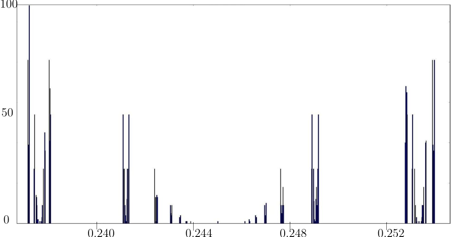
we return to this example in Section 1.1 where we give a geometric interpretation of these sets. To see some of the points of 𝒬4\mathcal{Q}_{4} see Figure 1 on page 1.

Refer to caption
Figure 1: Above we show some of the points in 𝒬4\mathcal{Q}_{4}. The graph was generated as follows: we generated all words of length 1010 (with respect to the two generators applied to ∞\infty). Then separated the interval [0,1)[0,1) into bins of size 10−510^{-5}. The above is a bar chart showing the number of points in each bin. Note that the sequence is supported on a fractal subset of the interval. This does not show ℱ^Q\widehat{\mathcal{F}}_{Q} (as the cut-off is with respect to word length), however will suffice for a qualitative picture.

There is a geometric interpretation of the classical Farey sequence which will play an integral role in this paper. Consider the groups G=PSL⁡(2,ℝ)G=\operatorname{PSL}(2,\mathbb{R}) and Λ:=PSL⁡(2,ℤ)<G\Lambda:=\operatorname{PSL}(2,\mathbb{Z})<G. GG acts on the hyperbolic half-space, ℍ\mathbb{H} via Möbius transformations (see Section 2). As Λ\Lambda is a lattice, there exists a tessalation of ℍ\mathbb{H} into disjoint, finite volume subsets such that Λ\Lambda acts transitively on them. These fundamental domains are not compact as each one contains a point on the boundary ∂ℍ=ℝ∪{∞}\partial\mathbb{H}=\mathbb{R}\cup\{\infty\}, at the end of a cusp. The set of such cuspidal points is exactly

(Λ/Λ∞)​∞=ℚ(\Lambda/\Lambda_{\infty})\infty=\mathbb{Q} (1.5)

(we use GxG_{x} to denote the stabilizer of xx in a group GG). That is, the set of cuspidal points can be written as the Λ\Lambda-orbit of the point at ∞∈∂ℍ\infty\in\partial\mathbb{H} - which corresponds to the rationals. Thus the Farey sequence of height QQ can be written

ℱ~Q={pq∈(Λ/Λ∞)∞:(p,q)∈ℤ^2,0<q<Q}\tilde{\mathcal{F}}_{Q}=\left\{\frac{p}{q}\in(\Lambda/\Lambda_{\infty})\infty:(p,q)\in\hat{\mathbb{Z}}^{2},0<q<Q\right\} (1.6)

- the points in the Λ\Lambda-orbit of the point at ∞∈∂ℍ\infty\in\partial\mathbb{H} with denominator less than QQ. The goal of this paper is to consider a generalization of this setup, where we replace Λ\Lambda by a general (possibly infinite covolume) discrete subgroup. For our example (1.4) the corresponding subgroup is the Hecke group

Γ^=⟨(1401),(01−10)⟩.\widehat{\Gamma}=\left<\left(\begin{array}[]{cc}1&4\\ 0&1\end{array}\right),\left(\begin{array}[]{cc}0&1\\ -1&0\end{array}\right)\right>. (1.7)

Most of our theorems hold for general subgroups. Hence, let Γ<PSL⁡(2,ℝ)\Gamma<\operatorname{PSL}(2,\mathbb{R}) be a general non-elementary, finitely generated subgroup in GG with critical exponent δΓ\delta_{\Gamma}. In our context 1/2<δΓ≤11/2<\delta_{\Gamma}\leq 1 and δΓ\delta_{\Gamma} is equal to the Hausdorff dimension of the limit set of the subgroup (we introduce these definitions in Section 2). Furthermore assume Γ\Gamma has a cusp at ∞\infty and let Γ∞=(Γ/Γ∞)​∞⊂∂ℍ\Gamma^{\infty}=(\Gamma/\Gamma_{\infty})\infty\subset\partial\mathbb{H} denote the orbit of ∞\infty. Hence, Γ∞\Gamma^{\infty} is the set of the cusps located at points on the boundary, isomorphic to ∞\infty. Finally we assume that Γ∞=⟨(1101)⟩\Gamma_{\infty}=\left<\begin{pmatrix}1&1\\ 0&1\end{pmatrix}\right>. I.e that the fundamental domain is periodic with period 11 along the real line. Note that Γ^\widehat{\Gamma} has period 44. However a scaling could be applied to give it period 11 (in order to preserve the continued fraction description we refrain from doing so).

Let

𝒵:={(p,q)∈(0,1)Γ}⊂ℝ2,\mathcal{Z}:=\left\{(p,q)\in(0,1)\Gamma\right\}\subset\mathbb{R}^{2}, (1.8)

denote the analogue of primitive vectors and define

ℱQ:={pq∈[0,1):(p,q)∈𝒵,0<q<Q}={pq∈Γ∞:0≤p<q<Q}.\displaystyle\begin{aligned} \mathcal{F}_{Q}&:=\left\{\frac{p}{q}\in[0,1):(p,q)\in\mathcal{Z},0<q<Q\right\}\\ &=\left\{\frac{p}{q}\in\Gamma^{\infty}:0\leq p<q<Q\right\}.\end{aligned} (1.9)

ℱQ\mathcal{F}_{Q} is the primary object of study for this article, which we call a generalized Farey sequence (occassionally gFs). In Subsection 3.1 we show that asymptotically there exists a constant 0<cΓ<∞0<c_{\Gamma}<\infty such that

|ℱQ|∼cΓ​Q2​δΓ.|\mathcal{F}_{Q}|\sim c_{\Gamma}Q^{2\delta_{\Gamma}}. (1.10)

The goal of the paper is to establish the Theorems in Sections 4 - 9 which we describe briefly here. As the statements of the theorems require the use of fractal measures, we present them formally only after presenting the necessary notation (readers familiar with Patterson-Sullivan theory may wish to skip ahead and see the theorems now). Sections 2 and 3 present some background and preliminary work. Subsequently the main results of the paper are:

  • •

    Counting primitive points: In Section 4 we present a theorem for the equidistribution of the horocycle flow in infinite volume subgroups (proved by Oh and Shah [OS13]). Then we show how this equidistribution result can be used to prove a technical theorem about counting primitive points in a sheared set (Theorem 4.3) and another technical theorem about counting primitive points in a rotated set (Theorem 4.5). These theorems generalize the analogous result for lattices in [MS10].

  • •

    Diophantine approximation by parabolics: We prove two theorems in metric Diophantine approximation in Fuchsian groups. These are the analogues of the Erdös-Szüsz-Turán and Kesten problems in the infinite volume setting. In the classical setting, these problems were solved using homogeneous dynamics by Marklof in [Mar99, Theorem 4.4] and Athreya and Ghosh [AG18]. Moreover Xiong and Zaharescu [XZ06] and Boca [Boc08] solved the problem using number theoretic methods (by applying the BCZ map). Extending classical results in metric Diophantine approximation to the setting of Fuchsian groups is not new and was done by Patterson [Pat76] who proved Dirichlet and Khintchine type theorems for such parabolic points. More recently, for example Beresnevich et. al. [BGSV18] studied the equivalent problems for Kleinian groups.

    In the same section we show that Theorem 4.5 allows us to prove that there is a limiting distribution for the direction of primitive points, 𝒵\mathcal{Z}, as viewed from the origin. This problem has not been addressed in the Euclidean setting except for lattices ([MS10]).

  • •

    Equidistribution of gFs: Theorem 6.1 states that the gFs equidistributes over a horospherical section. In a series of papers ([Mar10], [Mar13]), Marklof showed that the (classical) Farey sequence, when embedded into a horosphere equidistributes on a particular section. This equidistribution theorem was then used to show that the spatial statistics of the Farey sequence converge. This was followed by work of Athreya and Cheung [AC14] who (in dimension d=2d=2) were able to construct a Poincaré section for the horocycle flow such that the return time map generates Farey points. We restrict our attention to proving the equidistribution result in this more general setting. Heersink [Hee17] generalized [Mar10] to certain congruence subgroups of Λ\Lambda (still in the finite covolume setting). Furthermore, the method of [AC14] has been generalized to more general subgroups such as Hecke triangle groups (e.g [Tah19]). However we will not discuss this approach here.

  • •

    Convergence of local statistics: Theorem 7.1, as a consequence of Theorem 4.3 and Theorem 6.1, states that two sorts of local statistics converge in the limit. A corollary of one of these is that the limiting gap distribution exists. This distribution in the classical setting was originally calculated by Hall [Hal70] (and is known as the Hall distribution) and has been studied by many people since. The Hall distribution was originally put into the context of ergodic theory in [BCZ01].

  • •

    An explicit formula for the gap distribution: In Section 8 we restrict to the example Γ^\widehat{\Gamma}. For this example we show that the limiting gap distribution can be explicitly written as an integral over a compact region. While the integral involves a fractal measure this is the first time such an explicit formula has been calculated in the infinite volume setting. There is much interest in finding explicit formula for limiting gap distributions for projected lattice point sets and the infinite covolume analogue. The only instance (to our knowledge) of such explicit examples are those covered in [RZ17]. In that paper Rudnick and Zhang used the relation between Farey points and Ford circles to produce examples for which they could express the limiting gap distribution explicitly (recovering, in one instance, the Hall distribution). In Section 1.1 we show that the Farey sequence for Γ^\widehat{\Gamma} can also be used to generate a (sparse) Ford Configuration which leads to our result.

  • •

    Ergodicity of a new Gauss-like measure: Continuing to work with the example Γ^\widehat{\Gamma}, we show that a new fractal measure takes on the role of the Gauss measure (Theorem 9.2). That is, this measure is ergodic for the Gauss map. As an application we show that this ergodicity implies convergence to an explicit function of the Gauss-Kuzmin statistics in our context. This section takes inspiration from [Ser85] where Series showed how the Gauss measure can be viewed as a projection of the Haar measure on a particular cross-section.

1.1 Ford configurations for Γ^\widehat{\Gamma}

To give some further intuition for generalized Farey sequences, in this section we show that the gFs for Γ^\widehat{\Gamma} admits a simple geometric interpretation which we shall return to in section Section 8. Returning to our example ℱ^Q\widehat{\mathcal{F}}_{Q} - (1.4), note that

Γ^∞=𝒬4.\widehat{\Gamma}^{\infty}=\mathcal{Q}_{4}. (1.11)

To see this, simply note that the two generators in (1.7) correspond to the maps f⁡(x)=x+4f(x)=x+4 and g⁡(x)=−1xg(x)=\frac{-1}{x} which generate these continued fractions.

Consider the action of Γ^\widehat{\Gamma} on an initial configuration of circles in the closure ℍ¯\overline{\mathbb{H}}:

𝒦0:=(𝒞0,𝒞1,𝒞2,𝒞3)𝒞0=ℝ,𝒞1=ℝ+i,𝒞2=C⁡(i/2,1/2),𝒞3=C⁡(i/2+4,1/2)\displaystyle\begin{gathered}\mathcal{K}_{0}:=(\mathcal{C}_{0},\mathcal{C}_{1},\mathcal{C}_{2},\mathcal{C}_{3})\\ \mathcal{C}_{0}=\mathbb{R}\quad,\quad\mathcal{C}_{1}=\mathbb{R}+i\quad,\quad\mathcal{C}_{2}=C(i/2,1/2)\quad,\quad\mathcal{C}_{3}=C(i/2+4,1/2)\end{gathered}

where C⁡(z,r)C(z,r) is a circle located at z∈ℍ¯z\in\overline{\mathbb{H}} of radius rr. We are interested in the resulting sparse Ford configuration, 𝒦:=Γ^​𝒦0\mathcal{K}:=\widehat{\Gamma}\mathcal{K}_{0}, shown in Figure 2. Any group element in Γ^\widehat{\Gamma} can be decomposed into a composition of circle inversions through vertical lines at 00 and 44 and C⁡(0,1)C(0,1) and C⁡(4,1)C(4,1) (these are also shown in Figure 2).

Figure 2: Diagram of a portion of 𝒦\mathcal{K}. The dotted lines represent the circle inversions coresponding to the subgroup Γ^\widehat{\Gamma}. The white circles (including the xx-axis and horizontal line above) represent the initial configuration 𝒦0=(𝒞0,𝒞1,𝒞2,𝒞3)\mathcal{K}_{0}=(\mathcal{C}_{0},\mathcal{C}_{1},\mathcal{C}_{2},\mathcal{C}_{3}). The filled-in circles represent some of the images.

Let 𝒜T\mathcal{A}_{T} denote the set of tangencies with 𝒞0\mathcal{C}_{0} in [0,1][0,1] such that the circle tangent to 𝒞0\mathcal{C}_{0} has diameter larger than T−1T^{-1}. The way we have constructed the packing 𝒦\mathcal{K}, these tangencies are exactly the cuspidal points of the group (i.e the tangencies are located on the orbit Γ^∞\widehat{\Gamma}^{\infty}). Moreover one can easily show if a circle in this packing is tangent to 𝒞0\mathcal{C}_{0} at p/qp/q in reduced form then the diameter is given by 1/q21/q^{2}. Hence 𝒜Q2=ℱ^Q\mathcal{A}_{Q^{2}}=\widehat{\mathcal{F}}_{Q}, i.e the set of tangencies of circles with diameter greater than Q2Q^{2} is exactly the gFs of height QQ.

Given an interval ℐ⊂[0,1]\mathcal{I}\subset[0,1], let 𝒜T,ℐ=𝒜T∩ℐ\mathcal{A}_{T,\mathcal{I}}=\mathcal{A}_{T}\cap\mathcal{I}. We label the elements of 𝒜T={xT,ℐj}j=1#​𝒜T,ℐ\mathcal{A}_{T}=\{x^{j}_{T,\mathcal{I}}\}_{j=1}^{\#\mathcal{A}_{T,\mathcal{I}}} such that xT,ℐj<xT,ℐj+1x^{j}_{T,\mathcal{I}}<x^{j+1}_{T,\mathcal{I}} for all jj. The gap distribution is then

F^T,ℐ(s):=#⁡{i∈[1,#​𝒜T,ℐ):T⁡(xT,ℐj+1−xT,ℐj)≤s}TδΓ^\widehat{F}_{T,\mathcal{I}}(s):=\frac{\#\left\{i\in[1,\#\mathcal{A}_{T,\mathcal{I}}):T(x^{j+1}_{T,\mathcal{I}}-x^{j}_{T,\mathcal{I}})\leq s\right\}}{T^{\delta_{\widehat{\Gamma}}}} (1.14)

for s>0s>0.

In Section 8 we show that the limiting gap distribution can be explicitly calculated as a sum of integrals over compact regions involving a fractal measure presented below. This allows us to show that all gaps have size bigger than s<2s<2 (not just in the limiting case), and to say something more about the regularity of FF and the growth of the derivative.

Remark.

Of course different subgroups generate different sparse Ford configurations and have other interesting relations to continued fractions (and hence Diophantine approximation). We only address this (simplest) example here. That said, our methods generalize without additional effort to any Hecke subgroup of the form Γc=⟨(0c01),(0−110)⟩\Gamma_{c}=\left<\begin{pmatrix}0&c\\ 0&1\end{pmatrix},\begin{pmatrix}0&-1\\ 1&0\end{pmatrix}\right> for c∈ℝ>2c\in\mathbb{R}_{>2} (the corresponding continued fraction description will involve cc rather than 44 and this loses some elegance for non-integer cc).

2 Background - Hyperbolic Geometry

Consider the action of GG on ℍ\mathbb{H} via Möbius transformations: for z∈ℍz\in\mathbb{H} and g=(abcd)∈Gg=\begin{pmatrix}a&b\\ c&d\end{pmatrix}\in G

g​z=a​z+bc​z+dzg=tgz=a​z+cb​z+d.\displaystyle\begin{aligned} &gz=\frac{az+b}{cz+d}\\ &zg=\mathop{}\mathopen{\vphantom{g}}^{t}\kern-0.5ptgz=\frac{az+c}{bz+d}.\end{aligned} (2.1)

Let Xi∈T1​(ℍ)X_{i}\in T^{1}(\mathbb{H}) denote the vector pointing upwards based at ii. Denote

  • •

    K=StabG⁡(i)K=\operatorname{Stab}_{G}(i), hence ℍ≅G/K\mathbb{H}\cong G/K.

  • •

    AA - a one parameter subgroup corresponding to the unit speed geodesic flow, 𝒢r\mathcal{G}_{r}, on T1​(ℍ)T^{1}(\mathbb{H}). For XiX_{i} the action of AA corresponds to multiplication by Φt=(et/200e−t/2)\Phi^{t}=\begin{pmatrix}e^{t/2}&0\\ 0&e^{-t/2}\end{pmatrix}.

  • •

    N−:={n−​(x)=(1x01):x∈ℝ}N_{-}:=\left\{n_{-}(x)=\left(\begin{array}[]{cc}1&x\\ 0&1\end{array}\right):x\in\mathbb{R}\right\}, the contracting horosphere for Φt\Phi^{t}.

  • •

    N+:={n+​(x)=(10x1):x∈ℝ}N_{+}:=\left\{n_{+}(x)=\left(\begin{array}[]{cc}1&0\\ x&1\end{array}\right):x\in\mathbb{R}\right\}, the expanding horosphere for Φt\Phi^{t}.

We identify points in GG with points in T1​(ℍ)T^{1}(\mathbb{H}) via the map g↦g​Xig\mapsto gX_{i} and points in G/KG/K we identify with points in ℍ\mathbb{H} via the map g↦g​ig\mapsto gi.

2.1 Measure Theory on Infinite Volume Hyperbolic Manifolds

To construct the appropriate measures we require the following definitions. For a point u∈T1​(ℍ)u\in T^{1}(\mathbb{H}) denote the forward and backward geodesic projections

u±=limr→∞𝒢r​(u).u^{\pm}=\lim_{r\to\infty}\mathcal{G}_{r}(u). (2.2)

Moreover, for g∈Gg\in G we denote g±=g​(Xi)±g^{\pm}=g(X_{i})^{\pm}. Let ℒ⁡(Γ)⊂∂ℍ\mathcal{L}(\Gamma)\subset\partial\mathbb{H} - the limit set - denote the set of accumulation points of any orbit under Γ\Gamma. A classical result in the field states that the Hausdorff dimension of ℒ⁡(Γ)\mathcal{L}(\Gamma) is the critical exponent δΓ\delta_{\Gamma} ([Sul79]).

Given a boundary point ξ∈∂ℍ\xi\in\partial\mathbb{H} and two points in the interior x,y∈ℍx,y\in\mathbb{H}, define the Busemann function to be

βξ​(x,y):=limt→∞d⁡(x,ξt)−d⁡(y,ξt),\beta_{\xi}(x,y):=\lim_{t\to\infty}d(x,\xi_{t})-d(y,\xi_{t}), (2.3)

where ξt\xi_{t} is any geodesic such that limt→∞ξt=ξ\lim_{t\to\infty}\xi_{t}=\xi. In words, the Busemann function measures the signed distance between the horospheres containing xx and yy based at ξ\xi.

Define a Γ\Gamma-invariant conformal density of dimension δμ>0\delta_{\mu}>0 to be a family, {μx:x∈ℍ}\{\mu_{x}:x\in\mathbb{H}\} of finite, Borel measures on the boundary ∂ℍ\partial\mathbb{H} such that

γ∗μx(⋅):=μx(γ−1⋅)=μγ​x(⋅),d​μxd​μy(ξ)=eδμ​βξ​(y,x),\gamma_{\ast}\mu_{x}(\cdot):=\mu_{x}(\gamma^{-1}\cdot)=\mu_{\gamma x}(\cdot),\hskip 10.00002pt\frac{d\mu_{x}}{d\mu_{y}}(\xi)=e^{\delta_{\mu}\beta_{\xi}(y,x)}, (2.4)

for any y∈ℍy\in\mathbb{H}, ξ∈∂ℍ\xi\in\partial\mathbb{H} and γ∈Γ\gamma\in\Gamma. Patterson [Pat76] (in dimension 22) and Sullivan [Sul79] (in higher dimensions) constructed a Γ\Gamma-invariant conformal density of dimension δΓ\delta_{\Gamma} supported on the limit set ℒ⁡(Γ)\mathcal{L}(\Gamma). We denote this conformal density νx\nu_{x}. Moreover let mx\mathrm{m}_{x} denote the GG-invariant density of dimension 11 (the Lesbegue density).

Given a point u∈T1​(ℍ)u\in T^{1}(\mathbb{H}) let π⁡(u)\pi(u) denote the projection to ℍ\mathbb{H} and let s=βu−​(i,π⁡(u))s=\beta_{u^{-}}(i,\pi(u)). From there define the following measures:

  • •

    The Burger-Roblin measure

    d​mB​R​(u)=eδΓ​βu−​(i,π⁡(u))​eβu+​(i,π​(u))​d​νi​(u−)​d​mi​(u+)​d​sd\mathrm{m}^{BR}(u)=e^{\delta_{\Gamma}\beta_{u^{-}}(i,\pi(u))}e^{\beta_{u^{+}}(i,\pi(u))}d\nu_{i}(u^{-})d\mathrm{m}_{i}(u^{+})ds (2.5)

    is supported on {u∈T1​(ℍ):u−∈ℒ⁡(Γ)}\{u\in T^{1}(\mathbb{H}):u^{-}\in\mathcal{L}(\Gamma)\} and is finite on Γ\G\Gamma\backslash G iff Γ\G\Gamma\backslash G has finite volume (in which case the Burger-Roblin measure is equal to the Haar measure).

  • •

    The Bowen-Margulis-Sullivan measure

    d​mB​M​S​(u)=eδΓ​βu−​(i,π⁡(u))​eδΓ​βu+​(i,π⁡(u))​d​νi​(u−)​d​νi​(u+)​d​sd\mathrm{m}^{BMS}(u)=e^{\delta_{\Gamma}\beta_{u^{-}}(i,\pi(u))}e^{\delta_{\Gamma}\beta_{u^{+}}(i,\pi(u))}d\nu_{i}(u^{-})d\nu_{i}(u^{+})ds (2.6)

    is supported on {u∈T1​(ℍ):u±∈ℒ⁡(Γ)}\{u\in T^{1}(\mathbb{H}):u^{\pm}\in\mathcal{L}(\Gamma)\} and is finite on Γ\G\Gamma\backslash G.

Now define the Patterson-Sullivan measure (for N−N_{-}) on ∂ℍ≃ℝ\partial\mathbb{H}\simeq\mathbb{R} to be

d​μP​S​(x):=eδΓ​βx​(i,i+x)​d​νi​(x).d\mu^{PS}(x):=e^{\delta_{\Gamma}\beta_{x}(i,i+x)}d\nu_{i}(x). (2.7)

Note that supp⁡(μP​S)=ℒ⁡(Γ)\operatorname{supp}(\mu^{PS})=\mathcal{L}(\Gamma). We will primarily use this Patterson-Sullivan measure, however we also use one associated to the expanding horospherical subgroup N+N_{+}, defined as

d​μN+P​S​(x):=eδΓ​β1x​(i,ix​i+1)​d​νi​(1x).d\mu^{PS}_{N_{+}}(x):=e^{\delta_{\Gamma}\beta_{\frac{1}{x}}(i,\frac{i}{xi+1})}d\nu_{i}(\frac{1}{x}). (2.8)

3 Preliminary Results

3.1 Proof of (1.10)

Proof of (1.10).

A rational ab\frac{a}{b} belongs to ℱQ\mathcal{F}_{Q} if and only if there exists a γ=(a∗b∗)∈Γ/Γ∞\gamma=\begin{pmatrix}a&\ast\\ b&\ast\end{pmatrix}\in\Gamma/\Gamma_{\infty} and 0<a<b<Q0<a<b<Q. Using the standard Iwasawa decomposition one can write

γ=(cos⁡θ−sin⁡θsin⁡θcos⁡θ)​(y1/200y−1/2)\displaystyle\gamma=\left(\begin{array}[]{cc}\cos\theta&-\sin\theta\\ \sin\theta&\cos\theta\end{array}\right)\left(\begin{array}[]{cc}y^{1/2}&0\\ 0&y^{-1/2}\end{array}\right)

where a=cos⁡θ​y1/2a=\cos\theta y^{1/2} and b=sin⁡θ​y1/2b=\sin\theta y^{1/2}. Therefore the problem is equivalent to counting

#⁡{γ∈Γ/Γ∞:(θ,y)∈Ω},\#\left\{\gamma\in\Gamma/\Gamma_{\infty}:(\theta,y)\in\Omega\right\}, (3.5)

where Ω:={(θ,y):0<y1/2​cos⁡θ<y1/2​sin⁡θ<Q}\Omega:=\{(\theta,y):0<y^{1/2}\cos\theta<y^{1/2}\sin\theta<Q\}. Counting the asymptotic number of points in such a sector is the content of [BKS10] (see Theorem 8.5 below).

Below to prove Proposition 8.6 we perform this calculation more carefully (and will calculate the costant in that context, thus we leave the details till then).

∎

3.2 Gauss-Type Decomposition

Let M𝐲:=(y2−10y1y2)M_{\boldsymbol{\mathbf{y}}}:=\begin{pmatrix}y_{2}^{-1}&0\\ y_{1}&y_{2}\end{pmatrix}, for 𝐲∈ℝ2\boldsymbol{\mathbf{y}}\in\mathbb{R}^{2}. In what follows we will need the following decomposition of T1​(ℍ)T^{1}(\mathbb{H}).

Proposition 3.1.

For any ϕ∈Cc​(T1​(ℍ))\phi\in C_{c}(T^{1}(\mathbb{H})) and any set 𝒜⊂ℝ2\mathscr{A}\subset\mathbb{R}^{2}

∫N−​{M𝐲:𝐲∈𝒜}ϕ(hM𝐲)dmB​R(hM𝐲)=2∫ℝ×𝒜ϕ(n−(x)M𝐲)y22​δΓ−2dy2dy1dμP​S(x).\int_{N_{-}\{M_{\boldsymbol{\mathbf{y}}}:\boldsymbol{\mathbf{y}}\in\mathscr{A}\}}\phi(hM_{\boldsymbol{\mathbf{y}}})dm^{BR}(hM_{\boldsymbol{\mathbf{y}}})=2\int_{\mathbb{R}\times\mathscr{A}}\phi(n_{-}(x)M_{\boldsymbol{\mathbf{y}}})y_{2}^{2\delta_{\Gamma}-2}dy_{2}dy_{1}d\mu^{PS}(x). (3.6)
Proof.

The goal is to understand the forwards and backwards orbits of u=h​M𝐲​Xiu=hM_{\boldsymbol{\mathbf{y}}}X_{i}. First we note that

u−=(h​M𝐲​Xi)−=h​Xi−u^{-}=(hM_{\boldsymbol{\mathbf{y}}}X_{i})^{-}=hX_{i}^{-} (3.7)

(this follows from the definition of the stable and unstable directions of the geodesic flow). Hence we can write:

s:=βu−​(i,π⁡(u))=βXi−​(h−1​i,M𝐲​i).\displaystyle\begin{aligned} s&:=\beta_{u^{-}}(i,\pi(u))\\ &=\beta_{X_{i}^{-}}(h^{-1}i,M_{\boldsymbol{\mathbf{y}}}i).\end{aligned} (3.8)

Inserting the definition of the Busemann function and using its invariance properties then gives

s=limt→∞d⁡(h−1​i,Φ−t​i)−d⁡(M𝐲​i,Φ−t​i)=limt→∞d⁡(i,Φ−t​i)−d⁡(M𝐲​i,Φ−t​i)+d⁡(h−1​i,Φ−t​i)−d⁡(i,Φ−t​i).\displaystyle\begin{aligned} s&=\lim_{t\to\infty}d(h^{-1}i,\Phi^{-t}i)-d(M_{\boldsymbol{\mathbf{y}}}i,\Phi^{-t}i)\\ &=\lim_{t\to\infty}d(i,\Phi^{-t}i)-d(M_{\boldsymbol{\mathbf{y}}}i,\Phi^{-t}i)+d(h^{-1}i,\Phi^{-t}i)-d(i,\Phi^{-t}i).\\ \end{aligned} (3.9)

Now setting r0​(h)=βh​Xi−​(i,h​i)r_{0}(h)=\beta_{hX_{i}^{-}}(i,hi) gives

s=limt→∞t−d⁡((y2−100y2)​i,Φ−t​i)+r0​(h)=limt→∞t−t+2​ln⁡y2+r0​(h)=2​ln⁡y2+r0​(h).\displaystyle\begin{aligned} s&=\lim_{t\to\infty}t-d(\begin{pmatrix}y_{2}^{-1}&0\\ 0&y_{2}\end{pmatrix}i,\Phi^{-t}i)+r_{0}(h)\\ &=\lim_{t\to\infty}t-t+2\ln y_{2}+r_{0}(h)\\ &=2\ln y_{2}+r_{0}(h).\end{aligned} (3.10)

Thus

d​s=2​d​y2y2.ds=\frac{2dy_{2}}{y_{2}}. (3.11)

Moreover, we note that by definition

eδΓ​r0​(n−​(x))​d​νi​(n−​(x)​Xi)=d​μP​S​(x).e^{\delta_{\Gamma}r_{0}(n_{-}(x))}d\nu_{i}(n_{-}(x)X_{i})=d\mu^{PS}(x). (3.12)

Next consider the measure

d​λg​(z)=eβ(h​M𝐲​Xi)+​(i,h​M𝐲​i)​d​mi​((h​M𝐲​Xi)+),\displaystyle d\lambda_{g}(z)=e^{\beta_{(hM_{\boldsymbol{\mathbf{y}}}X_{i})^{+}}(i,hM_{\boldsymbol{\mathbf{y}}}i)}dm_{i}((hM_{\boldsymbol{\mathbf{y}}}X_{i})^{+}), (3.13)

with g=h​(y2−100y2)g=h\begin{pmatrix}y_{2}^{-1}&0\\ 0&y_{2}\end{pmatrix} and z=n+​(y2−1​y1)z=n_{+}(y_{2}^{-1}y_{1}). Which we can write (using the GG-invariance of mm)

=eβ(g​z​Xi)+​(i,g​z​i)​d​mi​((g​z​Xi)+)=eβ(g​z​Xi)+​(i,g​z​i)​d​mg−1​i​((z​Xi)+)\displaystyle\begin{aligned} &=e^{\beta_{(gzX_{i})^{+}}(i,gzi)}dm_{i}((gzX_{i})^{+})\\ &=e^{\beta_{(gzX_{i})^{+}}(i,gzi)}dm_{g^{-1}i}((zX_{i})^{+})\end{aligned} (3.14)

and then using the definition of conformal densities:

=e(β(g​z​Xi)+​(i,g​z​i)+β(z​Xi)+​(i,g−1​i))​d​mi​((z​Xi)+)=eβ(z​Xi)+​(i,z​i)​d​mi​((z​Xi)+).\displaystyle\begin{aligned} &=e^{(\beta_{(gzX_{i})^{+}}(i,gzi)+\beta_{(zX_{i})^{+}}(i,g^{-1}i))}dm_{i}((zX_{i})^{+})\\ &=e^{\beta_{(zX_{i})^{+}}(i,zi)}dm_{i}((zX_{i})^{+}).\end{aligned} (3.15)

Hence d​λg=d​λed\lambda_{g}=d\lambda_{e} and in particular λe\lambda_{e} is N+N^{+}-invariant. Hence it is the Haar measure on N+N_{+}. Thus we have (for y2y_{2} fixed)

d​λg​(z)=d​z=y2−1​d​y1.d\lambda_{g}(z)=dz=y_{2}^{-1}dy_{1}. (3.16)

Inserting (3.7), (3.10), (3.11), (3.12), and (3.16) into the definition of the B​RBR-measure we get (3.6).

∎

3.3 Global Measure Formula

The last theorem from the literature we require is the so-called global measure formula stated by Stratmann and Velani [SV95, Theorem 2], which requires some set up. In actuality we only use the simpler Corollary 3.3. As stated in [SV95], there exists a disjoint, Γ\Gamma-invariant collection of horoballs ℋ\mathscr{H} such that (𝒞Γ∖ℋ)/Γ(\mathcal{C}_{\Gamma}\setminus\mathscr{H})/\Gamma is compact, where 𝒞Γ\mathcal{C}_{\Gamma} is the convex hull of ℒ⁡(Γ)\mathcal{L}(\Gamma).

We let η∈ℒ⁡(Γ)\eta\in\mathcal{L}(\Gamma) be a parabolic limit point. Define ηt\eta_{t} to be the unique point along the geodesic connecting ii to η\eta whose hyperbolic distance from ii is tt. And define

b⁡(x)={0 if ​x∈ℍ∖ℋd⁡(x,∂Hη) if ​x∈Hη∈ℋ,b(x)=\begin{cases}0&\mbox{ if }x\in\mathbb{H}\setminus\mathscr{H}\\ d(x,\partial H_{\eta})&\mbox{ if }x\in H_{\eta}\in\mathscr{H}\end{cases}, (3.17)

where HηH_{\eta} is the horoball at η\eta.

Theorem 3.2 ([SV95, Theorem 2]).

There exists a constant 0<C<∞0<C<\infty such that for any η∈ℒ⁡(Γ)\eta\in\mathcal{L}(\Gamma) - a parabolic cusp and for any t>0t>0,

C−1​e−δΓ​t​eb⁡(ηt)​(1−δΓ)≤νi​(ℬ⁡(η,e−t))≤C​e−δΓ​t​eb⁡(ηt)​(1−δΓ)C^{-1}e^{-\delta_{\Gamma}t}e^{b(\eta_{t})(1-\delta_{\Gamma})}\leq\nu_{i}(\mathcal{B}(\eta,e^{-t}))\leq Ce^{-\delta_{\Gamma}t}e^{b(\eta_{t})(1-\delta_{\Gamma})} (3.18)

where ℬ⁡(η,e−t)⊂∂ℍ\mathcal{B}(\eta,e^{-t})\subset\partial\mathbb{H} is the ball centered at η\eta of radius e−te^{-t}

Corollary 3.3.

Assume η∈ℒ⁡(Γ)\eta\in\mathcal{L}(\Gamma) is a parabolic cusp, in a small ball around η\eta we can approximate the measure:

d​νi​(η+h)≤h2​δΓ−2​d​h.d\nu_{i}(\eta+h)\leq h^{2\delta_{\Gamma}-2}dh. (3.19)

This corollary follows by differentiating (3.18) with h=e−th=e^{-t} and by noting b⁡(ηt)≤tb(\eta_{t})\leq t.

4 Horospherical Equidistribution

Consider an unstable horosphere for the geodesic flow Φt\Phi^{t}, N+N_{+}. We parameterize the projection by n+:𝕋→Γ∩N+\Γ​N+n_{+}:\mathbb{T}\to\Gamma\cap N_{+}\backslash\Gamma N_{+}. [Lut18, Theorem 3.3] (which follows from [OS13, Theorem 3.6]) states

Theorem 4.1.

Let λ\lambda be a Borel probability measure on 𝕋\mathbb{T} with continuous density with respect to Lebesgue. Then for every f:𝕋×Γ\G→ℝf:\mathbb{T}\times\Gamma\backslash G\to\mathbb{R} compactly supported and continuous

limt→∞e(1−δΓ)​t​∫𝕋f⁡(x,n+​(x)​Φt)​𝑑λ​(x)=1|mB​M​S|​∫𝕋×Γ\Gf⁡(x,α)​λ′​(x)​d​μN+P​S​(x)​d​mB​R​(α).\lim_{t\to\infty}e^{(1-\delta_{\Gamma})t}\int_{\mathbb{T}}f(x,n_{+}(x)\Phi^{t})d\lambda(x)=\frac{1}{|m^{BMS}|}\int_{\mathbb{T}\times\Gamma\backslash G}f(x,\alpha)\lambda^{\prime}(x)d\mu_{N_{+}}^{PS}(x)dm^{BR}(\alpha). (4.1)

Furthermore this theorem can be applied to characteristic functions (this follows in the same way as [Lut18, Corollary 3.5])

Corollary 4.2.

Let λ\lambda be a Borel probability measure on 𝕋\mathbb{T} with continuous density with respect to Lebesgue. Let ℰ⊂𝕋×Γ\G\mathcal{E}\subset\mathbb{T}\times\Gamma\backslash G be a compact set with boundary of (μN+P​S×mB​R)(\mu_{N_{+}}^{PS}\times m^{BR})-measure 0. Then

limt→∞e(1−δΓ)​t​∫𝕋χℰ​(x,n+​(x)​Φt)​𝑑λ​(x)=1|mB​M​S|​∫𝕋×Γ\Gχℰ​(x,α)​λ′​(x)​d​μN+P​S​(x)​d​mB​R​(α).\lim_{t\to\infty}e^{(1-\delta_{\Gamma})t}\int_{\mathbb{T}}\chi_{\mathcal{E}}(x,n_{+}(x)\Phi^{t})d\lambda(x)=\frac{1}{|m^{BMS}|}\int_{\mathbb{T}\times\Gamma\backslash G}\chi_{\mathcal{E}}(x,\alpha)\lambda^{\prime}(x)d\mu_{N_{+}}^{PS}(x)dm^{BR}(\alpha). (4.2)

4.1 Counting Primitive Points in Sheared Sets

As a straightforward consequence of Corollary 4.2 we have the following theorem, which (in Sections 5 and 7) we show has a number of important consequences.

Theorem 4.3.

Let λ\lambda be a Borel probabilty measure on 𝕋\mathbb{T} with continuous density with respect to Lebesgue. Let 𝒜⊂ℝ2\mathcal{A}\subset\mathbb{R}^{2} be a compact set with boundary of Lebesgue measure 00. Then for every k≥1k\geq 1:

limt→∞e(1−δΓ)​tλ({x∈𝕋:|𝒵n+(x)Φt∩𝒜)|=k})=Cλ|mB​M​S|mB​R({α∈Γ\G:|𝒵α∩𝒜|=k}),\lim_{t\to\infty}e^{(1-\delta_{\Gamma})t}\lambda\left(\{x\in\mathbb{T}:\left|\mathcal{Z}n_{+}(x)\Phi^{t}\cap\mathcal{A})\right|=k\}\right)=\frac{C_{\lambda}}{|\mathrm{m}^{BMS}|}\mathrm{m}^{BR}(\{\alpha\in\Gamma\backslash G:|\mathcal{Z}\alpha\cap\mathcal{A}|=k\}), (4.3)

where Cλ=μN+P​S​(λ′)C_{\lambda}=\mu^{PS}_{N_{+}}(\lambda^{\prime}).

Theorem 4.3 is an infinite covolume version of [MS10, Theorem 6.7]. The proof is a straightforward consequence of Corollary 4.2 and the fact that if 𝒜\mathcal{A} is compact and has boundary of Lebesgue measure 00, then

{g∈Γ\G:𝒵​g∩𝒜=k}\left\{g\in\Gamma\backslash G:\mathcal{Z}g\cap\mathcal{A}=k\right\} (4.4)

is compact and has boundary of volume 00, and the Burger-Roblin measure of a 00 volume set is 00.

Using [MO15, Theorem 6.10] in the same way we used [OS13, Theorem 3.6] to derive Theorem 4.1, we have

Theorem 4.4.

Let 𝒜⊂ℝ2\mathcal{A}\subset\mathbb{R}^{2} be a compact set with boundary of Lebesgue measure 00. Then for every k≥1k\geq 1:

limt→∞μN+P​S({x∈𝕋:|𝒵n+(x)Φt∩𝒜)|=k})=|μN+P​S||mB​M​S|mB​M​S({α∈Γ\G:|𝒵α∩𝒜|=k}).\lim_{t\to\infty}\mu^{PS}_{N_{+}}\left(\{x\in\mathbb{T}:\left|\mathcal{Z}n_{+}(x)\Phi^{t}\cap\mathcal{A})\right|=k\}\right)=\frac{|\mu_{N_{+}}^{PS}|}{|\mathrm{m}^{BMS}|}\mathrm{m}^{BMS}(\{\alpha\in\Gamma\backslash G:|\mathcal{Z}\alpha\cap\mathcal{A}|=k\}). (4.5)

In words each of these two theorems is asking for the limiting probability that a randomly sheared set contains kk points. In one instance (Theorem 4.3) we randomly shear the set with measure λ\lambda and in the other (Theorem 4.4) we use the measure μN+P​S\mu_{N_{+}}^{PS}.

4.2 Counting Primitive Points in Rotated Sets

Similarly to Section 4.1 one can ask about the probability of finding kk primitive points in a randomly rotated set (as oppose to a randomly sheared one). In [Lut18, Section 6] we show that similar equidistribution results to Theorem 4.1 and Corollary 4.2 also hold when the horospherical subgroup N+N_{+} is replaced with the rotational subgroup, KK. Parameterize the rotation subgroup KK by the boundary ∂ℍ\partial\mathbb{H} in the natural way x↦R⁡(x)x\mapsto R(x). Then the rotational Patterson-Sullivan measure is defined to be

d​μKP​S​(x)=eβx​(i,R⁡(x)​(e​i))​d​νi​(x).d\mu^{PS}_{K}(x)=e^{\beta_{x}(i,R(x)(ei))}d\nu_{i}(x). (4.6)

Note μKP​S\mu^{PS}_{K} is supported on ℒ⁡(Γ)\mathcal{L}(\Gamma). Hence, the analogous theorem to Theorem 4.3 follows from [Lut18, Corollary 6.2] (in exactly the same way that Theorem 4.3 follows from Corollary 4.2):

Theorem 4.5.

Let λ\lambda be a Borel probability measure on 𝕋\mathbb{T} with continuous density with respect to Lebesgue. Let 𝒜⊂ℝ2\mathcal{A}\subset\mathbb{R}^{2} be a compact subset with boundary of Lebesgue measure 00. Then for every k≥1k\geq 1

limt→∞e(1−δΓ)​t​λ​({x∈𝕋:|𝒵​R​(x)​Φt∩𝒜|=k})=Dλ|mB​M​S|​mB​R​({α∈Γ\G:|𝒵​α∩𝒜|=k})\lim_{t\to\infty}e^{(1-\delta_{\Gamma})t}\lambda\left(\{x\in\mathbb{T}:\left|\mathcal{Z}R(x)\Phi^{t}\cap\mathcal{A}\right|=k\}\right)=\frac{D_{\lambda}}{|\mathrm{m}^{BMS}|}\mathrm{m}^{BR}(\{\alpha\in\Gamma\backslash G:|\mathcal{Z}\alpha\cap\mathcal{A}|=k\}) (4.7)

where Dλ=μKP​S​(λ′)D_{\lambda}=\mu^{PS}_{K}(\lambda^{\prime}).

5 Consequences of Theorems 4.3 and 4.5

5.1 Diophantine Approximation in Fuchsian Groups

Theorem 4.3 can be used to prove several statements about the set of numbers which can be approximated by parabolic points in the limit set of the Fuchsian groups studied here. In particular, as discussed in [AG18], Erdös-Szüsz-Turán (henceforth abreviated EST) introduced the following problem in Diophantine approximation: what is the probability that a uniformly chosen point, x∈[0,1]x\in[0,1], satisfies

|x−pq|≤Aq2\left|x-\frac{p}{q}\right|\leq\frac{A}{q^{2}} (5.1)

for pq∈ℚ\frac{p}{q}\in\mathbb{Q} with q∈[θ​Q,Q]q\in[\theta Q,Q] for a fixed triple (A,θ,Q)∈ℝ>0×(0,1)×ℝ>0(A,\theta,Q)\in\mathbb{R}_{>0}\times(0,1)\times\mathbb{R}_{>0}? Hence if we let E​S​T​(A,θ,Q)EST(A,\theta,Q) be the random variable: the number of solutions to (5.1), the EST problem is to prove the existence of

limQ→∞ℙ⁡(E​S​T​(A,θ,Q)>0).\lim_{Q\to\infty}\mathbb{P}(EST(A,\theta,Q)>0). (5.2)

The limiting distribution for this random variable is given in [AG18] in great generality. Our goal in this section is to understand the same problem with the rationals replaced by Γ∞\Gamma^{\infty}.

Given a triple (A,θ,Q)(A,\theta,Q) as above and a number xx, define (the analogue of the random variable E​S​TEST), E⁡(A,θ,Q)E(A,\theta,Q) to be the number of solutions, (p,q)∈𝒵(p,q)\in\mathcal{Z}, to

|p−q​x|≤Aq.|p-qx|\leq\frac{A}{q}. (5.3)
Theorem 5.1.

Given (A,θ)∈ℝ>0×(0,1)(A,\theta)\in\mathbb{R}_{>0}\times(0,1). Let λ\lambda be a Borel probability measure on [0,1)[0,1), with continuous density with respect to Lebesgue. Then

limQ→∞Q2​(1−δΓ)​λ​({x∈[0,1):E⁡(A,θ,Q)=k})=Cλ|mB​M​S|​mB​R​({α∈Γ\G:|𝒵​α∩ℭA,θ|=k}),\lim_{Q\to\infty}Q^{2(1-\delta_{\Gamma})}\lambda(\{x\in[0,1):E(A,\theta,Q)=k\})=\frac{C_{\lambda}}{|\mathrm{m}^{BMS}|}\mathrm{m}^{BR}(\{\alpha\in\Gamma\backslash G:|\mathcal{Z}\alpha\cap\mathfrak{C}_{A,\theta}|=k\}), (5.4)

where

ℭA,θ:={(x1,x2)∈ℝ×ℝ:|x1|x2≤A:θ<x2<1}.\mathfrak{C}_{A,\theta}:=\{(x_{1},x_{2})\in\mathbb{R}\times\mathbb{R}:|x_{1}|x_{2}\leq A:\theta<x_{2}<1\}. (5.5)

Moreover,

limQ→∞μN+P​S​({x∈ℒ⁡(Γ)∩[0,1):E⁡(A,θ,Q)=k})=1|mB​M​S|​mB​M​S​({α∈Γ\G:|𝒵​α∩ℭA,θ|=k}).\lim_{Q\to\infty}\mu_{N_{+}}^{PS}(\{x\in\mathcal{L}(\Gamma)\cap[0,1):E(A,\theta,Q)=k\})=\frac{1}{|\mathrm{m}^{BMS}|}\mathrm{m}^{BMS}(\{\alpha\in\Gamma\backslash G:|\mathcal{Z}\alpha\cap\mathfrak{C}_{A,\theta}|=k\}). (5.6)
Proof.

Write (5.4) as (with Q=et/2Q=e^{t/2})

limt→∞e(1−δΓ)​t​λ​({x∈[0,1]:#⁡{(p,q)∈𝒵:(p,q)​(10−x1)​(Q00Q−1)∈ℭA,θ}=k})=limt→∞e(1−δΓ)​t​λ​({x∈[0,1]:#⁡(𝒵​n+​(−x)​Φt∩ℭA,θ)=k}).\lim_{t\to\infty}e^{(1-\delta_{\Gamma})t}\lambda\left(\left\{x\in[0,1]:\#\left\{(p,q)\in\mathcal{Z}:(p,q)\left(\begin{array}[]{cc}1&0\\ -x&1\end{array}\right)\left(\begin{array}[]{cc}Q&0\\ 0&Q^{-1}\end{array}\right)\in\mathfrak{C}_{A,\theta}\right\}=k\right\}\right)\\ =\lim_{t\to\infty}e^{(1-\delta_{\Gamma})t}\lambda\left(\left\{x\in[0,1]:\#\left(\mathcal{Z}n_{+}(-x)\Phi^{t}\cap\mathfrak{C}_{A,\theta}\right)=k\right\}\right). (5.7)

To which we apply Theorem 4.3 to get (5.4).

(5.6) follows in the same way except, in the last step, we apply Theorem 4.4 instead of Theorem 4.3.

∎

Moreover, the same proof allows one to prove the Kesten problem in our context, stated as follows: for A>0A>0 and QQ fixed let K⁡(A,Q)K(A,Q) denote the number of solutions to

|α​q−p|≤AQ,1≤q≤Q.\left|\alpha q-p\right|\leq\frac{A}{Q}\hskip 10.00002pt,\hskip 10.00002pt1\leq q\leq Q. (5.8)

In this case the following theorem holds:

Theorem 5.2.

Given A>0A>0 Theorem 5.1 holds with E⁡(A,θ,Q)E(A,\theta,Q) replaced by K⁡(A,Q)K(A,Q) and ℭA,θ\mathfrak{C}_{A,\theta} replaced by

RA={(x,y)∈ℝ2:|x|≤A,0≤y≤1}R_{A}=\left\{(x,y)\in\mathbb{R}^{2}:\left|x\right|\leq A,0\leq y\leq 1\right\} (5.9)

5.2 Directions of Primitive Points

Given a point in ℝ2\mathbb{R}^{2} (taken here to be the origin, however this is not necessary), one can ask how the directions of primitive points 𝒵\mathcal{Z} distribute for an observer at that point. The corollary of Theorem 4.5 below answers this question.

Let 𝒟t​(σ,v)⊂S11\mathcal{D}_{t}(\sigma,v)\subset S^{1}_{1} be the interval in the unit sphere with center vv and length σ​e−t\sigma e^{-t}, and set

𝒩t​(σ,v,𝒵):=#⁡{𝐲∈𝒵t:‖𝐲‖−1​𝐲∈𝒟t​(σ,v)},\mathcal{N}_{t}(\sigma,v;\mathcal{Z}):=\#\left\{\boldsymbol{\mathbf{y}}\in\mathcal{Z}_{t}:\|\boldsymbol{\mathbf{y}}\|^{-1}\boldsymbol{\mathbf{y}}\in\mathcal{D}_{t}(\sigma,v)\right\}, (5.10)

where 𝒵t={z∈𝒵:‖z‖≤et}\mathcal{Z}_{t}=\{z\in\mathcal{Z}:\|z\|\leq e^{t}\}.

Corollary 5.3.

Let λ\lambda be a probability measure on 𝕋\mathbb{T}, with continuous density with respect to Lebesgue. For k∈ℕ>0k\in\mathbb{N}_{>0} we have

limt→∞e(1−δΓ)​t​λ​({v∈𝕋:𝒩t​(σ,v,𝒵)=k})=Dλ|mB​M​S|​mB​R​({α∈Γ\G:|𝒵​α∩ℭσ|=k})\lim_{t\to\infty}e^{(1-\delta_{\Gamma})t}\lambda\left(\{v\in\mathbb{T}:\mathcal{N}_{t}(\sigma,v;\mathcal{Z})=k\}\right)=\frac{D_{\lambda}}{|\mathrm{m}^{BMS}|}\mathrm{m}^{BR}\left(\{\alpha\in\Gamma\backslash G:|\mathcal{Z}\alpha\cap\mathfrak{C}_{\sigma}|=k\}\right) (5.11)

where, in polar coordinates

ℭσ={x=(rθ)∈ℝ2:r<1,|θ|<σπ}.\mathfrak{C}_{\sigma}=\{x=(r\theta)\in\mathbb{R}^{2}:r<1,|\theta|<\sigma\pi\}. (5.12)

This Corollary follows directly from Theorem 4.5.

6 Equidistribution of gFs

6.1 Statement

In addition to Theorem 4.3 another important consequence of the equidistribution statements in Section 4, is the following theorem, stating that the gFs equidistributes on a horospherical section. This is a generalization of [Mar10, Theorem 6], to the infinite covolume setting.

Theorem 6.1.

Let σ∈ℝ\sigma\in\mathbb{R} and Q=e(t−σ)/2Q=e^{(t-\sigma)/2}. Let f:𝕋×Γ\G→ℝf:\mathbb{T}\times\Gamma\backslash G\to\mathbb{R} be bounded continuous and supported on a connected set with finite volume. Then

limt→∞e−δΓ​t​∑r∈ℱQf⁡(r,n−​(r)​Φ−t)=e(δΓ−1)​σ|mB​M​S|​∫𝕋×𝕋∫σ∞f~​(x,n−​(w)​Φ−r)​eδΓ​r​𝑑r​d​μP​S​(w)​d​μN+P​S​(x)\lim_{t\to\infty}e^{-\delta_{\Gamma}t}\sum_{r\in\mathcal{F}_{Q}}f(r,n_{-}(r)\Phi^{-t})=\frac{e^{(\delta_{\Gamma}-1)\sigma}}{|m^{BMS}|}\int_{\mathbb{T}\times\mathbb{T}}\int_{\sigma}^{\infty}\tilde{f}(x,n_{-}(w)\Phi^{-r})e^{\delta_{\Gamma}r}drd\mu^{PS}(w)d\mu_{N_{+}}^{PS}(x) (6.1)

where f~(x,α):=f(x,tα−1)\tilde{f}(x,\alpha):=f(x,\mathop{}\mathopen{\vphantom{\alpha}}^{t}\kern-0.5pt\alpha^{-1}) and r0​(h)r_{0}(h) is defined in Proposition 3.1.

Remark.

[Mar10] and [Mar13] treat Farey sequences in general dimension. However in the infinite covolume setting equidistribution results for SL⁡(d,ℝ)\operatorname{SL}(d,\mathbb{R}) have not yet been proved (to our knowledge).

6.2 Proof

Proof of Theorem 6.1.

The proof will follow the same lines as [Mar10, Proof of Theorem 6] with several exceptions as we are not working with Haar measure.

Note first that by setting f⁡(x,α)=f0​(x,α​Φ−σ)f(x,\alpha)=f_{0}(x,\alpha\Phi^{-\sigma}) for f0f_{0} bounded and continuous we may assume that σ=0\sigma=0.

  1. Step 1:

    First we show that we can reduce the theorem to ff compactly supported via a standard approximation argument. Assume the theorem holds for compactly supported functions. Now consider a bounded, continuous function, ff supported on a finite-volume set. Fix ϵ>0\epsilon>0 and consider (for some tt) the difference

    |e−δΓ​t∑r∈ℱQf(n−(r)Φ−t))−1|mB​M​S|∫𝕋∫0∞f~(n−(w)Φ−r)eδΓ​rdrdμP​S(w)|.\left|e^{-\delta_{\Gamma}t}\sum_{r\in\mathcal{F}_{Q}}f(n_{-}(r)\Phi^{-t}))-\frac{1}{|m^{BMS}|}\int_{\mathbb{T}}\int_{0}^{\infty}\tilde{f}(n_{-}(w)\Phi^{-r})e^{\delta_{\Gamma}r}drd\mu^{PS}(w)\right|. (6.2)

    Now decompose f=f1+f2f=f_{1}+f_{2} such that f1f_{1} is supported on a compact set and f2f_{2} is supported on a set of volume ϱ>0\varrho>0 (as supp​(f)\mbox{supp}(f) has finite volume ϱ\varrho can be chosen arbitrarily small) and both are bounded and continuous. Hence the difference (6.2) is bounded above by

    |e−δΓ​t∑r∈ℱQf1(n−(r)Φ−t))−1|mB​M​S|∫𝕋∫0∞f1~(n−(w)Φ−r)eδΓ​rdrdμP​S(w)|+|e−δΓ​t∑r∈ℱQf2(n−(r)Φ−t))−1|mB​M​S|∫𝕋∫0∞f2~(n−(w)Φ−r)eδΓ​rdrdμP​S(w)|.\left|e^{-\delta_{\Gamma}t}\sum_{r\in\mathcal{F}_{Q}}f_{1}(n_{-}(r)\Phi^{-t}))-\frac{1}{|m^{BMS}|}\int_{\mathbb{T}}\int_{0}^{\infty}\tilde{f_{1}}(n_{-}(w)\Phi^{-r})e^{\delta_{\Gamma}r}drd\mu^{PS}(w)\right|\\ +\left|e^{-\delta_{\Gamma}t}\sum_{r\in\mathcal{F}_{Q}}f_{2}(n_{-}(r)\Phi^{-t}))-\frac{1}{|m^{BMS}|}\int_{\mathbb{T}}\int_{0}^{\infty}\tilde{f_{2}}(n_{-}(w)\Phi^{-r})e^{\delta_{\Gamma}r}drd\mu^{PS}(w)\right|. (6.3)

    Applying Theorem 6.1 for compact functions implies we can take tt large enough that the first term is less than ϵ/2\epsilon/2. Since ff is supported on a finite connected set and ff is bounded, then it follows from [Lut18, Theorem 4.2] that there exists a C>0C>0 such that

    |e−δΓ​t∑r∈ℱQf2(n−(r)Φ−t))|≤C∫supp⁡f2f2(g)dmB​R(g)≤ϵ/4\left|e^{-\delta_{\Gamma}t}\sum_{r\in\mathcal{F}_{Q}}f_{2}(n_{-}(r)\Phi^{-t}))\right|\leq C\int_{\operatorname{supp}{f_{2}}}f_{2}(g)d\mathrm{m}^{BR}(g)\leq\epsilon/4 (6.4)

    for all t>t0t>t_{0} and some t0>0t_{0}>0. Lastly, consider

    |∫𝕋∫0∞f2~(n−(w)Φ−r)eδΓ​rdrdμP​S(w))|<∞.\left|\int_{\mathbb{T}}\int_{0}^{\infty}\tilde{f_{2}}(n_{-}(w)\Phi^{-r})e^{\delta_{\Gamma}r}drd\mu^{PS}(w))\right|<\infty. (6.5)

    As Γ\Gamma has a cusp, δΓ>1/2\delta_{\Gamma}>1/2 which is greater than 00. Thus the Patterson-Sullivan measure of supp​(f~2)∩ℒ​(Γ)\mbox{supp}(\tilde{f}_{2})\cap\mathcal{L}(\Gamma) goes to 00 as vol⁡(supp​(f~2))\operatorname{vol}(\mbox{supp}(\tilde{f}_{2})) goes to 00. Hence we can choose ϱ\varrho such that (6.2) is bounded by ϵ\epsilon. Thus Theorem 6.1 for compactly supported ff implies the theorem for ff with finite volume support.

    Henceforth take ff to be compactly supported.

  2. Step 2:

    Note that because ff is continuous and has compact support it is uniformly continuous. Hence for every ϱ>0\varrho>0 there exists a ϵ>0\epsilon>0 such that for all (x,α),(x′​α′)∈ℝ×G(x,\alpha),(x^{\prime}\alpha^{\prime})\in\mathbb{R}\times G

    |x−x′|<ϵd⁡(α,α′)<ϵ|x-x^{\prime}|<\epsilon\;\;\;\;\;\;\;d(\alpha,\alpha^{\prime})<\epsilon (6.6)

    imply |f⁡(x,α)−f⁡(x′,α′)|<ϱ|f(x,\alpha)-f(x^{\prime},\alpha^{\prime})|<\varrho

  3. Step 3:

    For 0≤θ<10\leq\theta<1 and ϵ>0\epsilon>0 define

    ℱQ,θ\displaystyle\mathcal{F}_{Q,\theta} :⁣=\displaystyle:= {pq∈[0,1):(p,q)∈𝒵,θQ<q<Q}\displaystyle\left\{\frac{p}{q}\in[0,1):(p,q)\in\mathcal{Z},\;\theta Q<q<Q\right\} (6.7)
    ℱQϵ\displaystyle\mathcal{F}^{\epsilon}_{Q} :⁣=\displaystyle:= ⋃r∈ℱQ,θ+ℤ{x∈ℝ:‖x−r‖<ϵ​e−t}.\displaystyle\bigcup_{r\in\mathcal{F}_{Q,\theta}+\mathbb{Z}}\left\{x\in\mathbb{R}:\|x-r\|<\epsilon e^{-t}\right\}. (6.8)

    The latter we can write as

    ℱQϵ=⋃𝐚∈𝒵{x∈ℝ:(a1,a2)​n+​(x)​Φt∈ℭϵ},\mathcal{F}_{Q}^{\epsilon}=\bigcup_{\boldsymbol{\mathbf{a}}\in\mathcal{Z}}\left\{x\in\mathbb{R}:(a_{1},a_{2})n_{+}(x)\Phi^{t}\in\mathfrak{C}_{\epsilon}\right\}, (6.9)

    where

    ℭϵ:={(y1,y2)∈ℝ2:|y1|<ϵy2,θ<y2≤1}.\mathfrak{C}_{\epsilon}:=\{(y_{1},y_{2})\in\mathbb{R}^{2}:|y_{1}|<\epsilon y_{2},\hskip 10.00002pt\theta<y_{2}\leq 1\}.

    Our goal is to write the characteristic function for ℱQϵ\mathcal{F}_{Q}^{\epsilon} as a sum over simpler characteristic functions which can write as a disjoint union. Thus, let

    ℋϵ:=⋃𝐚∈𝒵ℋϵ​(𝐚),ℋϵ​(𝐚):={α∈G:(a1,a2)​α∈ℭϵ}.\mathcal{H}_{\epsilon}:=\bigcup_{\boldsymbol{\mathbf{a}}\in\mathcal{Z}}\mathcal{H}_{\epsilon}(\boldsymbol{\mathbf{a}}),\hskip 10.00002pt\hskip 10.00002pt\mathcal{H}_{\epsilon}(\boldsymbol{\mathbf{a}}):=\{\alpha\in G:(a_{1},a_{2})\alpha\in\mathfrak{C}_{\epsilon}\}. (6.10)

    By considering the bijection

    ΓN−\Γ→𝒵,ΓN−​γ↦(0,1)​γ\Gamma_{N_{-}}\backslash\Gamma\to\mathcal{Z},\hskip 10.00002pt\hskip 10.00002pt\Gamma_{N_{-}}\gamma\mapsto(0,1)\gamma

    we can write

    ℋϵ=⋃γ∈ΓN−\Γℋϵ​((0,1)​γ)=⋃γ∈ΓN−\Γγ​ℋϵ1,\displaystyle\begin{aligned} \mathcal{H}_{\epsilon}&=\bigcup_{\gamma\in\Gamma_{N_{-}}\backslash\Gamma}\mathcal{H}_{\epsilon}((0,1)\gamma)\\ &=\bigcup_{\gamma\in\Gamma_{N_{-}}\backslash\Gamma}\gamma\mathcal{H}_{\epsilon}^{1},\end{aligned} (6.11)

    where

    ℋϵ1:=ℋϵ​((0,1))=H⁡{M𝐲:𝐲∈ℭϵ}\mathcal{H}_{\epsilon}^{1}:=\mathcal{H}_{\epsilon}((0,1))=H\{M_{\boldsymbol{\mathbf{y}}}:\boldsymbol{\mathbf{y}}\in\mathfrak{C}_{\epsilon}\}

    with M𝐲:=(y2−10y1y2)M_{\boldsymbol{\mathbf{y}}}:=\left(\begin{array}[]{cc}y_{2}^{-1}&0\\ y_{1}&y_{2}\end{array}\right).

  4. Step 4:

    Claim: Given 𝒞⊂G\mathcal{C}\subset G compact there exists an ϵ0>0\epsilon_{0}>0 such that for all ϵ<ϵ0\epsilon<\epsilon_{0}

    γ​ℋϵ1∩ℋϵ1∩Γ​𝒞=∅,\gamma\mathcal{H}^{1}_{\epsilon}\cap\mathcal{H}_{\epsilon}^{1}\cap\Gamma\mathcal{C}=\emptyset, (6.12)

    for all γ∈Γ/ΓN−≠1\gamma\in\Gamma/\Gamma_{N_{-}}\neq 1

    Proof of Claim.

    (6.12) is equivalent to

    ℋϵ​((p,q))∩ℋϵ1∩Γ​𝒞=∅,∀(p,q)≠(0,1)∈𝒵\mathcal{H}_{\epsilon}((p,q))\cap\mathcal{H}_{\epsilon}^{1}\cap\Gamma\mathcal{C}=\emptyset,\hskip 10.00002pt\hskip 10.00002pt\forall(p,q)\neq(0,1)\in\mathcal{Z} (6.13)

    Consider an α∈G\alpha\in G such that (p,q)​α∈ℭϵ(p,q)\alpha\in\mathfrak{C}_{\epsilon}. We can write any such α\alpha as

    α=(1b01)​(y2−10y1y2)\alpha=\left(\begin{array}[]{cc}1&b\\ 0&1\end{array}\right)\left(\begin{array}[]{cc}y_{2}^{-1}&0\\ y_{1}&y_{2}\end{array}\right) (6.14)

    for b∈ℝb\in\mathbb{R} and y1∈ℝy_{1}\in\mathbb{R}.

    Therefore if we assume for the sake of contradiction that (p,q)​α∈ℭϵ(p,q)\alpha\in\mathfrak{C}_{\epsilon} and (0,1)​α∈ℭϵ(0,1)\alpha\in\mathfrak{C}_{\epsilon} we have the following 4 inequalities

    |y2−1​p+(p​b+q)​y1|<ϵ​y2​(p​b+q)|y_{2}^{-1}p+(pb+q)y_{1}|<\epsilon y_{2}(pb+q) (6.15)
    θ<y2​(p​b+q)≤1\theta<y_{2}(pb+q)\leq 1 (6.16)
    |y1|<ϵ​y2|y_{1}|<\epsilon y_{2} (6.17)
    θ<y2≤1.\theta<y_{2}\leq 1. (6.18)

    Using (6.15) and (6.18) gives that

    |(p​b+q)​y1|<ϵ|(pb+q)y_{1}|<\epsilon (6.19)

    which (plugging back into (6.18)) gives

    |y2−1​p|<2​ϵ.|y_{2}^{-1}p|<2\epsilon. (6.20)

    Hence

    |p|<2​ϵ.|p|<2\epsilon. (6.21)

    Thus p=0p=0. Therefore (0,q)=(0,1)​γ(0,q)=(0,1)\gamma for some γ∈Γ\gamma\in\Gamma. However since Γ∞=⟨(1101)⟩\Gamma_{\infty}=\left<\begin{pmatrix}1&1\\ 0&1\end{pmatrix}\right>, q=1q=1. Which is a contradiction proving the statement. ∎

  5. Step 5:

    The claim implies that for 𝒞⊂G\mathcal{C}\subset G compact there is an ϵ0>0\epsilon_{0}>0 such that for all ϵ<ϵ0\epsilon<\epsilon_{0} such that

    ℋϵ∩Γ​𝒞=⋃γ∈Γ/ΓN−(γ​ℋϵ1∩Γ​𝒞)\mathcal{H}_{\epsilon}\cap\Gamma\mathcal{C}=\bigcup_{\gamma\in\Gamma/\Gamma_{N_{-}}}(\gamma\mathcal{H}_{\epsilon}^{1}\cap\Gamma\mathcal{C}) (6.22)

    is a disjoint union. Thus let χϵ\chi_{\epsilon} and χϵ1\chi^{1}_{\epsilon} denote the characteristic functions of ℋϵ\mathcal{H}_{\epsilon} and ℋϵ1\mathcal{H}_{\epsilon}^{1} respectively, then

    χϵ​(α)=∑γ∈ΓN−\Γχϵ1​(γ​α)\chi_{\epsilon}(\alpha)=\sum_{\gamma\in\Gamma_{N_{-}}\backslash\Gamma}\chi_{\epsilon}^{1}(\gamma\alpha) (6.23)

    for all α∈Γ​𝒞\alpha\in\Gamma\mathcal{C}. Moreover all of the sets we consider have boundary of B​RBR-measure 00. Set χ~ϵ(α):=χϵ(tα−1)\tilde{\chi}_{\epsilon}(\alpha):=\chi_{\epsilon}(\mathop{}\mathopen{\vphantom{\alpha}}^{t}\kern-0.5pt\alpha^{-1}) and note that χϵ​(n+​(x)​Φt)=χ~ϵ​(n−​(−x)​Φ−t)\chi_{\epsilon}(n_{+}(x)\Phi^{t})=\tilde{\chi}_{\epsilon}(n_{-}(-x)\Phi^{-t}) is the characteristic function for ℱQϵ\mathcal{F}_{Q}^{\epsilon}.

    Therefore we write

    ∫ℱQϵ/ℤf⁡(x,n−​(x)​Φ−t)​𝑑x=∫𝕋f⁡(x,n−​(x)​Φ−t)​χϵ​(n+​(−x)​Φt)​𝑑x=∫𝕋f~​(x,n+​(−x)​Φt)​χϵ​(n+​(−x)​Φt)​dx,\displaystyle\begin{aligned} \int_{\mathcal{F}_{Q}^{\epsilon}/\mathbb{Z}}f(x,n_{-}(x)\Phi^{-t})dx&=\int_{\mathbb{T}}f(x,n_{-}(x)\Phi^{-t})\chi_{\epsilon}(n_{+}(-x)\Phi^{t})dx\\ &=\int_{\mathbb{T}}\tilde{f}(x,n_{+}(-x)\Phi^{t})\chi_{\epsilon}(n_{+}(-x)\Phi^{t})dx,\end{aligned} (6.24)

    to which we can apply Theorem 4.1 giving:

    limt→∞e(1−δΓ)​t​∫ℱQϵ/ℤf⁡(x,n−​(x)​Φ−t)​𝑑x=1|mB​M​S|​∫Γ\G×𝕋f~​(x,α)​χϵ​(α)​d​mB​R​(α)​d​μN+P​S​(x).\lim_{t\to\infty}e^{(1-\delta_{\Gamma})t}\int_{\mathcal{F}_{Q}^{\epsilon}/\mathbb{Z}}f(x,n_{-}(x)\Phi^{-t})dx=\frac{1}{|m^{BMS}|}\int_{\Gamma\backslash G\times\mathbb{T}}\tilde{f}(x,\alpha)\chi_{\epsilon}(\alpha)dm^{BR}(\alpha)d\mu_{N_{+}}^{PS}(x). (6.25)

    Which we write this

    =1|mB​M​S|​∫ΓN−\G×𝕋f~​(x,α)​χϵ1​(α)​d​mB​R​(α)​d​μN+P​S​(x),=1|mB​M​S|∫ΓN−\N−​{M𝐲:𝐲∈ℭϵ}×𝕋f~(x,α)dmB​R(α)dμN+P​S(x).\displaystyle\begin{aligned} &=\frac{1}{|m^{BMS}|}\int_{\Gamma_{N_{-}}\backslash G\times\mathbb{T}}\tilde{f}(x,\alpha)\chi^{1}_{\epsilon}(\alpha)dm^{BR}(\alpha)d\mu_{N_{+}}^{PS}(x),\\ &=\frac{1}{|m^{BMS}|}\int_{\Gamma_{N_{-}}\backslash N_{-}\{M_{\boldsymbol{\mathbf{y}}}:\boldsymbol{\mathbf{y}}\in\mathfrak{C}_{\epsilon}\}\times\mathbb{T}}\tilde{f}(x,\alpha)dm^{BR}(\alpha)d\mu_{N_{+}}^{PS}(x).\end{aligned} (6.26)
  6. Step 6:

    Using Proposition 3.1 we write (6.26) as (noting that (0,1)​n−=(0,1)(0,1)n_{-}=(0,1))

    =2|mB​M​S|∫𝕋×{𝐲∈ℭϵ}×𝕋y22​δΓ−2f~(x,n−(w)M𝐲)dy2dy1dμP​S(w)dμN+P​S(x).=\frac{2}{|m^{BMS}|}\int_{\mathbb{T}\times\{\boldsymbol{\mathbf{y}}\in\mathfrak{C}_{\epsilon}\}\times\mathbb{T}}y_{2}^{2\delta_{\Gamma}-2}\tilde{f}(x,n_{-}(w)M_{\boldsymbol{\mathbf{y}}})dy_{2}dy_{1}d\mu^{PS}(w)d\mu_{N_{+}}^{PS}(x). (6.27)

    Which we can write

    =2|mB​M​S|​∫𝕋×𝕋∫θ1∫ℬϵ​y2​(0)y22​δΓ−2​f~​(x,n−​(w)​M𝐲)​d​y2​d​y1​d​μP​S​(w)​d​μN+P​S​(x).=\frac{2}{|m^{BMS}|}\int_{\mathbb{T}\times\mathbb{T}}\int_{\theta}^{1}\int_{\mathcal{B}_{\epsilon y_{2}}(0)}y_{2}^{2\delta_{\Gamma}-2}\tilde{f}(x,n_{-}(w)M_{\boldsymbol{\mathbf{y}}})dy_{2}dy_{1}d\mu^{PS}(w)d\mu_{N_{+}}^{PS}(x). (6.28)

    Next we write D⁡(y2):=(y2−100y2)D(y_{2}):=\left(\begin{array}[]{cc}y_{2}^{-1}&0\\ 0&y_{2}\end{array}\right) and note

    d⁡(M𝐲,D⁡(y2))=d⁡(n+​(y2−1​y1),I​d)≤ϵd(M_{\boldsymbol{\mathbf{y}}},D(y_{2}))=d(n_{+}(y_{2}^{-1}y_{1}),Id)\leq\epsilon (6.29)

    for 𝐲∈ℭϵ\boldsymbol{\mathbf{y}}\in\mathfrak{C}_{\epsilon} (this is the same calculation as [Mar10, (3.42)]). Therefore

    |(6.26)−2|mB​M​S|​∫𝕋×𝕋∫θ1∫ℬ⁡(ϵ​y2)f~​(x,n−​(w)​D​(y2))​y22​δΓ−2​d​y2​d​y1​d​μP​S​(w)​d​μN+P​S​(x)|=|(6.26)−4​ϵ|mB​M​S|​∫𝕋×𝕋∫θ1f~​(x,n−​(w)​D​(y2))​y22​δΓ−1​d​y2​d​μP​S​(w)​d​μN+P​S​(x)|≤4​ϱ​ϵ​|μP​S|2|mB​M​S|​∫θ1y22​δΓ−1​d​y2.\displaystyle\begin{aligned} &\left|\mbox{(\ref{eqn:F-Q-epsilon equi})}-\frac{2}{|m^{BMS}|}\int_{\mathbb{T}\times\mathbb{T}}\int_{\theta}^{1}\int_{\mathcal{B}(\epsilon y_{2})}\tilde{f}(x,n_{-}(w)D(y_{2}))y_{2}^{2\delta_{\Gamma}-2}dy_{2}dy_{1}d\mu^{PS}(w)d\mu_{N_{+}}^{PS}(x)\right|\\ &\qquad=\left|\mbox{(\ref{eqn:F-Q-epsilon equi})}-\frac{4\epsilon}{|m^{BMS}|}\int_{\mathbb{T}\times\mathbb{T}}\int_{\theta}^{1}\tilde{f}(x,n_{-}(w)D(y_{2}))y_{2}^{2\delta_{\Gamma}-1}dy_{2}d\mu^{PS}(w)d\mu_{N_{+}}^{PS}(x)\right|\\ &\qquad\leq\frac{4\varrho\epsilon|\mu^{PS}|^{2}}{|m^{BMS}|}\int_{\theta}^{1}y_{2}^{2\delta_{\Gamma}-1}dy_{2}.\end{aligned} (6.30)

    Evaluating this integral then gives that (6.30) is equal to

    2​ϵ​ϱ​|μP​S|2|mB​M​S|​δΓ​(1−θ2​δ).\frac{2\epsilon\varrho|\mu^{PS}|^{2}}{|m^{BMS}|\delta_{\Gamma}}(1-\theta^{2\delta}). (6.31)

    Turning now to the right term in the modulus on the left hand side (6.30) note

    4​ϵ|mB​M​S|​∫𝕋×𝕋∫θ1f~​(x,n−​(w)​D​(y2))​y2​δΓ−1​d​y2​d​μP​S​(w)​d​μN+P​S​(x)\frac{4\epsilon}{|m^{BMS}|}\int_{\mathbb{T}\times\mathbb{T}}\int_{\theta}^{1}\tilde{f}(x,n_{-}(w)D(y_{2}))y^{2\delta_{\Gamma}-1}dy_{2}d\mu^{PS}(w)d\mu^{PS}_{N_{+}}(x) (6.32)

    Performing a final change of variables and writing y2=er/2y_{2}=e^{r/2}, we conclude that

    |limt→∞e(1−δΓ)​t∫ℱQϵ/ℤf(x,n−(x)Φ−t)dx−2​ϵ|mB​M​S|∫𝕋×𝕋∫02​|ln⁡θ|f~(x,n−(w)Φ−t)eδΓ​rdrdμP​S(h)dμN+P​S(x)|<2​ϱ​ϵ​|μP​S|2|mB​M​S|​δΓ​(1−θ2​δΓ).\left|\lim_{t\to\infty}e^{(1-\delta_{\Gamma})t}\int_{\mathcal{F}_{Q}^{\epsilon}/\mathbb{Z}}f(x,n_{-}(x)\Phi^{-t})dx\right.\\ \left.-\frac{2\epsilon}{|m^{BMS}|}\int_{\mathbb{T}\times\mathbb{T}}\int_{0}^{2|\ln\theta|}\tilde{f}(x,n_{-}(w)\Phi^{-t})e^{\delta_{\Gamma}r}drd\mu^{PS}(h)d\mu_{N_{+}}^{PS}(x)\right|\\ <\frac{2\varrho\epsilon|\mu^{PS}|^{2}}{|m^{BMS}|\delta_{\Gamma}}(1-\theta^{2\delta_{\Gamma}}). (6.33)
  7. Step 7:

    To conclude consider

    limt→∞e−δΓ​t​∑r∈ℱQ,θf⁡(r,n−​(r)​Φ−t)\lim_{t\to\infty}e^{-\delta_{\Gamma}t}\sum_{r\in\mathcal{F}_{Q,\theta}}f(r,n_{-}(r)\Phi^{-t}) (6.34)

    taking the asymptotic formula (1.10) and using a volume estimate together with uniform continuity (see [Mar10, (3.49)] for details) we can write this as

    =limϵ→0limt→∞e(1−δΓ)​tet​et2​ϵ​∑r∈ℱθ,Q∫|x−r|<ϵ​e−tf⁡(x,n−​(x)​Φ−t)​𝑑x.=\lim_{\epsilon\to 0}\lim_{t\to\infty}\frac{e^{(1-\delta_{\Gamma})t}}{e^{t}}\frac{e^{t}}{2\epsilon}\sum_{r\in\mathcal{F}_{\theta,Q}}\int_{|x-r|<\epsilon e^{-t}}f(x,n_{-}(x)\Phi^{-t})dx. (6.35)

    Which is equal

    =limϵ→0limt→∞e(1−δΓ)​t2​ϵ​∑r∈ℱθ,Q∫|x−r|<ϵ​e−tf⁡(x,n−​(x)​Φ−t)​𝑑x=\lim_{\epsilon\to 0}\lim_{t\to\infty}\frac{e^{(1-\delta_{\Gamma})t}}{2\epsilon}\sum_{r\in\mathcal{F}_{\theta,Q}}\int_{|x-r|<\epsilon e^{-t}}f(x,n_{-}(x)\Phi^{-t})dx (6.36)

    Then using the disjoint union in (6.22) we can say

    =limϵ→0limt→∞e(1−δΓ)​t2​ϵ​∫ℱQϵ\ℤf⁡(x,n−​(x)​Φ−t)​𝑑x=\lim_{\epsilon\to 0}\lim_{t\to\infty}\frac{e^{(1-\delta_{\Gamma})t}}{2\epsilon}\int_{\mathcal{F}_{Q}^{\epsilon}\backslash\mathbb{Z}}f(x,n_{-}(x)\Phi^{-t})dx (6.37)

    and using (6.33) we thus conclude after taking ϵ→0\epsilon\to 0 (and therefore ϱ→0\varrho\to 0) this is equal

    =1|mB​M​S|​∫𝕋×𝕋∫02​|ln⁡θ|f~​(x,n−​(w)​Φ−r)​eδΓ​r​𝑑r​d​μP​S​(w)​d​μN+P​S​(x)=\frac{1}{|m^{BMS}|}\int_{\mathbb{T}\times\mathbb{T}}\int_{0}^{2|\ln\theta|}\tilde{f}(x,n_{-}(w)\Phi^{-r})e^{\delta_{\Gamma}r}drd\mu^{PS}(w)d\mu_{N_{+}}^{PS}(x) (6.38)

    Taking the limit as θ→0\theta\to 0 is then possible as

    lim supt→∞|ℱQ\ℱQ​θ|eδΓ​t=θ​cΓ\limsup_{t\to\infty}\frac{|\mathcal{F}_{Q}\backslash\mathcal{F}_{Q\theta}|}{e^{\delta_{\Gamma}t}}=\theta c_{\Gamma} (6.39)

∎

7 Local Statistics

Theorem 4.3 and Theorem 6.1 can also be used to study the local statistics of ℱQ\mathcal{F}_{Q} when viewed as a point process on [0,1][0,1] (note once more we are assuming for notation, that Γ∞\Gamma^{\infty} is periodic on [0,1][0,1]).

7.1 Statement

For Q=et/2Q=e^{t/2}. Let 𝒜⊂ℝ\mathscr{A}\subset\mathbb{R} be bounded interval and set 𝒜t=𝒜​e−t\mathscr{A}_{t}=\mathscr{A}e^{-t}. For a bounded 𝒟⊂𝕋\mathcal{D}\subset\mathbb{T}, define

PQ(𝒟,𝒜,k)=et​vol⁡({x∈𝒟:|x+𝒜t+ℤ∩ℱQ|=k})μN+P​S​(𝒟)​eδΓ​tP_{Q}(\mathcal{D},\mathscr{A},k)=\frac{e^{t}\operatorname{vol}(\{x\in\mathcal{D}:|x+\mathscr{A}_{t}+\mathbb{Z}\cap\mathcal{F}_{Q}|=k\})}{\mu_{N_{+}}^{PS}(\mathcal{D})e^{\delta_{\Gamma}t}} (7.1)

and

P0,Q(𝒟,𝒜,k)=|{r∈ℱQ∩𝒟:|r+𝒜t+ℤ∩ℱQ|=k})μN+P​S​(𝒟)​eδΓ​tP_{0,Q}(\mathcal{D},\mathscr{A},k)=\frac{|\{r\in\mathcal{F}_{Q}\cap\mathcal{D}:|r+\mathscr{A}_{t}+\mathbb{Z}\cap\mathcal{F}_{Q}|=k\})}{\mu_{N_{+}}^{PS}(\mathcal{D})e^{\delta_{\Gamma}t}} (7.2)
Theorem 7.1.

Given an interval 𝒜⊂ℝ\mathscr{A}\subset\mathbb{R} and 𝒟⊂𝕋\mathcal{D}\subset\mathbb{T} then for all k>0k>0

limQ→∞PQ​(k,𝒟,𝒜)=P⁡(k,𝒜)\lim_{Q\to\infty}P_{Q}(k,\mathcal{D},\mathscr{A})=P(k,\mathscr{A}) (7.3)
limQ→∞P0,Q​(𝒟,𝒜,k)=P0​(k,𝒜)\lim_{Q\to\infty}P_{0,Q}(\mathcal{D},\mathscr{A},k)=P_{0}(k,\mathscr{A}) (7.4)

where P⁡(k,𝒜)P(k,\mathscr{A}) and P0​(k,𝒜)P_{0}(k,\mathscr{A}) are given explicitly.

Remark.

In particular (7.4) implies that the limiting gap distribution exists everywhere.

Remark.

Note that the above theorem is restricted to k>0k>0. The reason for this is that the scaling in PQP_{Q} and P0,QP_{0,Q} is incorrect for the case k=0k=0. For geometrically finite subgroups the boundary points cluster close together in far apart cluster. This phenomenon was noticed by Zhang [Zha17] and again in [Lut18].

To give another qualitative example, we have graphed the gap distribution for Γ^∞\widehat{\Gamma}^{\infty} in Figure 3.

Refer to caption
Figure 3: Above we have shown the gaps in the point set Γ^∞\widehat{\Gamma}^{\infty}. The point set is exactly the one shown in Figure 1 on page 1. We have cut off the image at 240240 (thus the first three bars do not have the same height) and the bin size here is 4×10−84\times 10^{-8}. Hence the bars represent the number of gaps lying in a particular bin.

7.2 Proof

Proof of Theorem 7.1.

Theorem 7.1 is a straightforward consequence of Theorem 4.3 and Theorem 6.1. We begin by addressing (7.3), define

ℭ⁡(𝒜):={(x,y)∈ℝ×(0,1]:x∈𝒜​y}⊂ℝ2\mathfrak{C}(\mathscr{A}):=\{(x,y)\in\mathbb{R}\times(0,1]:x\in\mathscr{A}y\}\subset\mathbb{R}^{2} (7.5)

and note that

pq∈x+𝒜t,0<q≤Q\frac{p}{q}\in x+\mathscr{A}_{t}\hskip 10.00002pt,\hskip 10.00002pt0<q\leq Q (7.6)

is equivalent to

⟺(p,q)​n+​(𝐱)​Φt∈ℭ⁡(𝒜).\Longleftrightarrow(p,q)n_{+}(\boldsymbol{\mathbf{x}})\Phi^{t}\in\mathfrak{C}(\mathscr{A}). (7.7)

Therefore for a given x∈𝒟x\in\mathcal{D}

PQ​(𝒟,𝒜,k)=e(1−δΓ)​tμN+P​S​(𝒟)​vol⁡({x∈𝒟:|𝒵​n+​(x)​Φt∩ℭ⁡(𝒜)|=k}).P_{Q}(\mathcal{D},\mathscr{A},k)=\frac{e^{(1-\delta_{\Gamma})t}}{\mu_{N_{+}}^{PS}(\mathcal{D})}\operatorname{vol}(\{x\in\mathcal{D}:\left|\mathcal{Z}n_{+}(x)\Phi^{t}\cap\mathfrak{C}(\mathscr{A})\right|=k\}). (7.8)

Applying Theorem 4.3 then implies

P⁡(k,𝒜)=1|mB​M​S|​mB​R​(𝒮k).P(k,\mathscr{A})=\frac{1}{|m^{BMS}|}m^{BR}(\mathcal{S}_{k}). (7.9)

where 𝒮k={α∈Γ\G:|𝒵​α∩ℭ⁡(𝒜)|=k}\mathcal{S}_{k}=\{\alpha\in\Gamma\backslash G:|\mathcal{Z}\alpha\cap\mathfrak{C}(\mathscr{A})|=k\}.

Turning now to (7.4). Write

P0​(𝒜,k)=limt→∞|{r∈ℱQ∩𝒟:|𝒵​n+​(r)​Φt∩ℭ⁡(𝒜)|=k}|eδΓ​t​μN+P​S​(𝒟)=limt→∞∑r∈ℱQχ𝒮k​(r,n+​(r)​Φt)μN+P​S​(𝒟)​eδΓ​t.\displaystyle\begin{aligned} P_{0}(\mathscr{A},k)&=\lim_{t\to\infty}\frac{\left|\{r\in\mathcal{F}_{Q}\cap\mathcal{D}:|\mathcal{Z}n_{+}(r)\Phi^{t}\cap\mathfrak{C}(\mathscr{A})|=k\}\right|}{e^{\delta_{\Gamma}t}\mu_{N_{+}}^{PS}(\mathcal{D})}\\ &=\lim_{t\to\infty}\frac{\sum_{r\in\mathcal{F}_{Q}}\chi_{\mathcal{S}_{k}}(r,n_{+}(r)\Phi^{t})}{\mu_{N_{+}}^{PS}(\mathcal{D})e^{\delta_{\Gamma}t}}.\end{aligned} (7.10)

Applying Theorem 6.1 (after extending it to characteristic functions as done in [Lut18]) gives

P0​(𝒜,k)=1|mB​M​S|​∫𝕋×[0,∞)χ~𝒮k​(n−​(w)​Φ−r)​eδΓ​r​𝑑r​d​μP​S​(w).P_{0}(\mathscr{A},k)=\frac{1}{|m^{BMS}|}\int_{\mathbb{T}\times[0,\infty)}\tilde{\chi}_{\mathcal{S}_{k}}(n_{-}(w)\Phi^{-r})e^{\delta_{\Gamma}r}drd\mu^{PS}(w). (7.11)

Note that the quantity in (7.9) is finite for k>0k>0. This was proven in [Lut18, Proposition 4.3]. This does not hold for k=0k=0 and is the reason for that restriction in the Theorem. The integral on the right hand side of (7.11) is finite whenever the Burger-Roblin measure is finite. Hence the same [Lut18, Proposition 4.3] implies finiteness of (7.11) as well.

∎

8 Explicit Gap Distribution for Γ^\widehat{\Gamma}

We now return to the example, Γ^\widehat{\Gamma}, discussed in Section 1. First note that Theorem 7.1 implies that, in the limit T→∞T\to\infty, the gap distribution in (1.14) exists for all s>0s>0. Our goal is to prove the following Theorem which gives a far more explicit formula for the limiting gap distribution:

Theorem 8.1.

For s<s0=7.5s<s_{0}=7.5, and ℐ\mathcal{I} a closed interval in [0,1][0,1], the limiting gap distribution can be written

limT→∞F^T,ℐ​(s)=:F^ℐ​(s)=Fℐ1,2​(s)+Fℐ2,3​(s)\lim_{T\to\infty}\widehat{F}_{T,\mathcal{I}}(s)=:\widehat{F}_{\mathcal{I}}(s)=F^{1,2}_{\mathcal{I}}(s)+F^{2,3}_{\mathcal{I}}(s) (8.1)

where Fℐ1,2​(s)F^{1,2}_{\mathcal{I}}(s) and Fℐ2,3​(s)F^{2,3}_{\mathcal{I}}(s) are explicit integrals over compact regions with respect to a fractal measure (see (8.33)).

The proof follows the methodology of [RZ17], however there are significant differences. The plan is to break up the gap distribution into a sum over pairs of circles in the initial configuration 𝒦0\mathcal{K}_{0}. Then, using the following lemma (of Rudnick and Zhang) we can express each term in this sum as an integral over a compact area.

Lemma 8.2 ([RZ17, Lemma 3.5]).

Let M=(abcd)∈SL⁡(2,ℝ)M=\begin{pmatrix}a&b\\ c&d\end{pmatrix}\in\operatorname{SL}(2,\mathbb{R}).

  1. (i)

    If c≠0c\neq 0 then under the Möbius transform MM, a circle C⁡(x+y​i,y)C(x+yi,y) is mapped to

    C⁡(a​x+bc​x+d+y​i(c​x+d)2,y(c​x+d)2)C\left(\frac{ax+b}{cx+d}+\frac{yi}{(cx+d)^{2}},\frac{y}{(cx+d)^{2}}\right) (8.2)

    if c​x+d≠0cx+d\neq 0, and to the line ℑ⁡𝐳=1/2​c2​y\Im\boldsymbol{\mathbf{z}}=1/2c^{2}y if c​x+d=0cx+d=0. When c=0c=0, the image circle is

    C⁡(a​x+bd,yd2).C\left(\frac{ax+b}{d},\frac{y}{d^{2}}\right). (8.3)
  2. (ii)

    If c≠0c\neq 0 then the line C=ℝ+y​iC=\mathbb{R}+yi is mapped to

    C⁡(ac+12​c2​y​i,12​c2​y),C\left(\frac{a}{c}+\frac{1}{2c^{2}y}i,\frac{1}{2c^{2}y}\right), (8.4)

    and to the line ℝ+a2​y​i\mathbb{R}+a^{2}yi if c=0c=0.

8.1 Breaking the Gap Distribution Up

In [RZ17] a fundamental observation is that at a given level TT, the two circles corresponding to neighboring tangencies can be mapped by exactly one or two group elements to a pair in the initial configuration. That is not true here, however the following proposition states that this is the case in the interval [0,s0)[0,s_{0}).

Proposition 8.3.

For any TT and ℐ\mathcal{I}, suppose 𝒞\mathcal{C} and 𝒞′\mathcal{C}^{\prime} are the circles tangent to 𝒞0\mathcal{C}_{0} at xT,ℐjx^{j}_{T,\mathcal{I}} and xT,ℐj+1x^{j+1}_{T,\mathcal{I}}. If T⁡(xT,ℐj+1−xT,ℐj)≤sT(x^{j+1}_{T,\mathcal{I}}-x^{j}_{T,\mathcal{I}})\leq s for s<s0s<s_{0} then there exists a γ∈Γ\gamma\in\Gamma such that 𝒞=γ​𝒞l\mathcal{C}=\gamma\mathcal{C}_{l} and 𝒞′=γ​𝒞m\mathcal{C}^{\prime}=\gamma\mathcal{C}_{m} for 𝒞l≠𝒞m∈𝒦0\mathcal{C}_{l}\neq\mathcal{C}_{m}\in\mathcal{K}_{0} and neither equal 𝒞0\mathcal{C}_{0}. Moreover if 𝒞\mathcal{C} and 𝒞′\mathcal{C}^{\prime} are not tangent then γ\gamma is unique and if they are tangent then there exist exactly two such γ\gamma.

Remark.

The reason we consider s<s0s<s_{0} in Theorem 8.1 is that Proposition 8.3 fails for larger ss. In words, for larger ss some of the gaps considered are not the image of a pair in the initial configuration. To get around this, one could consider a larger initial configuration (i.e consider 𝒦\mathcal{K} together with the circles tangent at 1/41/4 and 4−1/44-1/4). This would allow Proposition 8.3 to hold for slightly larger s0s_{0}. Therefore as one considered larger and larger gaps, one would need to consider larger and larger initial configurations and more and more terms in the decomposition below. In this paper we will stick to the case s0=7.5s_{0}=7.5 as it will simplify the following proofs.

For ease of notation, we restrict our attention to circles tangent to 𝒞0\mathcal{C}_{0} in [0,2][0,2] (i.e beneath 𝒞2\mathcal{C}_{2}) and adopt the following notation shown in Figure 4: first label 𝒞2=𝒞0\mathcal{C}_{2}=\mathcal{C}^{0} and

  • •

    The tangencies are labelled by their continued fraction expansions αk1,…,ki(i)=[0;4​k1,…​4​ki]\alpha_{k_{1},\dots,k_{i}}^{(i)}=[0;4k_{1},\dots 4k_{i}].

  • •

    The associated circles are labelled 𝒞k1,…,ki(i)\mathcal{C}^{(i)}_{k_{1},\dots,k_{i}}.

  • •

    The diameter of each circle is similarly labelled hk1,…,ki(i)h^{(i)}_{k_{1},\dots,k_{i}}.

Thus, each circle 𝒞k1,…,ki(i)\mathcal{C}^{(i)}_{k_{1},\dots,k_{i}} is the child of the circle 𝒞k1,…,ki−1(i−1)\mathcal{C}^{(i-1)}_{k_{1},\dots,k_{i-1}} (to which it is tangent) and the parent of ℤ≠0\mathbb{Z}_{\neq 0} children - 𝒞k1,…,ki,ki+1(i+1)\mathcal{C}^{(i+1)}_{k_{1},\dots,k_{i},k_{i+1}} (to which it is also tangent).

Figure 4: The labelling used in this section. For clarity, we only show a portion of the interval and a few circles in 𝒦\mathcal{K}. The red section is what we call the rectangle (𝒞1(1),𝒞2(1),𝒞(0),𝒞0)(\mathcal{C}_{1}^{(1)},\mathcal{C}_{2}^{(1)},\mathcal{C}^{(0)},\mathcal{C}_{0}).

Define a rectangle to be any collection of circles

ℛ=(𝒞k1,…,ki−1,ki(i),𝒞k1,…,ki−1,ki±1(i),𝒞k1,…,ki−1(i−1),𝒞0),(ki≠0)\mathcal{R}=(\mathcal{C}^{(i)}_{k_{1},\dots,k_{i-1},k_{i}},\mathcal{C}^{(i)}_{k_{1},\dots,k_{i-1},k_{i}\pm 1},\mathcal{C}^{(i-1)}_{k_{1},\dots,k_{i-1}},\mathcal{C}_{0})\hskip 10.00002pt,\hskip 10.00002pt(k_{i}\neq 0) (8.5)

where ki±1≠0k_{i}\pm 1\neq 0 (see for example the rectangle in Figure 4). A rectangle is thus a pair of neighbors in a generation, the shared parent and the real line. Let ℛ0\mathcal{R}_{0} denote the rectangle (𝒞0,𝒞1,𝒞2,𝒞3)(\mathcal{C}_{0},\mathcal{C}_{1},\mathcal{C}_{2},\mathcal{C}_{3}) of the initial configuration. The following simple observation is the basis of the proof of Proposition 8.3.

Fact 8.1.

For any rectangle ℛ\mathcal{R} there exists a unique γ∈Γ^\gamma\in\widehat{\Gamma}

ℛ=γ​ℛ0.\mathcal{R}=\gamma\mathcal{R}_{0}. (8.6)

The configuration 𝒦=Γ​𝒦0\mathcal{K}=\Gamma\mathcal{K}_{0} where 𝒦0\mathcal{K}_{0} is the initial configuration. Since circle inversions send circles to circles preserving tangencies there must be a γ∈Γ^\gamma\in\widehat{\Gamma} sending ℛ0\mathcal{R}_{0} to ℛ\mathcal{R}. Moreover the uniqueness follows as we are working in PSL⁡(2,ℤ)\operatorname{PSL}(2,\mathbb{Z}).

Proof of Proposition 8.3.

In this proof, given two circles with tangencies α1\alpha_{1} and α2\alpha_{2} and diameters h1h_{1} and h2h_{2} we refer to |α1−α2|\left|\alpha_{1}-\alpha_{2}\right| as the gap associated to them and to min⁡{h1,h2}−1​|α1−α2|\min\{h_{1},h_{2}\}^{-1}\left|\alpha_{1}-\alpha_{2}\right| as the scaled gap associated to them. Note that if a scaled gap is larger than s0s_{0}, then the gap will never contribute to F^T,ℐ​(s)\widehat{F}_{T,\mathcal{I}}(s) for any TT. Thus that gap can be ignored. Fact 8.1 implies that Proposition 8.3 follows if we show that all scaled gaps associated to pairs of circles not in rectangles are larger than s0s_{0}.

  1. Step 1:

    The scaled gap associated to a pair of non-tangent circles in a rectangle has the form

    min⁡{hk1,…,ki(i),hk1,…,ki±1(i)}−1​|αk1,…,ki(i)−αk1,…,ki±1(i)|\min\{h^{(i)}_{k_{1},\dots,k_{i}},h^{(i)}_{k_{1},\dots,k_{i}\pm 1}\}^{-1}\left|\alpha^{(i)}_{k_{1},\dots,k_{i}}-\alpha^{(i)}_{k_{1},\dots,k_{i}\pm 1}\right| (8.7)

    (again we assume ki±1≠0k_{i}\pm 1\neq 0).

  2. Step 2:

    We now use some theory of continued fractions to show that (8.7) is bounded above 44. Therefore the gap arising from non-tangent pairs in a rectangle is bounded above 44. Given a tangency αk1,…,ki(i)=[0;a1,…​ai]\alpha^{(i)}_{k_{1},\dots,k_{i}}=[0;a_{1},\dots a_{i}], let

    bndn:=[0;a1,…,an]\frac{b_{n}}{d_{n}}:=[0;a_{1},\dots,a_{n}] (8.8)

    for n<in<i where bnb_{n} and dnd_{n} share no common factors. It is a classical exercise to show (see [Khi35]):

    bn\displaystyle b_{n} =an​bn−1+bn−2,\displaystyle=a_{n}b_{n-1}+b_{n-2},\hskip 10.00002pt b−2=0,\displaystyle b_{-2}=0,\hskip 10.00002pt b−1=1\displaystyle b_{-1}=1 (8.9)
    dn\displaystyle d_{n} =an​dn−1+dn−2,\displaystyle=a_{n}d_{n-1}+d_{n-2},\hskip 10.00002pt d−2=1,\displaystyle d_{-2}=1,\hskip 10.00002pt d−1=0\displaystyle d_{-1}=0 (8.10)

    and

    dn​bn−1−dn−1​bn=(−1)n.d_{n}b_{n-1}-d_{n-1}b_{n}=(-1)^{n}. (8.11)

    Hence we can write:

    min⁡{hk1,…,ki(i),hk1,…,ki±1(i)}−1|αk1,…,ki(i)−αk1,…,ki±1(i)|=min⁡{di′,di}2​|[1;a1,…​ai]−[1;a1,…​ai±4]|=min⁡{di′,di}2​|ai​bi−1+bi−2ai​di−1+di−2−(ai±4)​bi−1+bi−2(ai±4)​di−1+di−2|=min⁡{di′,di}2​4di​di′≥4,\displaystyle\begin{aligned} \min\{h^{(i)}_{k_{1},\dots,k_{i}},h^{(i)}_{k_{1},\dots,k_{i}\pm 1}\}^{-1}&\left|\alpha^{(i)}_{k_{1},\dots,k_{i}}-\alpha^{(i)}_{k_{1},\dots,k_{i}\pm 1}\right|\\ &=\min\{d_{i}^{\prime},d_{i}\}^{2}\left|[1;a_{1},\dots a_{i}]-[1;a_{1},\dots a_{i}\pm 4]\right|\\ &=\min\{d_{i}^{\prime},d_{i}\}^{2}\left|\frac{a_{i}b_{i-1}+b_{i-2}}{a_{i}d_{i-1}+d_{i-2}}-\frac{(a_{i}\pm 4)b_{i-1}+b_{i-2}}{(a_{i}\pm 4)d_{i-1}+d_{i-2}}\right|\\ &=\min\{d_{i}^{\prime},d_{i}\}^{2}\frac{4}{d_{i}d_{i}^{\prime}}\geq 4,\end{aligned} (8.12)

    where bib_{i} and did_{i} are respectively the numerator and denominator of αk1,…,ki(i)\alpha^{(i)}_{k_{1},\dots,k_{i}} and bi′b^{\prime}_{i} and di′d^{\prime}_{i} are the numerator and denominator of αk1,…,ki±1(i)\alpha^{(i)}_{k_{1},\dots,k_{i}\pm 1} (and similarly for all djd_{j} and bjb_{j}).

  3. Step 3:

    Suppose 𝒞m1,…,mi(i)=𝒟1\mathcal{C}^{(i)}_{m_{1},\dots,m_{i}}=\mathcal{D}_{1} and 𝒞n1,…,nj(j)=𝒟2\mathcal{C}_{n_{1},\dots,n_{j}}^{(j)}=\mathcal{D}_{2} are adjacent at time TT and do not both belong to a rectangle. For notation we assume αm1,…​mi(i)<αn1,…​nj(j)\alpha^{(i)}_{m_{1},\dots m_{i}}<\alpha^{(j)}_{n_{1},\dots n_{j}}.

    • •

      By construction there is a shared ancestor of 𝒟1\mathcal{D}_{1} and 𝒟2\mathcal{D}_{2}, 𝒞m1,…,mk(k)=ℬ1\mathcal{C}_{m_{1},\dots,m_{k}}^{(k)}=\mathcal{B}_{1} (for k<min⁡{i,j}k<\min\{i,j\}). That is mx=nxm_{x}=n_{x} for all 1≤x≤k1\leq x\leq k

    • •

      At the k+1k+1-st generation 𝒟1\mathcal{D}_{1} is the decendent of 𝒞m1,…,mk+1=ℬ3\mathcal{C}_{m_{1},\dots,m_{k+1}}=\mathcal{B}_{3} and 𝒟2\mathcal{D}_{2} is the decendent of 𝒞n1,…,nk+1(k+1)=ℬ2\mathcal{C}_{n_{1},\dots,n_{k+1}}^{(k+1)}=\mathcal{B}_{2} (see Figure 5) and (ℬ1,ℬ2,ℬ3,𝒞0)(\mathcal{B}_{1},\mathcal{B}_{2},\mathcal{B}_{3},\mathcal{C}_{0}) must form a rectangle (otherwise 𝒟1\mathcal{D}_{1} and 𝒟2\mathcal{D}_{2} are clearly not adjacent at any times).

    • •

      Lastly it is evident that 𝒟1\mathcal{D}_{1} must be the right-most decendent of ℬ3\mathcal{B}_{3} of its generation. Thus |ml|=1\left|m_{l}\right|=1 for all l>k+1l>k+1. Moreover 𝒟2\mathcal{D}_{2} must be the left-most decendent of ℬ2\mathcal{B}_{2} in its generation.

    Motivated by these three geometric facts we adopt the following notation (see Figure 5). In each generation ll, we label the left-most decendent of ℬ2\mathcal{B}_{2} by ℬ2​(l−k)\mathcal{B}_{2(l-k)}. Moreover we label the right-most decendent of ℬ3\mathcal{B}_{3} by ℬ2​(l−k)+1\mathcal{B}_{2(l-k)+1}. With that notation, all non-tangent adjacent pairs of circles at a given time are of the form ℬx\mathcal{B}_{x}, ℬx+1\mathcal{B}_{x+1} for some xx.

    Figure 5: Above we show the relevant rectangle, circles and labelling for Step 3:. We are only concerned with the ’innermost circles’ in the rectangle. The circles are labelled in decreasing order of size.

    Label the tangency associated to ℬi\mathcal{B}_{i}, αi\alpha_{i}. Label the diameter of ℬi\mathcal{B}_{i}, hih_{i}. We assume (w.l.o.g) h1>h2>h3=1h_{1}>h_{2}>h_{3}=1. Label the gap between ℬi\mathcal{B}_{i} and ℬi+1\mathcal{B}_{i+1}, gi=|αi−αi+1|g_{i}=|\alpha_{i}-\alpha_{i+1}|.

    With this notation, all gaps associated to adjacent (non-tangent) pairs at time TT are of the form gig_{i} for i≥2i\geq 2. We show that hi+1​gih_{i+1}g_{i} (the scaled gap) is larger than 7.57.5 for all i>2i>2. This will prove the proposition as all gaps associated to non-tangent pairs are of this form.

    Collecting together two facts about {ℬi}i∈ℕ\{\mathcal{B}_{i}\}_{i\in\mathbb{N}} lead to the bounds. Namely hn+2≤hn32h_{n+2}\leq\frac{h_{n}}{3^{2}} by (8.10) and h3≥h24h_{3}\geq\frac{h_{2}}{4}. From that, the following sequence of inequalities follow

    h3​g2\displaystyle h_{3}g_{2} ≥\displaystyle\geq 4\displaystyle 4
    h4​g3\displaystyle h_{4}g_{3} ≥\displaystyle\geq (4−23)​(32)2\displaystyle\left(4-\frac{2}{3}\right)\left(\frac{3}{2}\right)^{2}
    h5​g4\displaystyle h_{5}g_{4} ≥\displaystyle\geq (4−23−13)​32\displaystyle\left(4-\frac{2}{3}-\frac{1}{3}\right)3^{2} (8.13)
    h6​g5\displaystyle h_{6}g_{5} ≥\displaystyle\geq (4−23−13−29)​(92)2\displaystyle\left(4-\frac{2}{3}-\frac{1}{3}-\frac{2}{9}\right)\left(\frac{9}{2}\right)^{2}
    h7​g6\displaystyle h_{7}g_{6} ≥\displaystyle\geq (4−23−13−29−19)​92\displaystyle\left(4-\frac{2}{3}-\frac{1}{3}-\frac{2}{9}-\frac{1}{9}\right)9^{2}

    hence the gap arising from circles which do not form the boundary of a rectangle is at least 7⁤127\frac{1}{2}.

    This proves the proposition with s0=7⁤12s_{0}=7\frac{1}{2} (this may not be sharp).

∎

Now that we have established this proposition, the argument to prove Theorem 8.1 follows similar lines to Rudnick and Zhang. Note that Proposition 8.3, implies we can write the gap distribution for s<s0s<s_{0} as

F^T,ℐ​(s)=FT,ℐ1,2​(s)+FT,ℐ2,3​(s)\displaystyle\widehat{F}_{T,\mathcal{I}}(s)=F^{1,2}_{T,\mathcal{I}}(s)+F^{2,3}_{T,\mathcal{I}}(s) (8.14)
FT,ℐi,j​(s):=#{(xT,ℐl,xT,ℐl+1)∈Γ(αi,αj)|T(xT,ℐl+1−xT,ℐl)≤s}TδΓ^,\displaystyle F^{i,j}_{T,\mathcal{I}}(s):=\frac{\#\left\{\left.(x_{T,\mathcal{I}}^{l},x_{T,\mathcal{I}}^{l+1})\in\Gamma(\alpha_{i},\alpha_{j})\right|T(x_{T,\mathcal{I}}^{l+1}-x_{T,\mathcal{I}}^{l})\leq s\right\}}{T^{\delta_{\widehat{\Gamma}}}}, (8.15)

where αi\alpha_{i} are the tangencies associated to 𝒞i\mathcal{C}_{i} in the initial configuration (the contribution from the tangent pair (1,3)(1,3) has already been counted from the (1,2)(1,2) pair because of the overcounting in Proposition 8.3 for gaps associated with tangent pairs).

8.2 Geometric Description of the Gap Distribution

The Lemma 8.2 and the Proposition 8.4 play a crucial role in what follows. As these theorems are taken from [RZ17] and are not specific to the subgroup considered, we will not repeat the details here.

We use Lemma 8.2 to provide conditions under which the image of 𝒞i\mathcal{C}_{i} and 𝒞j\mathcal{C}_{j} are adjacent at time TT. Indeed it follows from [RZ17, Proposition 4.6] that there exist two regions ΩT1,2\Omega^{1,2}_{T} and ΩT2,3\Omega^{2,3}_{T} such that, for M=(abcd)M=\begin{pmatrix}a&b\\ c&d\end{pmatrix}, the image M⁡(αi,αj)M(\alpha_{i},\alpha_{j}) is an adjacent pair at time TT if and only if (c,d)∈ΩTi,j(c,d)\in\Omega^{i,j}_{T} (where (i,j)=(1,2)(i,j)=(1,2) or (2,3)(2,3)).

We define these two regions as subsets of the c​dcd-plane {(c,d)|c≥0}\{(c,d)|c\geq 0\}:

  1. (a)

    We define ΩT1,2\Omega_{T}^{1,2} to be those {(c,d)|c≥0}\{(c,d)|c\geq 0\} such that

    c2≤T2,d2≤T2\displaystyle c^{2}\leq\frac{T}{2}\hskip 20.00003pt,\hskip 20.00003ptd^{2}\leq\frac{T}{2} (8.16)
    (4​c+|d|)2>T2\displaystyle(4c+|d|)^{2}>\frac{T}{2} (8.17)
  2. (b)

    We define ΩT2,3\Omega_{T}^{2,3} to be those {(c,d)|c≥0}\{(c,d)|c\geq 0\} such that

    d2≤T2,(4​c+d)2≤T2.\displaystyle d^{2}\leq\frac{T}{2}\hskip 20.00003pt,\hskip 20.00003pt(4c+d)^{2}\leq\frac{T}{2}. (8.18)
    If ​d​(4​c+d)<0​ then ​c2>T2.\displaystyle\mbox{If }d(4c+d)<0\mbox{ then }c^{2}>\frac{T}{2}. (8.19)

Note that ΩTi,j\Omega_{T}^{i,j} is in both cases a union of convex sets and

ΩTi,j=T​Ω1i,j\Omega_{T}^{i,j}=\sqrt{T}\Omega_{1}^{i,j} (8.20)

Hence we have the following restatement of [RZ17, Proposition 4.6] restricted to our context

Proposition 8.4 ([RZ17, Proposition 4.6]).

For γ=(aγbγcγdγ)∈Γ\gamma=\begin{pmatrix}a_{\gamma}&b_{\gamma}\\ c_{\gamma}&d_{\gamma}\end{pmatrix}\in\Gamma:

  1. (a)

    the circles γ⁡(𝒞1)\gamma(\mathcal{C}_{1}) and γ⁡(𝒞2)\gamma(\mathcal{C}_{2}) are neighbors in 𝒜T\mathcal{A}_{T} if and only if (cγ,dγ)∈T​Ω11,2(c_{\gamma},d_{\gamma})\in\sqrt{T}\Omega_{1}^{1,2}.

  2. (b)

    the circles γ⁡(𝒞2)\gamma(\mathcal{C}_{2}) and γ⁡(𝒞3)\gamma(\mathcal{C}_{3}) are neighbors in 𝒜T\mathcal{A}_{T} if and only if (cγ,dγ)∈T​Ω12,3(c_{\gamma},d_{\gamma})\in\sqrt{T}\Omega_{1}^{2,3}.

The relative gap condition in (8.15) can now be written (again following [RZ17, (18) - (20)]):

  1. (a)

    For i=1i=1 and j=2j=2

    c​|d|≥Tsc\left|d\right|\geq\frac{T}{s} (8.21)
  2. (b)

    For i=2i=2 and j=3j=3

    |d⁡(4​c+d)|≥4​Ts\left|d(4c+d)\right|\geq\frac{4T}{s} (8.22)

Thus we come to the same conclusion as Rudnick and Zhang that

FT,ℐi,j(s)=1TδΓ^#{γ=(aγbγcγdγ)∈Γ|γαi,γαj∈ℐ,(cγ,dγ)∈ΩTi,j(s)}F^{i,j}_{T,\mathcal{I}}(s)=\frac{1}{T^{\delta_{\widehat{\Gamma}}}}\#\left\{\gamma=\begin{pmatrix}a_{\gamma}&b_{\gamma}\\ c_{\gamma}&d_{\gamma}\end{pmatrix}\in\Gamma\;|\;\gamma\alpha_{i},\gamma\alpha_{j}\in\mathcal{I},(c_{\gamma},d_{\gamma})\in\Omega_{T}^{i,j}(s)\right\} (8.23)

for (i,j)=(1,2),(2,3)(i,j)=(1,2),(2,3), where ΩTi,j​(s)\Omega_{T}^{i,j}(s) is defined to be those elements (c,d)∈ΩTi,j(c,d)\in\Omega_{T}^{i,j} satisfying (8.21) for (1,2)(1,2) and (8.22) for (2,3)(2,3).

Note that ΩTi,j​(s)\Omega^{i,j}_{T}(s) are unions of convex, compact sets, and

ΩTi,j​(s)=T​Ω1i,j​(s)\Omega^{i,j}_{T}(s)=\sqrt{T}\Omega_{1}^{i,j}(s) (8.24)

8.3 Limiting Behaviour

To ease notation and remain consistent with [RZ17] we reparameterize the geodesic flow

A:={(y−1200y12)|y>0}A:=\left\{\begin{pmatrix}y^{-\frac{1}{2}}&0\\ 0&y^{\frac{1}{2}}\end{pmatrix}|y>0\right\} (8.25)

and set

AT:={(y−1200y12)|0<y<T}.A_{T}:=\left\{\begin{pmatrix}y^{-\frac{1}{2}}&0\\ 0&y^{\frac{1}{2}}\end{pmatrix}|0<y<T\right\}. (8.26)

Note that this is the backwards geodesic flow compared with how we defined it in Section 2. Hence we have the coresponding Iwasawa decomposition PSL⁡(2,ℝ)=N−​A​K\operatorname{PSL}(2,\mathbb{R})=N_{-}AK (note that N−N_{-} is an expanding horosphere for this flow). In which case we have the following Theorem concerning counting points in the orbits of general discrete subgroups, Γ\Gamma (as in the rest of the paper), in bisectors due to Bourgain, Kontorovich and Sarnak

Theorem 8.5 ([BKS10]).

Consider bounded Borel subsets Ω1⊂N−\Omega_{1}\subset N_{-} and Ω2⊂K\Omega_{2}\subset K such that μP​S​(∂(Ω1​(Xi))=νi​(∂(Ω−1​(Xi−)))=0𝐶𝐿𝑂𝑆𝐸\mu^{PS}(\partial(\Omega_{1}(X_{i}))=\nu_{i}(\partial(\Omega^{-1}(X_{i}^{-})))=0, then

limT→∞#⁡(Γ∩Ω1​AT​Ω2)TδΓ=1δΓ⋅|mB​M​S|​μP​S​(Ω1​(Xi))​νi​(Ω2−1​(Xi−)).\lim_{T\to\infty}\frac{\#(\Gamma\cap\Omega_{1}A_{T}\Omega_{2})}{T^{\delta_{\Gamma}}}=\frac{1}{\delta_{\Gamma}\cdot\left|\mathrm{m}^{BMS}\right|}\mu^{PS}(\Omega_{1}(X_{i}))\nu_{i}(\Omega_{2}^{-1}(X_{i}^{-})). (8.27)

This counting theorem then allows us to prove

Proposition 8.6.

Let ℐ\mathcal{I} be an interval, and let Ω⊂{(c,d)|c≥0}\Omega\subset\left\{(c,d)\;|\;c\geq 0\right\} be a bounded, convex, compact subset with piecewise smooth boundary. Moreover suppose that in polar coordinates the region Ω\Omega is bounded by two piecewise smooth curves r1​(θ)≤r2​(θ)r_{1}(\theta)\leq r_{2}(\theta) for θ∈[θ1,θ2]\theta\in[\theta_{1},\theta_{2}]. Then

#{γ=(∗∗cγdγ)∈Γ∞\Γ|x(γ)∈ℐ,(cγ,dγ)∈TΩ}∼TδΓδΓ​|mB​M​S|​μP​S​(ℐ⁡(Xi))​∫θ1θ2(r22​δΓ​(θ)−r12​δΓ​(θ))​d​νi​(θ)\#\left\{\left.\gamma=\begin{pmatrix}\ast&\ast\\ c_{\gamma}&d_{\gamma}\end{pmatrix}\in\Gamma_{\infty}\backslash\Gamma\;\right|\;x(\gamma)\in\mathcal{I},\;(c_{\gamma},d_{\gamma})\in\sqrt{T}\Omega\right\}\\ \sim\frac{T^{\delta_{\Gamma}}}{\delta_{\Gamma}\left|\mathrm{m}^{BMS}\right|}\mu^{PS}(\mathcal{I}(X_{i}))\int_{\theta_{1}}^{\theta_{2}}\left(r_{2}^{2\delta_{\Gamma}}(\theta)-r_{1}^{2\delta_{\Gamma}}(\theta)\right)d\nu_{i}(\theta) (8.28)

as T→∞T\to\infty, where d​νi​(θ)=d​νi​(k⁡(θ)​Xi)d\nu_{i}(\theta)=d\nu_{i}(k(\theta)X_{i}) and we have written γ\gamma in N−​A​KN_{-}AK coordinates as x⁡(γ)​a​(γ)​k​(γ)x(\gamma)a(\gamma)k(\gamma).

Proof.

The proof follows the same lines as [RZ17, Proposition 5.3]. First we note that using the Iwasawa decomposition of γ\gamma, we have dγ=y1/2​cos⁡θd_{\gamma}=y^{1/2}\cos\theta, cγ=y1/2​sin⁡θc_{\gamma}=y^{1/2}\sin\theta. Therefore (y1/2,θ)(y^{1/2},\theta) give a polar coordinate decomposition of the plane. The rest of the argument follows from a Riemann sum approximation which works equally well when working with νi\nu_{i}.

Split the interval I=[θ1,θ2]I=[\theta_{1},\theta_{2}] into separate equally spaced intervals {Ii}i=1n\{I_{i}\}_{i=1}^{n}. Take θ1,i+\theta_{1,i}^{+}, and θ1,i−\theta_{1,i}^{-} to be the points in IiI_{i} where r1r_{1} is maximized (resp. minimized) and θ2,i+\theta_{2,i}^{+}, and θ2,i−\theta_{2,i}^{-} to be the points at which r2r_{2} is maximized (resp. minimized). Now define

Ωn−=⋃i=1nIi×[r1​(θ1,i−),r2​(θ2,i+)]Ωn+=⋃i=1nIi×[r1​(θ1,i+),r2​(θ2,i−)].\displaystyle\begin{aligned} \Omega_{n}^{-}&=\bigcup_{i=1}^{n}I_{i}\times[r_{1}(\theta_{1,i}^{-}),r_{2}(\theta_{2,i}^{+})]\\ \Omega_{n}^{+}&=\bigcup_{i=1}^{n}I_{i}\times[r_{1}(\theta_{1,i}^{+}),r_{2}(\theta_{2,i}^{-})].\end{aligned} (8.29)

Thus Ωn−⊆Ω⊆Ωn+\Omega_{n}^{-}\subseteq\Omega\subseteq\Omega_{n}^{+} and

limn→∞∑i=1n∫Ii(r22​δΓ​(θ2,i+)−r12​δΓ​(θ1,i−))​d​νi​(θ)=limn→∞∑i=1n∫Ii(r22​δΓ​(θ2,i−)−r12​δΓ​(θ1,i+))​d​νi​(θ)=∫θ1θ2(r22​δΓ​(θ)−r12​δΓ​(θ))​d​νi​(θ).\lim_{n\to\infty}\sum_{i=1}^{n}\int_{I_{i}}\left(r^{2\delta_{\Gamma}}_{2}(\theta_{2,i}^{+})-r_{1}^{2\delta_{\Gamma}}(\theta_{1,i}^{-})\right)d\nu_{i}(\theta)\\ =\lim_{n\to\infty}\sum_{i=1}^{n}\int_{I_{i}}\left(r^{2\delta_{\Gamma}}_{2}(\theta_{2,i}^{-})-r_{1}^{2\delta_{\Gamma}}(\theta_{1,i}^{+})\right)d\nu_{i}(\theta)\\ =\int_{\theta_{1}}^{\theta_{2}}\left(r_{2}^{2\delta_{\Gamma}}(\theta)-r_{1}^{2\delta_{\Gamma}}(\theta)\right)d\nu_{i}(\theta). (8.30)

For the truncated regions Ωn+\Omega^{+}_{n} and Ωn−\Omega^{-}_{n} the proposition follows readily with the observation that in (8.27), the fact that the conformal density is evaluated at Ω2−1\Omega_{2}^{-1} simply means that the bounds of integration would be [−θ2,−θ1][-\theta_{2},-\theta_{1}]. However since our group is symmetric this is equal the integral over [θ1,θ2][\theta_{1},\theta_{2}]. From, since (8.28) satisfies finite additivity, the proposition follows.

∎

Summarizing: provided s≤s0=7⁤12s\leq s_{0}=7\frac{1}{2} the gap distribution at time TT can be written

F^T,ℐ​(s)=FT,ℐ1,2​(s)+FT,ℐ2,3​(s).\widehat{F}_{T,\mathcal{I}}(s)=F^{1,2}_{T,\mathcal{I}}(s)+F^{2,3}_{T,\mathcal{I}}(s). (8.31)

Moreover we can take the limit as T→∞T\to\infty and (8.15) becomes

F^ℐ​(s)=Fℐ1,2​(s)+Fℐ2,3​(s)\widehat{F}_{\mathcal{I}}(s)=F^{1,2}_{\mathcal{I}}(s)+F^{2,3}_{\mathcal{I}}(s) (8.32)

where, for (i,j)=(1,2),(2,3)(i,j)=(1,2),(2,3)

Fℐi,j​(s)=1δΓ^​|mB​M​S|​μP​S​(ℐ⁡(Xi))​∫θ1i,j​(s)θ2i,j​(s)(r2i,j​(θ,s)2​δΓ^−r1i,j​(θ,s)2​δΓ^)​d​νi​(θ),F_{\mathcal{I}}^{i,j}(s)=\frac{1}{\delta_{\widehat{\Gamma}}|\mathrm{m}^{BMS}|}\mu^{PS}(\mathcal{I}(X_{i}))\int^{\theta_{2}^{i,j}(s)}_{\theta_{1}^{i,j}(s)}\left(r_{2}^{i,j}(\theta,s)^{2\delta_{\widehat{\Gamma}}}-r_{1}^{i,j}(\theta,s)^{2\delta_{\widehat{\Gamma}}}\right)d\nu_{i}(\theta), (8.33)

where r2i,j​(θ,s)|θ∈[θ1i,j​(s),θ2i,j​(s)]\left.r_{2}^{i,j}(\theta,s)\right|_{\theta\in[\theta_{1}^{i,j}(s),\theta_{2}^{i,j}(s)]} and r1i,j​(θ,s)|θ∈[θ1i,j​(s),θ2i,j​(s)]\left.r_{1}^{i,j}(\theta,s)\right|_{\theta\in[\theta_{1}^{i,j}(s),\theta_{2}^{i,j}(s)]} are the curves in polar coordinates forming the boundary of Ωi,j​(s)\Omega^{i,j}(s).

For convenience define the constant

κ:=1δΓ^​|mB​M​S|​μP​S​(ℐ⁡(Xi))\kappa:=\frac{1}{\delta_{\widehat{\Gamma}}|\mathrm{m}^{BMS}|}\mu^{PS}(\mathcal{I}(X_{i})) (8.34)

8.4 Properties of the Limiting Gap Distribution

Looking first at Ω11,2\Omega_{1}^{1,2} defined by (8.16), (8.17) and (8.21), however since s<s0=7⁤12s<s_{0}=7\frac{1}{2}, (8.17) can be ignored. Hence we have the region (in (c,d)(c,d)-coordinates):

Ω11,2​(s)=[0,12]×[−12,12]∩{(c,d):c≥1s​|d|}.\Omega_{1}^{1,2}(s)=[0,\frac{1}{\sqrt{2}}]\times[-\frac{1}{\sqrt{2}},\frac{1}{\sqrt{2}}]\cap\left\{(c,d):c\geq\frac{1}{s|d|}\right\}. (8.35)

This region is symmetric under reflection across the yy axis and since the conformal density in (8.33) is invariant under this reflection we can consider

Ω~11,2​(s)=[0,12]×[0,12]∩{(c,d):c≥1s​|d|}\tilde{\Omega}_{1}^{1,2}(s)=[0,\frac{1}{\sqrt{2}}]\times[0,\frac{1}{\sqrt{2}}]\cap\left\{(c,d):c\geq\frac{1}{s|d|}\right\} (8.36)

instead, and the only difference will be a factor of 22.

Regarding Ω12,3​(s)\Omega_{1}^{2,3}(s), from (8.18) we know that Ω12,3\Omega_{1}^{2,3} is a subset of the triangle

−12≤d≤12,0≤c<14​2−d-\frac{1}{\sqrt{2}}\leq d\leq\frac{1}{\sqrt{2}}\hskip 10.00002pt,\hskip 10.00002pt0\leq c<\frac{1}{4\sqrt{2}}-d (8.37)

Moreover (8.19) implies that when d<0d<0, if c>−d4c>-\frac{d}{4} then c>12c>\frac{1}{\sqrt{2}}, thus Ω12,3=T1∪T2\Omega_{1}^{2,3}=T_{1}\cup T_{2} where

T1:={(c,d):c,d≥0,c<14​2−d}\displaystyle T_{1}:=\left\{(c,d):c,d\geq 0\;,\;c<\frac{1}{4\sqrt{2}}-d\right\} (8.38)
T2:={(c,d):c≥0,−12≤d≤0,c≤−d4}.\displaystyle T_{2}:=\left\{(c,d):c\geq 0\;,\;-\frac{1}{\sqrt{2}}\leq d\leq 0\;,\;c\leq-\frac{d}{4}\right\}. (8.39)

Now looking at the condition imposed by (8.22), it is straightforawd to see that, for s<8s<8, Ω12,3​(s)\Omega_{1}^{2,3}(s) does not intersect T2T_{2}. Hence, for s<s0<8s<s_{0}<8:

Ω12,3​(s)={(c,d)∈T1:c≤1s​d−d4}.\Omega^{2,3}_{1}(s)=\left\{(c,d)\in T_{1}\;:\;c\leq\frac{1}{sd}-\frac{d}{4}\right\}. (8.40)

So far we have established that

F^​(s)=κ​μ​(Ω12,3​(s))+2​κ​μ​(Ω~11,2​(s))\widehat{F}(s)=\kappa\mu(\Omega^{2,3}_{1}(s))+2\kappa\mu(\tilde{\Omega}_{1}^{1,2}(s)) (8.41)

where, for a general set A={(rcosθ,rsinθ):r∈[r1A(θ),r2A(θ)],θ∈[θ1A,θ2A]}A=\left\{(r\cos\theta,r\sin\theta):r\in[r_{1}^{A}(\theta),r_{2}^{A}(\theta)],\theta\in[\theta^{A}_{1},\theta^{A}_{2}]\right\},

μ⁡(A):=∫θ1Aθ2A(r2A​(θ)2​δΓ^−r1A​(θ)2​δΓ^)​d​νi​(θ).\mu(A):=\int_{\theta^{A}_{1}}^{\theta_{2}^{A}}\left(r_{2}^{A}(\theta)^{2\delta_{\widehat{\Gamma}}}-r_{1}^{A}(\theta)^{2\delta_{\widehat{\Gamma}}}\right)d\nu_{i}(\theta). (8.42)

Thus F^​(s)\widehat{F}(s) is explicitly calculated in terms of the fractal measure νi\nu_{i}. Unfortunately this measure is not itself explicit (in that it is defined as the weak limit of a sequence of measures). However it does lend itself to simulations (which we will not do here) and one can calculate certain analytic properties of F^\widehat{F}, we present three below:

Proposition 8.7.

F^ℐ​(s)=0\widehat{F}_{\mathcal{I}}(s)=0 for all s<2s<2 for any ℐ\mathcal{I}. Moreover, all gaps are larger than 22.

This is a form of level repulsion and follows from the definitions of Ω~11,2​(s)\tilde{\Omega}_{1}^{1,2}(s) and Ω12,3​(s)\Omega_{1}^{2,3}(s) and (8.41). Indeed Ω~11,2​(s)\tilde{\Omega}_{1}^{1,2}(s) is empty for s<2s<2 and Ω12,3​(s)\Omega_{1}^{2,3}(s) is empty for s<4s<4.

νi\nu_{i} is a fractal measure supported on the limit set. Hence, looking at (8.42), if neither θ1A\theta^{A}_{1} nor θ2A\theta^{A}_{2} is in ℒ⁡(Γ)\mathcal{L}(\Gamma) (the support of νi\nu_{i}). Then the derivative of F^\widehat{F} will be easy to calculate:

Proposition 8.8.

Suppose 𝒮⊂(2,s0)\mathcal{S}\subset(2,s_{0}) is a connected subset such that for all s∈𝒮s\in\mathcal{S}, θ1i,j​(s)\theta^{i,j}_{1}(s) and θ2i,j​(s)∉ℒ⁡(Γ)\theta^{i,j}_{2}(s)\not\in\mathcal{L}(\Gamma) for (i,j)=(1,2)(i,j)=(1,2) or (2,3)(2,3), then

P⁡(s)=F^′​(s)=C𝒮sδΓ^+1,P(s)=\widehat{F}^{\prime}(s)=\frac{C_{\mathcal{S}}}{s^{\delta_{\widehat{\Gamma}}+1}}, (8.43)

where 0≤C𝒮<∞0\leq C_{\mathcal{S}}<\infty depends on the region 𝒮\mathcal{S} but not on s∈𝒮s\in\mathcal{S} and is explicit.

Proof.

Let s1=inf{s∈𝒮}s_{1}=\inf\left\{s\in\mathcal{S}\right\}, in which case, for s∈𝒮s\in\mathcal{S} we separate the integral in (8.41) and write

F^​(s)\displaystyle\widehat{F}(s) =\displaystyle= κ​∫θ12,3​(s)θ22,3​(s)(r22,3​(θ,s)2​δΓ^−r22,3​(θ,s)2​δΓ^)​d​νi​(θ)+2​κ​∫θ11,2​(s)θ21,2​(s)(r21,2​(θ,s)2​δΓ^−r21,2​(θ,s)2​δΓ^)​d​νi​(θ)\displaystyle\kappa\int_{\theta_{1}^{2,3}(s)}^{\theta_{2}^{2,3}(s)}\left(r_{2}^{2,3}(\theta,s)^{2\delta_{\widehat{\Gamma}}}-r_{2}^{2,3}(\theta,s)^{2\delta_{\widehat{\Gamma}}}\right)d\nu_{i}(\theta)+2\kappa\int_{\theta_{1}^{1,2}(s)}^{\theta_{2}^{1,2}(s)}\left(r_{2}^{1,2}(\theta,s)^{2\delta_{\widehat{\Gamma}}}-r_{2}^{1,2}(\theta,s)^{2\delta_{\widehat{\Gamma}}}\right)d\nu_{i}(\theta)
=\displaystyle= κ​∫θ12,3​(s1)θ22,3​(s1)(r22,3​(θ)2​δΓ^−r22,3​(θ,s)2​δΓ^)​d​νi​(θ)+2​κ​∫θ11,2​(s1)θ21,2​(s1)(r21,2​(θ)2​δΓ^−r21,2​(θ,s)2​δΓ^)​d​νi​(θ)\displaystyle\kappa\int_{\theta_{1}^{2,3}(s_{1})}^{\theta_{2}^{2,3}(s_{1})}\left(r_{2}^{2,3}(\theta)^{2\delta_{\widehat{\Gamma}}}-r_{2}^{2,3}(\theta,s)^{2\delta_{\widehat{\Gamma}}}\right)d\nu_{i}(\theta)+2\kappa\int_{\theta_{1}^{1,2}(s_{1})}^{\theta_{2}^{1,2}(s_{1})}\left(r_{2}^{1,2}(\theta)^{2\delta_{\widehat{\Gamma}}}-r_{2}^{1,2}(\theta,s)^{2\delta_{\widehat{\Gamma}}}\right)d\nu_{i}(\theta)
+R⁡(s,𝒮)\displaystyle+R(s,\mathcal{S})

where we have noted that (by (8.36) and (8.40)), r2r_{2} is independent of ss . In fact, since on 𝒮\mathcal{S}, θ1i,j​(s)\theta^{i,j}_{1}(s) and θ2i,j​(s)\theta^{i,j}_{2}(s) are outside ℒ⁡(Γ)\mathcal{L}(\Gamma), R⁡(s,𝒮)R(s,\mathcal{S}) is 00 (as the measure is supported away from the range of integration). Hence, taking a derivative:

P(s)=−κ∫θ12,3​(s1)θ22,3​(s1)d​r12,3​(θ,s)2​δd​sdνi(θ)−2κ∫θ11,2​(s1)θ21,2​(s1)d​r11,2​(θ,s)2​δd​sdνi(θ).P(s)=-\kappa\int_{\theta_{1}^{2,3}(s_{1})}^{\theta^{2,3}_{2}(s_{1})}\frac{dr_{1}^{2,3}(\theta,s)^{2\delta}}{ds}d\nu_{i}(\theta)-2\kappa\int_{\theta_{1}^{1,2}(s_{1})}^{\theta^{1,2}_{2}(s_{1})}\frac{dr_{1}^{1,2}(\theta,s)^{2\delta}}{ds}d\nu_{i}(\theta). (8.44)

Moreover, for s<s0s<s_{0} we have that

r11,2​(θ,s)=1s​1cos⁡θ​sin⁡θ,r12,3​(θ,s)=1s​1(sin⁡θ​cos⁡θ+cos2⁡θ4).r_{1}^{1,2}(\theta,s)=\frac{1}{\sqrt{s}}\sqrt{\frac{1}{\cos\theta\sin\theta}}\hskip 10.00002pt,\hskip 10.00002ptr_{1}^{2,3}(\theta,s)=\frac{1}{\sqrt{s}}\sqrt{\frac{1}{\left(\sin\theta\cos\theta+\frac{\cos^{2}\theta}{4}\right)}}. (8.45)

Therefore, for s∈𝒮s\in\mathcal{S}

P⁡(s)=κsδΓ^+1​(∫θ12,3​(s1)θ22,3​(s1)(1(sin⁡θ​cos⁡θ+cos2⁡θ4))δΓ^​d​νi​(θ)+2​∫θ11,2​(s1)θ21,2​(s1)(1cos⁡θ​sin⁡θ)δΓ^​d​νi​(θ)).P(s)=\frac{\kappa}{s^{\delta_{\widehat{\Gamma}}+1}}\left(\int_{\theta_{1}^{2,3}(s_{1})}^{\theta^{2,3}_{2}(s_{1})}\left(\frac{1}{\left(\sin\theta\cos\theta+\frac{\cos^{2}\theta}{4}\right)}\right)^{\delta_{\widehat{\Gamma}}}d\nu_{i}(\theta)+2\int_{\theta_{1}^{1,2}(s_{1})}^{\theta^{1,2}_{2}(s_{1})}\left(\frac{1}{\cos\theta\sin\theta}\right)^{\delta_{\widehat{\Gamma}}}d\nu_{i}(\theta)\right). (8.46)

∎

The final analytic property we calculate for F^\widehat{F} is the following Lipschitz condition:

Proposition 8.9.

F^\widehat{F} is Lipschitz in a neighborhood of ss whenever s∈[0,4)s\in[0,4)

|F^​(s)−F^​(s+x)|≤Cs​x\left|\widehat{F}(s)-\widehat{F}(s+x)\right|\leq C_{s}x (8.47)

for some constant Cs<∞C_{s}<\infty.

Proof.

F^\widehat{F} is 00 on [0,2)[0,2). Moreover Proposition 8.8 implies the F^\widehat{F} is differentiable when both θ11,2\theta_{1}^{1,2} and θ21,2\theta_{2}^{1,2} are outside ℒ⁡(Γ^)\mathcal{L}(\widehat{\Gamma}). Hence we only need to worry about when θ11,2​(s)\theta_{1}^{1,2}(s) or θ21,2​(s)\theta_{2}^{1,2}(s) is a parabolic fixed point (since parabolic points are dense in the limit set).

For any 2≤s<42\leq s<4 such that θ11,2​(s)\theta_{1}^{1,2}(s) or θ21,2​(s)\theta_{2}^{1,2}(s) is a parabolic fixed point:

|F^(s)−F^(s+x)|≤C|∫θ21,2​(s)θ21,2​(s+x)(r21,2(θ)2​δΓ^−r11,2(θ,s)2​δΓ^)dνi(θ)+∫θ11,2​(s+x)θ11,2​(s)(r21,2(θ)2​δΓ^−r11,2(θ,s)2​δΓ^)dνi(θ)|\left|\widehat{F}(s)-\widehat{F}(s+x)\right|\leq C\left|\int_{\theta^{1,2}_{2}(s)}^{\theta_{2}^{1,2}(s+x)}\left(r_{2}^{1,2}(\theta)^{2\delta_{\widehat{\Gamma}}}-r_{1}^{1,2}(\theta,s)^{2\delta_{\widehat{\Gamma}}}\right)d\nu_{i}(\theta)\right.\\ +\left.\int_{\theta^{1,2}_{1}(s+x)}^{\theta_{1}^{1,2}(s)}\left(r_{2}^{1,2}(\theta)^{2\delta_{\widehat{\Gamma}}}-r_{1}^{1,2}(\theta,s)^{2\delta_{\widehat{\Gamma}}}\right)d\nu_{i}(\theta)\right| (8.48)

Plugging in the formula for r21,2r_{2}^{1,2} and r11,2r_{1}^{1,2} and using Corollary 3.3 gives that the first term on the right hand side of (8.48) is less than

≤Cs​|∫θ21,2​(s)θ21,2​(s+x)θ2​δΓ^−2​((1/2sin⁡θ)2​δΓ^−(1(s+x)​cos⁡θ​sin⁡θ)δΓ^)​𝑑θ|\leq C_{s}\left|\int_{\theta_{2}^{1,2}(s)}^{\theta^{1,2}_{2}(s+x)}\theta^{2\delta_{\widehat{\Gamma}}-2}\left(\left(\frac{1/\sqrt{2}}{\sin\theta}\right)^{2\delta_{\widehat{\Gamma}}}-\left(\frac{1}{(s+x)\cos\theta\sin\theta}\right)^{\delta_{\widehat{\Gamma}}}\right)d\theta\right| (8.49)

in the range with which we are concerned we can bound this integral (by adjusting the constant) by

≤Cs​∫θ21,2​(s)θ21,2​(s+x)θ2​δΓ^−2​𝑑θ.\leq C_{s}\int_{\theta_{2}^{1,2}(s)}^{\theta^{1,2}_{2}(s+x)}\theta^{2\delta_{\widehat{\Gamma}}-2}d\theta. (8.50)

Evaluating the integral and performing the same analysis on the other term in (8.48) gives

|F^​(s)−F^​(s+x)|≤Cs​(θ21,2​(s+x)2​δΓ^−1−θ21,2​(s)2​δΓ^−1)+Cs​(θ11,2​(s)2​δΓ^−1−θ11,2​(s+x)2​δΓ^−1).\left|\widehat{F}(s)-\widehat{F}(s+x)\right|\leq C_{s}\left(\theta_{2}^{1,2}(s+x)^{2\delta_{\widehat{\Gamma}}-1}-\theta_{2}^{1,2}(s)^{2\delta_{\widehat{\Gamma}}-1}\right)+C_{s}\left(\theta_{1}^{1,2}(s)^{2\delta_{\widehat{\Gamma}}-1}-\theta_{1}^{1,2}(s+x)^{2\delta_{\widehat{\Gamma}}-1}\right). (8.51)

Inserting the definition of θ21,2\theta_{2}^{1,2} and θ11,2\theta_{1}^{1,2} then gives

|F^​(s)−F^​(s+x)|≤Cs​(tan−1⁡(s+x)2​δΓ^−1−tan−1⁡(s)2​δΓ^−1)+Cs​(cot−1⁡(s)2​δΓ^−1−cot−1⁡(s+x)2​δΓ^−1).\left|\widehat{F}(s)-\widehat{F}(s+x)\right|\leq C_{s}\left(\tan^{-1}(s+x)^{2\delta_{\widehat{\Gamma}}-1}-\tan^{-1}(s)^{2\delta_{\widehat{\Gamma}}-1}\right)+C_{s}\left(\cot^{-1}(s)^{2\delta_{\widehat{\Gamma}}-1}-\cot^{-1}(s+x)^{2\delta_{\widehat{\Gamma}}-1}\right). (8.52)

From here, Taylor expanding gives

|F^​(s)−F^​(s+x)|≤C​|(π4+x4)2​δΓ^−1−(π4)2​δΓ^−1|+C​|(π4)2​δΓ^−1−(π4−x4)2​δΓ^−1|.\left|\widehat{F}(s)-\widehat{F}(s+x)\right|\leq C\left|\left(\frac{\pi}{4}+\frac{x}{4}\right)^{2\delta_{\widehat{\Gamma}}-1}-\left(\frac{\pi}{4}\right)^{2\delta_{\widehat{\Gamma}}-1}\right|+C\left|\left(\frac{\pi}{4}\right)^{2\delta_{\widehat{\Gamma}}-1}-\left(\frac{\pi}{4}-\frac{x}{4}\right)^{2\delta_{\widehat{\Gamma}}-1}\right|. (8.53)

Here, expanding again gives us that F^\widehat{F} is Lipschitz.

∎

9 Gauss-Like Measure

As in the previous section this section is restricted to the example Γ^\widehat{\Gamma}. The goal for this section is to derive and study the measure

m0​(E)=C0​∫E∫−22d​μP​S​(x)|x​y−1|2​δΓ^​d​μP​S​(y).m^{0}(E)=C_{0}\int_{E}\int_{-2}^{2}\frac{d\mu^{PS}(x)}{\left|xy-1\right|^{2\delta_{\widehat{\Gamma}}}}d\mu^{PS}(y). (9.1)

where EE is a Borel set in ℒ⁡(Γ^)∩(−2,2)\mathcal{L}(\widehat{\Gamma})\cap(-2,2) and C0C_{0} is a normalizing constant. In particular we show that this measure is invariant and ergodic for the Gauss map. Then, as a corollary of this ergodicity, we are able to show that the Gauss-Kuzmin statistics on 𝒬4\mathcal{Q}_{4} converge to an explicit function. It should be noted that the density in (9.1) is a normalized eigenfunction for the transfer operator associated to the Gauss map. We shall avoid this zeta functions approach here, however it is a promising avenue for later research.

9.1 Setup

In [Ser85] Series, for the modular group, shows that one can encode the endpoints of geodesics by a ’cutting sequence’ which generates the continued fraction expansions of the endpoints. Moreover she identifies a cross-section of the unit tangent bundle such that the return map to this cross-section corresponds to the (classical) Gauss map on the end point. As an application of this, she shows that the Gauss measure is simply a projection of the Haar measure onto these end points. Thus, because the Haar measure is ergodic for the geodesic flow, the Gauss measure is ergodic for the Gauss map. The goal for this subsection is to construct the analogous measure in our context (for Γ^\widehat{\Gamma}). To do this we will project the BMS measure in the same way and show that the resulting measure is ergodic for the Gauss map (for Γ^\widehat{\Gamma}). In the end we will only be working with this measure, however for those interested in the Appendix, we show how to construct the analogous cutting sequences and cross-section in our context (we omit the formal proofs concerning the commuting diagrams as we do not use them and the details are the same as [Ser85]).

Throughout this section let (−2,2)∗=(−2,2)∖{0}(-2,2)^{\ast}=(-2,2)\setminus\{0\}. Consider the restriction of Gauss map to the limit set, ℒ⁡(Γ^)=𝒬4¯\mathcal{L}(\widehat{\Gamma})=\overline{\mathcal{Q}_{4}} (where 𝒬4¯\overline{\mathcal{Q}_{4}} denotes the closure):

T:ℒ⁡(Γ^)→ℒ⁡(Γ^)[0;a1,a2,…]↦[0;a2,…]\displaystyle\begin{aligned} T:&\mathcal{L}(\widehat{\Gamma})\to\mathcal{L}(\widehat{\Gamma})\\ &[0;a_{1},a_{2},\dots]\mapsto[0;a_{2},\dots]\end{aligned} (9.2)

and its inverse

T−1​([0;a1,…,an−1])=⋃k∈4​ℤ∗[0;k,a1,…,an−1].T^{-1}([0;a_{1},\dots,a_{n-1}])=\bigcup_{k\in 4\mathbb{Z}^{\ast}}[0;k,a_{1},\dots,a_{n-1}]. (9.3)

The σ\sigma-algebra associated to this Gauss map is now the Borel σ\sigma-algebra on ℝ\mathbb{R} intersected with ℒ⁡(Γ^)\mathcal{L}(\widehat{\Gamma}). The goal is now to take the Bowen-Margulis-Sullivan measure and project it to obtain a measure on (−2,2)(-2,2). We choose the BMS measure as it is invariant and ergodic under the geodesic flow. Thus after projecting we are left with a measure invariant and ergodic under the Gauss map. The following lemma gives the parameterization, this was used in Sullivan’s work [Sul79], however we include the proof for completeness.

Lemma 9.1.

For u∈T1​(ℍ)u\in T^{1}(\mathbb{H}) let zz denote the Euclidean midpoint of the geodesic containing uu and t:=βu−​(z,u)t:=\beta_{u^{-}}(z,u) (thus tt is the arclength from zz to uu). Then

d​mB​M​S​(u)=1|u+−u−|2​δΓ​d​μP​S​(u−)​d​μP​S​(u+)​d​t.d\mathrm{m}^{BMS}(u)=\frac{1}{\left|u^{+}-u^{-}\right|^{2\delta_{\Gamma}}}d\mu^{PS}(u^{-})d\mu^{PS}(u^{+})dt. (9.4)
Remark.

Note this Lemma is not specific to the subgroup Γ^\widehat{\Gamma} and holds for any Bowen-Margulis-Sullivan measure associated to a subgroup considered in this paper.

Proof.

First (recalling ss from the definition of mB​M​S\mathrm{m}^{BMS} (2.6)) note

s\displaystyle s :⁣=\displaystyle:= βu−​(i,u)\displaystyle\beta_{u^{-}}(i,u) (9.5)
=\displaystyle= βu−​(i,z)+βu−​(z,u)\displaystyle\beta_{u^{-}}(i,z)+\beta_{u^{-}}(z,u)
=\displaystyle= βu−​(i,z)+t\displaystyle\beta_{u^{-}}(i,z)+t
=\displaystyle= βu−​(i,i+u−)+βu−​(i+u−,z)+t\displaystyle\beta_{u^{-}}(i,i+u^{-})+\beta_{u^{-}}(i+u^{-},z)+t

Now using the definition of the Busemann function, we note that βu−​(i+u−,z)\beta_{u^{-}}(i+u^{-},z), is the hyperbolic distance (along the vertical geodesic at u−u^{-}) between the horoball of height 11 based at u−u^{-} and the horoball of height |u+−u−|\left|u^{+}-u^{-}\right|. Thus

s=t+βu−​(i,i+u−)+ln⁡|u+−u−|.s=t+\beta_{u^{-}}(i,i+u^{-})+\ln\left|u^{+}-u^{-}\right|. (9.6)

Similarly

βu+​(i,u)=−t+βu+​(i,i+u+)+ln⁡|u+−u−|.\beta_{u^{+}}(i,u)=-t+\beta_{u^{+}}(i,i+u^{+})+\ln\left|u^{+}-u^{-}\right|. (9.7)

Therefore, writing out the definition of the Burger Roblin measure and inserting (9.6) and (9.7):

mB​M​S​(u):=eδΓ​s​eδΓ​βu+​(i,u)​d​νi​(u−)​d​νi​(u+)​d​sOPEN=1|u+−u−|2​δΓ​(eδΓ​βu−​(i,i+u−)​d​νi​(u−))​(eδΓ​βu+​(i,i+u+))​d​νi​(u+))​d​t=1|u+−u−|2​δΓ​d​μP​S​(u−)​d​μP​S​(u+)​d​t\displaystyle\begin{aligned} \mathrm{m}^{BMS}(u)&:=e^{\delta_{\Gamma}s}e^{\delta_{\Gamma}\beta_{u^{+}}(i,u)}d\nu_{i}(u^{-})d\nu_{i}(u^{+})ds\\ &=\frac{1}{\left|u^{+}-u^{-}\right|^{2\delta_{\Gamma}}}(e^{\delta_{\Gamma}\beta_{u^{-}}(i,i+u^{-})}d\nu_{i}(u^{-}))(e^{\delta_{\Gamma}\beta_{u^{+}}(i,i+u^{+})})d\nu_{i}(u^{+}))dt\\ &=\frac{1}{\left|u^{+}-u^{-}\right|^{2\delta_{\Gamma}}}d\mu^{PS}(u^{-})d\mu^{PS}(u^{+})dt\end{aligned} (9.8)

where in the last line we insert the definition of μP​S\mu^{PS}.

∎

To derive the Gauss-type measure (similarly to [Ser85] for the classical Gauss measure) we restrict the BMS measure to the u−u^{-} coordinate. Integrating over the u+u^{+} coordinate in (−2,2)(-2,2) gives

∫−22d​μP​S​(u+)|u+−u−|2​δΓ^.\int^{2}_{-2}\frac{d\mu^{PS}(u^{+})}{\left|u^{+}-u^{-}\right|^{2\delta_{\widehat{\Gamma}}}}. (9.9)

Thus, for a set E⊂(−∞,−2)∪(∞,2)E\subset(-\infty,-2)\cup(\infty,2)

∫E∫−22d​μP​S​(x)|x−y|2​δΓ^​d​μP​S​(y)\int_{E}\int^{2}_{-2}\frac{d\mu^{PS}(x)}{\left|x-y\right|^{2\delta_{\widehat{\Gamma}}}}d\mu^{PS}(y) (9.10)

is a measure. Changing coordinates and using that d​μP​S​(1/y)=y−2​δΓ^​d​μP​S​(y)d\mu^{PS}(1/y)=y^{-2\delta_{\widehat{\Gamma}}}d\mu^{PS}(y) (this follows from (2.4) and a calculation using the Busemann function) gives, for any set E⊂(−2,2)∗E\subset(-2,2)^{\ast}

m0​(E):=C0​∫E∫−22d​μP​S​(x)|x​y−1|2​δΓ^​d​μP​S​(y),m^{0}(E):=C_{0}\int_{E}\int^{2}_{-2}\frac{d\mu^{PS}(x)}{\left|xy-1\right|^{2\delta_{\widehat{\Gamma}}}}d\mu^{PS}(y), (9.11)

where C0C_{0} is a normalizing constant. In the next section we show that this is indeed TT-invariant and ergodic.

9.2 Invariance and Ergodicity

Theorem 9.2.

On (−2,2)∗(-2,2)^{\ast}, m0m^{0} is TT-invariant and ergodic.

Proof.

To prove invariance, let E⊂(−2,2)∗E\subset(-2,2)^{\ast} and consider the measure of its preimage

m0​(T−1​(E))=C0​∫T−1​(E)∫−22d​μP​S​(x)|x​y−1|2​δΓ^​d​μP​S​(y)m^{0}(T^{-1}(E))=C_{0}\int_{T^{-1}(E)}\int_{-2}^{2}\frac{d\mu^{PS}(x)}{\left|xy-1\right|^{2\delta_{\widehat{\Gamma}}}}d\mu^{PS}(y)

Plugging in the definition of T−1​(E)T^{-1}(E) and changing variables (d​μP​S​(1/y)=y−2​δΓ^​d​μP​S​(y)d\mu^{PS}(1/y)=y^{-2\delta_{\widehat{\Gamma}}}d\mu^{PS}(y)) together with the fact that the Patterson-Sullivan measure is invariant under translation by 4​n4n gives

=C0​∑n∈ℤ∗∫E+4​n(∫−22d​μP​S​(x)|y−x|2​δΓ^)​d​μP​S​(y)\displaystyle=C_{0}\sum_{n\in\mathbb{Z}^{\ast}}\int_{E+4n}\left(\int_{-2}^{2}\frac{d\mu^{PS}(x)}{\left|y-x\right|^{2\delta_{\widehat{\Gamma}}}}\right)d\mu^{PS}(y)
=C0​∫E∑n∈ℤ∗∫−22(d​μP​S​(x)|y−x−4​n|2​δΓ^)​d​μP​S​(y).\displaystyle=C_{0}\int_{E}\sum_{n\in\mathbb{Z}^{\ast}}\int_{-2}^{2}\left(\frac{d\mu^{PS}(x)}{\left|y-x-4n\right|^{2\delta_{\widehat{\Gamma}}}}\right)d\mu^{PS}(y). (9.12)

If we now change the xx variable to x+4​nx+4n this gives

=C0​∫E∫(−∞,−2)∪(2,∞)d​μP​S​(x)|y−x|2​δΓ^​d​μP​S​(y).=C_{0}\int_{E}\int_{(-\infty,-2)\cup(2,\infty)}\frac{d\mu^{PS}(x)}{\left|y-x\right|^{2\delta_{\widehat{\Gamma}}}}d\mu^{PS}(y).

Hence applying the change of variables x↦x−1x\mapsto x^{-1} gives

=C0​∫E∫−22d​μP​S​(x)|x​y−1|2​δΓ^​d​μP​S​(y)=m0​(E).=C_{0}\int_{E}\int_{-2}^{2}\frac{d\mu^{PS}(x)}{\left|xy-1\right|^{2\delta_{\widehat{\Gamma}}}}d\mu^{PS}(y)=m^{0}(E).

This new measure is ergodic for the Gauss map because the BMS is ergodic for the geodesic flow. However to see this directly note first that the density

ρ⁡(y)=∫−22d​μP​S​(x)|x​y−1|2​δΓ^\rho(y)=\int_{-2}^{2}\frac{d\mu^{PS}(x)}{\left|xy-1\right|^{2\delta_{\widehat{\Gamma}}}}

is bounded on ℒ⁡(Γ^)\mathcal{L}(\widehat{\Gamma}). Given a1,…,ana_{1},\dots,a_{n} and writing piqi=[0;a1,…,ai]\frac{p_{i}}{q_{i}}=[0;a_{1},\dots,a_{i}], define the cylinder sets

Δn:={ψn​(t):=pn+pn−1​tqn+qn−1​t:0≤t≤1}.\Delta_{n}:=\left\{\psi_{n}(t):=\frac{p_{n}+p_{n-1}t}{q_{n}+q_{n-1}t}:0\leq t\leq 1\right\}. (9.13)

Note that the sets Δn∩ℒ⁡(Γ^)\Delta_{n}\cap\mathcal{L}(\widehat{\Gamma}) generate the Borel σ\sigma-algebra on ℒ⁡(Γ^)\mathcal{L}(\widehat{\Gamma}).

Now, for any n>0n>0, for s<t∈[0,1]s<t\in[0,1] we have that there exists a γ∈Γ^\gamma\in\widehat{\Gamma} such that

μP​S(T−n([s4,t4))|Δn)≍νi(T−n([s4,t4))|Δn)=νi(γ[s4,t4))νi(γ[0,14))=νi​([s4,t4))νi​([0,14))\displaystyle\begin{aligned} \mu^{PS}\left(\left.T^{-n}([\frac{s}{4},\frac{t}{4}))\right|\Delta_{n}\right)&\asymp\nu_{i}\left(\left.T^{-n}([\frac{s}{4},\frac{t}{4}))\right|\Delta_{n}\right)\\ &=\frac{\nu_{i}(\gamma[\frac{s}{4},\frac{t}{4}))}{\nu_{i}(\gamma[0,\frac{1}{4}))}\\ &=\frac{\nu_{i}([\frac{s}{4},\frac{t}{4}))}{\nu_{i}([0,\frac{1}{4}))}\\ \end{aligned} (9.14)

Therefore, as the above mentioned density is bounded above and below, for any A⊂ℒ⁡(Γ^)∩(−2,2)∗A\subset\mathcal{L}(\widehat{\Gamma})\cap(-2,2)^{\ast} measurable

1Cm0(A)≤m0(T−n(A)|Δn)≤Cm0(A).\frac{1}{C}m^{0}(A)\leq m^{0}(\left.T^{-n}(A)\right|\Delta_{n})\leq Cm^{0}(A). (9.15)

To conclude, assume AA is TT-invariant, then 1Cm0(A)≤m0(A|Δn)\frac{1}{C}m^{0}(A)\leq m^{0}(\left.A\right|\Delta_{n}). If m0​(A)>0m^{0}(A)>0, then 1C​m0​(Δn)≤m0​(Δn|A)\frac{1}{C}m^{0}(\Delta_{n})\leq m^{0}(\Delta_{n}|A). Therefore, since the cylinders Δn\Delta_{n} generate the Borel σ\sigma-algebra of measurable sets, we have that

1C​m0​(B)≤m0​(B|A)\frac{1}{C}m^{0}(B)\leq m^{0}(B|A)

for all BB measurable. Setting B=AcB=A^{c} implies that m0​(Ac)=0m^{0}(A^{c})=0 and m0​(A)=1m^{0}(A)=1. Hence m0m^{0} is ergodic.

∎

9.3 Gauss-Kuzmin Statistics

Given a point x=[0;a1,a2,…]∈ℝx=[0;a_{1},a_{2},\dots]\in\mathbb{R} (ai∈ℕa_{i}\in\mathbb{N}), Gauss considered the following problem (further studied by Kuzmin in 1928): let P~n,k​(x)=#⁡(k,n)n\widetilde{P}_{n,k}(x)=\frac{\#(k,n)}{n} where #⁡(k,n)\#(k,n) is the number of ai=ka_{i}=k with i≤ni\leq n. Does there exist a limting distribution for P~n,k​(x)\widetilde{P}_{n,k}(x)? Using the ergodicity of the Gauss measure it is fairly simple to show that for Lebesgue-almost every xx

limn→∞P~n,k​(x)=1ln⁡(2)​ln⁡(1+1k⁡(k+2)).\lim_{n\to\infty}\widetilde{P}_{n,k}(x)=\frac{1}{\ln(2)}\ln\left(1+\frac{1}{k(k+2)}\right). (9.16)

This distribution is now known as Gauss-Kuzmin statistics. For a detailed description of the original problem and history see [Khi35, Section 15]. The problem has an analogue in our setting.

For [0;a1,a2,…]=x∈𝒬4¯∩(−2,2)[0;a_{1},a_{2},...]=x\in\overline{\mathcal{Q}_{4}}\cap(-2,2) define P^n,k​(x)=#⁡(k,n)n\widehat{P}_{n,k}(x)=\frac{\#(k,n)}{n} where #⁡(k,n)\#(k,n) is the number of aia_{i} equal kk for i≤ni\leq n. For simplicity of notation we assume k>0k>0. In that case, writing

P^n,k​(x)=1n​∑s=0n−1χ(1k+4,1k]​(Ts​x)\widehat{P}_{n,k}(x)=\frac{1}{n}\sum_{s=0}^{n-1}\chi_{(\frac{1}{k+4},\frac{1}{k}]}(T^{s}x) (9.17)

and applying the Birkhoff ergodic theorem for m0m^{0} imply:

Theorem 9.3.

For every positive integer kk and μP​S\mu^{PS}-almost every x=[0;a1,…]∈𝒬4¯∩(−2,2)x=[0;a_{1},\dots]\in\overline{\mathcal{Q}_{4}}\cap(-2,2)

P^k​(x)=limn→∞P^n,k​(x)=m0​((1k+4,1k]).\widehat{P}_{k}(x)=\lim_{n\to\infty}\widehat{P}_{n,k}(x)=m^{0}\left((\frac{1}{k+4},\frac{1}{k}]\right). (9.18)

Appendix - Cutting Sequences for Γ^\widehat{\Gamma}

Working with Γ^\widehat{\Gamma} the goal of this section is to show that, given a geodesic with right end point in (−2,2)∩ℒ⁡(Γ^)(-2,2)\cap\mathcal{L}(\widehat{\Gamma}) (and left end point in (−∞,−2)(-\infty,-2)) there is a correspondence between the way this geodesic cuts the boundaries of fundamental domains and the continued fraction expansion of the end point. This section is exactly analogous to the Bowen-Series coding for geodesics in PSL⁡(2,ℝ)/PSL⁡(2,ℤ)\operatorname{PSL}(2,\mathbb{R})/\operatorname{PSL}(2,\mathbb{Z}).

Let ξ∈(−2,2)∩ℒ⁡(Γ^)\xi\in(-2,2)\cap\mathcal{L}(\widehat{\Gamma}) and let γ\gamma be any geodesic whose right endpoint is ξ\xi and which intersects the line x=−2x=-2. As this geodesic moves from left to right, it will cut each fundamental domain. Each fundamental domain has two funnels and a cusp. Thus the geodesic will separate one of the three from the others. If the geodesic separates a cusp we write a cc. If it separates a funnel we write an ll or an rr depending on whether the funnel is to the left or right of the geodesic. See Figure 6.

Figure 6: In this diagram we show the cutting sequence for 3 different points ξ1,ξ2,ξ3\xi_{1},\xi_{2},\xi_{3}. For ξ2\xi_{2}, first a funnel is cut off to the right of the geodesic, then again a funnel is cut off to the right. Then a cusp is cut off and then another cusp. Thus the first 4 terms in the cutting sequence are r,r,c,cr,r,c,c.

It is easy to see that the first term in the sequence will always be rr and the next term will be l/rl/r after that there will be a sequence of cc’s followed by the same l/rl/r. Thus we end up with a sequence of the form

ξ↦r,q0,cα0,q0,q1,cα1,q1,q2,cα2,q2​…\xi\mapsto r,q_{0},c^{\alpha_{0}},q_{0},q_{1},c^{\alpha_{1}},q_{1},q_{2},c^{\alpha_{2}},q_{2}\dots (9.19)

(the sequence is finite if the geodesic ends in a cusp) where qi=l,rq_{i}=l,r and αi≥0\alpha_{i}\geq 0. With that it is fairly easy to see that

ξ=[0;(−1)η0​4​(α0+1),(−1)η1​4​(α1+1),…]\xi=[0;(-1)^{\eta_{0}}4(\alpha_{0}+1),(-1)^{\eta_{1}}4(\alpha_{1}+1),\dots] (9.20)

where

ηi={0 if ​qi=l1 if ​qi=r.\eta_{i}=\begin{cases}0&\mbox{ if }q_{i}=l\\ 1&\mbox{ if }q_{i}=r\end{cases}. (9.21)

With that, there is a correspondence between such sequences and geodesics with end points in (−2,2)(-2,2).

In order to identify the appropriate cross-section of T1​(Γ\ℍ)T^{1}(\Gamma\backslash\mathbb{H}) consider the fundamental domain above ii and the line connecting ii to ∞\infty, call it SS. Given a geodesic γ\gamma whose left end point is in OPEN(−∞,−2)∩ℒ⁡(Γ^))(-\infty,-2)\cap\mathcal{L}(\widehat{\Gamma})) and whose right endpoint is in OPEN(−2,2)∩ℒ⁡(Γ^))(-2,2)\cap\mathcal{L}(\widehat{\Gamma})) consider a point x∈γ∩Sx\in\gamma\cap S. We insert xx into the cutting sequence of γ\gamma, at its position in the sequence of fundamental domains, resulting in a sequence of the form:

r,q0,cα0,q0,q1,c,c,c,x,c,q1,…r,q_{0},c^{\alpha_{0}},q_{0},q_{1},c,c,c,x,c,q_{1},... (9.22)

We say a cutting sequence changes type at xx if xx lies between a qiq_{i} and qi+1q_{i+1}.

Figure 7: In this diagram we show a geodesic in the fundamental domain above ii, and a point x∈S∩γx\in S\cap\gamma such that the cutting sequence for γ\gamma changes type at xx. This is because the cutting sequence (pictured in red) with xx inserted will read ...,r,r,x,l,…...,r,r,x,l,....

With that, the cross-section 𝒞⊂T1​(Γ\ℍ)\mathcal{C}\subset T^{1}(\Gamma\backslash\mathbb{H}) are those points, based at x∈Sx\in S pointed along geodesics whose cutting sequence changes type at xx. In that case, the return map to this cross-section corresponds to the Gauss map acting on the end point. For a more formal discussion for the modular group (however the same details apply here) see [Ser85].

Acknowledgements

The author was supported by EPSRC Studentship EP/N509619/1 1793795. The author is very grateful to Jens Marklof for his guidance throughout this project. Moreover we thank Florin Boca, Zeev Rudnick, and Xin Zhang for their insightful comments on early preprints.

References

  • [AC14] J. S. Athreya and Y. Cheung. A Poincaré section for the horocycle flow on the space of lattices. International Mathematics Research Notices, 2014(10):2643–2690, 1 2014.
  • [AG18] J. S. Athreya and A. Ghosh. The Erdös-Szüsz-Turán distribution for equivariant processes. L′Enseignement Mathématique, 60(2):1–21, 2018.
  • [BCZ01] F. Boca, C. Cobeli, and A. Zaharescu. A conjecture of R.R. Hall on Farey points. Journal für die Reine und Angewandte Mathematik, 535:207–236, 2001.
  • [BGSV18] V. Beresnevich, A. Ghosh, D. Simmons, and S. Velani. Diophantine approximation in Kleinian groups: singular, extremal, and bad limit points. Journal of the London Mathematical Society, 98(2):306–328, 2018.
  • [BKS10] J. Bourgain, A. Kontorovich, and P. Sarnak. Sector estimates for hyperbolic isometries. Geometric and Functional Analysis, 20(5):1175–1200, Nov 2010.
  • [Boc08] F. Boca. A problem of Erdös, Szüsz and Turán concerning diophantine approximations. International Journal of Number Theory, 04(04):691–708, 2008.
  • [Hal70] R. R. Hall. A note on Farey series. Journal of the London Mathematical Society, s2-2(1):139–148, 01 1970.
  • [Hee17] B. Heersink. Equidistribution of Farey sequences on horospheres in covers of SL⁡(n+1,ℤ)\SL⁡(n+1,ℝ)\operatorname{SL}(n+1,\mathbb{Z})\backslash\operatorname{SL}(n+1,\mathbb{R}) and applications. arXiv:1712.03258, 2017.
  • [Khi35] A. Ya. Khinchin. Continued Fractions. University of Chicago Press, 1935.
  • [LM17] J. Lagarias and H. Mehta. Products of Farey fractions. Experimental Mathematics, 26(1):1–21, 2017.
  • [Lut18] C. Lutsko. Directions in orbits of geometrically finite hyperbolic subgroups. arXiv:1811.11054, 2018.
  • [Mar99] J. Marklof. The N-point correlations between values of a linear form. Ergodic Theory and Dynamical Systems, 20, 01 1999.
  • [Mar10] J. Marklof. The asymptotic distribution of Frobenius numbers. Inventiones mathematicae, 181(1):179–207, Jul 2010.
  • [Mar13] J. Marklof. Fine-scale statistics for the multidimensional Farey sequence. In Limit Theorems in Probability, Statistics and Number Theory, pages 49–57, Berlin, Heidelberg, 2013. Springer Berlin Heidelberg.
  • [MO15] A. Mohammadi and H. Oh. Matrix coefficients, counting and primes for orbits of geometrically finite groups. Journal of the EMS, 17:837–897, 2015.
  • [MS10] J. Marklof and A. Strömbergsson. The distribution of free path lengths in the periodic Lorentz gas and related lattice point problems. Annals of Mathematics, 172:1949–2033, 2010.
  • [OS13] H. Oh and N. A. Shah. Equidistribution and counting for orbits of geometrically finite hyperbolic groups. J. Amer. Math. Soc., 26(2):511–562, 2013.
  • [Pat76] S. J. Patterson. The limit set of a Fuchsian group. Acta Math., 136:241–273, 1976.
  • [RZ17] Z. Rudnick and X. Zhang. Gap distributions in circle packings. Münster Journal of Mathematics, 10:131–170, 2017.
  • [Ser85] C. Series. The modular surface and continued fractions. Journal of the London Mathematical Society, s2-31(1):69–80, 1985.
  • [Sul79] D. Sullivan. The density at infinity of a discrete group of hyperbolic motions. Publications Mathématiques de l’IHÉS, 50:171–202, 1979.
  • [SV95] B. Stratmann and S. Velani. The Patterson measure for geometrically finite groups with parabolic elements, new and old. Proceedings of the London Mathematical Society, s3-71(1):197–220, 1995.
  • [Tah19] D. Taha. The Boca-Cobeli-Zaharescu map analogue for the Hecke triangle groups GqG_{q}. arXiv:1810.10668, 2019.
  • [XZ06] M. Xiong and A. Zaharescu. A problem of Erdös-Szüsz-Turán on diophantine approximation. Acta Arithmetica, 125(2):163–177, 2006.
  • [Zha17] X. Zhang. The gap distribution of directions in some Schottky groups. Journal of Modern Dynamics, 11:477, 2017.

                               Authors’ address:
School of Mathematics
University of Bristol
Bristol, BS8 1TW
United Kingdom
chris.lutsko@bristol.ac.uk