跳到论文正文
W Papers独立论文阅读器 arXiv:1907.01849 论文正文 计算阅读时间 · 0%
引用这篇论文根据当前论文元数据生成,正式投稿前建议核对。


License: arXiv.org perpetual non-exclusive license
arXiv:1907.01849v1 [cs.MA] 03 Jul 2019

Distributed Learning in Non-Convex Environments – Part II: Polynomial Escape from Saddle-Points

Stefan Vlaski       Ali H. Sayed    Thanks: The authors are with the Institute of Electrical Engineering, École Polytechnique Fédérale de Lausanne. S. Vlaski is also with the Department of Electrical Engineering, University of California, Los Angeles. This work was supported in part by NSF grant CCF-1524250. Emails:{stefan.vlaski, ali.sayed}@epfl.ch. Thanks: A limited short version of this work appears in the conference publication˜[1].
Abstract

The diffusion strategy for distributed learning from streaming data employs local stochastic gradient updates along with exchange of iterates over neighborhoods. In Part I [2] of this work we established that agents cluster around a network centroid and proceeded to study the dynamics of this point. We established expected descent in non-convex environments in the large-gradient regime and introduced a short-term model to examine the dynamics over finite-time horizons. Using this model, we establish in this work that the diffusion strategy is able to escape from strict saddle-points in O⁡(1/μ)O(1/\mu) iterations; it is also able to return approximately second-order stationary points in a polynomial number of iterations. Relative to prior works on the polynomial escape from saddle-points, most of which focus on centralized perturbed or stochastic gradient descent, our approach requires less restrictive conditions on the gradient noise process.

Index Terms: 
Stochastic optimization, adaptation, non-convex costs, saddle point, escape time, gradient noise, stationary points, distributed optimization, diffusion learning.

I Introduction

We consider a network of NN agents. Each agent kk is equipped with a local, stochastic cost of the form Jk​(w)=\Ex​Qk​(w,\xk)J_{k}(w)=\E_{x}Q_{k}(w;\x_{k}), where w∈ℝMw\in\mathds{R}^{M} denotes a parameter vector and \xk\x_{k} denotes random data. In Part I [2], we consider a global optimization problem of the form:

minw⁡J⁡(w),where​J​(w)≜∑k=1Npk​Jk​(w)\min_{w}J(w),\ \ \ \ \ \ \ \ \mathrm{where}\ J(w)\triangleq\sum_{k=1}^{N}p_{k}J_{k}(w) (1)

where the weights pkp_{k} are a function of the combination weights aℓ​ka_{\ell k} and will be specified further below in (4).

Solutions to such problems via distributed strategies can be pursued through a variety of algorithms, including those of the consensus and diffusion type [3, 4, 5, 6, 7, 8, 9]. In Part I [2], we studied the diffusion strategy strategy due to its proven enhanced performance in adaptive environments in response to streaming data and drifting conditions [10, 4]. The strategy takes the form:

ϕk,i\displaystyle\boldsymbol{\phi}_{k,i} =\wk,i−1−μ​∇J^k​(\wk,i−1)\displaystyle=\w_{k,i-1}-\mu\widehat{\nabla J}_{k}(\w_{k,i-1}) (2a)
\wk,i\displaystyle\w_{k,i} =∑ℓ=1Naℓ​k​ϕℓ,i\displaystyle=\sum_{\ell=1}^{N}a_{\ell k}\boldsymbol{\phi}_{\ell,i} (2b)

Note that the gradient step (2a) employs a stochastic gradient approximation ∇J^k​(\wk,i−1)\widehat{\nabla J}_{k}(\w_{k,i-1}), rather than the true gradient ∇Jk​(\wk,i−1){\nabla J}_{k}(\w_{k,i-1}). The random approximation of the true gradient based on sampled data introduces persistent gradient noise, which seeps into the evolution of the algorithm. A commonly employed construction is ∇J^k​(\wk,i−1)=∇Qk​(\wk,i−1,\xk)\widehat{\nabla J}_{k}(\w_{k,i-1})={\nabla Q}_{k}(\w_{k,i-1};\x_{k}); nevertheless, we consider general stochastic gradient approximations ∇J^k​(\wk,i−1)\widehat{\nabla J}_{k}(\w_{k,i-1}) under suitable conditions on the induced gradient noise process (Assumptions 4 and 7 further ahead). Prior works have studied the dynamics of the diffusion strategy (2a)–(2b) and examined the implications of the gradient noise term in the strongly-convex setting [4, 5, 11]. In particular, it has been shown that despite the presence of gradient noise, the iterates \wk,i\w_{k,i} will approach the global solution w⋆≜\argminw​J​(w)w^{\star}\triangleq\argmin_{w}J(w) to the problem (1) in the mean-square-error sense, namely it will hold that lim supi→∞\E​‖w⋆−\wk,i‖2=O⁡(μ)\limsup_{i\to\infty}\E{\|w^{\star}-\w_{k,i}\|}^{2}=O(\mu).

In Part I [2] we showed that many of the desirable properties of the diffusion algorithm continue to hold in the more challenging non-convex setting. We established that all agents will cluster around a common network centroid after sufficient iterations and established expected descent of the network centroid in the large-gradient regime. In this part of the work we establish that the diffusion strategy is able to escape strict-saddle points and return second-order stationary points in polynomial time.

I-A Related Works

A general discussion on decentralized algorithms for optimization and learning [3, 4, 5, 6, 7, 8, 9, 12, 13, 14] can be found in Part I [2]. In this section, we focus on works studying the ability of algorithms to escape strict saddle-points and reach second-order stationary points, which is the focus of this part. The desire to obtain guarantees for the escape from saddle-points is motivated by the observation that in many problems of interest, such as neural networks, saddle-points can correspond to bottlenecks of the optimization problem. As such, guarantees of convergence to first-order stationary points, i.e., points where the norm of the gradient is small, need not be sufficient to establish good performance. For this reason, there has been interest in the guarantee of convergence to second-order stationary points. Approximate second-order stationary points, like first-order stationary points, are required to have a small gradient norm, but are also restricted in terms of the smallest eigenvalues of their Hessian matrices.

Works that study the ability of gradient descent algorithms to escape strict saddle-points can broadly be classified into two approaches. The first class is based on the fact that there is at least one direction of descent at every saddle-point and leverage either second-order information [15] or first-order strategies for identifying a negative-curvature direction [16, 17, 18] to identify the descent direction. Our work falls into a second class of strategies, which exploit the fact that strict saddle-points (defined later) are unstable in the sense that small perturbations allow for the iterates to escape from the saddle point almost surely. Along these lines, it has been shown in [19] that under an appropriately chose random initialization scheme, the gradient descent algorithm converges to minimizers almost surely. The work [20] further leveraged this fact to establish that distributed gradient descent with appropriately chosen initialization escapes saddle points. When subjected to persistent, but diminishing perturbations, known as annealing, asymptotic almost sure convergence to global minimizers of gradient descent-type algorithms has also been established in the centralized [21] and more recently in the distributed setting [22]. All these useful results, while powerful in theory, still do not provide a guarantee that the procedures are efficient in the sense that they would return accurate solutions after a finite number of iterations. Actually, despite the fact that gradient descent with random initialization escapes saddle-points almost surely [19], it has been established that this process can take exponentially long [23], rendering the procedure impractical.

These observations have sparked interest in the design of methods that have the ability to escape saddle-points efficiently, where efficiency is loosely defined as yielding success in polynomial, rather than exponential time. The authors in [24] add persistent, i.i.d. perturbations to the exact gradient descent algorithm and establish polynomial escape from saddle-points, while the work [25] adds perturbations only when the presence of a saddle-point is detected. It is important to note that in most of these works, perturbations or random initializations are selected and introduced with the explicit purpose of allowing the algorithm to escape from unstable stationary points. For example, random initialization is followed by exact gradient updates in the works [19, 20], while the perturbations in [25] are applied only when a saddle-point is detected via the norm of the gradient. All of these techniques still require knowledge of the exact gradient. While the authors of [24] consider persistent gradient perturbations, these are nevertheless assumed to be independentently and identically distributed.

Motivated by these considerations, in this work, we focus on implementations that employ stochastic gradient approximations and constant step-sizes. This is driven by the fact that computation of the exact gradients ∇Jk​(⋅)\nabla J_{k}(\cdot) is generally infeasible in practice because (a) data may be streaming in, making it impossible to compute ∇\ExkQk(⋅;\xk)\nabla\E_{x_{k}}Q_{k}(\cdot;\x_{k}) in the absence of knowledge about the distribution of the data or (b) the data set, while available as a batch, may be so large that efficient computation of the full gradient is infeasible. As such, the exact gradient will need to be replaced by an approximate stochastic gradient, which ends up introducing in a natural manner some form of gradient noise into the operation of the algorithm; this noise is the difference between the true gradient and its approximation. The gradient noise seeps into the operation of the algorithm continually and becomes coupled with the evolution of the iterates, resulting in perturbations that are neither identically nor independently distributed over time. For instance, the presence of the gradient noise process complicates the dynamics of the iterate evolution relative to the centralized recursions considered in [24].

There have been some recent works that study stochastic gradient scenarios as well. However, these methods alter the gradient updates in specific ways or require the gradient noise to satisfy particular conditions. For example, the work [26] proposes the addition of Gaussian noise to the naturally occuring gradient noise, while the authors of [27] leverage alternating step-sizes. The works [16, 17, 18] introduce an intermediate negative-curvature-search step. All of these works alter the traditional stochastic gradient algorithm in order to ensure efficient escape from saddle-points. The work [28] studies the traditional stochastic gradient algorithm under a dispersive noise assumption.

The key contributions of this work are three-fold. To the best of our knowledge, we present the first analysis establishing efficient (i.e., polynomial) escape from strict-staddle points in the distributed setting. Second, we establish that the gradient noise process is sufficient to ensure efficient escape without the need to alter it by adding artificial forms of perturbations, interlacing steps with small and large step-sizes or imposing a dispersive noise assumption, as long as there is a gradient noise component present in some descent direction for every strict saddle-point. Third, relative to the existing literature on centralized non-convex optimization, where the focus is mostly on deterministic or finite-sum optimization, our modeling conditions are specifically tailored to the scenario of learning from stochastic streaming data. In particular, we only impose bounds on the gradient noise variance in expectation, rather than assume a bound with probability 11 [27, 28] or a sub-Gaussian distribution [26]. Furthermore, we assume that any Lipschitz conditions only hold on the expected stochastic gradient approximation, rather than for every realization, with probability 11 [16, 17, 18].

For ease of reference, the modeling conditions and results from this and related works are summarized in Table I.

Modeling conditions Results
Gradient Hessian Initialization Perturbations Step-size Stationary Saddle
Centralized
 [21] Lipschitz — — SGD + Annealing diminishing ✓\checkmark asymptotic†
 [24] Lipschitz & bounded⋆ Lipschitz — i.i.d. and bounded w.p. 1 constant ✓\checkmark polynomial
 [19] Lipschitz — Random — constant ✓\checkmark asymptotic
 [25] Lipschitz Lipschitz — Selective & bounded w.p. 1 constant ✓\checkmark polynomial
 [27] Lipschitz Lipschitz — SGD, bounded w.p. 1 alternating ✓\checkmark polynomial
 [16] Lipschitz Lipschitz — Bounded variance, Lipschitz w.p. 1 constant ✓\checkmark polynomial
 [18] Lipschitz Lipschitz — Bounded variance, Lipschitz w.p. 1 constant ✓\checkmark polynomial
 [17] Lipschitz Lipschitz — Bounded variance, Lipschitz w.p. 1 constant ✓\checkmark polynomial
 [28] Lipschitz Lipschitz — SGD, bounded w.p. 1 constant ✓\checkmark polynomial
 [26] Lipschitz Lipschitz — SGD + Gaussian constant ✓\checkmark polynomial
Decentralized
 [29] Lipschitz & bounded — — — constant ✓\checkmark —
 [30] Lipschitz — — — constant ✓\checkmark —
 [31] Lipschitz & bounded — — i.i.d. diminishing ✓\checkmark —
 [20] Lipschitz Exists Random — constant ✓\checkmark asymptotic
 [22] Bounded disagreement — — SGD + Annealing diminishing ✓\checkmark asymptotic†
This work Bounded disagreement Lipschitz — Bounded moments constant ✓\boldsymbol{\checkmark} polynomial
TABLE I: Comparison of modeling assumptions and results for gradient-based methods. Statements marked with ⋆ are not explicitly stated but are implied by other conditions. The works marked with † establish global (asymptotic) convergence, which of course implies escape from saddle-points.

II Review of Part I [2]

II-A Modeling Conditions

In this section, we briefly list the modeling conditions employed in Part I [2]. For a more detailed discussion, we refer the reader to [2].

Assumption 1 (Strongly-connected graph)

The combination weights in (2b) are convex combination weights satisfying:

aℓ​k≥0,∑ℓ∈𝒩kaℓ​k=1,aℓ​k=0​if​ℓ∉𝒩ka_{\ell k}\geq 0,\quad\sum_{\ell\in\mathcal{N}_{k}}a_{\ell k}=1,\quad a_{\ell k}=0\ \mathrm{if}\ \ell\notin\mathcal{N}_{k} (3)

The symbol 𝒩k{\cal N}_{k} denotes the set of neighbors of agent kk. We shall assume that the graph described by the weighted combination matrix A=[aℓ​k]A=[a_{\ell k}] is strongly-connected [4]. This means that there exists a path with nonzero weights between any two agents in the network and, moreover, at least one agent has a nontrivial self-loop, ak​k>0a_{kk}>0. ∎

The Perron-Frobenius theorem [32, 33, 4] then implies that AA has a spectral radius of one and a single eigenvalue at one. The corresponding eigenvector can be normalized to satisfy:

A​p=p,𝟙\T​p=1,pk>0Ap=p,\quad\mathds{1}^{\T}p=1,\quad p_{k}>0 (4)

where the {pk}\{p_{k}\} denote the individual entries of the Perron vector, pp.

Assumption 2 (Lipschitz gradients)

For each kk, the gradient ∇Jk​(⋅)\nabla J_{k}(\cdot) is Lipschitz, namely, for any x,y∈ℝMx,y\in\mathds{R}^{M}:

‖∇Jk​(x)−∇Jk​(y)‖≤δ​‖x−y‖\|\nabla J_{k}(x)-\nabla J_{k}(y)\|\leq\delta\|x-y\| (5)

In light of (1) and Jensen’s inequality, this implies for the aggregate cost:

‖∇J​(x)−∇J​(y)‖≤δ​‖x−y‖\|\nabla J(x)-\nabla J(y)\|\leq\delta\|x-y\| (6)

∎

The Lipschitz gradient conditions (5) and (6) imply

J(y)≤J(x)+∇J(x)\T(y−x)+δ2∥x−y∥2\displaystyle J(y)\leq J(x)+{\nabla J(x)}^{\T}\left(y-x\right)+\frac{\delta}{2}{\|x-y\|}^{2} (7)

For the Hessian matrix we have [4]:

−δ​I≤∇2J​(x)≤δ​I\displaystyle-\delta I\leq\nabla^{2}J(x)\leq\delta I (8)
Assumption 3 (Bounded gradient disagreement)

For each pair of agents kk and ℓ\ell, the gradient disagreement is bounded, namely, for any x∈ℝMx\in\mathds{R}^{M}:

‖∇Jk​(x)−∇Jℓ​(x)‖≤G\|\nabla J_{k}(x)-\nabla J_{\ell}(x)\|\leq G (9)

∎

Definition 1 (Filtration)

We denote by 𝓕i\boldsymbol{\mathcal{F}}_{i} the filtration generated by the random processes \wk,j\w_{k,j} for all kk and j≤ij\leq i:

𝓕i≜{\bcw0,\bcw1,…,\bcwi}\boldsymbol{\mathcal{F}}_{i}\triangleq\left\{\bcw_{0},\bcw_{1},\ldots,\bcw_{i}\right\} (10)

where \bcwj≜col⁡{\w1,j,…,\wk,j}\bcw_{j}\triangleq\mathrm{col}\left\{\w_{1,j},\ldots,\w_{k,j}\right\} contains the iterates across the network at time jj. Informally, 𝓕i\boldsymbol{\mathcal{F}}_{i} captures all information that is available about the stochastic processes \wk,j\w_{k,j} across the network up to time ii. ∎

Assumption 4 (Gradient noise process)

For each kk, the gradient noise process is defined as

\sk,i​(\wk,i−1)=∇J^k​(\wk,i−1)−∇Jk​(\wk,i−1)\s_{k,i}(\w_{k,i-1})=\widehat{\nabla J}_{k}(\w_{k,i-1})-\nabla J_{k}(\w_{k,i-1}) (11)

and satisfies

\E​{\sk,i​(\wk,i−1)|𝓕i−1}\displaystyle\E\left\{\s_{k,i}(\w_{k,i-1})|\boldsymbol{\mathcal{F}}_{i-1}\right\} =0\displaystyle=0 (12a)
\E​{‖\sk,i​(\wk,i−1)‖4|𝓕i−1}\displaystyle\E\left\{\|\s_{k,i}(\w_{k,i-1})\|^{4}|\boldsymbol{\mathcal{F}}_{i-1}\right\} ≤σ4\displaystyle\leq\sigma^{4} (12b)

for some non-negative constant σ4\sigma^{4}. We also assume that the gradient noise pocesses are pairwise uncorrelated over the space conditioned on 𝓕i−1\boldsymbol{\mathcal{F}}_{i-1}, i.e.:

\E​{\sk,i​(\wk,i−1)​\sℓ,i​(\wℓ,i−1)\T|𝓕i−1}=0\E\left\{\s_{k,i}(\w_{k,i-1})\s_{\ell,i}(\w_{\ell,i-1})^{\T}|\boldsymbol{\mathcal{F}}_{i-1}\right\}=0 (13)

∎

The fourth-order condition also implies via Jensen’s inequality:

\E​{‖\sk,i​(\wk,i−1)‖2|𝓕i−1}≤σ2\displaystyle\>\E\left\{\|\s_{k,i}(\w_{k,i-1})\|^{2}|\boldsymbol{\mathcal{F}}_{i-1}\right\}\leq\sigma^{2} (14)
Definition 2 (Sets)

To simplify the notation in the sequel, we introduce following sets:

𝒢\displaystyle\mathcal{G} ≜{w:‖∇J​(w)‖2≥μ​c2c1​(1+1π)}\displaystyle\triangleq\left\{w:{\left\|\nabla J(w)\right\|}^{2}\geq\mu\frac{c_{2}}{c_{1}}\left(1+\frac{1}{\pi}\right)\right\} (15)
𝒢C\displaystyle\mathcal{G}^{C} ≜{w:‖∇J​(w)‖2<μ​c2c1​(1+1π)}\displaystyle\triangleq\left\{w:{\left\|\nabla J(w)\right\|}^{2}<\mu\frac{c_{2}}{c_{1}}\left(1+\frac{1}{\pi}\right)\right\} (16)
ℋ\displaystyle\mathcal{H} ≜{w:w∈𝒢C,λmin(∇2J(w))≤−τ}\displaystyle\triangleq\left\{w:w\in\mathcal{G}^{C},\lambda_{\min}\left(\nabla^{2}J(w)\right)\leq-\tau\right\} (17)
ℳ\displaystyle\mathcal{M} ≜{w:w∈𝒢C,λmin(∇2J(w))>−τ}\displaystyle\triangleq\left\{w:w\in\mathcal{G}^{C},\lambda_{\min}\left(\nabla^{2}J(w)\right)>-\tau\right\} (18)

where τ\tau is a small positive parameterm, c1c_{1} and c2c_{2} are constants:

c1\displaystyle c_{1} ≜12​(1−2​μ​δ)=O⁡(1)\displaystyle\triangleq\frac{1}{2}\left(1-2\mu\delta\right)=O(1) (19)
c2\displaystyle c_{2} ≜δ​σ2/2=O⁡(1)\displaystyle\triangleq\delta\sigma^{2}/2=O(1) (20)

and 0<π<10<\pi<1 is a parameter to be chosen. Note that 𝒢C=ℋ∪ℳ\mathcal{G}^{C}=\mathcal{H}\cup\mathcal{M}. We also define the probabilities πi𝒢≜Pr{\wc,i∈𝒢}\pi^{\mathcal{G}}_{i}\triangleq\mathrm{Pr}\left\{\w_{c,i}\in\mathcal{G}\right\}, πiℋ≜Pr{\wc,i∈ℋ}\pi^{\mathcal{H}}_{i}\triangleq\mathrm{Pr}\left\{\w_{c,i}\in\mathcal{H}\right\} and πiℳ≜Pr{\wc,i∈ℳ}\pi^{\mathcal{M}}_{i}\triangleq\mathrm{Pr}\left\{\w_{c,i}\in\mathcal{M}\right\}. Then for all ii, we have πi𝒢+πiℋ+πiℳ=1\pi^{\mathcal{G}}_{i}+\pi^{\mathcal{H}}_{i}+\pi^{\mathcal{M}}_{i}=1. ∎

Assumption 5 (Lipschitz Hessians)

Each Jk​(⋅)J_{k}(\cdot) is twice-differentiable with Hessian ∇2Jk​(⋅)\nabla^{2}J_{k}(\cdot) and, there exists ρ≥0\rho\geq 0 such that:

‖∇2Jk​(x)−∇2Jk​(y)‖≤ρ​‖x−y‖{\|\nabla^{2}J_{k}(x)-\nabla^{2}J_{k}(y)\|}\leq\rho\|x-y\| (21)

By Jensen’s inequality, this implies that J⁡(⋅)=∑k=1Npk​Jk​(⋅)J(\cdot)=\sum_{k=1}^{N}p_{k}J_{k}(\cdot) also satisfies:

‖∇2J​(x)−∇2J​(y)‖≤ρ​‖x−y‖{\|\nabla^{2}J(x)-\nabla^{2}J(y)\|}\leq\rho\|x-y\| (22)

∎

Similarly to the quadratic upper bound that follows from the Lipschitz condition on the first-derivative (7), this new Lipschitz condition on the second-derivative implies a cubic upper bound on the function values [15]:

J⁡(y)≤\displaystyle J(y)\leq J(x)+∇J(x)\T(y−x)+12(y−x)\T∇2J(x)(y−x)\displaystyle\>J(x)+{\nabla J(x)}^{\T}(y-x)+\frac{1}{2}{(y-x)}^{\T}\nabla^{2}J(x)(y-x)
+ρ6​‖y−x‖3\displaystyle\>+\frac{\rho}{6}{\left\|y-x\right\|}^{3} (23)

II-B Review of Results

An important quantity in the network dynamics of (2a)–(2b) is the weighted network centroid:

\wc,i≜∑k=1Npk​\wk,i\w_{c,i}\triangleq\sum_{k=1}^{N}p_{k}\w_{k,i} (24)

where the weights pkp_{k} are elements of the Perron vector, defined in (4), which in turn is a function of the graph topology and weights. The network centroid can be shown to evolve according to a perturbed, centralized, exact gradient descent recursion [5]:

\wc,i=\wc,i−1−μ∑k=1Npk∇Jk(\wc,i−1)−μ𝒅i−1−μ\si\displaystyle\w_{c,i}=\w_{c,i-1}-\mu\sum_{k=1}^{N}p_{k}{\nabla J}_{k}(\w_{c,i-1})-\mu\boldsymbol{d}_{i-1}-\mu\s_{i} (25)

where we defined the perturbation terms:

𝒅i−1\displaystyle\boldsymbol{d}_{i-1} ≜∑k=1Npk​(∇Jk​(\wk,i−1)−∇Jk​(\wc,i−1))\displaystyle\triangleq\sum_{k=1}^{N}p_{k}\left({\nabla J}_{k}(\w_{k,i-1})-{\nabla J}_{k}(\w_{c,i-1})\right) (26)
𝒔i\displaystyle\boldsymbol{s}_{i} ≜∑k=1Npk​(∇J^k​(\wk,i−1)−∇Jk​(\wk,i−1))\displaystyle\triangleq\sum_{k=1}^{N}p_{k}\left(\widehat{\nabla J}_{k}(\w_{k,i-1})-{\nabla J}_{k}(\w_{k,i-1})\right) (27)

In Part I [2, Theorem 1] we established that, under assumptions 1–4, all agents will cluster around the network centroid in the mean-fourth sense:

\E​‖\bcwi−(𝟙​p\T⊗I)​\bcwi‖4\displaystyle\>\E{\left\|\bcw_{i}-\left(\mathds{1}p^{\T}\otimes I\right)\bcw_{i}\right\|}^{4}
≤\displaystyle\leq μ4​‖𝒱L‖4​‖Jϵ\T‖4(1−‖Jϵ\T‖)4​‖𝒱R\T‖4​N2​(G4+σ4)+o⁡(μ4)\displaystyle\>\mu^{4}{\left\|\mathcal{V}_{L}\right\|}^{4}\frac{{\left\|J_{\epsilon}^{\T}\right\|}^{4}}{{\left(1-{\left\|J_{\epsilon}^{\T}\right\|}\right)}^{4}}{\|\mathcal{V}_{R}^{\T}\|}^{4}N^{2}\left(G^{4}+\sigma^{4}\right)+o(\mu^{4}) (28)

for i≥ioi\geq i_{o} where io≜log⁡(o⁡(μ4))/log⁡(‖Jϵ\T‖)i_{o}\triangleq{\log\left(o(\mu^{4})\right)}/{\log\left({\left\|J_{\epsilon}^{\T}\right\|}\right)}. This result has two implications. First, it establishes that, despite the fact that agents may be descending along different cost functions, and despite the fact that they may have been initialized close to different local minima, the entire network will eventually agree on a common iterate in the mean-fourth sense (and via Markov’s inequality with high probability). Furthermore, it allows us to bound the perturbation terms appearing in (25) as [2, Lemma 2]:

(\E​‖𝒅i−1‖2)2\displaystyle{\left(\E{\|\boldsymbol{d}_{i-1}\|}^{2}\right)}^{2} ≤\E​‖𝒅i−1‖4≤O⁡(μ4)\displaystyle\leq\E{\|\boldsymbol{d}_{i-1}\|}^{4}\leq O(\mu^{4}) (29)
(\E​{‖𝒔i‖2|𝓕i−1})2\displaystyle{\left(\E\left\{{\|\boldsymbol{s}_{i}\|}^{2}|\boldsymbol{\mathcal{F}}_{i-1}\right\}\right)}^{2} ≤\E​{‖𝒔i‖4|𝓕i−1}≤σ4\displaystyle\leq\E\left\{{\|\boldsymbol{s}_{i}\|}^{4}|\boldsymbol{\mathcal{F}}_{i-1}\right\}\leq\sigma^{4} (30)

after sufficient iterations i≥i0i\geq i_{0}. We conclude that all iterates, after sufficient iterations, approximately track the network centroid \wc,i\w_{c,i}, which in turn follows a perturbed gradient descent recursion, where the perturbation terms can be appropriately bounded.

We then proceeded to study the evolution of the network centroid and establish expected descent in the large gradient regime, i.e.:

\E​{J⁡(\wc,i)|\wc,i−1∈𝒢}\displaystyle\>\E\left\{J(\w_{c,i})|\w_{c,i-1}\in\mathcal{G}\right\}
≤\displaystyle\leq \E​{J⁡(\wc,i−1)|\wc,i−1∈𝒢}−μ2​c2π+O⁡(μ3)πi−1𝒢\displaystyle\>\E\left\{J(\w_{c,i-1})|\w_{c,i-1}\in\mathcal{G}\right\}-\mu^{2}\frac{c_{2}}{\pi}+\frac{O(\mu^{3})}{\pi_{i-1}^{\mathcal{G}}} (31)

where the set 𝒢\mathcal{G} introduced in Definition 2 denotes the set of points with sufficiently large gradients ‖∇J​(w)‖2≥O⁡(μ){\left\|\nabla J(w)\right\|}^{2}\geq O(\mu).

While this argument could have been continued to establish the return of approximately first-order stationary points in the complement 𝒢C=ℳ∪ℋ\mathcal{G}^{C}=\mathcal{M}\cup\mathcal{H}, our objective here is to establish the return of second-order stationary points in ℳ\mathcal{M}, which is a subset of 𝒢C\mathcal{G}^{C}. This requires the escape from strict-saddle points in ℋ\mathcal{H}. In the vicinity of first-order stationary points, a single gradient step is no longer sufficient to guarantee descent, and as such it is necessary to study the cumulative effect of the gradient, as well as perturbations, over several iterations. We laid the ground work for this in Part I [2] by introducing a short-term model, which is more tractable and sufficiently accurate for a limited number of iterations. This approach has been used successfully to accurately quantify the performance of adaptive networks in convex environments [4] and establish the ability of centralized perturbed gradient descent to escape saddle-points [24]. Around a first-order stationary points \wc,i⋆\w_{c,i^{\star}} at time i⋆i^{\star}, the short-term model is obtained by first applying the mean-value theorem to (25) and obtain:

\w~i+1i⋆=\displaystyle\widetilde{\w}_{i+1}^{i^{\star}}= (I−μ𝑯i⋆+i)\w~ii⋆+μ∇J(\wc,i⋆)\displaystyle\>\left(I-\mu\boldsymbol{H}_{i^{\star}+i}\right)\widetilde{\w}_{i}^{i^{\star}}+\mu{\nabla J}(\w_{c,i^{\star}})
+μ​𝒅i⋆+i+μ​\si⋆+i+1\displaystyle\>+\mu\boldsymbol{d}_{i^{\star}+i}+\mu\s_{i^{\star}+i+1} (32)

where \w~ii⋆\widetilde{\w}_{i}^{i^{\star}} denotes the deviation from the initial point \wc,i⋆\w_{c,i^{\star}}, i.e. \w~ii⋆=\wc,i⋆−\wc,i⋆+i\widetilde{\w}_{i}^{i^{\star}}=\w_{c,i^{\star}}-\w_{c,i^{\star}+i} and

𝑯i⋆+i≜∫01∇2J​((1−t)​\wc,i⋆+i+t​\wc,i⋆)​𝑑t\boldsymbol{H}_{i^{\star}+i}\triangleq\int_{0}^{1}\nabla^{2}J\left((1-t)\w_{c,i^{\star}+i}+t\w_{c,i^{\star}}\right)dt (33)

The short-term model is then obtained by replacing 𝑯i⋆+i\boldsymbol{H}_{i^{\star}+i} by ∇2J​(\wc,i⋆)\nabla^{2}J(\w_{c,i^{\star}}) and dropping the driving term μ​𝒅i⋆+i\mu\boldsymbol{d}_{i^{\star}+i}:

\w~′i⋆i+1=\displaystyle\widetilde{\w}^{\prime}{}^{i^{\star}}_{i+1}= (I−μ∇2J(\wc,i⋆))\w~i′+i⋆μ∇J(\wc,i⋆)+μ\si⋆+i+1\displaystyle\>\left(I-\mu\nabla^{2}J(\w_{c,i^{\star}})\right)\widetilde{\w}_{i}^{\prime}{}^{i^{\star}}+\mu\nabla J(\w_{c,i^{\star}})+\mu\s_{i^{\star}+i+1} (34)

where again \w~′i⋆i\widetilde{\w}^{\prime}{}^{i^{\star}}_{i} denotes the deviation from the initialization \w~i′i⋆=\wc,i⋆−\wc,i⋆+i′\widetilde{\w}_{i}^{\prime}{}^{i^{\star}}=\w_{c,i^{\star}}-\w_{c,i^{\star}+i}^{\prime}. In [2, Lemma 4], we established that the short-term model (34) is a meaningful approximation of (32) in the sense that for a limited number of iterations i≤Tμi\leq\frac{T}{\mu}, we have the following bounds:

\E​{‖\w~ii⋆‖2|\wc,i⋆∈ℋ}\displaystyle\E\left\{{\left\|\widetilde{\w}_{i}^{i^{\star}}\right\|}^{2}|\w_{c,i^{\star}}\in\mathcal{H}\right\} ≤O⁡(μ)+O⁡(μ2)πi⋆ℋ\displaystyle\leq O(\mu)+\frac{O(\mu^{2})}{\pi_{i^{\star}}^{\mathcal{H}}} (35)
\E​{‖\w~ii⋆‖3|\wc,i⋆∈ℋ}\displaystyle\E\left\{{\left\|\widetilde{\w}_{i}^{i^{\star}}\right\|}^{3}|\w_{c,i^{\star}}\in\mathcal{H}\right\} ≤O⁡(μ3/2)+O⁡(μ3)πi⋆ℋ\displaystyle\leq O(\mu^{3/2})+\frac{O(\mu^{3})}{{\pi_{i^{\star}}^{\mathcal{H}}}} (36)
\E​{‖\w~ii⋆‖4|\wc,i⋆∈ℋ}\displaystyle\E\left\{{\left\|\widetilde{\w}_{i}^{i^{\star}}\right\|}^{4}|\w_{c,i^{\star}}\in\mathcal{H}\right\} ≤O⁡(μ2)+O⁡(μ4)πi⋆ℋ\displaystyle\leq O(\mu^{2})+\frac{O(\mu^{4})}{\pi_{i^{\star}}^{\mathcal{H}}} (37)
\E{‖\w~ii⋆−\w~i′‖i⋆2|\wc,i⋆∈ℋ}\displaystyle\E\left\{{\left\|\widetilde{\w}_{i}^{i^{\star}}-\widetilde{\w}_{i}^{\prime}{}^{i^{\star}}\right\|}^{2}|\w_{c,i^{\star}}\in\mathcal{H}\right\} ≤O⁡(μ2)+O⁡(μ2)πi⋆ℋ\displaystyle\leq O(\mu^{2})+\frac{O(\mu^{2})}{\pi_{i^{\star}}^{\mathcal{H}}} (38)
\E{‖\w~i′‖i⋆2|\wc,i⋆∈ℋ}\displaystyle\E\left\{{\left\|\widetilde{\w}_{i}^{\prime}{}^{i^{\star}}\right\|}^{2}|\w_{c,i^{\star}}\in\mathcal{H}\right\} ≤O⁡(μ)+O⁡(μ2)πi⋆ℋ\displaystyle\leq O(\mu)+\frac{O(\mu^{2})}{\pi_{i^{\star}}^{\mathcal{H}}} (39)

We will now proceed to argue that these deviation bounds allow us to establish decent of (32) by means of studying descent of (34) and leverage this fact to show that the diffusion strategy will continue to descend through strict-saddle points in Theorem 1. This result, along with the descent for large gradients established in Part I [2, Theorem 2] will allow us to guarantee the return of an approximately second-order stationary points in Theorem 2. The argument is summarized in Fig. 1.

Network centroid \wc,i\w_{c,i} at time iiNOTO⁡(μ)O(\mu)-stationary ‖∇J​(\wc,i)‖2>O⁡(μ)\|\nabla J(\w_{c,i})\|^{2}>O(\mu)Descent in one iteration in Part I [2, Theorem 2]: \E​{J⁡(\wc,i)−J⁡(\wc,i+1)|\wc,i∈𝒢}≥O⁡(μ2)\E\left\{J(\w_{c,i})-J(\w_{c,i+1})|\w_{c,i}\in\mathcal{G}\right\}\geq O(\mu^{2})O⁡(μ)O(\mu)-stationary ‖∇J​(\wc,i)‖2≤O⁡(μ)\|\nabla J(\w_{c,i})\|^{2}\leq O(\mu)τ\tau-strict-saddleDescent in is=O⁡(1/(μ​τ))i^{s}=O(1/(\mu\tau)) iterations in Theorem 1: \E​{J⁡(\wc,i)−J⁡(\wc,i+is)|\wc,i∈ℋ}≥O⁡(μ)\E\left\{J(\w_{c,i})-J(\w_{c,i+i^{s}})|\w_{c,i}\in\mathcal{H}\right\}\geq O(\mu)λmin​(∇2J​(\wc,i)>−τCLOSE\lambda_{\min}\left(\nabla^{2}J(\w_{c,i}\right)>-\tau\wc,i\w_{c,i} is approximately second-order stationary.
Fig. 1: Classification of approximately stationary points. Theorem 1 in this work establishes descent in the green branch. The red branch is treated in Part I [2, Theorem 2]. The two results are combined in Theorem 2 to establish the return of a second-order stationary point with high probability.

III Escape from Saddle-Points

The deviation bounds (35)–(39) establish that, for the first O⁡(1/μ)O(1/\mu) iterations following a first-order stationary points \wc,i⋆\w_{c,i^{\star}}, the trajectories of the true recursion (32) the short-term model (34) will remain close. As a consequence, we are able to guarantee descent of J⁡(\wc,i⋆+i)J(\w_{c,i^{\star}+i}) by studying J⁡(\wc,i⋆+i′)J(\w_{c,i^{\star}+i}^{\prime}). Note from (7) that

J⁡(\wc,i⋆+i)\displaystyle\>J(\w_{c,i^{\star}+i})
≤\displaystyle\leq J(\wc,i⋆+i′)+∇J(\wc,i⋆+i′)\T(\wc,i⋆+i−\wc,i⋆+i′)\displaystyle\>J(\w_{c,i^{\star}+i}^{\prime})+\nabla J\left(\w_{c,i^{\star}+i}^{\prime}\right)^{\mathsf{\T}}\left(\w_{c,i^{\star}+i}-\w_{c,i^{\star}+i}^{\prime}\right)
+δ2​‖\wc,i⋆+i−\wc,i⋆+i′‖2\displaystyle\>+\frac{\delta}{2}{\left\|\w_{c,i^{\star}+i}-\w_{c,i^{\star}+i}^{\prime}\right\|}^{2} (40)

Taking conditional expecation yields:

\E​{J⁡(\wc,i⋆+i)|\wc,i⋆∈ℋ}\displaystyle\>\E\left\{J(\w_{c,i^{\star}+i})|\w_{c,i^{\star}}\in\mathcal{H}\right\}
≤\displaystyle\leq \E​{J⁡(\wc,i⋆+i′)|\wc,i⋆∈ℋ}\displaystyle\>\E\left\{J(\w_{c,i^{\star}+i}^{\prime})|\w_{c,i^{\star}}\in\mathcal{H}\right\}
+\E{∇J(\wc,i⋆+i′)\T(\wc,i⋆+i−\wc,i⋆+i′)|\wc,i⋆∈ℋ}\displaystyle\>+\E\left\{\nabla J\left(\w_{c,i^{\star}+i}^{\prime}\right)^{\mathsf{\T}}\left(\w_{c,i^{\star}+i}-\w_{c,i^{\star}+i}^{\prime}\right)|\w_{c,i^{\star}}\in\mathcal{H}\right\}
+δ2​\E​{‖\wc,i⋆+i−\wc,i⋆+i′‖2|\wc,i⋆∈ℋ}\displaystyle\>+\frac{\delta}{2}\E\left\{{\left\|\w_{c,i^{\star}+i}-\w_{c,i^{\star}+i}^{\prime}\right\|}^{2}|\w_{c,i^{\star}}\in\mathcal{H}\right\} (41)

The two terms appearing on the right-handside can be bounded as:

\E{∇J(\wc,i⋆+i′)\T(\wc,i⋆+i−\wc,i⋆+i′)|\wc,i⋆∈ℋ}\displaystyle\>\E\left\{\nabla J\left(\w_{c,i^{\star}+i}^{\prime}\right)^{\mathsf{\T}}\left(\w_{c,i^{\star}+i}-\w_{c,i^{\star}+i}^{\prime}\right)|\w_{c,i^{\star}}\in\mathcal{H}\right\}
≤(a)\displaystyle\stackrel{{\scriptstyle(a)}}{{\leq}} \E​{‖∇J​(\wc,i⋆+i′)‖2|\wc,i⋆∈ℋ}\displaystyle\>\sqrt{\E\left\{{\left\|\nabla J\left(\w_{c,i^{\star}+i}^{\prime}\right)\right\|}^{2}|\w_{c,i^{\star}}\in\mathcal{H}\right\}}
×\E​{‖\wc,i⋆+i−\wc,i⋆+i′‖2|\wc,i⋆∈ℋ}\displaystyle\>\times\sqrt{\E\left\{{\left\|\w_{c,i^{\star}+i}-\w_{c,i^{\star}+i}^{\prime}\right\|}^{2}|\w_{c,i^{\star}}\in\mathcal{H}\right\}}
≤(38)\displaystyle\stackrel{{\scriptstyle\eqref{eq:model_deviation}}}{{\leq}} O⁡(μ)​O⁡(μ2)+O⁡(μ2)πi⋆ℋ\displaystyle\>\sqrt{O(\mu)}\sqrt{O(\mu^{2})+\frac{O(\mu^{2})}{\pi_{i^{\star}}^{\mathcal{H}}}}
=\displaystyle= O⁡(μ3/2)+O⁡(μ3/2)πi⋆ℋ\displaystyle\>O\left(\mu^{3/2}\right)+\frac{O(\mu^{3/2})}{\sqrt{\pi_{i^{\star}}^{\mathcal{H}}}}
≤(b)\displaystyle\stackrel{{\scriptstyle(b)}}{{\leq}} O⁡(μ3/2)+O⁡(μ3/2)πi⋆ℋ\displaystyle\>O\left(\mu^{3/2}\right)+\frac{O(\mu^{3/2})}{{\pi_{i^{\star}}^{\mathcal{H}}}} (42)

where (a)(a) follows from Cauchy-Schwarz, (b)(b) follows from πi⋆ℋ≥πi⋆ℋ\sqrt{\pi_{i^{\star}}^{\mathcal{H}}}\geq\pi_{i^{\star}}^{\mathcal{H}} since πi⋆ℋ≤1\pi_{i^{\star}}^{\mathcal{H}}\leq 1 so that:

\E​{J⁡(\wc,i⋆+i)|\wc,i⋆∈ℋ}\displaystyle\>\E\left\{J(\w_{c,i^{\star}+i})|\w_{c,i^{\star}}\in\mathcal{H}\right\}
≤\displaystyle\leq \E​{J⁡(\wc,i⋆+i′)|\wc,i⋆∈ℋ}+O⁡(μ3/2)+O⁡(μ3/2)πi⋆ℋ\displaystyle\>\E\left\{J(\w_{c,i^{\star}+i}^{\prime})|\w_{c,i^{\star}}\in\mathcal{H}\right\}+O\left(\mu^{3/2}\right)+\frac{O(\mu^{3/2})}{{\pi_{i^{\star}}^{\mathcal{H}}}} (43)

We conclude that the function value at \wc,i⋆+i\w_{c,i^{\star}+i} after ii iterations is upper-bounded by the function evaluated at the short-term model \wc,i⋆+i′\w_{c,i^{\star}+i}^{\prime} with an additional approximation error that is bounded. We conclude that it is sufficient to study the dynamics of the short-term model, which is more tractable. Specifically, in light of the bound (23) following from the Lipschitz-Hessian Assumption 5, we have:

J⁡(\wc,i⋆+i′)≤\displaystyle J(\w_{c,i^{\star}+i}^{\prime})\leq J(\wc,i⋆)−∇J(\wc,i⋆)\T\w~i′i⋆\displaystyle\>J(\w_{c,i^{\star}})-{\nabla J(\w_{c,i^{\star}})}^{\T}\widetilde{\w}_{i}^{\prime}{}^{i^{\star}}
+12‖\w~i′‖i⋆∇2J​(\wc,i⋆)2+ρ6‖\w~i′‖i⋆3\displaystyle\>+\frac{1}{2}{\left\|\widetilde{\w}_{i}^{\prime}{}^{i^{\star}}\right\|}_{\nabla^{2}J(\w_{c,i^{\star}})}^{2}+\frac{\rho}{6}{\left\|\widetilde{\w}_{i}^{\prime}{}^{i^{\star}}\right\|}^{3} (44)

In order to establish escape from saddle-points, we need to carefully bound each term appearing on the right handside of (44), and to this end, we will need study the effect to the gradient noise term over several iterations. For this purpose, we introduce the following smoothness condition on the gradient noise covariance [4]:

Assumption 6 (Lipschitz covariances)

The gradient noise process has a Lipschitz covariance matrix, i.e.,

Rs,k​(\wk,i−1)≜\E​{\sk,i​(\wk,i−1)​\sk,i​(\wk,i−1)\T|𝓕i−1}R_{s,k}(\w_{k,i-1})\triangleq\E\left\{\s_{k,i}(\w_{k,i-1}){\s_{k,i}(\w_{k,i-1})}^{\T}|\boldsymbol{\mathcal{F}}_{i-1}\right\} (45)

satisfies

‖Rs,k​(x)−Rs,k​(y)‖≤βR​‖x−y‖γ\|R_{s,k}(x)-R_{s,k}(y)\|\leq\beta_{R}{\|x-y\|}^{\gamma} (46)

for some βR\beta_{R} and 0<γ≤40<\gamma\leq 4. ∎

Definition 3

We define the aggregate gradient noise covariance as:

ℛs,i​(\bcwi−1)=\E​{\si​\si\T|𝓕i−1}\mathcal{R}_{s,i}\left(\bcw_{i-1}\right)=\E\left\{\s_{i}\s_{i}^{\T}|\boldsymbol{\mathcal{F}}_{i-1}\right\} (47)

where \si≜∑k=1Npk​\sk,i​(\wk,i−1)\s_{i}\triangleq\sum_{k=1}^{N}p_{k}\s_{k,i}\left(\w_{k,i-1}\right) denotes the aggregate gradient noise term introduced earlier in (27). ∎

Note that in light of this definition and the assumption that the gradient noise process is conditionally uncorrelated over space as in (13), we have:

ℛs,i​(\bcwi−1)\displaystyle\>\mathcal{R}_{s,i}\left(\bcw_{i-1}\right)
=\displaystyle= \E​{\si​\si\T|𝓕i−1}\displaystyle\>\E\left\{\s_{i}\s_{i}^{\T}|\boldsymbol{\mathcal{F}}_{i-1}\right\}
=\displaystyle= \E​{(∑k=1Npk​\sk,i​(\wk,i−1))​(∑k=1Npk​\sk,i​(\wk,i−1))\T|𝓕i−1}\displaystyle\>\E\left\{\left(\sum_{k=1}^{N}p_{k}\s_{k,i}\left(\w_{k,i-1}\right)\right){\left(\sum_{k=1}^{N}p_{k}\s_{k,i}\left(\w_{k,i-1}\right)\right)}^{\T}|\boldsymbol{\mathcal{F}}_{i-1}\right\}
=\displaystyle= \E​{∑k=1Npk2​\sk,i​(\wk,i−1)​\sk,i​(\wk,i−1)\T|𝓕i−1}\displaystyle\>\E\left\{\sum_{k=1}^{N}p_{k}^{2}\s_{k,i}\left(\w_{k,i-1}\right)\s_{k,i}\left(\w_{k,i-1}\right)^{\T}|\boldsymbol{\mathcal{F}}_{i-1}\right\}
=\displaystyle= ∑k=1Npk2​\E​{\sk,i​(\wk,i−1)​\sk,i​(\wk,i−1)\T|𝓕i−1}\displaystyle\>\sum_{k=1}^{N}p_{k}^{2}\E\left\{\s_{k,i}\left(\w_{k,i-1}\right)\s_{k,i}\left(\w_{k,i-1}\right)^{\T}|\boldsymbol{\mathcal{F}}_{i-1}\right\}
=\displaystyle= ∑k=1Npk2​Rs,k​(\wk,i−1)\displaystyle\>\sum_{k=1}^{N}p_{k}^{2}R_{s,k}\left(\w_{k,i-1}\right) (48)

so that the aggregate gradient noise covariance is a weighted combination of the individual gradient noise covariances, albeit evaluated at different iterates. In light of the smoothness assumption 6, we are nevertheless able to approximate the aggregate noise covariance by one that is evaluated at the centroid.

Lemma 1 (Noise covariance at centroid)

Under assumptions 1–6 and for sufficiently small step-sizes μ\mu, we have for all ii and w∈ℝMw\in\mathds{R}^{M}:

‖ℛs,i​(𝟙⊗\wc,i−1)−ℛs,i​(𝟙⊗w)‖≤pmax​βR​‖\wc,i−1−w‖γ\displaystyle\left\|\mathcal{R}_{s,i}\left(\mathds{1}\otimes\w_{c,i-1}\right)-\mathcal{R}_{s,i}\left(\mathds{1}\otimes w\right)\right\|\leq p_{\max}\beta_{R}\left\|\w_{c,i-1}-w\right\|^{\gamma} (49)
‖ℛs,i​(\bcwc,i−1)−ℛs,i​(\bcwi−1)‖≤pmax​βR​‖\bcwc,i−1−\bcwi−1‖γ\displaystyle\left\|\mathcal{R}_{s,i}\left(\bcw_{c,i-1}\right)-\mathcal{R}_{s,i}\left(\bcw_{i-1}\right)\right\|\leq p_{\max}\beta_{R}\left\|\bcw_{c,i-1}-\bcw_{i-1}\right\|^{\gamma} (50)
Proof:

Appendix A. ∎Note that from the bound on the aggregate gradient noise variance (14), we can upper bound the gradient noise covariance:

‖ℛs,i​(\cw)‖=‖\E​\si​\si\T‖≤(a)\E​‖\si​\si\T‖=\E​‖\si‖2≤(14)σ2\displaystyle\left\|\mathcal{R}_{s,i}\left(\cw\right)\right\|=\left\|\E\s_{i}\s_{i}^{\T}\right\|\stackrel{{\scriptstyle(a)}}{{\leq}}\E\left\|\s_{i}\s_{i}^{\T}\right\|=\E\left\|\s_{i}\right\|^{2}\stackrel{{\scriptstyle\eqref{eq:gradientnoise}}}{{\leq}}\sigma^{2} (51)

where (a)(a) follows from Jensen’s inequality. In order to ensure escape from saddle-points, we introduce a similar, lower-bound condition.

Assumption 7 (Gradient noise in strict saddle-points)

Suppose ww is an approximate strict-saddle points, i.e., w∈ℋw\in\mathcal{H} and denote the eigendecomposition of the Hessian as ∇2J​(w)=V​Λ​V\T\nabla^{2}J(w)=V\Lambda V^{\T}. We introduce the decomposition:

V=[V≥0V<0],Λ=[Λ≥000Λ<0]{V}=\left[\begin{array}[]{cc}{V}^{\geq 0}&{V}^{<0}\end{array}\right],\ \ {\Lambda}=\left[\begin{array}[]{cc}{\Lambda}^{\geq 0}&0\\ 0&{\Lambda}^{<0}\end{array}\right] (52)

where Λ≥0≥0{\Lambda}^{\geq 0}\geq 0 and Λ<0<0{\Lambda}^{<0}<0. Then, we assume that:

λmin​((V<0)\T​ℛs​(𝟙⊗w)​V<0)≥σℓ2\lambda_{\min}\left({\left({V}^{<0}\right)}^{\T}\mathcal{R}_{s}\left(\mathds{1}\otimes w\right){V}^{<0}\right)\geq\sigma_{\ell}^{2} (53)

for some σℓ2>0\sigma_{\ell}^{2}>0 and all w∈ℋw\in\mathcal{H}. ∎

Assumption 7 is similar to the condition in [27], where alternating step-sizes are employed, and essentially states than for every strict-saddle point in the set ℋ\mathcal{H}, there is gradient noise present along some descent direction, spanned by the eigenvectors corresponding to the negative eigenvalues of the Hessian ∇2J​(⋅)\nabla^{2}J(\cdot).

Theorem 1 (Descent through strict saddle-points)

Suppose Pr{\wc,i⋆∈ℋ}≠0\mathrm{Pr}\left\{\w_{c,i^{\star}}\in\mathcal{H}\right\}\neq 0, i.e., \wc,i⋆\w_{c,i^{\star}} is approximately stationary with significant negative eigenvalue. Then, iterating for isi^{s} iterations after i⋆i^{\star} with

is=log⁡(2​M​σ2σℓ2+1)​log⁡(1+2​μ​τ)≤O⁡(1μ​τ)\displaystyle i^{s}={\log\left(2M\frac{\sigma^{2}}{\sigma_{\ell}^{2}}+1\right)}{\log({1+2\mu\tau})}\leq O\left(\frac{1}{\mu\tau}\right) (54)

guarantees

\E​{J⁡(\wc,i⋆+is)|\wc,i⋆∈ℋ}\displaystyle\>\E\left\{J(\w_{c,i^{\star}+i^{s}})|\w_{c,i^{\star}}\in\mathcal{H}\right\}
≤\displaystyle\leq \E​{J⁡(\wc,i⋆)|\wc,i⋆∈ℋ}−μ2​M​σu2+o⁡(μ)+o⁡(μ)πi⋆ℋ\displaystyle\>\E\left\{J(\w_{c,i^{\star}})|\w_{c,i^{\star}}\in\mathcal{H}\right\}-\frac{\mu}{2}M\sigma_{u}^{2}+o(\mu)+\frac{o(\mu)}{\pi_{i^{\star}}^{\mathcal{H}}} (55)
Proof:

Appendix B. ∎This result establishes that, even if \wc,i⋆\w_{c,i^{\star}} is an O⁡(μ)O(\mu)-square-stationary point and Part I [2, Theorem 2] can no longer guarantee sufficient descent, the expected function value at the network centroid will continue to decrease, as long as the Hessian matrix has a sufficiently negative eigenvalue.

IV Main Result

In Part I [2, Theorem 2], we established a descent condition for points with large gradient norm \wc,i∈𝒢\w_{c,i}\in\mathcal{G}, while Theorem 1 guarantees descent in isi^{s} iterations for strict-saddle points \wc,i∈ℋ\w_{c,i}\in\mathcal{H}. Together, they establish descent whenever \wc,i∈𝒢∪ℋ=ℳC\w_{c,i}\in\mathcal{G}\cup\mathcal{H}=\mathcal{M}^{C}. Hence, we conclude that, as long as the cost is bounded from below, the algorithm must necessarily reach a point in ℳ\mathcal{M} after a finite amount of iterations. This intuition is formalized in the following theorem.

Theorem 2

For sufficiently small step-sizes μ\mu, we have with probability 1−π1-\pi, that \wc,io∈ℳ\w_{c,i^{o}}\in\mathcal{M}, i.e., ‖∇J​(\wc,io)‖2≤O⁡(μ)\|\nabla J(\w_{c,i^{o}})\|^{2}\leq O(\mu) and λmin​(∇2J​(\wc,io))≥−τ\lambda_{\min}\left(\nabla^{2}J(\w_{c,i^{o}})\right)\geq-\tau in at most ioi^{o} iterations, where

io≤(J⁡(wc,0)−Jo)μ2​c2​π​is\displaystyle i^{o}\leq\frac{\left(J(w_{c,0})-J^{o}\right)}{\mu^{2}c_{2}\pi}i^{s} (56)

and isi^{s} denotes the escape time from Theorem 1, i.e.,

is=log⁡(2​M​σ2σℓ2+1)log⁡(1+2​μ​τ)≤O⁡(1μ​τ)\displaystyle i^{s}=\frac{\log\left(2M\frac{\sigma^{2}}{\sigma_{\ell}^{2}}+1\right)}{\log({1+2\mu\tau})}\leq O\left(\frac{1}{\mu\tau}\right) (57)
Proof:

Appendix C. ∎This final result states that with probability 1−π1-\pi, where we are free to choose the desired confidence level, the diffusion strategy (2a)–(2b) will have visited an approximately second-order stationary point after at most ioi^{o} iterations.

V Simulation Results

In this section, we consider an example that will allow us to visualize the ability of the diffusion strategy to escape saddle-points. Given a binary class label 𝜸∈{0,1}\boldsymbol{\gamma}\in\left\{0,1\right\} and feature vector 𝒉∈ℝM\boldsymbol{h}\in\mathds{R}^{M}, we consider a neural network with a single, linear hidden layer and a logistic activation function leading into the output layer:

𝜸^​(\h)≜11+e−w1\T​W2​\h\boldsymbol{\widehat{\gamma}}\left(\h\right)\triangleq\frac{1}{1+e^{-w_{1}^{\T}W_{2}\h}} (58)

with weights w1∈ℝL,W2∈ℝL×Mw_{1}\in\mathds{R}^{L},W_{2}\in\mathds{R}^{L\times M} of appropriate dimensions. A popular risk function for training is the cross-entropy loss:

Q⁡(w1,W2,𝜸,\h)≜−𝜸​log⁡(𝜸^)−(1−𝜸)​log⁡(1−𝜸^)Q(w_{1},W_{2};\boldsymbol{\gamma},\h)\triangleq-\boldsymbol{\gamma}\log(\widehat{\boldsymbol{\gamma}})-(1-\boldsymbol{\gamma})\log(1-\widehat{\boldsymbol{\gamma}}) (59)

Note that, the first term is non-zero, while the second term is zero if, and only if, 𝜸=1\boldsymbol{\gamma}=1, in which case we have:

−𝜸​log⁡(𝜸^)\displaystyle-\boldsymbol{\gamma}\log(\widehat{\boldsymbol{\gamma}}) =log⁡(1+e−w1\T​W2​\h)\displaystyle=\log\left({1+e^{-w_{1}^{\T}W_{2}\h}}\right) (60)

Similarly, the second term is non-zero while the first term is zero if, and only if, 𝜸=0\boldsymbol{\gamma}=0, which implies:

−(1−𝜸)​log⁡(1−𝜸^)\displaystyle-(1-\boldsymbol{\gamma})\log(1-\widehat{\boldsymbol{\gamma}}) =−log⁡(1−11+e−w1\T​W2​\h)\displaystyle=-\log\left(1-\frac{1}{1+e^{-w_{1}^{\T}W_{2}\h}}\right)
=−log⁡(e−w1\T​W2​\h1+e−w1\T​W2​\h)\displaystyle=-\log\left(\frac{e^{-w_{1}^{\T}W_{2}\h}}{1+e^{-w_{1}^{\T}W_{2}\h}}\right)
=−log⁡(11+ew1\T​W2​\h)\displaystyle=-\log\left(\frac{1}{1+e^{w_{1}^{\T}W_{2}\h}}\right)
=log⁡(1+ew1\T​W2​\h)\displaystyle=\log\left({1+e^{w_{1}^{\T}W_{2}\h}}\right) (61)

Letting 𝜸′∈{−1,1}\boldsymbol{\gamma}^{\prime}\in\{-1,1\} such that:

𝜸′≜{−1,if​𝜸=01,if​𝜸=1.\boldsymbol{\gamma}^{\prime}\triangleq\begin{cases}-1,\ &\mathrm{if}\ \boldsymbol{\gamma}=0\\ 1,\ &\mathrm{if}\ \boldsymbol{\gamma}=1.\end{cases} (62)

we can hence simplify (59) to an equivalent logistic loss:

Q⁡(w1,W2,𝜸′,\h)=log⁡(1+e−𝜸′​w1\T​W2​\h)Q(w_{1},W_{2};\boldsymbol{\gamma}^{\prime},\h)=\log\left({1+e^{-\boldsymbol{\gamma}^{\prime}w_{1}^{\T}W_{2}\h}}\right) (63)

The regularized learning problem can then be formulated as:

J⁡(w1,W2)=\E​Q​(w1,W2,𝜸′,\h)+ρ2​‖w1‖2+ρ2​‖W2‖F2J(w_{1},W_{2})=\E Q(w_{1},W_{2};\boldsymbol{\gamma}^{\prime},\h)+\frac{\rho}{2}\|w_{1}\|^{2}+\frac{\rho}{2}\|W_{2}\|_{F}^{2} (64)

which fits into the framework (1) treated in this work. In order to be able to visualize and enumerate all stationary points of (64), we assume in the sequel that M=L=1M=L=1 so that all involved quantities are scalar variables. We can then find:

∇J​(w1,W2)\displaystyle\nabla J(w_{1},W_{2}) =\E​(ρ​w1−𝜸′​W2​\he𝜸′​w1​W2​\hρ​W2−𝜸′​w1​\he𝜸′​w1​W2​\h)\displaystyle=\E\begin{pmatrix}\rho w_{1}-\frac{\boldsymbol{\gamma}^{\prime}W_{2}\h}{e^{\boldsymbol{\gamma}^{\prime}w_{1}W_{2}\h}}\\ \rho W_{2}-\frac{\boldsymbol{\gamma}^{\prime}w_{1}\h}{e^{\boldsymbol{\gamma}^{\prime}w_{1}W_{2}\h}}\end{pmatrix} (65)

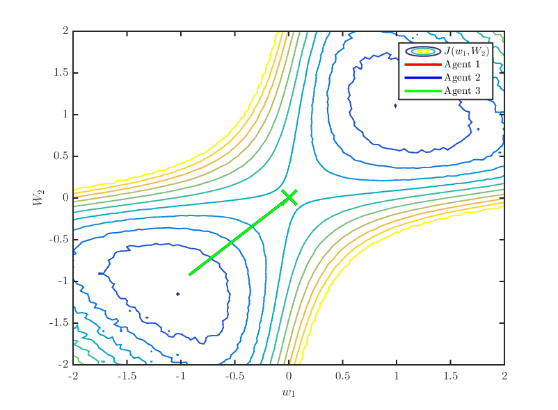
The cost surface is depicted in Fig. 2.

Refer to caption
Fig. 2: Cost surface of a simple neural network with ρ=0.1\rho=0.1.

It can be observed from the figure, and analytically verified, that J⁡(⋅)J(\cdot) has two local minima in the positive and negative quadrants, respectively, and a single saddle-point at w1=W2=0w_{1}=W_{2}=0. The Hessian matrix of J⁡(⋅)J(\cdot) at w1=W2=0w_{1}=W_{2}=0 evaluates to:

∇2J​(0,0)=(ρ−\E​𝜸′​𝒉2−\E​𝜸′​𝒉2ρ)\nabla^{2}J(0,0)=\begin{pmatrix}\rho&-\E\frac{\boldsymbol{\gamma}^{\prime}\boldsymbol{h}}{2}\\ -\E\frac{\boldsymbol{\gamma}^{\prime}\boldsymbol{h}}{2}&\rho\end{pmatrix} (66)

For this example, we let Pr{𝜸′=−1}=Pr{𝜸′=1}=12\mathrm{Pr}\left\{\boldsymbol{\gamma}^{\prime}=-1\right\}=\mathrm{Pr}\left\{\boldsymbol{\gamma}^{\prime}=1\right\}=\frac{1}{2} and 𝒉∼𝒩⁡(𝜸′,1)\boldsymbol{h}\sim\mathcal{N}\left(\boldsymbol{\gamma}^{\prime},1\right). Then, we obtain \E​𝜸′​\h=1\E\boldsymbol{\gamma}^{\prime}\h=1. We also let ρ=0.1\rho=0.1, so that:

∇2J​(0,0)=(0.1−0.5−0.50.1)\nabla^{2}J(0,0)=\begin{pmatrix}0.1&-0.5\\ -0.5&0.1\end{pmatrix} (67)

which has an eigenvalue at −0.4-0.4 with corresponding eigenvector col​{1,1}\mathrm{col}\left\{1,1\right\}. This implies that w1=W2=0w_{1}=W_{2}=0 is a strict saddle-point with local descent direction col​{1,1}\mathrm{col}\left\{1,1\right\}. It turns out, however that the gradient noise induced by the immediate stochastic gradient approximation ∇J^​(⋅)=∇Q​(⋅,𝜸′,𝒉)\widehat{\nabla J}(\cdot)=\nabla Q(\cdot;\boldsymbol{\gamma}^{\prime},\boldsymbol{h}) does not have a gradient noise component in the descent direction col​{1,1}\mathrm{col}\left\{1,1\right\} at the strict saddle-point w1=W2=0w_{1}=W_{2}=0. Indeed, note that with probability one we have ∇Q​(0,0,𝜸′,𝒉)=col⁡{0,0}=∇J​(0,0)\nabla Q(0,0;\boldsymbol{\gamma}^{\prime},\boldsymbol{h})=\mathrm{col}\{0,0\}=\nabla J(0,0) so that the gradient noise vanishes at w1=W2=0w_{1}=W_{2}=0. Hence, initializing all agents at w1=W2=0w_{1}=W_{2}=0 and iterating (2a)–(2b) would cause them to remain there with probability 11. This suggests that assumption 7 is not merely a technical condition but indeed necessary. To satisfy the assumption we construct the stochastic gradient approximation as:

∇J^​(w1,W2)≜∇Q​(w1,W2,𝜸′,\h)+𝒗⋅col⁡{1,1}\widehat{\nabla J}(w_{1},W_{2})\triangleq\nabla Q(w_{1},W_{2};\boldsymbol{\gamma}^{\prime},\h)+\boldsymbol{v}\cdot\mathrm{col}\left\{1,1\right\} (68)

where 𝒗∼𝒩⁡(0,1)\boldsymbol{v}\sim\mathcal{N}(0,1) acts only in the direction col​{1,1}\mathrm{col}\left\{1,1\right\} and ensures that gradient noise is present in the descent direction around the strict saddle-point at w1=W2=0w_{1}=W_{2}=0. Two realizations of the evolution are shown in Figures 3–4.

Refer to caption
Fig. 3: Agents are initialized at different points in space, but nevertheless quickly cluster. They then jointly travel away from the strict saddle-point and towards one of the local minimers.
Refer to caption
Fig. 4: Agents are initialized together precisely in the strict saddle-point. The presence of the gradient perturbation allows them to jointly escape the saddle-point.

Appendix A Proof of Lemma 1

Recall that

\si≜∑k=1Npk​\sk,i​(\wk,i−1)\displaystyle\s_{i}\triangleq\sum_{k=1}^{N}p_{k}\s_{k,i}\left(\w_{k,i-1}\right) (69)

and hence (48) holds. Using the smoothness assumption on the gradient noise term (46), we can write:

\E​{\si​\si\T|𝓕i−1}\displaystyle\>\E\left\{\s_{i}\s_{i}^{\T}|\boldsymbol{\mathcal{F}}_{i-1}\right\}
=\displaystyle= ∑k=1Npk2​Rs,k​(\wk,i−1)\displaystyle\>\sum_{k=1}^{N}p_{k}^{2}R_{s,k}\left(\w_{k,i-1}\right)
=\displaystyle= ∑k=1Npk2​Rs,k​(\wc,i−1)\displaystyle\>\sum_{k=1}^{N}p_{k}^{2}R_{s,k}\left(\w_{c,i-1}\right)
+(∑k=1Npk2​Rs,k​(\wk,i−1)−∑k=1Npk2​Rs,k​(\wc,i−1))\displaystyle\>+\left(\sum_{k=1}^{N}p_{k}^{2}R_{s,k}\left(\w_{k,i-1}\right)-\sum_{k=1}^{N}p_{k}^{2}R_{s,k}\left(\w_{c,i-1}\right)\right) (70)

so that:

‖ℛs​(𝟙⊗\wc,i−1)−ℛs​(𝟙⊗w)‖\displaystyle\>\left\|\mathcal{R}_{s}\left(\mathds{1}\otimes\w_{c,i-1}\right)-\mathcal{R}_{s}\left(\mathds{1}\otimes w\right)\right\|
=\displaystyle= ‖∑k=1Npk2​Rs,k​(\wc,i−1)−∑k=1Npk2​Rs,k​(w)‖\displaystyle\>\left\|\sum_{k=1}^{N}p_{k}^{2}R_{s,k}\left(\w_{c,i-1}\right)-\sum_{k=1}^{N}p_{k}^{2}R_{s,k}\left(w\right)\right\|
=\displaystyle= ‖∑k=1Npk2​(Rs,k​(\wc,i−1)−Rs,k​(w))‖\displaystyle\>\left\|\sum_{k=1}^{N}p_{k}^{2}\left(R_{s,k}\left(\w_{c,i-1}\right)-R_{s,k}\left(w\right)\right)\right\|
≤(a)\displaystyle\stackrel{{\scriptstyle(a)}}{{\leq}} ∑k=1Npk​‖pk​(Rs,k​(\wc,i−1)−Rs,k​(w))‖\displaystyle\>\sum_{k=1}^{N}p_{k}\left\|p_{k}\left(R_{s,k}\left(\w_{c,i-1}\right)-R_{s,k}\left(w\right)\right)\right\|
≤\displaystyle{\leq} pmax​∑k=1Npk​‖Rs,k​(\wc,i−1)−Rs,k​(w)‖\displaystyle\>p_{\max}\sum_{k=1}^{N}p_{k}\left\|R_{s,k}\left(\w_{c,i-1}\right)-R_{s,k}\left(w\right)\right\|
≤(b)\displaystyle\stackrel{{\scriptstyle(b)}}{{\leq}} pmax​βR​‖\wc,i−1−w‖γ\displaystyle\>p_{\max}\beta_{R}\left\|\w_{c,i-1}-w\right\|^{\gamma} (71)

where (a)(a) follows from Jensen’s inequality and (b)(b) follows from the Lipschitz condition on the gradient noise covariance (46) and ∑k=1Npk=1\sum_{k=1}^{N}p_{k}=1. Similarly:

‖Rs​(\bcwi−1)−Rs​(\bcwc,i−1)‖\displaystyle\>\left\|R_{s}\left(\bcw_{i-1}\right)-R_{s}\left(\bcw_{c,i-1}\right)\right\|
=\displaystyle= ‖∑k=1Npk2​Rs,k​(\wk,i−1)−∑k=1Npk2​Rs,k​(\wc,i−1)‖\displaystyle\>\left\|\sum_{k=1}^{N}p_{k}^{2}R_{s,k}\left(\w_{k,i-1}\right)-\sum_{k=1}^{N}p_{k}^{2}R_{s,k}\left(\w_{c,i-1}\right)\right\|
=\displaystyle= ‖∑k=1Npk2​(Rs,k​(\wk,i−1)−Rs,k​(\wc,i−1))‖\displaystyle\>\left\|\sum_{k=1}^{N}p_{k}^{2}\left(R_{s,k}\left(\w_{k,i-1}\right)-R_{s,k}\left(\w_{c,i-1}\right)\right)\right\|
≤\displaystyle\leq ∑k=1Npk​‖pk​(Rs,k​(\wk,i−1)−Rs,k​(\wc,i−1))‖\displaystyle\>\sum_{k=1}^{N}p_{k}\left\|p_{k}\left(R_{s,k}\left(\w_{k,i-1}\right)-R_{s,k}\left(\w_{c,i-1}\right)\right)\right\|
≤\displaystyle\leq pmax​βR​∑k=1Npk​‖\wk,i−1−\wc,i−1‖γ\displaystyle\>p_{\max}\beta_{R}\sum_{k=1}^{N}p_{k}\left\|\w_{k,i-1}-\w_{c,i-1}\right\|^{\gamma}
≤(a)\displaystyle\stackrel{{\scriptstyle(a)}}{{\leq}} pmax​βR​∑k=1Npk​‖\bcwi−1−\bcwc,i−1‖γ\displaystyle\>p_{\max}\beta_{R}\sum_{k=1}^{N}p_{k}\left\|\bcw_{i-1}-\bcw_{c,i-1}\right\|^{\gamma}
=\displaystyle= pmax​βR​‖\bcwi−1−\bcwc,i−1‖γ\displaystyle\>p_{\max}\beta_{R}\left\|\bcw_{i-1}-\bcw_{c,i-1}\right\|^{\gamma} (72)

where (a)(a) follows from the fact that xγx^{\gamma} is monotonically increasing in γ\gamma for x,γ>0x,\gamma>0 and:

‖\bcwi−1−\bcwc,i−1‖2=\displaystyle\left\|\bcw_{i-1}-\bcw_{c,i-1}\right\|^{2}= ∑k=1N‖\wk,i−1−\wc,i−1‖2\displaystyle\>\sum_{k=1}^{N}\left\|\w_{k,i-1}-\w_{c,i-1}\right\|^{2}
≥\displaystyle\geq ‖\wℓ,i−1−\wc,i−1‖2,∀ℓ\displaystyle\>\left\|\w_{\ell,i-1}-\w_{c,i-1}\right\|^{2},\ \ \forall\ \ell (73)

Appendix B Proof of Theorem 1

We shall carefully bound each of the terms appearing on the righthand side of (44), which we repeat here again for reference:

J⁡(\wc,i⋆+i′)≤\displaystyle J(\w_{c,i^{\star}+i}^{\prime})\leq J(\wc,i⋆)−∇J(\wc,i⋆)\T\w~i′i⋆\displaystyle\>J(\w_{c,i^{\star}})-{\nabla J(\w_{c,i^{\star}})}^{\T}\widetilde{\w}_{i}^{\prime}{}^{i^{\star}}
+12‖\w~i′‖i⋆∇2J​(\wc,i⋆)2+ρ6‖\w~i′‖i⋆3\displaystyle\>+\frac{1}{2}{\left\|\widetilde{\w}_{i}^{\prime}{}^{i^{\star}}\right\|}_{\nabla^{2}J(\w_{c,i^{\star}})}^{2}+\frac{\rho}{6}{\left\|\widetilde{\w}_{i}^{\prime}{}^{i^{\star}}\right\|}^{3} (74)

We begin by establishing a bound on the linear term in (74). Iterating the recursive relation for the short-term model (34) and taking expectations conditioned on 𝓕i⋆+i\boldsymbol{\mathcal{F}}_{i^{\star}+i} yields:

\E{\w~′|i+1i⋆𝓕i⋆+i}\displaystyle\>\E\left\{\widetilde{\w}^{\prime}{}^{i^{\star}}_{i+1}|\boldsymbol{\mathcal{F}}_{i^{\star}+i}\right\}
=\displaystyle= (I−μ∇2J(\wc,i⋆))\w~′ii⋆\displaystyle\>\left(I-\mu\nabla^{2}J(\w_{c,i^{\star}})\right)\widetilde{\w}^{\prime}{}^{i^{\star}}_{i}
+μ∇J(\wc,i⋆)+μ\E{\si⋆+i+1|𝓕i⋆+i}\displaystyle\>+\mu\nabla J(\w_{c,i^{\star}})+\mu\E\left\{\s_{i^{\star}+i+1}|\boldsymbol{\mathcal{F}}_{i^{\star}+i}\right\}
=\displaystyle= (I−μ∇2J(\wc,i⋆))\w~′+ii⋆μ∇J(\wc,i⋆)\displaystyle\>\left(I-\mu\nabla^{2}J(\w_{c,i^{\star}})\right)\widetilde{\w}^{\prime}{}^{i^{\star}}_{i}+\mu\nabla J(\w_{c,i^{\star}}) (75)

where the gradient-noise term disappeared in light of

\E​{\si⋆+i+1|𝓕i⋆+i}=0\E\left\{\s_{i^{\star}+i+1}|\boldsymbol{\mathcal{F}}_{i^{\star}+i}\right\}=0 (76)

by Assumption 4. Note that 𝓕i⋆+i\boldsymbol{\mathcal{F}}_{i^{\star}+i} denotes the information captured in \wk,j\w_{k,j} up to time i⋆+ii^{\star}+i, while 𝓕i⋆\boldsymbol{\mathcal{F}}_{i^{\star}} denotes the information available up to time i⋆i^{\star}. Hence:

𝓕i⋆+i=𝓕i⋆∪filtration⁡{\wk,i⋆+1,…,\wk,i⋆+i}\boldsymbol{\mathcal{F}}_{i^{\star}+i}=\boldsymbol{\mathcal{F}}_{i^{\star}}\cup\mathrm{filtration}\left\{\w_{k,i^{\star}+1},\ldots,\w_{k,i^{\star}+i}\right\} (77)

Hence, taking expectation of (75) conditioned on 𝓕i⋆\boldsymbol{\mathcal{F}}_{i^{\star}} removes the elements in filtration⁡{\wk,i⋆+1,…,\wk,i⋆+i}\mathrm{filtration}\left\{\w_{k,i^{\star}+1},\ldots,\w_{k,i^{\star}+i}\right\} contained in 𝓕i⋆\boldsymbol{\mathcal{F}}_{i^{\star}} and yields:

\E{\w~′|i+1i⋆𝓕i⋆}=\displaystyle\E\left\{\widetilde{\w}^{\prime}{}^{i^{\star}}_{i+1}|\boldsymbol{\mathcal{F}}_{i^{\star}}\right\}= (I−μ∇2J(\wc,i⋆))\E{\w~′|ii⋆𝓕i⋆}\displaystyle\>\left(I-\mu\nabla^{2}J(\w_{c,i^{\star}})\right)\E\left\{\widetilde{\w}^{\prime}{}^{i^{\star}}_{i}|\boldsymbol{\mathcal{F}}_{i^{\star}}\right\}
+μ∇J(\wc,i⋆)\displaystyle\>+\mu\nabla J(\w_{c,i^{\star}}) (78)

Since \w~′i⋆0=0\widetilde{\w}^{\prime}{}^{i^{\star}}_{0}=0, iterating starting at i=0i=0 yields:

\E{\w~′|ii⋆𝓕i⋆}=μ(∑k=1i(I−μ∇2J(\wc,i⋆))k−1)∇J(\wc,i⋆)\E\left\{\widetilde{\w}^{\prime}{}^{i^{\star}}_{i}|\boldsymbol{\mathcal{F}}_{i^{\star}}\right\}=\mu\left(\sum_{k=1}^{i}{\left(I-\mu\nabla^{2}J(\w_{c,i^{\star}})\right)}^{k-1}\right)\nabla J(\w_{c,i^{\star}}) (79)

This allows us to bound the linear term appearing in (74) as:

−\E{∇J(\wc,i⋆)\T\w~i′|i⋆𝓕i⋆}\displaystyle\>-\E\left\{{\nabla J(\w_{c,i^{\star}})}^{\T}\widetilde{\w}_{i}^{\prime}{}^{i^{\star}}|\boldsymbol{\mathcal{F}}_{i^{\star}}\right\}
=\displaystyle= −∇J(\wc,i⋆)\T\E{\w~i′|i⋆𝓕i⋆}\displaystyle\>-{\nabla J(\w_{c,i^{\star}})}^{\T}\E\left\{\widetilde{\w}_{i}^{\prime}{}^{i^{\star}}|\boldsymbol{\mathcal{F}}_{i^{\star}}\right\}
=(79)\displaystyle\stackrel{{\scriptstyle\eqref{eq:mean_deviation_saddle}}}{{=}} −μ∇J(\wc,i⋆)\T(∑k=1i(I−μ∇2J(\wc,i⋆))k−1)∇J(\wc,i⋆)\displaystyle\>-\mu{\nabla J(\w_{c,i^{\star}})}^{\T}\left(\sum_{k=1}^{i}{\left(I-\mu\nabla^{2}J(\w_{c,i^{\star}})\right)}^{k-1}\right)\nabla J(\w_{c,i^{\star}})
=\displaystyle= −μ​‖∇J​(\wc,i⋆)‖∑k=1i(I−μ​∇2J​(\wc,i⋆))k−12\displaystyle\>-\mu{\left\|\nabla J(\w_{c,i^{\star}})\right\|}^{2}_{\sum_{k=1}^{i}{\left(I-\mu\nabla^{2}J(\w_{c,i^{\star}})\right)}^{k-1}} (80)

We now examine the quadratic term in (74). To this end, we introduce the eigenvalue decomposition of the Hessian around the iterate at time i⋆i^{\star}:

∇2J​(\wc,i⋆)≜𝑽i⋆​𝚲i⋆​𝑽i⋆\T\nabla^{2}J(\w_{c,i^{\star}})\triangleq\boldsymbol{V}_{i^{\star}}\boldsymbol{\Lambda}_{i^{\star}}\boldsymbol{V}_{i^{\star}}^{\T} (81)

Note that both 𝑽i⋆\boldsymbol{V}_{i^{\star}} and 𝚲i⋆\boldsymbol{\Lambda}_{i^{\star}} inherit their randomness from \wc,i⋆\w_{c,i^{\star}}. As such, they are random but become deterministic when conditioning on 𝓕i⋆\boldsymbol{\mathcal{F}}_{i^{\star}}. This fact will be exploited further below. To begin with, note that:

‖\w~′‖i+1i⋆∇2J​(\wc,i⋆)2=\displaystyle{\left\|\widetilde{\w}^{\prime}{}^{i^{\star}}_{i+1}\right\|}_{\nabla^{2}J(\w_{c,i^{\star}})}^{2}= ‖\w~′‖i+1i⋆𝑽i⋆​𝚲i⋆​𝑽i⋆\T2\displaystyle\>{\left\|\widetilde{\w}^{\prime}{}^{i^{\star}}_{i+1}\right\|}_{\boldsymbol{V}_{i^{\star}}\boldsymbol{\Lambda}_{i^{\star}}\boldsymbol{V}_{i^{\star}}^{\T}}^{2}
=\displaystyle= ‖𝑽i⋆\T​\wc,i⋆−𝑽i⋆\T​\wc,i⋆+i+1′‖𝚲i⋆2\displaystyle\>{\left\|\boldsymbol{V}_{i^{\star}}^{\T}{\w}_{c,i^{\star}}-\boldsymbol{V}_{i^{\star}}^{\T}{\w}_{c,i^{\star}+i+1}^{\prime}\right\|}_{\boldsymbol{\Lambda}_{i^{\star}}}^{2}
=\displaystyle= ‖\w¯′‖i+1i⋆𝚲i⋆2\displaystyle\>{\left\|\overline{\w}^{\prime}{}^{i^{\star}}_{i+1}\right\|}_{\boldsymbol{\Lambda}_{i^{\star}}}^{2} (82)

where we introducted:

\w¯′i⋆i+1≜𝑽i⋆\T\w~′i⋆i+1\displaystyle\overline{\w}^{\prime}{}^{i^{\star}}_{i+1}\triangleq\boldsymbol{V}_{i^{\star}}^{\T}\widetilde{\w}^{\prime}{}^{i^{\star}}_{i+1} (83)

Under this transformation, recursion (34) is also diagonalized, yielding:

\w¯′i⋆i+1\displaystyle\>\overline{\w}^{\prime}{}^{i^{\star}}_{i+1}
≜\displaystyle\triangleq 𝑽i⋆\T\w~′i⋆i+1\displaystyle\>\boldsymbol{V}_{i^{\star}}^{\T}\widetilde{\w}^{\prime}{}^{i^{\star}}_{i+1}
=\displaystyle= 𝑽i⋆\T(I−μ∇2J(\wc,i⋆))𝑽i⋆𝑽i⋆\T\w~′ii⋆\displaystyle\>\boldsymbol{V}_{i^{\star}}^{\T}\left(I-\mu\nabla^{2}J(\w_{c,i^{\star}})\right)\boldsymbol{V}_{i^{\star}}\boldsymbol{V}_{i^{\star}}^{\T}\widetilde{\w}^{\prime}{}^{i^{\star}}_{i}
+μ𝑽i⋆\T∇J(\wc,i⋆)+μ𝑽i⋆\T\si⋆+i+1\displaystyle\>+\mu\boldsymbol{V}_{i^{\star}}^{\T}{\nabla}J(\w_{c,i^{\star}})+\mu\boldsymbol{V}_{i^{\star}}^{\T}\s_{i^{\star}+i+1}
=\displaystyle= (I−μ𝚲i⋆)\w¯′+ii⋆μ∇¯J(\wc,i⋆)+μ\s¯i⋆+i+1\displaystyle\>\left(I-\mu\boldsymbol{\Lambda}_{i^{\star}}\right)\overline{\w}^{\prime}{}^{i^{\star}}_{i}+\mu\overline{\nabla}J(\w_{c,i^{\star}})+\mu\overline{\s}_{i^{\star}+i+1} (84)

with ∇¯J(\wc,i⋆)≜𝑽i⋆\T∇J(\wc,i⋆)\overline{\nabla}J(\w_{c,i^{\star}})\triangleq\boldsymbol{V}_{i^{\star}}^{\T}{\nabla}J(\w_{c,i^{\star}}) and \s¯i⋆+i+1≜𝑽i⋆\T​\si⋆+i+1\overline{\s}_{i^{\star}+i+1}\triangleq\boldsymbol{V}_{i^{\star}}^{\T}\s_{i^{\star}+i+1}. The presence of the gradient term, which is deterministic conditioned on 𝓕i⋆\boldsymbol{\mathcal{F}}_{i^{\star}} complicates the analysis of the evolution. It can be removed by (conditionally) centering the random variable. Specifically, applying the same tranformation to the conditional mean recursion (78), and subtracting the transformed conditional mean on both sides of (84), we find:

\w¯′−i+1i⋆\E{\w¯′|i+1i⋆𝓕i⋆}\displaystyle\>\overline{\w}^{\prime}{}^{i^{\star}}_{i+1}-\E\left\{\overline{\w}^{\prime}{}^{i^{\star}}_{i+1}|\boldsymbol{\mathcal{F}}_{i^{\star}}\right\}
=\displaystyle= (I−μ𝚲i⋆)(\w¯′−ii⋆\E{\w¯′|ii⋆𝓕i⋆})+μ\s¯i⋆+i+1\displaystyle\>\left(I-\mu\boldsymbol{\Lambda}_{i^{\star}}\right)\left(\overline{\w}^{\prime}{}^{i^{\star}}_{i}-\E\left\{\overline{\w}^{\prime}{}^{i^{\star}}_{i}|\boldsymbol{\mathcal{F}}_{i^{\star}}\right\}\right)+\mu\overline{\s}_{i^{\star}+i+1} (85)

which allows us to cancel the driving term involving the gradient. For brevity, define the (conditionally) centered random variable:

\wˇ′=i+1i⋆\w¯′−i+1i⋆\E{\w¯′|i+1i⋆𝓕i⋆}\check{\w}^{\prime}{}^{i^{\star}}_{i+1}=\overline{\w}^{\prime}{}^{i^{\star}}_{i+1}-\E\left\{\overline{\w}^{\prime}{}^{i^{\star}}_{i+1}|\boldsymbol{\mathcal{F}}_{i^{\star}}\right\} (86)

so that:

\wˇ′=i+1i⋆(I−μ𝚲i⋆)\wˇ′+ii⋆μ\s¯i⋆+i+1\displaystyle\check{\w}^{\prime}{}^{i^{\star}}_{i+1}=\left(I-\mu\boldsymbol{\Lambda}_{i^{\star}}\right)\check{\w}^{\prime}{}^{i^{\star}}_{i}+\mu\overline{\s}_{i^{\star}+i+1} (87)

Before proceeding, note that we can express:

\E{‖\wˇ′‖ii⋆𝚲i⋆2|𝓕i⋆}\displaystyle\>\E\left\{{\left\|\check{\w}^{\prime}{}^{i^{\star}}_{i}\right\|}_{\boldsymbol{\Lambda}_{i^{\star}}}^{2}|\boldsymbol{\mathcal{F}}_{i^{\star}}\right\}
=\displaystyle= \E{‖\w¯′−ii⋆\E{\w¯′|ii⋆𝓕i⋆}‖𝚲i⋆2|𝓕i⋆}\displaystyle\>\E\left\{{\left\|\overline{\w}^{\prime}{}^{i^{\star}}_{i}-\E\left\{\overline{\w}^{\prime}{}^{i^{\star}}_{i}|\boldsymbol{\mathcal{F}}_{i^{\star}}\right\}\right\|}_{\boldsymbol{\Lambda}_{i^{\star}}}^{2}|\boldsymbol{\mathcal{F}}_{i^{\star}}\right\}
=\displaystyle= \E{‖\w¯′‖ii⋆𝚲i⋆2|𝓕i⋆}−‖\E{\w¯′|ii⋆𝓕i⋆}‖𝚲i⋆2\displaystyle\>\E\left\{{\left\|\overline{\w}^{\prime}{}^{i^{\star}}_{i}\right\|}_{\boldsymbol{\Lambda}_{i^{\star}}}^{2}|\boldsymbol{\mathcal{F}}_{i^{\star}}\right\}-{\left\|\E\left\{\overline{\w}^{\prime}{}^{i^{\star}}_{i}|\boldsymbol{\mathcal{F}}_{i^{\star}}\right\}\right\|}_{\boldsymbol{\Lambda}_{i^{\star}}}^{2} (88)

Hence, we have:

\E{‖\w~′‖ii⋆∇2J​(\wc,i⋆)2|𝓕i⋆}\displaystyle\>\E\left\{{\left\|\widetilde{\w}^{\prime}{}^{i^{\star}}_{i}\right\|}_{\nabla^{2}J(\w_{c,i^{\star}})}^{2}|\boldsymbol{\mathcal{F}}_{i^{\star}}\right\}
=\displaystyle= \E{‖\w¯′‖ii⋆𝚲i⋆2|𝓕i⋆}\displaystyle\>\E\left\{{\left\|\overline{\w}^{\prime}{}^{i^{\star}}_{i}\right\|}_{\boldsymbol{\Lambda}_{i^{\star}}}^{2}|\boldsymbol{\mathcal{F}}_{i^{\star}}\right\}
=\displaystyle= \E{‖\wˇ′‖ii⋆𝚲i⋆2|𝓕i⋆}+‖\E{\w¯′|ii⋆𝓕i⋆}‖𝚲i⋆2\displaystyle\>\E\left\{{\left\|\check{\w}^{\prime}{}^{i^{\star}}_{i}\right\|}_{\boldsymbol{\Lambda}_{i^{\star}}}^{2}|\boldsymbol{\mathcal{F}}_{i^{\star}}\right\}+{\left\|\E\left\{\overline{\w}^{\prime}{}^{i^{\star}}_{i}|\boldsymbol{\mathcal{F}}_{i^{\star}}\right\}\right\|}_{\boldsymbol{\Lambda}_{i^{\star}}}^{2} (89)

In order to make claims about \E{‖\w~′‖ii⋆∇2J​(\wc,i⋆)2|𝓕i⋆}\E\left\{{\left\|\widetilde{\w}^{\prime}{}^{i^{\star}}_{i}\right\|}_{\nabla^{2}J(\w_{c,i^{\star}})}^{2}|\boldsymbol{\mathcal{F}}_{i^{\star}}\right\} by studying \E{‖\wˇ′‖ii⋆𝚲i⋆2|𝓕i⋆}\E\left\{{\left\|\check{\w}^{\prime}{}^{i^{\star}}_{i}\right\|}_{\boldsymbol{\Lambda}_{i^{\star}}}^{2}|\boldsymbol{\mathcal{F}}_{i^{\star}}\right\}, we need to establish a bound on ‖\E{\w¯′|ii⋆𝓕i⋆}‖𝚲i⋆2{\left\|\E\left\{\overline{\w}^{\prime}{}^{i^{\star}}_{i}|\boldsymbol{\mathcal{F}}_{i^{\star}}\right\}\right\|}_{\boldsymbol{\Lambda}_{i^{\star}}}^{2}. We have:

‖\E{\w¯′|ii⋆𝓕i⋆}‖𝚲i⋆2\displaystyle\>{\left\|\E\left\{\overline{\w}^{\prime}{}^{i^{\star}}_{i}|\boldsymbol{\mathcal{F}}_{i^{\star}}\right\}\right\|}_{\boldsymbol{\Lambda}_{i^{\star}}}^{2}
=\displaystyle= ‖\E{𝑽i⋆\T\w~′|ii⋆𝓕i⋆}‖𝚲i⋆2\displaystyle\>{\left\|\E\left\{\boldsymbol{V}_{i^{\star}}^{\T}\widetilde{\w}^{\prime}{}^{i^{\star}}_{i}|\boldsymbol{\mathcal{F}}_{i^{\star}}\right\}\right\|}_{\boldsymbol{\Lambda}_{i^{\star}}}^{2}
=(79)\displaystyle\stackrel{{\scriptstyle\eqref{eq:mean_deviation_saddle}}}{{=}} μ2‖𝑽i⋆\T(∑k=1i(I−μ∇2J(\wc,i⋆))k−1)∇J(\wc,i⋆)‖𝚲i⋆2\displaystyle\>\mu^{2}{\left\|\boldsymbol{V}_{i^{\star}}^{\T}\left(\sum_{k=1}^{i}{\left(I-\mu\nabla^{2}J(\w_{c,i^{\star}})\right)}^{k-1}\right)\nabla J(\w_{c,i^{\star}})\right\|}_{\boldsymbol{\Lambda}_{i^{\star}}}^{2}
=\displaystyle= μ2​‖(∑k=1i(I−μ​𝚲i⋆)k−1)​∇¯​J​(\wc,i⋆)‖𝚲i⋆2\displaystyle\>\mu^{2}{\left\|\left(\sum_{k=1}^{i}{\left(I-\mu\boldsymbol{\Lambda}_{i^{\star}}\right)}^{k-1}\right)\overline{\nabla}J(\w_{c,i^{\star}})\right\|}_{\boldsymbol{\Lambda}_{i^{\star}}}^{2}
=\displaystyle= μ2​∇¯​J​(\wc,i⋆)\T​(∑k=1i(I−μ​𝚲i⋆)k−1)​𝚲i⋆\displaystyle\>\mu^{2}{\overline{\nabla}J(\w_{c,i^{\star}})}^{\T}\left(\sum_{k=1}^{i}{\left(I-\mu\boldsymbol{\Lambda}_{i^{\star}}\right)}^{k-1}\right)\boldsymbol{\Lambda}_{i^{\star}}
×(∑k=1i(I−μ​𝚲i⋆)k−1)​∇¯​J​(\wc,i⋆)\displaystyle\>\ \ \ \ \times\left(\sum_{k=1}^{i}{\left(I-\mu\boldsymbol{\Lambda}_{i^{\star}}\right)}^{k-1}\right)\overline{\nabla}J(\w_{c,i^{\star}}) (90)

We shall order the eigenvalues of ∇2J​(\wc,i⋆)\nabla^{2}J(\w_{c,i^{\star}}), such that its eigendecomposition has a block structure:

𝑽i⋆=[𝑽i⋆≥0𝑽i⋆<0],𝚲i⋆=[𝚲i⋆≥000𝚲i⋆<0]\boldsymbol{V}_{i^{\star}}=\left[\begin{array}[]{cc}\boldsymbol{V}_{i^{\star}}^{\geq 0}&\boldsymbol{V}_{i^{\star}}^{<0}\end{array}\right],\ \ \boldsymbol{\Lambda}_{i^{\star}}=\left[\begin{array}[]{cc}\boldsymbol{\Lambda}_{i^{\star}}^{\geq 0}&0\\ 0&\boldsymbol{\Lambda}_{i^{\star}}^{<0}\end{array}\right] (91)

with δ​I≥𝚲i⋆≥0≥0\delta I\geq\boldsymbol{\Lambda}_{i^{\star}}^{\geq 0}\geq 0 and 𝚲i⋆<0<0\boldsymbol{\Lambda}_{i^{\star}}^{<0}<0. Note that since ∇2J​(\wc,i⋆)\nabla^{2}J(\w_{c,i^{\star}}) is random, the decomposition itself is random as well. Nevertheless, it exists with probability one. We also decompose the transformed gradient vector with appropriate dimesions:

∇¯​J​(\wc,i⋆)=col⁡{∇¯​J​(\wc,i⋆)≥0,∇¯​J​(\wc,i⋆)<0}{\overline{\nabla}J(\w_{c,i^{\star}})}=\mathrm{col}\left\{{\overline{\nabla}J(\w_{c,i^{\star}})}^{\geq 0},{\overline{\nabla}J(\w_{c,i^{\star}})}^{<0}\right\} (92)

We can then decompose (90):

‖\E{\w¯′|ii⋆𝓕i⋆}‖𝚲i⋆2\displaystyle\>{\left\|\E\left\{\overline{\w}^{\prime}{}^{i^{\star}}_{i}|\boldsymbol{\mathcal{F}}_{i^{\star}}\right\}\right\|}_{\boldsymbol{\Lambda}_{i^{\star}}}^{2}
=\displaystyle{=} μ2​∇¯​J​(\wc,i⋆)\T​(∑k=1i(I−μ​𝚲i⋆)k−1)​𝚲i⋆\displaystyle\>\mu^{2}{\overline{\nabla}J(\w_{c,i^{\star}})}^{\T}\left(\sum_{k=1}^{i}{\left(I-\mu\boldsymbol{\Lambda}_{i^{\star}}\right)}^{k-1}\right)\boldsymbol{\Lambda}_{i^{\star}}
×(∑k=1i(I−μ​𝚲i⋆)k−1)​∇¯​J​(\wc,i⋆)\displaystyle\>\ \ \ \ \times\left(\sum_{k=1}^{i}{\left(I-\mu\boldsymbol{\Lambda}_{i^{\star}}\right)}^{k-1}\right)\overline{\nabla}J(\w_{c,i^{\star}})
=\displaystyle= μ2​(∇¯​J​(\wc,i⋆)≥0)\T​(∑k=1i(I−μ​𝚲i⋆≥0)k−1)​𝚲i⋆≥0\displaystyle\>\mu^{2}{\left({\overline{\nabla}J(\w_{c,i^{\star}})}^{\geq 0}\right)}^{\T}\left(\sum_{k=1}^{i}{\left(I-\mu\boldsymbol{\Lambda}_{i^{\star}}^{\geq 0}\right)}^{k-1}\right)\boldsymbol{\Lambda}_{i^{\star}}^{\geq 0}
×(∑k=1i(I−μ​𝚲i⋆≥0)k−1)​∇¯​J​(\wc,i⋆)≥0\displaystyle\>\ \ \ \ \times\left(\sum_{k=1}^{i}{\left(I-\mu\boldsymbol{\Lambda}_{i^{\star}}^{\geq 0}\right)}^{k-1}\right)\overline{\nabla}J(\w_{c,i^{\star}})^{\geq 0}
+μ2​(∇¯​J​(\wc,i⋆)<0)\T​(∑k=1i(I−μ​𝚲i⋆<0)k−1)​𝚲i⋆<0\displaystyle\>+\mu^{2}{\left({\overline{\nabla}J(\w_{c,i^{\star}})}^{<0}\right)}^{\T}\left(\sum_{k=1}^{i}{\left(I-\mu\boldsymbol{\Lambda}_{i^{\star}}^{<0}\right)}^{k-1}\right)\boldsymbol{\Lambda}_{i^{\star}}^{<0}
×(∑k=1i(I−μ​𝚲i⋆<0)k−1)​∇¯​J​(\wc,i⋆)<0\displaystyle\>\ \ \ \ \times\left(\sum_{k=1}^{i}{\left(I-\mu\boldsymbol{\Lambda}_{i^{\star}}^{<0}\right)}^{k-1}\right)\overline{\nabla}J(\w_{c,i^{\star}})^{<0}
≤(a)\displaystyle\stackrel{{\scriptstyle(a)}}{{\leq}} μ2​(∇¯​J​(\wc,i⋆)≥0)\T​(∑k=1i(I−μ​𝚲i⋆≥0)k−1)​𝚲i⋆≥0\displaystyle\>\mu^{2}{\left({\overline{\nabla}J(\w_{c,i^{\star}})}^{\geq 0}\right)}^{\T}\left(\sum_{k=1}^{i}{\left(I-\mu\boldsymbol{\Lambda}_{i^{\star}}^{\geq 0}\right)}^{k-1}\right)\boldsymbol{\Lambda}_{i^{\star}}^{\geq 0}
×(∑k=1i(I−μ​𝚲i⋆≥0)k−1)​∇¯​J​(\wc,i⋆)≥0\displaystyle\>\ \ \ \ \times\left(\sum_{k=1}^{i}{\left(I-\mu\boldsymbol{\Lambda}_{i^{\star}}^{\geq 0}\right)}^{k-1}\right)\overline{\nabla}J(\w_{c,i^{\star}})^{\geq 0}
≤(b)\displaystyle\stackrel{{\scriptstyle(b)}}{{\leq}} μ2​(∇¯​J​(\wc,i⋆)≥0)\T​(∑k=1∞(I−μ​𝚲i⋆≥0)k−1)​𝚲i⋆≥0\displaystyle\>\mu^{2}{\left({\overline{\nabla}J(\w_{c,i^{\star}})}^{\geq 0}\right)}^{\T}\left(\sum_{k=1}^{\infty}{\left(I-\mu\boldsymbol{\Lambda}_{i^{\star}}^{\geq 0}\right)}^{k-1}\right)\boldsymbol{\Lambda}_{i^{\star}}^{\geq 0}
×(∑k=1i(I−μ​𝚲i⋆≥0)k−1)​∇¯​J​(\wc,i⋆)≥0\displaystyle\>\ \ \ \ \times\left(\sum_{k=1}^{i}{\left(I-\mu\boldsymbol{\Lambda}_{i^{\star}}^{\geq 0}\right)}^{k-1}\right)\overline{\nabla}J(\w_{c,i^{\star}})^{\geq 0}
=(c)\displaystyle\stackrel{{\scriptstyle(c)}}{{=}} μ2​(∇¯​J​(\wc,i⋆)≥0)\T​(μ​𝚲i⋆≥0)−1​𝚲i⋆≥0\displaystyle\>\mu^{2}{\left({\overline{\nabla}J(\w_{c,i^{\star}})}^{\geq 0}\right)}^{\T}\left(\mu\boldsymbol{\Lambda}_{i^{\star}}^{\geq 0}\right)^{-1}\boldsymbol{\Lambda}_{i^{\star}}^{\geq 0}
×(∑k=1i(I−μ​𝚲i⋆≥0)k−1)​∇¯​J​(\wc,i⋆)≥0\displaystyle\>\ \ \ \ \times\left(\sum_{k=1}^{i}{\left(I-\mu\boldsymbol{\Lambda}_{i^{\star}}^{\geq 0}\right)}^{k-1}\right)\overline{\nabla}J(\w_{c,i^{\star}})^{\geq 0}
=\displaystyle{=} μ​(∇¯​J​(\wc,i⋆)≥0)\T​(∑k=1i(I−μ​𝚲i⋆≥0)k−1)​∇¯​J​(\wc,i⋆)≥0\displaystyle\>\mu{\left({\overline{\nabla}J(\w_{c,i^{\star}})}^{\geq 0}\right)}^{\T}\left(\sum_{k=1}^{i}{\left(I-\mu\boldsymbol{\Lambda}_{i^{\star}}^{\geq 0}\right)}^{k-1}\right)\overline{\nabla}J(\w_{c,i^{\star}})^{\geq 0}
≤(d)\displaystyle\stackrel{{\scriptstyle(d)}}{{\leq}} μ​(∇¯​J​(\wc,i⋆)≥0)\T​(∑k=1i(I−μ​𝚲i⋆≥0)k−1)​∇¯​J​(\wc,i⋆)≥0\displaystyle\>\mu{\left({\overline{\nabla}J(\w_{c,i^{\star}})}^{\geq 0}\right)}^{\T}\left(\sum_{k=1}^{i}{\left(I-\mu\boldsymbol{\Lambda}_{i^{\star}}^{\geq 0}\right)}^{k-1}\right)\overline{\nabla}J(\w_{c,i^{\star}})^{\geq 0}
+μ​(∇¯​J​(\wc,i⋆)<0)\T​(∑k=1i(I−μ​𝚲i⋆<0)k−1)​∇¯​J​(\wc,i⋆)<0\displaystyle\>+\mu{\left({\overline{\nabla}J(\w_{c,i^{\star}})}^{<0}\right)}^{\T}\left(\sum_{k=1}^{i}{\left(I-\mu\boldsymbol{\Lambda}_{i^{\star}}^{<0}\right)}^{k-1}\right)\overline{\nabla}J(\w_{c,i^{\star}})^{<0}
≤\displaystyle{\leq} μ​∇¯​J​(\wc,i⋆)\T​(∑k=1i(I−μ​𝚲i⋆)k−1)​∇¯​J​(\wc,i⋆)\displaystyle\>\mu{{\overline{\nabla}J(\w_{c,i^{\star}})}}^{\T}\left(\sum_{k=1}^{i}{\left(I-\mu\boldsymbol{\Lambda}_{i^{\star}}\right)}^{k-1}\right)\overline{\nabla}J(\w_{c,i^{\star}})
=\displaystyle{=} μ​‖∇¯​J​(\wc,i⋆)‖∑k=1i(I−μ​𝚲i⋆)k−12\displaystyle\>\mu{\left\|{\overline{\nabla}J(\w_{c,i^{\star}})}\right\|}^{2}_{\sum_{k=1}^{i}{\left(I-\mu\boldsymbol{\Lambda}_{i^{\star}}\right)}^{k-1}} (93)

where (a)(a) follows from 𝚲i⋆<0<0\boldsymbol{\Lambda}_{i^{\star}}^{<0}<0, (b)(b) follows from:

∑k=1k(I−μ​𝚲i⋆≥0)k−1≤∑k=1∞(I−μ​𝚲i⋆≥0)k−1\sum_{k=1}^{k}{\left(I-\mu\boldsymbol{\Lambda}_{i^{\star}}^{\geq 0}\right)}^{k-1}\leq\sum_{k=1}^{\infty}{\left(I-\mu\boldsymbol{\Lambda}_{i^{\star}}^{\geq 0}\right)}^{k-1} (94)

for μ<1δ\mu<\frac{1}{\delta}. Step (c)(c) follows from the formula for the geometric matrix series, and (d)(d) follows from:

μ​(∇¯​J​(\wc,i⋆)≥0)\T​(∑k=1i(I−μ​𝚲i⋆≥0)k−1)​∇¯​J​(\wc,i⋆)≥0≥0\mu{\left({\overline{\nabla}J(\w_{c,i^{\star}})}^{\geq 0}\right)}^{\T}\left(\sum_{k=1}^{i}{\left(I-\mu\boldsymbol{\Lambda}_{i^{\star}}^{\geq 0}\right)}^{k-1}\right)\overline{\nabla}J(\w_{c,i^{\star}})^{\geq 0}\geq 0 (95)

Comparing (93) to (80), we find that we can bound:

−\E{∇J(\wc,i⋆)\T\w~i′|i⋆𝓕i⋆}+‖\E{\w¯′|ii⋆𝓕i⋆}‖𝚲i⋆2≤0\displaystyle-\E\left\{{\nabla J(\w_{c,i^{\star}})}^{\T}\widetilde{\w}_{i}^{\prime}{}^{i^{\star}}|\boldsymbol{\mathcal{F}}_{i^{\star}}\right\}+{\left\|\E\left\{\overline{\w}^{\prime}{}^{i^{\star}}_{i}|\boldsymbol{\mathcal{F}}_{i^{\star}}\right\}\right\|}_{\boldsymbol{\Lambda}_{i^{\star}}}^{2}\leq 0 (96)

To recap, we can simplify (74) as:

\E​{J⁡(\wc,i⋆+i′)|𝓕i⋆}\displaystyle\>\E\left\{J(\w_{c,i^{\star}+i}^{\prime})|\boldsymbol{\mathcal{F}}_{i^{\star}}\right\}
≤\displaystyle\leq J(\wc,i⋆)+12\E{‖\wˇ′‖ii⋆𝚲i⋆2|𝓕i⋆}+ρ6\E{‖\w~i′‖i⋆3|𝓕i⋆}\displaystyle\>J(\w_{c,i^{\star}})+\frac{1}{2}\E\left\{{\left\|\check{\w}^{\prime}{}^{i^{\star}}_{i}\right\|}_{\boldsymbol{\Lambda}_{i^{\star}}}^{2}|\boldsymbol{\mathcal{F}}_{i^{\star}}\right\}+\frac{\rho}{6}\E\left\{{\left\|\widetilde{\w}_{i}^{\prime}{}^{i^{\star}}\right\|}^{3}|\boldsymbol{\mathcal{F}}_{i^{\star}}\right\} (97)

We proceed with the now simplified quadratic term. We square both sides of (87) under an arbitrary diagonal weighting matrix 𝚺i\boldsymbol{\Sigma}_{i}, deterministic conditioned on \wc,i⋆\w_{c,i^{\star}} and \wc,i⋆+i\w_{c,i^{\star}+i}, to obtain:

‖\wˇ′‖i+1i⋆𝚺i2\displaystyle{\left\|\check{\w}^{\prime}{}^{i^{\star}}_{i+1}\right\|}_{\boldsymbol{\Sigma}_{i}}^{2}
=\displaystyle= ‖(I−μ𝚲i⋆)\wˇ′+ii⋆μ\s¯i⋆+i+1‖𝚺i2\displaystyle\>{\left\|\left(I-\mu\boldsymbol{\Lambda}_{i^{\star}}\right)\check{\w}^{\prime}{}^{i^{\star}}_{i}+\mu\overline{\s}_{i^{\star}+i+1}\right\|}_{\boldsymbol{\Sigma}_{i}}^{2}
=\displaystyle= ‖(I−μ𝚲i⋆)\wˇ′‖ii⋆𝚺i2+μ2‖\s¯i⋆+i+1‖𝚺i2\displaystyle\>{\left\|\left(I-\mu\boldsymbol{\Lambda}_{i^{\star}}\right)\check{\w}^{\prime}{}^{i^{\star}}_{i}\right\|}_{\boldsymbol{\Sigma}_{i}}^{2}+\mu^{2}{\left\|\overline{\s}_{i^{\star}+i+1}\right\|}_{\boldsymbol{\Sigma}_{i}}^{2}
+2μ\wˇ′\Tii⋆(I−μ𝚲i⋆)𝚺i\s¯i⋆+i+1\displaystyle+2\mu{\check{\w}^{\prime}{}^{i^{\star}}_{i}}^{\T}\left(I-\mu\boldsymbol{\Lambda}_{i^{\star}}\right)\boldsymbol{\Sigma}_{i}\overline{\s}_{i^{\star}+i+1} (98)

Note that upon conditioning on 𝓕i⋆+i\boldsymbol{\mathcal{F}}_{i^{\star}+i}, all elements of the cross-term, aside from \s¯i⋆+i+1\overline{\s}_{i^{\star}+i+1}, become deterministic, and as such the term disappears when taking expecations. We obtain:

\E{‖\wˇ′‖i+1i⋆𝚺i2|𝓕i⋆+i}\displaystyle\>\E\left\{{\left\|\check{\w}^{\prime}{}^{i^{\star}}_{i+1}\right\|}_{\boldsymbol{\Sigma}_{i}}^{2}|\boldsymbol{\mathcal{F}}_{i^{\star}+i}\right\}
=\displaystyle= ‖(I−μ𝚲i⋆)\wˇ′‖ii⋆𝚺i2+μ2\E{‖\s¯i⋆+i+1‖𝚺i2|𝓕i⋆+i}\displaystyle\>{\left\|\left(I-\mu\boldsymbol{\Lambda}_{i^{\star}}\right)\check{\w}^{\prime}{}^{i^{\star}}_{i}\right\|}_{\boldsymbol{\Sigma}_{i}}^{2}+\mu^{2}\E\left\{{\left\|\overline{\s}_{i^{\star}+i+1}\right\|}_{\boldsymbol{\Sigma}_{i}}^{2}|\boldsymbol{\mathcal{F}}_{i^{\star}+i}\right\}
=\displaystyle= ‖\wˇ′‖ii⋆𝚺i−2​μ​𝚲i⋆​𝚺i+μ2​𝚲i⋆​𝚺i​𝚲i⋆2\displaystyle\>{\left\|\check{\w}^{\prime}{}^{i^{\star}}_{i}\right\|}_{\boldsymbol{\Sigma}_{i}-2\mu\boldsymbol{\Lambda}_{i^{\star}}\boldsymbol{\Sigma}_{i}+\mu^{2}\boldsymbol{\Lambda}_{i^{\star}}\boldsymbol{\Sigma}_{i}\boldsymbol{\Lambda}_{i^{\star}}}^{2}
+μ2​Tr​(𝑽i⋆​𝚺i​𝑽i⋆\T​ℛs​(\bcwi⋆+i))\displaystyle\>+\mu^{2}\mathrm{Tr}\left(\boldsymbol{V}_{i^{\star}}\boldsymbol{\Sigma}_{i}\boldsymbol{V}_{i^{\star}}^{\T}\mathcal{R}_{s}\left(\bcw_{i^{\star}+i}\right)\right)
=\displaystyle= ‖\wˇ′‖ii⋆𝚺i−2​μ​𝚲i⋆​𝚺i2+μ2Tr(𝑽i⋆𝚺i𝑽i⋆\Tℛs(\bcwc,i⋆))\displaystyle\>{\left\|\check{\w}^{\prime}{}^{i^{\star}}_{i}\right\|}_{\boldsymbol{\Sigma}_{i}-2\mu\boldsymbol{\Lambda}_{i^{\star}}\boldsymbol{\Sigma}_{i}}^{2}+\mu^{2}\mathrm{Tr}\left(\boldsymbol{V}_{i^{\star}}\boldsymbol{\Sigma}_{i}\boldsymbol{V}_{i^{\star}}^{\T}\mathcal{R}_{s}\left(\bcw_{c,i^{\star}}\right)\right)
+μ2​Tr​(𝑽i⋆​𝚺i​𝑽i⋆\T​(ℛs​(\bcwi⋆+i)−ℛs​(\bcwc,i⋆)))\displaystyle\>+\mu^{2}\mathrm{Tr}\left(\boldsymbol{V}_{i^{\star}}\boldsymbol{\Sigma}_{i}\boldsymbol{V}_{i^{\star}}^{\T}\left(\mathcal{R}_{s}\left(\bcw_{i^{\star}+i}\right)-\mathcal{R}_{s}\left(\bcw_{c,i^{\star}}\right)\right)\right)
+μ2‖\wˇ′‖ii⋆𝚲i⋆​𝚺i​𝚲i⋆2\displaystyle\>+\mu^{2}{\left\|\check{\w}^{\prime}{}^{i^{\star}}_{i}\right\|}_{\boldsymbol{\Lambda}_{i^{\star}}\boldsymbol{\Sigma}_{i}\boldsymbol{\Lambda}_{i^{\star}}}^{2} (99)

We proceed to bound the last two terms. First, we have:

Tr⁡(𝑽i⋆​𝚺i​𝑽i⋆\T​(ℛs​(\bcwi⋆+i)−ℛs​(\bcwc,i⋆)))\displaystyle\>\mathrm{Tr}\left(\boldsymbol{V}_{i^{\star}}\boldsymbol{\Sigma}_{i}\boldsymbol{V}_{i^{\star}}^{\T}\left(\mathcal{R}_{s}\left(\bcw_{i^{\star}+i}\right)-\mathcal{R}_{s}\left(\bcw_{c,i^{\star}}\right)\right)\right)
≤(a)\displaystyle\overset{(a)}{\leq} ‖𝑽i⋆​𝚺i​𝑽i⋆\T‖​‖ℛs​(\bcwi⋆+i)−ℛs​(\bcwc,i⋆)‖\displaystyle\>\left\|\boldsymbol{V}_{i^{\star}}\boldsymbol{\Sigma}_{i}\boldsymbol{V}_{i^{\star}}^{\T}\right\|\left\|\mathcal{R}_{s}\left(\bcw_{i^{\star}+i}\right)-\mathcal{R}_{s}\left(\bcw_{c,i^{\star}}\right)\right\|
≤\displaystyle{\leq} ‖𝑽i⋆​𝚺i​𝑽i⋆\T‖|ℛs​(\bcwi⋆+i)−ℛs​(\bcwc,i⋆+i)\displaystyle\>\left\|\boldsymbol{V}_{i^{\star}}\boldsymbol{\Sigma}_{i}\boldsymbol{V}_{i^{\star}}^{\T}\right\|\|\mathcal{R}_{s}\left(\bcw_{i^{\star}+i}\right)-\mathcal{R}_{s}\left(\bcw_{c,i^{\star}+i}\right)
+ℛs(\bcwc,i⋆+i)−ℛs(\bcwc,i⋆)∥\displaystyle\>\ \ \ \ \ \ \ \ \ \ \ \ \ \ \ \ \ +\mathcal{R}_{s}\left(\bcw_{c,i^{\star}+i}\right)-\mathcal{R}_{s}\left(\bcw_{c,i^{\star}}\right)\|
≤\displaystyle{\leq} ‖𝑽i⋆​𝚺i​𝑽i⋆\T‖​‖ℛs​(\bcwi⋆+i)−ℛs​(\bcwc,i⋆+i)‖\displaystyle\>\left\|\boldsymbol{V}_{i^{\star}}\boldsymbol{\Sigma}_{i}\boldsymbol{V}_{i^{\star}}^{\T}\right\|\left\|\mathcal{R}_{s}\left(\bcw_{i^{\star}+i}\right)-\mathcal{R}_{s}\left(\bcw_{c,i^{\star}+i}\right)\right\|
+‖𝑽i⋆​𝚺i​𝑽i⋆\T‖​‖ℛs​(\bcwc,i⋆+i)−ℛs​(\bcwc,i⋆)‖\displaystyle\>+\left\|\boldsymbol{V}_{i^{\star}}\boldsymbol{\Sigma}_{i}\boldsymbol{V}_{i^{\star}}^{\T}\right\|\left\|\mathcal{R}_{s}\left(\bcw_{c,i^{\star}+i}\right)-\mathcal{R}_{s}\left(\bcw_{c,i^{\star}}\right)\right\|
≤(b)\displaystyle\overset{(b)}{\leq} ρ⁡(𝚺i)​βR​pmax​(‖\wc,i⋆+i−\wc,i⋆‖γ+‖\bcwc,i⋆+i−\bcwi⋆+i‖γ)\displaystyle\>\rho\left(\boldsymbol{\Sigma}_{i}\right)\beta_{R}p_{\max}\left({\left\|\w_{c,i^{\star}+i}-\w_{c,i^{\star}}\right\|}^{\gamma}+{\left\|\bcw_{c,i^{\star}+i}-\bcw_{i^{\star}+i}\right\|}^{\gamma}\right)
=\displaystyle{=} ρ⁡(𝚺i)​βR​pmax​(‖\w~ii⋆‖γ+‖\bcwc,i⋆+i−\bcwi⋆+i‖γ)\displaystyle\>\rho\left(\boldsymbol{\Sigma}_{i}\right)\beta_{R}p_{\max}\left({\left\|\widetilde{\w}^{{i}^{\star}}_{i}\right\|}^{\gamma}+\left\|\bcw_{c,i^{\star}+i}-\bcw_{i^{\star}+i}\right\|^{\gamma}\right) (100)

where (a)(a) follows from Cauchy-Schwarz, since Tr⁡(A\T​B)\mathrm{Tr}(A^{\T}B) is an inner product over the space of symmetric matricess, and hence, |Tr⁡(A\T​B)|≤‖A‖​‖B‖|\mathrm{Tr}(A^{\T}B)|\leq\|A\|\|B\|, and (b)(b) follows from Lemma (1). For the second term, we have:

‖\wˇ′‖ii⋆𝚲i⋆​𝚺i​𝚲i⋆2\displaystyle{\left\|\check{\w}^{\prime}{}^{i^{\star}}_{i}\right\|}_{\boldsymbol{\Lambda}_{i^{\star}}\boldsymbol{\Sigma}_{i}\boldsymbol{\Lambda}_{i^{\star}}}^{2} ≤ρ(𝚲i⋆𝚺i𝚲i⋆)‖\wˇ′‖ii⋆2\displaystyle\leq\rho\left(\boldsymbol{\Lambda}_{i^{\star}}\boldsymbol{\Sigma}_{i}\boldsymbol{\Lambda}_{i^{\star}}\right){\left\|\check{\w}^{\prime}{}^{i^{\star}}_{i}\right\|}^{2}
≤δ2ρ(𝚺i)‖\wˇ′‖ii⋆2\displaystyle\leq\delta^{2}\rho\left(\boldsymbol{\Sigma}_{i}\right){\left\|\check{\w}^{\prime}{}^{i^{\star}}_{i}\right\|}^{2} (101)

We conclude that

\E{‖\wˇ′‖i+1i⋆𝚺i2|𝓕i⋆}\displaystyle\>\E\left\{{\left\|\check{\w}^{\prime}{}^{i^{\star}}_{i+1}\right\|}_{\boldsymbol{\Sigma}_{i}}^{2}|\boldsymbol{\mathcal{F}}_{i^{\star}}\right\}
=\displaystyle= \E{‖\wˇ′‖ii⋆𝚺i−2​μ​𝚲i⋆​𝚺i2|𝓕i⋆}\displaystyle\>\E\left\{{\left\|\check{\w}^{\prime}{}^{i^{\star}}_{i}\right\|}_{\boldsymbol{\Sigma}_{i}-2\mu\boldsymbol{\Lambda}_{i^{\star}}\boldsymbol{\Sigma}_{i}}^{2}|\boldsymbol{\mathcal{F}}_{i^{\star}}\right\}
+μ2​Tr​(𝑽i⋆​𝚺i​𝑽i⋆\T​ℛs​(\bcwc,i⋆))+μ2​ρ​(𝚺i)​\E​{𝒒i⋆+i|𝓕i⋆}\displaystyle\>+\mu^{2}\mathrm{Tr}\left(\boldsymbol{V}_{i^{\star}}\boldsymbol{\Sigma}_{i}\boldsymbol{V}_{i^{\star}}^{\T}\mathcal{R}_{s}\left(\bcw_{c,i^{\star}}\right)\right)+\mu^{2}\rho\left(\boldsymbol{\Sigma}_{i}\right)\E\left\{\boldsymbol{q}_{i^{\star}+i}|\boldsymbol{\mathcal{F}}_{i^{\star}}\right\} (102)

where

𝒒i⋆+i≜βRpmax(‖\w~ii⋆‖γ+‖\bcwc,i⋆+i−\bcwi⋆+i‖γ)+δ2‖\wˇ′‖ii⋆2\displaystyle\boldsymbol{q}_{i^{\star}+i}\triangleq\beta_{R}p_{\max}\left({\left\|\widetilde{\w}^{{i}^{\star}}_{i}\right\|}^{\gamma}+\left\|\bcw_{c,i^{\star}+i}-\bcw_{i^{\star}+i}\right\|^{\gamma}\right)+\delta^{2}{\left\|\check{\w}^{\prime}{}^{i^{\star}}_{i}\right\|}^{2} (103)

For brevity, we define

𝑫\displaystyle\boldsymbol{D} ≜I−2​μ​𝚲i⋆\displaystyle\triangleq I-2\mu\boldsymbol{\Lambda}_{i^{\star}} (104)
𝒀\displaystyle\boldsymbol{Y} ≜𝑽i⋆\T​ℛs​(\bcwc,i⋆)​𝑽i⋆\displaystyle\triangleq\boldsymbol{V}_{i^{\star}}^{\T}\mathcal{R}_{s}\left(\bcw_{c,i^{\star}}\right)\boldsymbol{V}_{i^{\star}} (105)

With these substitutions we obtain:

\E{‖\wˇ′‖i+1i⋆𝚺i2|𝓕i⋆}\displaystyle\>\E\left\{{\left\|\check{\w}^{\prime}{}^{i^{\star}}_{i+1}\right\|}_{\boldsymbol{\Sigma}_{i}}^{2}|\boldsymbol{\mathcal{F}}_{i^{\star}}\right\}
=\displaystyle= \E{‖\wˇ′‖ii⋆𝑫​𝚺i2|𝓕i⋆}+μ2Tr(𝚺i𝒀)\displaystyle\>\E\left\{{\left\|\check{\w}^{\prime}{}^{i^{\star}}_{i}\right\|}_{\boldsymbol{D}\boldsymbol{\Sigma}_{i}}^{2}|\boldsymbol{\mathcal{F}}_{i^{\star}}\right\}+\mu^{2}\mathrm{Tr}\left(\boldsymbol{\Sigma}_{i}\boldsymbol{Y}\right)
+μ2​ρ​(𝚺i)​\E​{𝒒i⋆+i|𝓕i⋆}\displaystyle\>+\mu^{2}\rho\left(\boldsymbol{\Sigma}_{i}\right)\E\left\{\boldsymbol{q}_{i^{\star}+i}|\boldsymbol{\mathcal{F}}_{i^{\star}}\right\} (106)

At i=0i=0, we have:

\wˇ′=0i⋆\w¯′−0i⋆\E{\w¯′|0i⋆𝓕i⋆}=0−0=0\check{\w}^{\prime}{}^{i^{\star}}_{0}=\overline{\w}^{\prime}{}^{i^{\star}}_{0}-\E\left\{\overline{\w}^{\prime}{}^{i^{\star}}_{0}|\boldsymbol{\mathcal{F}}_{i^{\star}}\right\}=0-0=0 (107)

Letting 𝚺i=𝚲i⋆​𝑫i\boldsymbol{\Sigma}_{i}=\boldsymbol{\Lambda}_{i^{\star}}\boldsymbol{D}^{i}, we can iterate to obtain:

\E{‖\wˇ′‖i+1i⋆𝚲i⋆2|𝓕i⋆}\displaystyle\>\E\left\{{\left\|\check{\w}^{\prime}{}^{i^{\star}}_{i+1}\right\|}_{\boldsymbol{\Lambda}_{i^{\star}}}^{2}|\boldsymbol{\mathcal{F}}_{i^{\star}}\right\}
=\displaystyle= μ2​∑n=0iTr⁡(𝚲i⋆​𝑫n​𝒀)\displaystyle\>\mu^{2}\sum_{n=0}^{i}\mathrm{Tr}\left(\boldsymbol{\Lambda}_{i^{\star}}\boldsymbol{D}^{n}\boldsymbol{Y}\right)
+μ2∑n=0iρ(𝚲i⋆𝑫n)⋅\E{𝒒i⋆+n|𝓕i⋆}\displaystyle\>+\mu^{2}\sum_{n=0}^{i}\rho\left(\boldsymbol{\Lambda}_{i^{\star}}\boldsymbol{D}^{n}\right)\cdot\E\left\{\boldsymbol{q}_{i^{\star}+n}|\boldsymbol{\mathcal{F}}_{i^{\star}}\right\}
=\displaystyle= μ2​Tr​(𝚲i⋆​(∑n=0i𝑫n)​𝒀)\displaystyle\>\mu^{2}\mathrm{Tr}\left(\boldsymbol{\Lambda}_{i^{\star}}\left(\sum_{n=0}^{i}\boldsymbol{D}^{n}\right)\boldsymbol{Y}\right)
+μ2∑n=0iρ(𝚲i⋆𝑫n)⋅\E{𝒒i⋆+n|𝓕i⋆}\displaystyle\>+\mu^{2}\sum_{n=0}^{i}\rho\left(\boldsymbol{\Lambda}_{i^{\star}}\boldsymbol{D}^{n}\right)\cdot\E\left\{\boldsymbol{q}_{i^{\star}+n}|\boldsymbol{\mathcal{F}}_{i^{\star}}\right\} (108)

since \w¯c,i⋆+i+1′=\w¯c,i⋆\overline{\w}_{c,i^{\star}+i+1}^{\prime}=\overline{\w}_{c,i^{\star}} at i=0i=0. Our objective is to show that the first term on the right-hand side yields sufficient descent (i.e., will be sufficiently negative), while the second term is small enough to be negligible. To this end, we again make use of the structured eigendecomposition (91). We have:

μ2​Tr​(𝚲i⋆​(∑n=0i𝑫n)​𝑽i⋆\T​ℛs​(\bcwc,i⋆)​𝑽i⋆)\displaystyle\>\mu^{2}\mathrm{Tr}\left(\boldsymbol{\Lambda}_{i^{\star}}\left(\sum_{n=0}^{i}\boldsymbol{D}^{n}\right)\boldsymbol{V}_{i^{\star}}^{\T}\mathcal{R}_{s}\left(\bcw_{c,i^{\star}}\right)\boldsymbol{V}_{i^{\star}}\right)
=(a)\displaystyle\stackrel{{\scriptstyle(a)}}{{=}} μ2​Tr​(𝚲i⋆≥0​(∑n=0i(I−2​μ​𝚲i⋆≥0)n)CLOSE\displaystyle\>\mu^{2}\mathrm{Tr}\Bigg(\boldsymbol{\Lambda}_{i^{\star}}^{\geq 0}\left(\sum_{n=0}^{i}{\left(I-2\mu\boldsymbol{\Lambda}_{i^{\star}}^{\geq 0}\right)}^{n}\right)
×(𝑽i⋆≥0)\Tℛs(\bcwc,i⋆)𝑽i⋆≥0)\displaystyle\>\ \ \ \ \ \ \ \ \times{\left(\boldsymbol{V}_{i^{\star}}^{\geq 0}\right)}^{\T}\mathcal{R}_{s}\left(\bcw_{c,i^{\star}}\right)\boldsymbol{V}_{i^{\star}}^{\geq 0}\Bigg)
+μ2​Tr​(𝚲i⋆<0​(∑n=0i(I−2​μ​𝚲i⋆<0)n)CLOSE\displaystyle\>+\mu^{2}\mathrm{Tr}\Bigg(\boldsymbol{\Lambda}_{i^{\star}}^{<0}\left(\sum_{n=0}^{i}{\left(I-2\mu\boldsymbol{\Lambda}_{i^{\star}}^{<0}\right)}^{n}\right)
×(𝑽i⋆<0)\Tℛs(\bcwc,i⋆)𝑽i⋆<0)\displaystyle\>\ \ \ \ \ \ \ \ \ \ \ \ \times{\left(\boldsymbol{V}_{i^{\star}}^{<0}\right)}^{\T}\mathcal{R}_{s}\left(\bcw_{c,i^{\star}}\right)\boldsymbol{V}_{i^{\star}}^{<0}\Bigg)
=(b)\displaystyle\stackrel{{\scriptstyle(b)}}{{=}} μ2​Tr​(𝚲i⋆≥0​(∑n=0i(I−2​μ​𝚲i⋆≥0)n)CLOSE\displaystyle\>\mu^{2}\mathrm{Tr}\Bigg(\boldsymbol{\Lambda}_{i^{\star}}^{\geq 0}\left(\sum_{n=0}^{i}{\left(I-2\mu\boldsymbol{\Lambda}_{i^{\star}}^{\geq 0}\right)}^{n}\right)
×(𝑽i⋆≥0)\Tℛs(\bcwc,i⋆)𝑽i⋆≥0)\displaystyle\>\ \ \ \ \ \ \ \ \times{\left(\boldsymbol{V}_{i^{\star}}^{\geq 0}\right)}^{\T}\mathcal{R}_{s}\left(\bcw_{c,i^{\star}}\right)\boldsymbol{V}_{i^{\star}}^{\geq 0}\Bigg)
−μ2​Tr​((−𝚲i⋆<0)​(∑n=0i(I−2​μ​𝚲i⋆<0)n)CLOSE\displaystyle\>-\mu^{2}\mathrm{Tr}\Bigg(\left(-\boldsymbol{\Lambda}_{i^{\star}}^{<0}\right)\left(\sum_{n=0}^{i}{\left(I-2\mu\boldsymbol{\Lambda}_{i^{\star}}^{<0}\right)}^{n}\right)
×(𝑽i⋆<0)\Tℛs(\bcwc,i⋆)𝑽i⋆<0)\displaystyle\>\ \ \ \ \ \ \ \ \ \ \ \times{\left(\boldsymbol{V}_{i^{\star}}^{<0}\right)}^{\T}\mathcal{R}_{s}\left(\bcw_{c,i^{\star}}\right)\boldsymbol{V}_{i^{\star}}^{<0}\Bigg)
≤(c)\displaystyle\stackrel{{\scriptstyle(c)}}{{\leq}} μ2​Tr​(𝚲i⋆≥0​(∑n=0i(I−2​μ​𝚲i⋆≥0)n))\displaystyle\>\mu^{2}\mathrm{Tr}\left(\boldsymbol{\Lambda}_{i^{\star}}^{\geq 0}\left(\sum_{n=0}^{i}{\left(I-2\mu\boldsymbol{\Lambda}_{i^{\star}}^{\geq 0}\right)}^{n}\right)\right)
×λmax​((𝑽i⋆≥0)\T​ℛs​(\bcwc,i⋆)​𝑽i⋆≥0)\displaystyle\>\times\lambda_{\max}\left({\left(\boldsymbol{V}_{i^{\star}}^{\geq 0}\right)}^{\T}\mathcal{R}_{s}\left(\bcw_{c,i^{\star}}\right)\boldsymbol{V}_{i^{\star}}^{\geq 0}\right)
−μ2​Tr​((−𝚲i⋆<0)​(∑n=0i(I−2​μ​𝚲i⋆<0)n))\displaystyle\>-\mu^{2}\mathrm{Tr}\left(\left(-\boldsymbol{\Lambda}_{i^{\star}}^{<0}\right)\left(\sum_{n=0}^{i}{\left(I-2\mu\boldsymbol{\Lambda}_{i^{\star}}^{<0}\right)}^{n}\right)\right)
×λmin​((𝑽i⋆<0)\T​ℛs​(\bcwc,i⋆)​𝑽i⋆<0)\displaystyle\>\times\lambda_{\min}\left({\left(\boldsymbol{V}_{i^{\star}}^{<0}\right)}^{\T}\mathcal{R}_{s}\left(\bcw_{c,i^{\star}}\right)\boldsymbol{V}_{i^{\star}}^{<0}\right)
≤(d)\displaystyle\stackrel{{\scriptstyle(d)}}{{\leq}} μ2​Tr​(𝚲i⋆≥0​(∑n=0i(I−2​μ​𝚲i⋆≥0)n))​σu2\displaystyle\>\mu^{2}\mathrm{Tr}\left(\boldsymbol{\Lambda}_{i^{\star}}^{\geq 0}\left(\sum_{n=0}^{i}{\left(I-2\mu\boldsymbol{\Lambda}_{i^{\star}}^{\geq 0}\right)}^{n}\right)\right)\sigma_{u}^{2}
−μ2​Tr​((−𝚲i⋆<0)​(∑n=0i(I−2​μ​𝚲i⋆<0)n))​σℓ2\displaystyle\>-\mu^{2}\mathrm{Tr}\left(\left(-\boldsymbol{\Lambda}_{i^{\star}}^{<0}\right)\left(\sum_{n=0}^{i}{\left(I-2\mu\boldsymbol{\Lambda}_{i^{\star}}^{<0}\right)}^{n}\right)\right)\sigma_{\ell}^{2} (109)

where in (a)(a) we decomposed the trace since 𝚲i⋆​(∑n=0i𝑫n)\boldsymbol{\Lambda}_{i^{\star}}\left(\sum_{n=0}^{i}\boldsymbol{D}^{n}\right) is a diagonal matrix, (b)(b) applies −(−𝚲i⋆<0)=𝚲i⋆<0-\left(-\boldsymbol{\Lambda}_{i^{\star}}^{<0}\right)=\boldsymbol{\Lambda}_{i^{\star}}^{<0}. Step (b)(b) follows from Tr⁡(A)​λmin​(B)≤Tr⁡(A​B)≤Tr⁡(A)​λmax​(B)\mathrm{Tr}(A)\lambda_{\min}(B)\leq\mathrm{Tr}(AB)\leq\mathrm{Tr}(A)\lambda_{\max}(B) which holds for A=A\T,B=B\T≥0A=A^{\T},B=B^{\T}\geq 0, and (c)(c) follows from the bounded covariance property (51) and Assumption 7. For the positive term, we have:

μ2​Tr​(𝚲i⋆≥0​(∑n=0i(I−2​μ​𝚲i⋆≥0)n))​σu2\displaystyle\>\mu^{2}\mathrm{Tr}\left(\boldsymbol{\Lambda}_{i^{\star}}^{\geq 0}\left(\sum_{n=0}^{i}{\left(I-2\mu\boldsymbol{\Lambda}_{i^{\star}}^{\geq 0}\right)}^{n}\right)\right)\sigma_{u}^{2}
≤(a)\displaystyle\stackrel{{\scriptstyle(a)}}{{\leq}} μ2​Tr​(𝚲i⋆≥0​(∑n=0∞(I−2​μ​𝚲i⋆≥0)n))​σu2\displaystyle\>\mu^{2}\mathrm{Tr}\left(\boldsymbol{\Lambda}_{i^{\star}}^{\geq 0}\left(\sum_{n=0}^{\infty}{\left(I-2\mu\boldsymbol{\Lambda}_{i^{\star}}^{\geq 0}\right)}^{n}\right)\right)\sigma_{u}^{2}
≤(b)\displaystyle\stackrel{{\scriptstyle(b)}}{{\leq}} μ2​Tr​(𝚲i⋆≥0​(2​μ​𝚲i⋆≥0)−1)​σu2≤(c)μ2​M​σu2\displaystyle\>\mu^{2}\mathrm{Tr}\left(\boldsymbol{\Lambda}_{i^{\star}}^{\geq 0}{\left(2\mu\boldsymbol{\Lambda}_{i^{\star}}^{\geq 0}\right)}^{-1}\right)\sigma_{u}^{2}\stackrel{{\scriptstyle(c)}}{{\leq}}\>\frac{\mu}{2}M\sigma_{u}^{2} (110)

where (a)(a) follows since I−2​μ​𝚲i⋆≥0I-2\mu\boldsymbol{\Lambda}_{i^{\star}}^{\geq 0} is elementwise non-negative for μ≤2δ\mu\leq\frac{2}{\delta}, (b)(b) follows from ∑n=0∞An=(I−A)−1\sum_{n=0}^{\infty}A^{n}={\left(I-A\right)}^{-1} and (c)(c) follows since ∇2J​(\wc,i⋆)\nabla^{2}J(\w_{c,i^{\star}}) is of dimension MM.

For the negative term, we have under expectation conditioned on \wc,i⋆∈ℋ\w_{c,i^{\star}}\in\mathcal{H}:

\E​{Tr⁡((−𝚲i⋆<0)​(∑n=0i(I−2​μ​𝚲i⋆<0)n))​σℓ2|\wc,i⋆∈ℋ}\displaystyle\>\E\Bigg\{\mathrm{Tr}\left(\left(-\boldsymbol{\Lambda}_{i^{\star}}^{<0}\right)\left(\sum_{n=0}^{i}{\left(I-2\mu\boldsymbol{\Lambda}_{i^{\star}}^{<0}\right)}^{n}\right)\right)\sigma_{\ell}^{2}\Bigg|\w_{c,i^{\star}}\in\mathcal{H}\Bigg\}
≥(a)\displaystyle\stackrel{{\scriptstyle(a)}}{{\geq}} \E​{τ⁡(∑n=0i(1+2​μ​τ)n)​σℓ2|\wc,i⋆∈ℋ}\displaystyle\>\E\left\{\tau\left(\sum_{n=0}^{i}{\left(1+2\mu\tau\right)}^{n}\right)\sigma_{\ell}^{2}\Bigg|\w_{c,i^{\star}}\in\mathcal{H}\right\}
=(b)\displaystyle\stackrel{{\scriptstyle(b)}}{{=}} τ⁡(∑n=0i(1+2​μ​τ)n)​σℓ2=(c)τ​1−(1+2​μ​τ)i+11−(1+2​μ​τ)​σℓ2\displaystyle\>\tau\left(\sum_{n=0}^{i}{\left(1+2\mu\tau\right)}^{n}\right)\sigma_{\ell}^{2}\stackrel{{\scriptstyle(c)}}{{=}}\>\tau\frac{1-{\left(1+2\mu\tau\right)}^{i+1}}{1-(1+2\mu\tau)}\sigma_{\ell}^{2}
=\displaystyle{=} 12​μ​((1+2​μ​τ)i+1−1)​σℓ2\displaystyle\>\frac{1}{2\mu}\left({\left(1+2\mu\tau\right)}^{i+1}-1\right)\sigma_{\ell}^{2} (111)

Step (a)(a) makes use of the fact that (−𝚲i⋆<0)​(∑n=0i(I−2​μ​𝚲i⋆<0)n)\left(-\boldsymbol{\Lambda}_{i^{\star}}^{<0}\right)\left(\sum_{n=0}^{i}{\left(I-2\mu\boldsymbol{\Lambda}_{i^{\star}}^{<0}\right)}^{n}\right) is a diagonal matrix, where all elements are non-negative. Hence, its trace can be bounded by any of its diagonal elements:

Tr⁡((−𝚲i⋆<0)​(∑n=0i(I−2​μ​𝚲i⋆<0)n))\displaystyle\>\mathrm{Tr}\left(\left(-\boldsymbol{\Lambda}_{i^{\star}}^{<0}\right)\left(\sum_{n=0}^{i}{\left(I-2\mu\boldsymbol{\Lambda}_{i^{\star}}^{<0}\right)}^{n}\right)\right)
≥(17)\displaystyle\stackrel{{\scriptstyle\eqref{eq:define_h}}}{{\geq}} τ⁡(∑n=0i(1+2​μ​τ)n)\displaystyle\>\tau\left(\sum_{n=0}^{i}{\left(1+2\mu\tau\right)}^{n}\right) (112)

In (b)(b) we dropped the expectation since the expression is no longer random, and (c)(c) is the result of a geometric series. We return to the full expression (109) and find:

μ2\E{Tr(𝚲i⋆(∑n=0i𝑫n)\displaystyle\>\mu^{2}\E\Bigg\{\mathrm{Tr}\Bigg(\boldsymbol{\Lambda}_{i^{\star}}\left(\sum_{n=0}^{i}\boldsymbol{D}^{n}\right)
×𝑽i⋆\Tℛs(\bcwc,i⋆)𝑽i⋆)|\wc,i⋆∈ℋ}\displaystyle\>\ \ \ \ \ \ \ \ \ \ \ \ \ \ \times\boldsymbol{V}_{i^{\star}}^{\T}\mathcal{R}_{s}\left(\bcw_{c,i^{\star}}\right)\boldsymbol{V}_{i^{\star}}\Bigg)|\w_{c,i^{\star}}\in\mathcal{H}\Bigg\}
≤\displaystyle\leq μ2​M​σu2−μ2​((1+2​μ​τ)i+1−1)​σℓ2≤(a)−μ2​M​σu2\displaystyle\>\frac{\mu}{2}M\sigma_{u}^{2}-\frac{\mu}{2}\left({\left(1+2\mu\tau\right)}^{i+1}-1\right)\sigma_{\ell}^{2}\stackrel{{\scriptstyle(a)}}{{\leq}}\>-\frac{\mu}{2}M\sigma_{u}^{2} (113)

where (a)(a) holds if, and only if,

μ2​M​σu2−μ2​((1+2​μ​τ)i+1−1)​σℓ2≤−μ2​M​σu2\displaystyle\frac{\mu}{2}M\sigma_{u}^{2}-\frac{\mu}{2}\left({\left(1+2\mu\tau\right)}^{i+1}-1\right)\sigma_{\ell}^{2}\leq-\frac{\mu}{2}M\sigma_{u}^{2}
⟺\displaystyle\Longleftrightarrow\> 2​M​σu2σℓ2+1≤(1+2​μ​τ)i+1\displaystyle 2M\frac{\sigma_{u}^{2}}{\sigma_{\ell}^{2}}+1\leq{\left(1+2\mu\tau\right)}^{i+1}
⟺\displaystyle\Longleftrightarrow\> log⁡(2​M​σu2σℓ2+1)≤(i+1)​log⁡(1+2​μ​τ)\displaystyle\log\left(2M\frac{\sigma_{u}^{2}}{\sigma_{\ell}^{2}}+1\right)\leq(i+1){\log{\left(1+2\mu\tau\right)}}
⟺\displaystyle\Longleftrightarrow\> log⁡(2​M​σu2σℓ2+1)log⁡(1+2​μ​τ)≤i+1\displaystyle\frac{\log\left(2M\frac{\sigma_{u}^{2}}{\sigma_{\ell}^{2}}+1\right)}{\log{\left(1+2\mu\tau\right)}}\leq{i+1}
⟺\displaystyle\Longleftrightarrow\> log⁡(2​M​σu2σℓ2+1)O⁡(μ​τ)≤i+1\displaystyle\frac{\log\left(2M\frac{\sigma_{u}^{2}}{\sigma_{\ell}^{2}}+1\right)}{O(\mu\tau)}\leq{i+1} (114)

where the last line follows from limx→01/x​log⁡(1+x)=1\lim_{x\to 0}1/x\log(1+x)=1. We conclude that there exists a bounded isi^{s} such that:

μ2​\E​{Tr⁡(𝚲i⋆​(∑n=0is𝑫n)​𝑽i⋆\T​ℛs​(\bcwc,i⋆)​𝑽i⋆)}\displaystyle\>\mu^{2}\E\left\{\mathrm{Tr}\left(\boldsymbol{\Lambda}_{i^{\star}}\left(\sum_{n=0}^{i^{s}}\boldsymbol{D}^{n}\right)\boldsymbol{V}_{i^{\star}}^{\T}\mathcal{R}_{s}\left(\bcw_{c,i^{\star}}\right)\boldsymbol{V}_{i^{\star}}\right)\right\}
≤\displaystyle\leq −μ2​M​σu2\displaystyle\>-\frac{\mu}{2}M\sigma_{u}^{2} (115)

Applying this relation to (108) and taking expectations over \wc,i⋆∈ℋ\w_{c,i^{\star}}\in\mathcal{H}, we obtain:

\E{‖\wˇ′‖is+1i⋆𝚲i⋆2|\wc,i⋆∈ℋ}\displaystyle\>\E\left\{{\left\|\check{\w}^{\prime}{}^{i^{\star}}_{i^{s}+1}\right\|}_{\boldsymbol{\Lambda}_{i^{\star}}}^{2}|\w_{c,i^{\star}}\in\mathcal{H}\right\}
≤\displaystyle\leq μ2​∑n=0is\E​{(Tr⁡(𝚲i⋆​𝑫n)⋅\E​{𝒒i⋆+n|𝓕i⋆})|\wc,i⋆∈ℋ}\displaystyle\>\mu^{2}\sum_{n=0}^{i^{s}}\E\left\{\left(\mathrm{Tr}\left(\boldsymbol{\Lambda}_{i^{\star}}\boldsymbol{D}^{n}\right)\cdot\E\left\{\boldsymbol{q}_{i^{\star}+n}|\boldsymbol{\mathcal{F}}_{i^{\star}}\right\}\right)|\w_{c,i^{\star}}\in\mathcal{H}\right\}
−μ2​M​σu2\displaystyle\>-\frac{\mu}{2}M\sigma_{u}^{2} (116)

We now bound the perturbation term:

μ2​∑n=0is\E​{(ρ⁡(𝚲i⋆​𝑫n)⋅\E​{𝒒i⋆+n|𝓕i⋆})|\wc,i⋆∈ℋ}\displaystyle\>\mu^{2}\sum_{n=0}^{i^{s}}\E\left\{\left(\rho\left(\boldsymbol{\Lambda}_{i^{\star}}\boldsymbol{D}^{n}\right)\cdot\E\left\{\boldsymbol{q}_{i^{\star}+n}|\boldsymbol{\mathcal{F}}_{i^{\star}}\right\}\right)|\w_{c,i^{\star}}\in\mathcal{H}\right\}
≤\displaystyle\leq μ2​∑n=0is\E​{(ρ⁡(δ​I​(I+2​μ​δ​I)n)⋅\E​{𝒒i⋆+n|𝓕i⋆})|\wc,i⋆∈ℋ}\displaystyle\>\mu^{2}\sum_{n=0}^{i^{s}}\E\left\{\left(\rho\left(\delta I{\left(I+2\mu\delta I\right)}^{n}\right)\cdot\E\left\{\boldsymbol{q}_{i^{\star}+n}|\boldsymbol{\mathcal{F}}_{i^{\star}}\right\}\right)|\w_{c,i^{\star}}\in\mathcal{H}\right\}
=\displaystyle= μ2​∑n=0is(δ​(1+2​μ​δ)n⋅\E​{𝒒i⋆+n|\wc,i⋆∈ℋ})\displaystyle\>\mu^{2}\sum_{n=0}^{i^{s}}\left(\delta{\left(1+2\mu\delta\right)}^{n}\cdot\E\left\{\boldsymbol{q}_{i^{\star}+n}|\w_{c,i^{\star}}\in\mathcal{H}\right\}\right)
=(103)\displaystyle\stackrel{{\scriptstyle\eqref{eq:perturbation_definition}}}{{=}} μ2​∑n=0isδ​(1+2​μ​δ)n⋅(βR​pmax​(\E​{‖\w~ii⋆‖γ|\wc,i⋆∈ℋ}CLOSECLOSE\displaystyle\>\mu^{2}\sum_{n=0}^{i^{s}}\delta{\left(1+2\mu\delta\right)}^{n}\cdot\Bigg(\beta_{R}p_{\max}\Big(\E\left\{{\left\|\widetilde{\w}^{{i}^{\star}}_{i}\right\|}^{\gamma}|\w_{c,i^{\star}}\in\mathcal{H}\right\}
OPEN+\E​{‖\bcwc,i⋆+i−\bcwi⋆+i‖γ|\wc,i⋆∈ℋ})\displaystyle\>\ \ \ +\E\left\{\left\|\bcw_{c,i^{\star}+i}-\bcw_{i^{\star}+i}\right\|^{\gamma}|\w_{c,i^{\star}}\in\mathcal{H}\right\}\Big)
+δ2\E{‖\wˇ′‖ii⋆2|\wc,i⋆∈ℋ})\displaystyle\>\ \ \ +\delta^{2}\E\left\{{\left\|\check{\w}^{\prime}{}^{i^{\star}}_{i}\right\|}^{2}|\w_{c,i^{\star}}\in\mathcal{H}\right\}\Bigg)
≤\displaystyle\leq μ2​∑n=0isδ​(1+2​μ​δ)n⋅(O⁡(μγ)+O⁡(μγ)πi⋆ℋ+O⁡(μ2))\displaystyle\>\mu^{2}\sum_{n=0}^{i^{s}}\delta{\left(1+2\mu\delta\right)}^{n}\cdot\left(O(\mu^{\gamma})+\frac{O(\mu^{\gamma})}{\pi_{i^{\star}}^{\mathcal{H}}}+O(\mu^{2})\right)
≤\displaystyle\leq δ⁡(∑n=0is(1+2​μ​δ)n)​(O⁡(μ2+γ)+O⁡(μ2+γ)πi⋆ℋ)\displaystyle\>\delta\left(\sum_{n=0}^{i^{s}}{\left(1+2\mu\delta\right)}^{n}\right)\left(O(\mu^{2+\gamma})+\frac{O(\mu^{2+\gamma})}{\pi_{i^{\star}}^{\mathcal{H}}}\right)
≤(a)\displaystyle\stackrel{{\scriptstyle(a)}}{{\leq}} O⁡(μ1+γ)+O⁡(μ1+γ)πi⋆ℋ=o⁡(μ)+o⁡(μ)πi⋆ℋ\displaystyle\>O(\mu^{1+\gamma})+\frac{O(\mu^{1+\gamma})}{\pi_{i^{\star}}^{\mathcal{H}}}=\>o(\mu)+\frac{o(\mu)}{\pi_{i^{\star}}^{\mathcal{H}}} (117)

where (a)(a) follows from Lemma [2, Lemma 3]. We conclude:

\E{‖\wˇ′‖is+1i⋆𝚲i⋆2|\wc,i⋆∈ℋ}≤−μ2Mσu2+o(μ)+o⁡(μ)πi⋆ℋ\displaystyle\E\left\{{\left\|\check{\w}^{\prime}{}^{i^{\star}}_{i^{s}+1}\right\|}_{\boldsymbol{\Lambda}_{i^{\star}}}^{2}|\w_{c,i^{\star}}\in\mathcal{H}\right\}\leq-\frac{\mu}{2}M\sigma_{u}^{2}+o(\mu)+\frac{o(\mu)}{\pi_{i^{\star}}^{\mathcal{H}}} (118)

Returning to (97), we find:

\E​{J⁡(\wc,i⋆+i′)|\wc,i⋆∈ℋ}\displaystyle\>\E\left\{J(\w_{c,i^{\star}+i}^{\prime})|\w_{c,i^{\star}}\in\mathcal{H}\right\}
≤\displaystyle\leq \E{J(\wc,i⋆)|\wc,i⋆∈ℋ}+12\E{‖\wˇ′‖ii⋆𝚲i⋆2|\wc,i⋆∈ℋ}\displaystyle\>\E\left\{J(\w_{c,i^{\star}})|\w_{c,i^{\star}}\in\mathcal{H}\right\}+\frac{1}{2}\E\left\{{\left\|\check{\w}^{\prime}{}^{i^{\star}}_{i}\right\|}_{\boldsymbol{\Lambda}_{i^{\star}}}^{2}|\w_{c,i^{\star}}\in\mathcal{H}\right\}
+ρ6\E{‖\w~i′‖i⋆3|\wc,i⋆∈ℋ}\displaystyle\>+\frac{\rho}{6}\E\left\{{\left\|\widetilde{\w}_{i}^{\prime}{}^{i^{\star}}\right\|}^{3}|\w_{c,i^{\star}}\in\mathcal{H}\right\}
≤\displaystyle\leq \E​{J⁡(\wc,i⋆)|\wc,i⋆∈ℋ}−μ2​M​σu2+o⁡(μ)+o⁡(μ)πi⋆ℋ\displaystyle\>\E\left\{J(\w_{c,i^{\star}})|\w_{c,i^{\star}}\in\mathcal{H}\right\}-\frac{\mu}{2}M\sigma_{u}^{2}+o(\mu)+\frac{o(\mu)}{\pi_{i^{\star}}^{\mathcal{H}}} (119)

Appendix C Proof of Theorem 2

The proof follows by constructing a particular telescoping sum and subsequently applying [2, Theorem 2] and 1. To begin with, we define the stochastic process:

𝐭⁡(k+1)={𝐭⁡(k)+1,if​\wc,𝐭⁡(k)∈𝒢,𝐭⁡(k)+1,if​\wc,𝐭⁡(k)∈ℳ,𝐭⁡(k)+is,if​\wc,𝐭⁡(k)∈ℋ.\mathbf{t}(k+1)=\begin{cases}\mathbf{t}(k)+1,\ &\mathrm{if}\ \w_{c,\mathbf{t}(k)}\in\mathcal{G},\\ \mathbf{t}(k)+1,\ &\mathrm{if}\ \w_{c,\mathbf{t}(k)}\in\mathcal{M},\\ \mathbf{t}(k)+i_{s},\ &\mathrm{if}\ \w_{c,\mathbf{t}(k)}\in\mathcal{H}.\end{cases} (120)

where 𝐭⁡(0)=0\mathbf{t}(0)=0. We then have:

\E​{J⁡(\wc,𝐭⁡(k))−J⁡(\wc,𝐭⁡(k+1))|\wc,𝐭⁡(k)∈𝒢}\displaystyle\>\E\left\{{J(\w_{c,\mathbf{t}(k)})-J(\w_{c,\mathbf{t}(k+1)})}|\w_{c,\mathbf{t}(k)}\in\mathcal{G}\right\}
=\displaystyle= \E​{J⁡(\wc,𝐭⁡(k))−J⁡(\wc,𝐭⁡(k)+1)|\wc,𝐭⁡(k)∈𝒢}\displaystyle\>\E\left\{{J(\w_{c,\mathbf{t}(k)})-J(\w_{c,\mathbf{t}(k)+1})}|\w_{c,\mathbf{t}(k)}\in\mathcal{G}\right\}
≥\displaystyle\stackrel{{\scriptstyle}}{{\geq}} μ2​c2π−O⁡(μ3)−O⁡(μ3)πi𝒢\displaystyle\>\mu^{2}\frac{c_{2}}{\pi}-O(\mu^{3})-\frac{O(\mu^{3})}{\pi_{i}^{\mathcal{G}}} (121)

and

\E​{J⁡(\wc,𝐭⁡(k))−J⁡(\wc,𝐭⁡(k+1))|\wc,𝐭⁡(k)∈ℋ}\displaystyle\>\E\left\{{J(\w_{c,\mathbf{t}(k)})-J(\w_{c,\mathbf{t}(k+1)})}|\w_{c,\mathbf{t}(k)}\in\mathcal{H}\right\}
=\displaystyle= \E​{J⁡(\wc,𝐭⁡(k))−J⁡(\wc,𝐭⁡(k)+1)|\wc,𝐭⁡(k)∈ℋ}\displaystyle\>\E\left\{{J(\w_{c,\mathbf{t}(k)})-J(\w_{c,\mathbf{t}(k)+1})}|\w_{c,\mathbf{t}(k)}\in\mathcal{H}\right\}
≥\displaystyle{\geq} μ2​M​σu2−o⁡(μ)−o⁡(μ)πiℋ\displaystyle\>\frac{\mu}{2}M\sigma_{u}^{2}-o(\mu)-\frac{o(\mu)}{\pi_{i}^{\mathcal{H}}} (122)

Finally, we have:

\E​{J⁡(\wc,𝐭⁡(k))−J⁡(\wc,𝐭⁡(k+1))|\wc,𝐭⁡(k)∈ℳ}\displaystyle\>\E\left\{{J(\w_{c,\mathbf{t}(k)})-J(\w_{c,\mathbf{t}(k+1)})}|\w_{c,\mathbf{t}(k)}\in\mathcal{M}\right\}
=\displaystyle= \E​{J⁡(\wc,𝐭⁡(k))−J⁡(\wc,𝐭⁡(k)+1)|\wc,𝐭⁡(k)∈ℳ}\displaystyle\>\E\left\{{J(\w_{c,\mathbf{t}(k)})-J(\w_{c,\mathbf{t}(k)+1})}|\w_{c,\mathbf{t}(k)}\in\mathcal{M}\right\}
≥\displaystyle\stackrel{{\scriptstyle}}{{\geq}} −μ2​c2−O⁡(μ3)−O⁡(μ3)πiℳ\displaystyle\>-\mu^{2}c_{2}-O(\mu^{3})-\frac{O(\mu^{3})}{\pi_{i}^{\mathcal{M}}} (123)

where (a)(a) follows since 𝐭⁡(k+1)−𝐭⁡(k)=1\mathbf{t}(k+1)-\mathbf{t}(k)=1 when \wc,𝐭⁡(k)∈ℳ\w_{c,\mathbf{t}(k)}\in\mathcal{M}. We can combine these relations to obtain:

\E​{J⁡(\wc,𝐭⁡(k))−\E​J​(\wc,𝐭⁡(k+1))}\displaystyle\>\E\left\{{J(\w_{c,\mathbf{t}(k)})-\E J(\w_{c,\mathbf{t}(k+1)})}\right\}
=\displaystyle= \E​{J⁡(\wc,𝐭⁡(k))−\E​J​(\wc,𝐭⁡(k+1))|\wc,𝐭⁡(k)∈𝒢}⋅π𝐭⁡(k)𝒢\displaystyle\>\E\left\{{J(\w_{c,\mathbf{t}(k)})-\E J(\w_{c,\mathbf{t}(k+1)})}|\w_{c,\mathbf{t}(k)}\in\mathcal{G}\right\}\cdot\pi_{\mathbf{t}(k)}^{\mathcal{G}}
+\E{J(\wc,𝐭⁡(k))−\EJ(\wc,𝐭⁡(k+1))|\wc,𝐭⁡(k)∈ℋ}⋅π𝐭⁡(k)ℋ\displaystyle\>+\E\left\{{J(\w_{c,\mathbf{t}(k)})-\E J(\w_{c,\mathbf{t}(k+1)})}|\w_{c,\mathbf{t}(k)}\in\mathcal{H}\right\}\cdot\pi_{\mathbf{t}(k)}^{\mathcal{H}}
+\E{J(\wc,𝐭⁡(k))−\EJ(\wc,𝐭⁡(k+1))|\wc,𝐭⁡(k)∈ℳ}⋅π𝐭⁡(k)ℳ\displaystyle\>+\E\left\{{J(\w_{c,\mathbf{t}(k)})-\E J(\w_{c,\mathbf{t}(k+1)})}|\w_{c,\mathbf{t}(k)}\in\mathcal{M}\right\}\cdot\pi_{\mathbf{t}(k)}^{\mathcal{M}}
=\displaystyle= (μ2​c2π−O⁡(μ3)−O⁡(μ3)πi𝒢)⋅π𝐭⁡(k)𝒢\displaystyle\>\left(\mu^{2}\frac{c_{2}}{\pi}-O(\mu^{3})-\frac{O(\mu^{3})}{\pi_{i}^{\mathcal{G}}}\right)\cdot\pi_{\mathbf{t}(k)}^{\mathcal{G}}
+(μc2π​is−o(μ)−o⁡(μ)πiℋ)⋅π𝐭⁡(k)ℋ\displaystyle\>+\left(\mu\frac{c_{2}}{\pi i_{s}}-o(\mu)-\frac{o(\mu)}{\pi_{i}^{\mathcal{H}}}\right)\cdot\pi_{\mathbf{t}(k)}^{\mathcal{H}}
+(−μ2c2−O(μ3)−O⁡(μ3)πiℳ)⋅π𝐭⁡(k)ℳ\displaystyle\>+\left(-\mu^{2}c_{2}-O(\mu^{3})-\frac{O(\mu^{3})}{\pi_{i}^{\mathcal{M}}}\right)\cdot\pi_{\mathbf{t}(k)}^{\mathcal{M}}
=\displaystyle= μ2​c2π⋅π𝐭⁡(k)𝒢+(μ2​M​σu2−o⁡(μ))⋅π𝐭⁡(k)ℋ\displaystyle\>\mu^{2}\frac{c_{2}}{\pi}\cdot\pi_{\mathbf{t}(k)}^{\mathcal{G}}+\left(\frac{\mu}{2}M\sigma_{u}^{2}-o(\mu)\right)\cdot\pi_{\mathbf{t}(k)}^{\mathcal{H}}
−μ2c2⋅π𝐭⁡(k)ℳ−o(μ2)\displaystyle\>-\mu^{2}c_{2}\cdot\pi_{\mathbf{t}(k)}^{\mathcal{M}}-o(\mu^{2}) (124)

Suppose π𝐭⁡(k)ℳ≤1−π\pi_{\mathbf{t}(k)}^{\mathcal{M}}\leq 1-\pi for all ii. Then π𝐭⁡(k)𝒢+π𝐭⁡(k)ℋ≥π\pi_{\mathbf{t}(k)}^{\mathcal{G}}+\pi_{\mathbf{t}(k)}^{\mathcal{H}}\geq\pi for all ii, and

\E​{J⁡(\wc,𝐭⁡(k))−\E​J​(\wc,𝐭⁡(k+1))}\displaystyle\>\E\left\{{J(\w_{c,\mathbf{t}(k)})-\E J(\w_{c,\mathbf{t}(k+1)})}\right\}
≥\displaystyle\geq μ2​c2π⋅(π−π𝐭⁡(k)ℋ)+(μ2​M​σu2−o⁡(μ))⋅π𝐭⁡(k)ℋ\displaystyle\>\mu^{2}\frac{c_{2}}{\pi}\cdot\left(\pi-\pi_{\mathbf{t}(k)}^{\mathcal{H}}\right)+\left(\frac{\mu}{2}M\sigma_{u}^{2}-o(\mu)\right)\cdot\pi_{\mathbf{t}(k)}^{\mathcal{H}}
−μ2c2⋅(1−π)−o(μ2)\displaystyle\>-\mu^{2}c_{2}\cdot\left(1-\pi\right)-o(\mu^{2})
=\displaystyle= μ2​c2​π+(μ2​M​σu2−μ2​c2π−o⁡(μ))​π𝐭⁡(k)ℋ−o⁡(μ2)\displaystyle\>\mu^{2}{c_{2}}\pi+\left(\frac{\mu}{2}M\sigma_{u}^{2}-\mu^{2}\frac{c_{2}}{\pi}-o(\mu)\right)\pi_{\mathbf{t}(k)}^{\mathcal{H}}-o(\mu^{2})
≥(a)\displaystyle\stackrel{{\scriptstyle(a)}}{{\geq}} μ2​c2​π−o⁡(μ2)\displaystyle\>\mu^{2}{c_{2}}\pi-o(\mu^{2}) (125)

where (a)(a) holds whenever μ2​M​σu2−μ2​c2π−o⁡(μ)≥0\frac{\mu}{2}M\sigma_{u}^{2}-\mu^{2}\frac{c_{2}}{\pi}-o(\mu)\geq 0, which holds whenever μ\mu is sufficiently small. We hence have by telescoping:

J⁡(wc,0)−Jo\displaystyle\>J(w_{c,0})-J^{o}
≥\displaystyle\geq \E​J​(wc,𝐭⁡(0))−\E​J​(\wc,𝐭⁡(k))\displaystyle\>\E J(w_{c,\mathbf{t}(0)})-\E J(\w_{c,\mathbf{t}(k)})
=\displaystyle= \E​J​(wc,𝐭⁡(0))−\E​J​(\wc,𝐭⁡(1))\displaystyle\>\E J(w_{c,\mathbf{t}(0)})-\E J(\w_{c,\mathbf{t}(1)})
+\E​J​(\wc,𝐭⁡(1))−\E​J​(\wc,𝐭⁡(2))\displaystyle\>+\E J(\w_{c,\mathbf{t}(1)})-\E J(\w_{c,\mathbf{t}(2)})
+⋯\displaystyle\>+\cdots
+\E​J​(\wc,𝐭⁡(k−1))−\E​J​(\wc,𝐭⁡(k))\displaystyle\>+\E J(\w_{c,\mathbf{t}(k-1)})-\E J(\w_{c,\mathbf{t}(k)})
≥\displaystyle\geq μ2​c2​π​k\displaystyle\>\mu^{2}c_{2}\pi k (126)

Rearranging yields:

k≤J⁡(wc,0)−Joμ2​c2​πk\leq\frac{J(w_{c,0})-J^{o}}{\mu^{2}c_{2}\pi} (127)

We conclude by definition of the stochastic process 𝒕k\boldsymbol{t}_{k}:

i=𝒕⁡(k)≤k⋅is≤(J⁡(wc,0)−Jo)μ2​c2​π​isi=\boldsymbol{t}(k)\leq k\cdot i^{s}\leq\frac{\left(J(w_{c,0})-J^{o}\right)}{\mu^{2}c_{2}\pi}i^{s} (128)

References

  • [1] S. Vlaski and A. H. Sayed, “Diffusion learning in non-convex environments,” in Proc. of IEEE ICASSP, Brighton, UK, May 2019, pp. 5262–5266.
  • [2] S. Vlaski and A. H. Sayed, “Distributed learning in non-convex environments – Part I: Agreement at a Linear rate,” submitted for publication, see also arXiv version, July 2019.
  • [3] A. Nedic and A. Ozdaglar, “Distributed subgradient methods for multi-agent optimization,” IEEE Trans. Automatic Control, vol. 54, no. 1, pp. 48–61, Jan 2009.
  • [4] A. H. Sayed, “Adaptation, learning, and optimization over networks,” Foundations and Trends in Machine Learning, vol. 7, no. 4-5, pp. 311–801, July 2014.
  • [5] J. Chen and A. H. Sayed, “On the learning behavior of adaptive networks - Part I: Transient analysis,” IEEE Transactions on Information Theory, vol. 61, no. 6, pp. 3487–3517, June 2015.
  • [6] R. Xin, A. K. Sahu, U. A. Khan, S. Kar, “Distributed stochastic optimization with gradient tracking over strongly-connected networks,” available as arXiv:1903.07266, March 2019.
  • [7] K. Yuan, B. Ying, S. Vlaski, and A. H. Sayed, “Stochastic gradient descent with finite samples sizes,” in Proc. of IEEE MLSP, Vietri sul Mare, Italy, Sep. 2016, pp. 1–6.
  • [8] W. Shi, Q. Ling, G. Wu, and W. Yin, “Extra: An exact first-order algorithm for decentralized consensus optimization,” SIAM Journal on Optimization, vol. 25, no. 2, pp. 944–966, 2015.
  • [9] K. Yuan, B. Ying, X. Zhao, and A. H. Sayed, “Exact diffusion for distributed optimization and learning – Part II: Convergence analysis,” IEEE Transactions on Signal Processing, vol. 67, no. 3, pp. 724–739, Feb 2019.
  • [10] Sheng-Yuan Tu and Ali H. Sayed, “Diffusion strategies outperform consensus strategies for distributed estimation over adaptive networks,” Trans. Sig. Proc., vol. 60, no. 12, pp. 6217–6234, Dec. 2012.
  • [11] J. Chen and A. H. Sayed, “On the learning behavior of adaptive networks – Part II: Performance analysis,” IEEE Transactions on Information Theory, vol. 61, no. 6, pp. 3518–3548, June 2015.
  • [12] R. Nassif, C. Richard, A. Ferrari, and A. H. Sayed, “Proximal multitask learning over networks with sparsity-inducing coregularization,” IEEE Transactions on Signal Processing, vol. 64, no. 23, pp. 6329–6344, Dec 2016.
  • [13] Z. J. Towfic and A. H. Sayed, “Adaptive penalty-based distributed stochastic convex optimization,” IEEE Trans. on Signal Process., vol. 62, no. 15, pp. 3924–3938, Aug. 2014.
  • [14] B. Ying and A. H. Sayed, “Performance limits of stochastic sub-gradient learning, Part II: Multi-agent case,” Signal Processing, vol. 144, pp. 253 – 264, 2018.
  • [15] Y. Nesterov and B.T. Polyak, “Cubic regularization of newton method and its global performance,” Mathematical Programming, vol. 108, no. 1, pp. 177–205, Aug 2006.
  • [16] C. Fang, C. J. Li, Z. Lin, and T. Zhang, “SPIDER: Near-optimal non-convex optimization via stochastic path-integrated differential estimator,” in Proc. of NIPS, pp. 689–699. Montreal, Canada, 2018.
  • [17] Z. Allen-Zhu and Y. Li, “NEON2: Finding local minima via first-order oracles,” in Proc. of NIPS, pp. 3716–3726. Montreal, Canada, Dec. 2018.
  • [18] Z. Allen-Zhu, “Natasha 2: Faster non-convex optimization than SGD,” in Proc. of NIPS, pp. 2675–2686. Montreal, Canada, Dec. 2018.
  • [19] J. D. Lee, M. Simchowitz, M. I. Jordan, and B. Recht, “Gradient descent only converges to minimizers,” in 29th Annual Conference on Learning Theory, New York, 2016, pp. 1246–1257.
  • [20] A. Daneshmand, G. Scutari and V. Kungurtsev, “Second-order guarantees of distributed gradient algorithms,” available as arXiv:1809.08694, Sep. 2018.
  • [21] S. Gelfand and S. Mitter, “Recursive stochastic algorithms for global optimization in ℝd\mathbb{R}^{d},” SIAM Journal on Control and Optimization, vol. 29, no. 5, pp. 999–1018, 1991.
  • [22] B. Swenson, S. Kar, H. V. Poor and J. M. F. Moura, “Annealing for distributed global optimization,” available as arXiv:1903.07258, March 2019.
  • [23] S. S. Du, C. Jin, J. D. Lee, M. I. Jordan, B. Poczos and A. Singh, “Gradient descent can take exponential time to escape saddle points,” available as arXiv:1705.10412, May 2017.
  • [24] R. Ge, F. Huang, C. Jin, and Y. Yuan, “Escaping from saddle points—online stochastic gradient for tensor decomposition,” in Proc. of Conference on Learning Theory, Paris, France, 2015, pp. 797–842.
  • [25] C. Jin, R. Ge, P. Netrapalli, S. M. Kakade, and M. I. Jordan, “How to escape saddle points efficiently,” in Proc. of ICML, Sydney, Australia, Aug. 2017, pp. 1724–1732.
  • [26] C. Jin, P. Netrapalli, R. Ge, S. M. Kakade and M. I. Jordan, “Stochastic gradient descent escapes saddle points efficiently,” available as arXiv:1902.04811, Feb. 2019.
  • [27] H. Daneshmand, J. Kohler, A. Lucchi and T. Hofmann, “Escaping saddles with stochastic gradients,” available as arXiv:1803.05999, March 2018.
  • [28] C. Fang, Z. Lin and T. Zhang, “Sharp analysis for nonconvex sgd escaping from saddle points,” available as arXiv:1902.00247, Feb. 2019.
  • [29] P. Di Lorenzo and G. Scutari, “NEXT: in-network nonconvex optimization,” IEEE Transactions on Signal and Information Processing over Networks, vol. 2, no. 2, pp. 120–136, June 2016.
  • [30] Y. Wang, W. Yin, and J. Zeng, “Global convergence of ADMM in nonconvex nonsmooth optimization,” Journal of Scientific Computing, vol. 78, no. 1, pp. 29–63, Jan. 2019.
  • [31] T. Tatarenko and B. Touri, “Non-convex distributed optimization,” IEEE Transactions on Automatic Control, vol. 62, no. 8, pp. 3744–3757, Aug. 2017.
  • [32] R. A. Horn and C. R. Johnson, Matrix Analysis, Cambridge University Press, 2003.
  • [33] S. U. Pillai, T. Suel, and S. Cha, “The Perron-Frobenius theorem: Some of its applications,” IEEE Signal Processing Magazine, vol. 22, no. 2, pp. 62–75, March 2005.