GeoPrune: Efficiently Finding Shareable Vehicles Based on Geometric Properties

We consider ride-sharing on a road network that is represented as a directed graph $G=\langle N,E\rangle$, where $N$ is a set of vertices and $E$ is a set of edges. Each edge $e(n_{i},n_{j})$ is associated with weight $d(n_{i},n_{j})$ that indicates the travel distance between vertices $n_{i}$ and $n_{j}$. We denote an estimated shortest travel time between $n_{i}$ and $n_{j}$ as $t(n_{i},n_{j})$ (which may be calculated based on the shortest-path distance or fetched from a navigation service such as Google Maps).

Trip request. A trip request $r_{i}=\langle t,s,e,w,\epsilon,\eta\rangle$ consists of six elements: the issue time $t$, the source location $s$, the destination location $e$, the maximum waiting time $w$, the maximum detour ratio $\epsilon$, and the number of passengers $\eta$. A set of trip requests is represented as $R=\{r_{1},r_{2},...,r_{n}\}$.

For a trip request $r_{i}$, the issue time $r_{i}.t$ records the time when the trip request is sent. The maximum waiting time $r_{i}.w$ limits the latest pickup time of the request to be $r_{i}.lp=r_{i}.t+r_{i}.w$. The maximum detour ratio $r_{i}.\epsilon$ limits the extra detour time of the request. Together with the maximum waiting time, it constraints the latest drop-off time of the request to be $r_{i}.ld=r_{i}.t+r_{i}.w+t(s,e)\times(1+\epsilon)$. Alternatively, a request can directly set the latest pickup and latest drop-off times. The difference between the latest drop-off time and the issue time, i.e., $r_{i}.ld-r_{i}.t$, is the maximum allowed travel time of $r_{i}$.

Vehicle. A vehicle $c_{i}$ is represented as $c_{i}=\langle l,S,u,v\rangle$, where $l$ denotes the location of the vehicle, $S$ represents the trip schedule of the vehicle (which will be detailed in the next subsection), $u$ is the vehicle capacity, and $v$ is the travel speed. We use $C=\{c_{1},c_{2},...,c_{n}\}$ to denote a set of vehicles.

We track the occupancy status of the vehicles, which is updated at every system time point. A vehicle is empty if it has not been assigned to any trip requests. Otherwise, the vehicle is non-empty and needs to follow their trip schedules to serve trip requests assigned to them.

Trip schedule. The trip schedule of a vehicle $c_{i}$, $c_{i}.S=\{p^{0},p^{1},p^{2},...,p^{m}\}$, is a sequence of source or destination locations (points on the road network) of trip requests, except for $p^{0}$ which records the current location of the vehicle, i.e., $p^{0}=c_{i}.l$. We call a source or destination location on a trip schedule a stop, and the path between every two adjacent stops $p^{k-1}$ and $p^{k}$ a segment, denoted as $(p^{k-1},p^{k})$.

Trip schedule recorder. We follow a previous study [3] and record the estimated arrival time, latest arrival time, and slack time of $c_{i}.S$ with three arrays $aar[]$, $ddl[]$, and $slk[]$:

• •

  Estimated arrival time $arr[k]$ records the estimated arrival time to stop $p^{k}$ via the trip schedule.

• •

  Latest arrival time $ddl[k]$ records the latest acceptable arrival time at the stop $p^{k}$. If $p^{k}$ is the pickup point of a request $r_{j}$, $ddl[k]$ is the latest pickup time of $r_{j}$, i.e., $ddl[k]=r_{j}.lp$. If $p^{k}$ is the drop-off point of $r_{j}$, $ddl[k]$ is the latest drop-off time of $r_{j}$, i.e., $ddl[k]=r_{j}.ld$.

• •

  Slack time $slk[k]$ records the maximum extra travel time allowed between $(p^{k-1},p^{k})$ to satisfy the latest arrival time of $p^{k}$ and all stops scheduled after $p^{k}$. For stop $p^{i}$, it only allows $ddl[i]-arr[i]$ detour time to ensure its latest arrival time $ddl[i]$. A detour between $p^{k-1}$ and $p^{k}$ will not only affect the arrival time of $p^{k}$ but also that of all stops scheduled after $p^{k}$. Therefore, a detour between $p^{k-1}$ and $p^{k}$ must guarantee the latest arrival time of $p^{k}$ and all stops scheduled after $p^{k}$, i.e., $slk[k]=min\{ddl[i]-arr[i]\},i=k,...,m$. $slk[k]$ can be calculated by referring to $slk[k+1]$, i.e., $slk[k]=min\{(ddl[k]-arr[k]),slk[k+1]\}$. The maximum allowed travel time between ($p^{k-1}$, $p^{k}$) is thus $arr[k]-arr[k-1]+slk[k]$.

Valid trip schedule. To form a valid trip schedule, the following trip constraints need to be satisfied:

• •

  Point order constraint: Trip schedule $c_{i}.S$ must visit the pickup location $r_{j}.s$ before the drop-off location $r_{j}.e$, for any trip request $r_{j}$ assigned to vehicle $c_{i}$.

• •

  Time constraint. Trip schedule $c_{i}.S$ must meet the service constraints for every trip request $r_{j}$ assigned to vehicle $c_{i}$, i.e., $r_{j}$ needs to be picked up before $r_{j}.lp$ and be dropped off before $r_{j}.ld$.

• •

  Capacity constraint. At any time when $c_{i}$ is traveling with trip schedule $c_{i}.S$, the number of passengers in the vehicle must be within the vehicle capacity.

Feasible match. Given a new trip request $r_{n}$, matching vehicle $c_{i}$ with $r_{n}$ (i.e., assigning $c_{i}$ to serve $r_{n})$ is feasible if adding $r_{n}$ into the trip schedule of $c_{i}$ yields a valid trip schedule. Vehicle $c_{i}$ is then a feasible vehicle for $r_{n}$.

Similar to the previous studies [3],[9],[10], we assume the source and destination of the new trip request are inserted or appended to the current schedule of the matching vehicle.

Problem definition. Given a road network $G$, a set of vehicles $C$, a set of trip requests $R$, and an optimization objective $O$, we aim to match every request $r\in R$ with a feasible vehicle $c\in C$ to optimize $O$.

We examine a popular optimization objective, minimizing the total increased travel distance (time) [2],[4],[3],[5],[6]. Suppose that the total travel time of the trip schedules of all vehicles is $T$ before assigning trip requests in $R$ and the total travel time becomes $T^{\prime}$ after assigning vehicles in $C$ to serve requests in $R$, our optimization goal $O$ is to minimize $T^{\prime}-T$.

Minimizing the total increased distance for all trip requests is NP-complete [2] and the future trip requests are unknown in advance. A common solution is to greedily assign each trip request to an optimal vehicle [2],[3],[10],[11]. The trip requests are processed ordering by their issue time. For every trip request, we assign it with a feasible vehicle such that the increased distance of the vehicle trip schedule is minimized.

We take a two-stage approach to solve the problem:

1. 1.

   Pruning. Given a new request $r_{n}$, the pruning stage filters out infeasible vehicles and returns a set of vehicle candidates $C^{\prime}$ for $r_{n}$.

2. 2.

   Selection. Given a set of vehicle candidates $C^{\prime}$, the selection stage finds the optimal feasible vehicle in $C^{\prime}$.

In what follows, we focus on developing algorithms for the pruning stage. Observing that empty vehicles can be pruned by applying existing spatial network algorithms [12],[13],[14], [15], we distinguish non-empty vehicles and empty vehicles and focus on pruning non-empty vehicles.

Given a segment $(p^{k-1}$, $p^{k}$), if we insert a new stop $p$ to it, the path from $p^{k-1}$ to $p^{k}$ becomes ($p^{k-1},p,p^{k}$). The travel time from $p^{k-1}$ to $p^{k}$ becomes $t(p^{k-1},p)+t(p,p^{k})$, which must be no larger than the maximum allowed travel time of the segment $arr[k]-arr[k-1]+slk[k]$ to satisfy the constraints of exiting trip requests.

The maximum allowed travel time limits the area that the vehicle can reach between $p^{k-1}$ and $p^{k}$. Our key observation is that such a reachable area can be bounded using an ellipse $vd[k]$, and we call it the detour ellipse of the segment.

Most existing ride-sharing matching algorithms do not consider the variations in traffic assuming a constant travel speed [16]. To remove this constraint, we replace the constant speed assumption with a maximum speed when computing the ellipses for the vehicle and the requests. This enables our approach to avoid false negatives if vehicles travel at varying speeds: all feasible vehicles are kept (Lemma 1 holds) as long as they do not exceed the maximum speed. We later show that using the maximum speed still preserves pruning efficiency.

The ellipse construction is independent of the vehicle trajectories. It only relies on the maximum allowed travel time and the endpoints of its segment. We record the ellipses of vehicles and update them only if the corresponding segments change. Specifically, when a trip request is newly assigned to a vehicle, we update the trip schedule of the vehicle and recalculate its ellipses. Meanwhile, when the vehicles are moving, some stops (and their segments) may already be visited and become obsolete. We remove the ellipses of such obsolete segments.

Next, we analyze the service constraints of new requests.

Latest pickup time constraint. Recall that $r_{n}.w$ denotes the maximum waiting time to ensure the latest pickup time of the new request $r_{n}$. We define a waiting circle with $r_{n}.w$.

Latest drop-off time constraint. Similar to the detour ellipses of segments, we define a detour ellipse for a new request $r_{n}$ to ensure the latest drop-off time of $r_{n}$.

The detour ellipse of $r_{n}$ restricts the area that a vehicle can visit while serving $r_{n}$. After picking up $r_{n}$ (reaching $r_{n}.s$), if the vehicle is scheduled to visit any stop outside of the detour ellipse of $r_{n}$, it will not be able to reach the destination $r_{n}.e$ before the latest drop-off time $r_{n}.ld$.

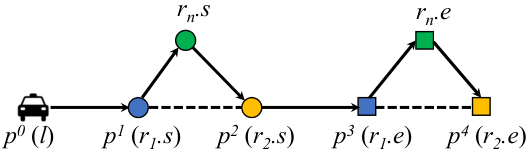
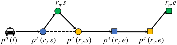
There are three cases shown in Figure 5 when adding a new trip request $r_{n}$ to the trip schedule $c_{i}.S$ of a vehicle $c_{i}$:

1. 1.

   insert-insert: insert $r_{n}.s$ into a segment of $c_{i}.S$ and insert $r_{n}.e$ into the same or another segment of $c_{i}.S$.

2. 2.

   insert-append: insert $r_{n}.s$ into a segment of $c_{i}.S$ and append $r_{n}.e$ to the end of $c_{i}.S$

3. 3.

   append-append: append both $r_{n}.s$ and $r_{n}.e$ to the end of $c_{i}.S$.

We next analyze the conditions that $c_{i}$ needs to satisfy so that adding $r_{n}$ to $c_{i}.S$ is valid for each case.

Insert-insert. Figure 5(a) illustrates the insert-insert case, where both $r_{n}.s$ and $r_{n}.e$ are inserted into some segments of the trip schedule $c_{i}.S$. According to Lemma 2, a segment is valid for inserting a stop only if the stop is inside the detour ellipse of the segment. Therefore, both $r_{n}.s$ and $r_{n}.e$ must be inside the detour ellipse of at least one segment of $c_{i}.S$.

A special case is to insert both $r_{n}.s$ and $r_{n}.e$ to the same segment of $c_{i}.S$, as shown in Figure 6. In this case, both $r_{n}.s$ and $r_{n}.e$ must be inside the detour ellipse of the segment.

The pruning rule for the insert-insert case is as follows:

Insert-append. Figure 5(b) illustrates the insert-append case. According to Lemma 1, to insert $r_{n}.s$, there must be a segment in the trip schedule of $c_{i}$ that has a detour ellipse covering $r_{n}.s$. Meanwhile, any stop between $r_{n}.s$ and $r_{n}.e$ needs to be covered by the detour ellipse of $r_{n}$ (see Lemma 3).

Checking all the stops between $r_{n}.s$ and $r_{n}.e$ against the detour ellipse of $r_{n}$ is non-trivial. For fast pruning, we only check the ending stop of the current trip schedule: if the ending stop is outside of the detour ellipse of $r_{n}$, it is invalid for appending $r_{n}.e$. Take Figure 5(b) as an example. We only check if $p^{4}$ is inside the detour ellipse of $r_{n}$. This simplified rule may bring in a small number of infeasible vehicles, which will be filtered later as explained in the next paragraphs. The pruning rule for the insert-append case is as follows:

Append-append. Figure 5(c) illustrates the append-append case, where we append both $r_{n}.s$ and $r_{n}.e$ to the end of the trip schedule. In this case, $r_{n}$ will not affect any exiting stops. Only the service constraints of $r_{n}$ need to be considered. Furthermore, no stop is scheduled between $r_{n}.s$ and $r_{n}.e$, and hence the detour constraint of $r_{n}$ is satisfied already. The only constraint to check is the waiting time constraint of $r_{n}$. According to Lemma 2, all stops scheduled before $r_{n}.s$ must be covered by the waiting circle of $r_{n}$. For example, in Figure 5(c), the vehicle needs to visit $p^{0},p^{1},p^{2},p^{3},p^{4}$ before picking up $r_{n}.s$. Therefore, all these stops should be covered by the waiting circle of $r_{n}$. Similar to the insert-append case, we only check the ending stop, as summarized in Lemma 7.

In our implementation, we use minimum bounding rectangles (MBRs) to represent ellipses and circles as they are easier to operate on and tightly bound the ellipses and circles.

When a new trip request $r_{n}$ arrives, we first compute the waiting circle and the detour ellipse of $r_{n}$. Then, we compute a set of vehicle candidates that may match $r_{n}$ based on the pruning rules above (Lemmas 5, 6, 7).

To facilitate the pruning, we compute sets of vehicles that:

1. 1.

   have trip schedule segments with detour ellipses that cover $r_{n}.s$ (for the insert-insert and insert-append cases);

2. 2.

   have trip schedule segments with detour ellipses that cover $r_{n}.e$ (for the insert-insert case);

3. 3.

   have the ending stop of the trip schedule covered by $r_{n}.wc$ (for the append-append case);

4. 4.

   have the ending stop of the trip schedule covered by $r_{n}.rd$ (for the insert-append case).

To find vehicles that satisfy a pruning rule, we just need to join the relevant sets of vehicles computed above. For example, vehicles that may satisfy the insert-insert case are those in both the first and the second sets above.

R-tree based pruning. We build two R-trees [17] to accelerate the computation process, although other spatial indices may also be applied. One R-tree stores the detour ellipses of all segments for all vehicle trip schedules, denoted by $T_{seg}$; the other R-tree stores the location of the ending stops of all non-empty vehicles, denoted as $T_{end}$. We run four queries:

1. 1.

   $Q_{1}=T_{seg}.pointQuery(r_{n}.s)$ is a point query that returns all segments whose detour ellipses cover $r_{n}.s$; each segment returned may be used to insert $r_{n}.s$.

2. 2.

   $Q_{2}=T_{seg}.pointQuery(r_{n}.e)$ is a point query that returns all segments whose detour ellipses cover $r_{n}.e$; each segment returned may be used to insert $r_{n}.e$.

3. 3.

   $Q_{3}=T_{end}.rangeQuery(r_{n}.wc)$ is a range query that returns all ending stops covered by $r_{n}.wc$; each ending stop returned may be used to append $r_{n}.s$ and $r_{n}.e$.

4. 4.

   $Q_{4}=T_{end}.rangeQuery(r_{n}.rd)$ is a range query that returns all ending stops covered by $r_{n}.rd$; each ending stop returned may be used to append $r_{n}.e$.

The returned segments and ending stops are further pruned based on their time and capacity constraints. Specifically, for each segment $(p^{k-1},p^{k})$ returned for inserting $r_{n}.s$ ($r_{n}.e$), we check whether the insertion violates the latest arrival time of $p^{k}$ and $r_{n}.s$ ($r_{n}.e$). The schedule between $(p^{k-1},p^{k})$ becomes ($p^{k-1},r_{n}.s(r_{n}.e),p^{k}$) after the insertion. For the new schedule, the arrival time of $r_{n}.s$ ($r_{n}.e$) and $p^{k}$ is estimated based on the arrival time of $p^{k-1}$ plus the travel time between them. If the estimated arrival time of $r_{n}.s(r_{n}.e)$ or $p^{k}$ exceeds their latest arrival time, the segment is discarded. For each ending stop $(p^{m})$ returned for appending $r_{n}.s$ ($r_{n}.e$), we estimate the arrival time of $r_{n}.s$ ($r_{n}.e$) with the appended schedule by summing up the end stop arrival time and the travel time from the end stop to $r_{n}.s$ ($r_{n}.e$). If the estimated time exceeds the latest arrival time of $r_{n}.s$ ($r_{n}.e$), we also discard the ending stop. Besides the time constraint, we also check the capacity constraint for segments to insert $r_{n}.s$. If a segment $(p^{k-1},p^{k})$ is returned for inserting $r_{n}.s$, we sum up the number of passengers carried in $(p^{k-1},p^{k})$ and that of $r_{n}$ and discard the segment if the sum exceeds the capacity.

Let the sets of vehicles corresponding to the segments and ending stops returned by the four queries above (after filtering) be $O_{1}$, $O_{2}$, $O_{3}$ and $O_{4}$, respectively. The set of vehicles satisfying the three pruning cases are: $F_{1}=O_{1}\cap O_{2}$ (insert-insert); $F_{2}=O_{1}\cap O_{4}$ (insert-append); $F_{3}=O_{3}$ (append-append). The union of these three sets, $F=F_{1}\cup F_{2}\cup F_{3}$, is returned as the candidate vehicles.

Processing empty vehicles. Empty vehicles do not have designated trip schedules yet. We only need to check whether they are in the waiting circle of the new request. This can be done by a range query over all empty vehicles using the waiting circle as the query range.

Since our objective is to minimize the system-wide travel time, the optimal empty vehicle is just the nearest one. We thus take a step further and directly compute the optimal empty vehicle with a network nearest neighbor algorithm named IER [15] which has been shown to be highly efficient [13] (other network nearest neighbor algorithms may also apply).

We measure the complexity of our algorithm by the following two parameters $|S|$ and $C$ as they are key to our algorithm: $|S|$ is the maximum number of stops of the vehicle schedules (which is constrained by the vehicle capacity and is a small constant) and $|C|$ is the number of vehicles. We note, however, that instead of using $|S|$, we can use the number of requests $|R|$ instead because there is a linear relationship: $|S||C|\propto|R|$.

Pruning. It takes $O(1)$ time to compute the waiting circle and the detour ellipse of a new request. There are at most $|S||C|$ MBRs in $T_{seg}$ and $|C|$ entries in $T_{end}$. The point query on $T_{seg}$ returns at most $|S||C|$ results and hence the complexity is $O(\sqrt{|S||C|}+|S||C|)$ [18][19]. At most $|C|$ results will be returned from the range query on $T_{end}$ and the complexity is $O(\sqrt{|C|}+|C|)$. The time complexity of the queries on R-trees is thus $O(\sqrt{|S||C|}+|S||C|)$. Checking the time and capacity constraints takes $O(|S||C|+|C|)$ time.

It takes $O(|S||C|+|C|)$ time to retrieve the corresponding vehicles and at most $|C|$ vehicles will be returned in each set after sorting ( $O(|S||C|\log(|S||C|))$ time). The set intersection hence takes O($|C|$) time [20]. The overall time complexity of GeoPrune is thus $O(\sqrt{|S||C|}+|S||C|\log(|S||C|))$.

Update. When a new trip request is assigned to a vehicle $c_{i}$, it takes $O(\log|C|)$ time to delete $c_{i}$ from $T_{ev}$ if $c_{i}$ was empty, $O(|S|\log(|S||C|))$ time to remove invalid segments from $T_{seg}$, and $O(\log|C|)$ time to remove the obsolete record in $T_{end}$ [18][19]. For the new schedule of $c_{i}$, there are at most $|S|$ new segments. It thus takes at $O(|S|)$ time to compute the new detour ellipses for these new segments and $O(|S|\log^{2}(|S||C|))$ time to insert the ellipses to $T_{seg}$ [18][19]. The overall update time for a new request is $O(|S|\log^{2}(|S||C|))$.

References

- [1] http://www.businessofapps.com/data/uber-statistics/.
- [2] S. Ma, Y. Zheng, and O. Wolfson, “T-share: A large-scale dynamic taxi ridesharing service,” in ICDE, 2013, pp. 410–421.
- [3] Y. Tong, Y. Zeng, Z. Zhou, L. Chen, J. Ye, and K. Xu, “A unified approach to route planning for shared mobility,” PVLDB, vol. 11, no. 11, pp. 1633–1646, 2018.
- [4] R. S. Thangaraj, K. Mukherjee, G. Raravi, A. Metrewar, N. Annamaneni, and K. Chattopadhyay, “Xhare-a-Ride: A search optimized dynamic ride sharing system with approximation guarantee,” in ICDE, 2017, pp. 1117–1128.
- [5] Y. Huang, F. Bastani, R. Jin, and X. S. Wang, “Large scale real-time ridesharing with service guarantee on road networks,” PVLDB, vol. 7, no. 14, pp. 2017–2028, 2014.
- [6] J. Alonso-Mora, S. Samaranayake, A. Wallar, E. Frazzoli, and D. Rus, “On-demand high-capacity ride-sharing via dynamic trip-vehicle assignment,” PNAS, vol. 114, no. 3, pp. 462–467, 2017.
- [7] M. Asghari, D. Deng, C. Shahabi, U. Demiryurek, and Y. Li, “Price-aware real-time ride-sharing at scale: an auction-based approach,” in SIGSPATIAL, 2016, p. 3.
- [8] L. Zheng, L. Chen, and J. Ye, “Order dispatch in price-aware ridesharing,” PVLDB, vol. 11, no. 8, pp. 853–865, 2018.
- [9] P. Cheng, H. Xin, and L. Chen, “Utility-aware ridesharing on road networks,” in SIGMOD, 2017, pp. 1197–1210.
- [10] Y. Xu, Y. Tong, Y. Shi, Q. Tao, K. Xu, and W. Li, “An efficient insertion operator in dynamic ridesharing services,” in ICDE, 2019, pp. 1022–1033.
- [11] L. Chen, Q. Zhong, X. Xiao, Y. Gao, P. Jin, and C. S. Jensen, “Price-and-time-aware dynamic ridesharing,” in ICDE, 2018, pp. 1061–1072.
- [12] F. Liu, T. T. Do, and K. A. Hua, “Dynamic range query in spatial network environments,” in DEXA, 2006, pp. 254–265.
- [13] T. Abeywickrama, M. A. Cheema, and D. Taniar, “K-nearest neighbors on road networks: a journey in experimentation and in-memory implementation,” PVLDB, vol. 9, no. 6, pp. 492–503, 2016.
- [14] B. Shen, Y. Zhao, G. Li, W. Zheng, Y. Qin, B. Yuan, and Y. Rao, “V-tree: Efficient knn search on moving objects with road-network constraints,” in ICDE, 2017, pp. 609–620.
- [15] D. Papadias, J. Zhang, N. Mamoulis, and Y. Tao, “Query processing in spatial network databases,” in PVLDB, 2003, pp. 802–813.
- [16] J. J. Pan, G. Li, and J. Hu, “Ridesharing: simulator, benchmark, and evaluation,” Proceedings of the VLDB Endowment, vol. 12, no. 10, pp. 1085–1098, 2019.
- [17] A. Guttman, “R-trees: A dynamic index structurefor spatial searching,” in SIGMOD, 1984, pp. 47–57.
- [18] L. Arge, M. D. Berg, H. Haverkort, and K. Yi, “The priority r-tree: A practically efficient and worst-case optimal r-tree,” ACM Transactions on Algorithms, vol. 4, no. 1, p. 9, 2008.
- [19] Y. Manolopoulos, A. Nanopoulos, A. N. Papadopoulos, and Y. Theodoridis, R-trees: Theory and Applications. Springer Science & Business Media, 2010.
- [20] B. Ding and A. C. König, “Fast set intersection in memory,” PVLDB, vol. 4, no. 4, pp. 255–266, 2011.
- [21] http://nectar.org.au/research-cloud/.
- [22] T. Akiba, Y. Iwata, K.-i. Kawarabayashi, and Y. Kawata, “Fast shortest-path distance queries on road networks by pruned highway labeling,” in ALENEX, 2014, pp. 147–154.
- [23] https://www.openstreetmap.org/.
- [24] https://www1.nyc.gov/site/tlc/about/tlc-trip-record-data.page.
- [25] https://outreach.didichuxing.com/appEn-vue/DataList.
- [26] X. Duan, C. Jin, X. Wang, A. Zhou, and K. Yue, “Real-time personalized taxi-sharing,” in DASFAA, 2016, pp. 451–465.
- [27] L. Zheng, P. Cheng, and L. Chen, “Auction-based order dispatch and pricing in ridesharing,” in ICDE, 2019, pp. 1034–1045.