Deep Learning for Hybrid 5G Services in Mobile Edge Computing Systems: Learn from a Digital TwinThe authors are with the School of Electrical and Information Engineering, University of Sydney, Sydney, NSW 2006, Australia (email: {rui.dong, changyang.she, wibowo.hardjawana, yonghui.li, branka.vucetic}@sydney.edu.au).

In the 5th generation (5G) communication systems, there are diverse applications ranging from high data rate delay tolerant services to ultra-reliable and low-latency communications (URLLC) [1]. By achieving ultra-low end-to-end (E2E) delay and ultra-high reliability, URLLC lies the foundation for emerging latency-critical applications, such as factory automation, autonomous vehicles, and virtual/augmented reality [2]. Devices in these applications will generate some tasks that require to be processed within a short time. To reduce processing time at the local server of each device and to avoid delays in backhauls and core networks, mobile edge computing (MEC) is one promising solution [3]. However, when a task is packetized in a short packet and offloaded to a MEC server via a wireless link, the packet may be lost when the channel is in deep fading [4]. Besides, short blocklength channel codes will cause the none-zero decoding error rate, even for an arbitrarily high signal-to-noise ratio (SNR) [5]. Thus, achieving ultra-high reliability and ultra-low latency is very challenging in MEC systems.

On the other hand, mobile devices have only limited battery capacities. Improving the battery lifetime or energy efficiency (EE) of users is an urgent task [3, 6, 7]. By offloading tasks to MEC servers, we can save energy consumptions at the local servers (equipped at mobile devices), but extra energy is consumed for data transmissions. To minimize the total energy consumption of each user, we need to optimize the offloading probability. In a MEC network with multiple MEC servers and multiple users, the problem that optimizes user association, resource allocation, and offloading probabilities is non-convex and complicated. How to improve EE by solving a non-convex problem in the scenario with both URLLC services and delay tolerant services remains an open problem.

To find the optimal solution to the problem, there are two kinds of approaches: optimization algorithms and machine learning algorithms. Since optimization algorithms need to search the optimal solution when channels change, they are suitable for small-scale problems, such as resource allocation in a single access point (AP) scenario [7, 8]. When the scale of the problem grows, deep learning (DL) algorithms have the potential to find a near optimal solution in a real-time manner [9]. For example, a deep neural network (DNN) can be used as an approximator of an optimal resource allocation policy [9]. The resource allocation obtained from the optimal policy can be used as labeled samples to train the DNN. Once the training of the DNN is finished, we can compute the resource allocation from it with different channel realizations.

To train a DL algorithm, we first need to obtain optimal policies from simplified system models. However, optimal policies may not be available in practical systems. Thus, some other techniques are needed to enable DL algorithms. One approach that does not require labeled training samples is deep reinforcement learning [10]. By learning from the feedback of real-environment, deep reinforcement learning is widely used to maximize long-term rewards of Markov decision processes. This approach is not suitable for URLLC services due to the following two reasons. First, maximizing the long-term reward cannot guarantee the delay and reliability requirements in each time slot. Second, to check whether the packet loss probability satisfies the reliability requirement from the feedback of real network environment, a user needs to transmit a large number of packets. If the required packet loss probability of $10^{-7}$, a user needs to transmit more than $10^{7}$ packets, which may be larger than the total number of packets that will be generated within the service time of the user. To handle this issue, we need to compute the packet loss probability with the help of theoretical results that are obtained with model-based methods.

To merge the model-free deep learning algorithms with model-based theoretical results, we establish a digital twin of the real network environment. As shown in [11], a digital twin is a virtual digital model of the real network that consists of data from the real network (e.g., network topologies, schedulers, and channels) and fundamental rules from theoretical studies (e.g., tradeoffs in information and queueing theories). With the help of a digital twin, we can compute the energy consumption, delay, and packet loss probability of a certain decision on user association and resource allocation. In addition, by monitoring the variations of the real network environment, the system can update the digital twin for training the DNN. As such, it is possible to implement deep learning algorithms in non-stationary environment. Nevertheless, how to apply a digital twin in the DL architecture for hybrid 5G services in MEC systems remains unclear.

Motivated by the above issues, we will answer the following questions in this paper: 1) how to improve EE for URLLC and delay tolerant services in MEC systems? 2) How to establish the digital twin that mirrors the real network environment? 3) How to establish a DL framework based on the digital twin to solve non-convex optimization problems?

In this paper, we would like to improve EE of users in a MEC system, subject to the delay and reliability constraints of URLLC services and the stability constraint of delay tolerant services. A digital twin of the real network is adopted to train the DL algorithm. To the authors’ knowledge, this is the first paper that incorporating the concept of the digital twin with wireless networks. The main contributions of this paper are summarized as follows.

• •

  We propose a digital twin enabled DL framework for improving EE of URLLC and delay tolerant services in a MEC system with multiple APs. The normalized energy consumption, defined as the energy consumption per bit, is minimized by optimizing user association, resource allocation, and offloading probabilities. With this framework, the optimal user association scheme is first explored in the DL framework, and then approximated by a DNN, which is first trained off-line at the central server and then sent the mobility management entity (MME). After the training phase, the central server keeps updating the DNN according to the variation of the real network environment. For a given user association scheme, each AP optimizes the resource allocation and task offloading policy.

• •

  We establish the digital twin of the MEC system, where the network topology, the channel and queueing models, and the fundamental rules are adopted to mirror the real system. In addition, the behavior of each AP, i.e., the optimal resource allocation and task offloading policy, is included in the digital twin. Although the problem at each AP is non-convex, we propose an algorithm that converges to the global optimal solution with linear complexity.

• •

  We design exploration policies that generate multiple user association schemes in each learning epoch. For each user association scheme, the normalized energy consumption, delay, and reliability are evaluated in the digital twin. Then, the best one is saved in the memory as labeled training samples. To compare the efficiency of different exploration policies, the normalized energy efficiency and computing complexity of different exploration policies are illustrated with simulation results.

Furthermore, simulation results show that the proposed DL framework can achieve a lower normalized energy consumption with less computing complexity compared with an existing solution, and can approach to the global optimal solution.

We consider a MEC system shown in Fig. 1, where $M$ APs serve $K^{\rm u}$ URLLC services and $K^{\rm b}$ delay tolerant services, which are indexed by $\mathcal{K}^{\rm u}=\{1,...,K^{\rm u}\}$ and $\mathcal{K}^{\rm b}=\{K^{\rm u}+1,...,K^{\rm u}+K^{\rm b}\}$, respectively. For notational simplicity, we use a superscript $\xi=\{\rm u,\rm b\}$ to represent the types of services in this work. If $\xi={\rm u}$, a parameter is used in URLLC services. Otherwise, it is used in delay tolerant services. All the notations used in this paper are listed in Table I.

The APs are connected to the MME that is in charge of user association. To establish the digital twin, the MME sends some parameters and models of the network to a central server, where the user association scheme is optimized by a DL algorithm that learns from the digital twin. After the training phase, a DNN for user association is sent to the MME. With a given user association scheme, the network can be decomposed into single-AP problems.¹¹ 1 Frequency reuse factor is less than one that different bandwidth is allocated to adjacent APs. As such, there is no strong interference, and weak interferences are considered as noise. For each single-AP problem, the AP optimizes resource allocation and task offloading for users that are associated with it.

Each AP is equipped with a MEC server and each user has a local server. Time is discretized into slots. The duration of each slot is $T_{\rm s}$. The service rates of the $m$th MEC server and the $k$th user are denoted as $S_{m}$ (CPU cycles/slot) and $C_{k}^{\xi}$ (CPU cycles/slot), respectively. The $k$th user can adjust $C_{k}^{\xi}$ within the regime $[0,C_{k}^{\max,\xi}]$, where $C_{k}^{\max,\xi}$ is the maximum computing capacity of the user.

Without loss of the generality, non-stationary parameters in a system can be classified into two categories. The first category of parameters is highly dynamic, such as the large-scale channel gains and the average task arrival rates. The other category of parameters varies slowly, such as the density of users in a certain area. For the first category of parameters, we include them in the input of the DNN. For the second category of parameters, the system monitors their values and updates them in the digital twin. Then, the DNN learns from the updated digital twin. Rather than training a new DNN, the previous well-trained DNN will be used to initialize the new DNN. In this way, the output of the DNN changes with non-stationary parameters.

The computation tasks of the $k$th user are characterized by $(\lambda_{k}^{\xi},b_{k}^{\xi},c_{k}^{\xi})$, where $\lambda_{k}^{\xi}$ (packets/slot) is the average task arrival rate generated by the $k$th user, $b_{k}^{\xi}$ (bits/packet) is the number of bits of each task (i.e., the size of a packet), and $c_{k}^{\xi}$ (cycles/packet) is the number of CPU cycles required to process each task. We assume that each task is conveyed in one packet, and the relation between $b_{k}^{\xi}$ and $c_{k}^{\xi}$ is given by $c_{k}^{\xi}=k_{1}b_{k}^{\xi}$, where $k_{1}>0$ (cycles/bit) depends on the computational complexity of the task [21, 22, 23].

For URLLC services, we assume that the packet size and the number of CPU cycles required to process each packet are constant (e.g., $32$ bytes [1]), and the packet arrival process follows a Bernoulli process. In each slot, a user either has a packet to transmit or stays silent. For delay tolerant services, both the inter-arrival time between packets and the packet size may follow any general distributions. The only assumption is that the packet size of delay tolerant services is much longer than that of URLLC services. In the rest of the paper, the tasks of URLLC services and delay tolerant services are referred to as short and long packets, respectively.

The users can offload tasks to one of the MEC servers via wireless links. Let $\boldsymbol{\beta}$ be the user association vector with entry $\beta_{m,k}^{\xi}$ denoting whether the $k$th user is associated with the $m$th AP. If the $k$th user is associated with the $m$th AP, then $\beta_{m,k}^{\xi}=1$. Otherwise, $\beta_{m,k}^{\xi}=0$. We assume that each user can only offload packets to one of the APs, i.e., $\sum_{m\in\mathcal{M}}\beta_{m,k}^{\xi}=1$, where $\mathcal{M}={1,...,M}$ is the set of indices of APs.

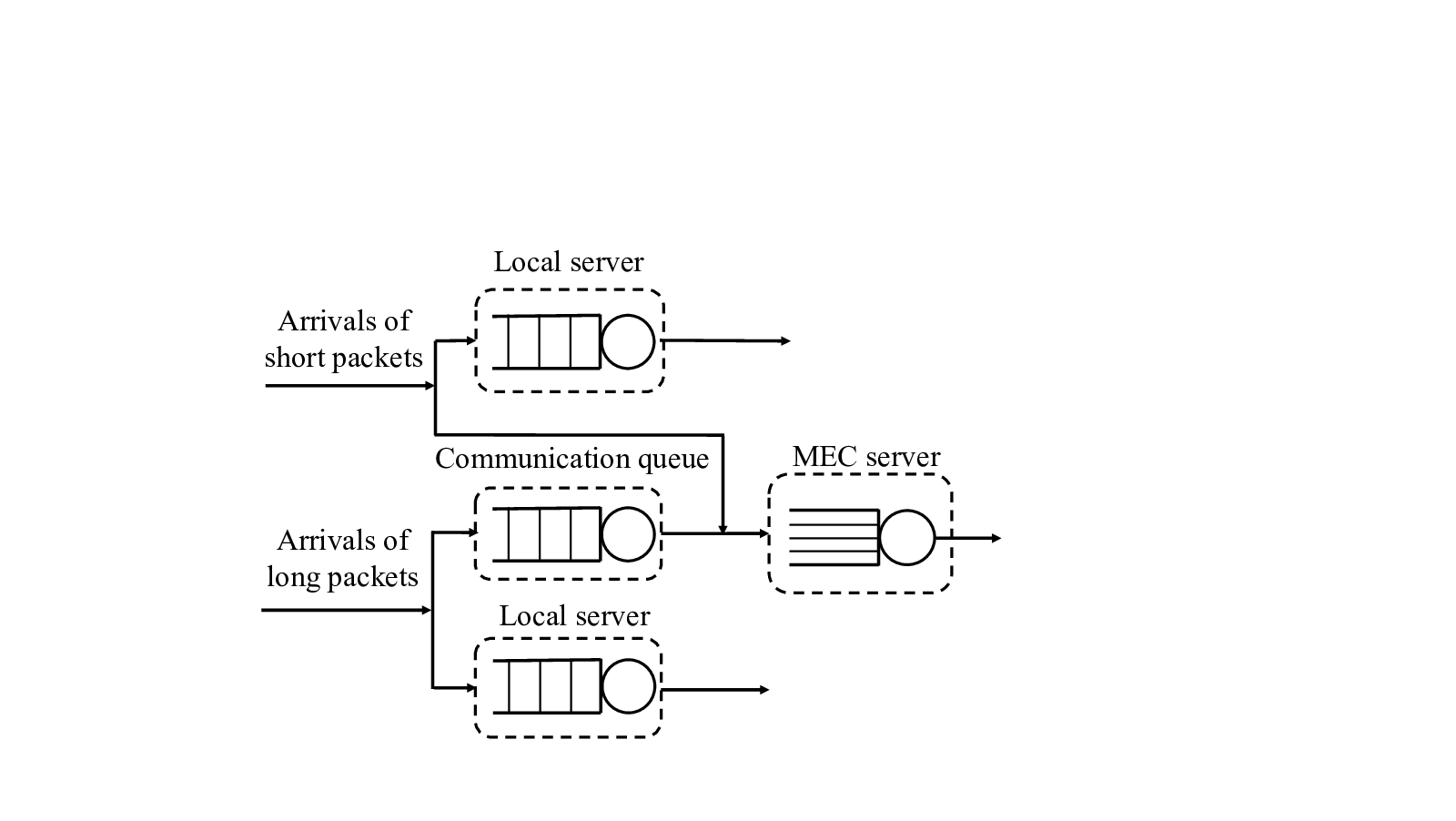
The queueing models of the local servers and the MEC servers are illustrated in Fig. 2. In the local servers, packets are served according to the first-come-first-serve (FCFS) order. The difference between URLLC and delay tolerant services lies in the queueing model before uplink transmission. For URLLC services, each packet is transmitted in one slot. Since the packet arrival process follows a Bernoulli process, the peak arrival rate is one packet per slot, which is equal to the transmission rate of the wireless link. As a result, there is no queue before uplink transmission. For delay tolerant services, the peak arrival rate can be higher than the transmission rate, and hence some packets may wait in a communication queue before uplink transmission.

In the MEC servers, there are short and long packets. If the packets are served according to FCFS order, short packets arrive at the MEC servers after a long packet need to wait for the processing of the long packet. To avoid long queueing delay, a processor-sharing (PS) server is adopted at each AP [24]. On the PS server, the service rate of the server is equally allocated to all the packets in the server. When there are $i$ packets in the $m$th server, the service rate of each packet is $S_{m}/i$. As shown in [25], when there are short and long packets, the PS server outperforms the FCFS server.

Let $e_{k}^{\rm loc,\xi}$ be the energy consumption per CPU cycle of the $k$th user. According to the measurements in [26, 21], $e_{k}^{\rm loc,\xi}=k_{0}(C_{k}^{\xi})^{2}$ (J/cycle), where $k_{0}$ is a coefficient depending on the chip architecture. The typical value of $k_{0}$ is $10^{-15}$. The energy consumption per packet at the local server is

which indicates that the energy consumption for processing one packet increases with the processing rate $C_{k}^{\xi}$.

The E2E delay of a packet is defined as the interval between the arrival time of a packet and the time when the processing of the packet is finished. For URLLC service, we denote $D^{\max,\rm u}$ and $\epsilon^{\max,\rm u}$ as the required delay bound and the maximal threshold of the tolerable delay bound violation probability, respectively.

For delay tolerant services, we only need to ensure the queueing system is stable, i.e., the average service rate is equal to or higher than the average arrival rate.

Our goal is to minimize the normalized energy consumption, defined as the energy consumption per bit.

To avoid the users with bad channel conditions or high task arrival rates experiencing high energy consumption, we take fairness among all the users into consideration by minimizing the maximal normalized energy consumption of the $K^{\rm u}+K^{\rm b}$ users. If there is a central control plane that manages user association and resource allocation, the optimization problem can be formulated as follows,

where $N^{\max}$ is the total number of subcarriers of each AP and $P_{k}^{\max,\xi}$ is the maximal transmit power of the $k$th user. Constraint (19d) is obtained from (13) and (16). Since the required transmit power is determined by the bandwidth allocation and the offloading probability, it can be removed from the optimization variables. The relation between the optimal solution and the inputs, i.e., large-scale channel gains and average task arrival rates, is denoted as $\pi_{1}:=\boldsymbol{\alpha},{\boldsymbol{\lambda}}\rightarrow\boldsymbol{\beta}^{*},\boldsymbol{N}^{*},\boldsymbol{x}^{*}$, where $\boldsymbol{\alpha}=({\boldsymbol{\alpha}}^{\rm u}_{1},...,{\boldsymbol{\alpha}}^{\rm u}_{K^{\rm u}},{\boldsymbol{\alpha}}^{\rm b}_{1},...,{\boldsymbol{\alpha}}^{\rm b}_{K^{\rm b}})^{\rm T}$, ${\boldsymbol{\alpha}}^{\xi}_{k}=(\alpha^{\xi}_{1,k},...,\alpha^{\xi}_{M,k})^{\rm T}$, $\boldsymbol{\lambda}=({{\lambda}}^{\rm u}_{1},...,{{\lambda}}^{\rm u}_{K^{\rm u}},{{\lambda}}^{\rm b}_{1},...,{{\lambda}}^{\rm b}_{K^{\rm b}})^{\rm T}$, $\boldsymbol{\beta}=({\boldsymbol{\beta}}^{\rm u}_{1},...,{\boldsymbol{\beta}}^{\rm u}_{K^{\rm u}},{\boldsymbol{\beta}}^{\rm b}_{1},...,{\boldsymbol{\beta}}^{\rm b}_{K^{\rm b}})^{\rm T}$, ${\boldsymbol{\beta}}^{\xi}_{k}=(\beta^{\xi}_{1,k},...,\beta^{\xi}_{M,k})^{\rm T}$, $\boldsymbol{N}=({\boldsymbol{N}}^{\rm u}_{1},...,{\boldsymbol{N}}^{\rm u}_{K^{\rm u}},{\boldsymbol{N}}^{\rm b}_{1},...,{\boldsymbol{N}}^{\rm b}_{K^{\rm b}})^{\rm T}$, ${\boldsymbol{N}}^{\xi}_{k}=(N^{\xi}_{1,k},...,N^{\xi}_{M,k})^{\rm T}$, $\boldsymbol{x}=({{x}}^{\rm u}_{1},...,{{x}}^{\rm u}_{K^{\rm u}},{{x}}^{\rm b}_{1},...,{{x}}^{\rm b}_{K^{\rm b}})^{\rm T}$, and $(\cdot)^{\rm T}$ denotes the transpose operator.

In practice, a user can subscribe to both kinds of services. If the $k$th user subscribes to both kinds of services, $\lambda_{k}^{\rm u}$ and $\lambda_{k}^{\rm b}$ are referred to as the average task arrival rates of URLLC and delay tolerant services, respectively. The large-scale channel gains of the two kinds of services are the same, i.e., $\alpha_{k}^{\rm u}=\alpha_{k}^{\rm b}$. In the local server of the $k$th user, the packets from different services are waiting in two separated FCFS queues. The energy consumption per packet in (4) becomes $E_{k}^{\rm loc}=k_{0}(C_{k})^{2}(c_{k}^{\rm u}+c_{k}^{\rm b})$. The transmit power constraint of the $k$th user becomes $P_{k}^{\rm u}+P_{k}^{\rm d}\leq P_{k}^{\max}$. The rest of the constraints remains the same.

Note that user association is managed by MME, but resource allocation and offloading probabilities are determined by each AP. The problem $\mathcal{P}_{1}$ is decomposed into two subproblems that are solved in two timescales at MME and APs, respectively. In the first subproblem, each AP optimizes resource allocation and offloading probabilities with given user association scheme. In the second subproblem, the MME optimizes user association scheme with a DL algorithm, where the behavior of each AP (i.e., the optimal resource allocation and task offloading policy) is taken into account.

• •

  Problem $\mathcal{P}_{2}$: The problem that optimizes subcarrier allocation and offloading probability can be formulated as follows,

  	$\displaystyle\mathcal{P}_{2}:$	$\displaystyle\min_{N_{m,k}^{\xi},x_{k}^{\xi}}\max_{k\in\mathcal{K}^{\xi}}\eta_{k}^{\xi},$		(20)
  		$\displaystyle\text{s.t.}\;\eqref{stx},\eqref{stN},\eqref{strho},\eqref{stC},\eqref{stP},\eqref{R_k^U},\eqref{rb},\eqref{dloc},\eqref{eloc},\eqref{t-mec},\eqref{t-mec3},\eqref{embblocser}\text{ and }\eqref{embbre}.$

  The relation between the optimal $(\boldsymbol{N}^{*},\boldsymbol{x}^{*})$ and $(\boldsymbol{\alpha},\boldsymbol{\lambda},\boldsymbol{\beta})$ is denoted as $\pi_{2}:=\boldsymbol{\alpha},\boldsymbol{\lambda},\boldsymbol{\beta}\rightarrow\,\boldsymbol{N}^{*},\boldsymbol{x}^{*}$. The minimal normalized energy consumption achieved with $\pi_{2}$ is denoted as $Q^{*}_{2}(\boldsymbol{\alpha},\boldsymbol{\lambda},\boldsymbol{\beta}|\pi_{2})$, which indicates that the normalized energy consumption depends on the user association.

• •

  Problem $\mathcal{P}3$: The problem that optimizes user association scheme can be formulated as follows,

  	$\displaystyle\mathcal{P}_{3}:$	$\displaystyle\min_{\beta_{m,k}^{\xi}}Q^{*}_{2}(\boldsymbol{\alpha},\boldsymbol{\lambda},\boldsymbol{\beta}|\pi_{2}),$		(21)
  		s.t. (19c)

  The relation between the optimal $\boldsymbol{\beta}^{*}$ and $\boldsymbol{\alpha},\boldsymbol{\lambda}$ is denoted as $\pi_{3}:=\boldsymbol{\alpha},\boldsymbol{\lambda}\mathop{\to}\boldsymbol{\beta}^{*}$. The minimal normalized energy consumption achieved with $\pi_{3}$ is denoted as $Q^{*}_{3}(\boldsymbol{\alpha},\boldsymbol{\lambda}|\pi_{2},\pi_{3})$, which also depends on $\pi_{2}$.

It is worth noting that both $\mathcal{P}_{2}$ and $\mathcal{P}_{3}$ are non-convex. We will propose an optimization algorithm to solve problem $\mathcal{P}_{2}$ and apply the deep learning algorithm to solve problem $\mathcal{P}_{3}$.

The framework of the digital twin enabled DL algorithm is illustrated in Fig. 3. The inputs of the DNN are the large-scale channel gains from users to APs and the average task arrival rates of all the users, while the output of the DNN is the user association scheme. The direct output of the DNN is denoted as $\hat{\boldsymbol{{\beta}}}$, based on which we explore user association schemes. For a user association scheme, we can obtain the related normalized energy consumption from the digital twin. From the feedback of the digital twin, we find the best user association scheme, $\tilde{\boldsymbol{{\beta}}}$, that minimizes the normalized energy consumption among the user association schemes randomly generated according to exploration policies. Finally, the inputs $\boldsymbol{{\alpha}},\boldsymbol{\lambda}$ and the best output $\tilde{\boldsymbol{{\beta}}}$ are saved in the memory and will be used to train the DNN.

From problem $\mathcal{P}_{2}$ we can see that only constraints (19b) and (19d) depend on the optimization variables of all the users, and the other constraints only depend on the resource allocation and offloading probability of a single user. To solve problem $\mathcal{P}_{2}$, we first remove constraints (19b) and (19d) and decompose the problem into multiple single-user problems. After solving these single-user problems, we check whether constraints (19b) and (19d) are satisfied or not. The algorithm is summarized in Table II.

To remove constraint (19b), we first find the minimum of the maximal normalized energy consumption via binary search. For a given value of $\eta^{\rm th}$, we minimize the total number of subcarriers that is required to guarantee $\max_{k\in\mathcal{K}^{\xi}}\eta_{k}^{\xi}\leq\eta^{\rm th}$, i.e.,

If the required bandwidth is larger than $N^{\max}$, $\eta^{\rm th}$ cannot be achieved, and the minimum of $\max_{k\in\mathcal{K}^{\xi}}\eta_{k}^{\xi}$ is higher than $\eta^{\rm th}$. Otherwise, the minimum of $\max_{k\in\mathcal{K}^{\xi}}\eta_{k}^{\xi}$ is lower than $\eta^{\rm th}$. Via binary search, $\eta^{\rm th}$ converges to the minimum of $\max_{k\in\mathcal{K}^{\xi}}\eta_{k}^{\xi}$, and the corresponding bandwidth allocation and offloading probabilities are the optimal solution of problem $\mathcal{P}_{2}$ (See proof in Subsection V-C.).

In the second step, we remove constraint (19d), and decompose problem (22) into multiple single-user problems. For each single-user problem, we search the minimum number of subcarriers allocated to each user via binary search. For a given value of $N_{k}^{\rm th,\xi}$, we minimize $\eta^{\xi}_{k}$ subject to $N_{k}^{\xi}=N_{k}^{\rm th,\xi}$, i.e.,

If $\eta^{\xi}_{k}\leq\eta^{\rm th}$, then $N_{k}^{\xi*}\leq N_{k}^{\rm th,\xi}$. Otherwise, $N_{k}^{\xi*}\geq N_{k}^{\rm th,\xi}$ (See proof in Subsection V-C). Thus, $N_{k}^{\rm th,\xi}$ either converges the minimum of $N_{k}^{\xi}$ or $N^{\max}$ (i.e., $\eta^{\xi}_{k}>\eta^{\rm th}$ even with $N_{k}^{\xi}=N^{\max}$ ).

After obtaining the solutions of the single-user problems, we to check whether constraints (19b) and (19d) are satisfied or not in Line 23 of the algorithm in Table II.

If constraints (19b) and (19d) cannot be satisfied by the end of the binary search, problem $\mathcal{P}_{2}$ is infeasible and the AP cannot guarantee the QoS requirements of all the users associated with it. In this case, the normalized energy consumption of the user association scheme will be set as infinite in the learning framework in Fig. 3. This user association scheme will not be used to train the DNN since the QoS requirements cannot be satisfied.

In this subsection, we show how to solve problem (23). Since the offloading probability depends on bandwidth allocation, we denote the optimal offloading probability as $\hat{x}_{k}^{\xi}(N_{k}^{\rm{th,\xi}})$.

In this subsection, we first prove that for a given threshold of the normalized energy consumption, $\eta^{\rm th}$, the algorithm in Table II can find the minimum bandwidth that is required to achieve the threshold (From Line 4 to Line 22 in Table II). To prove it, we only need to prove that the normalized energy consumption decreases with $N_{k}^{\rm th,\xi}$.

The above property indicates that the binary search converges to the minimal $N_{k}^{\rm th,\xi}$ that can guarantee $\eta_{k}\leq\eta^{\rm th}$, unless it is infeasible (as shown in Line 20 of Table II).

To find out whether problem $\mathcal{P}_{2}$ is feasible or not, we minimize the total number of subcarriers and see whether it is less than the total number of subcarriers of an AP. Besides, we also need to minimize the total offloading probability and see whether it satisfies the constraint in (19d).²² 2 The rest of the constraints are satisfied with the solution of problem (23). The following property indicates that minimizing the offloading probability of the $k$th user is equivalent to minimizing the number of subcarriers allocated to it.

Therefore, by minimizing the sum of the numbers of subcarriers, we also obtained the minimum of the sum of the offloading probabilities. In other words, both the sum of the numbers of subcarriers and the workload at the MEC server are minimized with the algorithm from Line 4 to Line 22 in Table II. As a result, problem $\mathcal{P}_{2}$ is feasible if and only if constraints (19b) and (19d) are satisfied with $N_{k}^{\rm{th},\xi}$ and $\hat{x}_{k}^{\xi}(N_{k}^{\rm{th},\xi})$, i.e., the condition in Line 23 in Table II.

If problem $\mathcal{P}_{2}$ is feasible when the normalized energy consumption equals $\eta^{\rm th}$, then $\eta^{\rm th}$ is achievable and the minimal normalized energy consumption $\eta^{*}\leq\eta^{\rm th}$. Otherwise, $\eta^{*}>\eta^{\rm th}$. Therefore, with the binary search (i.e., Lines 2,3 and Lines 23 to 27), $\eta^{\rm th}$ converges to $\eta^{*}$. The coresponding $N_{k}^{\rm{th},\xi}$ and $\hat{x}_{k}^{\xi}(N_{k}^{\rm{th},\xi})$ converge to the optimal solution $N_{k}^{\xi*}$ and $x_{k}^{\xi*}$.

Given the required searching precision of the normalized energy consumption $\sigma_{\eta}$, it takes $\mathcal{O}\left(\log_{2}(\frac{\eta^{\rm ub}}{\sigma_{\eta}})\right)$ steps to obtain the minimum of the maximal normalized energy consumption of all the users. To achieve a target $\eta^{\rm th}$, $(K^{\rm u}+K^{\rm b})\mathcal{O}\left(\log_{2}(\frac{N_{k}^{{\rm ub},\xi}}{\sigma_{N}})\right)$ steps are needed to obtain the required numbers of subcarriers of $K^{\rm u}+K^{\rm b}$ users, where $\sigma_{N}$ is the required searching precision of the number of subcarriers. For a given number of subcarriers, it takes $\mathcal{O}\left(\log_{2}(\frac{1}{\sigma_{x}})\right)$ steps to obtain the optimal offloading probability that minimizes the normalized energy consumption of the delay tolerant user in the region $[0,1]$, where $\sigma_{x}$ is the required searching precision of offloading probability. For URLLC services, the optimal offloading probability can be obtained in the closed-form expression in (29). Therefore, the complexity of the algorithm can be expressed as $(K^{\rm u}+K^{\rm b})\mathcal{O}\left(\log_{2}(\frac{\eta^{\rm ub}}{\sigma_{\eta}})\log_{2}(\frac{N_{k}^{{\rm ub},\xi}}{\sigma_{N}})\log_{2}(\frac{1}{\sigma_{x}})\right)$, which increases linearly with $(K^{\rm u}+K^{\rm b})$.

References

- [1] 3GPP TSG RAN TR38.913 R14, “Study on scenarios and requirements for next generation access technologies,” Jun. 2017.
- [2] P. Schulz, M. Matthé, H. Klessig, et al., “Latency critical IoT applications in 5G: Perspective on the design of radio interface and network architecture,” IEEE Commun. Mag., vol. 55, no. 2, pp. 70–78, Feb. 2017.
- [3] Y. Mao, C. You, J. Zhang, K. Huang, and K. B. Letaief, “A survey on mobile edge computing: The communication perspective,” IEEE Commun. Surveys Tuts., vol. 19, no. 4, pp. 2322–2358, 2017.
- [4] C. She, C. Yang, and T. Q. S. Quek, “Cross-layer optimization for ultra-reliable and low-latency radio access networks,” IEEE Trans. Wireless Commun., vol. 17, no. 1, pp. 127–141, Jan. 2018.
- [5] W. Yang, G. Durisi, T. Koch, and Y. Polyanskiy, “Quasi-static multiple-antenna fading channels at finite blocklength,” IEEE Trans. Inf. Theory, vol. 60, no. 7, pp. 4232–4264, Jul. 2014.
- [6] K. Cheng, Y. Teng, W. Sun, A. Liu, and X. Wang, “Energy-efficient joint offloading and wireless resource allocation strategy in multi-MEC server systems,” 2018. [Online]. Available: https://arxiv.org/pdf/1803.07243v1.pdf
- [7] J. Zhang, X. Hu, Z. Ning, E. C. . Ngai, L. Zhou, J. Wei, J. Cheng, and B. Hu, “Energy-latency tradeoff for energy-aware offloading in mobile edge computing networks,” IEEE Internet Things J., vol. 5, no. 4, pp. 2633–2645, Aug. 2018.
- [8] C. You, Y. Zeng, R. Zhang, and K. Huang, “Asynchronous mobile-edge computation offloading: energy-efficient resource management,” 2018. [Online]. Available: https://arxiv.org/abs/1801.03668
- [9] J. Guo, C. Yang, and C.-L. I, “Exploiting future radio resources with end-to-end prediction by deep learning,” IEEE Access, vol. 6, pp. 75 729–75 747, Nov. 2018.
- [10] N. C. Luong, D. T. Hoang, S. Gong et al., “Applications of deep reinforcement learning in communications and networking: A survey,” submitted to IEEE Commun. Surveys Tuts., 2018. [Online]. Available: https://arxiv.org/pdf/1810.07862.pdf
- [11] M. Wise, “APM: Driving value with the digital twin,” in GE Digital, 2017.
- [12] K. Cheng, Y. Teng, W. Sun, A. Liu, and X. Wang, “Energy-efficient joint offloading and wireless resource allocation strategy in multi-MEC server systems,” in Proc. IEEE ICC, 2018.
- [13] S.-W. Ko, K. Han, and K. Huang, “Wireless networks for mobile edge computing: Spatial modelling and latency analysis,” IEEE Trans. on Wireless Commun., vol. 17, no. 8, pp. 5225–5240, Aug. 2018.
- [14] J. Zhou, X. Zhang, and W. Wang, “Joint resource allocation and user association for heterogeneous services in multi-access edge computing networks,” IEEE Access, vol. 7, pp. 12 272–12 282, Jan. 2019.
- [15] X. Chen, H. Zhang, C. Wu, S. Mao, Y. Ji, and M. Bennis, “Performance optimization in mobile-edge computing via deep reinforcement learning,” 2018. [Online]. Available: https://arxiv.org/abs/1804.00514v1
- [16] M. Min, D. Xu, L. Xiao, Y. Tang, and D. Wu, “Learning-based computation offloading for iot devices with energy harvesting,” 2017. [Online]. Available: https://arxiv.org/abs/1712.08768v1
- [17] J. Xu, L. Chen, and S. Ren, “Online learning for offloading and autoscaling in energy harvesting mobile edge computing,” IEEE Trans. Cogn. Commun. Netw., vol. 3, no. 3, pp. 361–373, Sept. 2017.
- [18] L. Huang, S. Bi, and Y.-J. A. Zhang, “Deep reinforcement learning for online offloading in wireless powered mobile-edge computing networks,” Sept. 2018. [Online]. Available: http://arxiv.org/abs/1808.01977
- [19] C.-F. Liu, M. Bennis, and H. V. Poor, “Latency and reliability-aware task offloading and resource allocation for mobile edge computing,” in Proc. IEEE Globecom, 2017.
- [20] J. Liu and Q. Zhang, “Offloading schemes in mobile edge computing for ultra-reliable low latency communications,” IEEE Access, vol. 6, pp. 12 825–12 837, 2018.
- [21] A. P. Miettinen and J. K. Nurminen, “Energy efficiency of mobile clients in cloud computing.” HotCloud, vol. 10, pp. 4–4, 2010.
- [22] O. Munoz, A. Pascual-Iserte, and J. Vidal, “Optimization of radio and computational resources for energy efficiency in latency-constrained application offloading,” IEEE Trans. Veh. Technol., vol. 64, no. 10, pp. 4738–4755, Oct. 2015.
- [23] Y. Wang, M. Sheng, X. Wang, L. Wang, and J. Li, “Mobile-edge computing: Partial computation offloading using dynamic voltage scaling,” IEEE Trans. Commun., vol. 64, no. 10, pp. 4268–4282, Oct. 2016.
- [24] M. Harchol-Balter, Performance Modeling and Design of Computer Systems: Queueing Theory in Action. Cambridge University Press, 2013.
- [25] Y. Duan, C. She, G. Zhao, and T. Q. S. Quek, “Delay analysis and computing offloading of URLLC in mobile edge computing systems,” in Proc. WCSP, 2018.
- [26] W. Zhang, Y. Wen, K. Guan, D. Kilper, H. Luo, and D. O. Wu, “Energy-optimal mobile cloud computing under stochastic wireless channel,” IEEE Trans. Wireless Commun., vol. 12, no. 9, pp. 4569–4581, Sept. 2013.
- [27] A. Gravey, J.-R. Louvion, and P. Boyer, “On the Geo/D/1 and Geo/D/1/N queues,” Perform. Eval., vol. 11, no. 2, pp. 117–125, Jul. 1990. [Online]. Available: http://dx.doi.org/10.1016/0166-5316(90)90018-E
- [28] S. Schiessl, J. Gross, and H. Al-Zubaidy, “Delay analysis for wireless fading channels with finite blocklength channel coding,” in Proc. ACM MSWiM, 2015.
- [29] C. Sun, C. She, C. Yang, T. Q. Quek, Y. Li, and B. Vucetic, “Optimizing resource allocation in the short blocklength regime for ultra-reliable and low-latency communications,” IEEE Trans. Wireless Commun., 2018.
- [30] V. Mnih, K. Kavukcuoglu, D. Silver et al., “Human-level control through deep reinforcement learning,” Nature, vol. 518, no. 7540, pp. 529–533, Feb. 2015.
- [31] D. P. Kingma and J. Ba, “Adam: A method for stochastic optimization,” 2014. [Online]. Available: http://dblp.uni-trier.de/db/journals/corr/corr1412.htmlKingmaB14
- [32] 3GPP, LTE ETSI TR 36.931 v9.0.0, “Evolved universal terrestrial radio access.” May 2011.
- [33] Z. Hou, C. She, Y. Li, T. Q. S. Quek, and B. Vucetic, “Burstiness aware bandwidth reservation for ultra-reliable and low-latency communications (URLLC) in tactile internet,” IEEE J. Sel. Areas Commun., vol. 36, no. 11, pp. 1–10, Nov. 2018.
- [34] S. Boyd and L. Vandenberghe, Convex Optimization. New York, NY, USA: Cambridge University Press, 2004.