Multi-Frequency Atom-Photon InteractionsPreprint: APS/123-QED

We consider a two-level system, such as an atom, interacting with a multi-frequency field with fundamental frequency $\omega_{f}$ ¹¹ 1 The frequency $\omega_{f}$ need only be the greatest common denominator of the frequencies under consideration, but in principle could be the fundamental frequency $2\pi c/L$ when one imposes periodic boundary conditions to quantise the electromagnetic field. Thus, requiring that the field frequencies are rationally related in this model is not an overly restrictive assumption., described by the polychromatic Jaynes-Cummings model with Hamiltonian

The rotating-wave approximation has been made and this form is relevant for the systems considered in Sec. III and Sec. IV; the Rabi model without this approximation is treated in Sec. V. In this model $\pm\tfrac{1}{2}\omega_{0}$ are the spin eigenenergies, the field modes are indexed by $i$ and the $i^{\mathrm{th}}$ mode has frequency $k_{i}\omega_{f}$ where $k_{i}$ are integers and need not be commensurate. $g_{k_{i}}$ are the coupling spin-field constants. More generally the mode frequencies do not need to be commensurate.

A natural basis to describe the coupled atoms and photons comprises of Fock-spin states $\ket{n_{k_1},n_{k_2},... ,m}$, where $n_{k_{i}}$ is the number of photons in mode $k_{i}$ and $m\hbar$ the atom’s spin projection. These are eigenstates of $H_{0}=\tfrac{1}{2}\omega_{0}\sigma_{z}+\sum_{\{k\}}k\omega_{f}a_{k}^{\dagger}a_{k}$ and an extension of the basis $\{\ket{n,m}|n\in\mathds{Z}^{+},m=\pm\tfrac{1}{2}\}$ used extensively for the single-frequency Jaynes-Cummings model. However, calculations performed in this basis are often divergent. The problems associated with this basis for the multi-frequency model are caused by (i) the nature of multi-frequency interaction $V=\sum_{\{k\}}g_{k}\left(a_{k}\sigma_{+}+a_{k}^{\dagger}\sigma_{-}\right)$ and (ii) degeneracy of these states. In section II we introduce a new non-degenerate basis upon which the dynamics of the multi-frequency model Eq. 1 can be solved using a wide range of conventional methods. In the remainder of this section we elaborate on the key differences between the single and multi-frequency Jaynes-Cummings model and the problem of working with Fock-spin states.

In striking contrast to the single-frequency model is that a vast number of different states can now interact with each other. For a single-frequency field only pairs of states $\ket{n,-\tfrac 12}$ and $\ket{n-1,\tfrac 12}$ are permitted to interact - under the rotating wave approximation - by the terms $a\sigma_{+}$ and $a^{\dagger}\sigma_{-}$. For multiple frequencies, atoms can climb the Jaynes-Cummings ladder by interacting on alternate modes. The extended range of interactions, together with energy degeneracies of the Fock states $\ket{n_1,n_2,...}$ cause the standard numerical or perturbative approaches to breakdown due to divergences in their solutions.

It is well known for example, that an energy degeneracy between a pair of interacting states $\ket{\psi_1}$ and $\ket{\psi_2}$ causes the perturbative solutions to the Schrödinger equation to diverge due to the energy denominator $E_{1}-E_{2}=0$. Such degeneracies are common for multi-frequency fields of Eq. 1. Consider for example a field with three commensurate frequencies (i.e. $k_{1}$, $k_{2}=k_{1}+1$ and $k_{3}=k_{1}+2$), and the interaction between states $\ket{n_1,n_2,n_3,m}$ and $\ket{n_1+1,n_2-2,n_3+1,m}$. These states are degenerate since $k_{1}-2k_{2}+k_{3}=0$. They also interact via a fourth order interaction $\propto a_{k_{1}}^{\dagger}\sigma_{-}a_{k_{2}}\sigma_{+}a_{k_{3}}^{\dagger}\sigma_{-}a_{k_{2}}\sigma_{+}$. The energy shift caused by this interaction incorrectly appears to diverge when calculated perturbatively. So called ‘non perturbative’ analytic methods such as the resolvent formalism employed in Sec. IV also suffer from such degeneracies for the same reason.

Simple numerical approaches also suffer from these degeneracies. To diagonalise Eq. 1 numerically we must truncate the basis over a finite range of values $n_{k}$ for each mode. An efficient truncation method starts with state $\ket{n_1,n_2,n_3,-\tfrac 12}$ for a three mode field for example, and includes any states which can be connected by applying $a_{k}\sigma_{+}$ and $a_{k}^{\dagger}\sigma_{-}$ up to some maximum number $N$ times. For example, including up to $N=1$ interactions, the basis consists of $\ket{n_1,n_2,n_3,-\tfrac 12}$ together with $\ket{n_1-1, n_2, n_3,\tfrac 12},\ \ket{n_1, n_2-1 , n_3,\tfrac 12}$ and $\ket{n_1, n_2, n_3-1,\tfrac 12}$. For $N=2$ our basis includes six further states connected to $\ket{n_{k_1}, n_{k_2}, n_{k_3},-\tfrac 12}$ via $a_{k_{j}}^{\dagger}\sigma_{-}a_{k_{i}}\sigma_{+}$ for all combinations $i\neq j$. The truncated basis is shown diagrammatically in Fig. 1a for $N=3$ along with their energies. Even in this limited basis degeneracies are abundant; There are seven pairs of states which have the same energy and spin.

The problem encountered numerically is that the basis must be truncated and subsequently the degenerate states are not all surrounded by a similar set of interactions. Look for example at the state spin up state $\ket{n_1,n_2-1,n_3,\tfrac 12}$ with energy $0$ which lies near the centre of the basis in Fig. 1a and is marked $A$. Its degenerate partner $\ket{n_1-1,n_2+1,n_3-1,\tfrac 12}$ , marked $B$ lies on the left side of this figure. The energy of $\ket{n_1,n_2-1,n_3,\tfrac 12}$ is predominantly shifted by the interactions with the three neighbouring states, while $\ket{n_1-1,n_2+1,n_3-1,\tfrac 12}$ only interacts directly with two neighbouring state in this truncated basis. Thus, the dressed energies of these states, which ought to be degenerate, are not. This can be seen by the dressed energies shown in Fig. 1b. This problem cannot be solved simply by expanding the basis as further degenerate states will also near the edge of the extended basis - extending the basis eventually leads to bands of dressed energies with erroneous intra-band avoided crossings.

The solution to the problems caused by degenerate multi-frequency Fock states is to describe the field using sets of non-degenerate states $\{\ket{N}\}$ which we derive below. Each state is labelled by $N$ and has energy $N\omega_{f}$. Each set spans a non-degenerate subspace of Fock space which is sufficient to describe a multimode field in a product of coherent-states. We derive the multi-frequency number operator Eq. 7, and show that the action of the field creation and annihilation operators are $a_{k}\ket{N}=\alpha_{k}(\gamma_{N-k}/\gamma_{N})\ket{N-k}$ and $a_{k}^{\dagger}\ket{N}=a_{k}^{*}(\gamma_{N}/\gamma_{N+k})\ket{N+k}$ (Eq. 10a). These relations can be understood from the conservation of energy since $a_{k}$ annihilates a photon with energy $k\omega_{k}$. We define $\gamma_{N}$ in Eq. 6 below, and show that in the limit of large photon numbers $\gamma_{N}/\gamma_{N\pm k}\approx 1$ using Eq. 12. With these relations one can study the quantum electrodynamics of multi-frequency atom photon interactions in coherent fields using the non-degenerate basis $\{N\}$. The matrix elements of the Jaynes-Cummings Hamiltonian for example are readily evaluated in this basis using Eq. 13a and Eq. 15. We explore these dynamics for strong fields in Sec. IV, and weak fields in Sec. V.

In this section we define the non-degenerate basis and derive the action of the field operators in this basis. We assume each frequency mode of the field is in a coherent-state

Thus, the field is in the tensor product of coherent-states defined by the set of complex numbers $\alpha_{k}$, which we write as

We next express such field states in a non-degenerate basis $\{\ket{N}\}$.

The Hilbert space of the field $\mathscr{H}_{F}$ is spanned by the set of Fock states $\{\ket{n_k}\}$. We partition this space into distinct subspaces $\mathscr{E}_{N}$ of energy $N\omega_{f}$ (see Appendix A for proof). Formally, $\mathscr{E}_{N}=\left\{\ket{\psi}|H_{F}\ket{\psi}=N\hbar\omega_{f}\ket{\psi}\right\}$, where $N$ can be any positive integer. The Hamiltonian $H_{F}=\sum_{k}k\hbar\omega_{f}a_{k}^{\dagger}a_{k}$ is the energy of the field minus the vacuum energy.

Let $P_{N}:\mathscr{H}_{F}\rightarrow\mathscr{E}_{N}$ be the projector onto the $N^{\text{th}}$ subspace. Given the state $\ket{\{\alpha_k \}}$ we define the state $\ket{N}$ as

which has norm $\innerproduct{ N }{ N }=1$ since $P_{N}^{2}=P_{N}$.

Since $\{\mathscr{E}_{N}\}$ is a partition of $\mathscr{H}_{F}$, we can write the identity operator $\mathds{1}=\sum_{N=0}^{\infty}P_{N}$. Applying this to coherent-state $\ket{\{ \alpha_k \}}$ expands the field’s state in terms of states $\ket{N}$,

where

Importantly, this expansion of $\ket{\{ \alpha_k\}}$ is on a non-degenerate basis, unlike its expansion in terms of Fock state products. We note that the basis $\{\ket{N}\}$ is specific to the set $\{\alpha_{k}\}$ of complex numbers which describe the coherent-state of the field. Furthermore, the basis does not span $\mathscr{H}_{F}$ but is sufficient to describe this specific state of the field. This subspace $\{\ket{N}\}\subset\mathscr{H}_{F}$ is closed under the action of $a_{j}$, a property which is inherited from the coherent-state of the field. Although it is not strictly closed under $a_{j}^{\dagger}$, it approximately closes to the degree of $\innerproduct{\alpha,1}{\alpha}$, the over-lap between a coherent-state and a photon added coherent-state Agarwal and Tara 1991, which falls off rapidly for $\alpha$ larger than unity.

We now turn to the matrix elements of Eq. 1 (and Eq. 28) in this basis. The field energy in the diagonal terms is

since $\ket{N}\in\mathscr{E}_{N}$. For the off-diagonal terms we need to evaluate $\bra{N}a_{j}\ket{M}$ and its Hermitian conjugate $\bra{M}a_{j}^{\dagger}\ket{N}$. To do this we first prove that $a_{j}\ket{M}\in\mathscr{E}_{M-j}$. Applying $H_{F}$ to $a_{j}\ket{M}$m,

This shows that the state $a_{j}\ket{N}$ is an eigenstate of $H_{F}$ with energy $(N-j)\hbar\omega_{f}$. Thus $a_{j}\ket{N}\in\mathscr{E}_{N-j}$.

From this we note that $\bra{N}a_{j}\ket{M}=0\forall M\neq N+j$. We next evaluate $\bra{N}a_{j}\ket{\{ \alpha_k \}}$ in two ways. On the one hand,

On the other hand,

since only $a_{j}\ket{M}=a_{j}\ket{N+j}$ is in the same subspace $\mathscr{E}_{N}$ as $\ket{N}$. Equating the two expression Eq. 8 and Eq. 9 then rearranging, we find

Taking the Hermitian conjugate and switching labels $N$ and $M$,

To evaluate these expression we must first evaluate $\gamma_{N}^{2}$.

The probability distribution of states $\ket{N}$ is given by $\bra{\{\alpha_k \}}P_{N}\ket{ \{ \alpha_k \} }=\gamma_{N}^{2}$. This distribution has mean value $\bar{N}=\sum_{k}k\absolutevalue{\alpha_k}^{2}$ since $\langle\hat{N}\rangle=\sum_{k}\langle ka_{k}^{\dagger}a_{k}\rangle=\sum_{k}k\absolutevalue{\alpha}_{k}^{2}$, where $\langle\hat{O}\rangle$ is the expectation value of an operator $\hat{O}$. The variance of $\gamma_{N}^{2}$ is $\sigma_{N}^{2}=\sum_{k}k^{2}\absolutevalue{\alpha_k}^{2}$ using $\langle N^{2}\rangle-\bar{N}^{2}$ and the commutator relation $[a_{k},a_{k}^{\dagger}]=1$. We show in Appendix B that the coefficients $\gamma_{N}^{2}$ tend towards the Gaussian

in the limit that the excitation of each mode $\absolutevalue{\alpha_k}^{2}$ is large, where $k_{0}$ is the greatest common denominator of $\{k\}$.

From the distribution Eq. 12 we see that the states with non-negligible population are those distributed within $\sim\sigma_{N}$ of $\bar{N}$. The value of $\sigma_{N}$ is bounded such that $\sigma_{N}\leq\sqrt{\bar{N}}\sum_{k}k$ since $\lambda_{k}\leq 1/k$. Thus the standard deviation $\sigma_{N}\ll\bar{N}$ provided that $\bar{N}\gg 1$ and $\sum_{k}k\ll\sqrt{\bar{N}}$. In this case, we see from Eq. 12 that the ratio $\gamma_{N}/\gamma_{N+j}\approx 1$. Under this approximation the off diagonal matrix elements ($N\neq M$) of Eq. 1 are

The diagonal terms are given exactly by

Immediately one finds a multi-frequency model’s Hamiltonian matrix can be diagonalised without the problems caused by level degeneracies. The set of basis states can be efficiently truncated in the same way that produced the basis in Fig. 1a. We consider again the three mode field with frequencies $(j-1)\omega_{f},\ j\omega_{f}$ and $(j+1)\omega_{f}$ for some integer $j$. These modes are the same as in Sec. I when $j=1$. Starting from a state $\ket{N,-\tfrac 12}$ we include all states connected to this by up to $N$ interactions.

Figure 2a shows the diagram for $N=3$, which is significantly simpler than the degenerate diagram in Fig. 1a. In fact the two diagrams become topologically equivalent if one identifies the degenerate states with one another. Figure 2b shows some of the eigenenergies calculated in the non-degenerate basis truncated at $N=5$. In this case the energies do not suffer the problems seen in the degenerate basis. On the left hand side of this diagram lie the energy levels of pairs of states $\ket{n,-\tfrac 12}$ and $\ket{n-j,\tfrac 12}$, $\ket{n+1,-\tfrac 12}$ and $\ket{n-j+1,\tfrac 12}$, … Each pair are resonant since we have taken $\omega_{0}-j\omega_{f}=0$. These dressed state energies (far right of Fig. 2b) are shifted apart by the interaction between them forming the doublets. The level shifts are calculated most accurately for states near the centre of the basis. When $N=3$ states near the edge of the basis (the highest or lowest energies in this example) can be seen to deviate from more accurate calculations with $N=5$.

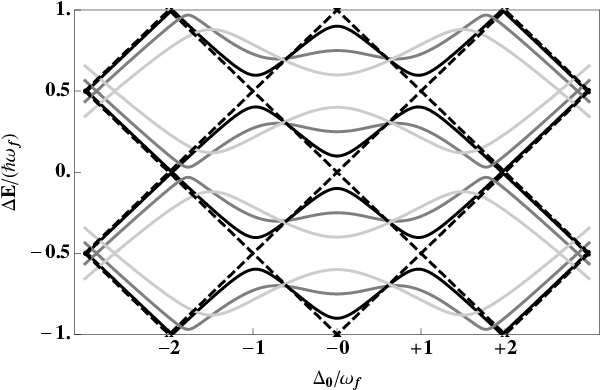
Figure 3 shows a generalisation of this energy level diagram, plotted as a function of $\Delta_{0}=\omega_{0}-j\omega_{f}$ along the horizontal axis. The nondegenerate basis states (dashed lines) $\ket{N,\tfrac 12}$ increase linearly with $\Delta_{0}$ while $\ket{N,-\tfrac 12}$ decrease linearly. These basis states cross whenever $\Delta_{0}/\omega_{f}$ takes an integer value. We label each crossing by this integer value, $q$. For $q=0$ the states $\ket{N,-\tfrac 12}$ and $\ket{N+j,\tfrac 12}$ are resonant as they are in Fig. 2. Generally the $q^{\mathrm{th}}$ resonance is between $\ket{N-\tfrac 12}$ and $\ket{N-(j+q),\tfrac 12}$.

The dressed levels (solid lines) are quite clearly forced apart for $q=-1,0,1$ predominantly due to the first order interactions with modes $j-1,\ j$ and $j+1$ respectively. The $q=\pm 1$ resonances are also shifted inwards slightly due to the level shift caused by second order interactions involving the off resonant modes. These shifts are the multi-frequency equivalent to the Bloch-Siegert shift. The contributing shifts to the $q=0$ resonance cancel when the amplitudes of modes $j\pm 1$ are balanced. Less prominent avoided crossings occur for $q=\pm 2$. These become noticeable as the field amplitudes increase (grey solid line) and are caused by resonant three photon interactions. Using our non-degenerate basis we are able to investigate these multi-frequency resonances and level shifts analytically in the section below.

We now derive effective Hamiltonians which describe the system near each of the crossings of the levels of $H_{0}$. For this we use the resolvent formalism, allowing us to account for the level shifts and interaction processes which couple these levels to an arbitrary precision.

Briefly, we introduce the formalism of the resolvent $G(z)=(z-H)^{-1}$ which is the advanced Green’s function for the Shroödinger equation. Its Fourier transform is the time evolution operator and we can interpret $G(z)$ as the propagator in the complex frequency ($z$) space. We are able to describe the dynamics between two energy states of $H_{0}$ (close to where they cross) using the projection of the resolvent $PG(z)P=(z-H_{\mathrm{eff}})^{-1}$ onto subspace $\mathscr{E}$ these states span. $H_{\mathrm{eff}}$ is the effective Hamiltonian between the two states and is given by

where $R(z)$ has the series expansion Cohen-Tannoudji et al. 1992

$P$ is the projection from $\mathscr{H}$ to $\mathscr{E}$ and $Q$ the projector onto its compliment $\bar{\mathscr{E}}$ and $G_{0}=(z-H_{0})^{-1}$ is the free propagator. The series expansion of $R(z)$ converges provided the energies within $\mathscr{E}$ are closer to each other than the energy of any state in $\bar{\mathscr{E}}$ with which they interact. Thus, the non-degenerate basis introduced in Sec. II is also necessary here to calculate multi-frequency effects using the resolvent formalism. The multi-frequency effects are encompassed by $R(z)$ where each term describes an interaction in $\mathscr{E}$ mediated via virtually excited states in $\bar{\mathscr{E}}$. These terms are easily evaluated analytically when the two states of interest are close to resonance with each other, but far from resonance with any other state, in which case $z$ is well approximated by their mean energy.

We interpret the effective Hamiltonian in powers of $V$. The terms of $H_{\mathrm{eff}}$ zeroth order in $V$ are merely the energies of the unperturbed levels of $H_{0}$. The first order terms in $V$ describe the direct interactions between states of $\mathscr{E}$. The second order terms, for the interaction discussed in this work, describe interactions which return to the same state they started, via an intermediate state in $\bar{\mathscr{E}}$. These self interactions shift the levels energy levels of $PH_{0}P$. Third order terms are between different initial and final states in $\mathscr{E}$ via two intermediate states in $\bar{\mathscr{E}}$.

To define the effective Hamiltonian at a given resonance we must find the relevant multi-photon processes which modify $PHP$. These processes, described generally by Eq. 17, are those that begin and end with states in $\mathscr{E}$ but have all intermediate states in $\bar{\mathscr{E}}$. Transitions between initial, intermediate and final states can only be those driven by the field modes present. Provided the Rabi frequencies are smaller than $\omega_{f}$, the leading terms are those lowest order in $V$. For three frequencies the processes up to third order are shown diagramatically in Fig. 4 for the $q=0$ resonance. The term for each multi-photon process is evaluated from matrix elements of individual transitions involved using Eq. 13a and the free propagators ($G_{0}$) of the intermediate states. The later are known from the intermediate state energies evaluated using Eq. 15.

We calculate effective Hamiltonians up to third order in $V$, first for the three frequency example considered of Fig. 3, then more generally for a large number of evenly spaced off-resonant frequencies. For convenience we abbreviate the resonant states $\ket{N-(j+q),\tfrac 12}$ and $\ket{N, -\tfrac 12}$ to $\ket{a}$ and $\ket{b}$ respectively. All energies are expressed relative to the mean energy $E_{0}=(E_{a}+E_{b})/2=\left[N-(j+q)/2\right]\omega_{f}$ at the resonance under consideration.

We begin by looking at the crossing $q=0$, where the initial and final states are $\ket{a}=\ket{N-j,\tfrac 12}$ and $\ket{b}=\ket{N,-\tfrac 12}$. We evaluate Eq. 16 for the processes shown in Fig. 4. Up to first order

where $\Omega_{j}=g_{j}(\gamma_{N-j}/\gamma_{N})\alpha_{j}\approx g_{j}\alpha_{j}$. We have labelled $\Delta$ with the subscript $q=0$ to show which resonance this detuning is from. At this level of approximation the system behaves like it is coupled only by a single-frequency $j\omega_{f}$.

The second order term of $R(z)$, $PVQG_{0}(z)QVP$, shifts the energies of $\ket{a}$ and $\ket{b}$ due virtual excitation of the intermediate states $\ket{N\pm 1,-\tfrac 12}$ and $\ket{N-j\pm, \tfrac 12}$ respectively. Thus, at second order the diagonal elements of Eq. 18 are shifted by

where $z$ can be approximated by zero. The resonance is therefore shifted to $\Delta_{0}=R_{bb}^{(2)}(0)-R_{aa}^{(2)}(0)$. However, when the amplitudes of the modes $j\pm 1$ are equal the two terms which contribute to each shift cancel to zero when $\Delta_{j}=0$, so in this case the resonance is unchanged.

The third order contribution modifies the interaction between $\ket{a}$ and $\ket{b}$, coupling them additionally via two intermediate states $\ket{N-j+1,\tfrac 12}$ and $\ket{N+1,-\tfrac 12}$ or $\ket{N-j-1,\tfrac 12}$ and $\ket{N-1,-\tfrac 12}$. The matrix elements for these terms are

and its Hermitian conjugate. At resonance, this third order interaction increases the splitting between $E_{a}$ and $E_{b}$ further than the value $\Omega_{j}$ expected for a single-frequency field.

The same approach can be adopted for the resonances $q=\pm 1$ with similar results. To lowest order the matrix elements are $\pm\tfrac{1}{2}\Delta_{q}$, where $\Delta_{q}=\omega_{0}-(j+q)\omega_{f}$. The first order contribution to the interaction matrix elements are $\tfrac{1}{2}\Omega_{j+q}$ and its Hermitian conjugate. The result Eq. 19a for the leading order level shift at $q=0$ can be generalised to

which not only applies to the cases $q=\pm 1$ but for any $q$. Unlike the $q=0$ case, these level shifts do not cancel on resonance. For $q=1$ these terms shift the resonance to negative value of $\Delta_{j+1}$, while for $q=-1$ the shift is to a positive value of $\Delta_{j-1}$.

For level crossings where $\absolutevalue{q}>1$ there is no direct coupling between the states $\ket{a}$ and $\ket{b}$ within the resonant subspace $\mathscr{E}$. For $q=\pm 2$ or $q=\pm 3$ the resonant states are only coupled by third and higher order processes. In general we find that at the $q^{\mathrm{th}}$ resonance, between states $\ket{a}=\ket{N-(j+q),\tfrac 12}$ and $\ket{b}=\ket{N,-\tfrac 12}$, the lowest order interaction is of order $q$ in $V$ when $q$ is odd, and of order $q+1$ when $q$ is even. For odd $q$ the effective interaction matrix element between the resonant states is

On resonance ($\Delta_{q}=0$), and approximating $z$ with zero, this effective interaction matrix element simplifies to

This shows the multi-photon resonant interaction strength scales generally as

with a characteristic Rabi frequency $\Omega\sim\Omega_{j}\forall j$.

For even $q$ there are $q+1$ different processes which contribute to the interaction matrix element, each of order $q+1$ in $V$. While the interaction processes are more numerous for even $q$ resonances, the coupling is typically weaker than that for $q-1$ unless the number of processes exceeds the relevant ratio $\Omega/\Delta$. Due to the multiple processes involved, the lowest order multi-photon matrix element for even $q$ is given by the more complicated expression

This expression is greatly simplified when applied to an individual resonance. For example the third order interaction for $q=2$ has

with $z\approx 0$. On resonance this simplifies to $\Omega_{j}\Omega_{j-1}^{*}\Omega_{j+1}/4$.

The effective Hamiltonian for each two dimensional subspace is easily solved to find the dressed states and their energies, which in general are

Thus the effective Rabi splitting at the multiphoton resonances is $2R_{ab}$. An atom, initially in its ground state therefore undergo Rabi oscillations

where $\Omega_{\mathrm{eff}}=2R_{ab}$ and $\widetilde{\Omega}_{\mathrm{eff}}=\sqrt{\left[\Delta_{q}-(R_{bb}-R_{aa})\right]^{2}+\Omega_{\mathrm{eff}}^{2}}$. Figure 5a shows the dressed energies calculated in this way agree well with the numerical approach given in Sec. III. Figure 5b shows the Rabi oscillations of this two-level subsystem calculated from the square modulus of Eq. 27, and for comparison, the same result calculated numerically. As $\Omega_{k}$ decrease the analytic approximation becomes more accurate. For larger $\Omega_{k}$ there is a leakage of the population to states outside the subspace considered, which is accounted for in the numerical results. In other work, we find simple analytic expression which accurately describe the time evolution in this case Yuen 2018.

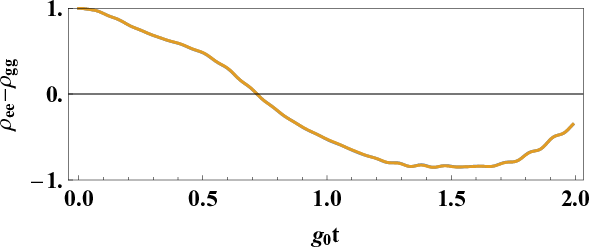
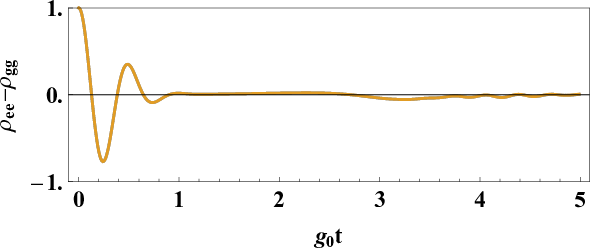
The electromagnetic fields considered here are in a product of coherent-states, which are the quantum states closest to coherent classical fields. We know however, that they differ from classical fields, and this differenced is most pronounced for weak fields where the mean photon number in each mode is small $\absolutevalue{\alpha_k}\sim 1$. For a single-frequency interacting with a spin-half system, a collapse of the Rabi oscillations is observed due dependence on the interaction strength on the square root of the photon number. Some time later revivals occur, but never complete since the frequency with which different pairs of atom-photon states oscillate is irrationally related Eberly et al. 1980. Thus, collapse and revivals are one hallmark of a quantised coherent field. We investigate the limits in which our non-degenerate theory accurately encapsulates the collapse of Rabi oscillations. Remarkably, we find that the our theory accurately predicts the collapse in the deep strong coupling regime in addition to the limit where the coherent fields are highly excited.

When multiple frequencies are present additional mechanisms effect the process of collapse. Additional frequencies change how the different components of oscillating spin-field system dephase. When additional frequencies are far from resonance compares to the interaction strength they drive virtual excitations which shift and the resonantly interacting levels providing further dephasing. When the interaction strength becomes comparable to the detuning between the field modes, the spin system is driven by many modes without any single mode dominating its dynamics. In turn the different modes of the field become entangled via the spin. As the interaction strength is increase beyond the mode spacing the multiple modes start to drive the spin collectively, each acting in a similar way.

To investigate the multi-mode dynamics and validate our theoretical formalism we calculate the time evolution for the multi-mode Rabi model numerically, both in the Fock basis and our non-degenerate basis, and compare the time evolution of the spin inversion $\rho_{ee}-\rho_{gg}$. The multimode Rabi model considered is

with coupling strength $g_{i}=\sqrt{\omega_{i}/\omega_{0}}g_{0}$, and $\omega_{0}$ is the lowest field frequency which we set resonant spin. Thus the coupling strength grows with $\sqrt{\omega}$ as is the case for the electromagnetic field, and is parameterised by $g_{0}$. We calculate $\ket{\psi(t)}$ for fields with two three frequencies with mode space $\Delta=1$ in dimensionless units. The initial state is a product of coherent-states, each with equal amplitude $\alpha$, with spin up. We compare $\rho_{ee}-\rho_{gg}$ calculated in the Fock and non-degenerate bases for a range of $g_{0},\omega_{0}$ and $\alpha$. We quantify the comparison between results in each basis using the $L_{2}$ measure

This integral is over the interval $t=0$ to $t=1/g$ - the characteristic time of the collapse for single-frequency Rabi oscillations Puri and Agarwal 1986.

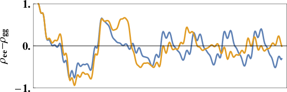
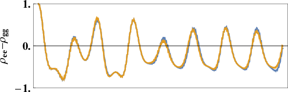
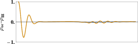
Figure 7 compares the spin population inversion calculated in the Fock and non-degenerate basis over a range of field amplitudes $\alpha$, coupling strengths $g_{0}$, and field frequencies $\bar{\omega}_{0}=\omega_{0}+\Delta/2$. Figure 6 shows typical population inversions for different $\alpha$ and $\omega_{0}$ with $g_{0}=\bar{\omega}/10$ in figures (a) to (c)), and different $g_{0}=\bar{\omega}$ and $\omega_{0}$ with $\absolutevalue{\alpha}=5$ in figures (d) to (f). In all cases there there is close agreement between Fock and non-degenerate basis calculations for times $g_{0}t\ll 1$. When $\bar{\omega}\sim 1$, $\alpha\sim 1$ and $g0/\bar{\omega}_{0}\sim 10^{-1}$ (ultra strong coupling), we find the results are quite different already by $g_{0}t\sim 1$. Typical examples are shown in Fig. 6a and 6b. We refer to this region of parameter space as region I, and the region outside this as region II. The level of agreement is quantified by their $L_{2}$ measure which is plotted in Fig. 7 and the boundary between regions I and II is indicated by the contour $L_{2}=10^{-3}$. For parameters in region II, the agreement becomes remarkably good even for longer times. Figures 6c, 6d, 6e and 6f show the population inversion typical of region II.

The strongest discrepancy between the Fock and non-degenerate basis calculations is for small $\omega_{0}$ where it is comparable to the frequency difference $\Delta$, small $g_{0}/\Delta$, and mean photon numbers $\absolutevalue{\alpha}\sim 1$. This arises because the non-degenerate basis does not cover Fock space since it represents many non-degenerate Fock states by a single state. The action of the field operators on this state is derived from the action on each underlying Fock state together with the set of amplitudes with which each contributes to the non-degenerate state. The action is correct provided that the field remains in a coherent-state. Gradually, the Fock states which contribute to a non-degenerate state will dephase. The rate of dephasing will be most significant when both field modes interact strongly with the spin but the two modes remain distinct such that their dynamics are different.

When the dephasing between components of the non-degenerate states is slow the non-degenerate basis yields accurate results. This is the case when $g_{0}$ becomes much larger than the mode spacing such that the difference in detuning between the spin and field modes becomes irrelevent. The dephasing is also slows as $\bar{\omega}_{0}$ increase for fixed $\Delta$. A perturbative expansion of the interaction shows that there are fewer low order processes which resonantly couple multi-mode Fock states when their frequencies approach.

In the limit of large photon number $\bar{n}\gg 1$ it is common to ignore the $n$-dependence of the interaction between different Fock states since its variance $\mathrm{var}(n)=\sqrt{\bar{n}}\ll\bar{n}$. While this is widely accepted, its universal application is limited to short times much shorted than $1/g_{0}$ - the timescale of Rabi oscillation collapse and is caused by the $n$-dependence of interactions. For multiple frequencies we give a similar approximation where the ratios $\gamma_{N}/\gamma_{N\pm k}$ are ignored, the variance of $N$ for this approximation being $\sigma_{N}$ and not $\sqrt{N}$. Figure 7a suggests that on a timescale $1/g_{0}$ the non-degenerate basis is remains suitable for accurate estimation of the spin population in the limit of large $\bar{N}$, but that this limit is approached slowly, compared with the increase in accuracy of the non-degenerate basis calculations for increasing frequency or coupling strength.

The comparison between the spin-dynamics calculated in the Fock and non-degenerate bases highlight two distinct regimes of multi-frequency light-matter interactions with coherent fields. Regime I: For weak fields and small $g_{0}/\Delta$ the dephasing between degenerate Fock states becomes important and leads to entanglement between the field modes via the spin. Regime II: For strong fields, or for weak fields and large $g_{0}/\Delta$, each mode remains in a coherent-state, and although the field and spin become entangled, the entanglement between modes is negligible. In the later regime, the dynamics of the field can be accurately represented in the non-degenerate basis. The semi-classical limit applies only for short times compared to $1/g_{0}$. The quantum dynamics then emerge for longer times, in one of these two regimes. In regime I the entanglement between the modes require a full quantum picture. Regime II lies between the quantum and classical limits, whereby its dynamics depend on the level of excitation of the field, but the field remains factorizable.

We have developed a formalism which tackles the complexity of multi-frequency atom-photon interactions when each field mode is well described by a coherent-state. We demonstrate its utility for strong strong fields and remarkably, for a wide range of parameters for weak fields where the quantum mechanical nature of the dynamics are important.

This formalism utilises a subspace of Fock space, spanned by a non-degenerate basis. This basis addresses the issue of level degeneracy encountered when working in the Fock basis. We have derived the effect of the photon creation and annihilation operators on these basis states including the asymmetry between them associated with quantum fluctuations. For highly excited coherent-states, where the photon number in each mode is large compared to unity, we show these fluctuations are small and can be ignored. We have demonstrated that by working in this basis, accurate calculations of the multi-frequency dressed states can be performed. Applying the resolvent formalism in this basis we have derived effective Hamiltonians which includes analytic expression for the level shifts and multi-photon interactions for an atom in a multi-frequency field.

For weak fields, where quantum effects are significant, we have compared the long time dynamics predicted by our formalism to exact calculations in the Fock basis. By investigating the parameter range for which our formalism is applicable we have identified two different quantum regimes for the collapse and revival of Rabi oscillations of a spin-half system in a multi-frequency field. One of these covers a large region in parameter space where some quantum aspects of the field are essential for the collapse, but the fields do not become entangled. Our formalism is uniquely capable of addressing problems in this regime.