Attribute-Driven Spontaneous Motion in Unpaired Image Translation
Abstract
Current image translation methods, albeit effective to produce high-quality results in various applications, still do not consider much geometric transform. We in this paper propose the spontaneous motion estimation module, along with a refinement part, to learn attribute-driven deformation between source and target domains. Extensive experiments and visualization demonstrate effectiveness of these modules. We achieve promising results in unpaired-image translation tasks, and enable interesting applications based on spontaneous motion.
1 Introduction
High-quality image generation is a fascinating task and has gained much attention in computer vision community. There has been great progress using generative adversarial networks (GAN) [9, 32]. Image translation, which produces modified images in target domain based on a given input from source domain, has been widely used in applications of style transfer [22], sketch/photo conversion [3, 15], label-based image synthesis [31], face editing [39] etc. Recent research trends continuously towards high practicality, e.g., images in high resolutions [36], and unpaired image translation [42], or using better latent space for more effective control [13, 21].
 |
 |
 |
| (a) Input | (b) StarGAN [4] | (c) CycleGAN [42] |
 |
 |
 |
| (d) MUNIT [8] | (e) Ours (SPM) | (f) Ours (SPM + R) |
Image translation mostly imposes the requirement of aligned or similar domains for texture or appearance transform. For example, in style transfer, the output image generally shares the same content with input. The building blocks of these networks, such as convolution/deconvolution layers and activation functions, are spatially corresponding. As shown in Fig. 1(a)-(d), visual artifacts, such as ghosting, could appear when nonsmile and smile faces are not geometrically aligned in image space.
In this paper, we take advantage of geometric correspondence in appearance transform. Taking the smiling face as an example in Fig. 1(e)-(f), decent results can be produced by applying geometric transform only, and they are better when a small refinement network follows. This architecture can greatly reduce visual artifacts mentioned above. This paper tackles the following three issues.
Single Image Deformation
Although several previous methods [37, 40, 35] employ various flow/warping/deformation by estimating motion, they are different from what we need in two aspects. First, traditional motion field estimation requires a pair of images to construct dense pixel correspondence, while in our task only one image is available. Second, motion fields for deformation are conditioned by examples, where one input image may need various motion constrained by target examples.
Different from all these settings, our goal is more like estimation of natural tendency of input images. We term it spontaneous motion (SPM) to distinguish from ordinary optical flow. This new tool adds a new dimension to image translation by introducing unpaired geometric transform. It also enables new ways of visualization, and finds interesting applications (described in Sec. 4.1). For example, in our framework, SPM for different target domains can be viewed as motion basis (Fig. 5), and linearly combining SPM basis enables convenient geometric edit (Fig. 13).
High Ill-posedness
Our framework is trained with neither paired data nor ground-truth motion field across domains. Cycle reconstruction loss and learning common latent space were considered to deal with unpaired data [42, 24]. Our geometric transform estimation across domains is even more ill-posed, since this set-to-set motion is more ambiguous compared to image-to-image correspondence given no ground-truth motion. Our spontaneous motion module applies two domain classifiers for translation result generation and motion estimation.
Inevitable Errors
Estimated motion fields are inevitably with errors due to large prediction freedom, missing-motion area to be filled (teeth of smiling faces are area missing in non-smile faces), and fine texture requirement for high quality results. Our system has a refinement module to fix remaining visual artifacts with an attention mask to filter out unnecessary changes on original images.
Our contributions are as follows. 1) We propose an end-to-end unpaired image translation system considering geometric deformation. 2) A conditional spontaneous motion estimation module, along with domain classifiers and a refinement step, to boost performance. 3) Our new framework achieves promising results in image translation, especially for unaligned scenarios.
2 Related Work
Unpaired Image Translation
Several unsupervised image translation methods were proposed. By introducing cycle-consistency loss for reconstruction, methods of [42, 41, 18] train the translation network across two domains without paired data. They train two separate networks for bidirectional image generation between source and target domains. Methods of [4, 30] extend the framework by introducing additional conditions to generate images in multiple domains. Another stream of research [25, 24, 34, 38, 28] is based on the assumption that images in source and target domains share the same latent space and in [13, 21], style and content are disentangled to control generated image style. They successfully translate images across domains. Because geometric relationship between domains is not considered, data that is not aligned or structurally very different cannot be well dealt with.
Geometry-Aware Image Translation
There exists work to build geometric relationship during image translation/generation. In [8, 27], geometric inconsistency between domains is mitigated with designed discriminator or losses. We note the generators are still composed of convolution-based blocks, which limit the generation power. Methods of [6, 37, 7, 40] estimate correspondence between two images. Dong et al. [6] relied on human body parsing, while Geng et al. [7] generated dense correspondence based on face landmarks. Methods of [37, 40] directly learn dense correspondence between two images. For these methods, paired reference images are needed to train or test, which does not fit semantic-level set-to-set transformation. Cao et al. [1] added another network for landmark learning; it cannot be trained in an end-to-end manner.
Our method is different. We do not need reference images and our framework is designed in an end-to-end way. Besides, the estimated spontaneous motion is conditioned on source domain content and target domain attributes, which can achieve semantic-level geometric transformation and generation.
3 Proposed Method
Given an image in source domain and target domain indicator ( is the total number of attributes), e.g. smiling, angry, and surprising. Our goal is to generate a high-quality image with attribute while keeping the identity of . Our framework resembles previous generative models by iteratively training generator/discriminator networks. However, in order to better handle geometric transform, we incorporate two new modules in generator as spontaneous motion module (Sec. 3.1) and refinement module (Sec. 3.2). Two types of classifiers are proposed as new losses to facilitate training. We extend our framework to high-resolution image generation () with special designs (Sec. 3.3). Our overall framework is depicted in Fig. 2. We elaborate on each module in the following.
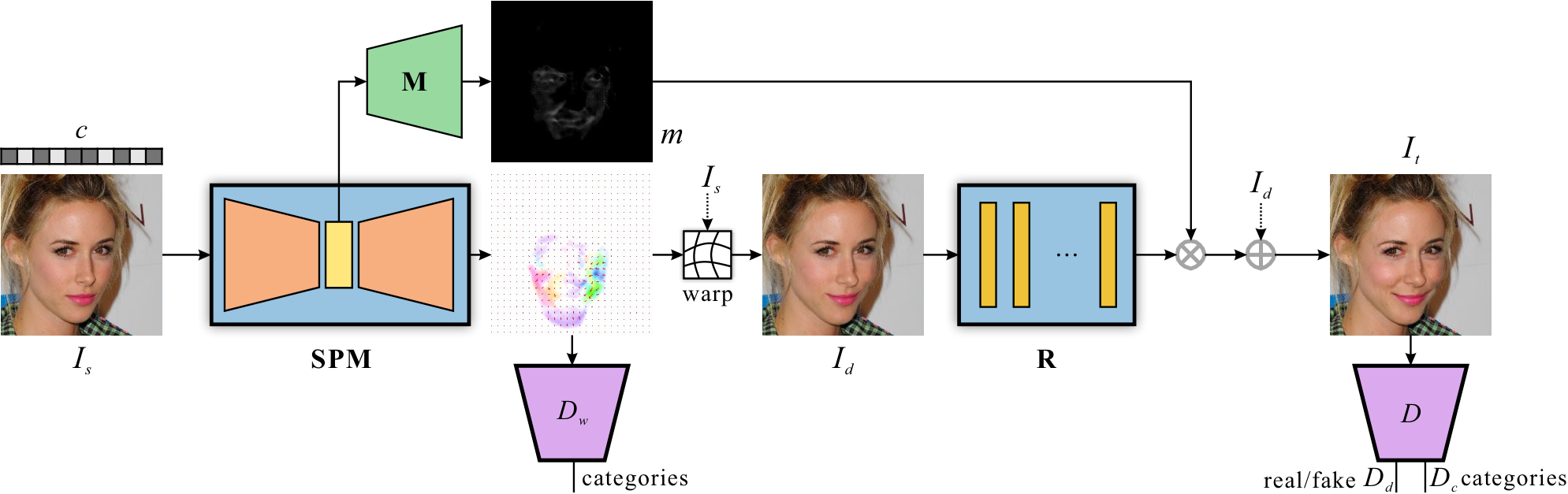
3.1 Spontaneous Motion Module
According to the analysis in Sec. 1, our spontaneous motion module aims to predict motion field based on input image and target indicator . We use an encoder-decoder network structure for its powerful fitting ability. For the design of this module, we consider the following facts.
Motion Field Decoding
In conventional image regression problems [14, 35, 5], activation functions in the final layer is usually not applied, in order to leave the output unbounded. This is because ground-truth pixel values are always in range , which supervise and prevent network output from divergence. In our motion estimation task, contrarily the output motion values can be largely varied, and the network can only be trained under indirect supervision, making convergence an issue, as verified in our experiments.
In order to mitigate this problem, we utilize as the last activation function to limit output in rather than . Moreover, we introduce an empirical multiplier to get the final . This seemingly tricky coefficient is actually quite reasonable in many tasks, such as face editing, since only local deformation is needed. In our paper, we set to for different datasets. Visualization of our estimated motion field with different targets is given in Fig. 5.
Motion Field Direction
To deform input to the target image, backward motion is usually considered as a vector from the target to source points [14, 6, 33]. However, such motion representation may not be suitable for convolution/deconvolution layer networks with aligned operators, since the representation is aligned to the unknown deformed image rather than the input one. Forward motion can mitigate the problem to some extent due to the alignment between input and forward motion. But deforming with forward warping may bring holes and more artifacts than with the backward one.
We experiment with these two solutions and adopt backward motion representation for deforming, because its result contains less artifacts and is more stable. Denoting image coordinates as , the set of valid image coordinates as , input image as , deformed image as and motion field as , we formulate the deformation step with bilinear interpolation as
| (1) |
where is bilinear interpolation operator.
As for the network structure of spontaneous motion module, we construct the encoder with 3 stride-2 convolution layers (each followed by instance normalization and ReLU) and 6 residual blocks to extract down-sampled feature map . A decoder then processes and up-samples by 3 deconvolution layers to a 2-channel motion field with the same size as the input image. In addition, high-level feature is utilized for attention mask learning, which will be described in Sec. 3.2.
To generate different dense motion fields for target indicators, we design two classifiers as constraints for both generation results and motion field estimation.
Domain Classifiers
We design image and motion domain classifiers in training. For image classifier , like that of [4], we add on top of discriminator as a constraint to classify the generated images into target domain . During training on , real image and its attribute are utilized to train with loss . At the stage of training generator , is fixed and the classification loss of generated images is utilized to optimize . The losses and are defined as
| (2) |
| (3) |
Although the classifier for generation results can guide the prediction of motion, we note a constraint on motion helps it more directly and better – motion fields for one domain (such as a face expression exemplified later in Fig. 5) have common features. It does not vary much even with different input images. With this observation, we design a classifier for motion fields, which classifies different motion fields into categories according to the target condition. It makes motion under different conditions share similar patterns and thus reduces bias or noise in generation steps. The classification loss for this classifier is formulated as
| (4) |
3.2 Refinement Module
The deformed image is further refined to reduce artifacts and enhance textural details. Specifically, two components are used.
Refinement with Residual Learning
We employ a refinement sub-network after deforming image . Instead of directly learning in images space, we learn the residual between deformed image and the unknown target, i.e. , since to learn residual for a well deformed image is easier and more reliable. As for the network structure, residual blocks [10] are sequentially concatenated without any downsample operation. The residual blocks are used for finer structure update. Thus we do not shrink images spatially, and instead take multiple stacked residual blocks to ensure final effect. In our experiments, we set to balance performance and efficiency.
Attention Mask
In image translation, generally only essential regions need to be updated (e.g. only mouth and its surrounding are changed when transforming neutral faces to smiling ones). We propose learning an attention mask , which marks important regions. The results are denoted as .
Specifically, as mentioned in Sec. 3.1, we obtain down-sampled feature map in module . catches high-level semantic information. We utilize it for attention mask learning. We build the attention mask module with 3 deconvolutional layers to up-sample into a 1-channel mask , the same size as the input. layer is used as the final activation layer to range the output mask in .
Directly learning an attention mask without any additional constraints is difficult, due to possible trivial solution of a mask with all-region selected. To avoid this problem, we introduce a regularization term to enforce sparsity of masks in -norm:
| (5) |
where , and are channel number, height and width of the mask respectively. The loss forces the attention mask to focus on the most important region.
3.3 Higher Resolution
To generate high resolution (HR) image by a single generator is difficult. Previous work [16, 23, 17] adopted coarse-to-fine or multi-stage training strategies. By incorporating motion estimation and refinement modules, we extend previous coarse-to-fine strategies to a pipeline with extra priors.
Priors and Adaptation
Previous coarse-to-fine strategies are usually applied to final output, i.e. using generated low-res (LR) images to guide HR generation. In our framework, we have more useful clues from LR, i.e. motion field for deformation, residual for refinement, mask for attention in low-resolution form. We utilize them to facilitate HR result generation.
We first train our initial framework with LR images until convergence. For higher resolution results, we feed in HR image and start from the well-trained LR framework while the weight of LR model is updated simultaneously in this stage. After obtaining motion field , residual , attention mask from LR generator with down-sampled from , we up-sample them to produce coarse results, i.e. , and with the same size as HR images . We further incorporate three light-weighted enhancement networks (, and ) respectively, each only contains two convolutional layers and a residual block. Finally, we estimate motion field as
| (6) |
Bilinear upsampling is used with the same process to obtain residual and attention mask . With these intermediate results, we deform by to get and then refine to yield final output .
Resolution Adaptive Discriminator
During training, the discriminators are designed as follows. In the LR-image training stage, we only train the LR image discriminator . We set real image as the positive sample while the generated is the negative one. In the HR image training stage, for , we have down-sampled as the positive sample and generated LR image as the negative one. Besides, we down-sample generated HR image to LR and feed them to as another type of negative samples. As for , and final generation result are positive and negative samples respectively. share similar network structure as , and yet with more convolution layers.
3.4 Other Loss Functions
Adversarial Loss
Ordinary generative adversarial loss is set for and formulated as
| (7) |
Reconstruction Loss
Total Loss
The final loss function for generator is
| (9) |
The loss function for is
| (10) |
In our experiments, we set , , and all to 1.0, and set and to 10.0 and 0.5 respectively.
4 Experiments
We conduct experiments on both CelebA [26] and RaFD [20]. CelebA contains 200K celebrity images and 40 attributes for each image with resolution . We utilize CelebA-HQ [16] in resolution for high-res image usage. To demonstrate the effectiveness of our framework, we select attributes with geometric deformation, i.e. ‘Smiling’, ‘Arched_eyebrow’, ‘Big_Nose’, and ‘Pointy_nose’ as condition to train our framework. RaFD is a smaller dataset with 67 identities, each displaying 8 emotional expressions, 3 gaze directions and 5 camera angles. We only train on frontal faces for robustness.
We implement the system on PyTorch [29] and run it on a TITAN Xp card. During our two-stage training, we first train on LR framework with images and batch size 16 for iterations. Then we train our extended network on higher resolutions or with batch size 8 for another iterations. We use Adam [19] with learning rate 1e-4 to optimize our framework.
4.1 Analysis
Effectiveness of SPM Module
We first visualize learned SPM. We experiment with an extreme case to learn image translation between a set of squares and circles. The position, color and size are random. The results in Fig. 3 demonstrate that our SPM module produces reasonable shapes. Remaining visual artifacts are further reduced by the refinement module.
 |
 |
 |
 |
 |
 |
 |
 |
| Input | Ground Truth |
Roles of Different Modules
For the spontaneous motion module, we aim to generate reasonable geometric movement, e.g. lips stretched for smiling faces. For the refinement module, it further suppresses noise and adds more texture on deformation results to make images look more realistic. A few intermediate and final ‘smiling’ results produced from these modules under different resolutions ( to ) are shown in Fig. 6. Effects from these two stages are clearly and respectively demonstrated.
Besides, to further study the roles of different modules, we train our framework with no spontaneous motion module (No_M) and no refinement module (No_R) respectively to see how results are altered. We show results in Fig. 4 and the quantitative comparison in Tab. 1. Without motion estimation, the geometric shape of images are wrong. The effect is like pasting patterns from the target domain to specific regions. Without the final refinement, results may contain distortions (right face in the 1st example) and artifacts (nose in the 2nd sample). Images also lack details to be a smiling face.
These experiments manifest the usefulness of both modules and our framework leverages their advantages.
 |
 |
 |
 |
 |
 |
 |
 |
| Input | No_M | No_R | Full |
SPM Field in Different Conditions
Motion patterns for the same face expression are generally similar even with different input images. For example, non-smiling to smiling faces need to ‘stretch’ pixels of lips. Taking the RaFD dataset as an example, motion fields for different emotions are visualized in Fig. 5. They tell different parts of faces required to be updated to achieve ideal facial expression.
 |
 |
 |
 |
 |
 |
 |
 |
 |
 |
 |
 |
 |
 |
 |
 |
 |
 |
 |
 |
 |
 |
 |
 |
| Input | Angry | Contemptuous | Disgusted | Fearful | Happy | Sad | Surprised |
 |
 |
 |
 |
 |
 |
 |
 |
 |
 |
 |
 |
| Input |
 |
 |
 |
 |
 |
 | |
 |
 |
 |
 |
 |
 |
 |
| Input |


Spontaneous Motion Field Basis Combination
Transformation varies when applying different motions to the same image. Since motion fields are independent, we can combine motion fields with simple addition operations. By adding differently learned motion fields, we achieve rough expression combination without re-training the network, under the condition that the combined transformation does not conflict with each other. We demonstrate the effect of combination in Fig. 13. The difference in generated micro-expression is very useful for fine face attribute creation.
4.2 Comparisons
We compare with several prevalent methods in image translation. They are StarGAN [4], CycleGAN [42], MUNIT [13] and Ganimorph [8]. StarGAN [4] is the first framework for multi-condition image translation. CycleGAN [42] and MUNIT [13] are important methods in image translation. Ganimorph [8] is a geometry-aware framework based on CycleGAN [42], which is another solution to geometric transformation across domains in image translation.
4.2.1 Visual Comparison
We conduct experiments on the two datasets for comparative evaluation. On the CelebA dataset, we treat each attribute transformation as a two-domain translation from non- to . Fig. 8 shows that CycleGAN, MUNIT, and Ganimorph cannot capture domain information when the attribute transformation is subtle, like ‘Big_Nose’ and ‘Pointy_Nose’. They tend to reconstruct the input image instead. Both StarGAN and our method handle such subtle domain translation thanks to the domain classifiers.
Our method better tackles geometry variation and image misalignment. For other attributes like ‘smiling’, though all previous methods transform source images to target domain, various types of geometric deformation lead to quality difference on results, causing noticeable ghosting or artifacts. Our method, contrarily, alleviates this issue.
For the RaFD dataset (Fig. 9), similarly, StarGAN handles domain transformation and yet are with room to improve details and geometric shapes, especially for the ‘happy’ expression. Our framework satisfies target conditions better thanks to our explicit spontaneous motion module and our two domain classifiers for training.
|
StarGAN |
 |
 |
 |
 |
 |
 |
 |
 |
|---|---|---|---|---|---|---|---|---|
|
CycleGAN |
|
 |
 |
 |
 |
 |
 |
 |
|
Ganimorph |
|
 |
 |
 |
 |
 |
 |
 |
|
Ours |
|
 |
 |
 |
 |
 |
 |
 |
| Input | Angry | Contemptuous | Disgusted | Fearful | Happy | Sad | Surprised |
4.2.2 Quantitative Comparison
Distribution Discrepancy
To evaluate generated faces quantitatively, we extract features with a deep face feature extractor VGGFace2 [2] and use FID [12] to measure feature distribution discrepancy between real and generated faces. For each attribute, we first extract feature from real faces with such an attribute in test set, and then extract features from translated images (to this attribute) by each method to be compared.
We calculate FID between and for each method. Results in Tab. 1 demonstrate that our framework achieves the lowest FID score among all methods, which indicates that the feature distribution of our generated images is closest to that of real images.
| Methods / () | S | BN | PN | AE | Acc.(%) |
|---|---|---|---|---|---|
| StarGAN | 3.676 | 7.875 | 6.933 | 3.751 | 95.67 |
| CycleGAN | 4.011 | 5.262 | 4.886 | 4.171 | 91.23 |
| Ganimorph | 4.689 | 5.645 | 5.129 | 5.570 | 86.25 |
| MUNIT | 5.189 | 5.551 | 4.761 | 5.271 | 81.43 |
| Ours (No_M) | 3.224 | 6.051 | 5.682 | 4.667 | 88.29 |
| Ours (No_R) | 3.022 | 6.505 | 5.894 | 3.911 | 90.96 |
| Ours (Full) | 2.907 | 5.137 | 4.704 | 3.678 | 97.85 |
| Real | - | - | - | - | 98.75 |
Classification Accuracy
Following [4], we compute the classification accuracy of facial expression on generated images. We first train a facial expression classifier with ResNet-18 [11] on the RaFD dataset with the train set. We achieve near-perfect accuracy of 98.75% on test set. Then we apply this well-trained classifier to compute classification accuracy on synthesized images output from different methods. The results in Table 1 indicate that we achieve the best results in terms of classification accuracy. StarGAN works also very well benefited by its domain classification framework.
4.2.3 User Study
We also conduct user study for method comparison among 101 subjects, with 21 groups of generated samples. Given an input image, subjects are instructed to choose the best item based on quality of attribute transfer, perceptual realism, and preservation of identity. The results in Table 2 demonstrate that our method performs best among different facial attribute transformation methods, while StarGAN [4] performs well for subtle facial attribute (e.g. Big_Nose) transformation and CycleGAN [42] yields decent output on obvious attributes (e.g. Arched_Eyebrow, Smiling).
| Methods | S (%) | BN (%) | PN (%) | AE (%) |
|---|---|---|---|---|
| StarGAN | 10.17 | 25.66 | 16.83 | 24.24 |
| CycleGAN | 14.41 | 8.85 | 14.85 | 28.79 |
| Ganimorph | 5.93 | 5.31 | 6.93 | 1.52 |
| MUNIT | 11.44 | 7.96 | 11.88 | 3.03 |
| Ours | 58.05 | 52.21 | 49.50 | 42.42 |
5 Conclusion
In this paper, we have introduced geometric deformation into image translation frameworks. We proposed spontaneous motion estimation module followed by refinement to fix remaining artifacts in deformation results. Extensive experiments manifest the effectiveness of our proposed framework. It achieves promising results for image translation and enables new visualization and applications. Our method may also shed lights on geometric-aware image translation.
References
- [1] Kaidi Cao, Jing Liao, and Lu Yuan. Carigans: Unpaired photo-to-caricature translation, 2018.
- [2] Qiong Cao, Li Shen, Weidi Xie, Omkar M Parkhi, and Andrew Zisserman. Vggface2: A dataset for recognising faces across pose and age. In 2018 13th IEEE International Conference on Automatic Face & Gesture Recognition (FG 2018), 2018.
- [3] Wengling Chen and James Hays. Sketchygan: towards diverse and realistic sketch to image synthesis. In CVPR, 2018.
- [4] Yunjey Choi, Minje Choi, Munyoung Kim, Jung-Woo Ha, Sunghun Kim, and Jaegul Choo. Stargan: Unified generative adversarial networks for multi-domain image-to-image translation. In CVPR, 2018.
- [5] Chao Dong, Chen Change Loy, Kaiming He, and Xiaoou Tang. Learning a deep convolutional network for image super-resolution. In ECCV, 2014.
- [6] Haoye Dong, Xiaodan Liang, Ke Gong, Hanjiang Lai, Jia Zhu, and Jian Yin. Soft-gated warping-gan for pose-guided person image synthesis. In NeurIPS, 2018.
- [7] Jiahao Geng, Tianjia Shao, Youyi Zheng, Yanlin Weng, and Kun Zhou. Warp-guided gans for single-photo facial animation. In SIGGRAPH Asia 2018 Technical Papers, 2018.
- [8] Aaron Gokaslan, Vivek Ramanujan, Daniel Ritchie, Kwang In Kim, and James Tompkin. Improving shape deformation in unsupervised image-to-image translation. In ECCV, 2018.
- [9] Ian Goodfellow, Jean Pouget-Abadie, Mehdi Mirza, Bing Xu, David Warde-Farley, Sherjil Ozair, Aaron Courville, and Yoshua Bengio. Generative adversarial nets. In NeurIPS, 2014.
- [10] Kaiming He, Xiangyu Zhang, Shaoqing Ren, and Jian Sun. Deep residual learning for image recognition. In CVPR, 2016.
- [11] Kaiming He, Xiangyu Zhang, Shaoqing Ren, and Jian Sun. Deep residual learning for image recognition. In CVPR, 2016.
- [12] Martin Heusel, Hubert Ramsauer, Thomas Unterthiner, Bernhard Nessler, Günter Klambauer, and Sepp Hochreiter. Gans trained by a two time-scale update rule converge to a nash equilibrium. arXiv preprint arXiv:1706.08500, 2017.
- [13] Xun Huang, Ming-Yu Liu, Serge Belongie, and Jan Kautz. Multimodal unsupervised image-to-image translation. arXiv preprint arXiv:1804.04732, 2018.
- [14] Eddy Ilg, Nikolaus Mayer, Tonmoy Saikia, Margret Keuper, Alexey Dosovitskiy, and Thomas Brox. Flownet 2.0: Evolution of optical flow estimation with deep networks. In CVPR, 2017.
- [15] Phillip Isola, Jun-Yan Zhu, Tinghui Zhou, and Alexei A Efros. Image-to-image translation with conditional adversarial networks. CVPR, 2017.
- [16] Tero Karras, Timo Aila, Samuli Laine, and Jaakko Lehtinen. Progressive growing of gans for improved quality, stability, and variation. arXiv preprint arXiv:1710.10196, 2017.
- [17] Tero Karras, Samuli Laine, and Timo Aila. A style-based generator architecture for generative adversarial networks. arXiv preprint arXiv:1812.04948, 2018.
- [18] Taeksoo Kim, Moonsu Cha, Hyunsoo Kim, Jung Kwon Lee, and Jiwon Kim. Learning to discover cross-domain relations with generative adversarial networks. In ICML, 2017.
- [19] Diederik P Kingma and Jimmy Ba. Adam: A method for stochastic optimization. arXiv preprint arXiv:1412.6980, 2014.
- [20] Oliver Langner, Ron Dotsch, Gijsbert Bijlstra, Daniel HJ Wigboldus, Skyler T Hawk, and AD Van Knippenberg. Presentation and validation of the radboud faces database. Cognition and emotion, 2010.
- [21] Hsin-Ying Lee, Hung-Yu Tseng, Jia-Bin Huang, Maneesh Singh, and Ming-Hsuan Yang. Diverse image-to-image translation via disentangled representations. In ECCV, 2018.
- [22] Chuan Li and Michael Wand. Precomputed real-time texture synthesis with markovian generative adversarial networks. In ECCV, 2016.
- [23] Minjun Li, Haozhi Huang, Lin Ma, Wei Liu, Tong Zhang, and Yugang Jiang. Unsupervised image-to-image translation with stacked cycle-consistent adversarial networks. In ECCV, 2018.
- [24] Ming-Yu Liu, Thomas Breuel, and Jan Kautz. Unsupervised image-to-image translation networks. In NeurIPS, 2017.
- [25] Ming-Yu Liu and Oncel Tuzel. Coupled generative adversarial networks. In NeurIPS, 2016.
- [26] Ziwei Liu, Ping Luo, Xiaogang Wang, and Xiaoou Tang. Deep learning face attributes in the wild. In ICCV, 2015.
- [27] Roey Mechrez, Itamar Talmi, and Lihi Zelnik-Manor. The contextual loss for image transformation with non-aligned data. arXiv preprint arXiv:1803.02077, 2018.
- [28] Zak Murez, Soheil Kolouri, David Kriegman, Ravi Ramamoorthi, and Kyungnam Kim. Image to image translation for domain adaptation. arXiv preprint arXiv:1712.00479, 2017.
- [29] Adam Paszke, Sam Gross, Soumith Chintala, Gregory Chanan, Edward Yang, Zachary DeVito, Zeming Lin, Alban Desmaison, Luca Antiga, and Adam Lerer. Automatic differentiation in pytorch. In NIPS-W, 2017.
- [30] Albert Pumarola, Antonio Agudo, Aleix M Martinez, Alberto Sanfeliu, and Francesc Moreno-Noguer. Ganimation: Anatomically-aware facial animation from a single image. In ECCV, 2018.
- [31] Xiaojuan Qi, Qifeng Chen, Jiaya Jia, and Vladlen Koltun. Semi-parametric image synthesis. In CVPR, 2018.
- [32] Alec Radford, Luke Metz, and Soumith Chintala. Unsupervised representation learning with deep convolutional generative adversarial networks. arXiv preprint arXiv:1511.06434, 2015.
- [33] Aliaksandr Siarohin, Stéphane Lathuilière, Segey Tulyakov, Elisa Ricci, and Nicu Sebe. Animating arbitrary objects via deep motion transfer. arXiv preprint arXiv:1812.08861, 2018.
- [34] Yaniv Taigman, Adam Polyak, and Lior Wolf. Unsupervised cross-domain image generation. arXiv preprint arXiv:1611.02200, 2016.
- [35] Xin Tao, Hongyun Gao, Renjie Liao, Jue Wang, and Jiaya Jia. Detail-revealing deep video super-resolution. In ICCV, 2017.
- [36] Ting-Chun Wang, Ming-Yu Liu, Jun-Yan Zhu, Andrew Tao, Jan Kautz, and Bryan Catanzaro. High-resolution image synthesis and semantic manipulation with conditional gans. In CVPR, 2018.
- [37] Ziwei Liu Weidong Yin and Chen Change Loy. Instance level facial attributes transfer with geometry-aware flow. In AAAI, February 2019.
- [38] Lior Wolf, Yaniv Taigman, and Adam Polyak. Unsupervised creation of parameterized avatars. In ICCV, 2017.
- [39] Taihong Xiao, Jiapeng Hong, and Jinwen Ma. Elegant: Exchanging latent encodings with gan for transferring multiple face attributes. In ECCV, 2018.
- [40] Raymond A. Yeh, Ziwei Liu, Dan B Goldman, and Aseem Agarwala. Semantic facial expression editing using autoencoded flow. 2016.
- [41] Zili Yi, Hao (Richard) Zhang, Ping Tan, and Minglun Gong. Dualgan: Unsupervised dual learning for image-to-image translation. In ICCV, 2017.
- [42] Jun-Yan Zhu, Taesung Park, Phillip Isola, and Alexei A Efros. Unpaired image-to-image translation using cycle-consistent adversarial networks. In ICCV, 2017.
6 Appendix
6.1 More Discussions
6.1.1 Attention Mask Learning
We learn attention masks to filter out unnecessary noises and focus on essential regions during transformation. Taking the attribute (Smiling, Arched_eyebrow, Big_Nose) transforms in CelebA dataset as examples, the generated attention mask is shown in Fig. 10. We can see that for ‘Smiling’ transformation, the attention area is mouth, cheekbones and related region. ‘Arched_eyebrow’ transformation will focus on eyebrow region and ‘Big_Nose’ will focus on two sides of nose.
|
Smiling |
 |
 |
 |
 |
|---|---|---|---|---|
|
Eyebrow |
 |
 |
 |
 |
|
Nose |
 |
 |
 |
 |
6.1.2 Other Application
Face to Bitmoji
We also conduct experiments on other image translation applications to test the effectiveness of our framework. Specifically, we evaluate our framework in real face to bitmoji face application, since the two domains are quite different in both texture and geometric shape. The results are demonstrated in Fig. 11. From the results we can see that spontaneous motion module will firstly deform input faces to bitmoji faces in geometric shape (SPM), then the refinement module render the deformed results with bitmoji textures to get the final results (SPM + R). This working pipeline may effectively get rid of distortions and artifacts caused by current generators with all aligned operators (i.e. convolution / de-convolution layers).
 |
 |
 |
 |
 |
 |
 |
 |
 |
 |
 |
 |
 |
 |
 |
 |
 |
 |
 |
 |
| Input | StarGAN |
6.1.3 High Resolution Results
We demonstrate higher resolution, i.e. results in Fig. 12. All results with different resolutions in our paper start from generating images. To generate results, we adopt the training strategy on Sec 3.4 in our paper for one time, while we would up-sample twice with the same strategy for image generation.
 |
 |
 |
 |
 |
 |
 |
 |
 |
 |
 |
 |
 |
 |
 |
 |
 |
 |
 |
 |
| Input | Input |
6.1.4 More Combination Cases
More cases for combination of spontaneous motion basis are shown in Fig. 13. It produces the combination of different facial attributes.
 |
 |
 |
 |
 |
 | |
 |
 |
 |
 |
 |
 |
 |
 |
 |
 |
 |
 |
 | |
 |
 |
 |
 |
 |
 |
 |
 |
 |
 |
 |
 |
 | |
 |
 |
 |
 |
 |
 |
 |
 |
 |
 |
 |
 |
 | |
 |
 |
 |
 |
 |
 |
 |
| Input |
6.2 More Visual Results
More visual results with different facial attribute transforms are shown in Fig. 14 (CelebA dataset) and Fig. 15 (RaFD dataset).
 |
 |
 |
 |
 |
 |
 |
 |
 |
 |
 |
 |
 |
 |
 |
 |
|
|
 |
 |
 |
 |
 |
 |
(a) Arched_Eyebrow.
 |
 |
 |
 |
 |
 |
 |
 |
 |
 |
 |
 |
 |
 |
 |
 |
 |
 |
 |
 |
 |
 |
|
|
(b) Big_Nose.
 |
 |
 |
 |
 |
 |
 |
 |
 |
 |
 |
 |
 |
 |
 |
 |
 |
 |
 |
 |
 |
 |
 |
 |
(c) Pointy_Nose.
 |
 |
 |
 |
 |
 |
 |
 |
 |
 |
 |
 |
 |
 |
 |
 |
 |
 |
 |
 |
 |
 |
 |
 |
 |
 |
 |
 |
 |
 |
 |
 |
 |
 |
 |
 |
 |
 |
 |
 |
 |
 |
 |
 |
 |
 |
 |
 |
 |
 |
 |
 |
 |
 |
 |
 |
 |
 |
 |
 |
 |
 |
 |
 |
 |
 |
 |
 |
 |
 |
 |
 |
| Input | Angry | Contemptuous | Disgusted | Fearful | Happy | Sad | Surprised |
6.3 Network Architecture
We follow the design of [4] to set up our encoder-decoder structure for different modules of generator. The architecture detail of each module is illustrated as below.
For the layers demonstrated in Tab. 3, 4 & 5, “conv” and “deconv” indicate a convolution layer and a de-convolution layer respectively, each followed by an instance-normalization and a ReLU layer. Specifically, “conv_output” indicates a convolution layer without normalization or activation layer. Besides, “ResBlock” indicates residual blocks defined in [11], while the original batch-normalization layer is replaced by instance-normalization layer and means residual blocks are stacked.
Spontaneous Motion Module
Spontaneous motion module (SPM) is an image-attribute pair to motion field network, we construct the module with an encoder-decoder framework. The detail of network architecture is shown in Tab. 3.
| Layer | Output Size | (kernel, stride) |
|---|---|---|
| Inputs | (- , -) | |
| conv1 | (7, 1) | |
| conv2 | (4, 2) | |
| conv3 | (4, 2) | |
| ResBlock | (3, 1) | |
| deconv1 | (4, 2) | |
| deconv2 | (4, 2) | |
| conv_output | (7, 1) | |
| Tanh | (-, -) |
Attention Mask Module
Attention mask module (M) is utilized to focus on the essential part for refinement by predicting a mask in . The structure of M is a decoder, which takes extracted feature after ResBlocks from SPM as input and outputs a one-channel mask. The network detail of M is shown in Tab. 4.
| Layer | Output Size | (kernel, stride) |
|---|---|---|
| Inputs | (- , -) | |
| deconv1 | (4, 2) | |
| deconv2 | (4, 2) | |
| conv_output | (7, 1) | |
| Sigmoid | (-, -) |
Refinement Module
Refinement module R takes deformed image from SPM as input, and outputs the refined image by introducing residual blocks. R takes no down-sampling operation in order to keep the spatial information and refine the fine structure of deformed image. The network detail of R is shown in Tab. 5.
| Layer | Output Size | (kernel, stride) |
|---|---|---|
| Inputs | (- , -) | |
| conv1 | (7, 1) | |
| ResBlock | (3, 1) | |
| conv_output | (7, 1) | |
| Tanh | (-, -) |