Strategic Learning for Active, Adaptive, and Autonomous Cyber Defense
Abstract
The increasing instances of advanced attacks call for a new defense paradigm that is active, autonomous, and adaptive, named as the ‘3A’ defense paradigm. This chapter introduces three defense schemes that actively interact with attackers to increase the attack cost and gather threat information, i.e., defensive deception for detection and counter-deception, feedback-driven Moving Target Defense (MTD), and adaptive honeypot engagement. Due to the cyber deception, external noise, and the absent knowledge of the other players’ behaviors and goals, these schemes possess three progressive levels of information restrictions, i.e., from the parameter uncertainty, the payoff uncertainty, to the environmental uncertainty. To estimate the unknown and reduce the uncertainty, we adopt three different strategic learning schemes that fit the associated information restrictions. All three learning schemes share the same feedback structure of sensation, estimation, and actions so that the most rewarding policies get reinforced and converge to the optimal ones in autonomous and adaptive fashions. This work aims to shed lights on proactive defense strategies, lay a solid foundation for strategic learning under incomplete information, and quantify the tradeoff between the security and costs.
1 Introduction
Recent instances of WannaCry ransomware, Petya cyberattack, and Stuxnet malware have demonstrated the trends of modern attacks and the corresponding new security challenges as follows.
- •
Advanced: Attackers leverage sophisticated attack tools to invalidate the off-the-shelf defense schemes such as the firewall and intrusion detection systems.
- •
Targeted: Unlike automated probes, targeted attacks conduct thorough research in advance to expose the system architecture, valuable assets, and defense schemes.
- •
Persistent: Attackers can restrain the adversary’s behaviors and bide their times to launch critical attacks. They are persistent in achieving the goal.
- •
Adaptive: Attackers can learn the defense strategies and unpatched vulnerabilities during the interaction with the defender and tailor their strategies accordingly.
- •
Stealthy and Deceptive: Attackers conceal their true intentions and disguise their claws to evade detection. The adversarial cyber deception endows attackers an information advantage over the defender.
Thus, defenders are urged to adopt active, adaptive, and autonomous defense paradigms to deal with the above challenges and proactively protect the system prior to the attack damages rather than passively compensate for the loss. In analogy to the classical Kerckhoffs’s principle in the 19th century that attackers know the system, we suggest a new security principle for modern cyber systems as follows: {svgraybox} Principle of 3A Defense: A cyber defense paradigm is considered to be insufficiently secure if its effectiveness relies on
- •
Rule-abiding human behaviors.
- •
A perfect protection against vulnerabilities and a perfect prevention from system penetration.
- •
A perfect knowledge of attacks.
Firstly, of data breaches are caused by privilege misuse and error by insiders according to Verizon’s data breach report in Jeff2000. Security administration does not work well without the support of technology, and autonomous defense strategies are required to deal with the increasing volume of sophisticated attacks. Secondly, systems always have undiscovered vulnerabilities or unpatched vulnerabilities due to the long supply chain of uncontrollable equipment providers shackleford2015combatting and the increasing complexities in the system structure and functionality. Thus, an effective paradigm should assume a successful infiltration and pursue strategic securities through interacting with intelligent attackers. Finally, due to adversarial deception techniques and external noises, the defender cannot expect a perfect attack model with predicable behaviors. The defense mechanism should be robust under incomplete information and adaptive to the evolution of attacks.
In this chapter, we illustrate three active defense schemes in our previous works, which are designed based on the new cyber security principle. They are defensive deception for detection and counter-deception huang2019adaptive; huang2018analysis; APTjournal in Section 2, feedback-driven Moving Target Defense (MTD) zhu2013game in Section 3, and adaptive honeypot engagement huangHoneypot in Section 4. All three schemes is of incomplete information, and we arrange them based on three progressive levels of information restrictions as shown in the left part of Fig. 1.
t]

The first scheme in Section 2 considers the obfuscation of characteristics of known attacks and systems through a random parameter called the player’s type. The only uncertainty origins from the player’s type, and the mapping from the type to the utility is known deterministically. The MTD scheme in Section 3 considers unknown attacks and systems whose utilities are completely uncertain, while the honeypot engagement scheme in Section 4 further investigates environmental uncertainties such as the transition probability, the sojourn distribution, and the investigation reward.
To deal with these uncertainties caused by different information structures, we suggest three associated learning schemes as shown in the right part of Fig. 1, i.e., Bayesian learning for the parameter estimation, distributed learning for the utility acquisition without information sharing, and reinforcement learning for the optimal policy obtainment under the unknown environment. All three learning methods form a feedback loop that strategically incorporates the samples generated during the interaction between attackers and defenders to persistently update the beliefs of known and then take actions according to current optimal decision strategies. The feedback structure makes the learning adaptive to behavioral and environmental changes.
Another common point of these three schemes is the quantification of the tradeoff between security and the different types of cost. In particular, the costs result from the attacker’s identification of the defensive deception, the system usability, and the risk of attackers penetrating production systems from the honeynet, respectively.
1.1 Literature
The idea of using deceptions defensively to detect and deter attacks has been studied theoretically as listed in the taxonomic survey pawlick2017game, implemented to the Adversarial Tactics, Techniques and Common Knowledge (ATT&CKTM) adversary model system stech2016integrating, and tested in the real-time cyber-wargame experiment heckman2013active. Many previous works imply the similar idea of type obfuscation, e.g., creating social network avatars (fake personas) on the major social networks gomez2018r, implementing honey files for ransomware actions virvilis2014changing, and disguising a production system as a honeypot to scare attackers away pawlick2018modeling.
Moving target defense (MTD) allows dynamic security strategies to limit the exposure of vulnerabilities and the effectiveness of the attacker’s reconnaissance by increasing complexities and costs of attacks jajodia2011moving. To achieve an effective MTD, kc2003countering proposes the instruction set and the address space layout randomization, clark2012deceptive studies the deceptive routing against jamming in multi-hop relay networks, and maleki2016markov uses the Markov chain to model the MTD process and discusses the optimal strategy to balance the defensive benefit and the network service quality.
The previous two methods use the defensive deception to protect the system and assets. To further gather threat information, the defender can implement honeypots to lure attackers to conduct adversarial behaviors and reveal their TTPs in a controlled and monitored environment. Previous works hecker2012methodology; la2016deceptive have investigated the adaptive honeypot deployment to effectively engage attackers without their notices. The authors in recent work PawlickNZ17 proposes a continuous-state Markov Decision Process (MDP) model and focuses on the optimal timing of the attacker ejection.
Game-theoretic models are natural frameworks to capture the multistage interaction between attackers and defenders. Recently, game theory has been applied to different sets of security problems, e.g., Stackelberg and signaling games for deception and proactive defenses pawlick_stackelberg_2016; zhu2013game; zhu2013deployment; zhu2013hybrid; zhu2012interference; clark2012deceptive; zhu2012game; zhu2012deceptive; zhu2010stochastic, network games for cyber-physical security xu2017secure; xu_game-theoretic_2017; xu_cross-layer_2016; farooq2019modeling; xu2015cyber; huang2017large; chen2017dynamic; miao2018hybrid; yuan2013resilient; Rass&Zhu2016, dynamic games for adaptive defense zhu2010dynamic; zhang2017strategic; huang2018gamesec; huang2018PER; huang2019adaptive; pawlick2015flip; farhang2014dynamic; zhu2009dynamic; zhu2010network; zhu2010heterogeneous, and mechanism design theory for security chen_security_2017; zhang_bi-level_2017; zhang_attack-aware_2016; casey2015compliance; hayel2015attack; hayel2017epidemic; zhu2012guidex; zhu2012tragedy; zhu2009game.
Information asymmetry among the players in network security is a challenge to deal with. The information asymmetry can be either leveraged or created by the attacker or the defender for achieving a successful cyber deception. For example, techniques such as honeynets carroll2011game; zhu2013deployment, moving target defense zhu2013game; jajodia2011moving; huang2019adaptive, obfuscation pawlick2016stackelberg; zhang_dynamic_2017; farhang2015phy; zhang2018distributed, and mix networks zhang2010gpath have been introduced to create difficulties for attackers to map out the system information.
To overcome the created or inherent uncertainties of networks, many works have studied the strategic learning in security games, e.g., Bayesian learning for unknown adversarial strategies garnaev2015security, heterogeneous and hybrid distributed learning zhu2010heterogeneous; zhu2011distributed, multiagent reinforcement learning for intrusion detection servin2008multi. Moreover, these learning schemes are combined to achieve better properties, e.g., distributed Bayesian learning djuric2012distributed, Bayesian reinforcement learning chalkiadakis2003coordination, and distributed reinforcement learning chen2015distributed.
1.2 Notation
Throughout the chapter, we use calligraphic letter to define a set and as the cardinality of the set. Let represent the set of probability distributions over . If set is discrete and finite, , otherwise, . Row player is the defender (pronoun ‘she’) and (pronoun ‘he’) is the user (or the attacker) who controls the column of the game matrix. Both players want to maximize their own utilities. The indicator function equals one if , and zero if .
1.3 Organization of the Chapter
The rest of the paper is organized as follows. In Section 2, we elaborate defensive deception as a countermeasure of the adversarial deception under a multistage setting where Bayesian learning is applied for the parameter uncertainty. Section 3 introduces a multistage MTD framework and the uncertainties of payoffs result in distributed learning schemes. Section 4 further considers reinforcement learning for environmental uncertainties under the honeypot engagement scenario. The conclusion and discussion are presented in Section 5.
2 Bayesian Learning for Uncertain Parameters
Under the mild restrictive information structure, each player’ utility is completely governed by a finite group of parameters which form his/her type. Each player’s type characterizes all the uncertainties about this player during the game interaction, e.g., the physical outcome, the payoff function, and the strategy feasibility, as an equivalent utility uncertainty without loss of generality harsanyi1967games. Thus, the revelation of the type value directly results in a game of complete information. In the cyber security scenario, a discrete type can distinguish either systems with different kinds of vulnerabilities or attackers with different targets. The type can also be a continuous random variable representing either the threat level or the security awareness level huang2019adaptive; huang2018analysis. Since each player takes actions to maximize his/her own type-dependent utility, the other player can form a belief to estimate ’s type based on the observation of ’s action history. The utility optimization under the beliefs results in the Perfect Bayesian Nash Equilibrium (PBNE) which generates new action samples and updates the belief via the Bayesian rule. We plot the feedback Bayesian learning process in Fig. 2 and elaborate each element in the following subsections based on our previous work APTjournal.
t]

2.1 Type and Multistage Transition
Through adversarial deception techniques, attackers can disguise their subversive actions as legitimate behaviors so that the defender cannot judge whether a user ’s type is legitimate or adversarial . As a countermeasure, the defender can introduce the defensive deception so that the attacker cannot distinguish between a primitive system and a sophisticated system , i.e., the defender has a binary type . A sophisticated system is costly yet deters attacks and causes damages to attackers. Thus, a primitive system can disguise as a sophisticated one to draw the same threat level to attackers yet avoid the implementation cost of sophisticated defense techniques.
Many cyber networks contain hierarchical layers, and up-to-date attackers such as Advanced Persistent Threats (APTs) aim to penetrate these layers and reach specific targets at the final stage as shown in Fig. 3.

At stage , takes an action from a finite and discrete set . Both players’ actions become fully observable after applied and each action does not directly reveal the private type. For example, both legitimate and adversarial users can choose to access the sensor, and both primitive and sophisticated defenders can choose to monitor the sensor. Both players’ actions up to stage constitute the history . Given history at the current stage , players at stage obtain an updated history after the observation . A state at each stage is the smallest set of quantities that summarize information about actions in previous stages so that the initial state and the history at stage uniquely determine through a known state transition function , i.e., . The state can represent the location of the user in the attack graph, and also other quantities such as users’ privilege levels and status of sensor failures.
A behavioral strategy maps ’s information set at stage to a probability distribution over the action space . At the initial stage , since the only information available is the player’s type realization, the information set . The action is a realization of the behavioral strategy, or equivalently, a sample drawn from the probability distribution . With a slight abuse of notation, we denote as the probability of taking action given the available information .
2.2 Bayesian Update under Two Information Structure
Since the other player’s type is of private information, forms a belief , on ’s type using the available information . Likewise, given information at stage , believes with a probability that is of type . The initial belief , is formed based on an imperfect detection, side-channel information or the statistic estimation resulted from past experiences.
If the system has a perfect recall , then players can update their beliefs according to the Bayesian rule:
| (1) |
Here, updates the belief based on the observation of the action . When the denominator is , the history is not reachable from , and a Bayesian update does not apply. In this case, we let .
If the information set is taken to be with the Markov property that , then the Bayesian update between two consequent states is
| (2) |
2.3 Utility and PBNE
At each stage , ’s stage utility depends on both players’ types and actions, the current state , and an external noise with a known probability density function . The noise term models unknown or uncontrolled factors that can affect the value of the stage utility. Denote the expected stage utility as .
Given the type , the initial state , and both players’ strategies from stage to , we can determine the expected cumulative utility for , by taking expectations over the mixed-strategy distributions and the ’s belief on ’s type, i.e.,
| (3) |
The attacker and the defender use the Bayesian update to reduce their uncertainties on the other player’s type. Since their actions affect the belief update, both players at each stage should optimize their expected cumulative utilities concerning the updated beliefs, which leads to the solution concept of PBNE in Definition 1.
Definition 1
Consider the two-person -stage game with a double-sided incomplete information, a sequence of beliefs , an expected cumulative utility in (3), and a given scalar . A sequence of strategies is called -perfect Bayesian Nash equilibrium for player if the following two conditions are satisfied.
- C1
: Belief consistency: under the strategy pair , each player’s belief at each stage satisfies (2).
- C2
: Sequential rationality: for all given initial state at every initial stage , ,
(4)
When , the equilibrium is called Perfect Bayesian Nash Equilibrium (PBNE). ∎
Solving PBNE is challenging. If the type space is discrete and finite, then given each player’s belief at all stages, we can solve the equilibrium strategy satisfying condition C2 via dynamic programming and a bilinear program. Next, we update the belief at each stage based on the computed equilibrium strategy. We iterate the above update on the equilibrium strategy and belief until they satisfy condition C1 as demonstrated in APTjournal. If the type space is continuous, then the Bayesian update can be simplified into a parametric update under the conjugate prior assumption. Next, the parameter after each belief update can be assimilated into the backward dynamic programming of equilibrium strategy with an expanded state space huang2018analysis. Although no iterations are required, the infinite dimension of continuous type space limits the computation to two by two game matrices.
We apply the above framework and analysis to a case study of Tennessee Eastman (TE) process and investigate both players’ multistage utilities under the adversarial and the defensive deception in Fig. 4. Some insights are listed as follows.
t]

First, the defender’s payoffs under type can increase as much as than those under type . Second, the defender and the attacker receive the highest and the lowest payoff, respectively, under the complete information. When the attacker introduces deceptions over his type, the attacker’s utility increases and the system utility decreases. Third, when the defender adopts defensive deceptions to introduce double-sided incomplete information, we find that the decrease of system utilities is reduced by at most , i.e., the decrease of system utilities changes from to under the internal state and type . The double-sided incomplete information also brings lower utilities to the attacker than the one-sided adversarial deception. However, the system utility under the double-sided deception is still less than the complete information case, which concludes that acquiring complete information of the adversarial user is the most effective defense. However, if the complete information cannot be obtained, the defender can mitigate her loss by introducing defensive deceptions.
3 Distributed Learning for Uncertain Payoffs
In the previous section, we study known attacks and systems that adopt cyber deception to conceal their types. We assume common knowledge of the prior probability distribution of the unknown type, and also a common observation of either the action history or the state at each stage. Thus, each player can use Bayesian learning to reduce the other player’s type uncertainty.
In this section, we consider unknown attacks in the MTD game stated in zhu2013game where each player has no information on the past actions of the other player, and the payoff functions are subject to noises and disturbances with unknown statistical characteristics. Without information sharing between players, the learning is distributed.
3.1 Static Game Model of MTD
We consider a system of layers yet focus on the static game at layer because the technique can be employed at each layer of the system independently. At layer , is the set of system vulnerabilities that an attacker can exploit to compromise the system. Instead of a static configuration at layer , the defender can choose to change her configuration from a finite set of feasible configurations . Different configurations result in different subsets of vulnerabilities among , which are characterized by the vulnerability map . We call the attack surface at stage under configuration .
Suppose that for each vulnerability , the attacker can take a corresponding attack from the action set . Attack action is only effective and incurs a bounded cost when the vulnerability exists in the current attack surface . Thus, the damage caused by the attacker at stage can be represented as
| (5) |
Since vulnerabilities are inevitable in a modern computing system, we can randomize the configuration and make it difficult for the attacker to learn and locate the system vulnerability, which naturally leads to the mixed strategy equilibrium solution concept of the game. At layer , the defender’s strategy assigns probability to configuration while the attacker’s strategy assigns probability to attack action . The zero-sum game possesses a mixed strategy saddle-point equilibrium (SPE) and a unique game value , i.e.,
| (6) |
where the expected cost is given by
| (7) |
We illustrate the multistage MTD game in Fig. 5 and focus on the first layer with two available configurations in the blue box. Configuration in Fig. 5(a) has an attack surface while configuration in Fig. 5(b) reveals two vulnerabilities . Then, if the attacker takes action and the defender changes the configuration from to , the attack is deterred at the first layer.
3.2 Distributed Learning
In practical cybersecurity domain, the payoff function is subjected to noises of unknown distributions. Then, each player reduces the payoff uncertainty by repeatedly observing the payoff realizations during the interaction with the other player. We use subscript to denote the strategy or cost at time .
There is no communication at any time between two agents due to the non-cooperative environment, and the configuration and attack action are kept private, i.e., each player cannot observe the other player’s action. Thus, each player independently chooses action or to estimate the average risk of the system and at layer . Based on the estimated average risk and the previous policy , the defender can obtain her updated policy . Likewise, the attacker can also update his policy based on and . The new policy pair determines the next payoff sample. The entire distributed learning feedback loop is illustrated in Fig. 6 where we distinguish the adversarial and defensive learning in red and green, respectively.
t]

In particular, players update their estimated average risks based on the payoff sample under the chosen action pair as follows. Let and be the payoff learning rate for the system and attacker, respectively.
| (8) |
The indicators in (8) mean that both players only update the estimate average risk of the current action.
Security versus Usability
Frequent configuration changes may achieve the complete security yet also decrease the system usability. To quantify the tradeoff between the security and the usability, we introduce the switching cost of policy from to as their entropy:
| (9) |
Then, the total cost at time combines the expected cost with the entropy penalty in a ratio of . When is high, the policy changes less and is more usable, yet may cause a large loss and be less rational.
| (10) |
A similar learning cost is introduced for the attacker:
| (11) |
At any time , we are able to obtain the equilibrium strategy and game value in closed form of the previous strategy and the estimated average risk at time as follows.
| (12) |
Learning Dynamics and ODE Counterparts
The closed form of policy leads to the following learning dynamics with learning rates .
| (13) |
If , (13) is the same as (12). According to the stochastic approximation theory, the convergence of the policy and the average risk requires the learning rates to satisfy the regular condition of convergency in Definition 2.
Definition 2
A number sequence , is said to satisfy the regular condition of convergency if
| (14) |
∎
The coupled dynamics of the payoff learning (8) and policy learning(13) converge to their Ordinary Differential Equations (ODEs) counterparts in system dynamics (15) and attacker dynamics (16), respectively. Let be vectors of proper dimensions with the -th entry being and others being .
| (15) |
| (16) |
We can show that the SPE of the game is the steady state of the ODE dynamics in (15), (16), and the interior stationary points of the dynamics are the SPE of the game zhu2013game.
Heterogeneous and Hybrid Learning
The entropy regulation terms in (10) and (11) result in a closed form of strategies and learning dynamics in (13). Without the closed form, distributed learners can adopt general learning schemes which combine the payoff and the strategy update as stated in zhu2010heterogeneous. Specifically, algorithm CRL0 mimics the replicator dynamics and updates the strategy according to the current sample value of the utility. On the other hand, algorithm CRL1 updates the strategy according to a soft-max function of the estimated utilities so that the most rewarding policy get reinforced and will be picked with a higher probability. The first algorithm is robust yet inefficient, and the second one is fragile yet efficient. Moreover, players are not obliged to adopt the same learning scheme at different time. The heterogeneous learning focuses on different players adopting different learning schemes zhu2010heterogeneous, while hybrid learning means that players can choose different learning schemes at different times based on their rationalities and preferences zhu2011distributed. According to stochastic approximation techniques, these learning schemes with random updates can be studied using their deterministic ODE counterparts.
4 Reinforcement Learning for Uncertain Environments
This section considers uncertainties on the entire environment, i.e., the state transition, the sojourn time, and the investigation payoff, in the active defense scenario of the honeypot engagement huangHoneypot. We use the Semi-Markov Decision Process (SMDP) to capture these environmental uncertainties in the continuous time system. Although the attacker’s duration time is continuous at each honeypot, the defender’s engagement action is applied at a discrete time epoch. Based on the observed samples at each decision epoch, the defender can estimate the environment elements determined by attackers’ characteristics, and use reinforcement learning methods to obtain the optimal policy. We plot the entire feedback learning structure in Fig. 7. Since the attacker should not identify the existence of the honeypot and the defender’s engagement actions, he will not take actions to jeopardize the learning.
t]

4.1 Honeypot Network and SMDP Model
The honeypots form a network to emulate a production system. From an attacker’s viewpoint, two network structures are the same as shown in Fig. 8.
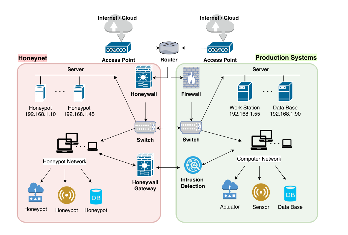
Based on the network topology, we introduce the continuous-time infinite-horizon discounted SMDPs, which can be summarized by the tuple . We illustrate each element of the tuple through a -state example in Fig. 9.
Each node in Fig. 9 represents a state . At time , the attacker is either at one of the honeypot node denoted by state , at the normal zone , or at a virtual absorbing state once attackers are ejected or terminate on their own. At each state , the defender can choose an action . For example, at honeypot nodes, the defender can conduct action to eject the attacker, action to purely record the attacker’s activities, low-interactive action , or high-interactive action , i.e., . The high-interactive action is costly to implement yet can both increases the probability of a longer sojourn time at honeypot , and reduces the probability of attackers penetrating the normal system from if connected. If the attacker resides in the normal zone either from the beginning or later through the pivot honeypots, the defender can choose either action to eject the attacker immediately, or action to attract the attacker to the honeynet by generating more deceptive inbound and outbound traffics in the honeynet, i.e., .
t]
Based on the current state and the defender’s action , the attacker transits to state with probability and the sojourn time at state is a continuous random variable with probability density . Once the attacker arrives at a new honeypot , the defender dynamically applies an interaction action at honeypot from and keeps interacting with the attacker until she transits to the next honeypot. If the defender changes the action before the transition, the attacker may be able to detect the change and become aware of the honeypot. Since the decision is made at the time of transition, we can transform the above continuous time model on horizon into a discrete decision model at decision epoch . The time of the attacker’s transition is denoted by a random variable , the landing state is denoted as , and the adopted action after arriving at is denoted as .
The defender gains an investigation reward by engaging and analyzing the attacker in the honeypot. To simplify the notation, we segment the investigation reward during time into ones at discrete decision epochs . When amount of time elapses at stage , the defender’s investigation reward , at time of stage , is the sum of two parts. The first part is the immediate cost of applying engagement action at state and the second part is the reward rate of threat information acquisition minus the cost rate of persistently generating deceptive traffics. Due to the randomness of the attacker’s behavior, the information acquisition can also be random, thus the actual reward rate is perturbed by an additive zero-mean noise . As the defender spends longer time interacting with attackers, investigating their behaviors and acquires better understandings of their targets and TTPs, less new information can be extracted. In addition, the same intelligence becomes less valuable as time elapses due to the timeliness. Thus, we use a discounted factor of to penalize the decreasing value of the investigation reward as time elapses.
The defender aims at a policy which maps state to action to maximize the long-term expected utility starting from state , i.e.,
| (17) |
At each decision epoch, the value function can be represented by dynamic programming, i.e.,
| (18) |
We assume a constant reward rate for simplicity. Then, (18) can be transformed into an equivalent MDP form, i.e., ,
| (19) |
where is the Laplace transform of the sojourn probability density and the equivalent reward is assumed to be bounded by a constant .
Definition 3
There exists constants and such that
| (20) |
∎
The right-hand side of (18) is a contraction mapping under the regulation condition in Definition 3. Then, we can find the unique optimal policy by value iteration, policy iteration or linear programming. Fig. 9 illustrates the optimal policy and the state value by the color and the size of the node, respectively. In the example scenario, the honeypot of database and sensors are the main and secondary targets of the attacker, respectively. Thus, defenders can obtain a higher investigation reward when they manage to engage the attacker in these two honeypot nodes with a larger probability and for a longer time. However, instead of naively adopting high interactive actions, a savvy defender also balances the high implantation cost of . Our quantitative results indicate that the high interactive action should only be applied at to be cost-effective. On the other hand, although the bridge nodes which connect to the normal zone do not contain higher investigation rewards than other nodes, the defender still takes action at these nodes. The goal is to either increase the probability of attracting attackers away from the normal zone or reduce the probability of attackers penetrating the normal zone from these bridge nodes.
4.2 Reinforcement Learning of SMDP
The absent knowledge of the attacker’s characteristics results in environmental uncertainty of the investigation reward, the attacker’s transition probability, and the sojourn distribution. We use -learning algorithm to obtain the optimal engagement policy based on the actual experience of the honeynet interactions, i.e., ,
| (21) |
where is the learning rate, are the observed states at stage and , is the observed investigation rewards, and is the observed sojourn time at state . When the learning rate satisfies the condition of convergency in Definition 2, i.e., , and all state-action pairs are explored infinitely, , in (21) converges to value with probability .
At each decision epoch , the action is chosen according to the -greedy policy, i.e., the defender chooses the optimal action with a probability , and a random action with a probability . Note that the exploration rate should not be too small to guarantee sufficient samples of all state-action pairs. The -learning algorithm under a pure exploration policy still converges yet at a slower rate.
t]
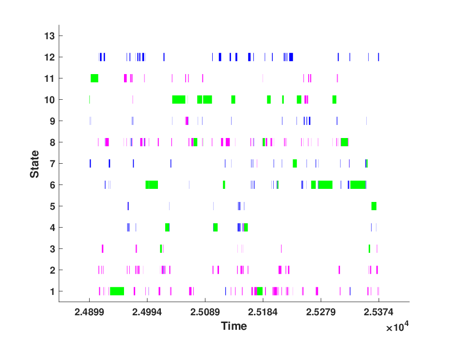
In our scenario, the defender knows the reward of ejection action and , thus does not need to explore action to learn it. We plot one learning trajectory of the state transition and sojourn time under the -greedy exploration policy in Fig. 10, where the chosen actions are denoted in red, blue, purple, and green, respectively. If the ejection reward is unknown, the defender should be restrictive in exploring which terminates the learning process. Otherwise, the defender may need to engage with a group of attackers who share similar behaviors to obtain sufficient samples to learn the optimal engagement policy.
In particular, we choose , to guarantee the asymptotic convergence, where is a constant parameter and is the number of visits to state-action pair up to stage . We need to choose a proper value of to guarantee a good numerical performance of convergence in finite steps as shown in Fig. 11(a). We shift the green and blue lines vertically to avoid the overlap with the red line and represent the corresponding theoretical values in dotted black lines. If is too small as shown in the red line, the learning rate decreases so fast that new observed samples hardly update the -value and the defender may need a long time to learn the right value. However, if is too large as shown in the green line, the learning rate decreases so slow that new samples contribute significantly to the current -value. It causes a large variation and a slower convergence rate of .
We show the convergence of the policy and value under , in the video demo (See URL: https://bit.ly/2QUz3Ok). In the video, the color of each node distinguishes the defender’s action at state and the size of the node is proportional to at stage . To show the convergence, we decrease the value of gradually to after steps. Since the convergence trajectory is stochastic, we run the simulation for times and plot the mean and the variance of of state under the optimal policy in Fig. 11. The mean in red converges to the theoretical value in about steps and the variance in blue reduces dramatically as step increases.
5 Conclusion and Discussion
This chapter has introduced three defense schemes, i.e., defensive deception to detect and counter adversarial deception, feedback-driven Moving Target Defense (MTD) to increase the attacker’s probing and reconnaissance costs, and adaptive honeypot engagement to gather fundamental threat information. These schemes satisfy the Principle of 3A Defense as they actively protect the system prior to the attack damages, provide strategic defenses autonomously, and apply learning to adapt to uncertainty and changes. These schemes possess three progressive levels of information restrictions, which lead to different strategic learning schemes to estimate the parameter, the payoff, and the environment. All these learning schemes, however, have a feedback loop to sense samples, estimate the unknowns, and take actions according to the estimate. Our work lays a solid foundation for strategic learning in active, adaptive, autonomous defenses under incomplete information and leads to the following challenges and future directions.
First, multi-agent learning in non-cooperative environments is challenging due to the coupling and interaction between these heterogeneous agents. The learning results depend on all involving agents yet other players’ behaviors, levels of rationality, and learning schemes are not controllable and may change abruptly. Moreover, as attackers become aware of the active defense techniques and the learning scheme under incomplete information, the savvy attacker can attempt to interrupt the learning process. For example, attackers may sacrifice their immediate rewards and take incomprehensible actions instead so that the defender learns incorrect attack characteristics. The above challenges motivate robust learning methods under non-cooperative and even adversarial environments.
Second, since the learning process is based on samples from real interactions, the defender needs to concern the system safety and security during the learning period, while in the same time, attempts to achieve more accurate learning results of the attack’s characteristics. Moreover, since the learning under non-cooperative and adversarial environments may terminate unpredictably at any time, the asymptotic convergence would not be critical for security. The defender needs to care more about the time efficiency of the learning, i.e., how to achieve a sufficiently good estimate in a finite number of steps.
Third, instead of learning from scratch, the defender can attempt to reuse the past experience with attackers of similar behaviors to expedite the learning process, which motivates the investigation of transfer learning in reinforcement learning taylor2009transfer. Some side-channel information may also contribute to the learning to allow agents to learn faster.
References
- (1) “Verizon 2019 data breach investigations report,” 2019.
- (2) D. Shackleford, “Combatting cyber risks in the supply chain,” SANS. org, 2015.
- (3) L. Huang and Q. Zhu, “Adaptive strategic cyber defense for advanced persistent threats in critical infrastructure networks,” ACM SIGMETRICS Performance Evaluation Review, vol. 46, no. 2, pp. 52–56, 2019.
- (4) ——, “Analysis and computation of adaptive defense strategies against advanced persistent threats for cyber-physical systems,” in International Conference on Decision and Game Theory for Security. Springer, 2018, pp. 205–226.
- (5) L. Huang and Q. Zhu, “A Dynamic Games Approach to Proactive Defense Strategies against Advanced Persistent Threats in Cyber-Physical Systems,” arXiv e-prints, p. arXiv:1906.09687, Jun 2019.
- (6) Q. Zhu and T. Başar, “Game-theoretic approach to feedback-driven multi-stage moving target defense,” in International Conference on Decision and Game Theory for Security. Springer, 2013, pp. 246–263.
- (7) L. Huang and Q. Zhu, “Adaptive Honeypot Engagement through Reinforcement Learning of Semi-Markov Decision Processes,” arXiv e-prints, p. arXiv:1906.12182, Jun 2019.
- (8) J. Pawlick, E. Colbert, and Q. Zhu, “A game-theoretic taxonomy and survey of defensive deception for cybersecurity and privacy,” arXiv preprint arXiv:1712.05441, 2017.
- (9) F. J. Stech, K. E. Heckman, and B. E. Strom, “Integrating cyber-d&d into adversary modeling for active cyber defense,” in Cyber deception. Springer, 2016, pp. 1–22.
- (10) K. E. Heckman, M. J. Walsh, F. J. Stech, T. A. O’boyle, S. R. DiCato, and A. F. Herber, “Active cyber defense with denial and deception: A cyber-wargame experiment,” computers & security, vol. 37, pp. 72–77, 2013.
- (11) J. Gómez-Hernández, L. Álvarez-González, and P. García-Teodoro, “R-locker: Thwarting ransomware action through a honeyfile-based approach,” Computers & Security, vol. 73, pp. 389–398, 2018.
- (12) N. Virvilis, B. Vanautgaerden, and O. S. Serrano, “Changing the game: The art of deceiving sophisticated attackers,” in 2014 6th International Conference On Cyber Conflict (CyCon 2014). IEEE, 2014, pp. 87–97.
- (13) J. Pawlick, E. Colbert, and Q. Zhu, “Modeling and analysis of leaky deception using signaling games with evidence,” IEEE Transactions on Information Forensics and Security, 2018.
- (14) S. Jajodia, A. K. Ghosh, V. Swarup, C. Wang, and X. S. Wang, Moving target defense: creating asymmetric uncertainty for cyber threats. Springer Science & Business Media, 2011, vol. 54.
- (15) G. S. Kc, A. D. Keromytis, and V. Prevelakis, “Countering code-injection attacks with instruction-set randomization,” in Proceedings of the 10th ACM conference on Computer and communications security. ACM, 2003, pp. 272–280.
- (16) A. Clark, Q. Zhu, R. Poovendran, and T. Başar, “Deceptive routing in relay networks,” in International Conference on Decision and Game Theory for Security. Springer, 2012, pp. 171–185.
- (17) H. Maleki, S. Valizadeh, W. Koch, A. Bestavros, and M. van Dijk, “Markov modeling of moving target defense games,” in Proceedings of the 2016 ACM Workshop on Moving Target Defense. ACM, 2016, pp. 81–92.
- (18) C. R. Hecker, “A methodology for intelligent honeypot deployment and active engagement of attackers,” Ph.D. dissertation, 2012.
- (19) Q. D. La, T. Q. Quek, J. Lee, S. Jin, and H. Zhu, “Deceptive attack and defense game in honeypot-enabled networks for the internet of things,” IEEE Internet of Things Journal, vol. 3, no. 6, pp. 1025–1035, 2016.
- (20) J. Pawlick, T. T. H. Nguyen, and Q. Zhu, “Optimal timing in dynamic and robust attacker engagement during advanced persistent threats,” CoRR, vol. abs/1707.08031, 2017. [Online]. Available: http://arxiv.org/abs/1707.08031
- (21) J. Pawlick and Q. Zhu, “A Stackelberg game perspective on the conflict between machine learning and data obfuscation,” in Information Forensics and Security (WIFS), 2016 IEEE International Workshop on. IEEE, 2016, pp. 1–6. [Online]. Available: http://ieeexplore.ieee.org/abstract/document/7823893/
- (22) Q. Zhu, A. Clark, R. Poovendran, and T. Basar, “Deployment and exploitation of deceptive honeybots in social networks,” in Decision and Control (CDC), 2013 IEEE 52nd Annual Conference on. IEEE, 2013, pp. 212–219.
- (23) Q. Zhu, H. Tembine, and T. Basar, “Hybrid learning in stochastic games and its applications in network security,” Reinforcement Learning and Approximate Dynamic Programming for Feedback Control, pp. 305–329, 2013.
- (24) Q. Zhu, Z. Yuan, J. B. Song, Z. Han, and T. Başar, “Interference aware routing game for cognitive radio multi-hop networks,” Selected Areas in Communications, IEEE Journal on, vol. 30, no. 10, pp. 2006–2015, 2012.
- (25) Q. Zhu, L. Bushnell, and T. Basar, “Game-theoretic analysis of node capture and cloning attack with multiple attackers in wireless sensor networks,” in Decision and Control (CDC), 2012 IEEE 51st Annual Conference on. IEEE, 2012, pp. 3404–3411.
- (26) Q. Zhu, A. Clark, R. Poovendran, and T. Başar, “Deceptive routing games,” in Decision and Control (CDC), 2012 IEEE 51st Annual Conference on. IEEE, 2012, pp. 2704–2711.
- (27) Q. Zhu, H. Li, Z. Han, and T. Basar, “A stochastic game model for jamming in multi-channel cognitive radio systems.” in ICC, 2010, pp. 1–6.
- (28) Z. Xu and Q. Zhu, “Secure and practical output feedback control for cloud-enabled cyber-physical systems,” in Communications and Network Security (CNS), 2017 IEEE Conference on. IEEE, 2017, pp. 416–420.
- (29) ——, “A Game-Theoretic Approach to Secure Control of Communication-Based Train Control Systems Under Jamming Attacks,” in Proceedings of the 1st International Workshop on Safe Control of Connected and Autonomous Vehicles. ACM, 2017, pp. 27–34. [Online]. Available: http://dl.acm.org/citation.cfm?id=3055381
- (30) ——, “Cross-layer secure cyber-physical control system design for networked 3d printers,” in American Control Conference (ACC), 2016. IEEE, 2016, pp. 1191–1196. [Online]. Available: http://ieeexplore.ieee.org/abstract/document/7525079/
- (31) M. J. Farooq and Q. Zhu, “Modeling, analysis, and mitigation of dynamic botnet formation in wireless iot networks,” IEEE Transactions on Information Forensics and Security, 2019.
- (32) Z. Xu and Q. Zhu, “A cyber-physical game framework for secure and resilient multi-agent autonomous systems,” in Decision and Control (CDC), 2015 IEEE 54th Annual Conference on. IEEE, 2015, pp. 5156–5161.
- (33) L. Huang, J. Chen, and Q. Zhu, “A large-scale markov game approach to dynamic protection of interdependent infrastructure networks,” in International Conference on Decision and Game Theory for Security. Springer, 2017, pp. 357–376.
- (34) J. Chen, C. Touati, and Q. Zhu, “A dynamic game analysis and design of infrastructure network protection and recovery,” ACM SIGMETRICS Performance Evaluation Review, vol. 45, no. 2, p. 128, 2017.
- (35) F. Miao, Q. Zhu, M. Pajic, and G. J. Pappas, “A hybrid stochastic game for secure control of cyber-physical systems,” Automatica, vol. 93, pp. 55–63, 2018.
- (36) Y. Yuan, Q. Zhu, F. Sun, Q. Wang, and T. Basar, “Resilient control of cyber-physical systems against denial-of-service attacks,” in Resilient Control Systems (ISRCS), 2013 6th International Symposium on. IEEE, 2013, pp. 54–59.
- (37) S. Rass and Q. Zhu, “GADAPT: A Sequential Game-Theoretic Framework for Designing Defense-in-Depth Strategies Against Advanced Persistent Threats,” in Decision and Game Theory for Security, ser. Lecture Notes in Computer Science, Q. Zhu, T. Alpcan, E. Panaousis, M. Tambe, and W. Casey, Eds. Cham: Springer International Publishing, 2016, vol. 9996, pp. 314–326.
- (38) Q. Zhu, Z. Yuan, J. B. Song, Z. Han, and T. Basar, “Dynamic interference minimization routing game for on-demand cognitive pilot channel,” in Global Telecommunications Conference (GLOBECOM 2010), 2010 IEEE. IEEE, 2010, pp. 1–6.
- (39) T. Zhang and Q. Zhu, “Strategic defense against deceptive civilian gps spoofing of unmanned aerial vehicles,” in International Conference on Decision and Game Theory for Security. Springer, 2017, pp. 213–233.
- (40) L. Huang and Q. Zhu, “Analysis and computation of adaptive defense strategies against advanced persistent threats for cyber-physical systems,” in International Conference on Decision and Game Theory for Security, 2018.
- (41) ——, “Adaptive strategic cyber defense for advanced persistent threats in critical infrastructure networks,” in ACM SIGMETRICS Performance Evaluation Review, 2018.
- (42) J. Pawlick, S. Farhang, and Q. Zhu, “Flip the cloud: Cyber-physical signaling games in the presence of advanced persistent threats,” in Decision and Game Theory for Security. Springer, 2015, pp. 289–308.
- (43) S. Farhang, M. H. Manshaei, M. N. Esfahani, and Q. Zhu, “A dynamic bayesian security game framework for strategic defense mechanism design,” in Decision and Game Theory for Security. Springer, 2014, pp. 319–328.
- (44) Q. Zhu and T. Başar, “Dynamic policy-based ids configuration,” in Decision and Control, 2009 held jointly with the 2009 28th Chinese Control Conference. CDC/CCC 2009. Proceedings of the 48th IEEE Conference on. IEEE, 2009, pp. 8600–8605.
- (45) Q. Zhu, H. Tembine, and T. Basar, “Network security configurations: A nonzero-sum stochastic game approach,” in American Control Conference (ACC), 2010. IEEE, 2010, pp. 1059–1064.
- (46) Q. Zhu, H. Tembine, and T. Başar, “Heterogeneous learning in zero-sum stochastic games with incomplete information,” in 49th IEEE conference on decision and control (CDC). IEEE, 2010, pp. 219–224.
- (47) J. Chen and Q. Zhu, “Security as a Service for Cloud-Enabled Internet of Controlled Things under Advanced Persistent Threats: A Contract Design Approach,” IEEE Transactions on Information Forensics and Security, 2017. [Online]. Available: http://ieeexplore.ieee.org/abstract/document/7954676/
- (48) R. Zhang, Q. Zhu, and Y. Hayel, “A Bi-Level Game Approach to Attack-Aware Cyber Insurance of Computer Networks,” IEEE Journal on Selected Areas in Communications, vol. 35, no. 3, pp. 779–794, 2017. [Online]. Available: http://ieeexplore.ieee.org/abstract/document/7859343/
- (49) R. Zhang and Q. Zhu, “Attack-aware cyber insurance of interdependent computer networks,” 2016.
- (50) W. A. Casey, Q. Zhu, J. A. Morales, and B. Mishra, “Compliance control: Managed vulnerability surface in social-technological systems via signaling games,” in Proceedings of the 7th ACM CCS International Workshop on Managing Insider Security Threats. ACM, 2015, pp. 53–62.
- (51) Y. Hayel and Q. Zhu, “Attack-aware cyber insurance for risk sharing in computer networks,” in Decision and Game Theory for Security. Springer, 2015, pp. 22–34.
- (52) ——, “Epidemic protection over heterogeneous networks using evolutionary poisson games,” IEEE Transactions on Information Forensics and Security, vol. 12, no. 8, pp. 1786–1800, 2017.
- (53) Q. Zhu, C. Fung, R. Boutaba, and T. Başar, “Guidex: A game-theoretic incentive-based mechanism for intrusion detection networks,” Selected Areas in Communications, IEEE Journal on, vol. 30, no. 11, pp. 2220–2230, 2012.
- (54) Q. Zhu, C. A. Gunter, and T. Basar, “Tragedy of anticommons in digital right management of medical records.” in HealthSec, 2012.
- (55) Q. Zhu, C. Fung, R. Boutaba, and T. Başar, “A game-theoretical approach to incentive design in collaborative intrusion detection networks,” in Game Theory for Networks, 2009. GameNets’ 09. International Conference on. IEEE, 2009, pp. 384–392.
- (56) T. E. Carroll and D. Grosu, “A game theoretic investigation of deception in network security,” Security and Commun. Nets., vol. 4, no. 10, pp. 1162–1172, 2011.
- (57) J. Pawlick and Q. Zhu, “A Stackelberg game perspective on the conflict between machine learning and data obfuscation,” IEEE Intl. Workshop on Inform. Forensics and Security, 2016.
- (58) T. Zhang and Q. Zhu, “Dynamic differential privacy for ADMM-based distributed classification learning,” IEEE Transactions on Information Forensics and Security, vol. 12, no. 1, pp. 172–187, 2017. [Online]. Available: http://ieeexplore.ieee.org/abstract/document/7563366/
- (59) S. Farhang, Y. Hayel, and Q. Zhu, “Phy-layer location privacy-preserving access point selection mechanism in next-generation wireless networks,” in Communications and Network Security (CNS), 2015 IEEE Conference on. IEEE, 2015, pp. 263–271.
- (60) T. Zhang and Q. Zhu, “Distributed privacy-preserving collaborative intrusion detection systems for vanets,” IEEE Transactions on Signal and Information Processing over Networks, vol. 4, no. 1, pp. 148–161, 2018.
- (61) N. Zhang, W. Yu, X. Fu, and S. K. Das, “gPath: A game-theoretic path selection algorithm to protect tor’s anonymity,” in Decision and Game Theory for Security. Springer, 2010, pp. 58–71.
- (62) A. Garnaev, M. Baykal-Gursoy, and H. V. Poor, “Security games with unknown adversarial strategies,” IEEE transactions on cybernetics, vol. 46, no. 10, pp. 2291–2299, 2015.
- (63) Q. Zhu, H. Tembine, and T. Başar, “Distributed strategic learning with application to network security,” in Proceedings of the 2011 American Control Conference. IEEE, 2011, pp. 4057–4062.
- (64) A. Servin and D. Kudenko, “Multi-agent reinforcement learning for intrusion detection: A case study and evaluation,” in German Conference on Multiagent System Technologies. Springer, 2008, pp. 159–170.
- (65) P. M. Djurić and Y. Wang, “Distributed bayesian learning in multiagent systems: Improving our understanding of its capabilities and limitations,” IEEE Signal Processing Magazine, vol. 29, no. 2, pp. 65–76, 2012.
- (66) G. Chalkiadakis and C. Boutilier, “Coordination in multiagent reinforcement learning: a bayesian approach,” in Proceedings of the second international joint conference on Autonomous agents and multiagent systems. ACM, 2003, pp. 709–716.
- (67) Z. Chen and D. Marculescu, “Distributed reinforcement learning for power limited many-core system performance optimization,” in Proceedings of the 2015 Design, Automation & Test in Europe Conference & Exhibition. EDA Consortium, 2015, pp. 1521–1526.
- (68) J. C. Harsanyi, “Games with incomplete information played by “bayesian” players, i–iii part i. the basic model,” Management science, vol. 14, no. 3, pp. 159–182, 1967.
- (69) M. E. Taylor and P. Stone, “Transfer learning for reinforcement learning domains: A survey,” Journal of Machine Learning Research, vol. 10, no. Jul, pp. 1633–1685, 2009.