Field theory approach to the quantum transport in Weyl semimetals

The Weyl points in a topological semimetal appear always in pairs with opposite chirality nielsen1981. For this reason, a minimal model describing a realistic Weyl semimetal must include two band-touching points and break time-reversal invariance, as in the case of layered intermetallic materials with a trigonal crystal structure soh2019. Our starting point is therefore a toy model of fermions with a suitable pseudospin-1/2 degree of freedom, that can represent orbital, sublattice or spin degrees of freedom. The fermions move on a cubic lattice with a dynamics dictated by the Hamiltonian $H_{\rm lat}=\sum_{\bf p}c^{\dagger}_{\bf p}H_{\rm lat}({\bf p})c_{\bf p}$, where $c$ and $c^{\dagger}$ are two-component spinors and:

$$H_{\rm lat}({\bf p})=\tilde{v}\left(\cos p_{0}-\cos p_{x}\right)\sigma_{x}+\\ v\left(2-\cos p_{y}-\cos p_{z}\right)\sigma_{x}+v\sin p_{y}\sigma_{y}+v\sin p_{z}\sigma_{z}\,.$$

(II.1)

In this equation, the Pauli matrices $\sigma_{i}$ act on the pseudospin, and hereafter we adopt units such that the lattice spacing is unity.

This minimal model yang2011; okugawa2014; lopez2018 displays two Weyl points in $\left(\pm p_{0},0,0\right)$ at zero energy, and we choose $\tilde{v}=v/\sin p_{0}$ in order to obtain an isotropic energy dispersion around both. For $\tilde{v}\cos p_{0}\neq 0$, the Hamiltonian (II.1) corresponds to a stack of 2-dimensional topological insulators laying on the $yz$ planes and coupled by the tunneling term along the $\hat{x}$ direction. In particular, in the two-dimensional $yz$ limit described by $\cos{p_{x}}=0$, we obtain a topological insulator with chiral gapless edge modes for $\tilde{v}\cos{p_{0}}<0$. When introducing the coupling in the $\hat{x}$ direction, these gapless modes evolve into Fermi arcs localized on the surfaces $xy$ and $xz$.

The Hamiltonian (II.1) is invariant under space-inversion symmetry,

$$H_{\rm lat}(-{\bf p})=U\,H_{\rm lat}({\bf p})\,U^{-1},\quad\text{with }\;U=\sigma_{x}\,,$$

(II.2)

in such a way that the two Weyl points appear at the same energy. Concerning its boundaries, we neglect band-bending potentials at the surface; as a result, the Fermi arcs in this system do not display a spiraling dispersion, differently from the setups analyzed in Ref. andreev15 (see also Ref. lepori16 for the effect of trapping potentials).

To analytically study the behavior of the surface states, for small values of $p_{0}$, we approximate the low-energy behavior of (II.1) with the Hamiltonian

$$H({\bf p})=\frac{{v}}{2p_{0}}\left(p_{x}^{2}-p_{0}^{2}\right)\sigma_{x}+vp_{y}\sigma_{y}+vp_{z}\sigma_{z}\,,$$

(II.3)

leading to the differential operator

$$H(-i{\bf\nabla})=-\frac{{v}}{2p_{0}}\left(\partial_{x}^{2}+p_{0}^{2}\right)\sigma_{x}-vi\partial_{y}\sigma_{y}-vi\partial_{z}\sigma_{z}\,.$$

(II.4)

Let us assume that the Weyl semimetal is located in the half-space ${\mathbb{R}}^{3}_{+}$ with $z>0$. Then (II.4) defines a symmetric operator on a suitable set ${\cal D}({\mathbb{R}}^{3}_{+})$ of smooth functions, which is dense in the set of square integrable functions on ${\mathbb{R}}^{3}_{+}$. The general theory (see e.g. Ref. RS) of such operators implies in our case that $H(-i{\bf\nabla})$ has self-adjoint extensions, which involve one real parameter. The nature of this parameter can be deduced from the condition

$$\langle\psi H(-i{\bf\nabla})|\varphi\rangle-\langle\psi|H(-i{\bf\nabla})\varphi\rangle=0\,,$$

(II.5)

imposed for each pair of wave functions $\psi$ and $\varphi$ in the domain ${\cal D}({\mathbb{R}}^{3}_{+})$. The previous relation is equivalent to the surface condition

$$\varphi^{\dagger}(\bm{r})\sigma_{z}\psi(\bm{r})\,\bigr|_{z=0}=0\,,$$

(II.6)

where ^† stands for Hermitian conjugation. Analogously to the 2D case of graphene mccann2004; akhmerov2008, Eq. (II.6) corresponds to the physical requirement of vanishing of the probability current flowing across the surface $z=0$. It is satisfied by the (maximal) set of wave functions with an arbitrary and translationally invariant polarization of the pseudospin parallel to the surface in all its points, namely

$$\left(\sigma_{x}\cos\gamma+\sigma_{y}\sin\gamma\right)\psi(\bm{r})\,\bigr|_{z=0}=\psi(\bm{r})\,\bigr|_{z=0}\,.$$

(II.7)

The angle $0\leq\gamma<2\pi$ parametrizes all the self-adjoint extensions $H_{\gamma}$ of the Hamiltonian (II.3) and specifies the pseudospin polarization in the plane $xy$ of all the wavefunctions on the surface $z=0$. In the physical context the parameter $\gamma$ is expected to depend in general on the electric/magnetic properties of the Weyl material and the termination of its lattice that defines the surface, as experimentally verified in Refs. souma2016; morali2019.

Once $\gamma\in[0,2\pi)$ is fixed, the spectral properties of $H_{\gamma}$ are uniquely determined and concisely described in Appendix A. Summarizing, the eigenfunctions

$$\{\zeta_{\rm s}^{\pm}({\bf r},p),\,\zeta_{\rm b}^{\pm}({\bf r,p})\}$$

(II.8)

are of two different types, called in what follows surface and bulk states. The surface eigenstates $\zeta_{\rm s}^{\pm}({\bf r},p)$, given by (A.1), depend only on the two momenta $p=(p_{x},p_{y})$ parallel to the $z$-plane and decay exponentially along the $z$-axis. The bulk eigenstates $\zeta_{\rm b}^{\pm}({\bf r,p})$, given by (A.2,A.3), depend instead on all the three momenta ${\bf p}=(p_{x},p_{y},p_{z})$ and oscillate along the $z$-axis. The associated eigenvalues

$$\{\varepsilon_{\rm s}(p),\,\pm\varepsilon_{\rm b}({\bf p})\}$$

(II.9)

are expressed in terms of the combinations

$$g(p_{x})=\frac{p_{x}^{2}-p_{0}^{2}}{2p_{0}}\,,\quad\tilde{p}_{z}(p)=p_{y}\cos\gamma-g(p_{x})\sin\gamma\,.$$

(II.10)

In particular, the surface states $\zeta_{\rm s}^{\pm}({\bf r},p)$ correspond to the domains in momentum space with positive and negative energies $\varepsilon_{\rm s}(p)$ respectively. These surface eigenvalues of the Hamiltonian are defined by:

$$\varepsilon_{\rm s}(p)=v\left[g(p_{x})\cos\gamma+p_{y}\sin\gamma\right]\,,\quad\tilde{p}_{z}(p)>0\,.$$

(II.11)

The bulk energies result instead:

$$\varepsilon_{\rm b}({\bf p})=v\sqrt{g(p_{x})^{2}+p_{y}^{2}+p_{z}^{2}}\,,\quad p_{z}{\geq}0\,.$$

(II.12)

The eigenvectors (II.8) form a complete orthogonal basis, which together with (II.11,II.12), defines uniquelyRS the self-adjoint extension $H_{\gamma}$.

The $\gamma$-dependence of the energy spectrum is a first indication that the physics of our system depends on the boundary conditions. It is instructive to consider in this respect the zero-energy eigenstates. There are four bulk states with this property, corresponding to the spin-degenerate states at the momenta $(p_{x}=\pm p_{0},\,p_{y}=0,\,p_{z}=0)$. In addition, there is the family of surface states with vanishing energy

$$p_{y}=-g(p_{x})\cot\gamma\,,\qquad\tilde{p}_{z}(p)>0\,.$$

(II.13)

associated with the dispersion relation (II.11). The set of all these zero-energy eigenstates form the open Fermi arc on the surface Brillouin zone. In fact, equation (II.11) defines the shape of the arc which depends explicitly on the angle $\gamma$, which gives its orientation at the limiting points $(p_{x}=\pm p_{0},\,p_{y}=0,\,p_{z}=0)$ (measured from the upper vertical direction clockwise and counterclockwise respectively, see Fig. 1). In particular, for $p_{x}=p_{0}$, the Fermi arc is always oriented orthogonally to the pseudospin polarization given by the boundary conditions (II.7). In the range $0<\gamma<\pi$, the length $L_{\rm FA}(\gamma)$ of the Fermi arcs following from (II.13) is

$$L_{\rm FA}(\gamma)=p_{0}\left\{\frac{1}{\sin\gamma}+(\tan\gamma)\log\left[\frac{1+\cos\gamma}{\sin\gamma}\right]\right\}\,.$$

(II.14)

We find Eq. (II.14) instructive because it relates the angle $\gamma$, which has an abstract mathematical origin, with the length of the Fermi arc $L_{\rm FA}$ and with $p_{0}$, which are experimentally measurable quantities in ARPES measurements xu2015; xu2015_3; souma2016; morali2019.

The value $\gamma=\pi/2$ describes a straight Fermi arc connecting the projections of the Weyl points. In fact, at this point the function (II.14) reaches its minimum $L_{\rm FA}(\pi/2)=2p_{0}$. For $\gamma=0$ and $\gamma=\pi$ the orientation of the Fermi arc becomes orthogonal to the line connecting the Weyl points: in this case and, more in general, for $\pi\leq\gamma\leq 2\pi$, our choice of the function $g$ returns indeed two distinct and unbounded Fermi arcs. In tight-binding models of real materials, the two branches are always connected with each other, but our second-order approximation of the lattice Hamiltonian (II.1) describes only their behavior in proximity of the Weyl point projections and fails in depicting the global behavior of the Fermi arc across the Brillouin zone. The regime $\pi\leq\gamma\leq 2\pi$ may indeed correspond to systems and surfaces in which a Fermi arc connects Weyl points in adjacent Brillouin zones (see, for example, the recent experimental results in Ref. morali2019).

The above approach is very general and applies to other Hamiltonians in spaces with boundary as well. We stress in this respect that once the Hamiltonian $H$ is fixed, there is no further freedom for choosing neither the boundary condition nor the number of parameters, describing its self-adjoint extensions. In fact, the boundary condition is uniquely determined by requiring the Hermiticity (II.5) of $H$, whereas the number of parameters is fixed by the indices $n_{\pm}$ associated to $H$ (see e.g. Ref. RS for details). If $n_{-}=n_{+}\equiv n$ according to the Von Neumann theoremRS $H$ admits a $n^{2}$-parameter family self-adjoint extensions. According to (II.7) a single angle $\gamma$ determines all self-adjoint extensions of the Hamiltonian (II.4), which implies that in our case $n=1$. This is related to our choice of a minimal 2-component model Hamiltonian for the description of the Weyl semimetal. We observe, however, that in the literature Dirac Hamiltonians involving 4-component spinors are often adopted to describe this kind of systems (see, for example, faraei18; faraei2019 and the analogous case for graphene akhmerov2008). In that case the self-adjoint extensions depend on a larger set of parameters. For the sake of simplicity we base our analysis on the model in Eq. (II.3), which allows us to capture all the main physical features of the surface transport of Weyl semimetals, without resorting to larger spinors.

Summarizing, the Hamiltonian $H_{\gamma}$ on the half space ${\mathbb{R}}^{3}_{+}$ has quite remarkable spectral properties, which represent the core of the quantum field description developed below. In particular, the main physical properties of the surface states can be derived from the Hamiltonian (II.3) for boundary conditions with $0<\gamma<\pi$. In the remainder of the paper, this regime will be assumed.

The strategy is well known and aims at the construction of a quantum field

$$\Psi(t,{\bf r})=\Psi_{\rm s}(t,{\bf r})+\Psi_{\rm b}(t,{\bf r})\,,$$

(II.15)

where $\Psi_{\rm s}$ and $\Psi_{\rm b}$ collect the bulk and surface contributions. The fundamental requirements are that the time evolution of $\Psi$ is generated by $H_{\gamma}$ and that $\Psi$ satisfies the canonical equal-time anti-commutation relations. In order to write the solution in explicit form we adopt for later convenience a Dirac type formulation and introduce the following notation: we label by $a_{\rm s}$ and $a_{\rm s}^{\dagger}$ the annihilation and creation operators for surface quasiparticles with $\varepsilon_{\rm s}>0$, and by $b_{\rm s}$ and $b_{\rm s}^{\dagger}$ the annihilation and creation operators for surface quasiholes, such that:

	$\displaystyle a_{\rm s}(p)$	$\displaystyle=c_{\rm s}(p)\Theta\left[\varepsilon_{\rm s}(p)\right]\,,$		(II.16)
	$\displaystyle b_{\rm s}(-p)$	$\displaystyle=c_{\rm s}^{\dagger}(p)\Theta\left[-\varepsilon_{\rm s}(p)\right]\,,$		(II.17)

where the operators $c_{\rm s}(p)$ are annihilation operators of the electrons on the surface and $\Theta$ is the Heaviside step function. Analogously, we set in the bulk

	$\displaystyle a_{\rm b}({\bf p})$	$\displaystyle=c_{\rm b}({\bf p})\Theta\left[\varepsilon_{\rm b}({\bf p})\right]\,,$		(II.18)
	$\displaystyle b_{\rm b}(-{\bf p})$	$\displaystyle=c_{\rm b}^{\dagger}({\bf p})\Theta\left[-\varepsilon_{\rm b}({\bf p})\right]\,,$		(II.19)

where $c_{\rm b}({\bf p})$ are the annihilation operators of the electrons in the bulk. With these conventions $\Psi_{\rm s}$ and $\Psi_{\rm b}$ take the form

	$\displaystyle\Psi_{\rm s}(t,\bm{r})$	$\displaystyle=\int\displaylimits\frac{d^{2}p}{(2\pi)^{2}}\left[a_{\rm s}(p)\zeta_{\rm s}^{(+)}({\bm{r}},p){\rm e}^{-it\left|\varepsilon_{\rm s}(p)\right|}+b_{\rm s}^{\dagger}(-p)\zeta_{\rm s}^{(-)}({\bm{r}},p){\rm e}^{it\left|\varepsilon_{\rm s}(p)\right|}\right]\,,$		(II.20)
	$\displaystyle\Psi_{\rm b}(t,\bm{r})$	$\displaystyle=\int\displaylimits\frac{d^{3}p}{(2\pi)^{3}}\left[a_{\rm b}(\bm{p})\zeta_{\rm b}^{(+)}(\bm{r,p}){\rm e}^{-it\left|\varepsilon_{\rm b}(\bm{p})\right|}+b_{\rm b}^{\dagger}(-\bm{p})\zeta_{\rm b}^{(-)}(\bm{r,p}){\rm e}^{it\left|\varepsilon_{\rm b}(\bm{p})\right|}\right]\,,$		(II.21)

in terms of the complete system (II.8) of eigenfunctions of $H_{\gamma}$ and the creation and annihilation operators (II.16-II.19), satisfying the canonical anti-commutation relations. We observe that the surface and the bulk components (II.20,II.21) obey separately the equation of motion. This is not he case for the equal-time canonical anti-commutation relations, which follow from the completeness of the energy eigenstates and hold therefore only for the total field (II.15).

At this point, the choice of representations of the oscillator algebras, generated by (II.20,II.21), is the only freedom we are left with. Since our goal is to study the Weyl semimetals at finite temperature and density, we will adopt below the Gibbs representation bratteli, keeping in general different (inverse) temperatures and chemical potentials $\{\beta_{\rm s},\mu_{\rm s}\}$ and $\{\beta_{\rm b},\mu_{\rm b}\}$. In terms of the Fermi distribution

$$f(\varepsilon;\beta,\mu)=\frac{\Theta(\varepsilon)}{1+{\rm e}^{\beta(\varepsilon-\mu)}}\,,\qquad\beta=1/k_{B}T\,,$$

(II.22)

the non-vanishing two-point functions are:

		$\displaystyle\left\langle a_{\rm s}^{\dagger}(p)a_{\rm s}(q)\right\rangle=f\left(\varepsilon_{\rm s}(p),\beta_{\rm s},\mu_{\rm s}\right)(2\pi)^{2}\delta(p-q)\,,$		(II.23)
		$\displaystyle\left\langle b_{\rm s}^{\dagger}(-p)b_{\rm s}(-q)\right\rangle=f\left(-\varepsilon_{\rm s}(p),\beta_{\rm s},-\mu_{\rm s}\right)(2\pi)^{2}\delta(p-q)\,.$		(II.24)

For the bulk excitations one has instead

		$\displaystyle\left\langle a_{\rm b}^{\dagger}(\bm{p})a_{\rm b}(\bm{q})\right\rangle=f\left(\varepsilon_{\rm b}(\bm{p}),\beta_{\rm b},\mu_{\rm b}\right)(2\pi)^{3}\delta(\bm{p-q})\,,$		(II.25)
		$\displaystyle\left\langle b_{\rm b}^{\dagger}(-\bm{p})b_{\rm b}(-\bm{q})\right\rangle=f\left(-\varepsilon_{\rm b}(\bm{p}),\beta_{\rm b},-\mu_{\rm b}\right)(2\pi)^{3}\delta(\bm{p-q})\,.$		(II.26)

We observe that there is no interference between surface and bulk oscillators and that all higher point correlation functions can be expressed in terms of (II.23-II.26).

At this stage we can construct and investigate the basic physical observables of the system. Let us consider for instance the particle density operator

	$\displaystyle:\Psi^{\dagger}\Psi:(t,{\bf r})=\,:\Psi_{\rm s}^{\dagger}\Psi_{\rm s}:(t,{\bf r})+:\Psi_{\rm b}^{\dagger}\Psi_{\rm b}:(t,{\bf r})\;\;$
	$\displaystyle+:\Psi_{\rm s}^{\dagger}\Psi_{\rm b}:(t,{\bf r})+:\Psi_{\rm b}^{\dagger}\Psi_{\rm s}:(t,{\bf r})\,,$		(II.27)

where $:\cdots:$ stands for the normal ordering with respect to the creation and annihilation operators (II.16-II.19). Since the surface and the bulk operators have vanishing mixed two-point functions, one finds

$$\langle:\Psi^{\dagger}\Psi:(t,{\bf r})\rangle=\,\langle:\Psi_{\rm s}^{\dagger}\Psi_{\rm s}:(t,{\bf r})\rangle+\langle:\Psi_{\rm b}^{\dagger}\Psi_{\rm b}:(t,{\bf r})\rangle\,,$$

(II.28)

which implies that at the level of mean values there is no interplay between surface and bulk degrees of freedom. This is a general feature, which allows us to treat separately the mean values of the surface and bulk currents as well.

Let us stress finally that the above quantum field theory setting works directly in the thermodynamic limit of our system.

The anomalous Hall conductivity of Weyl semimetals is determined by their Fermi arcs. In the minimal model (II.1), a simple decomposition of the 3D Hamiltonian (II.3) into a two-dimensional set of systems parameterized by $p_{x}$ shows that the number of surface states defining the the Fermi arc is proportional to the distance $2p_{0}$ between the projections of the Weyl points in the surface Brillouin zone. In particular, each 2D system defined by $H_{p_{x}}(p_{y},p_{z})$ constitutes a Chern insulator with chiral gapless edge modes for $-p_{0}<p_{x}<p_{0}$, and this implies that the contribution to the anomalous Hall conductivity of the surface states in the ballistic regime at zero temperature and half filling is given by $\sigma_{H}=e^{2}p_{0}/\pi h$ balents11; yang2011. This value of the anomalous Hall conductivity is universal and does not depend on the boundary conditions of the system. Other physical quantities, as, for example, the behavior of $\sigma_{H}$ at finite chemical potential, depend instead on the boundary condition (II.7). In the following, we analytically study the physics of the surface modes focusing on several characteristics which are determined by the value black $0<\gamma<\pi$ of the surface polarization.

To investigate the transport properties of the system generated by the surface states we consider the surface current ${\bf j}(t,{\bf r})$, satisfying the continuity equation

$$\partial_{t}n_{\rm s}(t,{\bm{r}})=-\bm{\nabla}{\bf j}(t,{\bm{r}})\,,\quad n_{\rm s}(t,{\bm{r}})=\,:\Psi_{\rm s}^{\dagger}\Psi_{\rm s}:(t,{\bm{r}})\,.$$

(III.1)

Using the equations of motion, one finds for ${\bf j}(t,{\bf r})$:

	$\displaystyle j_{x}(t,{\bm{r}})$	$\displaystyle=\frac{iv}{2p_{0}}:\left[\left(\partial_{x}\Psi_{\rm s}^{\dagger}\right)\sigma_{x}\Psi_{\rm s}-\Psi_{\rm s}^{\dagger}\sigma_{x}\left(\partial_{x}\Psi_{\rm s}\right)\right]:(t,\bm{r})\,,$		(III.2)
	$\displaystyle j_{y}(t,\bm{r})$	$\displaystyle=v:\Psi_{\rm s}^{\dagger}\sigma_{y}\Psi_{\rm s}:(t,\bm{r})\,,$		(III.3)
	$\displaystyle j_{z}(t,\bm{r})$	$\displaystyle=v:\Psi_{\rm s}^{\dagger}\sigma_{z}\Psi_{\rm s}:(t,\bm{r})\,.$		(III.4)

Now, adopting the two-point functions (II.23,II.24) and the explicit form (A.1) of the surface eigenfunctions one obtains

	$\displaystyle\langle n_{\rm s}(t,\bm{r})\rangle$	$\displaystyle=2\int\frac{d^{2}p}{(2\pi)^{2}}\Theta\left[\tilde{p}_{z}(p)\right]\tilde{p}_{z}(p){\rm e}^{-2\tilde{p}_{z}(p)z}\left\{f\left(\varepsilon_{\rm s}(p);\beta_{\rm s},\mu_{\rm s}\right)-f\left(-\varepsilon_{\rm s}(p);\beta_{\rm s},-\mu_{\rm s}\right)\right\}\,,$		(III.5)
	$\displaystyle\left\langle j_{x}(t,\bm{r})\right\rangle$	$\displaystyle=\left\langle j_{z}(t,\bm{r})\right\rangle=0\,,$		(III.6)
	$\displaystyle\left\langle j_{y}(t,\bm{r})\right\rangle$	$\displaystyle=2v\sin\gamma\int\frac{d^{2}p}{(2\pi)^{2}}\Theta\left[\tilde{p}_{z}(p)\right]\tilde{p}_{z}(p){\rm e}^{-2\tilde{p}_{z}(p)z}\left\{f\left(\varepsilon_{\rm s}(p);\beta_{\rm s},\mu_{\rm s}\right)-f\left(-\varepsilon_{\rm s}(p);\beta_{\rm s},-\mu_{\rm s}\right)\right\}\,,$		(III.7)

with $\tilde{p}_{z}(p)$ given by (II.10). As expected, the mean values (III.5-III.7) are time independent (invariance under time translations) and $(x,y)$-independent (invariance under space translations in the $(x,y)$-plane). Moreover, they manifestly satisfy the continuity equation (III.1) and the relation

$$\left\langle j_{y}(t,\bm{r})\right\rangle=v\sin\gamma\langle n_{\rm s}(t,\bm{r})\rangle\,.$$

(III.8)

Equations (III.5-III.7) provide the distribution of the density of the electrons and the current generated by the surface states as a function of the distance $z$ from the boundary. We point out that the particle density in Eq. (III.5) is a different quantity compared to the density of the surface states, which, instead, can be easily derived from Eq. (II.11) (see Section V). The surface current is dissipationless in our model, since we neglect scattering effects from surface to bulk states, and it is responsible for the anomalous quantum Hall conductivity. Its dependence from $x$ and $y$ is trivial due to the translational invariance in these directions. The surface current along the $\hat{x}$ direction has a vanishing expectation value due to the contributions of states with positive and negative $p_{x}$ canceling each other.

In the ballistic regime, the surface currents are dissipationless; this implies that, in a typical 2-terminal transport measurement with two external leads attached to a Weyl semimetal scatterer, the surface states can be considered in equilibrium with the leads they originate from. This is analogous to the standard quantum Hall devices in two dimensions and it allows us to consider the distribution of the surface states at a fixed chemical potential. The Hall conductivity can thus be obtained from the derivative of the expectation value of the current with respect to the chemical potential inherited by the source lead.

In order to investigate the anomalous Hall conductivity it is instructive to consider the $p_{x}$ components $\hat{j}_{y}(p_{x},z,\mu_{s})$ of the surface current density such that $j_{y}(z,\mu_{s})=\int dp_{x}\hat{j}_{y}(p_{x},z,\mu_{s})$. In particular, we can define the local contribution of each surface state labelled by $p_{x}$ to the total differential conductivity $\sigma_{H}$:

$$\hat{\sigma}(p_{x},z,\mu_{s})=e^{2}\partial_{\mu_{s}}\left\langle\hat{j}_{y}(p_{x},z,\mu_{s})\right\rangle,$$

(III.9)

such that:

$$\sigma_{H}(\mu_{s})=\int dz\int dp_{x}\,\hat{\sigma}(p_{x},z,\mu_{s})\,.$$

(III.10)

The momentum integrals in Eqs. (III.7) and (III.9) cannot be expressed in simple closed form in the general case. However, we can invert the order of the integrations, and determine $\sigma_{H}(\mu_{s})$ by integrating first the space coordinate $z$, and then the momenta. This allows for a general expression of the Hall conductivity as a function of the chemical potential $\mu_{s}$, the inverse temperature $\beta$ and the boundary polarization $\gamma$:

$$\sigma_{H}(\beta,p_{0},\mu_{s},\gamma)=\\ =-\frac{e^{2}}{2\pi^{2}\hbar}\sqrt{\frac{p_{0}\pi|\cos(\gamma)|}{2v\beta_{s}}}\,{\rm Li}_{\frac{1}{2}}\left[-{\rm e}^{\frac{\beta(2\mu_{s}\cos(\gamma)+vp_{0})}{2|\cos(\gamma)|}}\right],$$

(III.11)

where we reintroduced the Planck constant $\hbar$ for clarity. Here ${\rm Li}_{1/2}$ is a polylogarithm function mathbooks.

In the zero-temperature limit, $\beta_{s}\to\infty$, the anomalous Hall conductance (III.11) becomes:

$$\sigma_{H}(T=0,p_{0},\mu_{s},\gamma)=e^{2}\frac{\sqrt{p_{0}[p_{0}+2(\mu_{s}/v)\cos(\gamma)]}}{2\pi^{2}\hbar}\,.$$

(III.12)

This expression is proportional to the density of surface states; it depends in general on the specific choice of the function $g(p_{x})$ and, in our case, it is valid for $vp_{0}+2\mu_{s}\cos(\gamma)>0$. For values of $\mu_{s}$ outside this regime at $T_{s}=0$, the differential anomalous Hall conductivity vanishes because the surface states are either completely empty (for $\cos\gamma>0$) or completely filled (for $\cos\gamma<0$); the dispersion relation (II.11) has indeed a minimum or a maximum for $\cos\gamma\gtrless 0$ respectively due to the constraint $\tilde{p}_{z}(p)>0$. Eq. (III.12) provides the known result $\sigma_{H}=e^{2}p_{0}/\pi h$ for $\mu_{s}\to 0$ and arbitrary boundary conditions $0<\gamma<\pi$, such that this value is universal (in the ballistic regime). Furthermore, we observe that for $\gamma=\pi/2$, the conductivity $\sigma_{H}$ is independent of $\mu_{s}$; for $0<\gamma<\pi/2$, it increases with $\mu_{s}$, whereas it decreases for $\pi/2<\gamma<\pi$ [see Fig. 2 (a)]. This shows the importance of the boundary conditions in the determination of the non-universal corrections to the anomalous Hall conductivity.

For finite temperature the system acquires a non-zero surface conductance also for values of the chemical potential such that $vp_{0}+2\mu_{s}\cos(\gamma)\leq 0$ [see Fig. 2 (b)]. The temperature dependence of the Hall conductivity (III.11) is non-trivial. For $\mu_{s}=0$, the conductivity is a function of the rescaled temperature $k_{B}T_{s}|\cos\gamma|/v$ and the parameter $p_{0}$. In particular, $\sigma_{H}$ is non monotonic in $T_{s}$ (see Fig. 3): by increasing $T_{s}$ from zero, the conductivity decreases from the universal value $e^{2}p_{0}/\pi h$ to a minimum which depends on $p_{0}$. Then it increases again and, asymptotically, it grows proportionally to $\sqrt{p_{0}k_{B}T_{s}|\cos\gamma|/v}$. This behavior reflects the particular density of states of the surface modes which is determined by the dispersion (II.11) combined with the constraint $\tilde{p}_{z}(p)>0$.

For the particular case of straight Fermi arcs, $\gamma=\pi/2$, the anomalous Hall conductivity acquires its universal value $\sigma_{H}=e^{2}p_{0}/\pi h$ and it is independent of both $T_{s}$ and $\mu_{s}$, as it can be verified by the limit of Eq. (III.11) [see, for instance, Fig. 2 (b)].

Besides the total Hall conductivity, the definition of the current density (III.7) allows us also to define the current as a function of the distance $z$ from the surface, thus the local contribution (III.9) to the Hall conductivity. To analyze the local transport properties of the system we begin by investigating the case of a straight Fermi arc, $\gamma=\pi/2$, for which $\varepsilon_{\rm s}$ depends on $p_{y}$ only. For this boundary conditions $\left\langle j_{y}(z)\right\rangle$ becomes independent of the chemical potential and temperature:

$$\left\langle j_{y}(z)\right\rangle=\frac{\mu_{s}}{4\pi^{2}z^{2}}\sqrt{p_{0}z}\left[(1+2p_{0}z)\,D_{+}(\sqrt{p_{0}z})-\sqrt{p_{0}z}\,\right];$$

(III.13)

hereafter the function $D_{+}$ labels the Dawson integral:

$$D_{+}(\xi)={\rm e}^{-\xi^{2}}\int_{0}^{\xi}{\rm e}^{\eta^{2}}d\eta\,.$$

(III.14)

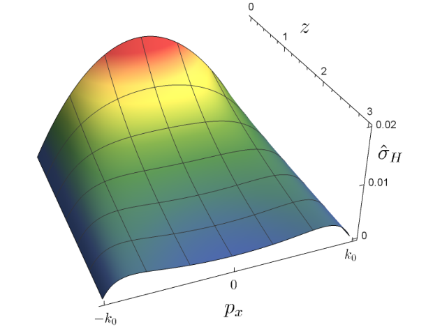
The current (III.13) at $\gamma=\pi/2$ is consistent with the following local conductivity of the surface state labelled by $p_{x}$:

$$\hat{\sigma}(p_{x},z)=\frac{e^{2}}{h}\frac{(p_{0}^{2}-p_{x}^{2}){\rm e}^{-z(p_{0}^{2}-p_{x}^{2})/p_{0}}}{2\pi p_{0}}\,,$$

(III.15)

independent of $\mu$. We plot $\hat{\sigma}(p_{x},z)$ for $\gamma=\pi/2$ in Fig. 4; its decay length in the bulk is given by $g(p_{x})^{-1}$: as expected, the states of the Fermi arc with $p_{x}$ approaching the Weyl point projections at $p_{x}=\pm p_{0}$ progressively penetrate deeper in the bulk and their contribution to the conductivity is weaker for $z=0$ but decays slower with the distance. For $p_{x}$ in the center of the Fermi arc, instead, the surface states are more localized and their contribution is stronger for $z=0$.

For generic values of the boundary condition parameter, the integrals in Eqs. (III.5) and (III.7) cannot be written in simple closed forms. The results simplify in the zero-temperature limit, that allows us to clearly evaluate the role of the boundary conditions and the chemical potential. For $T\to 0$ we can substitute the Fermi function (II.22) with:

$$f(\varepsilon;\beta,\mu)\stackrel{{\scriptstyle T\to 0}}{{\longrightarrow}}\Theta\left[\varepsilon\right]\Theta\left[\mu-\varepsilon\right]$$

(III.16)

Concerning the operators $n_{\rm s}$ and $j_{y}$ in Eqs. (III.5) and (III.7), in the limit $\mu_{s}\to 0$, the difference of the $T_{s}\to 0$ limits of the Fermi distributions in the integral is meant to return the contribution of the zero-energy Fermi arc states. From Eq. (III.8) we observe that the angle $\gamma$ fixes the direction of the surface current density in our model, which gets inverted for $\pi<\gamma<2\pi$. This inversion can be obtained in the physical systems only for Fermi arcs that connect the two projections of the Weyl points by winding across the Brillouin zone: our approximation of the lattice Hamiltonian (II.1), however, is accurate only for momenta relatively close to the Weyl points (and small values of $p_{0}$); therefore, Eq. (II.3) does not describe correctly the physics of the whole surface Brillouin zone, resulting in unbounded Fermi arcs for $\pi<\gamma<2\pi$.

The momentum integral in Eq. (III.5) determines the decay of the total density of the surface states in the bulk; in particular, for large values of $z$ we may approximate the density with the asymptotic expansion:

$$\left\langle n_{\rm s}(\bm{r})\right\rangle\approx\frac{\sqrt{p_{0}\left(p_{0}+2(\mu_{s}/v)\cos\gamma\right)}-p_{0}}{4\pi^{2}z^{2}\cos\gamma}\,.$$

(III.17)

This relation is defined only for $p_{0}+2(\mu_{s}/v)\cos\gamma>0$. For values of $\mu_{s}$ outside this range of validity, the surface states are either completely filled (for $\cos\gamma<0$) or completely empty (for $\cos\gamma>0$) and $\left\langle n_{\rm s}\right\rangle\approx-p_{0}/\left(4\pi^{2}z^{2}\cos\gamma\right)$. The relation (III.17) implies that the expectation value of the density and current density of the surface state decays as $z^{-2}$ in the bulk. As emphasized by several works gorbar16; resta18, this may yield in turn relevant scattering processes between surface and bulk states. The limit $z\to 0$, instead, provides an estimate of the surface density exactly at the boundary and it is given by:

$$\left\langle n_{\rm s}(z=0)\right\rangle=\frac{\sqrt{p_{0}}\left(p_{0}+2(\mu_{s}/v)\cos\gamma\right)^{5/2}-p_{0}^{3}}{15\pi^{2}\cos\gamma\sin^{2}\gamma}\,.$$

(III.18)

After defining $\hat{\sigma}(p_{x},z,\mu_{s})$ from Eq. (III.9), the integral in the $p_{x}$ momenta in Eq. (III.10) returns:

$$\sigma_{H}(z,\mu_{s})=\int dp_{x}\hat{\sigma}(p_{x})=\frac{e^{2}}{h}\frac{\sqrt{{p_{0}z\sin(\gamma)}}}{2\pi z^{2}}\times\\ \left\{\left[1+2{\tilde{p}_{0}}z\right]\,D_{+}\left(\sqrt{{\tilde{p}_{0}}z}\right)-\sqrt{{\tilde{p}_{0}}z}\,\right\},$$

(III.19)

where

$${\tilde{p}_{0}}=\frac{p_{0}+2(\mu_{s}/v)\cos(\gamma)}{\sin(\gamma)}\,.$$

(III.20)

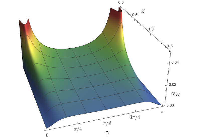
The conductance density (III.19) is represented in Fig. 5 as a function of the boundary condition parameter $\gamma$ and the distance from the surface $z$. It decays asymptotically as:

$$\sigma_{H}(z,\mu_{s})\approx\frac{e^{2}}{h}\frac{\sin\gamma}{2\pi z^{2}}\sqrt{\frac{p_{0}}{p_{0}+2(\mu_{s}/v)\cos(\gamma)}}\,.$$

(III.21)

All the previous results are based on the specific model (II.3) which is characterized by a single pair of Weyl cones and can be considered a good approximation for experimental systems with two Weyl cones only soh2019. In the case of materials with more Weyl points, however, we expect that each Fermi arc will provide a contribution to the anomalous Hall conductance given by the previous equations (III.19-III.15). The additivity of these contributions can be verified in the limit of small $p_{0}$, in which several pairs of Weyl points are sufficiently distant from each other in momentum space.

References

- (1) P. Hosur and X. Qi, Comp. Ren. Phys. 14, 857 (2013).
- (2) M. Z. Hasan, S.-Y. Xu, I. Belopolski and S.-M. Huang, Annu. Rev. Condens. Matter Phys. 8, 289 (2017).
- (3) B. Yan and C. Felser, Annu. Rev. Condens. Matter Phys. 8, 337 (2017).
- (4) A. A. Burkov, Annu. Rev. Condens. Matter Phys. 9, 359 (2018).
- (5) N. P. Armitage, E. J. Mele, and A.Vishwanath, Rev. Mod. Phys. 90, 015001 (2018).
- (6) B. Q. Lv, H. M. Weng, B. B. Fu, X. P. Wang, H. Miao, J. Ma, P. Richard, X. C. Huang, L. X. Zhao, G. F. Chen, Z. Fang, X. Dai, T. Qian, and H. Ding, Phys. Rev. X 5, 031013 (2015).
- (7) H. Weng, C. Fang, Z. Fang, B. A. Bernevig, and X. Dai, Phys. Rev. X 5, 011029 (2015).
- (8) S.-Y. Xu, N. Alidoust, I. Belopolski, C. Zhang, G. Bian, T.-R. Chang, H. Zheng, V. Strokov, D. S. Sanchez, G. Chang, Z. Yuan, D. Mou, Y. Wu, L. Huang, C.-C. Lee, S.-M. Huang, B. Wang, A. Bansil, H.-T. Jeng, T. Neupert, A. Kaminski, H. Lin, S. Jia, and M. Zahid Hasan, Nat. Phys. 11, 748 (2015).
- (9) S.-Y. Xu, I. Belopolski, D. S. Sanchez, C. Guo, G. Chang, C. Zhang, G. Bian, Z. Yuan, H. Lu, Y. Feng, T.-R. Chang, P. P. Shibayev, M. L. Prokopovych, N. Alidoust, H. Zheng, C.-C. Lee, S.-M. Huang, R. Sankar, F. Chou, C.-H. Hsu, H.-T. Jeng, A. Bansil, T. Neupert, V. N. Strocov, H. Lin, S. Jia, and M. Zahid Hasan, Sci. Adv. 1, 10 e1501092 (2015).
- (10) S.-Y. Xu, I. Belopolski, N. Alidoust, M. Neupane, C. Zhang, R. Sankar, S.-M. Huang, C.-C. Lee, G. Chang, B. Wang, G. Bian, H. Zheng, D. S. Sanchez, F. Chou, H. Lin, S. Jia, and M. Zahid Hasan, Science 349, 613 (2015).
- (11) X. Huang, L. Zhao, Y. Long, P. Wang, D. Chen, Z. Yang, H. Liang, M. Xue, H. Weng, Z. Fang, X. Dai, and G. Chen, Phys. Rev. X 5, 031023 (2015).
- (12) C.-L. Zhang et al., Nat. Commun. 7, 10735 (2016).
- (13) X. Wan, A. M. Turner, A. Vishwanath, and S. Y. Savrasov, Phys. Rev. B 83 205101 (2011).
- (14) A. A. Burkov and L. Balents, Phys. Rev. Lett. 107 127205 (2011).
- (15) A. A. Zyuzin and A. A. Burkov, Phys. Rev. B 86 115133 (2012).
- (16) K.-Y. Yang, Y.-M. Lu and Y. Ran, Phys. Rev. B 84, 075129 (2011).
- (17) H. B. Nielsen and M. Ninomiya, Phys. Lett. B 130 389 (1983).
- (18) P. Goswami and S. Tewari, Phys. Rev. B 88, 245107 (2013).
- (19) S. A. Parameswaran, T. Grover, D. A. Abanin, D. A. Pesin and A. Vishwanath, Phys. Rev. X 4, 031035 (2014).
- (20) Z.-M. Huang, J. Zhou and S.-Q. Shen, Phys. Rev. B 96, 085201 (2017).
- (21) L. Lepori, M. Burrello and E. Guadagnini, J. High Energy Phys. 2018, 110 (2018).
- (22) A. Ivashko, V. Cheianov and J. A. Hutasoit, arXiv:1802.00856 .
- (23) P. Baireuther, J. A. Hutasoit, J. Tworzydło and C. W. J. Beenakker, New J. Phys. 18, 045009 (2016).
- (24) D. Pesin, Nonlocal electrodynamics of helical metals, in Proceedings of 2016 IEEE International Conference on Mathematical Methods in Electromagnetic Theory (MMET), (IEEE, 2016) pp. 115–118.
- (25) A. Ivashko and V. Cheianov, arXiv:1712.05613
- (26) E. Witten, Nuovo Cimento 39, 313 (2016).
- (27) K. Hashimoto, T. Kimura and X. Wu, Prog. Theor. Exp. Phys. 2017, 053I01 (2017).
- (28) B. Seradjeh and M. Vennettilli, Phys. Rev. B 97, 075132 (2018).
- (29) Z. Faraei, T. Farajollahpour and S. A. Jafari, Phys. Rev. B 98, 195402 (2018).
- (30) E. V. Gorbar, V. A. Miransky, I. A. Shovkovy and P. O. Sukhachov, Phys. Rev. B 93, 235127 (2016).
- (31) G. Resta, S.-T. Pi, X. Wan and S. Y. Savrasov, Phys. Rev. B 97, 085142 (2018).
- (32) R.-J. Slager, V. Juričić and B. Roy, Phys. Rev. B 96, 201401(R) (2017).
- (33) H. B. Nielsen and M. Ninomiya, Phys. Lett. B 105 219 (1981).
- (34) J.-R. Soh, F. de Juan, M. G. Vergniory, N. B. M. Schröter, M. C. Rahn, D. Y. Yan, M. Bristow, P. A. Reiss, J. N. Blandy, Y. F. Guo, Y. G. Shi, T. K. Kim, A. McCollam, S. H. Simon, Y. Chen, A. I. Coldea, A. T. Boothroyd, arXiv:1901.10022.
- (35) R. Okugawa and S. Murakami, Phys. Rev. B 89, 235315 (2014).
- (36) J. Chesta Lopez, L. E. F. Foa Torres and A. S. Nunez, Phys. Rev. B 97, 125419 (2018).
- (37) S. Li and A. V. Andreev, Phys. Rev. B 92, 201107(R) (2015).
- (38) L. Lepori, I. C. Fulga, A. Trombettoni, and M. Burrello, Phys. Rev. B 94, 085107 (2016).
- (39) M. Reed and B. Simon, Methods of Modern Mathematical Physics II: Fourier Analysis, Self-Adjointness, (Academic Press, San Diego 1975).
- (40) E. McCann and V. I. Fal’ko, J. Phys. Condens. Matter 16, 2371 (2004).
- (41) A. Akhmerov and C. W. J. Beenakker, Phys. Rev. Lett. 98, 157003 (2007); Phys. Rev. B 77, 085423 (2008).
- (42) S. Souma, Z. Wang, H. Kotaka, T. Sato, K. Nakayama, Y. Tanaka, H. Kimizuka, T. Takahashi, K. Yamauchi, T. Oguchi, K. Segawa, and Y. Ando, Phys. Rev. B 93, 161112(R) (2016).
- (43) N. Morali, R. Batabyal, P. K. Nag, E. Liu, Q. Xu, Y. Sun, B. Yan, C. Felser, N. Avraham, and H. Beidenkopf, Science 365, 1286 (2019).
- (44) Z. Faraei and S. A. Jafari, Phys. Rev. B 100, 035447 (2019).
- (45) O. Bratteli and D. W. Robinson, Operator Algebras and Quantum Statistical Mechanics 2, (Springer, Berlin, 1996).
- (46) F. W. J. Olver, D. W. Lozier, R. F. Boisvert, C. W. Clark, NIST Handbook of Mathematical Functions, (Cambridge University Press, New York, 2010); L. Lewin, Polylogarithms and Associated Functions, (North-Holland, New York, 1981).
- (47) P. Baireuther, J. M. Edge, I. C. Fulga, C. W. J. Beenakker and J. Tworzydło, Phys. Rev. B 89, 035410 (2014).
- (48) J. Tworzydło, B. Trauzettel, M. Titov, A. Rycerz, and C. W. J. Beenakker, Phys. Rev. Lett. 96, 246802 (2006).
- (49) N. Bovenzi, M. Breitkreiz, T. E. O’Brien, J. Tworzydło and C. W. J. Beenakker, New J. Phys. 20 023023 (2018).
- (50) S. Tchoumakov, M. Civelli and M. O. Goerbig, Phys. Rev. B 95, 125306 (2017).
- (51) C. W. Groth, M. Wimmer, A. R. Akhmerov and X. Waintal, New J. Phys. 16, 063065 (2014). Software available at the webpage https://kwant-project.org.
- (52) V. Kaladzhyan and J. H. Bardarson, Phys. Rev. B 100, 085424 (2019).
- (53) S.-F. Zhang, C.-W. Zhang, P.-J. Wang and Q.-F. Sun, Sci. China Phys. Mech. Astron. 61, 117811 (2018).
- (54) F. C. Wellstood, C. Urbina and J. Clarke, Phys. Rev. B 49, 5942 (1994).
- (55) M. Banerjee, M. Heiblum, A. Rosenblatt, Y. Oreg, D. E. Feldman, A. Stern, and V. Umansky, Nature 545, 75 (2017).
- (56) R. Lundgren, P. Laurell and G. A. Fiete, Phys. Rev. B 90, 165115 (2014).
- (57) C. L. Kane and M. P. A. Fisher, Phys. Rev. B 55, 15832 (1997).
- (58) A. Cappelli, M. Huerta, and G. R. Zemba, Nucl. Phys. B 636, 568 (2002).
- (59) H. B. Callen, Thermodynamics and an Introduction to Thermostatistics, (John Wiley and Sons, New York 1960).
- (60) Y. Sun, S.-Ch. Wu and B. Yan, Phys. Rev. B 92, 115428 (2015).