Second-order topological phases protected by chiral symmetry
Abstract
We study second-order topological insulators and semimetals characterized by chiral symmetry. We investigate topological phase transitions of a model for construction of the two-dimensional second-order topological insulators protected only by chiral symmetry. By the theory of the phase transitions, we propose a second-order topological semimetal and insulators with flat hinge bands in chiral-symmetric three-dimensional systems. The three-dimensional second-order topological phases can be obtained from the stacked two-dimensional second-order topological insulators with chiral symmetry. Moreover, we show that broken chiral symmetry in the three-dimensional second-order topological phase allows a second-order topological insulator with chiral hinge states. We also demonstrate the second-order topological phases by using a lattice model.
I Introduction
Higher-order topological insulators have recently drawn research interest as new topological crystalline phases Benalcazar et al. 2017a; Benalcazar et al. 2017b; Song et al. 2017; Fang and Fu; Schindler et al. 2018a; Langbehn et al. 2017; Geier et al. 2018; Trifunovic and Brouwer 2019; Khalaf et al. 2018; Khalaf 2018; Matsugatani and Watanabe 2018; van Miert and Ortix 2018; Kooi et al. 2018; Wang et al. 2019; Ezawa 2018a; Ezawa 2018b; Ezawa 2018c; Ezawa 2018d; Ezawa 2018e; Ezawa 2019; Fukui and Hatsugai 2018; Kunst et al. 2018; Franca et al. 2018; Călugăru et al. 2019; Schindler et al. 2018b; Imhof et al. 2018; Serra-Garcia et al. 2018; Peterson et al. 2018; Ni et al. 2019; Fan et al. 2019; Ahn et al. 2019; Liu and Wakabayashi 2017; Liu et al. 2019; Rodriguez-Vega et al. 2019; Benalcazar et al. 2019; Wieder and Bernevig; Wieder et al. 2018; Hwang et al.. Unlike conventional first-order topological insulators, two-dimensional (2D) second-order topological insulators (SOTIs) have topologically protected corner states, and three-dimensional (3D) SOTIs have topological gapless modes on the hinges. In some crystalline SOTIs, the topological corner and hinge states can arise only from the nontrivial bulk topology, when the lattice termination is compatible with the crystal symmetries. The crystalline insulators with the nontrivial second-order topology, which are independent of the lattice termination, are called intrinsic second-order topological phases Langbehn et al. 2017; Geier et al. 2018; Trifunovic and Brouwer 2019.
Intriguingly, stacking 2D SOTIs enables the coexistence of topological gapless surface and hinge states while the bulk gap is open. The 3D SOTI can be realized by two anticommuting mirror symmetries Lin and Hughes 2018. Furthermore, the idea of the crystalline SOTIs has been extended to semimetallic phases, which are called second-order topological semimetals (SOTSMs) Lin and Hughes 2018; Wang et al. 2019; Ahn et al. 2018; Ezawa 2018a; Ezawa 2018b; Ezawa 2019; Călugăru et al. 2019; Wieder et al.. SOTSMs have not only topological hinge states but also topological gapless nodes in the bulk. The topological hinge states appear between the gapless points projected onto the hinges.
On the other hand, crystal symmetry is not necessarily required in order to realize SOTIs Seradjeh et al. 2008; Volovik 2010; Sitte et al. 2012; Zhang et al. 2013; Hashimoto et al. 2017; Li et al. 2018; Langbehn et al. 2017; Geier et al. 2018; Trifunovic and Brouwer 2019; Chen and Lado 2019; Bomantara et al. 2019; Hayashi 2018; Hayashi 2019. In this case, the topological classification of the -dimensional second-order topological phases is the same as that of the -dimensional first-order topological phases in the Altland-Zirnbauer classes Langbehn et al. 2017; Geier et al. 2018; Trifunovic and Brouwer 2019; Hayashi 2018; Hayashi 2019. The classification is based on the theory Langbehn et al. 2017; Geier et al. 2018; Trifunovic and Brouwer 2019; Hayashi 2018; Hayashi 2019, which means that the nontrivial phases are not fragile. Physically, the corner and hinge states are understandable as domain wall modes between topologically trivial and nontrivial boundaries Langbehn et al. 2017; Geier et al. 2018; Trifunovic and Brouwer 2019; Teo and Kane 2010. Thus, the SOTIs in the 3D class A and the 2D class AIII are characterized by invariants, which depend on the crystal termination. Such nontrivial phases are named extrinsic SOTIs Langbehn et al. 2017; Geier et al. 2018; Trifunovic and Brouwer 2019, whose topology of the corner (hinge) states is determined by both the bulk and the edges (surfaces). The SOTI phases are realizable even if we arbitrarily terminate the lattice Langbehn et al. 2017; Geier et al. 2018; Trifunovic and Brouwer 2019; Hayashi 2018; Hayashi 2019; Takane 2019. The topological modes are stable as long as the bulk and the boundary bands are gapped.
However, we need to calculate a complicated boundary Hamiltonian to study extrinsic second-order topology in general. The phase diagram to search for the SOTI is difficult to explore analytically without employing crystal symmetry. Thus, it is useful to give a systematic way to construct extrinsic SOTIs and the explicit topological invariant for the phase diagram. Moreover, topological gapless nodes are characterized by a change of topological invariants for lower-dimensional insulators in momentum space. Therefore, we can produce new 3D second-order topological phases from the phase diagram for the 2D SOTIs.
In this work, we show various second-order topological phases realized by chiral symmetry. We discuss a simple method to construct the chiral-symmetric second-order topological phases. To do so, we develop the previous method Hayashi 2018; Hayashi 2019 for the 2D SOTI protected only by chiral symmetry in view of the topological phase transition. From our theory, we also show different 3D second-order topological phases due to chiral symmetry, and one of them is an unconventional topological phase which has a single gapless point on the 2D surface in addition to the topological hinge states. Furthermore, it is found that the 3D SOTI with surface gapless points can become a 3D SOTI with chiral hinge states by broken chiral symmetry.
II Second-order topological phases characterized by chiral symmetry
In this section, we study SOTIs and a SOTSM characterized by chiral symmetry in terms of the bulk and edge gap closings for the topological phase transitions. We give a simple Hamiltonian to create the 2D SOTIs only by chiral symmetry and extend it to 3D systems by considering the translation symmetry.
II.1 Corner states and topological invariant
First of all, we review construction of 2D SOTIs in class AIII according to Ref. Hayashi 2018. We apply the method to 3D systems with chiral symmetry later. We consider the following bulk Hamiltonian:
| (1) |
where are two Hermitian matrices with chiral symmetry represented as . Here, , and is the identity matrix with the same size as . Because is satisfied, the Hamiltonian in Eq. (1) has chiral symmetry . In this paper, we focus on gap closing at zero energy because chiral symmetry is present. We impose open boundary condition (OBC) with a right-angled corner com. When the model is gapped at zero energy, it can be characterized by a topological invariant given by Hayashi 2018; Hayashi 2019
| (2) |
where are conventional winding numbers for . The expression of the winding number is given in the Appendix A. The winding numbers distinguish whether the one-dimensional (1D) bulk Hamiltonians are in the first-order topological phase by chiral symmetry Ryu and Hatsugai 2002; Schnyder et al. 2008; Ryu et al. 2010; Chiu et al. 2016. As discussed in the next section, is unchanged as long as the model is gapped at zero energy in the bulk and on the edges. The system with the nonzero is a 2D SOTI with zero-energy corner states.
Indeed, the nonzero indicates the existence of the corner states when the edges break the translation symmetries in the and the directions. We consider a semi-infinite system with one corner for Eq. (1). Because and are separate in Eq. (1), the real-space Hamiltonian can be described by two real-space Hamiltonians of and . We denote the Hamiltonians of as . The Hamiltonian under the corner boundary condition (CBC) can be represented as com
| (3) |
Here, and are representations of the chiral symmetry and the identity matrix in the terminated system, respectively. To see topological corner states, we assume that the bulk and the edges are gapped at zero energy. If both and are topologically nontrivial, i.e. , we can see the corner states with the zero energy as follows. Let be one of the topological zero-energy eigenvectors of at one zero-dimensional edge from the nonzero . Then, we can find a zero-energy state given by for in Eq. (3). By assumption, the zero-energy state should be a corner state. Generally, we can obtain topological corner states because have zero-energy modes. Thus, zero-energy corner states appear when is nonzero.
II.2 Topological phase transitions and gap closing
To grasp the 2D SOTI, we revisit the topological phase transitions in view of the gap closing. We clarify how the topological phases for change when we continuously deform . In other words, we can see how the band gap necessarily closes in the bulk or the edges when changes.
We assume that the system is in a trivial phase with to elucidate the topological phase transitions. and need to close the band gap to change . To begin with, we discuss the bulk gap given by Eq. (1). Because , the bulk Hamiltonian satisfies
| (4) |
Therefore, if and only if and take zero-valued eigenvalues at the same time, the bulk bands close the gap. This gap closing can change both and , and thus .
By contrast, can change even if and do not take zero-valued eigenvalues simultaneously. We consider a trivial phase with . From the above discussion, when the system enters a nontrivial phase with from the trivial phase, the bulk Hamiltonian does not close the band gap. Then, we investigate an edge normal to the direction. Namely, we see a semi-infinite system with the edge along the direction. Because we retain periodicity in the direction, the Hamiltonian under the edge boundary condition (EBC) can be described as
| (5) |
Although satisfies a condition similar to Eq. (4), we note that determines gap closing on the edge because has the nonzero . has the topological zero-mode now, and has Bloch eigenstates with the eigenvalues . Therefore, an eigenvector of the can be obtained from because it satisfies
| (6) |
can effectively describe the edge states near zero energy thanks to the nontrivial topology of . Hence, the gap closes on the edge when takes zero-valued eigenvalues.
We also analyze a topological phase transition from the phase with to the phase with . In this case, we show that gap closing happens on the edge normal to the direction. The Hamiltonian with the edge boundary is
| (7) |
Similarly, we can obtain an eigenstate of from due to the nonzero . is a Bloch function of . We can choose to satisfy because this state is a zero-energy mode of . Therefore, the gap closes on the edge through the eigenvalues of .
II.3 Construction of 3D SOTSMs and SOTIs
Hereafter, we generalize the theory about the 2D SOTI to 3D systems with chiral symmetry by adding translation symmetry in the direction. Since the wave vector is added to Eq. (1) in the 3D systems, the bulk Hamiltonian is given by
| (8) |
Thus, we can regard as a new parameter leading to the topological phase transition characterized by . The topological phase transition can occur in momentum space, in which gap-closing points can emerge due to the chiral symmetry for the 3D system. Therefore, the phase has the topological gap-closing points and hinge states at zero energy. As a result, we can realize a 3D second-order topological phase by stacking the 2D SOTIs.

The positions of the gapless points depend on how and give rise to the topological phase transitions. Because is periodic for , point nodes always appear in pairs. If and change the winding numbers and simultaneously, a SOTSM phase emerges in the bulk, as shown in Fig. 1(a). The system shows zero-energy hinge states between the nodes projected onto the hinges because of the nonzero . For example, the gapless node appears when changes from to in the 3D momentum space.
By contrast, the system can have gapless points on the surfaces. While the bulk is insulating, the surface gapless points coexist with topological hinge states. There are two types of topological phase transitions by the change in , which results in analogs of surface topological semimetals. We consider the first type where gapless points appear on the same surface. In this type, either or changes in momentum space while the other one is fixed to a nonzero value, for instance [Fig. 1(b)].
In the second type, we can obtain gapless points on the different surfaces. The point nodes can be found when and change in momentum space. We note that this surface gapless structure is unique to the 3D systems because 2D bulk topological semimetals necessarily have topological point nodes in pairs in momentum space Chiu et al. 2016; Matsuura et al. 2013; Zhao et al. 2016; Ahn and Yang 2017; Park and Yang 2017. As an example, each surface can have a single gapless point if changes as , as illustrated in Fig. 1(c). In both types, topological hinge states appear at the zero energy between the gapless points.
Next, we break chiral symmetry in the 3D SOTI with the gapless points on the surfaces. The gap opens at the point nodes because the symmetry protection is absent. Hence, we can discuss a surface Chern insulator due to massive Dirac cones Sitte et al. 2012; Zhang et al. 2013; Chen and Lado 2019; Haldane 1988. In the specific case, we can easily diagnose the existence of the gapless hinge states (see Appendix B). Typically, if the pairs become gapped by broken chiral symmetry, they can contribute to the surface Chern numbers. The chiral hinge states appear between the gapped surfaces on the trivial bulk. Consequently, the system can show the 3D SOTI phase with chiral symmetry breaking [Fig. 1(d)].
III Model
We study a lattice model to demonstrate the second-order topological phases realized by chiral symmetry, and confirm our theory in the previous section. The 2D lattice model is constructed from the Su-Schrieffer-Heeger (SSH) model Su et al. 1979, which can be transformed to the Benalcazar-Bernevig-Hughes model Benalcazar et al. 2017a; Benalcazar et al. 2017b.
III.1 The 2D SOTI model
We construct second-order topological phases and the Hamiltonian using the general method from Eq. (1). We study a 2D tight-binding model described as
| (9) |
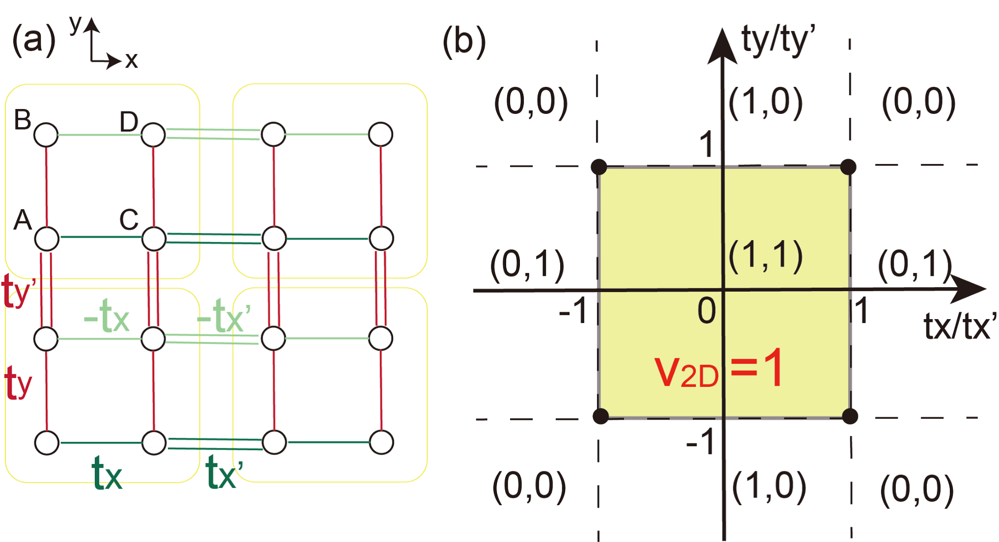
where and are the unit vectors in the and directions, respectively. and are real hopping parameters [see Fig. 2(a)]. We set the lattice constants to unity. The Hamiltonian in momentum space is
| (10) |
where and are Pauli matrices acting on the sublattices, and and are the identity matrices. The energy eigenvalues are
| (11) |
This model actually consists of the two SSH models represented by
| (12) |
and the chiral symmetry is given by
| (13) |
Thus, this 2D model has chiral symmetry .
The topological invariant can be calculated from the winding numbers for . They are given by
| (14) |
Hence, we can obtain the phase diagram for the 2D model from Eq. (2) [Fig. 2 (b)]. When the corner boundary condition is imposed and , the zero mode appears. In the Appendix C, we show the analytic eigenvector localized at the corner in this model.
We note that our model in Eq. (10) is topologically equivalent to the Benalcazar-Bernevig-Hughes model which can have topological corner modes protected by two anticommuting mirror symmetries Benalcazar et al. 2017a; Benalcazar et al. 2017b. Alternatively, we can reinterpret the zero-energy corner modes as a manifestation of the extrinsic second-order topology under the corner boundary condition in class AIII Hayashi 2019. Therefore, the corner modes can remain stable topologically even after the mirror symmetries are broken. We investigate the stability by breaking the crystal symmetries in Appendix D.
III.2 Stacked SOTI model
We stack the 2D SOTI model to demonstrate 3D second-order topological phases. While we preserve the chiral symmetry, we introduce terms depending on . The dependence on is determined by how the 2D SOTIs are stacked in the direction.
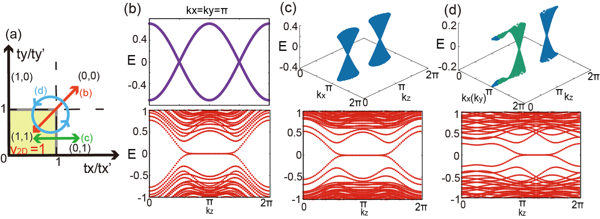
First, we add two terms and to the Hamiltonian in Eq. (10). These terms effectively alter the hopping terms and to and , respectively. Hence, the topological phase transition can happen in the momentum space. When and/or can be satisfied, the planes have gapless points.
Suppose that , and . In the parameter region, we can obtain a SOTSM with the bulk gapless points. If the parameters change as the red arrow in Fig. 3(a), two fourfold-degenerate points appear at in the bulk. The topological hinge states also exist between the projected point nodes, as shown in Fig. 3(b).
Next, we set to see a SOTI with gapless points on the surfaces. Since is fixed, only can change in momentum space. Therefore, we can realize gapless points on the surface perpendicular to the direction. For example, we change as the green arrow in the diagram. and change when . Figure 3(c) shows the two surface nodes at and the zero-energy hinge states between the two points projected to the hinges.
Second, we add the new terms, and , instead of the previous two terms. The hopping is effectively regarded as . If , the modified hoppings form the circle in the diagram, as depicted in Fig. 3(a). Thus, the gap closing can occur on the different surfaces when the circle encloses a phase transition point accompanied by bulk gap closing. We assume that the circle encloses the point , and that . Then, the point nodes appear at and on the surfaces normal to the and the directions, respectively [Fig. 3 (d)]. The anomalous distribution of the point nodes is allowed because the gap closings both in the bulk and on the surfaces change the hinge topology, similar to a mirror-symmetric topological quadrupolar semimetal Lin and Hughes 2018. To annihilate the surface point nodes, the gap should close in the bulk.
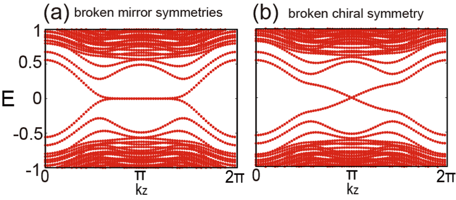
We emphasize that our Hamiltonian does not need any crystal symmetries to realize the second-order topological phases. The 2D chiral-symmetric model can also be characterized by the two mirror symmetries for quantization of the nested Wilson loop Benalcazar et al. 2017a; Benalcazar et al. 2017b; Lin and Hughes 2018. However, even if the mirror symmetries are broken, the hinge flat-band states can survive as long as the chiral symmetry exists. We can indeed see the protection of the chiral symmetry by breaking the mirror symmetries. For example, we introduce the term 2 for the case in Fig. 3(c). If , the topological zero-modes are stable because does not change [Fig. 4 (a)].
III.3 SOTIs with broken chiral symmetry
Finally, we break chiral symmetry to produce a 3D SOTI from the 3D SOTI with the surface gapless points. The system belongs to class A. By using our model, we here show that the SOTI can be realized easily from the surface gapless points in Fig. 3 (c). We add the perturbation in order to obtain the SOTI without chiral symmetry. Figure 4 (b) shows the gapless hinge states which originate from the zero-energy states.
To understand the topological phase transition, we investigate the surface normal to the direction from the discussion in Sec.II B. Because is topologically nontrivial, we can obtain the surface effective Hamiltonian near the zero energy by expanding (see also Appendix B). The effective Hamiltonian describes the surface Dirac points with the mass induced by the broken chiral symmetry.
We can calculate the surface Chern number from the surface Hamiltonian. The effective Hamiltonian near the gapless points is given by
| (15) |
where is the wave vector measured from . By the perturbation term, the Dirac cones at obtain the mass gap described as . Because and in the calculation, the surface has a Chern number of . As a result, the system becomes the SOTI phase, which is consistent with the discussion in Appendix B.
IV Conclusion and discussion
In the present paper, we have shown that various chiral-symmetric second-order topological insulators and semimetal are realizable. We have suggested the method to construct the second-order topological phases protected by chiral symmetry. The theory reveals that there are several types of chiral-symmetric second-order topological phases in three-dimensional systems, and that the topological phases can be obtained from stacked two-dimensional second-order topological insulators with chiral symmetry. The zero-energy hinge states are stable topologically by chiral symmetry. Particularly, we have discovered the second-order topological insulator, which has not only hinge bands but also a single gapless point on the surface thanks to chiral symmetry. In general, this surface gapless point is not allowed in the two-dimensional bulk because both the bulk and surfaces need to contribute topologically. We have also shown that broken chiral symmetry can yield the second-order topological insulator from the surface gapless points in the chiral-symmetric second-order topological insulators. Our method tells us how to give extrinsic second-order topology easily in classes A and AIII.
Importantly, if any Hamiltonian with chiral symmetry can be continuously deformed to Eq. (1) or (8) without the bulk and surface gap closings, we can distinguish whether the system has nontrivial second-order topology because the band topology is unchanged Hayashi 2018; Hayashi 2019. Namely, our theory is useful even though the Hamiltonian does not take the form in Eq. (1) or (8). Thus, our model is available for photonic and phononic crystals and electric circuits Imhof et al. 2018; Serra-Garcia et al. 2018; Peterson et al. 2018; Ni et al. 2019; Fan et al. 2019 because their structures are flexibly controllable. Theoretically, corner modes in class BDI are suggested in photonic systems composed of waveguides and of coupled ring resonators with negative hopping amplitudes Li et al. 2018. We also expect that our second-order topological phases can be constructed in waveguide arrays, and that the corner modes are detectable through measurement of the outgoing intensity distribution of light injected into a waveguide. Moreover, electric circuits have the possibility of experimental realization of the second-order topological phases protected by chiral symmetry, because capacitors and inductors can provide band structures of the circuit Laplacian Imhof et al. 2018; Lee et al. 2018; Helbig et al. 2019. The nontrivial second-order topological modes in the electric circuits are measurable by the impedance response since the zero modes contribute to large resonances at the boundaries such as corners. Therefore, our model is feasible in systems with the easily controllable structures.
Additionally, topological stability of gapless nodes is characterized locally by the change of a topological invariant in momentum space Chiu et al. 2016; Matsuura et al. 2013; Zhao et al. 2016. Therefore, the nodal structures in our paper are allowed in other classes with chiral symmetry. Actually, second-order topological phases have been predicted in superconductors Langbehn et al. 2017; Geier et al. 2018; Trifunovic and Brouwer 2019; Khalaf 2018; Shapourian et al. 2018; Zhu 2018; Yan et al. 2018; Wang et al. 2018a; Wang et al. 2018b; Hsu et al. 2018; Liu et al. 2018; Bultinck et al. 2019; Wu et al. 2019; Zhang et al. 2019; Peng and Xu 2019; Ghorashi et al. 2019. Some of the topological superconductors are understandable in view of extrinsic second-order topology Peng and Xu 2019; Ghorashi et al. 2019. Recently, robust Majorana hinge states were studied in a second-order topological superconductor as long as the particle-hole symmetry is preserved Ghorashi et al. 2019. Thus, the extrinsic second-order topological nodal phases protected by chiral symmetry are expected to appear in superconductors with time-reversal symmetry.
Acknowledgements.
We are grateful to R. Takahashi and S. Murakami for helpful discussion. This work is supported by World Premier International Research Center Initiative (WPI), MEXT, Japan, JPSJ Grant-in-Aid Scientific Research on Innovative Areas “Discrete Geometric Analysis for Materials Design” (Grant No. 17H06460 and No. 17H06461), and JSPS KAKENHI Grants No. JP19K14545 and No. 16K05412, and JST-CREST (JPMJCR18T1), and JST-PRESTO (JPMJPR19L7).Appendix A Expression of the winding number
To describe the topological invariant in a self-contained way, we explicitly write the winding number for the 1D Hamiltonian with chiral symmetry. To do so, we introduce the following matrix:
| (16) |
where the sum is taken over the eigenstates below zero energy. In the basis where the chiral symmetry is diagonal, the matrix can be rewritten as
| (17) |
By using the off-diagonal component , the winding number is defined as Schnyder et al. 2008; Ryu et al. 2010; Chiu et al. 2016
| (18) |
The winding number corresponds to the number of topological edge states in the 1D chiral-symmetric system.
Appendix B Model for chiral hinge states
In this appendix, we give a 3D Hamiltonian which shows chiral hinge states without the protection of any symmetries. The Hamiltonian is beneficial to obtain the 3D extrinsic SOTI in class A. We consider the following bulk Hamiltonian Hayashi 2018:
| (19) |
Here, is a Hermitian matrix without symmetry, and has the same size as . is the chiral-symmetric Hamiltonian explained in Sec. II. We assume that the bulk and the surface gaps are open at zero energy. Because Eqs. (19) and (1) have the same structure, we discuss the topological hinge states in a manner similar to Sec. II by regarding as a 2D bulk Hamiltonian. Therefore, we define a Chern number for , which gives the 1D chiral edge states . The Chern number is defined for the bulk bands below zero energy since the origin of the energy can be shifted.
To see chiral hinge states in the 3D SOTI, we investigate the semi-infinite Hamiltonian with one hinge:
| (20) |
We maintain the translation symmetry in the direction. In the same way as in Sec. II, we can obtain topological hinge states with the gapless dispersion if and are nonzero. Thus, we can introduce a topological invariant , which characterizes the number of gapless hinge states Hayashi 2018. Realistically, can depend on . However, since can be interpreted as a parameter in , gapless hinge states can be detected if the model can be adiabatically deformed to Eq. (19) .
In comparison with our model in Sec. III C, is given by . The massive Dirac cones on the surface give the nonzero Chern number . As a result, we obtain the chiral hinge states from the SOTI with the broken chiral symmetry.
On the other hand, the phase transition from a SOTSM to a SOTI with chiral hinge states was also suggested in 3D systems with parity symmetry Wang et al. 2019; Ahn et al. 2018. The SOTSM hosts nodal lines topologically protected by parity-time symmetry in pairs, giving nearly flat hinge bands between the nodal lines. Time-reversal symmetry breaking in the SOTSM realizes the 3D SOTI, and the nearly flat hinge states become the chiral hinge states in the SOTI. The chiral hinge states are intrinsically protected by the parity symmetry Wang et al. 2019; Ahn et al. 2018; Geier et al. 2018; Khalaf et al. 2018; Khalaf 2018. By contrast, our topological phase transition stems from broken chiral symmetry, and the induced chiral hinge states are characterized by the extrinsic second-order topology.
Appendix C Zero-energy states of the models
For the model in Eq. (9), we can analytically compute the topological zero-energy eigenstate. Thus, we can see how the zero-energy modes are localized. The eigenstate can be obtained from zero modes of the SSH model. Thus, we focus on the SSH model corresponding to in Eq. (10), which is topologically nontrivial if . Let us label positions of the unit cell as in the 2D semi-infinite real space with one corner [see also Fig. 2(a)]. Since we can separately calculate the two SSH models in our model, we denote components of the eigenvector to represent the -th unit cell with the two sublattices as . The boundary condition is given by .
The components of the zero-mode satisfy
| (21) |
We can find the solution which decays as becomes larger when . From Eqs. (21), the solution is
| (22) |
Thus, the zero-energy state for Eq. (9) can be obtained from
| (23) |
Hence, the zero-energy mode is exponentially localized at the corner.
We can also describe zero-energy states of the 3D second-order topological phases in Sec. III C. We give the hopping parameters dependence, and write them as . The 3D model hosts the topological flat band if and . Since the system is periodic in the direction, we can consider the zero modes by fixing and replacing with in Eq. (23). As a result, we can see that the zero modes are localized at the hinge. When and/or , the hinge flat band merges into the correspondent gapless points.
Appendix D Topological stability of the corner modes without protection of crystal symmetries
Our 2D SOTI Hamiltonian in Eq. (4) does not need protection of crystal symmetries thanks to the chiral symmetry. Here, we show the topological stability of the corner modes by breaking crystal symmetries in the model in Eq. (9). This also describes the robustness of hinge states in the 3D chiral-symmetric second-order nontrivial phases, although the translation symmetry is necessary for the dependence. Because the hinge states are characterized locally in momentum space by , we can understand them as corner modes in the 2D chiral-symmetric SOTI parametrized by . Therefore, we focus on the corner modes in the 2D SOTIs.
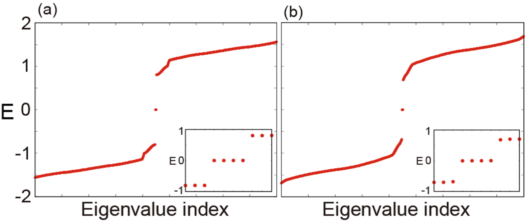
The chiral-symmetric model has twofold-rotational symmetry, and two mirror symmetries with respect to the and the axis if and in addition to time-reversal and particle hole symmetries. To break the symmetries except the chiral symmetry, we add a perturbation term, in Eq. (9), where the summation of and runs over sublattices , , , and . The perturbation preserves the chiral symmetry. Unless the additional term closes the bulk and edge gaps in the nontrivial phase, the corner modes are robust even if the Hamiltonian does not have the form in Eq. (1). Figure 5 shows topological corner modes in the model. As shown in Fig. 5(b), the corner modes survive after the perturbation breaking the crystal symmetries is added. Hence, we can see the topological stability of the corner modes due to the chiral symmetry.
References
- Benalcazar et al. (2017a) W. A. Benalcazar, B. A. Bernevig, and T. L. Hughes, Science 357, 61 (2017a).
- Benalcazar et al. (2017b) W. A. Benalcazar, B. A. Bernevig, and T. L. Hughes, Phys. Rev. B 96, 245115 (2017b).
- Song et al. (2017) Z. Song, Z. Fang, and C. Fang, Phys. Rev. Lett. 119, 246402 (2017).
- (4) C. Fang and L. Fu, arXiv:1709.01929 .
- Schindler et al. (2018a) F. Schindler, A. M. Cook, M. G. Vergniory, Z. Wang, S. S. Parkin, B. A. Bernevig, and T. Neupert, Sci. Adv. 4, eaat0346 (2018a).
- Langbehn et al. (2017) J. Langbehn, Y. Peng, L. Trifunovic, F. von Oppen, and P. W. Brouwer, Phys. Rev. Lett. 119, 246401 (2017).
- Geier et al. (2018) M. Geier, L. Trifunovic, M. Hoskam, and P. W. Brouwer, Phys. Rev. B 97, 205135 (2018).
- Trifunovic and Brouwer (2019) L. Trifunovic and P. W. Brouwer, Phys. Rev. X 9, 011012 (2019).
- Khalaf et al. (2018) E. Khalaf, H. C. Po, A. Vishwanath, and H. Watanabe, Phys. Rev. X 8, 031070 (2018).
- Khalaf (2018) E. Khalaf, Phys. Rev. B 97, 205136 (2018).
- Matsugatani and Watanabe (2018) A. Matsugatani and H. Watanabe, Phys. Rev. B 98, 205129 (2018).
- van Miert and Ortix (2018) G. van Miert and C. Ortix, Phys. Rev. B 98, 081110(R) (2018).
- Kooi et al. (2018) S. H. Kooi, G. van Miert, and C. Ortix, Phys. Rev. B 98, 245102 (2018).
- Wang et al. (2019) Z. Wang, B. J. Wieder, J. Li, B. Yan, and B. A. Bernevig, Phys. Rev. Lett. 123, 186401 (2019).
- Ezawa (2018a) M. Ezawa, Phys. Rev. B 97, 155305 (2018a).
- Ezawa (2018b) M. Ezawa, Phys. Rev. Lett. 120, 026801 (2018b).
- Ezawa (2018c) M. Ezawa, Phys. Rev. Lett. 121, 116801 (2018c).
- Ezawa (2018d) M. Ezawa, Phys. Rev. B 97, 241402(R) (2018d).
- Ezawa (2018e) M. Ezawa, Phys. Rev. B 98, 045125 (2018e).
- Ezawa (2019) M. Ezawa, Scientific reports 9, 5286 (2019).
- Fukui and Hatsugai (2018) T. Fukui and Y. Hatsugai, Phys. Rev. B 98, 035147 (2018).
- Kunst et al. (2018) F. K. Kunst, G. van Miert, and E. J. Bergholtz, Phys. Rev. B 97, 241405(R) (2018).
- Franca et al. (2018) S. Franca, J. van den Brink, and I. C. Fulga, Phys. Rev. B 98, 201114(R) (2018).
- Călugăru et al. (2019) D. Călugăru, V. Juričić, and B. Roy, Phys. Rev. B 99, 041301(R) (2019).
- Schindler et al. (2018b) F. Schindler, Z. Wang, M. G. Vergniory, A. M. Cook, A. Murani, S. Sengupta, A. Y. Kasumov, R. Deblock, S. Jeon, I. Drozdov, et al., Nat. Phys. 14, 918 (2018b).
- Imhof et al. (2018) S. Imhof, C. Berger, F. Bayer, J. Brehm, L. W. Molenkamp, T. Kiessling, F. Schindler, C. H. Lee, M. Greiter, T. Neupert, et al., Nat. Phys. 14, 925 (2018).
- Serra-Garcia et al. (2018) M. Serra-Garcia, V. Peri, R. Süsstrunk, O. R. Bilal, T. Larsen, L. G. Villanueva, and S. D. Huber, Nature 555, 342 (2018).
- Peterson et al. (2018) C. W. Peterson, W. A. Benalcazar, T. L. Hughes, and G. Bahl, Nature 555, 346 (2018).
- Ni et al. (2019) X. Ni, M. Weiner, A. Alù, and A. B. Khanikaev, Nat. Mater. 18, 113 (2019).
- Fan et al. (2019) H. Fan, B. Xia, L. Tong, S. Zheng, and D. Yu, Phys. Rev. Lett. 122, 204301 (2019).
- Ahn et al. (2019) J. Ahn, S. Park, and B.-J. Yang, Phys. Rev. X 9, 021013 (2019).
- Liu and Wakabayashi (2017) F. Liu and K. Wakabayashi, Phys. Rev. Lett. 118, 076803 (2017).
- Liu et al. (2019) F. Liu, H.-Y. Deng, and K. Wakabayashi, Phys. Rev. Lett. 122, 086804 (2019).
- Rodriguez-Vega et al. (2019) M. Rodriguez-Vega, A. Kumar, and B. Seradjeh, Phys. Rev. B 100, 085138 (2019).
- Benalcazar et al. (2019) W. A. Benalcazar, T. Li, and T. L. Hughes, Phys. Rev. B 99, 245151 (2019).
- (36) B. J. Wieder and B. A. Bernevig, arXiv:1810.02373 .
- Wieder et al. (2018) B. J. Wieder, B. Bradlyn, Z. Wang, J. Cano, Y. Kim, H.-S. D. Kim, A. M. Rappe, C. Kane, and B. A. Bernevig, Science 361, 246 (2018).
- (38) Y. Hwang, J. Ahn, and B.-J. Yang, arXiv:1905.08128 .
- Lin and Hughes (2018) M. Lin and T. L. Hughes, Phys. Rev. B 98, 241103(R) (2018).
- Ahn et al. (2018) J. Ahn, D. Kim, Y. Kim, and B.-J. Yang, Phys. Rev. Lett. 121, 106403 (2018).
- (41) B. J. Wieder, Z. Wang, J. Cano, X. Dai, L. M. Schoop, B. Bradlyn, and B. A. Bernevig, arXiv:1908.00016 .
- Seradjeh et al. (2008) B. Seradjeh, C. Weeks, and M. Franz, Phys. Rev. B 77, 033104 (2008).
- Volovik (2010) G. E. Volovik, JETP Lett. 91, 201 (2010).
- Sitte et al. (2012) M. Sitte, A. Rosch, E. Altman, and L. Fritz, Phys. Rev. Lett. 108, 126807 (2012).
- Zhang et al. (2013) F. Zhang, C. L. Kane, and E. J. Mele, Phys. Rev. Lett. 110, 046404 (2013).
- Hashimoto et al. (2017) K. Hashimoto, X. Wu, and T. Kimura, Phys. Rev. B 95, 165443 (2017).
- Li et al. (2018) L. Li, M. Umer, and J. Gong, Phys. Rev. B 98, 205422 (2018).
- Chen and Lado (2019) W. Chen and J. L. Lado, Phys. Rev. Lett. 122, 016803 (2019).
- Bomantara et al. (2019) R. W. Bomantara, L. Zhou, J. Pan, and J. Gong, Phys. Rev. B 99, 045441 (2019).
- Hayashi (2018) S. Hayashi, Commun. Math. Phys. 364, 343 (2018).
- Hayashi (2019) S. Hayashi, Lett. Math. Phys. 109, 2223 (2019).
- Teo and Kane (2010) J. C. Y. Teo and C. L. Kane, Phys. Rev. B 82, 115120 (2010).
- Takane (2019) Y. Takane, Journal of the Physical Society of Japan 88, 094712 (2019).
- (54) We especially use superscripts ,and for the Hamiltonians when the corner, edge, and hinge boundary conditions are imposed, respectively .
- Ryu and Hatsugai (2002) S. Ryu and Y. Hatsugai, Phys. Rev. Lett. 89, 077002 (2002).
- Schnyder et al. (2008) A. P. Schnyder, S. Ryu, A. Furusaki, and A. W. W. Ludwig, Phys. Rev. B 78, 195125 (2008).
- Ryu et al. (2010) S. Ryu, A. P. Schnyder, A. Furusaki, and A. W. W. Ludwig, New J. Phys. 12, 065010 (2010).
- Chiu et al. (2016) C.-K. Chiu, J. C. Y. Teo, A. P. Schnyder, and S. Ryu, Rev. Mod. Phys. 88, 035005 (2016).
- Matsuura et al. (2013) S. Matsuura, P.-Y. Chang, A. P. Schnyder, and S. Ryu, New J. Phys. 15, 065001 (2013).
- Zhao et al. (2016) Y. X. Zhao, A. P. Schnyder, and Z. D. Wang, Phys. Rev. Lett. 116, 156402 (2016).
- Ahn and Yang (2017) J. Ahn and B.-J. Yang, Phys. Rev. Lett. 118, 156401 (2017).
- Park and Yang (2017) S. Park and B.-J. Yang, Phys. Rev. B 96, 125127 (2017).
- Haldane (1988) F. D. M. Haldane, Phys. Rev. Lett. 61, 2015 (1988).
- Su et al. (1979) W. P. Su, J. R. Schrieffer, and A. J. Heeger, Phys. Rev. Lett. 42, 1698 (1979).
- Lee et al. (2018) C. H. Lee, S. Imhof, C. Berger, F. Bayer, J. Brehm, L. W. Molenkamp, T. Kiessling, and R. Thomale, Communications Physics 1, 39 (2018).
- Helbig et al. (2019) T. Helbig, T. Hofmann, C. H. Lee, R. Thomale, S. Imhof, L. W. Molenkamp, and T. Kiessling, Phys. Rev. B 99, 161114(R) (2019).
- Shapourian et al. (2018) H. Shapourian, Y. Wang, and S. Ryu, Phys. Rev. B 97, 094508 (2018).
- Zhu (2018) X. Zhu, Phys. Rev. B 97, 205134 (2018).
- Yan et al. (2018) Z. Yan, F. Song, and Z. Wang, Phys. Rev. Lett. 121, 096803 (2018).
- Wang et al. (2018a) Y. Wang, M. Lin, and T. L. Hughes, Phys. Rev. B 98, 165144 (2018a).
- Wang et al. (2018b) Q. Wang, C.-C. Liu, Y.-M. Lu, and F. Zhang, Phys. Rev. Lett. 121, 186801 (2018b).
- Hsu et al. (2018) C.-H. Hsu, P. Stano, J. Klinovaja, and D. Loss, Phys. Rev. Lett. 121, 196801 (2018).
- Liu et al. (2018) T. Liu, J. J. He, and F. Nori, Phys. Rev. B 98, 245413 (2018).
- Bultinck et al. (2019) N. Bultinck, B. A. Bernevig, and M. P. Zaletel, Phys. Rev. B 99, 125149 (2019).
- Wu et al. (2019) Z. Wu, Z. Yan, and W. Huang, Phys. Rev. B 99, 020508(R) (2019).
- Zhang et al. (2019) R.-X. Zhang, W. S. Cole, and S. Das Sarma, Phys. Rev. Lett. 122, 187001 (2019).
- Peng and Xu (2019) Y. Peng and Y. Xu, Phys. Rev. B 99, 195431 (2019).
- Ghorashi et al. (2019) S. A. A. Ghorashi, X. Hu, T. L. Hughes, and E. Rossi, Phys. Rev. B 100, 020509(R) (2019).