跳到论文正文
W Papers独立论文阅读器 arXiv:1907.01089 论文正文 计算阅读时间 · 0%
引用这篇论文根据当前论文元数据生成,正式投稿前建议核对。


License: arXiv.org perpetual non-exclusive license
arXiv:1907.01089v2 [math.DS] 11 Feb 2021

 Robust degenerate unfoldings of cycles and tangencies

Pablo G. Barrientos Address: Instituto de Matemática e Estatística, UFF
Rua Mário Santos Braga s/n - Campus Valonguinhos, Niterói, Brazil
Email address: pgbarrientos@id.uff.br
and Artem Raibekas Address: Instituto de Matemática e Estatística, UFF
Rua Mário Santos Braga s/n - Campus Valonguinhos, Niterói, Brazil
Email address: artem@mat.uff.br
Abstract.

We construct open sets of degenerate unfoldings of heterodimensional cycles of any co-index c>0c>0 and homoclinic tangencies of arbitrary codimension c>0c>0. These type of sets are known to be the support of unexpected phenomena in families of diffeomorphisms, such as the Kolmogorov typical co-existence of infinitely many attractors. As a prerequisite, we also construct robust homoclinic tangencies of large codimension which cannot be inside a strong partially hyperbolic set.

Key words and phrases: 
Homoclinic tangencies, heterodimensional cycle, blenders, parablenders
2010 Mathematics Subject Classification
Primary 58F15, 58F17; Secondary: 53C35.

1. Introduction

Robust homoclinic tangencies and robust heterodimensional cycles are, in general, prerequisites for obtaining abundant complicated dynamical systems [New70, GŠ72, New74, BD08, BD12]. Both configurations imply the existence of a non-transversal intersection between the stable and unstable manifolds of points in the same or in different transitive hyperbolic sets. A priori, the non-transverse intersection could be destroyed by a small perturbation. But since it is robust, this means that a new non-transverse intersection is created between the manifolds of the continuation of the hyperbolic sets. The unfolding of these bifurcations yields a great number of changes in the dynamics. For instance, infinitely many saddle periodic points and sinks appear in the unfolding of homoclinic tangencies. Hence, the persistence of these bifurcations allowed to get a generic coexistence of infinitely many periodic attractors [New79, GTS93, PV94, GST08].

The construction of robust tangencies in lower dimension is based on the creation of thick horseshoes involving distortion estimates which are typically C2C^{2}. However, in higher dimensions it was possible to construct robust homoclinic tangencies in the C1C^{1}-topology using blenders [Asa08, BD12]. Blenders are hyperbolic sets having a thicker invariant manifold than initially expected. They were discovered by Bonatti and Diaz [BD96] and now are essential objects in the study of non-hyperbolic dynamics. On the other hand, all of the above mentioned constructions are of codimension one. That is, the dimension of the coincidence of the tangent spaces at the tangent point. Recently in [BR17], the authors gave the first examples of C2C^{2}-robust tangencies of large codimension. The novelty in the construction was the use of the blender for the dynamics induced in the tangent bundle.

A different approach, when compared to the generic results mentioned above, is to look for bifurcations of homoclinic tangencies in parametric families of diffeomorphisms. For decades it was thought that the coexistence of infinitely many hyperbolic attractors was meager in families of dynamical systems [PS96]. However, recently and far from intuition, Berger showed in [Ber16] that actually these phenomena form a residual set. Behind this result was the construction of open sets of families of endomorphisms with robust homoclinic tangencies and with an extra property: the family unfolds degenerately a tangency. This means the unfolding is slow in the sense of the zeroing of the first terms in a certain Taylor polynomial describing the local separation between the manifolds. Although a degenerate unfolding of a tangency could be destroyed by a small perturbation of the family, this perturbation has another tangency which unfolds also degenerately. The mechanism involved in these constructions of Berger [Ber16] is also the blender, but now constructed for the dynamics induced in the space of jets (the space of velocities). See also [BCP16, Ber17a].

The objective of the present work is to unite the construction of [BR17] and [Ber16] to obtain robust degenerate unfoldings of homoclinic tangencies of large codimension for families of diffeomorphisms. Only this will not be done by merely combining the two previous results. Here we present a new method of construction of robust tangencies of large codimension, different from the one in [BR17]. This is a generalization to higher codimension of the construction in [BD12] using folding manifolds. It is expected that the unfolding of these robust degenerated tangencies gives new dynamical consequences. For example, the existence of residual sets with infinitely many attracting invariant tori of large dimension.

1.1. Dimension and codimension of an intersection

Let us begin with some definitions on the intersections of submanifolds. Let ℒ\mathcal{L} and 𝒮\mathcal{S} be submanifolds of ℳ\mathcal{M}. We say that ℒ\mathcal{L} and 𝒮\mathcal{S} have an intersection of dimension d≥0d\geq 0 at x∈ℒ∩𝒮x\in\mathcal{L}\cap\mathcal{S}, if

d=dx​(ℒ,𝒮)=defdimTx​ℒ∩Tx​𝒮.d=d_{x}(\mathcal{L},\mathcal{S})\stackrel{{\scriptstyle\scriptscriptstyle\rm def}}{{=}}\dim T_{x}\mathcal{L}\cap T_{x}\mathcal{S}.

Notice that dd is the maximum number of common linearly independent tangent directions in Tx​ℳT_{x}\mathcal{M}. However, this number is not enough to measure how far the intersection is from being transverse. In order to quantify this we say that ℒ\mathcal{L} and 𝒮\mathcal{S} have an intersection of codimension c≥0c\geq 0 if

c=cx​(ℒ,𝒮)=defdimℳ−dim(Tx​ℒ+Tx​𝒮).c=c_{x}(\mathcal{L},\mathcal{S})\stackrel{{\scriptstyle\scriptscriptstyle\rm def}}{{=}}\dim\mathcal{M}-\dim\left(T_{x}\mathcal{L}+T_{x}\mathcal{S}\right).

An intersection of codimension zero is called transverse and is said to be tangencial otherwise. Observe that the definition of a tangency (c>0c>0) includes the case d=0d=0 in which Tx​ℒ+Tx​𝒮=Tx​ℒ⊕Tx​𝒮T_{x}\mathcal{L}+T_{x}\mathcal{S}=T_{x}\mathcal{L}\oplus T_{x}\mathcal{S}. In the literature this case is called as a quasi-transverse intersection. On the other hand, the sum of the dimension and the codimension of an intersection between submanifolds is in general not equal to the dimension of ℳ\mathcal{M}. Moreover, when the codimension of ℒ\mathcal{L} coincides with the dimension of 𝒮\mathcal{S}, then if x∈ℒ∩𝒮x\in\mathcal{L}\cap\mathcal{S}

cx​(ℒ,𝒮)=dimℳ−(dimTx​ℒ+dimTx​𝒮−dimTx​ℒ∩Tx​𝒮)=dx​(ℒ,𝒮).c_{x}(\mathcal{L},\mathcal{S})=\dim\mathcal{M}-(\dim T_{x}\mathcal{L}+\dim T_{x}\mathcal{S}-\dim T_{x}\mathcal{L}\cap T_{x}\mathcal{S})=d_{x}(\mathcal{L},\mathcal{S}).
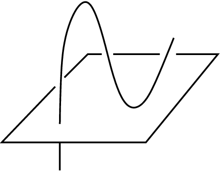
Refer to caption
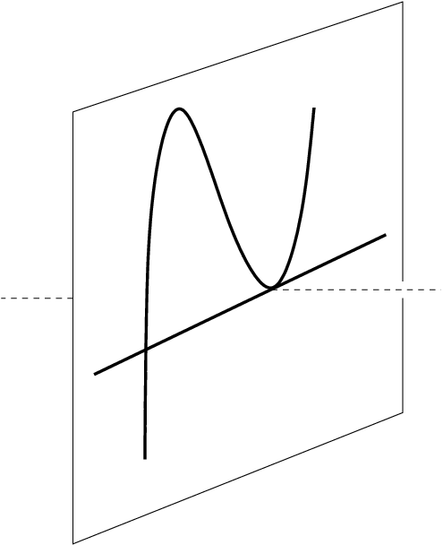
Refer to caption
Figure 1. Intersection of two submanifolds in a three dimensional space. Figure 1 shows a transverse intersection at the point x1x_{1} and a tangency of codimension c=1c=1 at x2x_{2} (and dimension also d=1d=1). Figure 1 shows intersections of codimension c=1c=1 and c=2c=2 at y1y_{1} and y2y_{2} respectively. At y1y_{1} we have a quasi-transverse intersection (dimension d=0d=0) and at y2y_{2} we have a tangency of dimension d=1d=1.

1.2. Heterodimensional cycles and homoclinic tangencies

A CrC^{r}-diffeomorphism ff of a manifold ℳ\mathcal{M} has a homoclinic tangency of codimension c>0c>0 if there is a pair of points PP and QQ, in the same transitive hyperbolic set, so that the unstable invariant manifold of PP and the stable invariant manifold of QQ have an intersection of codimension cc at a point YY. That is,

Y∈Wu​(P)∩Ws​(Q)andc=cY​(Wu​(P),Ws​(Q)).Y\in W^{u}(P)\cap W^{s}(Q)\quad\text{and}\quad c=c_{Y}(W^{u}(P),W^{s}(Q)).

Observe that actually, as the codimension of Wu​(P)W^{u}(P) coincides with the dimension of Ws​(Q)W^{s}(Q) we have that also in this case

c=dY​(Wu​(P),Ws​(Q)).c=d_{Y}(W^{u}(P),W^{s}(Q)).

Similarly, ff has a heterodimensional cycle of co-index c>0c>0 if there exist two transitive hyperbolic sets Λ\Lambda and Γ\Gamma such that their invariant manifolds meet cyclically and |inds​(Λ)−inds​(Γ)|=c|\mathrm{ind}^{s}(\Lambda)-\mathrm{ind}^{s}(\Gamma)|=c. Here inds​(⋅)\mathrm{ind}^{s}(\cdot) denotes the dimension of the stable bundle of the respective set. By means of an arbitrarily small perturbation if necessary, the stable and unstable manifolds have a transverse intersection of dimension cc and a tangency which is a quasi-transverse intersection of codimension cc. Indeed, we can assume that inds​(Λ)−inds​(Γ)=c\mathrm{ind}^{s}(\Lambda)-\mathrm{ind}^{s}(\Gamma)=c and for P∈ΛP\in\Lambda, Q∈ΓQ\in\Gamma suppose that YY belongs to Ws​(P)∩Wu​(Q)W^{s}(P)\cap W^{u}(Q). Then dimTY​Ws​(P)+dimTY​Wu​(Q)=dimℳ+c\dim T_{Y}W^{s}(P)+\dim T_{Y}W^{u}(Q)=\dim\mathcal{M}+c and thus, in general,

dY​(Ws​(P),Wu​(Q))=candcY​(Ws​(P),Wu​(Q))=0.d_{Y}(W^{s}(P),W^{u}(Q))=c\quad\text{and}\quad c_{Y}(W^{s}(P),W^{u}(Q))=0.

On the other hand, if Y∈Wu​(P)∩Ws​(Q)Y\in W^{u}(P)\cap W^{s}(Q) then dimTY​Wu​(P)+dimTY​Ws​(Q)=dimℳ−c\dim T_{Y}W^{u}(P)+\dim T_{Y}W^{s}(Q)=\dim\mathcal{M}-c and hence,

dY​(Wu​(P),Ws​(Q))=0andcY​(Wu​(P),Ws​(Q))=c.d_{Y}(W^{u}(P),W^{s}(Q))=0\quad\text{and}\quad c_{Y}(W^{u}(P),W^{s}(Q))=c.

1.3. Robust tangencies of large codimension

By Kupka-Smale’s theorem, CrC^{r}-generically, the stable and unstable manifolds of a pair of saddle hyperbolic periodic points meet transversally. Hence, tangencies associated with saddles occurs in the complement of a residual set of diffeomorphisms and thus are non-generic dynamical configurations. However, the situation is different if instead of the periodic saddles we consider non-trivial hyperbolic sets. It is well-known the existence of open sets of diffeomorphisms displaying non-transverse intersections between the stable and unstable manifolds of points in the continuations of these hyperbolic sets. That is, the so-called CrC^{r}-open sets of diffeomorphisms with robust tangencies or robust heterodimensional cycles. See [New70, GTS93, PV94, BD12] for robust homoclinic tangencies of codimension one and [BD08] and reference therein for robust heterodimensional cycles.

Robust homoclinic tangencies of large codimension in the C2C^{2}-topology were recently discovered in [BR17] inside strong partially hyperbolic sets. That is, invariant sets with a dominated splitting of the form Es⊕Ec⊕EuE^{s}\oplus E^{c}\oplus E^{u}, where EsE^{s} and EuE^{u} are the non-trivial contracting and expanding bundles respectively. Here, we will construct new examples of a different nature from the robust tangencies of large codimension showed in [BR17]. This is because they cannot be embedded inside a strong partially hyperbolic set. At the point of tangency, the splitting is of the form Es⊕EcE^{s}\oplus E^{c}, where EcE^{c} cannot be divided into neither contracting nor expanding subbundles. In this case, we say that the tangency is inside a weak partially hyperbolic set.

Theorem A.

Every manifold of dimension m>c2+cm>c^{2}+c admits a diffeomorphism having a C2C^{2}-robust homoclinic tangency of codimension c>0c>0 inside a weak partially hyperbolic set.

Notice that the above theorem gives as a particular case the well-known results [GTS93, PV94, Rom95] about C2C^{2}-robust homoclinic tangencies of codimension one in higher dimensions. Here, we provide a different proof inspired by the construction of C1C^{1}-robust homoclinic tangencies of Bonatti and Díaz in [BD12]. The concepts of folding manifolds and blenders constructed in the tangent bundle allows us to extend their result to large codimension.

1.4. Degenerate unfoldings

A tangency at a point YY between the unstable manifold Wu​(P)W^{u}(P) and the stable manifold Ws​(Q)W^{s}(Q) of a CrC^{r}-diffeomorphism ff can be unfolded by considering CdC^{d}-families (fa)a(f_{a})_{a} of CrC^{r}-diffeomorphisms parameterized by a∈𝕀ka\in\mathbb{I}^{k} with f0=ff_{0}=f and 𝕀=[−1,1]\mathbb{I}=[-1,1]. We will suppose 0<d≤r<∞0<d\leq r<\infty and k≥1k\geq 1. Many articles usually impose a generic condition on the velocity of the unfolding. They assume that the distance between the manifolds has positive derivative with respect to the parameter:

d​δd​a(0)≠0whereδ(a)=min{d(x,y):x∈Wu(Pa)∩U,y∈Ws(Qa)∩U}.\frac{d\delta}{da}(0)\not=0\quad\text{where}\ \ \delta(a)=\min\{d(x,y):x\in W^{u}(P_{a})\cap U,\ \ y\in W^{s}(Q_{a})\cap U\}.

Here PaP_{a}, QaQ_{a} are the continuations of the hyperbolic saddles P0=PP_{0}=P and Q0=QQ_{0}=Q for faf_{a} respectively and UU is a small neighborhood of YY. However, in this work we are interested in studying unfoldings where this generic assumption fails.

Let us consider first the case that the family f=(fa)af=(f_{a})_{a} unfolds a heterodimensional cycle of co-index c>0c>0 at a=0a=0. That is, the above points P0P_{0} and Q0Q_{0} now belong, respectively, to transitive hyperbolic sets Λ0\Lambda_{0} and Γ0\Gamma_{0} of f0f_{0} with co-index cc and whose stable and unstable manifolds intersect cyclically. Moreover, say that Y∈Wu​(P0)∩Ws​(Q0)Y\in W^{u}(P_{0})\cap W^{s}(Q_{0}) is the tangency of the cycle (i.e, the intersection that in general could be assumed quasi-transverse and of codimension cc). The unfolding of this heterodimensional cycle is said to be CdC^{d}-degenerate at a=0a=0 if there exist

pa∈Wl​o​cu​(Pa)andqa∈Ws​(Qa)so thatd⁡(pa,qa)=o⁡(‖a‖d)at a=0p_{a}\in W^{u}_{loc}(P_{a})\ \ \text{and}\ \ q_{a}\in W^{s}(Q_{a})\ \ \text{so that}\ \ d(p_{a},q_{a})=o(\|a\|^{d})\ \ \text{at $a=0$}

where p0=q0=Yp_{0}=q_{0}=Y and pap_{a}, qaq_{a} vary CdC^{d}-continuously with respect to the parameter a∈𝕀ka\in\mathbb{I}^{k}.

Now we consider that the family f=(fa)af=(f_{a})_{a} unfolds a homoclinic tangency of codimension c>0c>0 at a=0a=0. That is, we assume the points P0P_{0} and Q0Q_{0} belong to the same hyperbolic set Λ0\Lambda_{0} of f0f_{0} and that the homoclininc tangency Y∈Wu​(P0)∩Ws​(Q0)Y\in W^{u}(P_{0})\cap W^{s}(Q_{0}) has codimension c>0c>0. The unfolding of this homoclinic tangency of codimension c>0c>0 is said to be CdC^{d}-degenerate at a=0a=0 if there are points pa∈Wl​o​cu​(Pa)p_{a}\in W^{u}_{loc}(P_{a}), qa∈Ws​(Qa)q_{a}\in W^{s}(Q_{a}) and cc-dimensional subspaces EaE_{a} and FaF_{a} of Tpa​Wu​(Pa)T_{p_{a}}W^{u}(P_{a}) and Tqa​Ws​(Qa)T_{q_{a}}W^{s}(Q_{a}) respectively such that

d⁡(pa,qa)=o⁡(‖a‖d)andd⁡(Ea,Fa)=o⁡(‖a‖d)at a=0.d(p_{a},q_{a})=o(\|a\|^{d})\quad\text{and}\quad d(E_{a},F_{a})={o(\|a\|^{d})}\quad\text{at $a=0$}.

Here, p0=q0=Yp_{0}=q_{0}=Y and (pa,Ea)(p_{a},E_{a}), (qa,Fa)(q_{a},F_{a}) vary CdC^{d}-continuously with respect to the parameter a∈𝕀ka\in\mathbb{I}^{k}. Observe that in this case it is necessary to assume that d<rd<r because the above definition involves the dynamics of the family (fa)a(f_{a})_{a} in the tangent bundle (in fact, in certain Grassmannian bundles). In [Ber16] CdC^{d}-degenerate unfoldings of homoclinic tangencies were called for short CdC^{d}-paratangencies. The key consequence of having a CdC^{d}-paratangency at a=0a=0 is that one can perturb the family and obtain a new family which now has a persistent homoclinic tangency in the sense of [Ber17a]. That is, a tangency point YaY_{a} between the stable and unstable manifold which varies CdC^{d}-continuously with respect to aa in an open set of parameters J⊂𝕀kJ\subset\mathbb{I}^{k} containing a=0a=0.

1.5. Open sets of families with degenerate unfoldings

In order to be more precise, we now introduce the following definitions. The exact notion of a CdC^{d}-family of CrC^{r}-diffeomorphisms and the Cd,rC^{d,r}-topology considered is going to be defined in §1.6.

A kk-parameter CdC^{d}-family f=(fa)af=(f_{a})_{a} of CrC^{r}-diffeomorphisms faf_{a} displays a

  1. -

    Cd,rC^{d,r}-robust CdC^{d}-degenerate unfolding of a homoclinic tangency of codimension cc at a=0a=0 if there are a transitive hyperbolic set Λ0\Lambda_{0} of f0f_{0} and a Cd,rC^{d,r}-neighborhood 𝒰\mathscr{U} of ff, such that any g=(ga)a∈𝒰g=(g_{a})_{a}\in\mathscr{U} displays a CdC^{d}-degenerate unfolding of a homoclinic tangency of codimension c>0c>0 at a=0a=0 associated with the continuations of Λ0\Lambda_{0} for g0g_{0}.

  2. -

    Cd,rC^{d,r}-robust CdC^{d}-degenerate unfolding of a heterodimensional cycle of co-index cc at a=0a=0 if there are transitive hyperbolic sets Λ0\Lambda_{0} and Γ0\Gamma_{0} of f0f_{0} with co-index cc and a Cd,rC^{d,r}-neighborhood 𝒰\mathscr{U} of ff, such that any g=(ga)a∈𝒰g=(g_{a})_{a}\in\mathscr{U} displays a CdC^{d}-degenerate unfolding of a heterodimensional cycle of co-index c>0c>0 at a=0a=0 associated with the continuations of Λ0\Lambda_{0} and Γ0\Gamma_{0} for g0g_{0}.

For simplicity, we have chosen a=0a=0 as the critical parameter of the unfolding. However, degenerate unfoldings can also be introduced at any other parameter a=a0a=a_{0} with a0∈𝕀ka_{0}\in\mathbb{I}^{k}. We say that f=(fa)af=(f_{a})_{a} displays a Cd,rC^{d,r}-robust CdC^{d}-degenerate unfolding of a heterodimensional cycle (or a tangency) at any parameter when any g=(ga)a∈𝒰g=(g_{a})_{a}\in\mathscr{U} has a heterodimensional cycle (or a homoclinic tangency) at a=a0a=a_{0} which unfolds CdC^{d}-degenerate for all a0∈𝕀ka_{0}\in\mathbb{I}^{k}. Robust degenerate unfoldings at any parameter are involved in unexpected phenomena as the typical coexistence of infinitely many sinks [Ber16, Ber17a], infinitely many non-hyperbolic strange attractors [Roj17] and fast growth of periodic points [Ber17b] among others.

Theorem B.

Any manifold of dimension m>c2+cm>c^{2}+c admits a kk-parameter CdC^{d}-family of CrC^{r}-diffeomorphisms with 0<d<r−10<d<r-1, which displays a Cd,rC^{d,r}-robust CdC^{d}-degenerate unfolding of a homoclinic tangency of codimension c>0c>0 at any parameter.

We will also show the existence of robust degenerate unfoldings of heterodimensional cycles of any co-index at any parameter:

Theorem C.

Any manifold of dimension m>1+cm>1+c admits a kk-parameter CdC^{d}-family of CrC^{r}-diffeomorphisms with 0<d<r0<d<r which displays a Cd,rC^{d,r}-robust CdC^{d}-degenerate unfolding of a heterodimensional cycle of co-index c>0c>0 at any parameter.

The differences in the regularity and dimension that appear in the above theorems come from the nature of the unfolding of the tangency, as we now explain. With respect to the regularity assumption in Theorem C, the unfolding of a heterodimensional cycle only deals with the distance in the ambient manifold. There is a loss of a derivative (d<rd<r) in the moment that we pass to study the kinematic of the movement by lifting the family to the space of velocities (jet space). This is because we will need that the induced dynamics in the jet space is a C1C^{1}-diffeomorphism. On the other hand, the unfolding of tangencies in Theorem B requires first to lift the dynamics to the space where the bifurcation is produced, that is to the Grassmannian bundle. After that one needs to perform a similar analysis in the space of velocities to study the corresponding CdC^{d}-degenerate unfolding. This provides a loss of two degrees of regularity (d<r−1d<r-1) as is claimed in Theorem B. Moreover, we will need to use Theorem A to obtain Theorem B, thus explaining the dimension of the manifold, m>c2+cm>c^{2}+c, as is related to the codimension of the tangency.

1.6. Topology of families of diffeomorphisms

Set 𝕀=[−1,1]\mathbb{I}=[-1,1]. Given 0<d≤r≤∞0<d\leq r\leq\infty, k≥1k\geq 1 and a manifold ℳ\mathcal{M}, we denote by Cd,r​(𝕀k,ℳ)C^{d,r}(\mathbb{I}^{k},\mathcal{M}) the space of CdC^{d}-families f=(fa)af=(f_{a})_{a} of CrC^{r}-diffeomorphisms faf_{a} of ℳ\mathcal{M} parameterized by a∈𝕀ka\in\mathbb{I}^{k} such that

∂ai∂xjfa(x)exists continuously for all 0≤i≤d, 0≤i+j≤r and (a,x)∈𝕀k×ℳ.\partial^{i}_{a}\partial^{j}_{x}f_{a}(x)\ \ \text{exists continuously for all $0\leq i\leq d$, \ \ $0\leq i+j\leq r$ \ \ and \ \ $(a,x)\in\mathbb{I}^{k}\times\mathcal{M}.$}

We endow this space with the topology given by the Cd,rC^{d,r}-norm

∥f∥Cd,r=max{sup∥∂ai∂xjfa(x): 0≤i≤d, 0≤i+j≤r}where f=(fa)a∈Cd,r​(𝕀k,ℳ).\|f\|_{{C}^{d,r}}=\max\{\sup\|\partial^{i}_{a}\partial_{x}^{j}f_{a}(x):\,0\leq i\leq d,\ 0\leq i+j\leq r\}\quad\text{where \ $f=(f_{a})_{a}\in{C}^{d,r}(\mathbb{I}^{k},\mathcal{M})$.}

In what follows we restrict our attention to CdC^{d}-families f=(fa)af=(f_{a})_{a} of CrC^{r}-diffeomorphisms faf_{a} of a manifold ℳ\mathcal{M} of dimension m≥3m\geq 3.

1.7. Structure of the paper

Section §2 contains the definition of a blender, one of the main tools in this paper. In section §3 we prove Theorem A. After that, we describe formally the notion of degenerate unfoldings in section §4. In §5 we recall and develop the notion of parablenders, the second main tool of the paper. Finally in sections §6 and §7 we prove Theorems C and B respectively.

2. Blenders

We attribute the following definition to Bonatti and Díaz (see [BBD16]). Blenders were initially defined having central dimension c=1c=1 (see [BD96, BDV05, BD12]) and blenders with large central dimension were first studied in [NP12, BKR14, BR17]. After that, they also appeared in [BR18, ACW17] and in holomorphic dynamics in [Bie16, Duj17, Taf17].

Definition 2.1.

Let ff be a CrC^{r}-diffeomorphism of a manifold ℳ\mathcal{M}. A non-empty compact set Γ⊂ℳ\Gamma\subset\mathcal{M} is a c​scs-blender of central dimension c≥1c\geq 1 if

  1. i)

    Γ\Gamma is a transitive, maximal invariant hyperbolic set in the closure of a neighborhood 𝒰\mathcal{U} having a partially hyperbolic splitting

    TΓ​ℳ=Es​s⊕Ec⊕EuT_{\Gamma}\mathcal{M}=E^{ss}\oplus E^{c}\oplus E^{u}

    where Es=Es​s⊕EcE^{s}=E^{ss}\oplus E^{c} is the stable bundle, ds​s=dimEs​s≥1{d_{ss}}=\dim E^{ss}\geq 1 and c=dimEc≥1c=\dim E^{c}\geq 1,

  2. ii)

    there exists a non-empty open set 𝒟\mathscr{D} of C1C^{1}-embeddings of ds​sd_{ss}-dimensional discs into ℳ\mathcal{M}, and

  3. iii)

    there exists a C1C^{1}-neighborhood 𝒰\mathscr{U} of ff,

such that

Wl​o​cu(Γg)∩𝒟≠∅for all 𝒟∈𝒟 and g∈𝒰W^{u}_{loc}(\Gamma_{g})\cap\mathcal{D}\not=\emptyset\quad\text{for all $\mathcal{D}\in\mathscr{D}$ and $g\in\mathscr{U}$}

where Γg\Gamma_{g} is the continuation of Γ\Gamma for gg and Wl​o​cu​(Γg)={x∈𝒰:g−n​(x)∈𝒰​for all n≥0}W^{u}_{loc}(\Gamma_{g})=\{x\in\mathcal{U}:g^{-n}(x)\in\mathcal{U}\ \text{for all $n\geq 0$}\}. The set 𝒟\mathscr{D} is called a superposition region of the blender. Finally, a c​ucu-blender of central dimension cc is c​scs-blender of central dimension cc for f−1f^{-1}.

The hyperbolicity of Γ\Gamma implies that given a point x∈Wl​o​cu​(Γ)∩𝒟x\in W^{u}_{loc}(\Gamma)\cap\mathcal{D}, there is a point z∈Γz\in\Gamma such that x∈Wl​o​cu​(z)∩𝒟x\in W^{u}_{loc}(z)\cap\mathcal{D}. Observe that the local unstable manifold of zz is a C1C^{1}-embedded disc of dimension du=dimEud_{u}=\dim E^{u} and 𝒟\mathcal{D} is a ds​sd_{ss}-dimensional disc. These two discs are in relative general position if it holds that

Tx​Wl​o​cu​(z)+Tx​𝒟=Tx​Wl​o​cu​(z)⊕Tx​𝒟.T_{x}W^{u}_{loc}(z)+T_{x}\mathcal{D}=T_{x}W^{u}_{loc}(z)\oplus T_{x}\mathcal{D}.

In this case, we have an intersection of codimension

cx​(Wl​o​cu​(z),𝒟)=dimℳ−dim(Tx​Wl​o​cu​(z)+Tx​𝒟)=dimℳ−(du+ds​s)=c≥1.c_{x}(W^{u}_{loc}(z),\mathcal{D})=\dim\mathcal{M}-\dim(T_{x}W^{u}_{loc}(z)+T_{x}\mathcal{D})=\dim\mathcal{M}-{(d_{u}+d_{ss})}=c\geq 1.

Thus, Wl​o​cu​(z)W^{u}_{loc}(z) and 𝒟\mathcal{D} have a tangency of codimension at least cc, which is in general, a quasi-transverse intersection of codimension exactly cc.

2.1. Covering criterium

In [BKR14, BR17] blenders of large central dimension were constructed by using the covering criterium. Namely, we consider C1C^{1}-diffeomorphisms which are locally defined as a skew-product as explained below.

First, we consider a C1C^{1}-diffeomorphism FF of a manifold 𝖭\mathsf{N} having a horseshoe Λ\mathsf{\Lambda} contained in a local chart which is the maximal FF-invariant set in the closure of some bounded open set 𝖱\mathsf{R} of 𝖭\mathsf{N}. The horseshoe has stable index (dimension of the stable bundle) equal to ds​s=inds​(Λ)>0d_{ss}=\mathrm{ind}^{s}(\mathsf{\Lambda})>0 and satisfies that

  1. i)

    F|ΛF|_{\Lambda} is conjugate to a shift of κ\kappa-symbols and

  2. ii)

    there exists 0<ν<10<\nu<1 such that

    (1) m⁡(D​F​(x))≤ν<1<ν−1≤‖D​F​(x)‖for all x∈Λ.m(DF(x))\leq\nu<1<\nu^{-1}\leq\|DF(x)\|\qquad\text{for all $x\in\mathsf{\Lambda}$.}

Here m⁡(T)=‖T−1‖−1m(T)=\|T^{-1}\|^{-1} denotes the co-norm of a linear operator TT. Let {𝖱1,…,𝖱κ}\{\mathsf{R}_{1},\dots,\mathsf{R}_{\kappa}\} be an open covering of Λ\Lambda, whose intersection with Λ\Lambda is a Markov partition. There is no loss of generality in assuming that 𝖱=𝖱1∪⋯∪𝖱κ\mathsf{R}=\mathsf{R}_{1}\cup\dots\cup\mathsf{R}_{\kappa} with 𝖱ℓ=(−2,2)ds​s×Iℓ\mathsf{R}_{\ell}=(-2,2)^{d_{ss}}\times I_{\ell}, where IℓI_{\ell} is a product of dud_{u} open intervals in [−2,2][-2,2] with dim𝖭=ds​s+du\dim\mathsf{N}=d_{ss}+{d_{u}} for ℓ=1,…,κ\ell=1,\dots,\kappa. Moreover, from the hyperbolicity of Λ\Lambda, we can assume that there is a D​F−1DF^{-1}-invariant cone-field on 𝖱\mathsf{R}:

  1. iii)

    there exist α>0\alpha>0 such that

    DF−1(x)𝒞αs​s⊂𝒞ν2​αs​sfor all x∈𝖱.DF^{-1}(x)\mathcal{C}^{ss}_{\alpha}\subset\mathcal{C}^{ss}_{\nu^{2}\alpha}\quad\text{for all $x\in\mathsf{R}$.}

Here, for a given θ>0\theta>0, we denote

(2) 𝒞θs​s=def{(u,v)∈ℝds​s⊕ℝdu:‖v‖<θ​‖u‖}∪{0}.\mathcal{C}^{ss}_{\theta}\stackrel{{\scriptstyle\scriptscriptstyle\rm def}}{{=}}\{(u,v)\in\mathbb{R}^{d_{ss}}\oplus\mathbb{R}^{d_{u}}:\,\|v\|<\theta\|u\|\}\cup\left\{0\right\}.

We will call 𝒞αs​s\mathcal{C}^{ss}_{\alpha} as a stable cone-field on 𝖱\mathsf{R} of FF and refer to the parameter α\alpha as the width of the cone.

Now take C1C^{1}-diffeomorphisms ϕ1,…,ϕκ\phi_{1},\dots,\phi_{\kappa} of another manifold MM of dimension c>0c>0, which are local (λ,β)(\lambda,\beta)-contractions in a bounded open set D⊂MD\subset M, with 0<λ<β<10<\lambda<\beta<1:

ϕℓ(D¯)⊂Dandλ<m(Dϕℓ(y))<∥Dϕℓ(y)∥<β<1for all y∈D¯ and ℓ=1,…,κ.\phi_{\ell}(\overline{D})\subset D\quad\text{and}\quad\lambda<m(D\phi_{\ell}(y))<\|D\phi_{\ell}(y)\|<\beta<1\quad\text{for all $y\in\overline{D}$ \ and \ $\ell=1,\dots,\kappa$.}

Finally, we consider a C1C^{1}-diffeomorphism Φ\Phi of ℳ=𝖭×M\mathcal{M}=\mathsf{N}\times M locally defined as a skew-product

Φ=F⋉(ϕ1,…,ϕκ)on𝒰=(𝖱1×D)∪⋯∪(𝖱κ×D)\Phi=F\ltimes(\phi_{1},\dots,\phi_{\kappa})\quad\text{on}\ \ \mathcal{U}=(\mathsf{R}_{1}\times D)\cup\dots\cup(\mathsf{R}_{\kappa}\times D)

so that

Φ⁡(x,y)=(F⁡(x),ϕ⁡(x,y))with ϕ⁡(x,y)=ϕℓ​(y) if (x,y)∈𝖱ℓ×D.\Phi(x,y)=(F(x),\phi(x,y))\quad\text{with \ \ $\phi(x,y)=\phi_{\ell}(y)$ \ \ if \ \ $(x,y)\in\mathsf{R}_{\ell}\times D$.}
Notation.

In the rest of the paper, we will use the notation

Ψ=G⋉(ψ1,…,ψκ)on𝒱=𝒱1∪⋯∪𝒱κ\Psi=G\ltimes(\psi_{1},\dots,\psi_{\kappa})\quad\text{on}\ \ \mathcal{V}=\mathcal{V}_{1}\cup\dots\cup\mathcal{V}_{\kappa}

to define the skew-product map Ψ⁡(x,y)=(G⁡(x),ψℓ​(y))\Psi(x,y)=(G(x),\psi_{\ell}(y)) with (x,y)∈𝒱ℓ(x,y)\in\mathcal{V}_{\ell} for ℓ=1,…,κ\ell=1,\dots,\kappa, where 𝒱1,…,𝒱κ\mathcal{V}_{1},\dots,\mathcal{V}_{\kappa} are pairwise disjoint sets.

The following theorem from [BKR14, Thm. C] and [BR17, Thm. 3.8] shows that under the assumption of domination and the covering criterium, the map Φ\Phi has a c​scs-blender of central dimension c≥1c\geq 1.

Theorem 2.2.

Let Φ\Phi be a C1C^{1}-diffeomorphism of a manifold ℳ\mathcal{M} locally defined as a skew-product Φ=F⋉(ϕ1,…,ϕκ)\Phi=F\ltimes(\phi_{1},\dots,\phi_{\kappa}) on 𝒰\mathcal{U} as above. Assume that

  1. i)

    the hyperbolic base F|ΛF|_{\mathsf{\Lambda}} dominates the fiber dynamics ϕℓ\phi_{\ell}, i.e, it holds that ν<λ\nu<\lambda,

  2. ii)

    there exists an open set B⊂DB\subset D such that B¯⊂ϕ1​(B)∪⋯∪ϕκ​(B).\overline{B}\subset\phi_{1}(B)\cup\dots\cup\phi_{\kappa}(B).

Then the maximal invariant set Γ\Gamma of Φ\Phi in 𝒰¯\overline{\mathcal{U}} is a c​scs-blender of central dimension cc. The superposition region of the blender is the family of (α,ν,δ)({\alpha,}\nu,\delta)-horizontal, ds​sd_{ss}-dimensional C1C^{1}-discs into ℬ=𝖱×B\mathcal{B}=\mathsf{R}\times B, where 0<δ<λ​L/20<\delta<\lambda L/2 and L>0L>0 is the Lebesgue number of the cover of BB in (ii).

The open set ℬ=𝖱×B\mathcal{B}=\mathsf{R}\times B of ℳ\mathcal{M} is called a superposition domain. Also, in the above theorem appears the notion of a family of (α,ν,δ)({\alpha,}\nu,\delta)-horizontal discs in ℬ\mathcal{B} that we define as follows.

A proper CrC^{r}-embedded ds​sd_{ss}-dimensional disc 𝒟\mathcal{D} into ℬ=𝖱×B\mathcal{B}=\mathsf{R}\times B (or a ds​sd_{ss}-dimensional CrC^{r}-disc in ℬ\mathcal{B} for short) will be an injective CrC^{r}-immersion 𝒟:[−2,2]ds​s→ℬ¯\mathcal{D}:[-2,2]^{d_{ss}}\to\overline{\mathcal{B}} of the form,

𝒟⁡(ξ)=(ξ,g⁡(ξ),h⁡(ξ))∈[−2,2]ds​s×Iℓ×Bforξ∈[−2,2]ds​s​and some​ℓ∈{1,…,κ}.\mathcal{D}(\xi)=(\xi,g(\xi),h(\xi))\in[-2,2]^{d_{ss}}\times I_{\ell}\times B\quad\text{for}\ \ \xi\in[-2,2]^{d_{ss}}\ \text{and some}\ \ell\in\{1,\dots,\kappa\}.

As usual, we will identify the embedding 𝒟\mathcal{D} with its image 𝒟⁡([−2,2]ds​s)\mathcal{D}([-2,2]^{d_{ss}}).

Definition 2.3.

We say that a ds​sd_{ss}-dimensional C1C^{1}-disc 𝒟\mathcal{D} in ℬ=𝖱×B\mathcal{B}=\mathsf{R}\times B is (α,ν,δ)({\alpha,}\nu,\delta)-horizontal if

  1. i)

    ‖D​g‖∞≤α\|Dg\|_{\infty}\leq\alpha,

  2. ii)

    there is a point y∈By\in B such that d⁡(y,h⁡(ξ))<δd(y,h(\xi))<\delta for all ξ∈[−2,2]ds​s\xi\in[-2,2]^{d_{ss}},

  3. iii)

    C⋅ν<δ{C\cdot\nu}<\delta where C≥0C\geq 0 is a Lipschitz constant of hh, i.e.,

    d(h(ξ),h(ξ′))≤Cd(ξ,ξ′)for all ξ,ξ′∈[−2,2]ds​s.d(h(\xi),h(\xi^{\prime}))\leq C\,d(\xi,\xi^{\prime})\quad\text{for all $\xi,\xi^{\prime}\in[-2,2]^{d_{ss}}$.}

Since 𝒟\mathcal{D} is a C1C^{1}-disc notice that CC is any positive constant satisfying ‖D​h‖∞≤C\|Dh\|_{\infty}\leq C. If C=0C=0 we say that 𝒟\mathcal{D} is horizontal. Notice that by condition (i), the disc 𝒟\mathcal{D} is tangent to the stable cone-field defined on ℬ\mathcal{B}. Moreover, from condition (ii), 𝒟\mathcal{D} is C0C^{0}-close to an horizontal disc. On the other hand, although 𝒟\mathcal{D} may not be C1C^{1}-close to a horizontal disc, condition (iii) asks that we still have a good control of the distortion. Finally, for a fixed α\alpha, ν\nu and δ\delta under the conditions in Theorem 2.2, the set of (α,ν,δ)({\alpha,}\nu,\delta)-horizontal discs in ℬ\mathcal{B} is said to be, for short, the family of almost-horizontal discs.

In the next sections we construct diffeomorphisms having robust tangencies in any manifold of dimension m≥3m\geq 3. Our constructions will use the following particular class of blenders obtained from the covering criterium.

2.2. Affine blender

We will introduce a class of CrC^{r}-diffeomorphims ff of ℝm=ℝn×ℝc\mathbb{R}^{m}=\mathbb{R}^{n}\times\mathbb{R}^{c} with r≥1r\geq 1, n=s​s+u≥2n=ss+u\geq 2 and c≥1c\geq 1. To do this, consider first a CrC^{r}-diffeomorphism FF of ℝn\mathbb{R}^{n} having a horseshoe Λ\mathsf{\Lambda} in the the open cube 𝖵=(−2,2)n\mathsf{V}=(-2,2)^{n}. The horseshoe has stable index s​s=inds​(Λ)>0ss=\mathrm{ind}^{s}(\mathsf{\Lambda})>0 and F|ΛF|_{\Lambda} is conjugate to a full shift of a large number κ\kappa of symbols to be specified later. We notice that this number will depend only on the dimension cc. For simplicity, assume that

𝖱ℓ=(−2,2)s​s×Iℓ,ℓ=1,…,κ\mathsf{R}_{\ell}=(-2,2)^{ss}\times I_{\ell},\quad\ell=1,\dots,\kappa

is a Markov partition of Λ\mathsf{\Lambda} where IℓI_{\ell} is an open disc in [−2,2]u[-2,2]^{u} and FF is affine on each rectangle 𝖱ℓ\mathsf{R}_{\ell}. More precisely, there are 0<ν<10<\nu<1 and linear maps Sℓ:ℝs​s→ℝs​sS_{\ell}:\mathbb{R}^{ss}\to\mathbb{R}^{ss} and Uℓ:ℝu→ℝuU_{\ell}:\mathbb{R}^{u}\to\mathbb{R}^{u} such that

D​F=(Sℓ00Uℓ)on 𝖱ℓ where ‖Sℓ‖,‖Uℓ−1‖<ν for ℓ=1,…,κ.DF=\begin{pmatrix}S_{\ell}&0\\ 0&U_{\ell}\end{pmatrix}\quad\text{on \ \ $\mathsf{R}_{\ell}$ \ \ where \ \ $\|S_{\ell}\|,\ \|U_{\ell}^{-1}\|<\nu$ \quad for $\ell=1,\dots,\kappa$.}

Notice that,

D​F−1​(x)​𝒞αs​s⊂𝒞ν2​αs​sfor all x∈𝖱=𝖱1∪⋯∪𝖱κ and α>0,DF^{-1}(x)\mathcal{C}^{ss}_{\alpha}\subset\mathcal{C}^{ss}_{\nu^{2}\alpha}\quad\text{for all $x\in\mathsf{R}=\mathsf{R}_{1}\cup\dots\cup\mathsf{R}_{\kappa}$ \ \ and \ \ $\alpha>0$,}

where the cones 𝒞αs​s\mathcal{C}^{ss}_{\alpha} and 𝒞ν2​αs​s\mathcal{C}^{ss}_{\nu^{2}\alpha} are defined as in (2). In particular, the cone-field 𝒞αs​s\mathcal{C}^{ss}_{\alpha} is D​F−1DF^{-1}-invariant.

Take affine (λ,β)(\lambda,\beta)-contractions ϕ1,…,ϕκ\phi_{1},\dots,\phi_{\kappa} on D=(−2,2)cD=(-2,2)^{c} with ν<λ<β<1\nu<\lambda<\beta<1. That is, CrC^{r}-diffeomorphisms ϕℓ\phi_{\ell} of ℝc\mathbb{R}^{c} such that ϕℓ​(D¯)⊂D\phi_{\ell}(\overline{D})\subset D and there are linear maps Tℓ:ℝc→ℝcT_{\ell}:\mathbb{R}^{c}\to\mathbb{R}^{c} so that

D​ϕℓ​(y)=TℓD\phi_{\ell}(y)=T_{\ell} for all y∈D¯y\in\overline{D} and λ<m⁡(Tℓ)≤‖Tℓ‖<β\lambda<m(T_{\ell})\leq\|T_{\ell}\|<\beta for ℓ=1,…,κ\ell=1,\dots,\kappa.

Moreover, we ask that there is an open set B⊂DB\subset D containing the origin such that

(3) B¯⊂ϕ1​(B)∪⋯∪ϕκ​(B).\overline{B}\subset\phi_{1}(B)\cup\dots\cup\phi_{\kappa}(B).
Example 2.4.

Take ϕ±​(t)=λ​t±(1−λ)\phi_{\pm}(t)=\lambda t\pm(1-\lambda) for t∈[−2,2]t\in[-2,2] with 1/2<λ<11/2<\lambda<1 and consider

ϕℓ=ϕℓ1×⋯×ϕℓcon D=(−2,2)c for any ℓ=(ℓ1,…,ℓc)∈{−,+}c.\phi_{\ell}=\phi_{\ell_{1}}\times\dots\times\phi_{\ell_{c}}\quad\text{on \ $D=(-2,2)^{c}$ }\quad\text{for any \ $\ell=(\ell_{1},\dots,\ell_{c})\in\{-,+\}^{c}$.}

Observe that here κ=2c\kappa=2^{c}. It is not difficult to see that B=(−1,1)cB=(-1,1)^{c} satisfies (3).

Finally we consider a CrC^{r}-diffeomorphism Φ\Phi of ℝm\mathbb{R}^{m} locally defined as the skew-product

Φ=F⋉(ϕ1,…,ϕκ)on𝒰=(𝖱1×D)∪⋯∪(𝖱κ×D).\Phi=F\ltimes(\phi_{1},\dots,\phi_{\kappa})\quad\text{on}\ \ \mathcal{U}=(\mathsf{R}_{1}\times D)\cup\dots\cup(\mathsf{R}_{\kappa}\times D).

According to Theorem 2.2, the maximal invariant set Γ\Gamma in 𝒰¯\overline{\mathcal{U}} is a c​scs-blender of central dimension c>0c>0. Moreover, the superposition region is the family of almost-horizontal ds​sd_{ss}-dimensional C1C^{1}-discs in ℬ=𝖱×B\mathcal{B}=\mathsf{R}\times B, where 𝖱=𝖱1∪⋯∪𝖱κ\mathsf{R}=\mathsf{R}_{1}\cup\dots\cup\mathsf{R}_{\kappa}.

3. Robust homoclinic tangencies

In this section we prove Theorem A. We provide the existence of CrC^{r}-diffeomorphisms with r≥2r\geq 2 having C2C^{2}-robust homoclinic tangencies of large codimension by constructing these objets in local coordinates. Thus, we may consider ℝm=ℝn×ℝc\mathbb{R}^{m}=\mathbb{R}^{n}\times\mathbb{R}^{c} with n≥2n\geq 2 and c≥1c\geq 1. Throughout this section, we ask that n=s​s+un=ss+u and c=u2c=u^{2} but we keep the notation uu, cc in order to distinguish coordinates. We divide the proof into several parts and for the convenience of the reader will explain next the ideas involved.

We study the homoclinic tangencies of ff by analyzing the induced map fGf^{G} on Grassmannian manifolds, and we would like for this induced map to have a blender. The main idea is to obtain robust tangencies for ff by means of a robust intersection between the local unstable manifolds of a blender (for the induced dynamics) and a particular disc in the superposition region. Hence, in §3.2 we will construct a class of CrC^{r}-diffeomorphisms of ℝm\mathbb{R}^{m} which induces a c​scs-blender ΓG\Gamma^{G} on the Grassmannian manifold. This class of diffeomorphisms are the locally defined skew-product maps having an affine blender Γ\Gamma introduced in §2.2 with some additional restrictions. Afterwards, we introduce in §3.3 the notion of a folding manifold 𝒮\mathcal{S} in ℝm\mathbb{R}^{m}, having the main property of inducing a disc 𝒮G\mathcal{S}^{G} in the superposition region of ΓG\Gamma^{G}. Finally, in §3.4 we show how the robust intersection between the local unstable manifolds of ΓG\Gamma^{G} and the induced disc 𝒮G\mathcal{S}^{G} provides a robust tangency between the unstable manifolds of Γ\Gamma and the folding manifold 𝒮\mathcal{S}. One can see the folding manifold as a piece of a leaf of the stable manifold of Γ\Gamma and then the proof of Theorem A can be concluded in §3.5.

3.1. Grassmannian manifold

Let ff be a CrC^{r}-diffeomorphism of ℝm\mathbb{R}^{m}. We will consider an induced map by ff on the Grassmannian manifold Gu​(ℝm)=ℝm×G⁡(u,m)G_{u}(\mathbb{R}^{m})=\mathbb{R}^{m}\times G(u,m) given by

fG:Gu​(ℝm)→Gu​(ℝm),fG​(x,E)=(f⁡(x),D​f​(x)​E){f}^{{G}}:G_{u}(\mathbb{R}^{m})\to G_{u}(\mathbb{R}^{m}),\qquad{f}^{{G}}(x,E)=(f(x),Df(x)E)

where G⁡(u,m)G(u,m) is the set of uu-planes in ℝm\mathbb{R}^{m}. Notice that fGf^{{G}} is a Cr−1C^{r-1}-diffeomorphism of Gu​(ℝm){G}_{u}(\mathbb{R}^{m}).

3.2. Blender induced on the Grassmannian manifold

Fix r≥2r\geq 2. We will start by considering a CrC^{r}-diffeomorphism Φ\Phi of ℝm\mathbb{R}^{m} locally defined as a skew-product Φ=F⋉(ϕ1,…,ϕκ)\Phi=F\ltimes(\phi_{1},\dots,\phi_{\kappa}) and having an affine c​scs-blender Γ\Gamma, as in §2.2. Notice that for each ℓ=1,…,κ\ell=1,\dots,\kappa, the differential map D​Φ​(x,y)D\Phi(x,y) is the same linear map D​ΦℓD\Phi_{\ell} for all (x,y)∈𝖱ℓ×D(x,y)\in\mathsf{R}_{\ell}\times D. Moreover, Eu={0s​s}×ℝu×{0c}E^{u}=\{0^{ss}\}\times\mathbb{R}^{u}\times\{0^{c}\} is an attracting fixed point of the action of these maps on G⁡(u,m)G(u,m) with eigenvalues less than β​ν<1\beta\nu<1. Let 𝒞G\mathcal{C}^{{G}} be an open neighborhood of EuE^{u} in G⁡(u,m)G(u,m) so that D​Φℓ⋅𝒞G⊂int⁡(𝒞G)D\Phi_{\ell}\cdot\mathcal{C}^{{G}}\subset\mathrm{int}(\mathcal{C}^{{G}}) for all ℓ=1,…,κ\ell=1,\dots,\kappa. The Grassmannian induced map ΦG\Phi^{{G}} restricted to 𝖱ℓ×D×𝒞G\mathsf{R}_{\ell}\times D\times\mathcal{C}^{{G}} is given by

ΦG​(x,y,E)=(F⁡(x),ϕi​(y),D​Φℓ⋅E)for all ℓ=1,…,κ.\Phi^{{G}}(x,y,E)=(F(x),\phi_{i}(y),D\Phi_{\ell}\cdot E)\qquad\text{for all \ $\ell=1,\dots,\kappa$.}

By a change of coordinates we can write ΦG\Phi^{{G}} restricted to 𝒰G=𝒰×𝒞G\mathcal{U}^{{G}}=\mathcal{U}\times\mathcal{C}^{{G}} as the skew-product

ΦG=FG⋉(ϕ1,…,ϕκ)on 𝒰G=(𝖱1G×D)∪⋯∪(𝖱κG×DCLOSE)\Phi^{{G}}=F^{{G}}\ltimes(\phi_{1},\dots,\phi_{\kappa})\quad\text{on \ \ ${\mathcal{U}}^{{G}}=(\mathsf{R}^{{G}}_{1}\times D)\cup\dots\cup(\mathsf{R}^{{G}}_{\kappa}\times D$)}

where

FG=F⋉(D​Φ1,…,D​Φκ)on 𝖱G=𝖱1G∪⋯∪𝖱κG=(𝖱1×𝒞G)∪⋯∪(𝖱κ×𝒞G).F^{{G}}=F\ltimes(D\Phi_{1},\dots,D\Phi_{\kappa})\quad\text{on \ \ $\mathsf{R}^{{G}}=\mathsf{R}^{{G}}_{1}\cup\dots\cup\mathsf{R}^{{G}}_{\kappa}=(\mathsf{R}_{1}\times\mathcal{C}^{{G}})\cup\dots\cup(\mathsf{R}_{\kappa}\times\mathcal{C}^{{G}})$.}

Moreover, FGF^{{G}} has a horseshoe ΛG=Λ×{Eu}{\mathsf{\Lambda}}^{{G}}=\mathsf{\Lambda}\times\{E^{u}\} with stable index

ds​sG=definds​(ΛG)=s​s+dimG⁡(u,m)=s​s+u⁡(m−u).d^{{G}}_{ss}\stackrel{{\scriptstyle\scriptscriptstyle\rm def}}{{=}}\mathrm{ind}^{s}({\Lambda}^{{G}})=ss+\dim G(u,m)=ss+u(m-u).

Observe that shrinking 𝒞G\mathcal{C}^{G} if necessary, the contraction of D​ΦℓD\Phi_{\ell} on 𝒞G\mathcal{C}^{G} dominates the contraction of FF (that is β​ν<ν\beta\nu<\nu). Then, the width α>0\alpha>0 of the stable cone-field on 𝖱×𝒞G\mathsf{R}\times\mathcal{C}^{G} of FGF^{G} is the same width α\alpha that we have for the stable cone-field on 𝖱\mathsf{R} of FF.

Since β​ν<ν<λ\beta\nu<\nu<\lambda then FG|ΛGF^{{G}}|_{{\mathsf{\Lambda}}^{{G}}} dominates the fiber dynamics given by ϕ1,…,ϕκ\phi_{1},\dots,\phi_{\kappa}. By Theorem 2.2, we have that ΓG=Γ×{Eu}\Gamma^{{G}}=\Gamma\times\{E^{u}\} is a c​scs-blender of central dimension c>0c>0 of ΦG\Phi^{{G}}. Moreover, the family of (α,ν,δ)({\alpha,}\nu,\delta)-horizontal, ds​sGd^{{G}}_{ss}-dimensional C1C^{1}-discs in ℬG=ℬ×𝒞G{\mathcal{B}}^{{G}}=\mathcal{B}\times\mathcal{C}^{{G}} is a superposition region of the blender ΓG\Gamma^{{G}}. Here, as in §2.2, 0<δ<λ​L/20<\delta<\lambda L/2 whereas LL is the Lebesgue number of the cover (3).

3.3. Folding manifold with respect to the affine blender

Next we introduce the notion of a folding manifold. To do this, we will consider a submanifold 𝒮\mathcal{S} of ℝm\mathbb{R}^{m} of dimension s​s+css+c. In what follows we identify canonically the tangent space Tz​𝒮T_{z}\mathcal{S} of 𝒮\mathcal{S} at xx with a subspace of ℝm\mathbb{R}^{m}.

Figure 2. Folding manifold with respect to ℬG=ℬ×𝒞G\mathcal{B}^{{G}}=\mathcal{B}\times\mathcal{C}^{{G}}.
Definition 3.1.

We say that 𝒮\mathcal{S} is a (α,ν,δ)({\alpha,}\nu,\delta)-folding CrC^{r}-manifold with respect to ℬG=ℬ×𝒞G\mathcal{B}^{{G}}=\mathcal{B}\times\mathcal{C}^{{G}} if there is ϵ>0\epsilon>0 such that

  1. i)

    𝒮\mathcal{S} is parameterized as a (s​s+c)(ss+c)-dimensional CrC^{r}-embedding 𝒮:[−2,2]s​s×[−ϵ,ϵ]c→ℬ¯\mathcal{S}:[-2,2]^{ss}\times[-\epsilon,\epsilon]^{c}\to\overline{\mathcal{B}}, of the form

    𝒮⁡(x,t)=(x,(t1,…,tu),h⁡(x,t))∈ℝs​s×ℝu×ℝc{\mathcal{S}(x,t)=(x,(t_{1},\dots,t_{u}),h(x,t))\in\mathbb{R}^{ss}\times\mathbb{R}^{u}\times\mathbb{R}^{c}}

    with x∈[−2,2]s​sx\in[-2,2]^{ss} and t=(t1,…,tu,…,tc)∈ℝct=(t_{1},\dots,t_{u},\dots,t_{c})\in\mathbb{R}^{c};

  2. ii)

    there is y∈By\in B such that d⁡(h⁡(x,t),y)<δd(h(x,t),y)<\delta for all (x,t)∈[−2,2]s​s×[−ϵ,ϵ]c(x,t)\in[-2,2]^{ss}\times[-\epsilon,\epsilon]^{c};

  3. iii)

    for all x∈[−2,2]s​sx\in[-2,2]^{ss} and E∈𝒞G¯E\in{\overline{\mathcal{C}^{G}}} there is a unique t∈[−ϵ,ϵ]ct\in[-\epsilon,\epsilon]^{c} such that EE is a subspace of Tz​𝒮T_{z}\mathcal{S} with z=𝒮⁡(x,t)z=\mathcal{S}(x,t). Moreover, t=t⁡(x,E)t=t(x,E) varies Cr−1C^{r-1}-continuously with (x,E)(x,E) and

    (‖D​h‖∞⋅max⁡{1,‖D​t‖∞})⋅ν<δand‖D​t‖∞≤α.(\|Dh\|_{\infty}\cdot\max\{1,\|Dt\|_{\infty}\})\cdot\nu<\delta\quad{\text{and}\quad\|Dt\|_{\infty}\leq\alpha}.

Let us explain geometrically the above notion of a folding manifold. First define the unstable cone for some small θ>0\theta>0 as

𝒞θu\displaystyle\mathcal{C}^{u}_{\theta} ={(u,v,w)∈ℝm=ℝs​s⊕ℝu⊕ℝc:∥u+w∥<θ∥v∥}∪{0}.\displaystyle=\{(u,v,w)\in\mathbb{R}^{m}=\mathbb{R}^{ss}\oplus\mathbb{R}^{u}\oplus\mathbb{R}^{c}:\ \ \|u+w\|<\theta\|v\|\}\cup\{0\}.

Each vector subspace EE of dimension uu contained in the cone 𝒞θu\mathcal{C}^{u}_{\theta} can be identified with an element of 𝒞G\mathcal{C}^{G} and vice-versa. Then condition (iii) implies that for every x∈[−2,2]s​sx\in[-2,2]^{ss},

(4) 𝒞θu¯⊂⋃t∈[−ϵ,ϵ]cTγ⁡(t)​𝒮where γ⁡(t)=𝒮⁡(x,t).\overline{\mathcal{C}^{u}_{\theta}}\subset\bigcup_{t\in[-\epsilon,\epsilon]^{c}}T_{\gamma(t)}\mathcal{S}\quad\text{where $\gamma(t)=\mathcal{S}(x,t)$.}

In fact, the uniqueness in condition (iii) implies the injectivity of the map t↦Tγ⁡(t)​𝒮t\mapsto T_{\gamma(t)}\mathcal{S} and thus, the parameters ϵ\epsilon and θ\theta can be interpreted as the size of the neighborhood 𝒞G\mathcal{C}^{G} of Eu={0s​s}×ℝu×{0c}E^{u}=\{0^{ss}\}\times\mathbb{R}^{u}\times\{0^{c}\} in G⁡(u,m)G(u,m).

Next we will show an example of a (α,ν,δ)({\alpha,}\nu,\delta)-folding manifold with respect to ℬG=ℬ×𝒞G\mathcal{B}^{G}=\mathcal{B}\times\mathcal{C}^{G}. Recall that BB is an open set of ℝc\mathbb{R}^{c} containing the origin. Up to a conjugacy with a translation, we can assume that ℬ=𝖱×B\mathcal{B}=\mathsf{R}\times B contains (−2,2)s​s×{0u}×{0c}(-2,2)^{ss}\times\{0^{u}\}\times\{0^{c}\}.

Example 3.2.

Consider the (s​s+c)(ss+c)-dimensional embedding given by

𝒮:[−2,2]s​s×[−ϵ,ϵ]c→ℝm,𝒮⁡(x,t)=(x,(t1,…,tu),(H⁡(t),tu+1,…,tc))∈ℝs​s×ℝu×ℝc\mathcal{S}:[-2,2]^{ss}\times[-\epsilon,\epsilon]^{c}\to\mathbb{R}^{m},\ \ \mathcal{S}(x,t)=(x,(t_{1},\dots,t_{u}),({H}(t),{t_{u+1},\dots,t_{c}}))\in\mathbb{R}^{ss}\times\mathbb{R}^{u}\times\mathbb{R}^{c}

where x∈ℝs​sx\in\mathbb{R}^{ss}, t=(t1,…,tu,tu+1,…,tc)∈[−ϵ,ϵ]ct=(t_{1},\dots,t_{u},t_{u+1},\dots,t_{c})\in[-\epsilon,\epsilon]^{c} and H⁡(t)=(H1​(t),…,Hu​(t)){H}(t)=({H}_{1}(t),\dots,{H_{u}}(t)) with

Hi​(t)=∑j=0u−1tj+1​tj​u+ifor i=1,…,u.\displaystyle{H}_{i}(t)=\sum_{j=0}^{u-1}t_{j+1}t_{ju+i}\quad\text{for $i=1,\dots,u$.}

For a fixed δ>0\delta>0, we will prove that 𝒮\mathcal{S} is a (α,ν,δ)({\alpha,}\nu,\delta)-folding C∞C^{\infty}-manifold for any α>0\alpha>0 large enough and ϵ,ν>0\epsilon,\nu>0 small enough. To do this, we will show that 𝒮\mathcal{S} satisfies all the conditions of Definition 3.1.

It is straightforward that 𝒮\mathcal{S} is a (s​s+c)(ss+c)-dimensional C∞C^{\infty}-embedding. Since ℬ\mathcal{B} contains (−2,2)s​s×{0u}×{0c}(-2,2)^{ss}\times\{0^{u}\}\times\{0^{c}\}, then 𝒮⁡([−2,2]s​s×[−ϵ,ϵ]c)⊂ℬ\mathcal{S}([-2,2]^{ss}\times[-\epsilon,\epsilon]^{c})\subset\mathcal{B} for any ϵ>0\epsilon>0 small enough, concluding the first condition in Definition 3.1. Observe now that the central coordinate of 𝒮\mathcal{S}, i.e., the map h⁡(t)=𝒫∘𝒮⁡(x,t)h(t)=\mathscr{P}\circ\mathcal{S}(x,t) does not depend on xx. Moreover, if ϵ>0\epsilon>0 is small enough then d⁡(h⁡(t),0c)<δd(h(t),0^{c})<\delta for all (x,t)∈[−2,2]s​s×[−ϵ,ϵ]c(x,t)\in[-2,2]^{ss}\times[-\epsilon,\epsilon]^{c}, as is required by the second condition in Definition 3.1. To conclude that 𝒮\mathcal{S} is a folding manifold, it only remains to prove the last condition in Definition 3.1, which is somewhat longer and will be done in the next paragraphs.

By a direct computation, Tz​𝒮T_{z}\mathcal{S} at z=𝒮⁡(x,t)z=\mathcal{S}(x,t) is given by

Tz​𝒮​(x′,t′)=(x′,(t1′,…,tu′),(g⁡(t′,t),tu+1′,…,tc′))∈ℝs​s×ℝu×ℝcT_{z}\mathcal{S}(x^{\prime},t^{\prime})=(x^{\prime},(t^{\prime}_{1},\dots,t^{\prime}_{u}),(g(t^{\prime},t),{t^{\prime}_{u+1},\dots,t^{\prime}_{c}}))\in\mathbb{R}^{ss}\times\mathbb{R}^{u}\times\mathbb{R}^{c}

where x′∈ℝs​sx^{\prime}\in\mathbb{R}^{ss}, t′=(t1′,…,tu′,tu+1′,…,tc′)∈ℝct^{\prime}=(t^{\prime}_{1},\dots,t^{\prime}_{u},t^{\prime}_{u+1},\dots,t^{\prime}_{c})\in\mathbb{R}^{c} and g⁡(t′,t)=(g1​(t′,t),…,gu​(t′,t))g(t^{\prime},t)=(g_{1}(t^{\prime},t),\dots,g_{{u}}(t^{\prime},t)) with

gi​(t′,t)=∑j=0u−1tj+1′​tj​u+i+tj+1​tj​u+i′for i=1,…,u.\displaystyle g_{i}(t^{\prime},t)=\sum_{j=0}^{u-1}t^{\prime}_{j+1}t_{ju+i}+t_{j+1}t^{\prime}_{ju+i}\quad\text{for $i=1,\dots,u$.}

We want to prove that for any x∈[−2,2]x\in[-2,2] and E∈𝒞G¯E\in\overline{\mathcal{C}^{G}}, there is a unique t∈[−ϵ,ϵ]ct\in[-\epsilon,\epsilon]^{c} such that EE is a subspace of Tz​𝒮T_{z}\mathcal{S} for z=𝒮⁡(x,t)z=\mathcal{S}(x,t). Observe that if E=⟨vk:k=1,…,u⟩E=\langle v_{k}:k=1,\dots,u\rangle is generated by linearly independent vectors vkv_{k}, then EE is a subspace of Tz​𝒮T_{z}\mathcal{S} if and only if vk∈Tz​𝒮v_{k}\in T_{z}\mathcal{S} for all k=1,…,uk=1,\dots,u. Denoting vk=(ak,bk,ck)∈ℝs​s×ℝu×ℝcv_{k}=(a_{k},b_{k},c_{k})\in\mathbb{R}^{ss}\times\mathbb{R}^{u}\times\mathbb{R}^{c}, the above condition is equivalent to the existence of t∈[−ϵ,ϵ]ct\in[-\epsilon,\epsilon]^{c} such that for every k=1,…,uk=1,\dots,u, there are xk′∈ℝs​sx_{k}^{\prime}\in\mathbb{R}^{ss}, and tk′∈ℝct^{\prime}_{k}\in\mathbb{R}^{c} satisfying:

xk′=aktk′=(bk​1,…,bk​u,ck​u+1,…,ck​c)andck​i=gi​(tk′,t)for i=1,…,u.x^{\prime}_{k}=a_{k}\ \ \ \ t^{\prime}_{k}=(b_{k1},\dots,b_{ku},c_{k\,u+1},\dots,c_{kc})\ \ \ \text{and}\ \ c_{ki}=g_{i}(t^{\prime}_{k},t)\ \ \ \text{for $i=1,\dots,u$}.

Notice that gi​(tk′,t)g_{i}(t^{\prime}_{k},t) can be written as a scalar product of tt by a vector a→k​i∈ℝc\vec{a}_{ki}\in\mathbb{R}^{c} that depends on tk′t^{\prime}_{k}. Thus, having into account that c=u2c=u^{2}, we can write the relation ck​i=gi​(tk′,t)c_{ki}=g_{i}(t^{\prime}_{k},t) for k=1,…,uk=1,\dots,u and i=1,…,ui=1,\dots,u as a matrix product

A​t=c→where​c→=(c11,…,c1​u,…,cu​1,…,cu​u)TAt=\vec{c}\ \ \text{where}\ \vec{c}=(c_{11},\dots,c_{1{u}},\dots,c_{u1},\dots,c_{u{u}})^{T}

and A=[a→11;…;a→1​u;…;a→u​1;…;a→u​u]A{=[\vec{a}_{11};\dots;\vec{a}_{1u};\dots;\vec{a}_{u1};\dots;\vec{a}_{uu}]} is a cc-by-cc matrix that depends on tk′t^{\prime}_{k} for k=1,…,uk=1,\dots,u. In fact, since tk′t^{\prime}_{k} form part of the coordinates of the vector vkv_{k}, then A=A⁡(E)A=A(E) depends on the vector space EE. Similarly this holds for c→=c→​(E)\vec{c}=\vec{c}(E). Hence, to find the required t∈[−ϵ,ϵ]ct\in[-\epsilon,\epsilon]^{c} we only need to show that the linear system A​(E)⋅t=c→​(E)A(E)\cdot t=\vec{c}(E) is uniquely solved.

To do this, we will analyze the determinant of AA at Eu={0s​s}×ℝu×{0c}E^{u}=\{0^{ss}\}\times\mathbb{R}^{u}\times\{0^{c}\} in which the open set 𝒞G\mathcal{C}^{G} is centered. Observe that EuE^{u} is generated by the vectors eku=(0s​s,ek,0c)e^{u}_{k}=(0^{ss},e_{k},0^{c}) for k=1,…,uk=1,\dots,u, where eke_{k} is the kk-th canonical vector in ℝu\mathbb{R}^{u}. Thus, tk′=(ek,0c−u)t^{\prime}_{k}=(e_{k},0^{c-u}) and then

gi​(tk′,t)=t(k−1)​u+i+δk​i​t1fork=1,…,uandi=1,…,u,g_{i}(t^{\prime}_{k},t)=t_{(k-1)u+i}+\delta_{ki}\,t_{1}\ \ \text{for}\ \ k=1,\dots,u\ \ \text{and}\ \ i=1,\dots,u,

where δk​i\delta_{ki} is the Kronecker delta. In view of this, A⁡(Eu)=Id+LA(E^{u})=\mathrm{Id}+\mathrm{L} where Id\mathrm{Id} is the identity matrix and L\mathrm{L} is a matrix whose first column is given by (e1,e2,…,eu)T(e_{1},e_{2},\dots,e_{u})^{T} and the rest of the elements are zero. Hence A⁡(Eu)A(E^{u}) is a triangular matrix with detA⁡(Eu)=2≠0\det A(E^{u})=2\not=0. Thus, we get that A​(E)⋅t=c→​(E)A(E)\cdot t=\vec{c}(E) is uniquely solved for any EE close enough to EuE^{u}.

This shows the first part of the last condition in Definition 3.1 but still we need to prove that C​ν<δC\nu<\delta where C=‖D​h‖∞⋅max⁡{1,‖D​t‖∞}C=\|Dh\|_{\infty}\cdot\max\{1,\|Dt\|_{\infty}\} and ‖D​t‖∞≤α\|Dt\|_{\infty}\leq\alpha. Since both h=h⁡(t)h=h(t) and t=t⁡(E)t=t(E) are functions of class C∞C^{{\infty}}, then C<∞C<\infty over [−2,2]s​s×𝒞G[-2,2]^{ss}\times\mathcal{C}^{G} and ‖D​t‖∞<∞\|Dt\|_{\infty}<\infty. Thus, this condition trivially holds by taking ν>0\nu>0 small enough and α\alpha large enough.

Remark 3.3.

In Proposition A.1 in Appendix A we show that actually 𝒮\mathcal{S} in the above example is a (α,ν,δ)({\alpha,}\nu,\delta)-folding C∞{C^{\infty}}-manifold for any ν<δ\nu<\delta and α>1\alpha>1.

Remark 3.4.

Fixing a small enough ϵ>0\epsilon>0, for which 𝒮\mathcal{S} is a (α,ν,δ)({\alpha,}\nu,\delta)-folding manifold, the above example is C2C^{2}-robust in the following sense. Let 𝒮~:[−2,2]s​s×[−ϵ,ϵ]c→ℬ¯\tilde{\mathcal{S}}:[-2,2]^{ss}\times[-\epsilon,\epsilon]^{c}\to\overline{\mathcal{B}} be (s​s+c)(ss+c)-dimensional C2C^{2}-embedding, which is C2C^{2}- sufficiently close to 𝒮\mathcal{S}. Then 𝒮~\tilde{\mathcal{S}} is also a (α,ν,δ)({\alpha,}\nu,\delta)-folding manifold. Let us comment on why this is true. What has to be shown is basically condition (iii) of Definition 3.1. The function 𝒮~\tilde{\mathcal{S}} can be written in the form

(x,t)↦(x,(t1,…,tu),(H⁡(x,t),tu+1,…,tc)),where​H​(x,t)=H⁡(t)+κ⁡(x,t).(x,t)\mapsto(x,(t_{1},\dots,t_{u}),(H(x,t),t_{u+1},\dots,t_{c})),\ \text{where}\ H(x,t)=H(t)+\kappa(x,t).

Here H⁡(t)H(t) comes from the embedding 𝒮\mathcal{S}, and κ⁡(x,t)\kappa(x,t) is a small C2C^{2}-perturbation. Following the notation of the previous example, the non-linear equations that now have to be solved take the form

xk′=ak,tk′=(bk​1,…,bk​u,ck​u+1,…,ck​c),andck​i=gi(tk′,t)+ϰifor i,k=1,…,ux^{\prime}_{k}=a_{k},\ \ t^{\prime}_{k}=(b_{k1},\dots,b_{ku},c_{k\,u+1},\dots,c_{kc}),\ \text{and}\ c_{ki}=g_{i}(t^{\prime}_{k},t)+\varkappa_{i}\quad\text{for $i,k=1,\dots,u$}

where ϰi\varkappa_{i} are functions which depend on (x,t,x′,t′)(x,t,x^{\prime},t^{\prime}) with small C1C^{1}-derivative. The solution of these equations for tt given xx and EE, is then guaranteed by an application of the Implicit Function Theorem.

Let 𝒮\mathcal{S} be a (α,ν,δ)({\alpha,}\nu,\delta)-folding CrC^{r}-manifold with respect to ℬG=ℬ×𝒞G\mathcal{B}^{{G}}=\mathcal{B}\times\mathcal{C}^{{G}}. Consider

𝒮G={(z,E):z∈𝒮,E∈G(u,m)andE⊂Tz𝒮}⊂Gu(ℝm).\mathcal{S}^{{G}}=\{(z,E):z\in\mathcal{S},\ E\in G(u,m)\ \ \text{and}\ \ {E{\subset}T_{z}\mathcal{S}}\}\subset G_{u}(\mathbb{R}^{m}).

One can see 𝒮G\mathcal{S}^{{G}} as a fiber bundle over 𝒮\mathcal{S} with fibers

(𝒮G)z={E∈G⁡(u,m):E⊂Tz​𝒮}.(\mathcal{S}^{{G}})_{z}=\{E\in G(u,m):E{\subset}T_{z}\mathcal{S}\}.

Notice that (𝒮G)z(\mathcal{S}^{{G}})_{z} is a compact manifold of dimension dimG⁡(u,s​s+c)=u⁡(s​s+c−u)\dim G(u,ss+c)=u(ss+c-u). Then, the dimension of 𝒮G\mathcal{S}^{{G}} is s​s+c+u⁡(s​s+c−u)=s​s+u⁡(m−u)+c−u2ss+c+u(ss+c-u)={ss+}u(m-u)+c-u^{2}. In fact, since c=u2c=u^{2} we have that this dimension coincides with ds​sG=s​s+u⁡(m−u)d^{{G}}_{ss}=ss+u(m-u).

Lemma 3.5.

The set ℋG=𝒮G∩ℬG¯\mathcal{H}^{{G}}=\mathcal{S}^{{G}}\cap\overline{\mathcal{B}^{{G}}} is a (𝑂𝑃𝐸𝑁α,ν,δ){\alpha,}\nu,\delta)-horizontal ds​sGd^{{G}}_{ss}-dimensional Cr−1C^{{r-1}}-disc in ℬG\mathcal{B}^{{G}}.

Proof.

First notice that ℋG\mathcal{H}^{{G}} is a ds​sGd^{{G}}_{ss}-dimensional Cr−1C^{{r-1}}-disc in ℬG\mathcal{B}^{{G}}. This follows from Definition 3.1, since given any x∈[−2,2]s​sx\in[-2,2]^{ss} and any E∈𝒞G¯E\in\overline{\mathcal{C}^{{G}}} we have a unique t=t⁡(x,E)∈[−ϵ,ϵ]ct=t(x,E)\in[{-\epsilon,\epsilon}]^{c} which varies CrC^{r}-continuously with xx and EE such that E⊂Tz​𝒮E\subset T_{z}\mathcal{S} with z=𝒮⁡(x,t)z=\mathcal{S}(x,t). Thus we can parametrize ℋG\mathcal{H}^{G} as

ℋG:[−2,2]s​s×𝒞G¯⟶Gu​(ℝm),ℋG​(x,E)=(𝒮⁡(x,t),E)∈ℬ¯×𝒞G¯=ℬG¯\mathcal{H}^{{G}}:[-2,2]^{ss}\times\overline{\mathcal{C}^{{G}}}\longrightarrow G_{u}(\mathbb{R}^{m}),\qquad\mathcal{H}^{{G}}(x,E)=(\mathcal{S}(x,t),E)\in\overline{\mathcal{B}}\times\overline{\mathcal{C}^{{G}}}=\overline{\mathcal{B}^{{G}}}

is a Cr−1C^{{r-1}}-disc in ℬG\mathcal{B}^{{G}}. On the other hand, the unstable and central coordinates of this disc are given by

gG​(x,E)\displaystyle{g^{{G}}(x,E)} =𝒫u∘ℋG​(x,E)=g⁡(t⁡(x,E)),and\displaystyle{=\mathscr{P}_{u}\circ\mathcal{H}^{{{G}}}(x,E)=g(t(x,E)),\ \ \text{and}}
hG​(x,E)\displaystyle h^{{G}}(x,E) =𝒫c∘ℋG(x,E)=h(x,t(x,E))for(x,E)∈[−2,2]s​s×𝒞G¯,\displaystyle=\mathscr{P}_{{c}}\circ\mathcal{H}^{{{G}}}(x,E)=h(x,t(x,E))\qquad\text{for}\ \ (x,E)\in[-2,2]^{ss}\times\overline{\mathcal{C}^{{G}}},

where

(t1,…,tu)=g⁡(t)=𝒫u∘𝒮⁡(x,t)andh⁡(x,t)=𝒫c∘𝒮⁡(x,t){(t_{1},\dots,t_{u})=g(t)=\mathscr{P}_{u}\circ\mathcal{S}(x,t)\quad\text{and}}\quad h(x,t)=\mathscr{P}_{{c}}\circ\mathcal{S}(x,t)

are the unstable and central coordinates of the folding manifold 𝒮\mathcal{S}. Here 𝒫u\mathscr{P}_{u} and 𝒫c\mathscr{P}_{c} denote the canonical projections on ℝu\mathbb{R}^{u} and ℝc\mathbb{R}^{c} respectively. Hence, again, by the definition of folding manifold we have y∈By\in B such that d⁡(hG​(x,E),y)=d⁡(h⁡(x,t⁡(x,E)),y)<δd(h^{{G}}(x,E),y)=d(h(x,t(x,E)),y)<\delta,

‖D​hG‖∞≤‖D​h‖∞​max⁡{1,‖D​t‖∞}=Cwith C​ν<δ.\|Dh^{{G}}\|_{\infty}\leq\|Dh\|_{\infty}\max\{1,\|Dt\|_{\infty}\}=C\quad\text{with \ \ $C\nu<\delta$.}

and

‖D​gG‖∞≤‖D​g‖∞​‖D​t‖∞≤‖D​t‖∞≤α.\|Dg^{G}\|_{\infty}\leq\|Dg\|_{\infty}\|Dt\|_{\infty}\leq\|Dt\|_{\infty}\leq\alpha.

This proves that ℋG\mathcal{H}^{{G}} is (α,ν,δ)({\alpha,}\nu,\delta)-horizontal disc concludes the proof. ∎

Remark 3.6.

The (α,ν,δ)({\alpha,}\nu,\delta)-horizontal Cr−1C^{{r-1}}-disc ℋG\mathcal{H}^{{G}} obtained from the CrC^{r}-folding manifold in Example 3.2 is C0C^{0}-close to a horizontal disc but C1C^{1}-far from it.

3.4. Robust tangencies with a folding manifold

Recall that the CrC^{r}-diffeomorphism Φ\Phi of ℝm\mathbb{R}^{m} we are considering in this section was introduced in §3.2. This map has a c​scs-blender Γ\Gamma of central dimension c>0c>0, where a superposition region contains the family of (α,ν,δ)({\alpha,}\nu,\delta)-horizonal discs in ℬ\mathcal{B} with δ<λ​L/2\delta<\lambda L/2. Now, we will prove the following key result:

Proposition 3.7.

There is a C2C^{2}-neighborhood 𝒰\mathscr{U} of Φ\Phi such that for any (α,ν,δ)({\alpha,}\nu,\delta)-folding CrC^{r}-manifold 𝒮\mathcal{S} with respect to ℬG=ℬ×𝒞G\mathcal{B}^{G}=\mathcal{B}\times\mathcal{C}^{G} it holds that for any g∈𝒰g\in\mathscr{U} there are points z∈Γgz\in\Gamma_{g} and x∈Wl​o​cu​(z)∩𝒮x\in W^{u}_{loc}(z)\cap\mathcal{S} such that

(5) dimTx​Wl​o​cu​(z)∩Tx​𝒮=uor equivalently, Tx​Wl​o​cu​(z)⊂Tx​𝒮.\dim T_{x}W^{u}_{loc}(z)\cap T_{x}\mathcal{S}=u\quad\text{or equivalently, \ \ $T_{x}W^{u}_{loc}(z)\subset T_{x}\mathcal{S}$}.

In particular, since the codimension of Wl​o​cu​(z)W^{u}_{loc}(z) coincides with the dimension of 𝒮\mathcal{S}, these two manifolds intersect at xx in a tangency of codimension uu.

Proof.

We recall that ΓG=Γ×{Eu}\Gamma^{{G}}=\Gamma\times\{E^{u}\} is a c​scs-blender of central dimension c>0c>0 for the induced C1C^{1}-diffeomorphism ΦG\Phi^{{G}}, whose superposition region contains the set 𝒟\mathscr{D} of (α,ν,δ)({\alpha,}\nu,\delta)-horizontal ds​sGd^{{G}}_{ss}-dimensional C1C^{1}-discs in ℬG=ℬ×𝒞G\mathcal{B}^{{G}}=\mathcal{B}\times\mathcal{C}^{{G}}. Hence, by definition of a blender, there is a C1C^{1}-neighborhood 𝒰G\mathscr{U}^{{G}} of ΦG\Phi^{{G}} where for each map Ψ∈𝒰G\Psi\in\mathscr{U}^{G} we have an intersection between each disc in 𝒟\mathscr{D} and the local unstable manifold of the continuation of ΓG\Gamma^{{G}} for Ψ\Psi. We take a C2C^{2}-neighborhood 𝒰\mathscr{U} of Φ\Phi so that for every g∈𝒰g\in\mathscr{U} its induced C1C^{1}-diffeomorphism gGg^{{G}} on Gu​(ℝm)G_{u}(\mathbb{R}^{m}) belongs to 𝒰G\mathscr{U}^{{G}}. Hence, the continuation ΓgG\Gamma^{G}_{g} of ΓG\Gamma^{G} for gGg^{{G}} is a c​scs-blender. Moreover, Wl​o​cu​(ΓgG)W^{u}_{loc}(\Gamma_{g}^{{G}}) is laminated by plaques of dimension uu which project one-to-one onto Wl​o​cu​(Γg)W^{u}_{loc}(\Gamma_{g}). In particular, shrinking 𝒰\mathscr{U} if necessary,

(6) if (x,E)∈Wl​o​cu​(ΓgG)(x,E)\in W^{u}_{loc}(\Gamma_{g}^{{G}}) then there is z∈Γgz\in\Gamma_{g} such that x∈Wl​o​cu​(z)x\in W^{u}_{loc}(z) and E=Tx​Wl​o​cu​(z)∈𝒞GE=T_{x}W^{u}_{loc}(z)\in\mathcal{C}^{{G}}.

On the hand, if 𝒮\mathcal{S} is a (α,ν,δ)({\alpha,}\nu,\delta)-folding manifold with respect to ℬG\mathcal{B}^{G}, then by Lemma 3.5, the manifold 𝒮G\mathcal{S}^{{G}} contains a (α,ν,δ){({\alpha,}\nu,\delta)}-horizontal ds​sGd^{{G}}_{ss}-dimensional C1C^{1}-disc ℋG\mathcal{H}^{{G}} in ℬG\mathcal{B}^{{G}}. Hence ℋG∈𝒟\mathcal{H}^{{G}}\in\mathscr{D}. Thus, Wl​o​cu​(ΓgG)∩ℋG≠∅W^{u}_{loc}(\Gamma_{g}^{{G}})\cap\mathcal{H}^{{G}}\not=\emptyset. Consequently, there is (x,E)(x,E) belonging to ℋG⊂𝒮G\mathcal{H}^{{G}}\subset\mathcal{S}^{{G}} and Wl​o​cu​(ΓgG)W^{u}_{loc}(\Gamma_{g}^{{G}}). In particular, from (6), we get that x∈𝒮∩Wl​o​cu​(Γg)x\in\mathcal{S}\cap W^{u}_{loc}(\Gamma_{g}) and Tx​Wl​o​cu​(z)=E⊂Tx​𝒮T_{x}W^{u}_{loc}(z)=E\subset T_{x}\mathcal{S} for some z∈Γgz\in\Gamma_{g}. This completes the proof. ∎

3.5. Proof of Theorem A

Finally we prove Theorem A by assuming that the global stable manifold of a periodic point PP in the affine c​scs-blender Γ\Gamma contains the folding manifold with respect to ℬG=ℬ×𝒞G\mathcal{B}^{{G}}=\mathcal{B}\times\mathcal{C}^{{G}} given in Example 3.2. As was explained in Remark 3.4 this folding manifold is C2C^{2}-robust. Thus, the stable manifold Ws​(Pg)W^{s}(P_{g}) of the continuation PgP_{g} of PP contains a folding manifold with respect to ℬG\mathcal{B}^{{G}} for all small enough C2C^{2}-perturbations gg of Φ\Phi. Then, Proposition 3.7 implies that there is z∈Γgz\in\Gamma_{g} such that Wl​o​cu​(z)W^{u}_{loc}(z) and Ws​(Pg)W^{s}(P_{g}) have a tangency of codimension u>0u>0. Thus, we get that Φ\Phi has a C2C^{2}-robust homoclininc tangency of codimension uu. Moreover, using  (5) we can conclude that the tangency cannot be inside a strong partially hyperbolic set. To see this, notice that Tx​𝒮=Es​s⊕FT_{x}\mathcal{S}=E^{ss}\oplus F where Es​s=ℝs​s×{0u}×{0c}E^{ss}=\mathbb{R}^{ss}\times\{0^{u}\}\times\{0^{c}\}, Tx​Wl​o​cu​(z)⊂FT_{x}W^{u}_{loc}(z)\subset F and Tx​Wl​o​cu​(z)∈𝒞GT_{x}W^{u}_{loc}(z)\in\mathcal{C}^{G}. Oberve that Es​sE^{ss} is in the strong stable cone-field on ℬ\mathcal{B} of Φ\Phi, while 𝒞G\mathcal{C}^{G} can be identified with the unstable cone on ℬ\mathcal{B} of Φ\Phi. Since both cone-fields are disjoint, we obtain that Tx​Wl​o​cu​(z)T_{x}W^{u}_{loc}(z) cannot be the strong stable direction. This proves that the tangency must be inside a weak partially hyperbolic set. Finally, recall that c=u2c=u^{2} and then m=s​s+c+u>u2+um=ss+c+u>u^{2}+u, completing the proof.

4. Degenerate unfoldings of tangencies

Recall that by a tangency we understand the opposite of a transverse intersection. We will introduce the notion of degenerate unfoldings of a tangency between two submanifolds ℒ0\mathcal{L}_{0} and 𝒮0\mathcal{S}_{0}. Let ℒ=(ℒa)a\mathcal{L}=(\mathcal{L}_{a})_{a} and 𝒮=(𝒮a)a\mathcal{S}=(\mathcal{S}_{a})_{a} be kk-parameter families of submanifolds ℒa\mathcal{L}_{a} and 𝒮a\mathcal{S}_{a} of ℳ\mathcal{M} diffeomorphic to ℒ0\mathcal{L}_{0} and 𝒮0\mathcal{S}_{0} respectively by families of diffeomorphisms Cd,rC^{d,r}-close to the identity with 0<d≤r0<d\leq r.

Definition 4.1.

We say that ℒ\mathcal{L} and 𝒮\mathcal{S} has a tangency at a=0a=0 which unfolds CdC^{d}-degenerate if there exist x=(xa)a,y=(ya)a∈Cd​(𝕀k,ℳ)x=(x_{a})_{a},y=(y_{a})_{a}\in C^{d}(\mathbb{I}^{k},\mathcal{M}) such that

xa∈ℒaandya∈𝒮aso thatd⁡(xa,ya)=o⁡(‖a‖d)at a=0.x_{a}\in\mathcal{L}_{a}\ \ \text{and}\ \ y_{a}\in\mathcal{S}_{a}\ \ \text{so that}\ \ d(x_{a},y_{a})=o(\|a\|^{{d}})\ \ \text{at $a=0$}.

A useful formalism to define a CdC^{d}-degenerate unfolding of a tangency is to consider the space of jets J0d​(𝕀k,ℳ)J^{d}_{0}(\mathbb{I}^{k},\mathcal{M}) whose elements are the coefficients of the truncated Taylor series at a=0a=0,

J0d(z)=(za,∂a1za,∂a2za,…,∂adza)|a=0withz=(za)a∈Cd(𝕀k,ℳ).J_{0}^{d}(z)=(z_{a},\partial^{1}_{a}z_{a},\partial^{2}_{a}z_{a},\dots,\partial^{d}_{a}z_{a})_{|_{\,a=0}}\ \ \text{with}\ \ z=(z_{a})_{a}\in C^{d}(\mathbb{I}^{k},\mathcal{M}).

For a more precise definition see §5.1. Then

d(xa,ya)=o(∥a∥d)at a=0if and only ifJ0d(x)=J0d(y).d(x_{a},y_{a})=o(\|a\|^{{{d}}})\ \ \text{at $a=0$}\quad\text{if and only if}\quad J^{d}_{0}(x)=J_{0}^{d}(y).

The set J0d​(𝕀k,ℳ)J_{0}^{d}(\mathbb{I}^{k},\mathcal{M}) can be endowed with a smooth manifold structure sometimes called the manifold of (d,k)(d,k)-velocities over ℳ\mathcal{M}.

Next, we will be interested in unfoldings which control not only the separation of points on the manifold, but also the separation of the tangent spaces. Hence, to control this separation, we assume d<rd<r and introduce the following definition. Let Gℓ​(ℳ)G_{{\ell}}(\mathcal{M}) be the ℓ{\ell}-th Grassmannian bundle of ℳ\mathcal{M}. That is, the fiber bundle over ℳ\mathcal{M} whose fibers are the ℓ{\ell}-th Grassmannian manifold of the tangent space Tp​ℳT_{p}\mathcal{M}, i.e.,

Gℓ​(ℳ)=⨆p∈ℳGℓ​(ℳ)p=⋃p∈ℳ{p}×G⁡(ℓ,Tp​ℳ)G_{{\ell}}(\mathcal{M})=\bigsqcup_{p\in\mathcal{M}}G_{{\ell}}(\mathcal{M})_{p}=\bigcup_{p\in\mathcal{M}}\{p\}\times G({{\ell}},T_{p}\mathcal{M})

where G⁡(ℓ,Tp​ℳ)G({{\ell}},T_{p}\mathcal{M}) is the set of all ℓ{{\ell}}-dimensional linear subspaces of Tp​MT_{p}M.

Definition 4.2.

We say that ℒ\mathcal{L} and 𝒮\mathcal{S} has a tangency of dimension ℓ>0\ell>0 at a=0a=0 which unfolds CdC^{d}-degenerate if there exist x=(xa)a,y=(ya)a∈Cd​(𝕀k,Gℓ​(ℳ))x=(x_{a})_{a},y=(y_{a})_{a}\in C^{d}(\mathbb{I}^{k},G_{{\ell}}(\mathcal{M})) such that

xa∈Gℓ​(ℒa)andya∈Gℓ​(𝒮a)so thatd⁡(xa,ya)=o⁡(‖a‖d)at a=0.x_{a}\in G_{{\ell}}(\mathcal{L}_{a})\ \ \text{and}\ \ y_{a}\in G_{{\ell}}(\mathcal{S}_{a})\ \ \text{so that}\ \ d(x_{a},y_{a})=o(\|a\|^{{d}})\ \ \text{at $a=0$.}

Using the formalism of jets, the unfolding is CdC^{d}-degenerate if and only if J0d​(x)=J0d​(y)J^{d}_{0}(x)=J_{0}^{d}(y).

Remark 4.3.

In the terminology of [Ber16], CdC^{d}-degenerate unfoldings of a tangency of dimension one (between curves in dimension two) are called CdC^{d}-paratangencies.

5. Parablenders

The concept of parablender was initially introduced by Berger [Ber16] for endomorphisms (see also [BCP16, Ber17a, Ber17b]). The following generalizes both, the blender (Definition 2.1) and the definition of parablender for diffeomorphisms given also by Berger in [Ber17b, Example 1.21,Def. 1.23].

Definition 5.1.

Let Γ0\Gamma_{0} be a c​scs-blender of central dimension c≥1c\geq 1 and strong stable dimension ds​s=Inds​(Γ0)−cd_{ss}=\mathrm{Ind}^{s}(\Gamma_{0})-c of a CrC^{r}-diffeomorphism f0f_{0} of ℳ\mathcal{M}. Consider a kk-parameter CdC^{d}-family f=(fa)af=(f_{a})_{a} of CrC^{r}-diffeomorphisms of ℳ\mathcal{M} unfolding f0f_{0} at a=0a=0. A family Γ=(Γa)a\Gamma=(\Gamma_{a})_{a} of compact sets Γa\Gamma_{a} of ℳ\mathcal{M} is said to be CdC^{d}-c​scs-parablender at a=0a=0 of central dimension cc for ff if

  1. i)

    Γa\Gamma_{a} is the continuation for faf_{a} of the c​scs-blender Γ0\Gamma_{0} for all a∈𝕀ka\in\mathbb{I}^{k},

  2. ii)

    there exists an open set 𝒟\mathscr{D} of kk-parameter CdC^{d}-families 𝒟=(𝒟a)a\mathcal{D}=(\mathcal{D}_{a})_{a}, where each 𝒟a\mathcal{D}_{a} is a CrC^{r}-embedded ds​sd_{ss}-dimensional disc into ℳ\mathcal{M},

  3. iii)

    there exists a Cd,rC^{d,r}-neighborhood 𝒰\mathscr{U} of Φ\Phi,

such that for every g=(ga)a∈𝒰g=(g_{a})_{a}\in\mathscr{U} and 𝒟=(𝒟a)a∈𝒟s​s\mathcal{D}=(\mathcal{D}_{a})_{a}\in\mathscr{D}^{ss} it holds that

Wl​o​cu​(Γg)W^{u}_{loc}(\Gamma_{g}) and 𝒟\mathcal{D} has a tangency at a=0a=0 which unfolds CdC^{d}-degenerate.

That is, there are x=(xa)ax=(x_{a})_{a}, y=(ya)ay=(y_{a})_{a}, z=(za)a∈Cd​(𝕀k,ℳ)z=(z_{a})_{a}\in C^{d}(\mathbb{I}^{k},\mathcal{M}) with

za∈Γa,g,xa∈Wl​o​cu(za)andya∈𝒟asuch thatd(xa,ya)=o(∥a∥d)at a=0z_{a}\in\Gamma_{a,g},\ \ x_{a}\in W^{u}_{loc}(z_{a})\ \ \text{and}\ \ y_{a}\in\mathcal{D}_{a}\ \ \text{such that}\ \ d(x_{a},y_{a})=o(\|a\|^{{d}})\ \ \text{at $a=0$}

where Γa,g\Gamma_{a,g} is the continuation for gag_{a} of the c​scs-blender Γa\Gamma_{a} for all a∈𝕀ka\in\mathbb{I}^{k}.

A CdC^{d}-c​ucu-parablender at a=0a=0 of central dimension cc is CdC^{d}-c​scs-parablender for f−1=(fa−1)af^{-1}=(f^{-1}_{a})_{a}.

Remark 5.2.

For k=0k=0 and d=r=1d=r=1, i.e., when there are no parameters and the class is C1C^{1}, the above definition of a parablender coincides with the definition of a blender. As was mentioned after Definition 2.1, the tangency between Wl​o​cu​(z0)W^{u}_{loc}(z_{0}) and 𝒟0\mathcal{D}_{0} has codimension at least cc. In general, it is a quasi-transverse intersection of codimension exactly cc.

Remark 5.3.

For simplicity, to introduce parablenders, we have chosen the parameter a=0a=0. However, we can also define a parablender at any other parameter a=a0a=a_{0} with a0∈𝕀ka_{0}\in\mathbb{I}^{k}. Moreover, we will say that a kk-parameter family f=(fa)af=(f_{a})_{a} has a parablender Γ=(Γa)a\Gamma=(\Gamma_{a})_{a} at any parameter when Γ\Gamma is a parablender for ff at a=a0a=a_{0} for all a0∈𝕀ka_{0}\in\mathbb{I}^{k} with 𝒟\mathscr{D} and 𝒰\mathscr{U} independent of the value a0a_{0}.

Parablenders are a mechanism to provide Cd,rC^{d,r}-open sets of families of diffeomorphisms which are CdC^{d}-degenerate unfoldings of tangencies (of dimension zero in general). The following theorem proves the existence of such open sets.

Theorem 5.4.

Any manifold of dimension m>c+1m>c+1 admits a kk - parameter CdC^{d}-family of CrC^{r}-diffeomorphisms with 0<d<r0<d<r having a CdC^{d}-parablender of central dimension c≥1c\geq 1 at any parameter.

We split the proof of this theorem into several parts. The basic idea to obtain a parablender is by constructing a blender for the induced dynamics f^\widehat{f} in the space of jets using a parametric family f=(fa)af=(f_{a})_{a} of diffeomorphisms. To do this, first in §5.1, we introduce the jet space and the induced dynamics. After that, we consider in §5.2 a class of parametric families of diffeomorphisms with a family Γ=(Γa)a\Gamma=(\Gamma_{a})_{a}, where each Γa\Gamma_{a} is an affine c​scs-blender as constructed in §2.2. In order to see that this family of blenders is, indeed, a parablender we show in §5.3.1 that the induced dynamics on the jet space has a c​scs-blender Γ^\widehat{\Gamma}. To conclude that Γ\Gamma is a parablender we also need to provide an open set 𝒟\mathscr{D} of kk-parametric families of discs. This is done in §5.3.2 where additionally we show that each family of discs 𝒟=(𝒟a)a\mathcal{D}=(\mathcal{D}_{a})_{a} in 𝒟\mathscr{D} induces a disc D^\widehat{D} of jets in a superposition region of the blender Γ^\widehat{\Gamma}. Finally, we show in §5.3.3 that the robust intersection between each of these discs 𝒟^\widehat{\mathcal{D}} of jets and the local unstable manifolds of Γ^\widehat{\Gamma} implies a degenerate unfolding of a tangency between the family 𝒟\mathcal{D} and the local unstable manifold of Γ\Gamma in the sense of Definition 5.1.

First of all, notice that we will provide the existence of parablenders by constructing these objets in local coordinates. Thus, again we will work in an open set of ℝm=ℝn×ℝc\mathbb{R}^{m}=\mathbb{R}^{n}\times\mathbb{R}^{c} with n≥2n\geq 2 and c≥1c\geq 1. We also ask that n=s​s+un=ss+u.

5.1. Jet space

Let f=(fa)af=(f_{a})_{a} be a kk-parameter CdC^{d}-family of CrC^{r}-diffeomorphisms of ℝm\mathbb{R}^{m} with 0<d≤r0<d\leq r. To analyze the unfolding of faf_{a} for a∈𝕀ka\in\mathbb{I}^{k}, we will consider on J0d​(𝕀k,ℝm)J^{d}_{0}(\mathbb{I}^{k},\mathbb{R}^{m}) the map f^\widehat{f} induced by the family f=(fa)af=(f_{a})_{a} and given by

f^(J0d(z))=J0d(f∘z)=(fa(za),∂a1fa(za),…,∂adfa(za))|a=0withz=(za)a∈Cd(𝕀k,ℝm).\widehat{f}(J_{0}^{d}(z))=J_{0}^{d}(f\circ z)=(f_{a}(z_{a}),\partial^{1}_{a}f_{a}(z_{a}),\dots,\partial^{d}_{a}f_{a}(z_{a}))_{|_{\,a=0}}\ \ \text{with}\ \ z=(z_{a})_{a}\in C^{d}(\mathbb{I}^{k},\mathbb{R}^{m}).

Here J0d​(𝕀k,ℝm)J^{d}_{0}(\mathbb{I}^{k},\mathbb{R}^{m}) denotes the dd-th order jet space at a=0a=0, i.e., the set of equivalence classes J0d​(z)J^{d}_{0}(z) where z=(za)a∈Cd​(𝕀k,ℝm)z=(z_{a})_{a}\in C^{d}(\mathbb{I}^{k},\mathbb{R}^{m}). The equivalent relation is defined by declaring that J0d​(u)=J0d​(v)J^{d}_{0}(u)=J^{d}_{0}(v) if the functions uu and vv have all of their partial derivatives equal at a=0a=0 up to dd-th order. A useful choice of a representative for J0d​(z)J_{0}^{d}(z) is the dd-th order Taylor approximation of zz at a=0a=0. This polynomial is completely determined by the derivatives of zz at a=0a=0, a finite list of numbers. Therefore, it make sense to identify J0d​(𝕀k,ℝm)J_{0}^{d}(\mathbb{I}^{k},\mathbb{R}^{m}) with ℝm×𝒥d​(k,m)\mathbb{R}^{m}\times\mathcal{J}^{d}(k,m) where

𝒥d​(k,m)=∏i=1dℒs​y​mi​(ℝk,ℝm)\mathcal{J}^{d}(k,m)=\prod_{i=1}^{d}\mathscr{L}^{i}_{sym}(\mathbb{R}^{k},\mathbb{R}^{m})

and ℒs​y​mi​(ℝk,ℝm)\mathscr{L}^{i}_{sym}(\mathbb{R}^{k},\mathbb{R}^{m}) denotes the space of symmetric ii-linear maps from ℝk\mathbb{R}^{k} to ℝm\mathbb{R}^{m}. Hence, clearly J0d​(𝕀k,ℝm)J_{0}^{d}(\mathbb{I}^{k},\mathbb{R}^{m}) is a Euclidian vector space of dimension

dimJ0d​(𝕀k,ℝm)=m⋅(d+kd)=m⋅(d+k)!d!⋅k!.\dim J_{0}^{d}(\mathbb{I}^{k},\mathbb{R}^{m})=m\cdot\binom{d+k}{d}=\frac{m\cdot(d+k)!}{d!\cdot k!}.
Remark 5.5.

Notice that the map f^\widehat{f} is of class Cr−dC^{r-d}.

Notation.

In order to simplify notation write

J(ℝm)=defJ0d(𝕀k,ℝm)andJ(z)=defJ0d(z)=(za,∂a1za,…,∂adza)|a=0.J(\mathbb{R}^{m})\stackrel{{\scriptstyle\scriptscriptstyle\rm def}}{{=}}J_{0}^{d}(\mathbb{I}^{k},\mathbb{R}^{m})\qquad\text{and}\qquad J(z)\stackrel{{\scriptstyle\scriptscriptstyle\rm def}}{{=}}J^{d}_{0}(z)=(z_{a},\partial^{1}_{a}z_{a},\dots,\partial^{d}_{a}z_{a})_{|_{\,a=0}}.

Sometimes, by considering za=(xa,ya)∈ℝn×ℝcz_{a}=(x_{a},y_{a})\in\mathbb{R}^{n}\times\mathbb{R}^{c}, we will split the manifold of (d,k)(d,k)-velocities over ℝm\mathbb{R}^{m} (i.e., the space of dd-jets from 𝕀k\mathbb{I}^{k} to ℝm\mathbb{R}^{m} at a=0a=0) in the form of J⁡(ℝm)=J⁡(ℝn)×J⁡(ℝc)J(\mathbb{R}^{m})=J(\mathbb{R}^{n})\times J(\mathbb{R}^{c}) and

J⁡(z)=(J⁡(x),J⁡(y))where x=(xa)a∈Cd​(𝕀k,ℝn) and y=(ya)a∈Cd​(𝕀k,ℝc).J(z)=(J(x),J(y))\quad\text{where $x=(x_{a})_{a}\in C^{d}(\mathbb{I}^{k},\mathbb{R}^{n})$ and $y=(y_{a})_{a}\in C^{d}(\mathbb{I}^{k},\mathbb{R}^{c})$.}

Moreover, denote by J⁡(Λ)J({\Lambda}) the subset of J⁡(ℝ∗)J(\mathbb{R}^{*}) of dd-jets J⁡(z)J(z) at a=0a=0 of families of points z=(za)a∈Cd​(𝕀k,ℝ∗)z=(z_{a})_{a}\in C^{d}(\mathbb{I}^{k},\mathbb{R}^{*}) such that z0∈Λz_{0}\in\Lambda, where Λ⊂ℝ∗\Lambda\subset\mathbb{R}^{*} and ∗∈{m,n,c}*\in\{m,n,c\}. Also, denote by 𝒫∗:J⁡(ℝm)→ℝ∗\mathscr{P}_{*}:J(\mathbb{R}^{m})\to\mathbb{R}^{*} the canonical projection onto ℝ∗\mathbb{R}^{*} with ∗∈{s​s,u,n,c,m}*\in\{ss,u,n,c,m\}.

5.2. A family of affine blenders

We will take a CrC^{r}-diffeomorphism Φ0\Phi_{0} of ℝm\mathbb{R}^{m} locally defined as the skew-product given in §2.2. In particular, we have an affine c​scs-blender Γ0\Gamma_{0} for Φ0\Phi_{0} in the cube [−2,2]m[-2,2]^{m} having the family of almost-horizonal C1C^{1}-discs in ℬ=𝖱×B\mathcal{B}=\mathsf{R}\times B as a superposition region. Here BB is an open neighborhood of 00 in D=(−2,2)cD=(-2,2)^{c} satisfying the covering property (3) and 𝖱=𝖱1∪⋯∪𝖱κ\mathsf{R}=\mathsf{R}_{1}\cup\dots\cup\mathsf{R}_{\kappa}. Now, we will take a particular family Φ=(Φa)a\Phi=(\Phi_{a})_{a}, unfolding Φ0\Phi_{0} at a=0a=0. Namely, we consider CrC^{r}-diffeomorphisms Φa\Phi_{a} locally defined in a similar way by means of skew-products of the form

Φa=F⋉(ϕ1,a,…,ϕκ,a)on𝒰=(𝖱1×D)∪⋯∪(𝖱κ×D)\Phi_{a}=F\ltimes(\phi_{1,a},\dots,\phi_{\kappa,a})\quad\text{on}\ \ \mathcal{U}=(\mathsf{R}_{1}\times D)\cup\dots\cup(\mathsf{R}_{\kappa}\times D)

where ϕℓ,a\phi_{\ell,a} are kk-parameter CdC^{d}-families of affine (λ,β)(\lambda,\beta)-contractions on DD for ν<λ<β<1\nu<\lambda<\beta<1. That is, ϕℓ=(ϕℓ,a)a\phi_{\ell}=(\phi_{\ell,a})_{a} is a kk-parameter CdC^{d}-family of CrC^{r}-diffeomorphisms ϕℓ,a\phi_{\ell,a} of ℝc\mathbb{R}^{c} such that ϕℓ,a​(D¯)⊂D\phi_{\ell,a}(\overline{D})\subset D and there are linear maps Tℓ,a:ℝc→ℝcT_{\ell,a}:\mathbb{R}^{c}\to\mathbb{R}^{c} so that

D​ϕℓ,a​(y)=Tℓ,aD\phi_{\ell,a}(y)=T_{\ell,a} for all y∈D¯y\in\overline{D} and λ<m⁡(Tℓ,a)≤‖Tℓ,a‖<β\lambda<m(T_{\ell,a})\leq\|T_{\ell,a}\|<\beta for ℓ=1,…,κ\ell=1,\dots,\kappa and a∈𝕀ka\in\mathbb{I}^{k}.

Moreover, we ask that a bounded open neighborhood B^\widehat{B} of the dd-jet 00 in J⁡(ℝc)J(\mathbb{R}^{c}) such that

(7) B^¯⊂ϕ^1​(B^)∪⋯∪ϕ^κ​(B^)\overline{\widehat{B}}\subset\widehat{\phi}_{1}(\widehat{B})\cup\dots\cup\widehat{\phi}_{\kappa}(\widehat{B})

where ϕ^ℓ\widehat{\phi}_{\ell} is the induced map on J⁡(D)J(D) by the family ϕℓ=(ϕℓ,a)a\phi_{\ell}=(\phi_{\ell,a})_{a}, i.e.,

ϕ^ℓ(J(y))=J(ϕℓ∘y)=(ϕℓ,a(ya),∂a1ϕℓ,a(ya),…,∂adϕℓ,a(ya))|a=0\widehat{\phi}_{\ell}(J(y))=J(\phi_{\ell}\circ y)=(\phi_{\ell,a}(y_{a}),{\partial^{1}_{a}\phi_{\ell,a}(y_{a}),\dots,\partial^{d}_{a}\phi_{\ell,a}(y_{a})})_{|_{\,a=0}}

with y=(ya)a∈Cd​(𝕀k,ℝc)y=(y_{a})_{a}\in C^{d}(\mathbb{I}^{k},\mathbb{R}^{c}) such that y0∈Dy_{0}\in D. Without restriction of generality we can assume that B×{0}⊂B^B\times\{0\}\subset\widehat{B} where BB is the open set given in (3).

On the other hand, let Γa\Gamma_{a} be the affine c​scs-blender continuation of Γ0\Gamma_{0} for Φa\Phi_{a}. To conclude the proof we need to prove that Γ=(Γa)a\Gamma=(\Gamma_{a})_{a} is a c​scs-parablender of Φ=(Φa)a\Phi=(\Phi_{a})_{a} at a=0a=0.

Remark 5.6.

The family Φ=(Φa)a\Phi=(\Phi_{a})_{a} can be seen as an unfolding of Φa0\Phi_{a_{0}} for any a0∈𝕀ka_{0}\in\mathbb{I}^{k}. Since ϕℓ,a\phi_{\ell,a} varies CdC^{d}-continuously with a∈𝕀ka\in\mathbb{I}^{k}, a similar covering property as in (7) holds for the maps ϕ^ℓ=Ja0d​[ϕℓ]\widehat{\phi}_{\ell}=J_{a_{0}}^{d}[\phi_{\ell}]. These are induced by the families of fiber maps ϕℓ=(ϕℓ,a)a\phi_{\ell}=(\phi_{\ell,a})_{a} on the dd-jet space Ja0d​(𝕀k,ℝc)J_{a_{0}}^{d}(\mathbb{I}^{k},\mathbb{R}^{c}) at a=a0a=a_{0} for all sufficiently small parameter a0a_{0}. That is,

ϕ^ℓ(J(y))=(ϕℓ,a(ya),∂a1ϕℓ,a(ya),…,∂adϕℓ,a(ya))|a=a0\widehat{\phi}_{\ell}(J(y))=(\phi_{\ell,a}(y_{a}),{\partial^{1}_{a}\phi_{\ell,a}(y_{a}),\dots,\partial^{d}_{a}\phi_{\ell,a}(y_{a})})_{|_{\,a=a_{0}}}

with y=(ya)a∈Cd​(𝕀k,ℝc)y=(y_{a})_{a}\in C^{d}(\mathbb{I}^{k},\mathbb{R}^{c}) such that ya0∈Dy_{a_{0}}\in D. In what follows, we will show that Γ\Gamma is a CdC^{d}-c​scs-parablender of Φ\Phi at a=0a=0. However, the choice of a=0a=0 is only for convenience to fix an unfolding parameter (and thus a jet space). The same argument works to prove that Γ\Gamma is a CdC^{d}-c​scs-parablender of Φ\Phi at a=a0a=a_{0} for any a0a_{0} close enough to 00. In fact, by continuity with respect to the parameter, we can take an uniform open set 𝒟\mathscr{D} of families of discs and an uniform neighborhood 𝒰\mathscr{U} of the family Φ\Phi for all a0a_{0} close to 00. Therefore Γ=(Γa)a\Gamma=(\Gamma_{a})_{a} will be, up to scaling the parametrization, a CdC^{d}-c​scs-parablender of the kk-parametric family Φ=(Φa)a\Phi=(\Phi_{a})_{a} at any value of the parameter a∈𝕀ka\in\mathbb{I}^{k}.

Example 5.7.

Let ϕ⁡(t)=λ​t\phi(t)=\lambda t for t∈[−2,2]t\in[-2,2] with 1/2<λ<11/2<\lambda<1. Set

Υ={ι=(ι1,…,ιk)∈{0,1,…,d}kwith|ι|=ι1+⋯+ιk≤d}andΔ=(1−λ)⋅{−1,+1}Υ.\Upsilon=\{\iota=(\iota_{1},\dots,\iota_{k})\in\{0,1,\dots,d\}^{k}\ \ \text{with}\ \ |\iota|=\iota_{1}+\dots+\iota_{k}\leq d\}\ \ \text{and}\ \ \Delta=(1-\lambda)\cdot\{-1,+1\}^{\Upsilon}.

Each δ∈Δ\delta\in\Delta is seen as a function which maps ι∈Υ\iota\in\Upsilon to δ⁡(ι)∈{−(1−λ),+(1−λ)}\delta(\iota)\in\{-(1-\lambda),+(1-\lambda)\}. Take

ϕδ,a​(t)=ϕ⁡(t)+Pδ​(a)for δ∈Δ, a∈𝕀k and t∈[−2,2]\displaystyle\phi_{\delta,a}(t)=\phi(t)+P_{\delta}(a)\quad\text{for \ $\delta\in\Delta$, \ $a\in\mathbb{I}^{k}$ \ and \ $t\in[-2,2]$ }

where

Pδ​(a)=∑ι∈Υδ⁡(ι)​aιwith aι=aι11⋯aιkk and ι=(ι1,…,ιk).P_{\delta}(a)=\sum_{\iota\in\Upsilon}\delta(\iota)\ a^{\iota}\quad\text{with \ \ $a^{\iota}=a^{\iota_{1}}_{1}\cdots a^{\iota_{k}}_{k}$ \ and \ $\iota=(\iota_{1},\dots,\iota_{k})$.}

Finally, consider

(8) ϕℓ,a=ϕℓ1,a×⋯×ϕℓc,aon D for any ℓ=(ℓ1,…,ℓc)∈Δc.\displaystyle\phi_{\ell,a}=\phi_{\ell_{1},a}\times\dots\times\phi_{\ell_{c},a}\quad\text{on \ $D$ }\ \ \text{for any \ $\ell=(\ell_{1},\dots,\ell_{c})\in\Delta^{c}$.}

Here, κ=ϱc\kappa=\varrho^{c} where ϱ\varrho is the cardinal of Δ\Delta. When there are no parameters, i.e., for k=0k=0, we recover the Example 2.4. Moreover, D​ϕℓ,a​(y)D\phi_{\ell,a}(y) is the diagonal matrix λ​I\lambda I where II is the identity matrix and thus it does not depend on aa for all y∈D¯y\in\overline{D}. Hence, we can rewrite (8) as

(9) ϕℓ,a​(y)=λ​y+Pℓ​(a)for y∈D, a∈𝕀k and ℓ=(ℓ1,…,ℓc)∈Δc\phi_{\ell,a}(y)=\lambda y+P_{\ell}(a)\quad\text{for \ $y\in D$, \ $a\in\mathbb{I}^{k}$ \ and \ $\ell=(\ell_{1},\dots,\ell_{c})\in\Delta^{c}$}

where using multilinear algebra

Pℓ​(a)=∂0ℓ+∂1ℓ⋅a+12!​∂2ℓ⋅a2+⋯+1d!​∂dℓ⋅adP_{\ell}(a)=\partial^{0}\ell+\partial^{1}\ell\cdot a+\frac{1}{2!}\,\partial^{2}\ell\cdot a^{2}+\dots+\frac{1}{d!}\,\partial^{d}\ell\cdot a^{d}

with ∂iℓ∈ℒsymi​(ℝk,ℝc)\partial^{i}\ell\in\mathscr{L}^{i}_{\mathrm{sym}}(\mathbb{R}^{k},\mathbb{R}^{c}) determined by

∂iℓ⋅ai=def∂iℓ⁡(a,…,a)=∑|ι|=iℓ⁡(ι)​aι for all i=0,1,…,d.\partial^{i}\ell\cdot a^{i}\stackrel{{\scriptstyle\scriptscriptstyle\rm def}}{{=}}\partial^{i}\ell(a,\dots,a)=\sum_{|\iota|=i}\ell(\iota)\,a^{\iota}\quad\text{ {for all $i=0,1,\dots,d$.}}

Now, we can easily compute the induced map ϕ^ℓ\widehat{\phi}_{\ell} on J⁡(ℝc)J(\mathbb{R}^{c}). To do this, consider y=(ya)a∈Cd​(𝕀k,ℝc)y=(y_{a})_{a}\in C^{d}(\mathbb{I}^{k},\mathbb{R}^{c}) such that y0∈Dy_{0}\in D. Denoting by

J(y)=(ya,∂a1ya,…,∂adya)|a=0=def(∂0y,∂1y,…,∂dy),J(y)=(y_{a},\partial^{1}_{a}y_{a},\dots,\partial^{d}_{a}y_{a})_{|_{\,a=0}}\stackrel{{\scriptstyle\scriptscriptstyle\rm def}}{{=}}(\partial^{0}y,\partial^{1}y,\dots,\partial^{d}y),

from (9) we get that

∂aiϕℓ,a(ya)|a=0=λ⋅(∂aiya)|a=0+∂aiPℓ(a)|a=0=λ∂iy+∂iℓ for all i=0,1,…,d.\partial^{i}_{a}\phi_{\ell,a}(y_{a})_{|_{\,a=0}}={\lambda\cdot(\partial^{i}_{a}y_{a})_{|_{\,a=0}}}+\partial^{i}_{a}P_{\ell}(a)_{|_{\,a=0}}=\lambda\partial^{i}y+\partial^{i}\ell\quad\text{ {for all $i=0,1,\dots,d$.}}

Thus,

ϕ^ℓ​(∂0y,…,∂dy)=λ⋅(∂0y,…,∂dy)+(∂0ℓ,…,∂dℓ).\widehat{\phi}_{\ell}(\partial^{0}y,{\dots,\partial^{d}y})=\lambda\cdot(\partial^{0}y,{\dots,\partial^{d}y})+(\partial^{0}\ell,{\dots,\partial^{d}\ell}).

Consequently, ϕ^ℓ\widehat{\phi}_{\ell} is the composition of a contracting hyperbolic linear map on J⁡(ℝc)J(\mathbb{R}^{c}) with a translation by the jet (∂0ℓ,∂1ℓ,…,∂iℓ)(\partial^{0}\ell,\partial^{1}\ell,\dots,\partial^{i}\ell). Since ℓ\ell runs over Δc\Delta^{c}, we find that the open neighborhood B^=(−1,1)d^c\widehat{B}=(-1,1)^{\widehat{d}_{c}} of 00 in J⁡(ℝc)J(\mathbb{R}^{c}) satisfies (7), where d^c=dimJ⁡(ℝc)\widehat{d}_{c}=\dim J(\mathbb{R}^{c}).

5.3. Parablenders in the Cd,rC^{d,r}-topology for 0<d<r0<d<r

According to Remark 5.5, in order to construct blenders for the induced map Φ^\widehat{\Phi} by the Cd,rC^{d,r}-family Φ=(Φa)a\Phi=(\Phi_{a})_{a} we will restrict our analysis to 0<d<r0<d<r to obtain that Φ^\widehat{\Phi} is at least C1C^{1}.

5.3.1. Blender induced in the jet space

Consider z=(za)a∈Cd​(𝕀k,ℝm)z=(z_{a})_{a}\in C^{d}(\mathbb{I}^{k},\mathbb{R}^{m}) and write za=(xa,ya)z_{a}=(x_{a},y_{a}) with x=(xa)a∈Cd​(𝕀k,ℝn)x=(x_{a})_{a}\in C^{d}(\mathbb{I}^{k},\mathbb{R}^{n}) and y=(ya)a∈Cd​(𝕀k,ℝc)y=(y_{a})_{a}\in C^{d}(\mathbb{I}^{k},\mathbb{R}^{c}). For each i=1,…,di=1,\dots,d, since FF is an affine map which does not depend on aa, the partial derivative is

∂aiΦa(za)|a=0=(DF(xa)∂aixa,∂aiϕℓ,a(ya))|a=0where z0=(x0,y0)∈𝖱ℓ×D for ℓ=1,…,κ.\partial^{i}_{a}\Phi_{a}(z_{a})_{|_{\,a=0}}=(DF(x_{a})\,\partial^{i}_{a}x_{a},\ \partial^{i}_{a}\phi_{\ell,a}(y_{a}))_{|_{\,a=0}}\ \ \text{where $z_{0}=(x_{0},y_{0})\in\mathsf{R}_{\ell}\times D$ for $\ell=1,\dots,\kappa$.}

Hence, the map Φ^\widehat{\Phi} on J⁡(ℝm)J(\mathbb{R}^{m}) induced by the family Φ=(Φa)a\Phi=(\Phi_{a})_{a} restricted to J⁡(𝒰)=J⁡(𝖱)×J⁡(D)J(\mathcal{U})=J(\mathsf{R})\times J(D) is given by the skew-product

Φ^=F^⋉(ϕ^1,…,ϕ^κ)onJ⁡(𝒰)=J⁡(𝖱1)×J⁡(D)∪⋯∪J⁡(𝖱κ)×J⁡(D),\widehat{\Phi}=\widehat{F}\ltimes(\widehat{\phi}_{1},\dots,\widehat{\phi}_{\kappa})\quad\text{on}\ \ J(\mathcal{U})=J(\mathsf{R}_{1})\times J(D)\cup\dots\cup J(\mathsf{R}_{\kappa})\times J(D),

where F^\widehat{F} acts on J⁡(𝖱)J({\mathsf{R}}) given by

F^(J(x))=(F(xa),DF(xa)∂a1xa,…,DF(xa)∂adxa)|a=0where x0∈𝖱\widehat{F}(J(x))=(F(x_{a}),\ {DF(x_{a})\,\partial^{1}_{a}x_{a},\dots,DF(x_{a})\,\partial^{d}_{a}x_{a})_{|_{\,a=0}}}\ \ \text{where $x_{0}\in\mathsf{R}$}

and ϕ^ℓ\widehat{\phi}_{\ell} is the induced map on J⁡(D)J(D) by the family ϕℓ=(ϕℓ,a)a\phi_{\ell}=(\phi_{\ell,a})_{a} for ℓ=1,…,κ\ell=1,\dots,\kappa. Moreover, F^\widehat{F} has a horseshoe Λ^=Λ×{0}\widehat{\mathsf{\Lambda}}=\mathsf{\Lambda}\times\{0\} with, except for multiplicity, the same eigenvalues of FF and stable index

d^s​s=definds​(Λ^)=dimJ⁡(ℝs​s)=s​s⋅(d+kd).\widehat{d}_{ss}\stackrel{{\scriptstyle\scriptscriptstyle\rm def}}{{=}}\mathrm{ind}^{s}(\widehat{\Lambda})=\dim J(\mathbb{R}^{ss})=ss\cdot\binom{d+k}{d}.

Also the width of the stable cone-field on J⁡(𝖱)J(\mathsf{R}) of F^\hat{F} is the same width α\alpha that the stable cone-field of FF has with respect to 𝖱\mathsf{R}.

Similarly, ϕ^ℓ\widehat{\phi}_{\ell} on J⁡(D)J(D) has also, except multiplicity, the same eigenvalues of ϕℓ,0\phi_{\ell,0} on DD for all ℓ=1,…,κ\ell=1,\dots,\kappa. Thus, F^|Λ^\widehat{F}|_{\widehat{\Lambda}} dominates the fiber dynamics ϕ^1,…,ϕ^κ\widehat{\phi}_{1},\dots,\widehat{\phi}_{\kappa} and also by assumption the covering property (7) holds. Hence, according to Theorem 2.2, we have a c​scs-blender Γ^\widehat{\Gamma} of central dimension d^c\widehat{d}_{c} for Φ^\widehat{\Phi}, where

d^c=defdimJ⁡(ℝc)=c⋅(d+kd).\widehat{d}_{c}\stackrel{{\scriptstyle\scriptscriptstyle\rm def}}{{=}}\dim J(\mathbb{R}^{c})=c\cdot\binom{d+k}{d}.

Additionally, the family of (α,ν,δ)({\alpha},\nu,\delta)-horizonal discs in ℬ^=𝖱^×B^\widehat{\mathcal{B}}=\widehat{\mathsf{R}}\times\widehat{B} is a superposition region of Γ^\widehat{\Gamma}, where now δ<λ​L^/2\delta<\lambda\hat{L}/2 and 0<L^≤L0<\hat{L}\leq L is the Lebesgue number of the cover (7). Here 𝖱^\widehat{\mathsf{R}} is a bounded open neighborhood on J⁡(𝖱)J(\mathsf{R}) of Λ^=Λ×{0}\widehat{\Lambda}=\Lambda\times\{0\}. Moreover, by construction, 𝒫m​(Γ^)=Γ0\mathscr{P}_{m}(\widehat{\Gamma})=\Gamma_{0} where 𝒫m:J⁡(ℝm)→ℝm\mathscr{P}_{m}:J(\mathbb{R}^{m})\to\mathbb{R}^{m} is the canonical projection.

5.3.2. An open set of families of discs for the family of affine blenders

Recall that 𝖱^\widehat{\mathsf{R}} was taken as a bounded neighborhood on J⁡(𝖱)J(\mathsf{R}) of Λ^=Λ×{0}\widehat{\Lambda}=\Lambda\times\{0\}. Since J⁡(ℝn)=J⁡(ℝs​s)×J⁡(ℝu)J(\mathbb{R}^{n})=J(\mathbb{R}^{ss})\times J(\mathbb{R}^{u}), there is no loss of generality in assuming that

(10) 𝖱^=𝖱^s​s×𝖱^uwith 𝖱^s​s⊂J⁡(ℝs​s) and 𝖱^u⊂J⁡(ℝu).\widehat{\mathsf{R}}=\widehat{\mathsf{R}}_{ss}\times\widehat{\mathsf{R}}_{u}\quad\text{with \ $\widehat{\mathsf{R}}_{ss}\subset J(\mathbb{R}^{ss})$ \ \ and \ \ $\widehat{\mathsf{R}}_{u}\subset J(\mathbb{R}^{u})$.}

In fact, we can assume that 𝖱^s​s=(−2,2)s​s×Bρ​(0)\widehat{\mathsf{R}}_{ss}=(-2,2)^{ss}\times B_{{\rho}}(0), where Bρ​(0)B_{\rho}(0) denotes the subset of 𝒥d​(k,s​s)\mathcal{J}^{d}(k,ss) so that the symmetric ii-linear maps have all norm less than ρ\rho. Notice that the closure of 𝖱^s​s\widehat{\mathsf{R}}_{ss} can be identified with [−2,2]ds​s×[−ρ,ρ]d^s​s−ds​s[-2,2]^{d_{ss}}\times[-\rho,\rho]^{\widehat{d}_{ss}-d_{ss}}. Hence, without loss of generality, this set can be used to parameterize the (α,ν,δ)({\color[rgb]{0,0,1}\alpha,}\nu,\delta)-horizontal d^s​s\widehat{d}_{ss}-dimensional discs in ℬ^=𝖱^×B^\widehat{\mathcal{B}}=\widehat{\mathsf{R}}\times\widehat{B}.

Consider a (α,ν,δ)({\alpha,}\nu,\delta)-horizontal s​sss-dimensional CrC^{r}-disc ℋ0\mathcal{H}_{0} in ℬ=𝖱×B\mathcal{B}=\mathsf{R}\times B. Take the kk-parametric constant family associated with ℋ0\mathcal{H}_{0} given by

ℋ=(ℋa)awhere ℋa=ℋ0 for all a∈𝕀k.\mathcal{H}=(\mathcal{H}_{a})_{a}\quad\text{where \ \ $\mathcal{H}_{a}=\mathcal{H}_{0}$~for~all~$a\in\mathbb{I}^{k}$}.
Lemma 5.8.

The set ℋ^\widehat{\mathcal{H}} in J⁡(ℝm)J(\mathbb{R}^{m}) parameterized by

ℋ^(J(ξ))=J(ℋ∘ξ)for ξ=(ξa)a∈Cd​(𝕀k,ℝs​s) with J⁡(ξ)∈𝖱^s​s¯. \widehat{\mathcal{H}}(J(\xi))=J(\mathcal{H}\circ\xi)\quad\text{for $\xi=(\xi_{a})_{a}\in C^{d}(\mathbb{I}^{k},\mathbb{R}^{ss})$ with $J(\xi)\in\overline{\widehat{\mathsf{R}}_{ss}}$. }

is a (α,ν,δ)({\alpha,}\nu,\delta)-horizontal d^s​s\widehat{d}_{ss}-dimensional C1C^{1}-disc in ℬ^=𝖱^×B^\widehat{\mathcal{B}}=\widehat{\mathsf{R}}\times\widehat{B} for any α>0\alpha>0 large enough and ν>0\nu>0 small enough.

Proof.

According to Definition 2.3, we need to show that h^=𝒫∘ℋ^\widehat{h}=\mathscr{P}\circ\widehat{\mathcal{H}} is δ\delta-close in the C0C^{0}-topology to a constant function on B^\widehat{B} where 𝒫\mathscr{P} the canonical projection on the central coordinate, i.e., onto J⁡(ℝc)J(\mathbb{R}^{c}). Moreover, we also need to show that h^\widehat{h} is C1C^{1}-dominated by a constant C>0C>0 so that C​ν<δC\nu<\delta and ‖D​g^‖∞≤α\|D\widehat{g}\|_{\infty}\leq\alpha where g^\widehat{g} is the J⁡(ℝu)J(\mathbb{R}^{u})-coordinate of ℋ^\widehat{\mathcal{H}}. Since h^\widehat{h} and g^\widehat{g} are of class Cr−dC^{r-d} with r>dr>d, then C=‖D​h^‖∞<∞C=\|D\widehat{h}\|_{\infty}<\infty and D=‖D​g^‖∞<∞D=\|D\widehat{g}\|_{\infty}<\infty over the closure of 𝖱^s​s\widehat{\mathsf{R}}_{ss}. Thus taking ν>0\nu>0 small enough and α>0\alpha>0 large enough, we can guarantee that C​ν<δC\nu<\delta and D≤αD\leq\alpha. So, we only need to prove that there is a point y^∈B^\widehat{y}\in\widehat{B} such that

d(h^(J(ξ)),y^)<δfor all J⁡(ξ)∈𝖱^s​s¯.d(\widehat{h}(J(\xi){)},\widehat{y})<\delta\quad\text{for all $J(\xi)\in\overline{\widehat{\mathsf{R}}_{ss}}$.}

Since ℋ=(ℋa)a\mathcal{H}=(\mathcal{H}_{a})_{a} is a constant family of discs, then h^=h^0\widehat{h}=\widehat{h}_{0} where h0=𝒫∘ℋ0h_{0}=\mathscr{P}\circ\mathcal{H}_{0} and

h^0(J(ξ))=(h0(ξa),∂a1h0(ξa),…,∂adh0(ξa))|a=0for ξ=(ξa)a∈Cd​(𝕀k,ℝs​s) with J⁡(ξ)∈𝖱^s​s¯. \widehat{h}_{0}(J(\xi))=(h_{0}(\xi_{a}),{\partial_{a}^{1}h_{0}(\xi_{a}),\dots,\partial_{a}^{d}h_{0}(\xi_{a})})_{|_{\,a=0}}\quad\text{for $\xi=(\xi_{a})_{a}\in C^{d}(\mathbb{I}^{k},\mathbb{R}^{ss})$ with $J(\xi)\in\overline{\widehat{\mathsf{R}}_{ss}}$. }

Moreover, as ℋ0\mathcal{H}_{0} is a (α,ν,δ)({\alpha,}\nu,\delta)-horizontal disc in ℬ\mathcal{B}, there is y∈By\in B such that d⁡(h0​(x),y)<δd(h_{0}(x),y)<\delta for all x∈[−2,2]s​sx\in[-2,2]^{ss}. Set y^=(y,0)∈B^\widehat{y}=(y,0)\in\widehat{B}. For any x∈[−2,2]s​sx\in[-2,2]^{ss}, we consider ξ=(ξa)a\xi=(\xi_{a})_{a} given by ξa=x\xi_{a}=x for all a∈𝕀ka\in\mathbb{I}^{k}. Then J⁡(ξ)=(x,0)J(\xi)=(x,0) and since h0​(ξa)=h0​(x)h_{0}(\xi_{a})=h_{0}(x) for all a∈𝕀ka\in\mathbb{I}^{k} we have h^0​(J⁡(ξ))=(h0​(x),0)\widehat{h}_{0}(J(\xi))=(h_{0}(x),0). Therefore d​(h^​(J​(ξ)),y^)<δd(\widehat{h}(J(\xi)),\widehat{y})<\delta for all J⁡(ξ)∈[−2,2]s​s×{0}J(\xi)\in[-2,2]^{ss}\times\{0\}. By continuity, and since ρ>0{\rho}>0 can be taken arbitrarily small, it follows that d​(h^​(J​(ξ)),y^)<δd(\widehat{h}(J(\xi)),\widehat{y})<\delta for all J⁡(ξ)J(\xi) in the closure of 𝖱^s​s=(−2,2)s​s×Bρ​(0)\widehat{\mathsf{R}}_{ss}=(-2,2)^{ss}\times B_{{\rho}}(0). This completes the proof of the lemma. ∎

Remark 5.9.

If ℋ0\mathcal{H}_{0} is a horizontal s​sss-dimensional CrC^{r}-disc in ℬ\mathcal{B} then ℋ^\widehat{\mathcal{H}} is also a horizontal d^s​s\widehat{d}_{ss}-dimensional C1C^{1}-disc in ℬ^\widehat{\mathcal{B}}. Thus, in this case, we do not need a strong contraction for the dynamics on the base. It is only required the domination assumption ν<λ\nu<\lambda.

Since being an almost-horizontal C1C^{1}-disc is an open property, any small enough Cd,rC^{d,r}-perturbation 𝒟=(𝒟a)a\mathcal{D}=(\mathcal{D}_{a})_{a} of ℋ=(ℋa)a\mathcal{H}=(\mathcal{H}_{a})_{a} still provides an almost-horizontal d^s​s\widehat{d}_{ss}-dimensional C1C^{1}-disc 𝒟^\widehat{\mathcal{D}} in ℬ^\widehat{\mathcal{B}} close to ℋ^\widehat{\mathcal{H}} given by

𝒟^(J(ξ))=J(𝒟∘ξ)for ξ=(ξa)a∈Cd​(𝕀k,ℝs​s) with J⁡(ξ)∈𝖱^s​s¯.\widehat{\mathcal{D}}(J(\xi))=J(\mathcal{D}\circ\xi)\quad\text{for $\xi=(\xi_{a})_{a}\in C^{d}(\mathbb{I}^{k},\mathbb{R}^{ss})$ with $J(\xi)\in\overline{\widehat{\mathsf{R}}^{ss}}$.}

In fact, taking ξa∈[−2,2]s​s\xi_{a}\in[-2,2]^{ss} and za=𝒟a​(ξa)z_{a}=\mathcal{D}_{a}(\xi_{a}) for all a∈𝕀ka\in\mathbb{I}^{k}, it is not difficult to see that the image of this embedding is given by

𝒟^={J(z)∈J(ℝm):z=(za)∈Cd(𝕀k,ℝm)withza∈𝒟afor all a∈𝕀k}∩ℬ^¯.\widehat{\mathcal{D}}=\{\,J(z)\in J(\mathbb{R}^{m}):z=(z_{a})\in C^{d}(\mathbb{I}^{k},\mathbb{R}^{m})\ \ \text{with}\ \ z_{a}\in\mathcal{D}_{a}\ \ \text{for all $a\in\mathbb{I}^{k}$}\}\cap\overline{\widehat{\mathcal{B}}}.

In this way, we take 𝒟=𝒟⁡(ℋ)\mathscr{D}=\mathscr{D}({\mathcal{H}}), a small enough Cd,rC^{d,r}-neighborhood of ℋ\mathcal{H}.

Remark 5.10.

The superposition region 𝒟\mathscr{D} of an affine c​scs-parablender contains the open set of almost-constant kk-parameter CdC^{d}-families of almost-horizontal s​sss-dimensional CrC^{r}-discs in ℬ\mathcal{B}.

5.3.3. Parablenders from blenders in the jet space

We will get that Γ=(Γa)a\Gamma=(\Gamma_{a})_{a} is a c​scs-parablender of Φ=(Φa)a\Phi=(\Phi_{a})_{a} as a consequence of the following general result.

Proposition 5.11.

Let Γ0\Gamma_{0} be a c​scs-blender of central dimension cc and strong stable dimension ds​s=inds​(Γ0)−cd_{ss}=\mathrm{ind}^{s}(\Gamma_{0})-c of a CrC^{r}-diffeomorphism f0f_{0} of a manifold ℳ\mathcal{M}. Consider a kk-parameter CdC^{d}-family f=(fa)af=(f_{a})_{a} unfolding f0f_{0} at a=0a=0 such that the induced map f^\widehat{f} on the manifold of (d,k)(d,k)-velocities J⁡(ℳ)=J0d​(𝕀k,ℳ)J(\mathcal{M})=J^{d}_{0}(\mathbb{I}^{k},\mathcal{M}) over ℳ\mathcal{M}, which is given by

f^(J(z))=J(f∘z)=(fa(za),∂a1fa(za),…,∂adfa(za))|a=0withz=(za)a∈Cd(𝕀k,ℳ),\widehat{f}(J(z))=J(f\circ z)=(f_{a}(z_{a}),{\partial^{1}_{a}f_{a}(z_{a}),\dots,\partial^{d}_{a}f_{a}(z_{a})})_{|_{\,a=0}}\ \ \text{with}\ \ z=(z_{a})_{a}\in C^{d}(\mathbb{I}^{k},\mathcal{M}),

has a c​scs-blender Γ^\widehat{\Gamma} satisfying the following assumptions:

  1. i)

    Γ^\widehat{\Gamma} projects on ℳ\mathcal{M} onto Γ0\Gamma_{0};

  2. ii)

    there is a kk-parameter CdC^{d}-family ℋ=(ℋa)a\mathcal{H}=(\mathcal{H}_{a})_{a} of ds​sd_{ss}-dimensional CrC^{r}-embedded discs ℋa\mathcal{H}_{a} into ℳ\mathcal{M} so that ℋ^0∈𝒟^\widehat{\mathcal{H}}_{0}\in\widehat{\mathscr{D}}, where ℋ^0\widehat{\mathcal{H}}_{0} is contained in

    ℋ^={J(z)∈J(ℳ):z=(za)∈Cd(𝕀k,ℳ)withza∈ℋafor all a∈𝕀k}\widehat{\mathcal{H}}=\{\,J(z)\in J(\mathcal{M}):z=(z_{a})\in C^{d}(\mathbb{I}^{k},\mathcal{M})\ \ \text{with}\ \ z_{a}\in\mathcal{H}_{a}\ \ \text{for all $a\in\mathbb{I}^{k}$}\}

    and 𝒟^\widehat{\mathscr{D}} is a superposition region of the blender Γ^\widehat{\Gamma}.

Then Γ=(Γa)a\Gamma=(\Gamma_{a})_{a} is a CdC^{d}-c​scs-parablender at a=0a=0 of central dimension cc for ff, where Γa\Gamma_{a} is the continuation of Γ0\Gamma_{0} for faf_{a}.

Proof.

First of all, we will provide the open set of embedded discs. To do this, similarly as in §5.3.2, we take a small Cd,rC^{d,r}-neighborhood 𝒟=𝒟⁡(ℋ)\mathscr{D}=\mathscr{D}(\mathcal{H}) of the family ℋ\mathcal{H}, so that any family 𝒟\mathcal{D} in 𝒟\mathscr{D} still gives a disc 𝒟^0∈𝒟^\widehat{\mathcal{D}}_{0}\in\widehat{\mathscr{D}} contained in 𝒟^\widehat{\mathcal{D}}.

Next, we will construct the open set of families of diffeomorphisms. Consider the neighborhood 𝒰^\widehat{\mathscr{U}} of the induced map f^\widehat{f} coming from the definition of the blender. Take the Cd,rC^{d,r}-neighborhood 𝒰\mathscr{U} of the family f=(fa)af=(f_{a})_{a}, so that for every g=(ga)a∈𝒰g=(g_{a})_{a}\in\mathscr{U} its induced map g^\widehat{g} on J⁡(ℳ)J(\mathcal{M}) belongs to 𝒰^\widehat{\mathscr{U}}.

Now, we will prove the existence of a degenerate unfolding at a=0a=0 of a tangency between any family of s​sss-dimensional discs 𝒟=(𝒟a)a∈𝒟\mathcal{D}=(\mathcal{D}_{a})_{a}\in\mathscr{D} and the unstable manifold of Γg=(Γa,g)a\Gamma_{g}=(\Gamma_{a,g})_{a} for any g=(ga)a∈𝒰g=(g_{a})_{a}\in\mathscr{U}, where Γa,g\Gamma_{a,g} is the continuation of Γa\Gamma_{a} for gag_{a}. Since 𝒟^\widehat{\mathcal{D}} contains a disc 𝒟^0\widehat{\mathcal{D}}_{0} in the superposition region 𝒟^\widehat{\mathscr{D}} of the c​scs-blender Γ^\widehat{\Gamma} of f^\widehat{f}, then

Wl​o​cu​(Γ^g)∩𝒟^0≠∅W^{u}_{loc}(\widehat{\Gamma}_{g})\cap\widehat{\mathcal{D}}_{0}\not=\emptyset

where Γ^g\widehat{\Gamma}_{g} is the continuation of Γ^\widehat{\Gamma} for the induced map g^\widehat{g}. It is clear that 𝒫m​(Γ^g)=Γ0,g\mathscr{P}_{m}(\widehat{\Gamma}_{g})=\Gamma_{0,g} and that Γ^g\widehat{\Gamma}_{g} is a hyperbolic set of g^\widehat{g}. If J⁡(z)∈Γ^gJ(z)\in\widehat{\Gamma}_{g}, where z=(za)a∈Cd​(𝕀k,ℳ)z=(z_{a})_{a}\in C^{d}(\mathbb{I}^{k},\mathcal{M}), then z0∈Γ0,gz_{0}\in\Gamma_{0,g} and the point zaz_{a} must be the continuation in Γa,g\Gamma_{a,g} of z0z_{0} for gag_{a}. Similarly, 𝒫m​(Wl​o​cu​(J⁡(z)))=Wl​o​cu​(z0)\mathscr{P}_{m}(W^{u}_{loc}(J(z)))=W^{u}_{loc}(z_{0}) and if x^∈Wl​o​cu​(J⁡(z))\widehat{x}\in W^{u}_{loc}(J(z)) then

x=(xa)a∈Cd​(𝕀k,ℳ)x=(x_{a})_{a}\in C^{d}(\mathbb{I}^{k},\mathcal{M}) so that xa∈Wl​o​cu​(za)x_{a}\in W^{u}_{loc}(z_{a}) for all a∈𝕀ka\in\mathbb{I}^{k} and J⁡(x)=x^J(x)=\widehat{x}.

In summary, we can find a point q^∈Wl​o​cu​(Γ^g)∩𝒟^0\widehat{q}\in W^{u}_{loc}(\widehat{\Gamma}_{g})\cap\widehat{\mathcal{D}}_{0}. Since q^\widehat{q} belongs to the local unstable manifold of Γ^g\widehat{\Gamma}_{g} there are functions x=(xa)a,z=(za)a∈Cd​(𝕀k,ℳ)x=(x_{a})_{a},z=(z_{a})_{a}\in C^{d}(\mathbb{I}^{k},\mathcal{M}) such that

xa∈Wl​o​cu​(za)x_{a}\in W^{u}_{loc}(z_{a}) with za∈Γa,gz_{a}\in\Gamma_{a,g} for all a∈𝕀ka\in\mathbb{I}^{k} and q^=J⁡(x)\widehat{q}=J(x).

On the other hand, since q^∈𝒟^\widehat{q}\in\widehat{\mathcal{D}},

there is y=(ya)a∈Cd​(𝕀k,ℳ)y=(y_{a})_{a}\in C^{d}(\mathbb{I}^{k},\mathcal{M}) such that ya∈𝒟ay_{a}\in\mathcal{D}_{a} for all a∈𝕀ka\in\mathbb{I}^{k} and q^=J⁡(y)\widehat{q}=J(y).

Thus J⁡(x)=J⁡(y)J(x)=J(y). This concludes that 𝒲=(Wl​o​cu​(za))a\mathcal{W}=(W^{u}_{loc}(z_{a}))_{a} and 𝒟=(𝒟a)a\mathcal{D}=(\mathcal{D}_{a})_{a} has a tangency at a=0a=0 which unfolds CdC^{d}-degenerately. Therefore Γ=(Γa)a\Gamma=(\Gamma_{a})_{a} is a CdC^{d}-c​scs-parablender at a=0a=0 of central dimension c≥1c\geq 1 for f=(fa)af=(f_{a})_{a} and we complete the proof of the proposition. ∎

5.3.4. Proof of Theorem 5.4

Take the family of c​scs-blenders Γ=(Γa)a\Gamma=(\Gamma_{a})_{a} of central dimension c>0c>0 of the particular family of locally defined affine skew-products Φ=(Φa)a\Phi=(\Phi_{a})_{a} constructed in §5.2. From §5.3.1, we get a c​scs-blender Γ^\widehat{\Gamma} for the induced map Φ^\widehat{\Phi} on J⁡(ℝm)J(\mathbb{R}^{m}) which projects in ℝm\mathbb{R}^{m} onto Γ0\Gamma_{0}. In §5.3.2 it was obtained that any kk-parameter constant family of horizontal discs induced a d^s​s\widehat{d}_{ss}-dimensional C1C^{1}-disc into the superposition domain ℬ^\widehat{\mathcal{B}} of Γ^\widehat{\Gamma}. Thus, this disc belongs to the superposition region of the induced blender. Hence, according to Proposition 5.11, Γ\Gamma is a CdC^{d}-c​scs-parablender of central dimension c>0c>0 at a=0a=0. Finally, by Remark 5.6 and reparameterizing if necessary, Φ=(Φa)a\Phi=(\Phi_{a})_{a} is kk-parametric CdC^{d}-family of CrC^{r}-diffeomorphisms having a CdC^{d}-c​scs-parablender Γ=(Γa)a\Gamma=(\Gamma_{a})_{a} of central dimension c≥1c\geq 1 at any parameter. This completes the proof.

6. Robust degenerate unfolding of heterodimensional cycles

Now we will prove Theorem C. We will consider a CdC^{d}-family f=(fa)af=(f_{a})_{a} of CrC^{r}-diffeomorphisms of a manifold ℳ\mathcal{M} parameterized by a∈𝕀ka\in\mathbb{I}^{k} with a CdC^{d}-c​scs-parablender Γ=(Γa)a\Gamma=(\Gamma_{a})_{a} of codimension c≥1c\geq 1 at any parameter. For simplicity, we will assume that Γ\Gamma is the family of affine blenders constructed to prove Theorem 5.4. We will assume that f0f_{0} has a heterodimensional cycle of co-index c≥1c\geq 1 associated with Γ0\Gamma_{0} and another hyperbolic periodic point P0P_{0}. We suppose that Ws​(P0)W^{s}(P_{0}) contains a s​sss-dimensional horizontal disc ℋ0\mathcal{H}_{0} in the superposition domain ℬ\mathcal{B} of the c​scs-blender Γ0\Gamma_{0} of f0f_{0}. Moreover, as the construction is local, we ask that Ws​(Pa)W^{s}(P_{a}) contains the same disc ℋ0\mathcal{H}_{0} for all a∈𝕀ka\in\mathbb{I}^{k} where PaP_{a} denotes the continuation of P0P_{0} for faf_{a}. Hence the constant family of discs ℋ=(ℋa)\mathcal{H}=(\mathcal{H}_{a}) where ℋa=ℋ0\mathcal{H}_{a}=\mathcal{H}_{0} for all a∈𝕀ka\in\mathbb{I}^{k} belongs to the open set 𝒟\mathscr{D} of families of embedded discs associated with the CdC^{d}-c​scs-parablender Γ\Gamma. Thus, for every Cd,rC^{d,r}-close enough family g=(ga)ag=(g_{a})_{a} of f=(fa)af=(f_{a})_{a} the family of stable manifolds Ws​(Pg)=(Ws​(Pa,g))aW^{s}(P_{g})=(W^{s}(P_{a,g}))_{a} of the continuation Pa,gP_{a,g} of PaP_{a} contains a family of discs 𝒟=(Da)a∈𝒟\mathcal{D}=(D_{a})_{a}\in\mathscr{D}. Therefore, Wl​o​cu​(Γg)W^{u}_{loc}(\Gamma_{g}) and Ws​(Pg)W^{s}(P_{g}) has a tangency at a=0a=0 which unfolds CdC^{d}-degenerately. In fact, since Γ\Gamma is a CdC^{d}-c​scs-parablender at any parameter, the same argument also works for any parameter a=a0a=a_{0}. This concludes the proof of the theorem.

7. Robust degenerate unfoldings of homoclinic tangencies

In this section we prove Theorem B. We begin by mentioning a few words about the strategy of the proof. Recall that to prove Theorem C we first show that any manifold ℳ\mathcal{M} of dimension at least 33 admits a family f=(fa)af=(f_{a})_{a} of diffeomorphisms faf_{a} of ℳ\mathcal{M} having a parablender at any parameter (see Theorem 5.4). Now, to prove Theorem B, we will proceed similarly by showing first the following result:

Theorem 7.1.

Any manifold ℳ\mathcal{M} of dimension m>c+um>c+u admits a kk-parameter CdC^{d}-family f=(fa)af=(f_{a})_{a} of CrC^{r}-diffeomorphisms with 0<d<r−10<d<r-1 such that the kk-parameter induced CdC^{d}-family fG=(faG)af^{{G}}=(f^{{G}}_{a})_{a} of Cr−1C^{r-1}-diffeomorphisms on the uu-th Grassmannian bundle of ℳ\mathcal{M},

faG:Gu​(ℳ)⟶Gu​(ℳ),faG​(x,E)=(fa​(x),D​fa​(x)​E)f^{{G}}_{a}:G_{u}(\mathcal{M})\longrightarrow G_{u}(\mathcal{M}),\qquad f^{{G}}_{a}(x,E)=(f_{a}(x),Df_{a}(x)E)

has a CdC^{d}-parablender ΓG=(ΓaG)a\Gamma^{{G}}=(\Gamma^{{G}}_{a})_{a} of central dimension c≥1c\geq 1 at any parameter.

As in the proof of Theorem 5.4, we will obtain a parablender for the kk-parameter family fG=(faG)af^{{G}}=(f_{a}^{{G}})_{a} for the induced dynamics by constructing a blender with respect to the induced dynamics f^G\widehat{f}^{{G}} on the manifold of (c,k)(c,k)-velocities over Gu​(ℳ)G_{u}(\mathcal{M}), i.e., on the jet space J0d​(𝕀k,Gu​(ℳ))J^{d}_{0}(\mathbb{I}^{k},G_{u}(\mathcal{M})).

Remark 7.2.

Notice that the map f^G\widehat{f}^{{G}} is of class Cr−1−dC^{r-1-d}.

In what follows, we fix 0<d<r−10<d<r-1. As in the previous section, we will provide the proof of Theorem 7.1 using the local coordinates in ℳ\mathcal{M}. Thus, as usual, we will work in ℝm=ℝs​s×ℝu×ℝc\mathbb{R}^{m}=\mathbb{R}^{ss}\times\mathbb{R}^{u}\times\mathbb{R}^{c} with u,c≥1u,c\geq 1 and n=s​s+un=ss+u.

We also recall some notation from §3.2:

𝖱=𝖱1∪⋯∪𝖱κand𝖱G=𝖱×𝒞G=𝖱1G∪⋯∪𝖱κGwith𝖱iG=𝖱i×𝒞G\displaystyle\mathsf{R}=\mathsf{R}_{1}\cup\dots\cup\mathsf{R}_{\kappa}\ \ \ \text{and}\ \ \ \mathsf{R}^{{G}}=\mathsf{R}\times\mathcal{C}^{{G}}=\mathsf{R}^{{G}}_{1}\cup\dots\cup\mathsf{R}^{{G}}_{\kappa}\ \ \text{with}\ \ \mathsf{R}_{i}^{{G}}=\mathsf{R}_{i}\times\mathcal{C}^{{G}}
𝒰=𝖱×D=(𝖱1×D)∪⋯∪(𝖱κ×D)and𝒰G=𝒰×𝒞G.\displaystyle\mathcal{U}=\mathsf{R}\times D=(\mathsf{R}_{1}\times D)\cup\dots\cup(\mathsf{R}_{\kappa}\times D)\ \ \ \text{and}\ \ \ \mathcal{U}^{{G}}=\mathcal{U}\times\mathcal{C}^{{G}}.

Sometimes, when no confusion arises, we write 𝒰G\mathcal{U}^{{G}} by a change of coordinates as

𝒰G=𝖱G×D=(𝖱1G×D)∪⋯∪(𝖱κG×D).\mathcal{U}^{{G}}=\mathsf{R}^{{G}}\times D=(\mathsf{R}^{{G}}_{1}\times D)\cup\dots\cup(\mathsf{R}^{{G}}_{\kappa}\times D).

7.1. A parablender on the manifold of velocities over the Grassmanian manifold

We will start considering the kk-parameter CdC^{d}-family of locally defined affine CrC^{r} skew-product maps

Φa=F⋉(ϕ1,a,…,ϕκ,a)on 𝒰=(𝖱1×D)∪⋯∪(𝖱κ×D)\Phi_{a}=F\ltimes(\phi_{1,a},\dots,\phi_{\kappa,a})\quad\text{on \ \ $\mathcal{U}=(\mathsf{R}_{1}\times D)\cup\dots\cup(\mathsf{R}_{\kappa}\times D)$}

introduced in §5.2. For simplicity, we assume that there are 0<ν<λ<β<10<\nu<\lambda<\beta<1 and diagonal linear maps S:ℝs​s→ℝs​sS:\mathbb{R}^{ss}\to\mathbb{R}^{ss}, U:ℝu→ℝuU:\mathbb{R}^{u}\to\mathbb{R}^{u} and T:ℝc→ℝcT:\mathbb{R}^{c}\to\mathbb{R}^{c} such that

D​F​(x)=(S00U)for all x∈𝖱 where ‖S‖,‖U−1‖<νDF(x)=\begin{pmatrix}S&0\\ 0&U\end{pmatrix}\quad\text{for all \ \ $x\in\mathsf{R}$ \ \ where \ \ $\|S\|,\ \|U^{-1}\|<\nu$}

and

D​ϕi,a​(y)=TD\phi_{i,a}(y)=T for all y∈ℝcy\in\mathbb{R}^{c}, a∈𝕀ka\in\mathbb{I}^{k} and i=1,…,κi=1,\dots,\kappa where λ<m⁡(T)≤‖T‖<β\lambda<m(T)\leq\|T\|<\beta.

Under theses assumptions, we get that D​Φa​(x,y)D\Phi_{a}(x,y) is the same linear map D​ΦD\Phi for all (x,y)∈𝖱×D(x,y)\in\mathsf{R}\times D which has Eau=EuE^{u}_{a}=E^{u} with Eu={0s​s}×ℝu×{0c}E^{u}=\{0^{ss}\}\times\mathbb{R}^{u}\times\{0^{c}\} as a fixed point and 𝒞G\mathcal{C}^{{G}} as a neighborhood of attraction for all a∈𝕀ka\in\mathbb{I}^{k}. Thus, following §3.2, the induced CrC^{r}-diffeomorphism ΦaG\Phi^{{G}}_{a} of Φa\Phi_{a} on the Grassmannian manifold Gu​(ℝm)G_{u}(\mathbb{R}^{m}) is given by

ΦaG=FG⋉(ϕ1,a,…,ϕκ,a)on 𝒰G=(𝖱1G×D)∪⋯∪(𝖱κG×DCLOSE)\Phi_{a}^{{G}}=F^{{G}}\ltimes(\phi_{1,a},\dots,\phi_{\kappa,a})\quad\text{on \ \ $\mathcal{U}^{{G}}=(\mathsf{R}^{{G}}_{1}\times D)\cup\dots\cup(\mathsf{R}^{{G}}_{\kappa}\times D$)}

where FG=F×D​ΦF^{{G}}=F\times D\Phi on 𝖱G=𝖱×𝒞G\mathsf{R}^{{G}}=\mathsf{R}\times\mathcal{C}^{{G}}. Moreover, for each a∈𝕀ka\in\mathbb{I}^{k} we have a c​scs-blender ΓaG=Γa×{Eu}\Gamma^{{G}}_{a}=\Gamma_{a}\times\{E^{u}\} of central dimension c≥1c\geq 1 where Γa\Gamma_{a} is the c​scs-blender of Φa\Phi_{a}. Now, we will show that the family ΓG=(ΓaG)a\Gamma^{{G}}=(\Gamma^{{G}}_{a})_{a} is a c​scs-parablender of central dimension cc at a=0a=0 for ΦG=(ΦaG)a{\Phi}^{{G}}=({\Phi}^{{G}}_{a})_{a}.

To prove this, we will work with the induced C1C^{1}-map on J⁡(Gu​(ℝm))=defJ0d​(𝕀k,Gu​(ℝm))J(G_{u}(\mathbb{R}^{m}))\stackrel{{\scriptstyle\scriptscriptstyle\rm def}}{{=}}J^{d}_{0}(\mathbb{I}^{k},G_{u}(\mathbb{R}^{m})) by the family ΦG=(ΦaG)a\Phi^{{G}}=({\Phi}^{{G}}_{a})_{a} given by

Φ^G:J(Gu(ℝm))→J(Gu(ℝm)),Φ^G(J(z))=J(ΦG∘z)where z=(za)a∈Cd​(𝕀k,Gu​(ℝm)).\widehat{\Phi}^{{G}}:J(G_{u}(\mathbb{R}^{m}))\to J(G_{u}(\mathbb{R}^{m})),\quad\widehat{\Phi}^{{G}}(J(z))=J(\Phi^{{G}}\circ z)\ \ \text{where $z=(z_{a})_{a}\in C^{d}(\mathbb{I}^{k},G_{u}(\mathbb{R}^{m}))$.}

According to Proposition 5.11 to prove that ΓG=(ΓaG)a\Gamma^{{G}}=(\Gamma^{{G}}_{a})_{a} is a CdC^{d}-c​scs-parablender for ΦG=(ΦaG)a\Phi^{{G}}=(\Phi^{{G}}_{a})_{a} at a=0a=0 we need to show the following. First, we must prove that Φ^G\widehat{\Phi}^{{G}} has a c​scs-blender Γ^G\widehat{\Gamma}^{{G}} which projects onto Γ0G\Gamma^{{G}}_{0} and after provide a particular CdC^{d}-family ℋG=(ℋaG)a\mathcal{H}^{{G}}=(\mathcal{H}^{{G}}_{a})_{a} of Cr−1C^{r-1}-discs which induce a disc ℋ^G\widehat{\mathcal{H}}^{{G}} in the open set of C1C^{1}-discs. This will be done in the two next sections.

7.1.1. Blender

Using local coordinates (c.f. [Mic80, DK00]) in the manifold of (d,k)(d,k)-velocities over Gu​(ℝm)=ℝm×G⁡(u,m)G_{u}(\mathbb{R}^{m})=\mathbb{R}^{m}\times G(u,m) we can identify J⁡(𝒰G)=J⁡(𝖱G)×J⁡(D)J(\mathcal{U}^{{G}})=J(\mathsf{R}^{{G}})\times J(D). Thus, it is not difficult to see that Φ^G\widehat{\Phi}^{{G}} restricted to J⁡(𝒰G)J(\mathcal{U}^{{G}}) can be written as a skew-product map

Φ^G=F^G⋉(ϕ^1,…,ϕ^κ)on J⁡(𝒰G)=J⁡(𝖱1G)×J⁡(D)∪⋯∪J⁡(𝖱κG)×J⁡(D)\widehat{\Phi}^{{G}}=\widehat{F}^{{G}}\ltimes(\widehat{\phi}_{1},\dots,\widehat{\phi}_{\kappa})\quad\text{on \ \ $J(\mathcal{U}^{{G}})=J(\mathsf{R}^{{G}}_{1})\times J(D)\cup\dots\cup J(\mathsf{R}^{{G}}_{\kappa})\times J(D)$}

where F^G\widehat{F}^{{G}} is the induced map on J⁡(𝖱G)J(\mathsf{R}^{{G}}) by the map FGF^{{G}} and ϕ^ℓ\widehat{\phi}_{\ell} are the induced maps on J⁡(D)J(D) by the family ϕℓ=(ϕℓ,a)a\phi_{\ell}=(\phi_{\ell,a})_{a} for ℓ=1,…,κ\ell=1,\dots,\kappa. Then, according to (7) and Theorem 2.2 we only need to prove that the base dynamics of Φ^G\widehat{\Phi}^{{G}} has a horseshoe which dominates the fiber dynamics. To do this, first we identify J⁡(𝖱G)=J⁡(𝖱)×J⁡(𝒞G)J(\mathsf{R}^{{G}})=J(\mathsf{R})\times J(\mathcal{C}^{{G}}). In this way, we write the base dynamics of Φ^G\widehat{\Phi}^{{G}} as a direct product map

F^G=F^×D​Φ^on J⁡(𝖱)×J⁡(𝒞G)\widehat{F}^{{G}}=\widehat{F}\times\widehat{D\Phi}\quad\text{on \ \ $J(\mathsf{R})\times J(\mathcal{C}^{{G}})$}

where F^\widehat{F} acts on J⁡(𝖱)J(\mathsf{R}) by means of

F^(J(x))=(F(xa),∂a1F(xa),…,∂adF(xa))|a=0with x=(xa)a∈Cd​(𝕀k,ℝn) such that x0∈𝖱\widehat{F}(J(x))=(F(x_{a}),{\partial^{1}_{a}F(x_{a}),\dots,\partial^{d}_{a}F(x_{a})})_{|_{\,a=0}}\ \ \text{with $x=(x_{a})_{a}\in C^{d}(\mathbb{I}^{k},\mathbb{R}^{n})$ such that $x_{0}\in\mathsf{R}$}

and D​Φ^\widehat{D\Phi} acts on J⁡(𝒞G)J(\mathcal{C}^{{G}}) defined as

D​Φ^(J(E))=(DΦ⋅Ea,∂a1(DΦ⋅Ea),…,∂ad(DΦ⋅Ea))|a=0\widehat{D\Phi}(J(E))=(D\Phi\cdot E_{a},\ {\partial_{a}^{1}(D\Phi\cdot E_{a}),\dots,\partial_{a}^{d}(D\Phi\cdot E_{a})})_{|_{\,a=0}}

with E=(Ea)a∈Cd​(𝕀k,G⁡(u,m))E=(E_{a})_{a}\in C^{d}(\mathbb{I}^{k},G(u,m)) and E0∈𝒞GE_{0}\in\mathcal{C}^{{G}}. As in §5.3.1, using that FF is an affine map and is independent of aa, we have that

F^(J(x))=(F(xa),DF(xa)∂a1xa,…,DF(xa)∂adxa)|a=0\widehat{F}(J(x))=(F(x_{a}),{DF(x_{a})\,\partial^{1}_{a}x_{a},\dots,DF(x_{a})\,\partial^{d}_{a}x_{a}})_{|_{\,a=0}}

with x=(xa)a∈Cd​(𝕀k,ℝn)x=(x_{a})_{a}\in C^{d}(\mathbb{I}^{k},\mathbb{R}^{n}) such that x0∈𝖱x_{0}\in\mathsf{R}. From here we get that F^\widehat{F} has a horseshoe Λ^=Λ×{0}\widehat{\Lambda}=\Lambda\times\{0\} as an invariant set. Moreover, the eigenvalues of the linear part of F^\widehat{F} are the same as of D​FDF at 𝖱\mathsf{R} and thus, as in §5.3.1, they dominate the fiber dynamics.

On the other hand, it is not difficult to see that D​Φ^\widehat{D\Phi} has the fixed point J⁡(Eu)J(E^{u}) where Eu=(Eau)a∈Cd​(𝕀k,G⁡(u,m))E^{u}=(E^{u}_{a})_{a}\in C^{d}(\mathbb{I}^{k},G(u,m)) is given by Eau={0s​s}×ℝu×{0c}E^{u}_{a}=\{0^{ss}\}\times\mathbb{R}^{u}\times\{0^{c}\} for all a∈𝕀ka\in\mathbb{I}^{k}. Hence

Λ^G=Λ^×{J⁡(Eu)}⊂J⁡(𝖱)×J⁡(𝒞G)\widehat{\Lambda}^{{G}}=\widehat{\Lambda}\times\{J(E^{u})\}\subset J(\mathsf{R})\times J(\mathcal{C}^{{G}})

is a horseshoe for F^G\widehat{F}^{{G}} with stable index

d^s​sG=definds​(Λ^G)=dimJ⁡(ℝs​s)+dimJ⁡(G⁡(u,m)).\widehat{d}^{G}_{ss}\stackrel{{\scriptstyle\scriptscriptstyle\rm def}}{{=}}\mathrm{ind}^{s}(\widehat{\Lambda}^{G})=\dim J(\mathbb{R}^{ss})+\dim J(G(u,m)).

Also, analogously with §5.3.1 and §3.2, the width of the stable cone-field of F^G\widehat{F}^{G} on J⁡(𝖱G)J(\mathsf{R}^{G}) coincides with the width α\alpha of the stable cone-field of FF on 𝖱\mathsf{R}.

Now we need to prove that F^G\widehat{F}^{{G}} restricted to Λ^G\widehat{\Lambda}^{{G}} dominates ϕ^1,…,ϕ^κ\widehat{\phi}_{1},\dots,\widehat{\phi}_{\kappa}. Since, F^\widehat{F} dominates the fiber dynamics, it suffices to show that D​Φ^\widehat{D\Phi} at J⁡(Eu)J(E^{u}) also dominates ϕ^1,…,ϕ^κ\widehat{\phi}_{1},\dots,\widehat{\phi}_{\kappa}. In local coordinates around EuE^{u} we can write

(11) DΦ⋅E≡Pe+O(e2),E∈𝒞G,e∈ℝduandE≡ewithEu≡0D\Phi\cdot E\equiv P\,e+O(e^{2}),\qquad E\in\mathcal{C}^{{G}},\ \ e\in\mathbb{R}^{d_{u}}\ \ \text{and}\ \ E\equiv e\ \ \text{with}\ \ E^{u}\equiv 0

being PP a diagonal (du×du)(d_{u}\times d_{u})-matrix whose eigenvalues are dominated by β​ν<1\beta\nu<1 and du=dimG⁡(u,m)=u⁡(m−u)d_{u}=\dim G(u,m)=u(m-u). Similarly, we can identify J⁡(E)≡(e,∂1e,…,∂de)∈ℝdu×𝒥d​(c,du)J(E)\equiv(e,{\partial^{1}e,\dots,\partial^{d}e})\in\mathbb{R}^{d_{u}}\times\mathcal{J}^{d}(c,d_{u}) and take as a representative of J⁡(E)J(E) the function E=(Ea)aE=(E_{a})_{a} given by

(12) Ea≡e+∂e⋅a+12!​∂2e⋅a2+⋯+1d!​∂de⋅ad.E_{a}\equiv e+\partial e\cdot a+\frac{1}{2!}\ \partial^{2}e\cdot a^{2}+\dots+\frac{1}{d!}\ \partial^{d}e\cdot a^{d}.

Substituting (12) into (11), in local coordinates we have that

(13) ∂ai(DΦ⋅Ea)|a=0≡P∂ie+O(2)for i=1,…,d\partial_{a}^{i}(D\Phi\cdot E_{a})_{|_{\,a=0}}\equiv\ P\,\partial^{i}e+O(2)\quad{\text{for $i=1,\dots,d$}}

where O⁡(2)O(2) is a function that envolves the products of ∂se⋅∂te\partial^{s}e\cdot\partial^{t}e with s+t=2s+t=2. In local coordinates J⁡(Eu)≡(e,∂1e,…,∂de)=0J(E^{u})\equiv(e,\partial^{1}e,\dots,\partial^{d}e)=0 is a fixed point of D​Φ^\widehat{D\Phi}. Moreover, from (13) the linear part at this point is given by a triangular matrix whose diagonal elements are the eigenvalues of PP. Since these eigenvalues are dominated by β​ν<ν<λ\beta\nu<\nu<\lambda, then D​Φ^\widehat{D\Phi} dominates the fiber dynamics. This concludes the proof of the existence of a c​scs-blender Γ^G\widehat{\Gamma}^{{G}} of Φ^G\widehat{\Phi}^{{G}} projecting on Γ0G=Γ0×{Eu}\Gamma^{{G}}_{0}=\Gamma_{0}\times\{E^{u}\}. Moreover, the family of (α,ν,δ)(\alpha,\nu,\delta)-horizontal C1C^{1}-discs in ℬ^G=𝖱^G×B^\widehat{\mathcal{B}}^{{G}}=\widehat{\mathsf{R}}^{{G}}\times\widehat{B} is a superposition region of Γ^G\widehat{\Gamma}^{G}, where 0<δ<L^​λ/20<\delta<\hat{L}\lambda/2.

7.1.2. Discs on the manifold of velocities induced by folding manifolds

Let ℬ^G=𝖱^G×B^\widehat{\mathcal{B}}^{{G}}=\widehat{\mathsf{R}}^{{G}}\times\widehat{B} be the superposition domain of the blender Γ^G\widehat{\Gamma}^{{G}} where 𝖱^G\widehat{\mathsf{R}}^{{G}} is a neighborhood on J⁡(𝖱G)=J⁡(𝖱)×J⁡(𝒞G)J(\mathsf{R}^{{G}})=J(\mathsf{R})\times J(\mathcal{C}^{{G}}) of Λ^G\widehat{\Lambda}^{{G}}. Similar as in §5.3.2, since 𝖱⊂ℝn=ℝs​s×ℝu\mathsf{R}\subset\mathbb{R}^{n}=\mathbb{R}^{ss}\times\mathbb{R}^{u} and 𝒞G⊂G⁡(u,m)\mathcal{C}^{{G}}\subset G(u,m) we can take

𝖱^G=𝖱^s​s×𝖱^u×𝖱^Gwith 𝖱^s​s⊂J⁡(ℝs​s), 𝖱^u⊂J⁡(ℝu) and 𝖱^G⊂J⁡(G⁡(u,m)).\widehat{\mathsf{R}}^{{G}}=\widehat{\mathsf{R}}_{ss}\times\widehat{\mathsf{R}}_{u}\times\widehat{\mathsf{R}}_{G}\quad\text{with \quad$\widehat{\mathsf{R}}_{ss}\subset J(\mathbb{R}^{ss})$, \ \ $\widehat{\mathsf{R}}_{u}\subset J(\mathbb{R}^{u})$ \ \ and \ \ $\widehat{\mathsf{R}}_{G}\subset J(G(u,m))$.}

In fact, we have that 𝖱^G{\widehat{\mathsf{R}}_{G}} can be taken as an arbitrarily small neighborhood in J⁡(G⁡(u,m))J(G(u,m)) of J⁡(Eu)≡(e,∂1e,…,∂de)=0J(E^{u})\equiv(e,{\partial^{1}e,\dots,\partial^{d}e})=0 and 𝖱^s​s=(−2,2)s​s×Bρ​(0)\widehat{\mathsf{R}}^{ss}=(-2,2)^{ss}\times B_{{\rho}}(0). Again here denotes Bρ​(0)B_{\rho}(0) denotes the subset of 𝒥d​(k,s​s)\mathcal{J}^{d}(k,ss) so that the symmetric ii-linear maps have all norm less than ρ\rho.

Now, fix a (α,ν,δ)({\alpha,}\nu,\delta)-folding CrC^{r}-manifold 𝒮0\mathcal{S}_{0} with respect to ℬG=ℬ×𝒞G\mathcal{B}^{{G}}=\mathcal{B}\times\mathcal{C}^{{G}}, where ℬ=𝖱×B\mathcal{B}=\mathsf{R}\times B is the superposition domain of the blender Γ0\Gamma_{0} of Φ0\Phi_{0}. Consider the kk-parametric constant family of (α,ν,δ)({\alpha,}\nu,\delta)-folding CrC^{r}-manifolds associated with 𝒮0\mathcal{S}_{0} given by

𝒮=(𝒮a)awhere 𝒮a=𝒮0 for all a∈𝕀k.\mathcal{S}=(\mathcal{S}_{a})_{a}\quad\text{where \ \ $\mathcal{S}_{a}=\mathcal{S}_{0}$ for all $a\in\mathbb{I}^{k}$}.

According to Lemma 3.5, the set

ℋ0G=𝒮0G∩ℬG¯with𝒮0G={(z,E):z∈𝒮0,E∈G(u,m)anddimE∩Tz𝒮0=u}\mathcal{H}^{{G}}_{0}=\mathcal{S}^{{G}}_{0}\cap\overline{\mathcal{B}^{{G}}}\quad\text{with}\quad\mathcal{S}^{{G}}_{0}=\{(z,E):z\in\mathcal{S}_{0},\ E\in G(u,m)\ \ \text{and}\ \dim E\cap T_{z}\mathcal{S}_{0}=u\}

is an almost-horizonal ds​sGd^{{G}}_{ss}-dimensional Cr−1C^{r-1}-disc in ℬG\mathcal{B}^{{G}} where ds​sG=s​s+u⁡(m−u)d^{{G}}_{ss}=ss+u(m-u). Hence, the constant family of folding CrC^{r}-manifolds 𝒮=(𝒮a)a\mathcal{S}=(\mathcal{S}_{a})_{a} induces a constant family ℋG=(ℋaG)a\mathcal{H}^{{G}}=(\mathcal{H}^{{G}}_{a})_{a} of CrC^{r}-discs in ℬG\mathcal{B}^{{G}} given by ℋaG=ℋ0G\mathcal{H}^{{G}}_{a}=\mathcal{H}^{{G}}_{0} for all a∈𝕀ka\in\mathbb{I}^{k}. By means of a similar argument as in Lemma 5.8 we obtain the following:

Lemma 7.3.

The set ℋ^G\widehat{\mathcal{H}}^{{G}} in J​(Gu​(ℝm))J(G_{u}(\mathbb{R}^{m})) parameterized by

ℋ^G(J(ξ))=J(ℋaG∘ξ)=(ℋaG(ξa),∂a1ℋaG(ξa),…,∂adℋaG(ξa))|a=0\widehat{\mathcal{H}}^{{G}}(J(\xi))=J(\mathcal{H}^{{G}}_{a}\circ\xi)=(\mathcal{H}^{{G}}_{a}(\xi_{a}),{\partial_{a}^{1}\mathcal{H}^{{G}}_{a}(\xi_{a}),\dots,\partial_{a}^{d}\mathcal{H}^{{G}}_{a}(\xi_{a})})_{|_{\,a=0}}

for ξ=(ξa)a∈Cd​(ℝk,ℝs​s×G⁡(u,m))\xi=(\xi_{a})_{a}\in C^{d}(\mathbb{R}^{k},\mathbb{R}^{ss}\times G(u,m)) with J⁡(ξ)J(\xi) belongs to the closure of 𝖱^s​s×𝖱^G\widehat{\mathsf{R}}_{ss}\times\widehat{\mathsf{R}}_{G}, is a (α,ν,δ)({\alpha,}\nu,\delta)-horizontal d^s​sG\widehat{d}_{ss}^{{G}}-dimensional C1C^{1}-disc in ℬ^G=𝖱^G×B^\widehat{\mathcal{B}}^{{G}}=\widehat{\mathsf{R}}^{{G}}\times\widehat{B} for any α>0\alpha>0 large enough and ν>0\nu>0 small enough where

d^s​sG=definds​(Λ^G)=dimJ⁡(ℝs​s)+dimJ⁡(G⁡(u,m)).\widehat{d}^{{G}}_{ss}\stackrel{{\scriptstyle\scriptscriptstyle\rm def}}{{=}}\mathrm{ind}^{s}(\widehat{\Lambda}^{{G}})=\dim J(\mathbb{R}^{ss})+\dim J(G(u,m)).
Proof.

Since d<r−1d<r-1, it is straight forward that ℋ^G\widehat{\mathcal{H}}^{{G}} is a d^s​sG\widehat{d}_{ss}^{{G}}-dimensional C1C^{1}-disc in ℬ^G\widehat{\mathcal{B}}^{{G}}. Let h^G\widehat{h}^{{G}} and g^G\widehat{g}\ ^{G} be, respectively, the J⁡(ℝc)J(\mathbb{R}^{c})-coordinate and J⁡(ℝu)J(\mathbb{R}^{u})-coordinate of ℋ^G\widehat{\mathcal{H}}^{{G}} which correspond with the central and unstable coordinates of the disc. In order to prove that ℋ^G\widehat{\mathcal{H}}^{{G}} is a (α,ν,δ)({\alpha,}\nu,\delta)-horizontal disc, notice that

C=∥Dh^G∥∞<∞andD=∥Dg^G∥∞<∞over the closure of 𝖱^s​s×𝖱^G.C=\|D\widehat{h}^{{G}}\|_{\infty}<\infty\quad{\text{and}\quad D=\|D\widehat{g}\ ^{G}\|_{\infty}<\infty}\quad\text{over the closure of $\widehat{\mathsf{R}}_{ss}\times\widehat{\mathsf{R}}_{G}$.}

Hence, by taking α>0\alpha>0 large enough and ν>0\nu>0 small enough we can always guarantee that C​ν<δC\nu<\delta and D≤αD\leq\alpha. Thus, we only need to show that there is a point y^∈B^\widehat{y}\in\widehat{B} such that

d(h^G(J(ξ),y^)<δfor all J⁡(ξG)=(J⁡(ξ),J⁡(E))∈𝖱^s​s¯×𝖱^G¯.d(\widehat{h}^{{G}}(J(\xi),\widehat{y})<\delta\quad\text{for all $J(\xi^{{G}})=(J(\xi),J(E))\in\overline{\widehat{\mathsf{R}}_{ss}}\times\overline{\widehat{\mathsf{R}}_{G}}$}.

Since ℋG=(ℋaG)a\mathcal{H}^{{G}}=(\mathcal{H}^{{G}}_{a})_{a} is a constant family of discs then h^G=h^0G\widehat{h}^{{G}}=\widehat{h}^{{G}}_{0} where h0G=𝒫∘ℋ0Gh^{{G}}_{0}=\mathscr{P}\circ\mathcal{H}^{{G}}_{0} and

h^0G​(J⁡(ξG))=J⁡(h0G∘ξG)for ξG=(ξaG)a∈Cd​(ℝk,ℝs​s×G⁡(u,m))\widehat{h}^{{G}}_{0}(J(\xi^{{G}}))=J(h^{{G}}_{0}\circ\xi^{{G}})\quad\text{for \ \ $\xi^{{G}}=(\xi^{{G}}_{a})_{a}\in C^{d}(\mathbb{R}^{k},\mathbb{R}^{ss}\times G(u,m))$}

with J⁡(ξG)J(\xi^{{G}}) belonging to the closure of 𝖱^s​s×𝖱^G\widehat{\mathsf{R}}_{ss}\times\widehat{\mathsf{R}}_{G}. The same computation as in Lemma 5.8 proves that

h^0G(J(ξG))=(h0G(ξ0G),0)∈J(ℝc)for all J⁡(ξG)∈([−2,2]s​s×{Eu})×{0}.\widehat{h}^{{G}}_{0}(J(\xi^{{G}}))=(h^{{G}}_{0}(\xi^{{G}}_{0}),0)\in J(\mathbb{R}^{c})\quad\text{for all $J(\xi^{{G}})\in([-2,2]^{ss}\times\{E^{u}\})\times\{0\}$.}

Hence d⁡(h^G​(J⁡(ξG)),y^)<δd(\widehat{h}^{{G}}(J(\xi^{{G}})),\widehat{y})<\delta for all J⁡(ξG)∈([−2,2]s​s×{Eu})×{0}J(\xi^{{G}})\in([-2,2]^{ss}\times\{E^{u}\})\times\{0\}, where y^=(y,0)∈B^\widehat{y}=(y,0)\in\widehat{B} and y∈By\in B comes from the definition of the folding CrC^{r}-manifold. By continuity and since the neighborhood 𝖱^G\widehat{\mathsf{R}}_{G} of J⁡(Eu)=(Eu,0)J(E^{u})=(E^{u},0) can be taken arbitrarily small, it follows

d(h^(J(ξG)),y^)<δfor all J⁡(ξG)=(J⁡(ξ),J⁡(E))∈𝖱^s​s¯×𝖱^G¯.d(\widehat{h}(J(\xi^{{G}})),\widehat{y})<\delta\quad\text{for all \ \ $J(\xi^{{G}})=(J(\xi),J(E))\in\overline{\widehat{\mathsf{R}}_{ss}}\times\overline{\widehat{\mathsf{R}}_{G}}$.}

This completes the proof of the lemma. ∎

Remark 7.4.

Let 𝒮0\mathcal{S}_{0} be the (α,ν,δ)({\alpha,}\nu,\delta)-folding CrC^{r}-manifold with respect to ℬG=ℬ×𝒞G\mathcal{B}^{{G}}=\mathcal{B}\times\mathcal{C}^{{G}} introduced in Example 3.2. Proposition A.2 in Appendix A proves that for any 0<ν<δ0<\nu<\delta the constant family 𝒮=(𝒮a)a\mathcal{S}=(\mathcal{S}_{a})_{a} of (α,ν,δ)({\alpha,}\nu,\delta)-folding CrC^{r}-manifolds induces a (α,ν,δ)({\alpha,}\nu,\delta)-horizontal C1C^{1}-disc ℋ^G\widehat{\mathcal{H}}^{{G}} in ℬ^G\widehat{\mathcal{B}}^{{G}} from the constant family of Cr−1C^{r-1}-discs ℋG=(ℋaG)a\mathcal{H}^{{G}}=(\mathcal{H}^{{G}}_{a})_{a} given by ℋaG=ℋ0G=𝒮0G∩ℬG¯\mathcal{H}^{{G}}_{a}=\mathcal{H}_{0}^{{G}}=\mathcal{S}^{{G}}_{0}\cap\overline{\mathcal{B}^{{G}}}.

The previous lemma implies that ℋ^G\widehat{\mathcal{H}}^{{G}} belongs to a superposition region of the blender Γ^G\widehat{\Gamma}^{{G}}. This completes the proof of the particular CdC^{d}-family ℋG=(ℋaG)a\mathcal{H}^{{G}}=(\mathcal{H}^{{G}}_{a})_{a} of Cr−1C^{r-1}-discs.

7.1.3. Proof of Theorem 7.1

The proof will follow from Proposition 5.11 and using a similar construction as in the proof of Theorem A. Indeed, we take a kk-parameter family of c​scs-blenders Γ=(Γa)a\Gamma=(\Gamma_{a})_{a} of central dimension c≥1c\geq 1 for a CdC^{d}-family Φ=(Φa)a\Phi=(\Phi_{a})_{a} of CrC^{r}-diffeomorphisms of ℳ\mathcal{M} locally defined as affine skew-product maps given at the beginning of §7.1. As we showed in §7.1.1, these maps provide a family ΓG=(ΓaG)a\Gamma^{{G}}=(\Gamma^{{G}}_{a})_{a} of c​scs-blenders of central dimension c≥1c\geq 1 for the induced dynamics ΦaG\Phi^{{G}}_{a} on Gu​(ℳ)G_{u}(\mathcal{M}) and as well as a c​scs-blender Γ^G\widehat{\Gamma}^{{G}} for the map Φ^G\widehat{\Phi}^{{G}} on J​(Gu​(ℳ))J(G_{u}(\mathcal{M})). Similarly, as in the proof of Theorem A, we take a CdC^{d}-family 𝒮=(𝒮a)a\mathcal{S}=(\mathcal{S}_{a})_{a} of C2C^{2}-robust folding CrC^{r}-manifolds 𝒮a\mathcal{S}_{a} with respect to the superposition domain ℬG\mathcal{B}^{{G}} of ΦG\Phi^{{G}} in the sense of Remark 3.4. Moreover, we assume that the CdC^{d}-family 𝒮\mathcal{S} induces a C1C^{1}-disc in the superposition region of Γ^G\widehat{\Gamma}^{{G}}. This was done in §7.1.2 by taking a constant family of folding manifolds. Then, according to Proposition 5.11 we have that ΓG=(ΓaG)a\Gamma^{{G}}=(\Gamma^{{G}}_{a})_{a} is a CdC^{d}-parablender at a=0a=0 of central dimension c≥1c\geq 1 of ΦG=(ΦaG)a\Phi^{{G}}=(\Phi^{{G}}_{a})_{a} at a=0a=0. As in Remark 5.6, we can extend the result for any parameter a0a_{0} close to a=0a=0. This completes the proof of Theorem 7.1.

7.2. Proof of Theorem B

The following result is, basically, a consequence of Theorem 7.1.

Theorem 7.5.

For any 0<d<r−10<d<r-1 and k≥1k\geq 1, there exists a CdC^{d}-family f=(fa)af=(f_{a})_{a} of locally defined CrC^{r}-diffeomorphisms of ℳ\mathcal{M} having a family of c​scs-blenders Γ=(Γa)a\Gamma=(\Gamma_{a})_{a} with unstable dimension u≥1u\geq 1 and a family of folding manifolds 𝒮=(𝒮a)a\mathcal{S}=(\mathcal{S}_{a})_{a} satisfying the following:

For any a0∈𝕀ka_{0}\in\mathbb{I}^{k}, any family g=(ga)ag=(g_{a})_{a} close enough to ff in the Cd,rC^{d,r}-topology and any Cd,rC^{d,r}-perturbation ℒ=(ℒa)a\mathcal{L}=(\mathcal{L}_{a})_{a} of 𝒮\mathcal{S} there exists z=(za)a∈Cd​(𝕀k,ℳ)z=(z_{a})_{a}\in C^{d}(\mathbb{I}^{k},\mathcal{M}) such that

  1. i)

    za∈Γg,az_{a}\in\Gamma_{g,a}, where Γg,a\Gamma_{g,a} denotes the continuation for gag_{a} of the blender Γa\Gamma_{a},

  2. ii)

    the family of local unstable manifolds 𝒲=(Wl​o​cu​(za,ga))a\mathcal{W}=(W^{u}_{loc}(z_{a};g_{a}))_{a} and ℒ\mathcal{L} have a tangency of dimension uu at a=a0a=a_{0} which unfolds CdC^{d}-degenerately.

Remark 7.6.

The central dimension of the blenders Γa\Gamma_{a} is c=u2c=u^{2} and the folding manifold 𝒮a\mathcal{S}_{a} has dimension s​s+css+c where s​s≥1ss\geq 1 is the strong stable dimension of the blenders Γa\Gamma_{a}. Thus the dimension of the manifold ℳ\mathcal{M} is m>u+u2m>u+u^{2}. Theorem B follows immediately from the above result assuming that each folding manifold 𝒮a\mathcal{S}_{a} is part of the stable manifold of a point of Γa\Gamma_{a}.

Proof of Theorem 7.5.

Let Γ=(Γa)a\Gamma=(\Gamma_{a})_{a} be the family of c​scs-blenders of the CdC^{d}-family f=(fa)af=(f_{a})_{a} of CrC^{r}-diffeomorphisms of ℳ\mathcal{M} given in Theorem 7.1. Consider the CdC^{d}-c​scs-parablender ΓG=(ΓaG)a\Gamma^{{G}}=(\Gamma^{{G}}_{a})_{a} at any parameter of central dimension c≥1c\geq 1 for the induced dynamics fG=(faG)af^{{G}}=(f^{{G}}_{a})_{a} in Gu​(ℳ){G}_{u}(\mathcal{M}). From the proof of Theorem 7.1, we have a CdC^{d}-family of C2C^{2}-robust folding CrC^{r}-manifolds 𝒮=(𝒮a)a\mathcal{S}=(\mathcal{S}_{a})_{a} with respect to the superposition domain ℬG\mathcal{B}^{{G}} of fGf^{{G}} such 𝒮\mathcal{S} induces a family of CrC^{r}-discs in ℬG\mathcal{B}^{{G}} contained in 𝒮G=(𝒮aG)a\mathcal{S}^{{G}}=(\mathcal{S}^{{G}}_{a})_{a} where

𝒮aG={(z,E):z∈𝒮a,E∈G(u,m)andE⊂Tz𝒮a}.\mathcal{S}^{{G}}_{a}=\{(z,E):z\in\mathcal{S}_{a},\ E\in G(u,m)\ \ \text{and}\ E\subset T_{z}\mathcal{S}_{a}\}.

According to the proof of Proposition 5.11, the open set of kk-parameter CdC^{d}-families of CrC^{r}-discs contains a Cd,rC^{d,r}-neighborhood 𝒟⁡(𝒮G)\mathscr{D}(\mathcal{S}^{{G}}) of 𝒮G=(𝒮aG)a\mathcal{S}^{{G}}=(\mathcal{S}^{{G}}_{a})_{a}. Denote by 𝒟⁡(𝒮)\mathscr{D}(\mathcal{S}) a Cd,rC^{d,r}-neighborhood of 𝒮=(𝒮a)a\mathcal{S}=(\mathcal{S}_{a})_{a}, so that if ℒ=(ℒa)a∈𝒟⁡(𝒮)\mathcal{L}=(\mathcal{L}_{a})_{a}\in\mathscr{D}(\mathcal{S}) then the induced family of discs ℒG=(ℒaG)a∈𝒟⁡(𝒮G)\mathcal{L}^{{G}}=(\mathcal{L}^{{G}}_{a})_{a}\in\mathscr{D}(\mathcal{S}^{{G}}). Similarly, let 𝒰⁡(f)\mathscr{U}(f) be a Cd,rC^{d,r}-neighborhood of f=(fa)af=(f_{a})_{a} so that if g=(ga)a∈𝒰⁡(f)g=(g_{a})_{a}\in\mathscr{U}(f) then the induced family of maps gG=(gaG)a∈𝒰⁡(fG)g^{{G}}=(g^{{G}}_{a})_{a}\in\mathscr{U}(f^{{G}}). Here, 𝒰⁡(fG)\mathscr{U}(f^{{G}}) comes from the definition of a parablender as the neighborhood of the kk-parameter family fG=(faG)af^{{G}}=(f^{{G}}_{a})_{a}. From Definition 5.1 applied at a=a0a=a_{0}, we have x=(xa)a,y=(ya)a,z=(za)a∈Cd​(𝕀k,Gu​(ℳ))x=(x_{a})_{a},y=(y_{a})_{a},z=(z_{a})_{a}\in C^{d}(\mathbb{I}^{k},G_{u}(\mathcal{M})) such that

za∈Γa,gGxa∈Wl​o​cu​(za)andya∈ℒaGso thatd⁡(xa,ya)=o⁡(‖a−a0‖d)at a=a0z_{a}\in\Gamma^{{G}}_{a,g}\ \ x_{a}\in W^{u}_{loc}(z_{a})\ \ \text{and}\ \ y_{a}\in\mathcal{L}^{{G}}_{a}\ \ \text{so that}\ \ d(x_{a},y_{a})=o(\|a-a_{0}\|^{d})\ \ \text{at $a=a_{0}$}

where Γa,gG\Gamma^{{G}}_{a,g} is the continuation for gaGg^{{G}}_{a} of the c​scs-blender ΓaG\Gamma^{{G}}_{a} for all a∈𝕀ka\in\mathbb{I}^{k}. Set 𝒲a=Wl​o​cu​(z~a)\mathcal{W}_{a}=W^{u}_{loc}(\tilde{z}_{a}) where za=(z~a,Wa)∈Γa×G⁡(u,m)z_{a}=(\tilde{z}_{a},W_{a})\in\Gamma_{a}\times G(u,m) and denote 𝒲=(𝒲a)a\mathcal{W}=(\mathcal{W}_{a})_{a}. Hence,

xa=(x~a,Ea)∈Wl​o​cu​(za)x_{a}=(\tilde{x}_{a},E_{a})\in W^{u}_{loc}(z_{a}) implying that Ea=Tx~a​𝒲aE_{a}=T_{\tilde{x}_{a}}\mathcal{W}_{a} and thus xa∈Gu​(𝒲a)x_{a}\in G_{u}(\mathcal{W}_{a}).

Similarly,

ya=(y~a,Fa)∈ℒay_{a}=(\tilde{y}_{a},F_{a})\in\mathcal{L}_{a} implies that Fa⊂Ty~a​ℒaF_{a}\subset T_{\tilde{y}_{a}}\mathcal{L}_{a} and thus ya∈Gu​(ℒa)y_{a}\in G_{u}(\mathcal{L}_{a}).

Therefore, by Definition 4.2, ℒ\mathcal{L} and 𝒲\mathcal{W} has a tangency of dimension u>0u>0 at a=a0a=a_{0} which unfolds CdC^{d}-degenerately. This completes the proof. ∎

Appendix A Estimates for the folding manifold of Example 3.2

We consider the (s​s+c)(ss+c)-dimensional C∞C^{\infty}-manifold of Example 3.2 given by

𝒮:[−2,2]s​s×[−ϵ,ϵ]c→ℝm,𝒮⁡(x,t)=(x,(t1,…,tu),h⁡(t))∈ℝs​s×ℝu×ℝc\mathcal{S}:[-2,2]^{ss}\times[-\epsilon,\epsilon]^{c}\to\mathbb{R}^{m},\ \ \mathcal{S}(x,t)=(x,(t_{1},\dots,t_{u}),h(t))\in\mathbb{R}^{ss}\times\mathbb{R}^{u}\times\mathbb{R}^{c}

where t=(t1,…,tu,…,tc)∈[−ϵ,ϵ]ct=(t_{1},\dots,t_{u},\dots,t_{c})\in[-\epsilon,\epsilon]^{c} and h⁡(t)=(h1​(t),…,hc​(t))h(t)=(h_{1}(t),\dots,h_{c}(t)) with

hi​(t)=∑j=0u−1tj+1​tj​u+ifor i=1,…,u andhi​(t)=tifor i=u+1,…,c.\displaystyle h_{i}(t)=\sum_{j=0}^{u-1}t_{j+1}t_{ju+i}\quad\text{for $i=1,\dots,u$ \quad and}\quad h_{i}(t)=t_{i}\quad\text{for $i=u+1,\dots,c$.}

Let t=t⁡(E)t=t(E) be the Cr−1C^{r-1}-function on 𝒞G\mathcal{C}^{{G}} computes in Example 3.2. We have that:

Proposition A.1.

For every ε>0\varepsilon>0 suffices small there is a neighborhood 𝒞G\mathcal{C}^{{G}} of EuE^{u} such that

C=∥Dh∥∞⋅max{1,∥Dt∥∞}≤1+εover 𝒞G.C=\|Dh\|_{\infty}\cdot\max\{1,\|Dt\|_{\infty}\}\leq 1+\varepsilon\quad\text{over $\mathcal{C}^{{G}}$.}

Thus, 𝒮\mathcal{S} is a (α,ν,δ)({\color[rgb]{0,0,1}\alpha,}\nu,\delta)-folding manifold for any ν>0\nu>0 such that (1+ε)​ν<δ(1+\varepsilon)\nu<\delta.

Proof.

First of all, notice that for all t∈[−ϵ,ϵ]ct\in[-\epsilon,\epsilon]^{c}, it holds that

‖D​h​(t)‖∞=defmaxi=1,…,c⁡|D​hi​(t)|=max⁡{ 1,maxi=1,…,u⁡|∑j=0u−1tj+1+tj​u+i|}.\|Dh(t)\|_{\infty}\stackrel{{\scriptstyle\scriptscriptstyle\rm def}}{{=}}\max_{i=1,\dots,c}|Dh_{i}(t)|=\max\bigg\{\,1,\ \max_{i=1,\dots,u}\big|\sum_{j=0}^{u-1}t_{j+1}+t_{ju+i}\big|\,\bigg\}.

Hence, taking ϵ>0\epsilon>0 small enough we have that ‖D​h‖∞=1\|Dh\|_{\infty}=1. On the other hand, by Cramer’s rule we get that the solution of the linear system A​t=c→At=\vec{c} is given by

ti=detAi∗detAfor i=1,…,ct_{i}=\frac{\det A_{i}^{*}}{\det A}\qquad\text{for $i=1,\dots,c$}

where Ai∗A^{*}_{i} is the matrix formed by replacing the ii-th column of AA by the column vector c→\vec{c}. In order to compute D​tDt we write the variable of tt by E=⟨v1,…,vu⟩E=\langle v_{1},\dots,v_{u}\rangle with vk=(ak,bk,ck)∈ℝs​s×ℝu×ℝcv_{k}=(a_{k},b_{k},c_{k})\in\mathbb{R}^{ss}\times\mathbb{R}^{u}\times\mathbb{R}^{c} and then

D​t=(∂v1t,…,∂vut)with∂vkt=(∂akt,∂bkt,∂ckt)for k=1,…,u.Dt=(\partial_{v_{1}}t,\dots,\partial_{v_{u}}t)\quad\text{with}\ \ \ \partial_{v_{k}}t=(\partial_{a_{k}}t,\partial_{b_{k}}t,\partial_{c_{k}}t)\quad\text{for $k=1,\dots,u$}.

Moreover, since the matrix AA does not depend on the variables aka_{k} we get that ∂akt=0\partial_{a_{k}}t=0. In the sequel we will use the symbol DkD_{k} to denote any partial derivative of the form ∂bk​ι\partial_{b_{k\iota}} or ∂ck​ι\partial_{c_{k\iota}}. For each i=1,…,ci=1,\dots,c, using Jacobi’s formula it follows that

Dk​ti=Dk​(detAi∗)−tr⁡(A−1⋅Dk​A)⋅detAi∗detA.D_{k}t_{i}=\frac{D_{k}(\det A^{*}_{i})-\mathrm{tr}(A^{-1}\cdot D_{k}A)\cdot\det A^{*}_{i}}{\det A}.

In particular, since c→​(Eu)=0\vec{c}(E^{u})=0 then detAi∗​(Eu)=0\det A^{*}_{i}(E^{u})=0, and detA⁡(Eu)=2\det A(E^{u})=2, we obtain that

Dk​ti​(Eu)=12​D​detAi∗|Eu=12​tr​(Adj⁡(Ai∗)⋅Dk​Ai∗)|EuD_{k}t_{i}(E^{u})=\frac{1}{2}\,D\det A^{*}_{i}|_{E^{u}}=\frac{1}{2}\,\mathrm{tr}(\mathrm{Adj}(A^{*}_{i})\cdot D_{k}A^{*}_{i})|_{E^{u}}

where Adj⁡(Ai∗)\mathrm{Adj}(A^{*}_{i}) is the adjugate matrix of Ai∗A^{*}_{i}. Notice that

Adj⁡(Ai∗​(Eu))=(Cℓ​j)Twith Cℓ​j=0 if j≠i and Cℓ​i=(−1)ℓ+i⋅σi for ℓ=1,…,c\mathrm{Adj}(A^{*}_{i}(E^{u}))=(C_{\ell j})^{T}\quad\text{with \ \ $C_{\ell j}=0$ \ if \ $j\not=i$ \ \ and \ \ $C_{\ell i}=(-1)^{\ell+i}\cdot\sigma_{i}$ \ \ for $\ell=1,\dots,c$}

where σi=2\sigma_{i}=2 if i≠1i\not=1 and σi=1\sigma_{i}=1 otherwise (i=1i=1). From this follows that

tr⁡(Adj⁡(Ai∗)⋅Dk​Ai∗)|(Eu)=(C1​i,…,Cc​i)⋅Dk​c→​(Eu).\mathrm{tr}(\mathrm{Adj}(A^{*}_{i})\cdot D_{k}A^{*}_{i})|_{\,(E^{u})}=(C_{1i},\dots,C_{ci})\cdot D_{k}\vec{c}(E^{u}).

If DkD_{k} is either, ∂bk​ι\partial_{b_{k\iota}} for ι=1,…,u\iota=1,\dots,u or ∂ck​ι\partial_{c_{k\iota}} for ι=u+1,…,c\iota=u+1,\dots,c then Dk​c→=0D_{k}\vec{c}=0 and thus Dk​ti​(Eu)=0D_{k}t_{i}(E^{u})=0. Otherwise,

(C1​i,…,Cc​i)⋅Dk​c→​(Eu)=C(k−1)​u+ι​iand henceDk​ti​(Eu)=12​C(k−1)​u+ι​i.(C_{1i},\dots,C_{ci})\cdot D_{k}\vec{c}(E^{u})=C_{(k-1)u+\iota\,i}\quad\text{and hence}\quad D_{k}t_{i}(E^{u})=\frac{1}{2}\,C_{(k-1)u+\iota\,i}.

Therefore

‖D​t​(Eu)‖∞=12​maxi=1,…,c​maxk=1,…,u​|∑ι=1uC(k−1)​u+ι​i|=12​maxi=1,…,c​maxk=1,…,u|∑ι=1u(−1)i+(k−1)​u+ι​σi|≤1.\|Dt(E^{u})\|_{\infty}=\frac{1}{2}\ \max_{i=1,\dots,c}\ \max_{k=1,\dots,u}\ \big|\sum_{\iota=1}^{u}C_{(k-1)u+\iota\,i}\big|=\frac{1}{2}\ \max_{i=1,\dots,c}\ \max_{k=1,\dots,u}\ \big|\sum_{\iota=1}^{u}(-1)^{i+(k-1)u+\iota}\sigma_{i}\big|\leq 1.

Since D​tDt varies continuously with respect to EE we have that ‖D​t​(E)‖∞\|Dt(E)\|_{\infty} is close to ‖D​t​(Eu)‖∞\|Dt(E^{u})\|_{\infty} for any EE close enough to EuE^{u}. Thus, shrinking 𝒞G\mathcal{C}^{{G}} if necessary, this implies that ‖D​t‖∞≤1+ε\|Dt\|_{\infty}\leq 1+\varepsilon over 𝒞αG\mathcal{C}^{{G}}_{\alpha}. Hence, C=‖D​h‖∞⋅max⁡{1,‖D​t‖∞}≤1+εC=\|Dh\|_{\infty}\cdot\max\{1,\|Dt\|_{\infty}\}\leq 1+\varepsilon for a fixed but arbitrarily small ε>0\varepsilon>0. ∎

This (α,ν,δ)({\color[rgb]{0,0,1}\alpha,}\nu,\delta)-folding CrC^{r}-manifold 𝒮\mathcal{S} induces a Cr−1C^{r-1}-disc

ℋG:[−2,2]s​s×𝒞αG⟶Gu​(ℝm),ℋG​(x,E)=(𝒮⁡(x,t),E)∈ℬ¯×𝒞G=ℬG¯\mathcal{H}^{{G}}:[-2,2]^{ss}\times\mathcal{C}^{{G}}_{\alpha}\longrightarrow G_{u}(\mathbb{R}^{m}),\qquad\mathcal{H}^{{G}}(x,E)=(\mathcal{S}(x,t),E)\in\overline{\mathcal{B}}\times\mathcal{C}^{{G}}=\overline{\mathcal{B}^{{G}}}

Set hG=𝒫∘ℋGh^{{G}}=\mathscr{P}\circ\mathcal{H}^{{G}}. Here 𝒫\mathscr{P} denotes the standard projection onto ℝc\mathbb{R}^{c}. We consider

h^G​(J⁡(ξG))=J⁡(hG∘ξG)for ξG=(ξaG)a∈Cd​(ℝk,ℝs​s×G⁡(u,m))\widehat{h}^{{G}}(J(\xi^{{G}}))=J(h^{{G}}\circ\xi^{{G}})\quad\text{for \ \ $\xi^{{G}}=(\xi^{{G}}_{a})_{a}\in C^{d}(\mathbb{R}^{k},\mathbb{R}^{ss}\times G(u,m))$}

with

J⁡(ξG)=((ξ0,E0),∂1ξG,…,∂dξG)∈([−2,2]s​s×𝒞G)×B¯ρ​(0)J(\xi^{{G}})=((\xi_{0},E_{0}),\partial^{1}\xi^{{G}},\dots,\partial^{d}\xi^{{G}})\in\big([-2,2]^{ss}\times\mathcal{C}^{{G}}\big)\times\overline{B}_{\rho}(0)

where B¯ρ​(0)\overline{B}_{\rho}(0) denotes a closed ball of radius ρ>0\rho>0 at 00 velocity of the jets over ℝs​s×G⁡(u,m)\mathbb{R}^{ss}\times G(u,m).

Proposition A.2.

For every ε>0\varepsilon>0 suffices small there are ρ>0\rho>0 and a neighborhood 𝒞G\mathcal{C}^{{G}} of EuE^{u} so that

‖D​h^G‖∞≤1+εover ([−2,2]s​s×𝒞G)×B¯ρ​(0).\|D\widehat{h}^{{G}}\|_{\infty}\leq 1+\varepsilon\quad\text{over \ \ $\big([-2,2]^{ss}\times\mathcal{C}^{{G}}\big)\times\overline{B}_{\rho}(0)$.}

Thus, ℋ^G\widehat{\mathcal{H}}^{{G}} is a (α,ν,δ)({\color[rgb]{0,0,1}\alpha,}\nu,\delta)-horizontal disc for any ν>0\nu>0 such that (1+ε)​ν<δ(1+\varepsilon)\nu<\delta.

Proof.

Observe that hG​(E)=h⁡(t⁡(E))h^{{G}}(E)=h(t(E)). In this way,

(A.1) h^G(J(E))=J(hG∘E)=(h(t(Ea)),∂a1h(t(Ea)),…,∂adh(t(Ea)))|a=0\widehat{h}^{{G}}(J(E))=J(h^{{G}}\circ E)=(h(t(E_{a})),\partial^{1}_{a}h(t(E_{a})),\dots,\partial^{d}_{a}h(t(E_{a})))_{|_{\,a=0}}

for E=(Ea)a∈Cd​(𝕀k,G⁡(u,m))E=(E_{a})_{a}\in C^{d}(\mathbb{I}^{k},G(u,m)) with E0∈𝒞αGE_{0}\in\mathcal{C}^{{G}}_{\alpha}. Denoting ta=t⁡(Ea)t_{a}=t(E_{a}) for all a∈𝕀ka\in\mathbb{I}^{k}, we can rewrite (A.1) as

h^G(J(t))=(h(ta),∂a1h(ta),…,∂adh(ta))|a=0where t=(ta)a∈Cd​(𝕀k,ℝc)\widehat{h}^{{G}}(J(t))=(h(t_{a}),\partial^{1}_{a}h(t_{a}),\dots,\partial^{d}_{a}h(t_{a}))_{|_{\,a=0}}\quad\text{where $t=(t_{a})_{a}\in C^{d}(\mathbb{I}^{k},\mathbb{R}^{c})$}

with t0t_{0} small enough in norm. Therefore,

(A.2) D​h^G=d​h^Gd​J​(t)⋅d​J​(t)d​J​(E)=d​h^Gd​J​(t)⋅d​t^d​J​(E)D\widehat{h}^{{G}}=\frac{d\widehat{h}^{{G}}}{dJ(t)}\cdot\frac{dJ(t)}{dJ(E)}=\frac{d\widehat{h}^{{G}}}{dJ(t)}\cdot\frac{d\widehat{t}}{dJ(E)}

where t^​(J​(E))=J​(t∘E)\widehat{t}(J(E))=J(t\circ E). We want to compute ‖D​h^G​(J⁡(Eu))‖∞\|D\widehat{h}^{{G}}(J(E^{u}))\|_{\infty} where Eu=(Eau)aE^{u}=(E^{u}_{a})_{a} with Eau=E0u={0s​s}×ℝu×{0c}E^{u}_{a}=E^{u}_{0}=\{0^{ss}\}\times\mathbb{R}^{u}\times\{0^{c}\} for all a∈𝕀ka\in\mathbb{I}^{k}. Hence J⁡(Eu)=(E0u,0)J(E^{u})=(E^{u}_{0},0). By a straightforward calculation using Faà di Bruno’s formula, we have

(A.3) ‖d​t^d​J​(E)​(J⁡(Eu))‖∞=‖D​t​(E0u)‖∞≤1.\big\|\frac{d\widehat{t}}{dJ(E)}(J(E^{u}))\big\|_{\infty}=\|Dt(E^{u}_{0})\|_{\infty}\leq 1.

By means of a similar computation we can show that

(A.4) ‖d​h^Gd​J​(t)​(J⁡(tu))‖∞=‖D​h​(0)‖∞=1\big\|\frac{d\widehat{h}^{G}}{dJ(t)}(J(t^{u}))\big\|_{\infty}=\|Dh(0)\|_{\infty}=1

where tu=(tau)at^{u}=(t^{u}_{a})_{a} with tau=t⁡(Eau)=t⁡(E0u)=0t^{u}_{a}=t(E^{u}_{a})=t(E^{u}_{0})=0 for all a∈𝕀ka\in\mathbb{I}^{k} and hence J⁡(tu)=0J(t^{u})=0. Finally putting together (A.2)-(A.4) we get that

‖D​h^G​(J⁡(Eu))‖∞≤‖d​h^Gd​J​(t)​(J⁡(tG))‖⋅‖d​J​(t)d​J​(E)​(J⁡(Eu))‖≤1.\|D\widehat{h}^{{G}}(J(E^{u}))\|_{\infty}\leq\big\|\frac{d\widehat{h}^{{G}}}{dJ(t)}(J(t^{{G}}))\big\|\cdot\big\|\frac{dJ(t)}{dJ(E)}(J(E^{u}))\big\|\leq 1.

By continuity with respect to J⁡(E)J(E), shrinking 𝒞G\mathcal{C}^{{G}} if necessary and taking ρ>0\rho>0 small enough, we have ‖D​h^G‖∞≤1+ε\|D\widehat{h}^{{G}}\|_{\infty}\leq 1+\varepsilon over ([−2,2]s​s×𝒞αG)×B¯ρ​(0)\big([-2,2]^{ss}\times\mathcal{C}^{{G}}_{\alpha}\big)\times\overline{B}_{\rho}(0) for a fixed but arbitrarily small ε>0\varepsilon>0. This completes the proof. ∎

Acknowledgements

We thank P. Berger who told us the ideais behind his proof in [Ber17a]. We are grateful to J. Rojas for helping us to understand P. Berger’s articles and for the initial discussions on this project. We also thank the anonymous referee for his comments and pointing out some problems.

References

  • [ACW17] Artur Avila, Sylvain Crovisier, and Amie Wilkinson. C1{C}^{1} density of stable ergodicity. arXiv preprint arXiv:1709.04983, 2017.
  • [Asa08] M. Asaoka. Hyperbolic sets exhibiting C1C^{1}-persistent homoclinic tangency for higher dimensions. Proc. Amer. Math. Soc., 136(2):677–686, 2008.
  • [BBD16] J. Bochi, C. Bonatti, and L. J. Díaz. Robust criterion for the existence of nonhyperbolic ergodic measures. Communications in Mathematical Physics, 344(3):751–795, 2016.
  • [BCP16] P. Berger, S. Crovisier, and E. Pujals. Iterated Functions Systems, Blenders and Parablenders. in Fractals and Related Fields III: Proc. Conf., Ile de Porquerolles (France), 2015 (in press), 2016.
  • [BD96] C. Bonatti and L. J. Díaz. Persistent nonhyperbolic transitive diffeomorphisms. Ann. of Math. (2), 143(2):357–396, 1996.
  • [BD08] C. Bonatti and L. J. Díaz. Robust heterodimensional cycles and C1C^{1}-generic dynamics. J. Inst. Math. Jussieu, 7(3):469–525, 2008.
  • [BD12] C. Bonatti and L. J. Díaz. Abundance of C1C^{1}-homoclinic tangencies. Trans. Amer. Math. Soc., 264:5111–5148, 2012.
  • [BDV05] Christian Bonatti, Lorenzo J. Díaz, and Marcelo Viana. Dynamics beyond uniform hyperbolicity, volume 102 of Encyclopaedia of Mathematical Sciences. Springer-Verlag, Berlin, 2005. A global geometric and probabilistic perspective, Mathematical Physics, III.
  • [Ber16] P. Berger. Generic family with robustly infinitely many sinks. Inventiones mathematicae, 205(1):121–172, 2016.
  • [Ber17a] P. Berger. Emergence and non-typicality of the finiteness of the attractors in many topologies. Proceedings of the Steklov Institute of Mathematics, 297(1):1–27, May 2017.
  • [Ber17b] P. Berger. Generic family displaying robustly a fast growth of the number of periodic points. ArXiv e-prints, January 2017.
  • [Bie16] Sébastien Biebler. Persistent homoclinic tangencies and infinitely many sinks for residual sets of automorphisms of low degree in C3{C}^{3}, 2016.
  • [BKR14] P. G. Barrientos, Y. Ki, and A. Raibekas. Symbolic blender-horseshoes and applications. Nonlinearity, 27(12):2805, 2014.
  • [BR17] P. G. Barrientos and A. Raibekas. Robust cycles and tangencies of large codimension. Nonlinearity, 2017.
  • [BR18] Pablo G Barrientos and Artem Raibekas. Robustly non-hyperbolic transitive symplectic dynamics. Discrete & Continuous Dynamical Systems-A, 38(12):5993, 2018.
  • [DK00] M. Krupka D. Krupka. Jets and contact elements. In Proceedings of the Seminar on Differential Geometry, pages 39–85. Mathematical Publications Vol. 2, 2000.
  • [Duj17] Romain Dujardin. Non-density of stability for holomorphic mappings on ℙk\mathbb{P}^{k}. Journal de l’École polytechnique-Mathématiques, 4:813–843, 2017.
  • [GŠ72] NK Gavrilov and LP Šil’nikov. On three-dimensional dynamical systems close to systems with a structurally unstable homoclinic curve. i. Sbornik: Mathematics, 17(4):467–485, 1972.
  • [GST08] Sergey V Gonchenko, Leonid P Shilnikov, and Dmitry V Turaev. On dynamical properties of multidimensional diffeomorphisms from newhouse regions: I. Nonlinearity, 21(5):923, 2008.
  • [GTS93] S. V. Gonchenko, D. V. Turaev, and L. P. Shil′nikov. On the existence of Newhouse regions in a neighborhood of systems with a structurally unstable homoclinic Poincaré curve (the multidimensional case). Dokl. Akad. Nauk, 329(4):404–407, 1993.
  • [Mic80] P.W. Michor. Manifolds of differentiable mappings. Shiva mathematics series. Shiva Pub., 1980.
  • [New70] S. E. Newhouse. Nondensity of axiom A(a) on S2. In Global Analysis (Proc. Sympos. Pure Math., Vol. XIV, Berkeley, Calif., 1968), pages 191–202. Amer. Math. Soc., Providence, R.I., 1970.
  • [New74] S. E. Newhouse. Diffeomorphisms with infinitely many sinks. Topology, 13:9–18, 1974.
  • [New79] S. E. Newhouse. The abundance of wild hyperbolic sets and nonsmooth stable sets for diffeomorphisms. Inst. Hautes Études Sci. Publ. Math., 50:101–151, 1979.
  • [NP12] M. Nassiri and E. R. Pujals. Robust transitivity in hamiltonian dynamics. Ann. Sci. Éc. Norm. Supér., 45(2), 2012.
  • [PS96] C. Pugh and M. Shub. Stably ergodic dynamical systems and partial hyperbolicity. In InternationalConference on Dynamical Systems (Montevideo, 1995), pages 182–187, Longman, Harlow, 1996. Pitman Res. Notes Math. Ser.
  • [PV94] J. Palis and M. Viana. High dimension diffeomorphisms displaying infinitely many periodic attractors. Ann. of Math. (2), 140(1):207–250, 1994.
  • [Roj17] J. D. Rojas. Generic amilies exhibiting infinitely many non-uniform hyperbolic attractors for a set of total measure of parameters. PhD thesis, Instituto de Matemática Pura e Aplicada (IMPA), 2017.
  • [Rom95] N. Romero. Persistence of homoclinic tangencies in higher dimensions. Ergodic Theory Dynam. Systems, 15(4):735–757, 1995.
  • [Taf17] Johan Taflin. Blenders near polynomial product maps of ℂ2\mathbb{C}^{2}, 2017.