Top quark decay at next-to-leading order in the Standard Model Effective Field Theory
Radja Boughezal1, Chien-Yi Chen2, Frank Petriello1,2 and Daniel Wiegand1,2
1 HEP Division, Argonne National Laboratory, Argonne, Illinois 60439, USA
2 Department of Physics & Astronomy, Northwestern University,
Evanston, Illinois 60208, USA
Abstract
We consider top quark decay in the Standard Model Effective Field Theory (SMEFT). We present a calculation of the total decay width and the -boson helicity fractions at next-to-leading order (NLO) in SMEFT. Our result includes the complete set of contributing four-fermion operators in addition to QCD dipole operators and bottom-mass suppressed effects. We show that operators that first appear at NLO in the SMEFT can be bounded by the current data as well as future data from both a high-luminosity LHC and a potential collider, demonstrating the importance of going beyond leading order when studying the SMEFT. We discuss technical aspects of our calculation that we believe will be useful in future higher-order studies of the SMEFT, in particular the treatment of in loop diagrams.
1 Introduction
The Standard Model (SM) has so far been remarkably successful in describing all data coming from the LHC. In some channels, percent-level comparisons between theory and data are now possible. Understanding how indirect signatures of new physics are constrained by these exquisite data is becoming of central importance in extracting the most possible information from the LHC, especially given the lack of new states beyond the SM so far. This will become part of the legacy of the LHC program, similar to how the global electroweak fit became a legacy of the LEP collider. The appropriate theoretical framework for investigating these constraints is the SM effective field theory (SMEFT) containing higher-dimensional operators formed from SM fields. The leading dimension-6 operators characterizing deviations from the SM have been classified [1, 2] (there is a dimension-5 operator that violates lepton number which we do not consider). There has been considerable effort in performing global analyses of the available data within the framework of SMEFT [3, 4, 5, 6, 7, 8, 9].
Given the precision of the available data, it is critical to address whether the theoretical predictions entering SMEFT analysis are sufficiently precise. There are two primary considerations to address: whether higher-order corrections containing dimension-6 operators in the SMEFT are necessary, and whether dimension-8 operators should be considered. We will consider the first of these issues in this manuscript. Within the Standard Model, theoretical corrections to next-to-next-to-leading order (NNLO) in the QCD coupling constant and next-to-leading order (NLO) in the electroweak coupling constant are known for a host of interesting processes. The situation is less advanced in the SMEFT. NLO results assuming a subset of contributing SMEFT operators are known for a host of Higgs decays [10, 11, 12, 13, 14, 15, 16] and -boson decays [17, 18, 19], as well as certain Higgs production processes [20, 21]. Especially given the data precision, going beyond leading order is necessary to properly understand bounds on the SMEFT operators, as has been argued in the literature (see, for example, Ref. [22, 23]).
In this manuscript we study NLO corrections in the SMEFT to top quark decay. We focus on the total width and -boson helicity fraction observables. There have been several analyses of constraints on the SMEFT arising from top quark data [24, 25, 26, 27, 28, 29]. NLO QCD corrections to top quark decay in the SMEFT, augmented by the one-loop contribution from the top-quark chromomagnetic operator, have been considered [30]. The precision of the top-quark data coming from the LHC warrants these detailed investigations of top-quark properties in the SMEFT. Our goals in this manuscript are summarized below.
- •
We extend the previous calculations of higher-order corrections to top-quark decays in the SMEFT to also include the bottom-quark chromomagnetic dipole operator and all contributing four-Fermi operators, both four-quark and semi-leptonic types. This is a further step toward a complete next-to-leading order calculation of top-quark decay within the SMEFT, which we believe will eventually be warranted by the high-luminosity LHC program. It is also of phenomenological interest to determine whether third generation four-quark operators can be constrained by this measurement. Previously suggested probes of these operators have focused on production of four external heavy-flavor states [31].
- •
We emphasize the role of chiral Ward identities as an important calculational check, in particular in the treatment of in loops containing four-fermion operators. We consider several different schemes for the treatment of in dimensional regularization and demonstrate how imposing chiral Ward identities renders them consistent. We believe that this discussion will be useful in the future as higher-order effects in the SMEFT are further studied.
- •
We study the effect of bottom-quark mass-suppressed contributions in the SMEFT. Interestingly, such effects go like in the SMEFT at LO due to the chiral structure of the contributing dimension-6 operators, unlike in the SM where they go as . This leads to significant constraints on these operators from current data.
- •
We consider the constraints on all operators using the currently available data on the total width and -helicity fractions. We also derive simple projections for a high-luminosity LHC and a possible future machine. Our primary goal is to determine how well loop-induced operators can be probed given both current and future experimental measurements. As we consider only a subset of the available data rather than perform a global fit as in [26, 28, 29], our numerical results should only be considered representative of the potential bounds.
Our paper is organized as follows. In Section 2 we provide a brief overview of the SMEFT operators relevant for our calculation of top-quark decay. We present the leading-order calculation of our observables in Section 3, establishing our calculational framework. We present our NLO calculation in Section 4. We discuss in detail the technical aspects of the calculation particular to the SMEFT such as the treatment of and the ultraviolet renormalization. Our numerical results are shown in Section 5. Finally, we conclude in Section 6.
2 Overview of top-quark decay in SMEFT
We begin by discussing the features of the dimension-6 SMEFT relevant to our calculation of top-quark decay, . At leading-order this process proceeds through the single Feynman diagram shown in Fig. 1. To determine the SMEFT contributions to this process we use the Warsaw basis [1]. Following the notation of Ref. [32] we find the following operators contributing at leading-order:
| (1) |
Here, denotes the left-handed quark doublet with the generation index, and are respectively the up and down right-handed singlet quarks with generation index , is the Higgs doublet, and is the field-strength tensor for the gauge bosons with denoting the isospin index. is written in terms of the commutator of matrices as . These operators are written in the flavor eigenstate basis. Rotating to the mass basis introduces mixing matrices into the Wilson coefficient matrices multiplying these operators. In our analysis we restrict ourselves to third-generation couplings, and study the operators
| (2) |
We label the Wilson coefficients multiplying these operators as , and respectively and assume for simplicity that they are real. We factor out the energy scale associated with thes operators being dimension-6 so that the Wilson coefficients are dimensionless.

In order to illustrate the sensitivity of top-quark decay properties to NLO effects in SMEFT we consider a subset of the operators that contribute at NLO. As we will show later explicitly, and as can be seen using the renormalization group equations of SMEFT, a consistent NLO calculation using the operators above requires the following QCD dipole operators:
| (3) | ||||
| (4) |
Here, is the gluon field-strength tensor and are the color matrices in the fundamental representation. We again restrict our analysis to third-generation couplings and study the operators
| (5) |
We also consider the following four-Fermi operators which potentially contribute to top decay as well. In the case of a four-quark operators we have
| (6) |
where are the Pauli matrices and summation over the index is implied. For simplicity we consider only flavor-diagonal operators in our study; constraints on flavor-violating operators are generally better obtained from other observables than those considered here. We also include the following semi-leptonic four-fermion operators in our analysis:
| (7) |
It is necessary for the one-loop renormalization of SMEFT to include the following operator as well:
| (8) |
which leads to a redefinition of the matrix
| (9) |
At leading order this generates a term proportional to the SM Born-level matrix element.
As pointed out
in [33, 34, 35], the poles
associated with the corrections from four-Fermi operators to the
-vertex are removed by renormalizing . This leads us to the following Lagrangian describing top decay:
| (10) |
with running over all operators previously discussed. All Feynman rules arising from these operators can be found in Ref. [32].
3 Leading-order calculation
We discuss here some basic features of our calculation and present results for the leading-order (LO) top decay width and helicity fractions in the SMEFT. The only diagram mediating the decay at tree-level is shown in Fig. 1. It is straightforward to derive the amplitude for the decay using the operators of Section 2. We consider four observables: the total top decay width , and the decay fractions into longitudinal, positive and negative -boson helicities. To obtain these quantities from the decay amplitude it is convenient to replace the -boson polarization vectors in the squared amplitude according to
| (11) |
We use the following projection operators [36]:
| (12) |
denotes the three-momentum of the -boson. We use these projectors in both the LO and NLO calculations.
In our calculation we only include terms linear in the EFT couplings, as terms proportional to EFT couplings squared are of the same order as neglected dimension-8 operators. We include finite bottom-mass effects at leading order. We present below the top decay width and helicity fractions in the SMEFT. For simplicity of presentation we have expanded them to linear order in (in our numerical analysis we keep the LO results to all orders in this ratio):
| (13) |
We have abbreviated and , where is the Higgs vacuum expectation value (vev). denotes the partial decay widths for the different W polarizations. is the scaled electroweak coupling required to canonically normalize the gauge fields in SMEFT [32]. We note that the positive helicity fraction can be obtained using the relation . This relation can be easily seen to hold using the projectors of Eq. (3). These quantities reduce to the known SM results [36] when all SMEFT Wilson coefficients are set to zero.
One interesting feature of these results is their dependence on the bottom-quark mass fraction . In the SM the dependence on the bottom quark mass at Born-level begins at , while in SMEFT it begins at . This is because the EFT operators and have a helicity structure instead of the structure of the SM. We will see the effect of this parametric difference in our numerical results.
4 Next-to-leading-order calculation
We discuss in this section our calculation of the NLO corrections to top-quark decay properties in the SMEFT. Higher-order QCD-like corrections involving gluon exchange are mediated by both SM QCD and the operators listed in Section 2 giving rise to the diagrams in Fig. 2.

Contributions from the four-Fermi operators listed in Eqs. (2) and (7) give rise to the Feynman diagrams shown in Fig. 3. Corrections arising from the electroweak sector in the SM are known to be subdominant [37] and are neglected in this study. They will be included in future work. In the NLO corrections we neglect the bottom mass dependence.

Most aspects of this calculation are completely standard. For the one-loop virtual corrections we use integration-by-parts identities [38] to reduce all integrals to master integrals. For this calculation only the one-loop tadpole and one-loop bubble integral with a single massive internal line are needed, and are trivial to obtain. Real radiation corrections required for the QCD corrections are obtained from the process . These are straightforward to integrate over the final-state phase space to obtain the total decay width and helicity fractions. The four-Fermi corrections are infrared finite and only require UV-renormalization. We regulate all ultraviolet and infrared divergences appearing in intermediate stages using conventional dimensional regularization (CDR). The final analytic results are presented in the Appendix. In the following subsections we focus on technical aspects of the calculation specific to the SMEFT.
4.1 Treatment of in SMEFT
The appearance of in the Feynman rules for this process indicates that a prescription for handling this quantity when the space-time dimension is needed. Different ways of treating have been extensively discussed in the literature; for a review see Ref. [39]. In our calculation appears in three places: through the axial-vector current insertion ; through the axial-tensor current ; through the Dirac structure of each four-Fermi operator.
4.1.1 An overview of chiral Ward identities
In the massless limit the SM portion of the Lagrangian of Eq. 10 has the following chiral U(2) symmetry:
| (14) |
where denote the left-handed and right-handed third-generation quark doublet. are the generators of this symmetry; is the identity matrix while the are the Pauli matrices rescaled by a factor of . In the SM this symmetry is broken by the quark masses (in this study we consider only a non-zero top-quark mass). This leads to well-known relations between the divergence of the axial-vector current and the pseudoscalar current as summarized in [40], and consequently between correlation functions in the theory. Any prescription for in dimensional regularization must satisfy these relations.
The situation in the SMEFT is slightly more complicated, as not all of the operators of Section 2 satisfy the symmetry of Eq. (4.1.1). Operators such as which are formed from the doublets satisfy the symmetry. Those such as which feature explict top or bottom quarks, or those such as which couple left-handed states to right-handed ones, do not. The standard chiral Ward identities must be modified in the presence of such operators.
In our calculation we make use of several different schemes for , and check both their consistency with each other and that they satisfy the appropriate chiral Ward identities. This gives us confidence that our treatment of is correct. We summarize below what schemes are used in our calculation. More details appear in the following subsections.
- •
For the QCD-like operators a convenient scheme due to Larin [41] is available in the literature. We use this approach together with several internal checks to ensure correctness of our results.
- •
For the four-Fermi operators we use both a naive anti-commuting scheme, which is expected to lead to consistent results in this calculation [40], and the ’t Hooft-Veltman-Breitenlohner-Maison (HVBM) scheme [42]. We demonstrate that both satisfy the chiral Ward identities after appropriate renormalization and lead to identical results.
4.1.2 QCD-like operators: the Larin scheme
The SM and the QCD-like operators of Eq. (3) contain both the axial-vector current and the axial-tensor current. The axial-vector current appears in the SM, and its treatment in dimensional regularization has been studied extensively. A convenient way to treat the axial vector current is due to Larin [41], and involves the following replacement:
| (15) |
The indices appearing in the Levi-Civita symbol are treated as -dimensional indices. This replacement violates the chiral Ward identities outlined above, leading to the need for an additional finite renormalization factor:
| (16) |
It is straighforward to check that defined by Eq. (15) no longer anti-commutes with when extends beyond four dimensions. In our calculation we encounter Dirac traces with either two factors of or a single . In the first case we can replace the axial-vector current according to Eq. (15) immediately at the level of the Feynman rules, or assume an anti-commuting in order to remove them completely from the trace, removing the need for . We find that both treatments lead to the same final answer, consistent with the discussion in Ref. [39]. This serves as a check of our procedure. We also reproduce exactly the known SM QCD results for the total width and helicity fractions.
The axial-tensor current does not appear in the Standard Model Feynman rules. We note that in , the Chisholm identity can be used to rewrite the axial-tensor current according to
| (17) |
By avoiding the introduction of a non-anticommuting all Ward identities are preserved, indicating that no additional finite renormalization is needed for the axial-tensor current, unlike for the axial-vector current. This observation has also been made in previous studies in heavy-quark effective theory [43]. To check this result we have also used the ’t Hooft-Veltman replacement
| (18) |
and have found the same final result as obtained with the Chisholm replacement. We note that the Chisholm replacement is computationally more efficient, as it leads to fewer -matrices within Dirac traces.
To have an independent check of the validity of the Larin scheme in the presence of SMEFT operators we verify the corresponding chiral Ward identities through explicit calculation. We consider as an example. This operator violates the chiral U(2) symmetry since it contains a current coupling a left-handed and right-handed state. A variation of the Lagrangian under the symmetry transformation considered leads to the following relation between correlation functions:
| (19) |
The derivation implicitly assumes that the functional measure transforms trivially under the chiral rotation, i.e. the symmetry is non-anomalous. This assumption is supported by discussions in [44], which indicate that any anomalous terms are proportional to the square of the Wilson coefficients. The left- and right-handed side of the identity agree with each other in the Larin scheme described above, giving us confidence in our results for the decay widths calculated in SMEFT.
Since our top decay calculation does not involve traces over triple axial vector current insertions that appear in triangle fermion loops, we can extend the indices of Levi-Civita symbol safely from to dimensions. We have verified through explicit calculation that all differences in this treatment of the Levi-Civita symbol in combination with both the Chisholm replacement as well as the ’t Hooft-Veltman replacement appear only at for our observables.
4.1.3 Four-Fermi operators: naive anticommuting and HVBM schemes
In the case of diagrams involving four-Fermi interactions we follow a two-pronged approach to obtain consistent results. First we employ the FeynCalc [45] internal scheme in which an anti-commuting is assumed in combination with
| (20) |
where the Levi-Civita symbol is treated as a strictly -dimensional object. Combining an anti-commuting with a non-vanishing trace as done here is strictly speaking inconsistent but is known to lead to correct results in the case of one-loop corrections [47]. Since there exists no formal proof for this statement we verify our results again by confirming that the scheme preserves the Ward identities between correlation functions associated with Eq. 4.1.1, which in the presence of the four-Fermi operators reads
| (21) |
and analogously for the bottom quark current. We confirm through explicit calculation that the naive anti-commuting scheme, as implemented in FeynCalc, preserves the Ward identity in the presence of four-Fermi operators that conserve the chiral U(2) symmetry. As mentioned previously some operators (e.g. ) explicitly violate the chiral transformation, and consequently satisfy a more complicated identity. As a second check we employ the self-consistent ’t Hooft-Veltman-Breitenlohner-Maison (HVBM) scheme [42], as it is implemented in TRACER [46]. This involves splitting all -dimensional objects into sums of their -dimensional parts (denoted by a bar) and -dimensional (denoted by a hat) parts:
| (22) |
where external momenta and the Levi-Civita symbol are treated as purely -dimensional. We note that each of the bared and hatted objects acts as a projector for the and -dimensional subspaces respectively. The results obtained in this approach violate the chiral Ward identities which need to be restored through the introduction of finite corrections stemming from evanescent operators, as described in [48, 49, 40]. After the inclusion of these finite corrections the results obtained with this approach must agree through with those obtained using FeynCalc. We have checked for several operators under consideration that this is indeed the case.
4.2 Ultraviolet renormalization
The ultraviolet (UV) renormalization of the external states is performed in the on-shell scheme, similar to the renormalization usually performed in the Standard Model. The only non-vanishing terms stem from the QCD corrections to the external top-quark line. The quark self-energy corrections from the four-Fermi operators are independent of the their respective momenta and therefore do not change the wave function renormalization. Neither electric charge, weak mixing angle nor -wave function receive any contributions, since they exclusively depend on the gauge-boson self energies.
To calculate the gluonic contribution to the wave function renormalization we note that the quark self energy can be decomposed in SMEFT in the same way as in the SM:
| (23) |
with the chirality projection operators . We therefore can calculate the left and right-handed quark field renormalizations from the quark self energy according to
| (24) |
Calculating this expression in the SMEFT for the top quark yields
| (25) |
Our conventions are such that the tadpole master integral is
| (26) |
with renormalization scale , which will in the end be set to the top mass in our numerical studies. This also explicitly confirms that left and right-handed top quarks still receive the same contributions in SMEFT QCD. Furthermore, the corresponding field renormalizations of the bottom quark vanish identically in the limit .
It is necessary to introduce additional counterterms by renormalizing the SMEFT Wilson coefficients themselves. This is customarily done in [33, 34, 35] and can be achieved in the QCD sector through the replacement
| (27) |
introducing further operator mixing. In the case of the four-Fermi operators we renormalize the operator by shifting the matrix as mentioned before. We choose
| (28) |
for a lepton pair in the loop, as well as
| (29) |
for the loop, where the non-vanishing top mass in the loop gives rise to the top Yukawa . Correspondingly we find
| (30) |
for light quarks in the loop. We report the counterterms here for completeness but omit the light quark loop from our analysis, since the associated Dirac structure could only be achieved by integrating out a heavy neutral vector boson that changes quark flavor from a UV completion. The counterterms found here are in agreement with the ones reported in [35, 34]. We note that for consistency is run from the -scale up to the top mass scale utilizing the two loop SM-running found in the literature [50].
5 Numerical results
We present our numerical results in this section. We assume GeV throughout this section, which makes the Wilson coefficients under discussion dimensionless. The input parameters are summarized in Table 1. The measured values of the top decay width and helicity fractions we use to constrain the operators are taken from the PDG [51]:
| (31) |
We study projections for higher integrated luminosities relevant for a high-luminosity LHC (HL-LHC) and a potential future collider later in this section. Since we perform a fit to only a limited set of observables, rather than a global fit such as considered in [26, 28, 29], our numerical results should only be considered representative of the achievable bounds on the studied operators.
5.1 QCD operators
We begin by discussing the contributions from QCD-like operators, namely , , , and . A similar analysis of these operators was performed in Ref. [30]†† † We find an identical analytic expressions for the total width and longitudinal helicity fraction to leading order in . We find however a different dependence on in the case of the transverse helicity fractions ., focusing however only on the constraints derived for and . We update the constraints on these operators and discuss constraints on the remaining ones. At LO, the total width is only a function of , and , which enter through the W-vertex. The NLO corrections induce sensitivity to comparable to that of . We note that the total width is independent of , due to the operator being helicity suppressed, as evident from the analytic expression of Eq. (35). We find that the total width is significantly more constraining for than , and that the constraints on these two operators are both stronger than the bounds on and . The Wilson coefficients are also constrained through the longitudinal, positive transverse and negative transverse helicity fractions. The longitudinal rate is again independent of , as seen from Eq. (36). We note that the variation of significantly alters the positive transverse helicity fraction, .
In order to derive constraints on the Wilson coefficients from the current experimental measurements of both the total width and the helicity fractions, we perform a one-parameter fit for each Wilson coefficient by keeping only one of them nonzero at a time. We also report projections for bounds potentially obtainable at a high luminosity LHC (HL-LHC) after collecting 3 ab-1 of data. The function is defined through
| (32) |
where are the measured observables (, , and ), are their predicted values in the SMEFT and , where are the uncertainties and is the correlation matrix,
| (33) |
The correlation matrix comes from a CMS measurement of the helicity fractions [52]. We assume that it is applicable to the PDG average and that the total width is uncorrelated with the measurements. We believe that these simple assumptions capture the features of a more complete analysis. For the asymmetric errors in , we combine them in quadrature. i.e. .
| Current | HL-LHC () | HL-LHC () | |
|---|---|---|---|
The results of the 1-parameter fits are summarized in Table 2. The first column of Table 2 shows the results based on the current LHC data with the luminosity of 20 fb-1. The other columns show projections based on the HL-LHC with a luminosity of 3 ab-1. For the projections we reduce the statistical errors as , where the number of events scales like the integrated luminosity. We consider two assumptions for the scaling factor associated with the systematic error, .
- 1.
- 2.
: this is based on a CMS proposal used in previous projections [54], where the systematic error is assumed to scale like the statistical uncertainty. This is the more optimistic of the two scenarios.
We find that in the second projection that the bounds on the QCD operators can be tightened by at least an order of magnitude at the HL-LHC, while in the first projection the uncertainty reduction is less. Both and are already significantly constrained with the current measurements. We have also performed a two-dimensional fit at 95% CL for and as shown in the left panel of Fig. 4 to study potential correlations between these parameters. The dotted contour corresponds to the current measurement, while the dashed and solid contours correspond to and at the HL-LHC. Only a weak correlation is observed.
Previous constraints on these EFT operators at leading order using top-quark observables can be found in the literature [26, 55]. We have checked that when our calculation is truncated at LO the bounds we find agree with those previously obtained. A more complete analysis would include the NLO electroweak corrections in the Standard Model [37]. These are outside the scope of the simple fit presented here. An important point learned from the above table is that at a HL-LHC, the bounds on the loop-induced Wilson coefficients and can approach unity. This demonstrates that higher-order effects in the SMEFT can be significantly probed during the future LHC program.
5.2 Four-fermion operators
We next present and discuss the bounds on the four-Fermi operators to which we are sensitive: , , , , and . The sensitivity of the total width to the different Wilson coefficients is shown in Fig. 5. Since the observables we consider are only sensitive to the combination we plot only that structure. The shaded band represents the region around the experimentally measured value, while the solid black line is the NLO result as a function of a single Wilson coefficient. We find with the current experimental errors that the total width is only weakly sensitive to these operators, with the exception of . We also find that only appears in the total width and drops out from the helicity fractions after an expansion in 1/. is however only weakly bounded by the total width as is evident from Fig. 5.
As before there are additional constraints set by the helicity fractions, and . Fig. 6 shows the helicity fractions as functions of . The shaded band is again the region around the experimentally measured fractions. The solid black lines show the functional dependence of the helicity fractions on each Wilson coefficient at NLO. We see that the results are quite different than those observed for the total width. is now probed by , and , but we lose sensitivity to all other four-fermion operators. We note that no observables are sensitive to and .
The global constraints on the Wilson coefficients are derived through a one-parameter fit for each Wilson coefficient. The resulting best fits and corresponding bounds are summarized in Table 3. We again compare the 68% CL bounds derived from current LHC data with the projected ones for HL-LHC at 3 ab-1. As expected is constrained most strongly. This bound is mainly set by the total width. The bounds on are around a factor of two weaker in comparison, stemming from and . and are not constrained through any of the observables. We have also performed a two-dimension fit at 95% CL for and as shown in the right panel of Fig 4. The dotted contour corresponds to the current measurement, while the dashed and solid contours correspond to and at the HL-LHC. These bounds are complementary to the ones in the literature derived from direct production of four final-state heavy flavors [31].
We note that the bounds on all four-Fermi Wilson coefficients are very weak with the current data. In fact, if we estimate the energy scale probed by each observable as , we find that the currently-accessible energy scales are less than the top-quark mass. This indicates that the EFT expansion is not compatible with the current experimental errors. At an HL-LHC, the bounds on all the four-Fermi operators improve significantly. In particular, constraints on the Wilson coefficients , and approach unity and the effective energy scale probed is significantly above the top-quark mass, indicating that these higher-order effects can be meaningfully probed during the future LHC program.
| Current | HL-LHC () | HL-LHC () | |
|---|---|---|---|
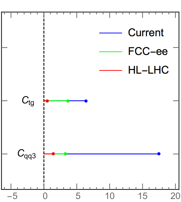
Finally, we study as well projected errors for a potential future FCC-ee machine. Details of this project are provided in [56], where it is indicated that the top-quark width can be probed with a precision of 45 MeV. We use this estimated error together with the more optimistic HL-LHC systematic error estimate to check what bounds the total width can provide on several example operators for each machine. The 68% CL uncertainties for the current measurement and the future colliders for and are shown in Fig. 7, where the blue, green, and red bars correspond to the uncertainties from the current measurement, FCC-ee, and HL-LHC (), respectively. We find that the bounds are significantly improved at both future colliders.
6 Conclusions
In this manuscript we have studied the next-to-leading order corrections to top quark decays within the SMEFT. Our calculation includes a more complete set of operators than previously studied, in particularly all contributing four-Fermi operators. We have two primary motivations. First, this work is a step toward a complete calculation of NLO effects within SMEFT, which we believe will eventually be required by the experimental uncertainties. Second, this work tests the question of whether loop-induced operators can be probed with either current or potential future collider data.
We have addressed technical aspects associated with higher-order calculations in the SMEFT containing . Chiral Ward identities play an important role in imposing consistency of prescriptions at higher-order in dimensional regularization, which we demonstrate by checking the consistency of several different schemes at one-loop order. Finally, we have presented numerical bounds on the considered operators given current and projected future uncertainties. We find that future machines such as the HL-LHC or a future collider can provide important constraints on SMEFT operators that first appear at higher-orders.
Acknowledgments
We thank C. Zhang for useful discussions. R. B. is supported by the DOE contract DE-AC02-06CH11357. C.-Y. C. is supported by the NSF grant NSF-1740142. F. P. and D. W. are supported by the DOE grants DE-FG02-91ER40684 and DE-AC02-06CH11357. This research used resources of the Argonne Leadership Computing Facility, which is a DOE Office of Science User Facility supported under Contract DE-AC02-06CH11357.
Appendix A NLO expressions for the helicity fractions
We present here the analytic results for the NLO SMEFT corrected helicity fractions and the total decay width of . For convenience we split up the different contributions.
| (34) |
where the first term in the expansion describes the contributions coming from the tree-level diagrams only (with full dependence retained), while the second one contains all QCD-like corrections expanded up to order and the last the pieces from the four-Fermi operators. We consistently expanded all three contributions to leading order in .
A.1 QCD corrected decay fractions
| (35) |
| (36) |
| (37) |
A.2 Four-fermion corrected decay fractions
Here we report the four-Fermi corrected longitudinal and negative transverse helicity fractions, and the total decay width of . We omit the contributions stemming from the vertex leading to two massless quarks in the loop.
| (38) |
| (39) |
| (40) |
References
- [1] W. Buchmuller and D. Wyler, Nucl. Phys. B 268, 621 (1986). doi:10.1016/0550-3213(86)90262-2
- [2] B. Grzadkowski, M. Iskrzynski, M. Misiak and J. Rosiek, JHEP 1010, 085 (2010) doi:10.1007/JHEP10(2010)085 [arXiv:1008.4884 [hep-ph]].
- [3] Z. Han and W. Skiba, Phys. Rev. D 71, 075009 (2005) doi:10.1103/PhysRevD.71.075009 [hep-ph/0412166].
- [4] A. Pomarol and F. Riva, JHEP 1401, 151 (2014) doi:10.1007/JHEP01(2014)151 [arXiv:1308.2803 [hep-ph]].
- [5] C. Y. Chen, S. Dawson and C. Zhang, Phys. Rev. D 89, no. 1, 015016 (2014) doi:10.1103/PhysRevD.89.015016 [arXiv:1311.3107 [hep-ph]].
- [6] J. Ellis, V. Sanz and T. You, JHEP 1407, 036 (2014) doi:10.1007/JHEP07(2014)036 [arXiv:1404.3667 [hep-ph]].
- [7] J. D. Wells and Z. Zhang, Phys. Rev. D 90, no. 3, 033006 (2014) doi:10.1103/PhysRevD.90.033006 [arXiv:1406.6070 [hep-ph]].
- [8] A. Falkowski and F. Riva, JHEP 1502, 039 (2015) doi:10.1007/JHEP02(2015)039 [arXiv:1411.0669 [hep-ph]].
- [9] J. de Blas, M. Ciuchini, E. Franco, S. Mishima, M. Pierini, L. Reina and L. Silvestrini, JHEP 1612, 135 (2016) doi:10.1007/JHEP12(2016)135 [arXiv:1608.01509 [hep-ph]].
- [10] C. Hartmann and M. Trott, JHEP 1507, 151 (2015) doi:10.1007/JHEP07(2015)151 [arXiv:1505.02646 [hep-ph]].
- [11] C. Hartmann and M. Trott, Phys. Rev. Lett. 115, no. 19, 191801 (2015) doi:10.1103/PhysRevLett.115.191801 [arXiv:1507.03568 [hep-ph]].
- [12] A. Dedes, M. Paraskevas, J. Rosiek, K. Suxho and L. Trifyllis, JHEP 1808, 103 (2018) doi:10.1007/JHEP08(2018)103 [arXiv:1805.00302 [hep-ph]].
- [13] R. Gauld, B. D. Pecjak and D. J. Scott, JHEP 1605, 080 (2016) doi:10.1007/JHEP05(2016)080 [arXiv:1512.02508 [hep-ph]].
- [14] R. Gauld, B. D. Pecjak and D. J. Scott, Phys. Rev. D 94, no. 7, 074045 (2016) doi:10.1103/PhysRevD.94.074045 [arXiv:1607.06354 [hep-ph]].
- [15] S. Dawson and P. P. Giardino, Phys. Rev. D 97, no. 9, 093003 (2018) doi:10.1103/PhysRevD.97.093003 [arXiv:1801.01136 [hep-ph]].
- [16] S. Dawson and P. P. Giardino, Phys. Rev. D 98, no. 9, 095005 (2018) doi:10.1103/PhysRevD.98.095005 [arXiv:1807.11504 [hep-ph]].
- [17] C. Hartmann, W. Shepherd and M. Trott, JHEP 1703, 060 (2017) doi:10.1007/JHEP03(2017)060 [arXiv:1611.09879 [hep-ph]].
- [18] S. Dawson and A. Ismail, Phys. Rev. D 98, no. 9, 093003 (2018) doi:10.1103/PhysRevD.98.093003 [arXiv:1808.05948 [hep-ph]].
- [19] S. Dawson, P. P. Giardino and A. Ismail, arXiv:1811.12260 [hep-ph].
- [20] C. Degrande, J. M. Gerard, C. Grojean, F. Maltoni and G. Servant, JHEP 1207, 036 (2012) Erratum: [JHEP 1303, 032 (2013)] doi:10.1007/JHEP07(2012)036, 10.1007/JHEP03(2013)032 [arXiv:1205.1065 [hep-ph]].
- [21] E. Vryonidou and C. Zhang, JHEP 1808, 036 (2018) doi:10.1007/JHEP08(2018)036 [arXiv:1804.09766 [hep-ph]].
- [22] L. Berthier and M. Trott, JHEP 1505, 024 (2015) doi:10.1007/JHEP05(2015)024 [arXiv:1502.02570 [hep-ph]].
- [23] G. Passarino and M. Trott, arXiv:1610.08356 [hep-ph].
- [24] N. Greiner, S. Willenbrock and C. Zhang, Phys. Lett. B 704, 218 (2011) doi:10.1016/j.physletb.2011.09.026 [arXiv:1104.3122 [hep-ph]].
- [25] C. Zhang, N. Greiner and S. Willenbrock, Phys. Rev. D 86, 014024 (2012) doi:10.1103/PhysRevD.86.014024 [arXiv:1201.6670 [hep-ph]].
- [26] A. Buckley, C. Englert, J. Ferrando, D. J. Miller, L. Moore, M. Russell and C. D. White, JHEP 1604, 015 (2016) doi:10.1007/JHEP04(2016)015 [arXiv:1512.03360 [hep-ph]].
- [27] V. Cirigliano, W. Dekens, J. de Vries and E. Mereghetti, Phys. Rev. D 94, no. 3, 034031 (2016) doi:10.1103/PhysRevD.94.034031 [arXiv:1605.04311 [hep-ph]].
- [28] J. A. Aguilar-Saavedra et al., arXiv:1802.07237 [hep-ph].
- [29] N. P. Hartland, F. Maltoni, E. R. Nocera, J. Rojo, E. Slade, E. Vryonidou and C. Zhang, arXiv:1901.05965 [hep-ph].
- [30] C. Zhang, Phys. Rev. D 90, no. 1, 014008 (2014) doi:10.1103/PhysRevD.90.014008 [arXiv:1404.1264 [hep-ph]].
- [31] P. Azzi et al. [HL-LHC Collaboration and HE-LHC Working Group], arXiv:1902.04070 [hep-ph].
- [32] A. Dedes, W. Materkowska, M. Paraskevas, J. Rosiek and K. Suxho, JHEP 1706, 143 (2017) doi:10.1007/JHEP06(2017)143 [arXiv:1704.03888 [hep-ph]].
- [33] E. E. Jenkins, A. V. Manohar and M. Trott, JHEP 1310, 087 (2013) doi:10.1007/JHEP10(2013)087 [arXiv:1308.2627 [hep-ph]].
- [34] E. E. Jenkins, A. V. Manohar and M. Trott, JHEP 1401, 035 (2014) doi:10.1007/JHEP01(2014)035 [arXiv:1310.4838 [hep-ph]].
- [35] R. Alonso, E. E. Jenkins, A. V. Manohar and M. Trott, JHEP 1404, 159 (2014) doi:10.1007/JHEP04(2014)159 [arXiv:1312.2014 [hep-ph]].
- [36] M. Fischer, S. Groote, J. G. Korner and M. C. Mauser, Phys. Rev. D 63, 031501 (2001) doi:10.1103/PhysRevD.63.031501 [hep-ph/0011075].
- [37] H. S. Do, S. Groote, J. G. Korner and M. C. Mauser, Phys. Rev. D 67, 091501 (2003) doi:10.1103/PhysRevD.67.091501 [hep-ph/0209185].
- [38] K. G. Chetyrkin and F. V. Tkachov, Nucl. Phys. B 192, 159 (1981). doi:10.1016/0550-3213(81)90199-1
- [39] F. Jegerlehner, Eur. Phys. J. C 18, 673 (2001) doi:10.1007/s100520100573 [hep-th/0005255].
- [40] T. L. Trueman, Z. Phys. C 69, 525 (1996) doi:10.1007/BF02907437 [hep-ph/9504315].
- [41] S. A. Larin, Phys. Lett. B 303, 113 (1993) doi:10.1016/0370-2693(93)90053-K [hep-ph/9302240].
- [42] P. Breitenlohner and D. Maison, Commun. Math. Phys. 52, 39 (1977). doi:10.1007/BF01609070
- [43] D. J. Broadhurst and A. G. Grozin, Phys. Rev. D 52, 4082 (1995) doi:10.1103/PhysRevD.52.4082 [hep-ph/9410240].
- [44] J. F. Donoghue, E. Golowich and B. R. Holstein, Camb. Monogr. Part. Phys. Nucl. Phys. Cosmol. 2, 1 (1992) [Camb. Monogr. Part. Phys. Nucl. Phys. Cosmol. 35 (2014)], Section III-3.
- [45] V. Shtabovenko, J. Phys. Conf. Ser. 762, no. 1, 012064 (2016) doi:10.1088/1742-6596/762/1/012064 [arXiv:1604.06709 [hep-ph]].
- [46] M. Jamin and M. E. Lautenbacher, Comput. Phys. Commun. 74, 265 (1993). doi:10.1016/0010-4655(93)90097-V
- [47]
A. V. Bednyakov, A. F. Pikelner and V. N. Velizhanin,
J. Phys. Conf. Ser. 523, 012045 (2014)
doi:10.1088/1742-6596/523/1/012045
[arXiv:1309.1643 [hep-ph]];
A. V. Bednyakov, A. F. Pikelner and V. N. Velizhanin, Phys. Lett. B 722, 336 (2013) doi:10.1016/j.physletb.2013.04.038 [arXiv:1212.6829 [hep-ph]];
D. Stöckinger, Dimensional regularization and , FCCee workshop talk (2018)” - [48] K. Adel and Y. P. Yao, Phys. Rev. D 53, 374 (1996) doi:10.1103/PhysRevD.53.374 [hep-ph/9408341].
- [49] S. Herrlich and U. Nierste, Nucl. Phys. B 455, 39 (1995) doi:10.1016/0550-3213(95)00474-7 [hep-ph/9412375].
- [50] W. E. Caswell, Phys. Rev. Lett. 33, 244 (1974).
- [51] M. Tanabashi et al. [Particle Data Group], Phys. Rev. D 98, no. 3, 030001 (2018). doi:10.1103/PhysRevD.98.030001
- [52] V. Khachatryan et al. [CMS Collaboration], Phys. Lett. B 762, 512 (2016) doi:10.1016/j.physletb.2016.10.007 [arXiv:1605.09047 [hep-ex]].
- [53] ATLAS Collaboration, ATL-PHYS-PUB-2019-005.
- [54] CMS Collaboration, CMS NOTE 2018-006.
- [55] C. Zhang and S. Willenbrock, Phys. Rev. D 83, 034006 (2011) doi:10.1103/PhysRevD.83.034006 [arXiv:1008.3869 [hep-ph]].
- [56] A. Abada et al. [FCC Collaboration], CERN-ACC-2018-0057.