Traffic Flow Characteristics and Lane Use Strategies for Connected and Automated Vehicle in Mixed Traffic Conditions
Abstract
Managed lanes, such as a dedicated lane for connected and automated vehicles (CAVs), can provide not only technological accommodation but also desired market incentives for road users to adopt CAVs in the near future. In this paper, we investigate traffic flow characteristics with two configurations of the managed lane across different market penetration rates and quantify the benefits from the perspectives of lane-level headway distribution, fuel consumption, communication density, and overall network performance. The results highlight the benefits of implementing managed lane strategies for CAVs: 1) a dedicated CAV lane significantly extends the stable region of the speed-flow diagram and yields a greater road capacity. As the result shows, the highest flow rate is 3,400 vehicles per hour per lane at 90% market penetration rate with one CAV lane; 2) the concentration of CAVs in one lane results in a narrower headway distribution (with smaller standard deviation) even with partial market penetration; 3) a dedicated CAV lane is also able to eliminate duel-bell-shape distribution that is caused by the heterogeneous traffic flow; and 4) a dedicated CAV lane creates a more consistent CAV density, which facilitates communication activity and decreases the probability of packet dropping.
top=1in,left=1in,bottom=1in,right=1in
1 Introduction
The mobility landscape is experiencing a paradigm shift due to rapid advancements of the information and vehicular technologies. Among them, the connected and automated vehicle (CAV) technologies have been contributing to the adoption of next-generation vehicles that are equipped with connectivity (i.e., connected vehicles) and/or automation (i.e. automated vehicles). In spite of CAV’s immense benefits and potentials in reshaping the mobility landscape, the adoption of CAVs by consumers is still uncertain Chan 2017, although some lower-level vehicle automation in the form of driver-assistance system has been commercially available.
The near-term deployment of CAVs is characterized by mixed traffic conditions, where human-driven vehicles (HVs) and CAVs constantly interact with each other. The potential benefits from CAVs may be offset by the interactions among different types of vehicles. For example, the short following time gap (e.g., 0.6 ) is only feasible when a CAV follows another CAV. To overcome such shortcoming in near-term CAV deployment, managed lane strategies, such as CAV dedicated lane, is one of the promising solutions in order to facilitate the formation of the CAV strings. Practically, managed lane strategies are freeway lanes that are set aside and operated under various fixed and/or real-time strategies in response to certain objectives, such as improving traffic operation fhw 2008. It is also anticipated that managed lane strategies incentivize the adoption of CAV, just as they did for encouraging car-pooling or low emission vehicles.
The goal of this study is to investigate the impact of different lane use strategies under mixed traffic conditions at vehicle trajectory- as well as lane-level. For clarity, we refer mixed traffic condition to the condition that CAVs and HVs operate on the same roadway network in the following discussions. The contributions of the paper include:
- 1.
the analysis of CAV-enhanced traffic flow characteristics at the lane- and vehicle-level,
- 2.
the investigation of traffic performance with gradual introduction of CAV platoons under difference managed lane strategies, and
- 3.
the implications of managed lane strategies from a dedicated short-range communication (DSRC) communication perspective.
The remainder of the paper is organized as follows. Related work regarding the research of CAVs in mixed traffic and managed lanes is reviewed in Section 2, followed by the evaluation methodology, including customized CAV module and defined scenarios, in Section 3. The simulation results are presented and discussed in Section 4. Lastly, findings and recommendations are discussed in Section 5.
2 Literature Review
There have been numerous studies on the implementation and evaluation of CAVs in various traffic settings. Aligning with our research topic, we focused our literature search on two key aspects of CAV studies: 1) CAV evaluation in mixed traffic conditions at network level and 2) managed lane strategies for CAV.
2.1 CAV Evaluation in Mixed Traffic Conditions
Three main approaches have been used to assess the benefits of CAVs: 1) analytical study, 2) simulation evaluation, and 3) field test with equipped vehicles. On-road testing provides the utmost degree of realism with equipped automated driving systems (ADS) and real-world traffic environment. However, the safety and efficiency issues for testing CAV on public roads have been the major concern, especially after several severe CAV-involved accidents in recent years. Due to safety, technological, and budgetary limitations, the scale of a CAV field test at current stage tends to be small (e.g., with a handful of CAVs). As a result, the conclusions from these small-scale field tests may not be reliably generalized to a traffic flow level. Furthermore, it was estimated by Kalra and Paddock 2016 that billions of kilometers of road test would be required to achieve the desired level of confidence in terms of safety of an ADS Kalra and Paddock 2016. Thus, analytical and simulation approaches serve as two primary methods for evaluating traffic flow impact of CAVs.
The majority of the analytical models is based on macroscopic traffic flow models and may experience difficulty in faithfully capturing the complex phenomena in transportation networks, such as lane drop. Smith et al. 2015 proposed an analytical framework for assessing the benefits of CAV operations Smith et al. 2015. The results indicated that CAVs improved network mobility performance, even with low MRP and no managed lane policies. Throughput without managed lanes increased by 4%, 10%, and 16% at the MPR of 10%, 20%, and 30%, respectively. It was also discovered that the managed lane policy facilitated homogeneous CAV traffic flow leading to more consistent and stable network outputs. An analytical model for determining the optimal managed lane strategy was proposed in Hussain et al. 2016, where the maximum system throughput in a mixed traffic condition could be calculated under the assumption of random vehicle distribution on a freeway facility. Three types of headways (i.e., conservative, neutral, and aggressive) were used in the model. Wang et al. 2017 proposed a second-order traffic flow model for mixed traffic streams with HVs and AVs. The authors found that the second-order model consistently outperformed the first-order one in terms of the accuracy of traffic density when the variability of the penetration rate increases Wang et al. 2017 .
At the corridor level, a capacity of 4,250 vphpl (vehicle per hour per lane) was observed in Van Arem et al. 2006 on a 6-km highway segment with uniformly distributed ramps under full market penetration of CAVs. The study by Shladover et al. 2012 observed a pipeline capacity of 3,600 at 90% MPR of CAVs Shladover et al. 2012, where the pipeline capacity refers to the throughput observed on a single-lane roadway without any interference of lateral movements Hall and Tsao 1997. Arnaout and Arnaout 2014 evaluated CAVs under moderate, saturated, and over-saturated demand levels on a hypothetical 4-lane highway under different market penetrations. They found that 9,400 vehicles could be served within an hour when the CAV MPR reached 40% Arnaout and Arnaout 2014. Songchitruksa et al. 2016 assessed the network performance with CAVs on the 26-mile I-30 freeway in Dallas, TX and found the highest throughput being 4,400 vph at 50% MPR Songchitruksa et al. 2016 among four MPR scenarios (i.e., 10%, 30%, 50%, and 70%). Another study Lee et al. 2014 also revealed that the mobility benefits of CAV emerged at 30% MPR.
Liu et al. 2020 investigated the benefits of alleviating freeway merge bottleneck and compared the performance of CACC with ACC under full market penetration. The results showed that CACC yielded a 50% reduction in fuel consumption (as estimated with the EPA MOVES model) while increasing corridor capacity by 49%, compared to the ACC scenario Liu et al. 2020. With a subsequent test on an 18-km segment of SR-99, the research team found that deploying vehicle awareness device (VAD)-equipped vehicles along with managed lane strategies was helpful in improving corridor-level traffic flow under low and medium CAV market penetrations Liu et al. 2018. Besides MOVES, comprehensive modal emission model (CMEM) An et al. 1997, VT-Micro Rakha et al. 2004, the Future Automotive Systems Technology Simulator (FASTSim)Brooker et al. 2015 are among the commonly used vehicle emission models in quantifying potential environmental impact of deploying CAVs.
The potential impact of the short following time headway of CAVs on HVs has also been studied in previous studies. Among them, the KONVOI project found that the carry-over effect for CACC drivers in manual driving after the disengagement of the CACC system Casey and Lund 1992. In recent years, driving simulator has been employed to study the behavioral adaptation of human drivers operating in the vicinity of CAVs. Nowakowski et al. 2011 found that test participants are likely to drive under a shorter following distance in the presence of CACC platoons in the adjacent lane Nowakowski et al. 2011. A similar study was conducted by Gouy et al. 2014 to investigate the behavioral adaptation of human drivers along a CACC platoon, in which two CACC platoon configurations were tested: 1) a 10-truck platoon with 0.3-s intra-platoon headway and 2) a 3-truck platoon with 1.4-s intra-platoon headway. It was found that a smaller average HV headway was observed in the first scenario, under which participants spent more time under a 1-s headway. Although such short headway was generally deemed unsafe in previous studies (e.g., Fairclough et al. 1997).
2.2 CAVs and Managed Lanes
Managed lanes have been in practice over the years to improve target operation objectives, such as 1) promoting the adaptation of environmentally-friendly vehicles by offering priority usage to specific travel lanes (e.g., the California Clean Air Vehicle Decal Shewmake and Jarvis 2014), 2) encouraging car-pooling by adopting high-occupancy vehicle (HOV) lanes Chang et al. 2008, and 3) performing active traffic management with the aid of high-occupancy toll (HOT) lanes Gomez-Ibanez et al. 2018. a CAV lane is one variant of managed lane strategies that provides exclusive lane use privilege to CAVs. Although managed lane strategies have been widely applied to highway operation with successful cases, due to distinctive operational characteristics of CAVs, knowledge learned from a conventional managed lane may not be directly transferable to the implementation of a CAV lane.
The provision of a CAV-managed lane has two primary reasons. First, CAV-managed lanes can incentivize the adaptation of CAVs by offering priority usage to managed lanes, which typically provides better and more reliable travel because of active traffic management. More importantly and unique to CAVs, CAV-managed lanes can provide accommodations for the underlying operational characteristics of CAVs. A CAV is able to operate at a much closer headway than a human driver with the assistance of V2V wireless communication and the automated driving system (ADS) Nowakowski et al. 2011, Shladover et al. 2018. Hence, the necessary condition for realizing such a short following headway is the availability of the vehicle driving information of at least one of the predecessors on the same lane, i.e., through a CAV following another CAV. Otherwise, the string stability of CAVs cannot be guaranteed Swaroop et al. 1994, and the lack of thereof is termed as CAV degradation Wang et al. 2019, which could potentially be a major hurdle for CAVs operating in mixed traffic. A numerical example by Wang et al. 2019 has showed that the current technological maturity of CACC contributed negatively to the stability of heterogeneous flow Wang et al. 2019.
To mitigate CAV degradation, ad hoc coordination, local coordination, and global coordination are the three major strategies that outline the organization of CAV platoons Shladover et al. 2015. Ad hoc coordination assumes that CAVs arrive in random sequence and do not actively seek clustering opportunities in a traffic stream. By extension, the probability of driving around other CAVs is highly correlated to MPR. On the contrary, CAVs actively identify and approach an existing CAV cluster (or other free-agent CAVs) to form a new cluster through local coordination, regardless of CAV MPRs. Finally, global coordination (a.k.a. end-to-end platooning) requires a high-level route planning and extensive communication to coordinate vehicles traveling with the same origin-destination pair even before the CAVs entering highway sections Larson et al. 2013.
To successfully form and maintain platoons, accurate and cost-effective localization of CAVs in a dynamic traffic environment remains one of the biggest challenges, especially for local coordination Shladover et al. 2015, Kuutti et al. 2018. In the presence of a CAV-managed lane, a higher concentration of CAVs facilitates local coordination with much less stringent requirements on the accuracy of vehicle localization. In addition, the CAV-managed lane strategy aligns well with the three-stage deployment roadmap considering market diffusion and technological maturation for CAVs Zhong 2018. In the first stage, the adoption of CAVs is incentivized by allowing the use of the managed lane free of charge. At this stage, the following headway of CAVs on the managed lane may be comparable to that has been observed from HVs for safety reasons in a mixed traffic condition. In the second stage, a shorter following headway for CAVs could be implemented to further increase the carrying capacity of the managed lane when the demand of CAVs along with the familiarity of road users to CAVs increases. In the third stage, when the CAVs reach a critical level of MPR, high-performance driving enabled by the CAVs can be achieved due to homogeneous CAV traffic flow on the managed lane.
To assess the impact of CAV-managed lane strategies, Zhang et al. 2018 compared the performance of a managed lane and general propose lanes (GPL) based on average speed, throughput, and travel time Zhang et al. 2018. The results indicated that the speed improvement in the managed lane was significant compared to that of GPLs. With 20% MPR, the latent demand (the demand that cannot enter the simulation network due to congestion) decreased to zero. Inspired by the fluid approximation of traffic, Wright et al. 2018 proposed an algorithm for simulating the weaving activity at the interface of a managed lane and the adjacent GPL at a macroscopic scale Wright et al. 2018. Chen et al. 2016 proposed a time-dependent deployment framework that was formulated with a network equilibrium model and a diffusion model. With the constraint of a given set of candidate lanes which corresponds to the field condition, the social cost was minimized with the consideration of different MPR levels Chen et al. 2016. Zhong and Lee 2019 studied four managed lane strategies and compared the benefits for GPL and managed lane users in terms of mobility, safety, emission, and equity Zhong and Lee 2019. In freeway settings, the authors recommended a 30% minimal MRP for deploying a CAV-managed lane to avoid lane use imbalance that could degrade the performance Zhong 2018, Zhong and Lee 2018.
Qom et al. 2016 proposed a multi-resolution framework to study the mobility impact of CAV lanes. Traffic flow-based static traffic assignment and the meso-scopic simulation-based dynamic traffic assignment were adapted in the bi-level framework. The former yielded the MPR-based trends, whereas the latter refined the trend based on traffic congestion. The results indicated that it was not beneficial to provide toll incentive for CAVs at lower MPR due to the marginal increase in highway capacity Qom et al. 2016. Ghiasi et al. 2017 proposed an analytical capacity model for mixed traffic Ghiasi et al. 2017. The model relied on the Markov chain representation of the spatial distribution of heterogeneous and stochastic headway. With the sufficient and necessary condition of capacity increase proven, the authors emphasized the importance of quantitative analysis of the actual headway stetting.
The introduction of a CAV lane to a signalized corridor was reported in Zhong et al. 2017. Two configurations of a CAV lane, along with other managed lanes, were evaluated. Due to the turning nature of an arterial, buffer zones were implemented where HVs are allowed to temporarily use the CAV lane for turning movements. Papadoulis et al. 2019 evaluated the safety impact of CAVs using the Surrogate Safety Assessment Model (SSAM) Papadoulis et al. 2019. The time to collision (TTC) and the post encroachment time (PET) were adapted with safety thresholds of 1.5 s and 5 s, respectively. They observed substantial safety benefits in terms of reduction in traffic conflicts: 12-47% at 25% MPR to 90-94 % at 100% MPR. In Zhong et al. 2020, TTC was also used to assess the safety conditions for HVs when CAV local clustering strategy was employed. Ali et al. 2018 found that drivers with advanced traffic information enabled by connectivity tend to wait longer and maintained a larger space on mandatory lane change (the communication delay for lane merging assistance was unnoticeable when it was less than 1.5 s). Post-encroachment time (PET) analysis also indicated improved travel safety from CAV implementation Ali et al. 2018.
2.3 Summary
The vast majority of previous studies evaluated the benefits of CAVs at an aggregated level with the emphasis of overall traffic improvement. Analytic models are in macroscopic nature under overly ideal conditions, and they have difficulty in factoring in the stochastic nature of human drivers in a mixed traffic environment. CAV-managed lane strategy could be instrumental in the near-term deployment of CAVs, but it is still an under-explored area, despite its increasing recognition.
3 Evaluation Framework and Experiment Design
This study focuses on analyzing mixed traffic flow characteristics at a corridor level considering different CAV MRPs and managed lane strategies. In this section, the integrated simulation test bed, transportation network, and simulation scenarios are discussed in detail.
3.1 CAV Behavior Model
The PTV Vissim PTV AG 2018, a commercial-off-the-shelf microscopic simulation package, is chosen for the evaluation. Vissim has been widely adapted by transportation practitioners and researchers, owing to its high-fidelity simulation mechanism and flexible modules. Although compared to other open-source traffic simulators (e.g., SUMO), one reservation for Vissim being a commercial software is its close-sourced nature. As shown in Table 1, a calibrated Wiedemann car-following model and the Enhanced Intelligent Driver Model (E-IDM) Kesting et al. 2010 were used to model HVs and CAVs, respectively. The intelligent driver model (IDM) and its variants have been used to design the ACC/CACC controller that resembles human-like car-following behaviors Wang et al. 2019, Kesting et al. 2008, Talebpour et al. 2016, Spiliopoulou et al. 2017, Guériau et al. 2016. As an improved iteration of the collision-free IDM Treiber et al. 2000, the E-IDM deals with CAV longitudinal maneuver. The behavior model of the E-IDM is expressed in Eq. 1, 2, and 3.
| Vehicle Type | Longitudinal Control | DTG | Stochasticity |
| HV | Weidemann 99 | 1.4 s | Y |
| CAV | E-IDM | 0.6, 1.2 s | N |
| (1) |
| (2) |
| (3) |
where, is the maximum acceleration; is the desired deceleration; is the coolness factor; is the free acceleration exponent; is the current speed of the subject vehicle; is the desired speed, is the speed of the lead vehicle; is the minimal distance; is the acceleration of the subject vehicle; is the acceleration of the lead vehicle; is the acceleration calculated by the original IDM model Treiber et al. 2000. The minimal distance can be calculated as where is the desired time gap; and is the acceleration calculated by the constant-acceleration heuristic (CAH) component, where is the Heaviside step function that is used to eliminate the negative approaching rate of subject vehicle Kesting et al. 2010.
In this study, the E-IDM model is selected as the longitudinal control for the CAVs. Although without built-in multi-anticipative car-following function, as the literature shows, E-IDM is still a good simple car-following model for CAVs, as the stochastic nature of human driving is removed (i.e., automation property), and the acceleration of the preceding vehicle is taken into account in the driving model (i.e., connectivity property). As shown in Table 2, all the parameters remain the same as those originally specified in Kesting et al. 2010, with the exception of the desired time gap (DTG), which is defined with two values: 0.6 s and 1.2 s. The former DTG is used when the communication between a preceding CAV and the subject CAV is successful, whereas the latter one is in effect when the communication failure occurs. The updating frequency for the E-IDM model in Vissim is 10 Hz. The density of CAVs which is used to calculate the communication activity is updated at a 2-Hz frequency to reflect the traffic dynamic. Each transmission is assumed to have up to five attempts (four re-transmission). At least one successful attempt is required for a transmission to be considered successful, upon which the DTG is determined.
| Parameter | ||||||||
| value | 0.6 s | 1.2 s | 1 | 2 | 2 | 0.99 | 4 | 105 |
To implement these two car following models in Vissim, the subset of the human driving behavior is realized by adjusting car-following parameters of the Wiedemann car-following model, which is relatively straightforward. The E-IDM, on the other hand, is implemented via the external driver model application programming interface (API) and connected with Vissim through a dynamic link library (DLL). The DLL is invoked in each simulation time step such that the default car-following behavior will be overwritten for a specified vehicle type. The DSRC wireless communication module, discussed later in Section 3.2, is also implemented in the API to achieve a dynamic response based on prevailing traffic conditions.
One of the most prominent features in CAV behavior modeling is the short time headway during car-following, which is manifested by several key differences between a CAV and a HV. First, the stochasticity of the CAVs is significantly lower than that of human drivers. This is enabled by the on-board sensors that are able to continuously and accurately perceive the surrounding environment. However, the stochaticity cannot be completely eliminated due to sensor noise and communication delay/error. Second, a CAV has minimal reaction time due to its algorithmic decision making process and computational power. Past studies have already identified that the impact of the reaction time of human drivers in various traffic phenomena, including capacity drop Calvert et al. 2018 and flow stability Talebpour et al. 2016, whereas driving simulation tests revealed that the information augmented by connectivity could decrease the reaction time for drivers [Sharma et al. 2019].
In addition, human factor plays a crucial role in the resumption of control of a CAV when an ADS exits its operational domain (e.g., high risk of collision, sensor failure, communication interference). Quantitative evidence regarding the transition of control from traffic psychology or human-machine interactions is still limited Calvert and van Arem 2020, though few frameworks have been proposed to simulate human behavior endogenously van Lint and Calvert 2018, Saifuzzaman et al. 2017. For example, the prospect theory was used to model the risk and human perception Hamdar et al. 2015, Sharma et al. 2019. The Risk Allostasis Theory Fuller 2011 was adopted for modeling relationship between cognitive processing of information and physical performance. The Task Capacity Interface Saifuzzaman et al. 2015 was employed by Saifuzzaman et al. 2015 for quantifying situational awareness of a driver.
Calvert and van Arem 2020 developed a framework that encompasses the driving task demand and driver task saturation Calvert and van Arem 2020. The framework’s main goal is to assess the performance impact during the transition of control for AVs. The total task demand, situational awareness, and reaction time during the transition of control from AVs was explored. The framework showed promising capability in capturing the interactive effects of humans with lower level AVs. However, empirical evidence is still needed to relax the assumptions used in the framework from not only the cognitive point of view, but also from vehicle dynamics and inter-vehicle interactions.
Another human factor is driver compliance to the ADS. Since in lower or medium level of automation, the driver is ultimately responsible for his or her vehicle, which means overwriting, when deemed necessary, is possible by the human driver. This control authority, in extreme cases, could cancel out the benefits promised by the CAV technologies. In a recent study [Sharma et al. 2019], Sharma et al. 2019 employed the prospect theory to model driver decision-making mechanisms including irrational ones, and captured the negative relationship between headway and compliance decision by a driver.
In this study, we represent the differences of a CAV and a HV with different desired time headways through separate car following models, with the following assumptions made for CAVs: 1) no error for the on-board sensors and the vehicle controller, i.e., perfect perception; 2) no human factor modeling pertaining to the transition of authority; and 3) no behavior adaptation for CAVs for non-CAV drivers.
3.2 Wireless Communication Model
In an early study, we implemented a packet-level communication module through Vissim API Zhong and Lee 2018. Similar adaptations for the model were also found in previous studies Songchitruksa et al. 2016, Zhong and Lee 2018, Bibeka et al. 2019. The analytical model Killat et al. 2007 was developed from ns-2, an empirical packet-level network simulator that returns the probability of one-hop broadcast reception of basic safety message (BSM) under IEEE 802.11p, an approved amendment tailored to wireless access in vehicular environment (WAVE) in the 802.11 family protocol. The model uses the concept of communication density level, a metric representing channel load in vehicular communication in the form of the sensible transmission per unit of time and per unit of the road Jiang et al. 2007. The data reception rate is determined jointly by communication density level and transmission power. An illustration for the reception probability is shown in B. Note that this communication model only pertains to the physical layer of the DSRC communication (e.g., no MAC layer delay).
| (4) | ||||
where, is the two-dimensional polynomial of fourth-degree for all curving fitting parameters Killat and Hartenstein 2009, which is also shown in B; is communication density, events/s/km; and is the transmission power, m; is vehicle per kilometer that periodically broadcast messages, veh/km; and is transmission rate, Hz.
3.3 Transportation Network
A 9.3-km 4-lane hypothetical network was constructed in Vissim with two interchanges located at mile marker 2 (km) and 6 (km) respectively. An abstract geometry of the network along with vehicle demand of the origins and destination is shown in Figure 1. The primary reason for using a simply synthetic network is to limit variables for the simulation. Note that the driving behavior parameters for the Wiedemann car-following model (for HVs) is the same as in previous studies Leidos 2016, Li et al. 2019, Zhong 2018, Zhong et al. 2020, which represents a subset of the calibrated driving behavior in the I-66 segment in northern Virginia. The demand originated on the mainline is deliberately set higher than usual to create a congested network. The speed limit for the mainline of the network is set as 120 . Three data collectors are placed at “C1”, “C2”, and “C3” locations.

3.4 Managed Lane Scenarios
Three cases of CAV lanes, as shown in Table 3, are implemented in the network:
- •
No managed lane (NML): This scenario serves as the base condition of the study. There is no priority lane use for CAVs, and they are mixed with HVs throughout the network;
- •
One CAV lane (CAV-1): In this strategy, one CAV lane is implemented in the left-most lane (the fourth lane from the right);
- •
Two CAV lanes (CAV-2): An additional CAV lane is added to the CAV-1 case, making two CAV lanes available at the leftmost and the second leftmost lane in the roadway segment. It aims to investigate the duel managed lane configuration.
As revealed in previous studies Zhong 2018, Zhang et al. 2018, Xiao et al. 2019, Transportation Research Board 2018, a managed lane may have a detrimental effect on traffic performance if implemented prematurely, i.e., usually with an MPR less than 30%. Therefore in this study, we set CAV MPRs for “CAV-1” to start from 30%. With the same logic, the “CAV-2” cases start with 40% to cover certain transition MPR, since the linear extrapolation may not hold.
| Policy | No Managed Lane | Managed Lane #1 | Managed Lane #2 |
| ID | NML | CAV-1 | CAV-2 |
| 1st Lane | HV + CAV | HV + CAV | HV + CAV |
| 2nd Lane | HV + CAV | HV + CAV | HV + CAV |
| 3rd Lane | HV + CAV | HV + CAV | CAV |
| 4th Lane | HV + CAV | CAV | CAV |
| MPR | 0% - 100% | 30% - 100% | 40% - 100% |
4 Results and Analysis
Five replications are run for each combination of managed lane policies and MPRs. Aggregated data are collected at 5-min intervals, and the raw data are collected at each simulation time step. The analysis is performed on four aspects: 1) traffic flow characteristics, 2) headway distribution, 3) fuel consumption, 4) wireless communication, and 5) overall network performance.
4.1 Traffic Flow Characteristic
Figure 2 exhibits the speed-flow characteristics of the simulation scenarios having 40% MPR and above. The plot is color-coded by travel lanes with index “1” representing the rightmost lane, and “4” the leftmost. The speed-flow diagram is comprised of a stable region and a unstable (congested) region, separated by the optimum (maximum) flow. Several distinctive patterns can be observed. First, regardless of the managed lane strategy, the sample points become more concentrated as the MPR increases, with the disappearance of the congested region typically found in the lower speed region. Second, the CAV lane has a distinct pattern compared to the GPLs. Such pattern is most apparent in CAV-1, where the traffic samples on the leftmost lane (CAV lane) shift to the right along the flow axis. The congested region disappears when MPR reaches 70% in the CAV-1 case for all of the lanes. The improvement for the GPs is due to a higher carrying capacity of the CAV lane, which results in less traffic on the GPLs. The homogeneity of the CAV traffic is the primary factor in realizing the mobility benefit of CAVs: in NML cases, the sample points from difference lanes are evenly distributed, in contrast to managed lane cases. For the CAV-2 case, the separation of the CAV lanes (leftmost and the second leftmost) started to show at 70% MPR. At full penetration (100%), the traffic patterns are very similar, as the managed lane becomes irrelevant.
4.2 Headway Distribution
The simulation collects raw data from the data collector, an equivalent of real-world detectors (e.g., loop detectors, video cameras, microwave sensors). By analyzing the high-resolution raw data (collected every 0.1 s), the headway distribution in CAV lanes can be obtained. Recall that the collectors are placed in three sections of the roadway segment, as shown in Figure 1.
The cumulative probability function (CDF) curves are displayed in Figure 3. The vertical lines in the figure are the headways when 100% cumulative probability is reached. The slope of the CDF indicates the level of concentration of the samples within a distribution. In NML cases, two types of tipping points exist: the one at lower headway resulted from a high MPR and the one with higher headway observed at a low MPR (below 40%). For CAV-1, the pattern for CDF at 30% and 40% is transformed to the pattern observed at high MPRs. With 2 CAV lanes, the CDF increases gradually in the mid-range MPR (40% to 60%) because of under-saturation on the CAV lanes, as illustrated in the CDF on the 3rd and 4th lanes. Such under-saturation situation is alleviated when the MPR reaches 70%. A similar pattern in CDFs is observed at a high MPR range (i.e., 80% to 90%) regardless of the managed lane strategies, indicating a high concentration of samples with headway above 1 s.

Two-sample Kolmogorov-Smirnov (K-S) test is adopted to analyze the CDFs to check whether two random samples are from the same population Goodman 1954. It is a non-parametric test where no assumption is made regarding the distribution of the variables Young 1977. The null hypothesis () of the two-sample K-S test is that the two sample sets are from the same continuous distribution. Nearly all the CDFs in the pairwise comparison rejects the null hypothesis with a low p-value at the 0.05 significance level, with the exception of the comparison of 40% and 50% in NML. Figure 4 is a heatmap that shows the pairwise K-S statistic that represents the supremum of the two tested empirical CDFs. The denser the color, the higher the difference in cumulative probability between two comparing scenarios.
The average headway for HVs and CAVs in every travel lane is shown in Figure 5. The row represents the vehicle types, whereas the column represents the travel lane. Recall that the 4th lane is the leftmost lane. For HVs, their averaged headway decreases as the MPR increases in CAV-1 and CAV-2 cases. While the headway also decreases in the NML case, it is at a lesser rate. When it comes to CAVs, the decreasing rate in CAV-2 is greater than that in CAV-1 or NML. The mean headway is around 4 s in CAV-2 case when the MPR is low or in mid-range due to low lane utilization in the CAV lanes. The average headway in CAV-2 case reaches a comparable level to its counterparts at 70% MPR, which is the deflection point. The lowest mean headway achieved among all scenarios is observed at 70% MPR in CAV-1 case for CAVs, which corresponds to the maximum capacity with all other factors being equal. Lastly, the headway trend for CAVs remains a similar pattern across four travel lanes in the NML case, since CAVs are uniformly distributed across all lanes.
Figure 6 shows the comparison of headway distributions in the leftmost lane among three managed lane scenarios under different MPRs. In the 40% to 70% MPR range, it is shown that implementing a managed lane for CAVs clearly shifts the distribution to the left-hand side, which represents smaller headways. The distributions of headway collected for either CAV-1 or CAV-2 become “narrower” (with less standard deviation), as the MPR increases from 40% to 70%. The highest bin of the histogram for both CAV-1 and CAV-2 cases is 1 s - 1.2 s when the MPR is below 50%. When the MPR is higher than 50%, the highest bin of the histogram shifts to 0.8 s - 1 s. In comparison, the NML case does not exhibit such a concentration pattern as the MPR increases. The result indicates that a homogeneous traffic flow comprised of only CAVs is able to realize the short-headway benefits from deploying CAVs.


4.3 Fuel Consumption
The VT-Micro model Rakha et al. 2004, an individual vehicle and operation-level emission model, is adopted to calculate the instantaneous fuel consumption rate. The inputs for the VT-Micro model are instantaneous vehicle speed and acceleration, and the output is the second-by-second fuel consumption rate, as shown in Equation 5, where is the instantaneous speed, is instantaneous acceleration, and are regression coefficients for emission and fuel consumption at speed power and acceleration power , respectively.
| (5) |
The vehicle data was derived from the raw data from the detectors in three locations (marked in Figure 1). The result for the fuel consumption is plotted in Figure 7, which shows two distinctive patterns for the GPLs and the managed lane. The concentration of fuel consumption is within 5 to 10 for lanes that allows HV operation (i.e., mixed traffic), when the MPR for CAVs is equal or less than 60%. When the MPR rises to above 60%, the instantaneous fuel consumption shifts to a lower values with a “narrower” slope: higher concentration between 5 and 7 .

We then isolate the CDF curve for both CAVs and HVs, when they operate on the leftmost lane under homogeneous flow condition. More specifically, the separated CDF curves represent the observations of HVs from the 0% MPR in NML case and the observations for CAVs from the 100% MPR for CAV-1 case. The CDF curves in Figure 7 exhibit two different patterns for CAVs and HVs. The former with 60% of the observations fall below 4 , whereas the latter with 60% of the observations below 12 with a wider spread. The wider spread for HVs is probably caused by the stochastic nature of human drivers (which is simulated by the Wiedemann model). Hence the mixed traffic condition is comprised of two competing flows that excreting their influence.
In the GPLs, the MPR plays as an indicator for the dominance of each traffic flow. The higher the MPR, the closer the CDF curves approach the pattern of managed lane that is used by CAV exclusively. In the managed lane, the CAV traffic is the sole dominating traffic. Therefore, the fuel consumption curve exhibits only CAV traffic characteristics, regardless of the MPR. We include the fuel consumption rate CDF curves for HVs and CAVs in Appendix II (Figures 2 and 3) - both figures demonstrate the shift towards CAV fuel consumption CDF pattern as the MPR grows.


4.4 Wireless Communication
Figure 8(a) shows the maximum and the average density for instances of V2V communication among three managed lane policies. Recall the DSRC communication model only deals with the physical layer. While the transmission density increases as the MPR increases, the maximum density in NML is higher than CAV-1 and CAV-2, because the CAV platoons were broken down by certain HVs which are susceptible to shockwaves. As such, the traffic flow is compressed, producing a higher traffic density and thus higher transmission density. With the aid of CAV lane, the communication density is thus maintained at a lower level. In a CAV lane, the CAVs distribute longitudinally on the managed lane. The NML, in comparison with two managed lane cases, is more likely to generated pockets of traffic with CAVs across multiple lanes, which could result in localized higher transmission activity.
The probability of successful reception of BSM from a leading vehicle to a subject vehicle is shown in Figure 8(b). The probability curves under CAV-1 and CAV-2 scenarios are in close proximity to each other and they are showing the same trend. The maximum difference between these two curves is 0.04 at 90% MPR. The probability of successful communication of NML at high MPR range (60% to 90%) is consistently lower than those of CAV-1 and CAV-2. This is caused by the compression of traffic flow by localized shockwaves. There is an overall decreasing trend of the probability as the MPR increases, but still remains a successful rate of 94% and above.
4.5 Network Performance
The measures used in this section gauges the overall performance of the simulation network at an aggregated level. The throughput represents the total number of vehicles that have arrived at their destinations, shown in Figure 9. As mentioned before, the network was configured with a higher than usual demand. With a 10,000-vph demand for a four-lane highway, the network was only able to process 6,500 vph in the absence of CAVs. Under the NML scenario, as the MPR of CAVs increases, so does the network throughput. The throughput reaches approximately 8,000 vph with 40% and 50% MPRs. However, at 60% MPR, the network throughput is boosted again and maintains at the same level at 9,600 vph when the MPR is above 70%. The throughput in CAV-1 case begins to outperform the NML case at MPR 50% and keeps increasing to 9700 vph at 70% MPR, where the throughput starts leveling in spite of the increase in MPR. For the CAV-2 policy, the system throughput only reaches the same level of the two counterparts at 70% MPR due to under-utilization of CAV lanes with low MRPs.

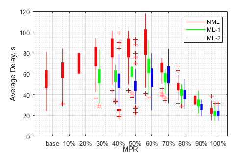

The average delay experienced by vehicles (plotted in Figure 1(a)) within the network is calculated by dividing the total delay by the sum of the vehicles within the network and the vehicles that have exited the network. For three strategies, the average delay starts to decrease as the throughput levels off: at 60% for NML and CAV-1, and at 70 % for CAV-2. Such seemingly counter-intuitive phenomena could be explained by taking into account the average speed, which is shown in Figure 1(b): when the throughput is in a graduate increase as the MPR goes until 60%, the average speed exhibits a decreasing trend, which is in an inverse relationship with vehicle delay. This trend is in agreement with the speed-flow fundamental diagram.
5 Discussion and Conclusions
In this section, we highlight the findings from the previous section and discuss the study in a boarder context.
5.1 Summary
The analysis results indicate that the introduction of CAV could increase the throughput of the overall system, even when no managed lane policy is in place. The congestion region in the speed-flow diagram disappears as the MPR of the CAVs increases. This is an indication of the improvement of roadway capacity owing to CAVs, which is consistent with the findings of previous studies. More importantly, the congestion region first disappears in the CAV lane in CAV-1 case, illustrating that the homogeneity of CAV traffic results in a more stable traffic flow with a high throughput. A CAV lane, with an MPR of as low as 40%, is able to accommodate more traffic compared to a GP lane and it helps to alleviate the overall congestion of the network. The average vehicle delay exhibits a decreasing trend, even after the network throughput levels after 70% MPR. This is an indicator that the network is able to carry additional traffic than the high demand specified in Fig. 1.
The individual headways among consecutive vehicles are measured for each lane. From the headway distribution, one can not only measure the compactness of the traffic but also the stability of the traffic flow. Both HVs and CAVs have a predominate headway as shown in Table 1. In a heterogeneous traffic flow, two spikes with different tipping points can be observed in the headway CDF curve. Each segments indicates a high concentration for the headway samples. One is for the following headway samples observed on HVs, and the other is for the headway samples for CAVs. With traffic homogeneity on the CAV lane, there is only one spike on the CDF curves. The magnitude of the spike also depends on the lane occupancy, as evidenced by the comparison of CAV-1 and CAV-2 at the same MPR. The two-spike pattern remains even at high-range MPR (i.e., 60-80%) in the absence of CAV lane (the NML case).
The VT-Micro model, which produces instantaneous fuel consumption for individual vehicles, was employed to estimate the environmental impact of the CAV lane. The vehicle speed and acceleration was collected as inputs and the relative fuel consumption, instead of the absolute one, is examined. Again, distinct patterns for a GPL and a CAV lane were observed. The average instantaneous fuel consumption for CAV lane has a narrower distribution.
Lastly, the DSRC communication was measured using an analytical communication model that is derived from a package-level network simulator. It simulates the physical layer of the DSRC communication that is an integral element of CAVs. We found a lower communication density in CAV lane, as the CAVs were more evenly distributed longitudinally. A lower communication density indicates a less congested communication channel, which increases the performance of the V2V communication. Compared to CAV-1 and CAV-2 scenarios, it is more likely under NML scenario to generate pockets of traffic with CAVs across multiple lanes, which could introduce higher localized transmission activity and increase the loss of BSM packets.
The overall results show that a single CAV lane in a four-lane highway network is able to provide the necessary technical accommodation efficiently in the mixed traffic conditions with a wide range of MPR. A CAV dedicated lane is helpful to guarantee the benefits of CAVs, as it creates a homogeneous CAV flow. Implementing two CAV lanes, however, may adversely affect the overall traffic, especially when the MPR of CAV does not warrant an additional CAV lane.
5.2 Limitations
While the paper demonstrates the benefits of managed lane for CAV at lane- and vehicle- levels, we should note that there are limitations in this study and the benefits are realized in a controlled environment under certain assumptions. First of all, although the Wiedemann model is behaviorally sound and has been adopted by numerous researchers for simulating human drivers, the complexity of a human drivers under dynamic traffic conditions is difficult, if possible at all, to be captured by simulation models. In addition, the behavioral adaption for human drivers in the presence of CAV is not known yet, due to the lack of empirical evidence in the public domain. Preliminary results revealed that a smaller time headway was adopted by a HV when driving along side with closed platooned CAVs Gouy et al. 2014. Note that the Wiedemann driver behavior parameters were calibrated using field data where CAVs have not been deployed on the roadway yet. The calibrated parameters represents a subset of the driving population, and they may not directly transferable to other driving conditions or demographics. The E-IDM, while being widely adopted, does not contain the multi-anticipative car-following feature, which has been promoted as one of the crucial feature enabled by V2V communication. Therefore, the performance of the CAVs are expected to be more conservative. Like many existing CAV car-following models, the E-IDM does not factor in the aspects of human factor that is anticipated to be more pronounced in the lower levels of automation.
In addition, there are several salient issues regarding the low level automation and its modeling as well. For a CAV, the drivers’ acceptance of short following headway (e.g., 0.6 s) is still an open question Nowakowski et al. 2011, given that the short following headway is technologically attainable. It is reasonable to expect that the acceptance of extremely short headway would be low initially, although it will gradually increase as CAV penetration increases. The pace of adaption, though, is largely depending of the level of confidence to the ADS from human drivers. The level of compliance from drivers (in the absence of automation) is also an important factor in harnessing rich information brought by the connectivity. The layer of driver stocatistcity in reacting to traffic information remains. In the extreme case, a complete disregard of useful information could negate the benefits of connectivity.
Another crucial issue is the transition of control from the ADS back to the human driver. As per the definition of vehicle automation by the SAE, the Level 3 automation (and below) requires a fallback receptive driver when the ADS exits its designed operational domain. As studies have shown, such fallback process is way more complicated than merely re-taking the steering wheel. First, a driver needs to regain situational awareness of the traffic environment from the disengagement of driving. The surge in cognitive demand during the initial period of re-engaging in driving tasks could result in deterioration in driver’s performance (e.g, increased reaction time, inadequate situational awareness). This aspect rarely exists in current CAV models, and much likely it will require an endogenous cognitive models that is able to take into account the driving task demand and the cognitive capacity of human drivers [Calvert and van Arem 2020]. Therefore, the human-machine interfacing is seldom captured in current simulation model, including the one used in this study.
5.3 Future Research
The future research would focus on relaxing the assumptions in this study. The first direction is the CAV behavior modeling. Researchers have recently started the incorporation of human factor aspect, such as an extension module in IDM to model driver’s responses to advanced traffic information [Sharma et al. 2019], an endogenous model of human cognitive for the transition of control [Calvert and van Arem 2020]. Such developments offer a great opportunity to introduce human factor in a mixed traffic flow in the future. Second, the inner most lane is generally assigned as the managed lane in current practices, which requires eligible users to merge to access the managed lane, and induces additional demand of lane changing. The access plan (e.g., ingress and egress points of the managed lane, eligibility) requires further study to minimize the negative impacts caused by induced weaving activity. A cost-benefit analysis may also be warranted for comparing managed lane strategies with other emerging technologies, such as vehicle awareness device (VAD), for the near-term deployment of CAV. Some researchers have started the exploration of right-most managed lane in U.S. [Li et al. 2020]. Lastly, the characteristics of mixed traffic flow that is anticipated in the near-term deployment of CAV needs further exploration. Especially, the impact of CAVs at individual trajectory level by analyzing high-resolution vehicle trajectory data desires further exploration.
Appendix A List of Abbreviations
| Abbreviation | Definition |
| ADAS | advanced driver-assistance systems |
| ADS | automated driving systems |
| ACC | adaptive cruise control |
| AV | automated vehicles |
| API | application programming interface |
| BSM | basic safety message |
| CV | connected vehicles |
| CAV | connected and automated vehicles |
| CACC | cooperative adaptive cruise control |
| CAH | constant-acceleration heuristic |
| CDF | cumulative probability function |
| CHEM | comprehensive modal emission model |
| DSRC | dedicated short-range communication |
| DLL | dynamic-link library |
| DTG | desired time gap |
| E-IDM | enhanced intelligent driver model |
| GPL | general purpose lane |
| HV | human-driven vehicle |
| HOV | high-occupancy vehicles |
| IEEE | Institute of Electrical and Electronics Engineers |
| MPR | market penetration rate |
| MOVES | motor vehicle emission simulator |
| PET | post encroachment time |
| SSAM | surrogate safety assessment model |
| SAE | Society of Automotive Engineers International |
| SUMO | simulation of urban mobility |
| TTC | time to collision |
| VAD | vehicle awareness device |
| WAVE | wireless ac¬cess in vehicular environment |
Appendix B Coefficients for Wireless Communication Model
The coefficients obtained from the polynomial function is shown in Table 1a. It is worth stressed that even seemingly negligible values, if omitted, could result deviation in the probability of reception from 8% to 100% Killat and Hartenstein 2009.
| (0,0) | (1,0) | (2,0) | (3,0) | (4,0) | |
| 0.0209865 | -9.66304-07 | -1.72786-11 | 5.09506-17 | -7.91921-23 | |
| 2.24743 | 7.84884-07 | 2.28533-10 | -5.89802-16 | 3.55262-22 | |
| 2.56426 | 2.82287-05 | -7.09939-10 | 1.34371-15 | -3.01956-22 | |
| 2.41146 | -9.3285905 | 6.77403-10 | -9.64188-16 | 3.69652-23 | |
| (3,1) | (2,1) | (2,2) | (1,1) | (1,2) | |
| 3.16577-20 | 2.13587-14 | -5.05716-17 | 4.00928-09 | -1.88707-11 | |
| 4.07120-19 | -2.66510-13 | 8.64273-17 | -7.31274-08 | 2.98549-10 | |
| -1.85451-18 | 1.02847-12 | 1.80250-16 | 1.56259-07 | -8.50944-10 | |
| 1.85043-18 | -1.13894-16 | -4.05333-16 | -2.56738-08 | 6.24415-10 | |
| (1,3) | (0,1) | (0,2) | (0,3) | (0,4) | |
| 3.25406-14 | 0.000418109 | -4.30875-06 | 1.00775-08 | -7.32254-12 | |
| -3.24982-13 | 0.00498750 | -7.22232-06 | 1.69755-08 | -2.94381-11 | |
| 7.59094-13 | -0.0227008 | 7.50391-05 | -1.81469-07 | 2.02182-10 | |
| -3.57571-13 | 0.0191490 | -6.92678-07 | 1.79917-07 | -2.07263-10 |

Appendix C Instantaneous Fuel Consumption for HV and CAV


Data Availability Statement
Some or all data, models, or code that support the findings of this study are available from the corresponding author upon reasonable request.
References
- Chan [2017] C.-Y. Chan, Advancements, prospects, and impacts of automated driving systems, International journal of transportation science and technology 6 (2017) 208–216.
- fhw [2008] Managed Lanes: A Primer, Technical Report, 2008.
- Kalra and Paddock [2016] N. Kalra, S. M. Paddock, Driving to safety: How many miles of driving would it take to demonstrate autonomous vehicle reliability?, Transportation Research Part A: Policy and Practice 94 (2016) 182–193. doi:10.1016/j.tra.2016.09.010.
- Smith et al. [2015] S. Smith, J. Bellone, S. Bransfield, A. Ingles, G. Noel, E. Reed, M. Yanagisawa, et al., Benefits estimation framework for automated vehicle operations., Technical Report, United States. Department of Transportation. Intelligent Transportation …, 2015.
- Hussain et al. [2016] O. Hussain, A. Ghiasi, X. Li, Freeway lane management approach in mixed traffic environment with connected autonomous vehicles, arXiv preprint arXiv:1609.02946 (2016).
- Wang et al. [2017] R. Wang, Y. Li, D. B. Work, Comparing traffic state estimators for mixed human and automated traffic flows, Transportation Research Part C: Emerging Technologies 78 (2017) 95 – 110. URL: http://www.sciencedirect.com/science/article/pii/S0968090X17300517. doi:https://doi.org/10.1016/j.trc.2017.02.011.
- Van Arem et al. [2006] B. Van Arem, C. J. Van Driel, R. Visser, The impact of cooperative adaptive cruise control on traffic-flow characteristics, IEEE Transactions on intelligent transportation systems 7 (2006) 429–436.
- Shladover et al. [2012] S. E. Shladover, D. Su, X.-Y. Lu, Impacts of cooperative adaptive cruise control on freeway traffic flow, Transportation Research Record 2324 (2012) 63–70.
- Hall and Tsao [1997] R. W. Hall, H. . J. Tsao, Capacity of automated highway systems: merging efficiency, in: Proceedings of the 1997 American Control Conference (Cat. No.97CH36041), volume 3, 1997, pp. 2046–2050 vol.3. doi:10.1109/ACC.1997.611049.
- Arnaout and Arnaout [2014] G. Arnaout, J.-P. Arnaout, Exploring the effects of cooperative adaptive cruise control on highway traffic flow using microscopic traffic simulation, Transportation Planning and Technology (2014). doi:10.1080/03081060.2013.870791.
- Songchitruksa et al. [2016] P. Songchitruksa, A. Bibeka, L. I. Lin, Y. Zhang, et al., Incorporating driver behaviors into connected and automated vehicle simulation., Technical Report, Center for Advancing Transportation Leadership and Safety (ATLAS Center), 2016.
- Lee et al. [2014] J. Lee, J. Bared, B. Park, Mobility impacts of cooperative adaptive cruise control (cacc) under mixed traffic conditions, in: 93rd Annual Meeting of the Transportation Research Board, Washington, DC, 2014.
- Liu et al. [2020] H. Liu, S. E. Shladover, X.-Y. Lu, X. D. Kan, Freeway vehicle fuel efficiency improvement via cooperative adaptive cruise control, Journal of Intelligent Transportation Systems 0 (2020) 1–13. doi:10.1080/15472450.2020.1720673.
- Liu et al. [2018] H. Liu, X. D. Kan, S. E. Shladover, X.-Y. Lu, R. E. Ferlis, Modeling impacts of cooperative adaptive cruise control on mixed traffic flow in multi-lane freeway facilities, Transportation Research Part C: Emerging Technologies 95 (2018) 261 – 279. URL: http://www.sciencedirect.com/science/article/pii/S0968090X18310313. doi:https://doi.org/10.1016/j.trc.2018.07.027.
- An et al. [1997] F. An, M. Barth, J. Norbeck, M. Ross, Development of comprehensive modal emissions model: operating under hot-stabilized conditions, Transportation Research Record 1587 (1997) 52–62.
- Rakha et al. [2004] H. Rakha, K. Ahn, A. Trani, Development of VT-Micro model for estimating hot stabilized light duty vehicle and truck emissions, Transportation Research Part D: Transport and Environment 9 (2004) 49–74. URL: http://www.sciencedirect.com/science/article/pii/S1361920903000543. doi:http://dx.doi.org/10.1016/S1361-9209(03)00054-3.
- Brooker et al. [2015] A. Brooker, J. Gonder, L. Wang, E. Wood, S. Lopp, L. Ramroth, FASTSim: A model to estimate vehicle efficiency, cost and performance, Technical Report, SAE Technical Paper, 2015.
- Casey and Lund [1992] S. M. Casey, A. K. Lund, Changes in speed and speed adaptation following increase in national maximum speed limit, Journal of Safety Research 23 (1992) 135 – 146. URL: http://www.sciencedirect.com/science/article/pii/0022437592900163. doi:https://doi.org/10.1016/0022-4375(92)90016-3.
- Nowakowski et al. [2011] C. Nowakowski, S. E. Shladover, D. Cody, F. Bu, J. O’Connell, J. Spring, S. Dickey, D. Nelson, Cooperative adaptive cruise control: Testing drivers’ choices of following distances, Technical Report, 2011.
- Gouy et al. [2014] M. Gouy, K. Wiedemann, A. Stevens, G. Brunett, N. Reed, Driving next to automated vehicle platoons: How do short time headways influence non-platoon drivers’ longitudinal control?, Transportation Research Part F: Traffic Psychology and Behaviour 27 (2014) 264 – 273. URL: http://www.sciencedirect.com/science/article/pii/S1369847814000345. doi:https://doi.org/10.1016/j.trf.2014.03.003.
- Fairclough et al. [1997] S. H. Fairclough, A. J. May, C. Carter, The effect of time headway feedback on following behaviour, Accident Analysis & Prevention 29 (1997) 387 – 397. URL: http://www.sciencedirect.com/science/article/pii/S0001457597000055. doi:https://doi.org/10.1016/S0001-4575(97)00005-5.
- Shewmake and Jarvis [2014] S. Shewmake, L. Jarvis, Hybrid cars and hov lanes, Transportation Research Part A: Policy and Practice 67 (2014) 304–319.
- Chang et al. [2008] M. Chang, J. Wiegmann, A. Smith, C. Bilotto, et al., A review of HOV lane performance and policy options in the United States, Technical Report, United States. Federal Highway Administration, 2008.
- Gomez-Ibanez et al. [2018] J. A. Gomez-Ibanez, C. B. Casady, M. Fagan, J. Foote, E. Marsh, Toll-Managed Lanes: Benefit-Cost Analyses of Seven Projects, Technical Report, 2018.
- Nowakowski et al. [2011] C. Nowakowski, S. E. Shladover, D. Cody, Cooperative Adaptive Cruise Control : Testing Drivers’ Choices of Following Distances (2011). doi:UCB-ITS-PRR-2010-39.
- Shladover et al. [2018] S. E. Shladover, C. Nowakowski, X.-Y. Lu, Using Cooperative Adaptive Cruise Control ( CACC ) to Form High-Performance Vehicle Streams Definitions , Literature Review and Operational Concept Alternatives, Technical Report, University of California Berkeley: California Partners for Advanced Transportation Technology, 2018. URL: https://escholarship.org/uc/item/3w6920wz.
- Swaroop et al. [1994] D. Swaroop, J. K. Hedrick, C. Chien, P. Ioannou, A comparision of spacing and headway control laws for automatically controlled vehicles1, Vehicle System Dynamics 23 (1994) 597–625.
- Wang et al. [2019] H. Wang, Y. Qin, W. Wang, J. Chen, Stability of CACC-manual heterogeneous vehicular flow with partial CACC performance degrading, Transportmetrica B: Transport Dynamics 7 (2019) 788–813. doi:10.1080/21680566.2018.1517058.
- Shladover et al. [2015] S. E. Shladover, C. Nowakowski, X.-Y. Lu, R. Ferlis, Cooperative adaptive cruise control: Definitions and operating concepts, Transportation Research Record: Journal of the Transportation Research Board (2015) 145–152.
- Larson et al. [2013] J. Larson, C. Kammer, K.-Y. Liang, K. H. Johansson, Coordinated route optimization for heavy-duty vehicle platoons, in: Intelligent Transportation Systems-(ITSC), 2013 16th International IEEE Conference on, IEEE, 2013, pp. 1196–1202.
- Kuutti et al. [2018] S. Kuutti, S. Fallah, K. Katsaros, M. Dianati, F. Mccullough, A. Mouzakitis, A survey of the state-of-the-art localization techniques and their potentials for autonomous vehicle applications, IEEE Internet of Things Journal 5 (2018) 829–846.
- Zhong [2018] Z. Zhong, Assessing the Effectiveness of Managed Lane Strategies for the Rapid Deployment of Cooperative Adaptive Cruise Control Technology, Ph.D. thesis, Newark, NJ, 2018. URL: http://archives.njit.edu/vol01/etd/2010s/2018/njit-etd2018-033/njit-etd2018-033.pdf.
- Zhang et al. [2018] X. Zhang, J. Ma, B. Smith, J. Liu, Operational Performance Evaluation of the Managed Lane Strategy for Early Deployment of Cooperative Adaptive Cruise Control, Technical Report, 2018.
- Wright et al. [2018] M. A. Wright, R. Horowitz, A. A. Kurzhanskiy, A dynamic-system-based approach to modeling driver movements across general-purpose/managed lane interfaces, in: ASME 2018 Dynamic Systems and Control Conference, American Society of Mechanical Engineers, 2018, pp. V002T15A003–V002T15A003.
- Chen et al. [2016] Z. Chen, F. He, L. Zhang, Y. Yin, Optimal deployment of autonomous vehicle lanes with endogenous market penetration, Transportation Research Part C: Emerging Technologies 72 (2016) 143–156.
- Zhong and Lee [2019] Z. Zhong, J. Lee, The effectiveness of managed lane strategies for the near-term deployment of cooperative adaptive cruise control, Transportation Research Part A: Policy and Practice 129 (2019) 257–270. URL: http://www.sciencedirect.com/science/article/pii/S0965856419303520. doi:https://doi.org/10.1016/j.tra.2019.08.015.
- Zhong [2018] Z. Zhong, Assessing the Effectiveness of Managed Lane Strategies for the Rapid Deployment of Cooperative Adaptive Cruise Control Technology, Ph.D. thesis, 2018.
- Zhong and Lee [2018] Z. Zhong, J. Lee, Simulation Framework for Cooperative Adaptive Cruise Control with Empirical DSRC Module, in: The 44th Annual Conference of the IEEE Industrial Electronics Society, Washington DC, United States, 2018. URL: http://arxiv.org/abs/1810.06510. arXiv:1810.06510.
- Qom et al. [2016] S. F. Qom, Y. Xiao, M. Hadi, Evaluation of cooperative adaptive cruise control (cacc) vehicles on managed lanes utilizing macroscopic and mesoscopic simulation, in: Transportation Research Board 95th Annual Meeting, 16-6384, 2016.
- Ghiasi et al. [2017] A. Ghiasi, O. Hussain, Z. S. Qian, X. Li, A mixed traffic capacity analysis and lane management model for connected automated vehicles: A markov chain method, Transportation Research Part B: Methodological 106 (2017) 266–292.
- Zhong et al. [2017] Z. Zhong, L. Joyoung, L. Zhao, Evaluations of managed lane strategies for arterial deployment of cooperative adaptive cruise control, in: 96th Transportation Research Board Annual Meeting, 2017.
- Papadoulis et al. [2019] A. Papadoulis, M. Quddus, M. Imprialou, Evaluating the safety impact of connected and autonomous vehicles on motorways, Accident Analysis & Prevention 124 (2019) 12–22.
- Zhong et al. [2020] Z. Zhong, E. E. Lee, M. Nejad, J. Lee, Influence of CAV clustering strategies on mixed traffic flow characteristics: An analysis of vehicle trajectory data, Transportation Research Part C: Emerging Technologies 115 (2020) 102611. URL: http://www.sciencedirect.com/science/article/pii/S0968090X19307648. doi:https://doi.org/10.1016/j.trc.2020.102611.
- Ali et al. [2018] Y. Ali, Z. Zheng, M. M. Haque, Connectivity’s impact on mandatory lane-changing behaviour: Evidences from a driving simulator study, Transportation Research Part C: Emerging Technologies 93 (2018) 292–309.
- PTV AG [2018] PTV AG, Ptv vissim, Retrieved from PTV Group: http://vision-traffic. ptvgroup. com/enus/products/ptv-vissim/use-cases/junction-geometry (2018).
- Kesting et al. [2010] A. Kesting, M. Treiber, D. Helbing, Enhanced intelligent driver model to access the impact of driving strategies on traffic capacity, Philosophical Transactions of the Royal Society A: Mathematical, Physical and Engineering Sciences 368 (2010) 4585–4605.
- Wang et al. [2019] M. Wang, S. van Maarseveen, R. Happee, O. Tool, B. van Arem, Benefits and risks of truck platooning on freeway operations near entrance ramp, Transportation Research Record 2673 (2019) 588–602. doi:10.1177/0361198119842821.
- Kesting et al. [2008] A. Kesting, M. Treiber, M. Schönhof, D. Helbing, Adaptive cruise control design for active congestion avoidance, Transportation Research Part C: Emerging Technologies 16 (2008) 668 – 683. URL: http://www.sciencedirect.com/science/article/pii/S0968090X08000028. doi:https://doi.org/10.1016/j.trc.2007.12.004.
- Talebpour et al. [2016] A. Talebpour, H. S. Mahmassani, F. E. Bustamante, Modeling driver behavior in a connected environment: Integrated microscopic simulation of traffic and mobile wireless telecommunication systems, Transportation Research Record 2560 (2016) 75–86. doi:10.3141/2560-09.
- Spiliopoulou et al. [2017] A. Spiliopoulou, G. Perraki, M. Papageorgiou, C. Roncoli, Exploitation of acc systems towards improved traffic flow efficiency on motorways, in: 2017 5th IEEE International Conference on Models and Technologies for Intelligent Transportation Systems (MT-ITS), 2017, pp. 37–43. doi:10.1109/MTITS.2017.8005706.
- Guériau et al. [2016] M. Guériau, R. Billot, N.-E. E. Faouzi, J. Monteil, F. Armetta, S. Hassas, How to assess the benefits of connected vehicles? a simulation framework for the design of cooperative traffic management strategies, Transportation Research Part C: Emerging Technologies 67 (2016) 266 – 279. URL: http://www.sciencedirect.com/science/article/pii/S0968090X16000462. doi:https://doi.org/10.1016/j.trc.2016.01.020.
- Treiber et al. [2000] M. Treiber, A. Hennecke, D. Helbing, Congested Traffic States in Empirical Observations and Microscopic Simulations, Physical Review E 62 (2000) 1805. URL: http://link.aps.org/doi/10.1103/PhysRevE.62.1805http://www.theo2.physik.uni-stuttgart.de/treiber/. doi:10.1103/PhysRevE.62.1805. arXiv:0002177.
- Calvert et al. [2018] S. C. Calvert, F. L. van Wageningen-Kessels, S. P. Hoogendoorn, Capacity drop through reaction times in heterogeneous traffic, Journal of traffic and transportation engineering (English edition) 5 (2018) 96–104.
- Sharma et al. [2019] A. Sharma, Z. Zheng, J. Kim, A. Bhaskar, M. M. Haque, Estimating and comparing response times in traditional and connected environments, Transportation Research Record 2673 (2019) 674–684.
- Calvert and van Arem [2020] S. Calvert, B. van Arem, A generic multi-level framework for microscopic traffic simulation with automated vehicles in mixed traffic, Transportation Research Part C: Emerging Technologies 110 (2020) 291–311.
- van Lint and Calvert [2018] J. van Lint, S. Calvert, A generic multi-level framework for microscopic traffic simulation—theory and an example case in modelling driver distraction, Transportation Research Part B: Methodological 117 (2018) 63 – 86. URL: http://www.sciencedirect.com/science/article/pii/S0191261518302704. doi:https://doi.org/10.1016/j.trb.2018.08.009.
- Saifuzzaman et al. [2017] M. Saifuzzaman, Z. Zheng, M. M. Haque, S. Washington, Understanding the mechanism of traffic hysteresis and traffic oscillations through the change in task difficulty level, Transportation Research Part B: Methodological 105 (2017) 523 – 538. URL: http://www.sciencedirect.com/science/article/pii/S0191261517300474. doi:https://doi.org/10.1016/j.trb.2017.09.023.
- Hamdar et al. [2015] S. H. Hamdar, H. S. Mahmassani, M. Treiber, From behavioral psychology to acceleration modeling: Calibration, validation, and exploration of drivers’ cognitive and safety parameters in a risk-taking environment, Transportation Research Part B: Methodological 78 (2015) 32–53.
- Sharma et al. [2019] A. Sharma, Z. Zheng, A. Bhaskar, M. M. Haque, Modelling car-following behaviour of connected vehicles with a focus on driver compliance, Transportation research part B: methodological 126 (2019) 256–279.
- Fuller [2011] R. Fuller, Driver control theory: From task difficulty homeostasis to risk allostasis, in: Handbook of traffic psychology, Elsevier, 2011, pp. 13–26.
- Saifuzzaman et al. [2015] M. Saifuzzaman, Z. Zheng, M. M. Haque, S. Washington, Revisiting the task–capability interface model for incorporating human factors into car-following models, Transportation research part B: methodological 82 (2015) 1–19.
- Bibeka et al. [2019] A. Bibeka, P. Songchitruksa, Y. Zhang, Assessing environmental impacts of ad-hoc truck platooning on multilane freeways, Journal of Intelligent Transportation Systems 0 (2019) 1–12. doi:10.1080/15472450.2019.1608441.
- Killat et al. [2007] M. Killat, F. Schmidt-Eisenlohr, H. Hartenstein, C. Rössel, P. Vortisch, S. Assenmacher, F. Busch, Enabling efficient and accurate large-scale simulations of vanets for vehicular traffic management, in: Proceedings of the fourth ACM international workshop on Vehicular ad hoc networks, ACM, 2007, pp. 29–38.
- Jiang et al. [2007] D. Jiang, Q. Chen, L. Delgrossi, Communication density: A channel load metric for vehicular communications research, in: 2007 IEEE International Conference on Mobile Adhoc and Sensor Systems, 2007, pp. 1–8. doi:10.1109/MOBHOC.2007.4428734.
- Killat and Hartenstein [2009] M. Killat, H. Hartenstein, An empirical model for probability of packet reception in vehicular ad hoc networks, EURASIP Journal on Wireless Communications and Networking 2009 (2009) 721301. URL: https://doi.org/10.1155/2009/721301. doi:10.1155/2009/721301.
- Leidos [2016] Leidos, Simulation of Evolutionary Introduction of Cooperative Adaptive Cruise Control Equipped Vehicles into Traffic, Technical Report, Saxton Transportation Operations Laboratory, 2016.
- Li et al. [2019] T. Li, J. Ma, D. K. Hale, High-occupancy vehicle lanes on the right: an alternative design for congestion reduction at freeway merge, diverge, and weaving areas, Transportation Letters 0 (2019) 1–13. doi:10.1080/19427867.2019.1584347.
- Xiao et al. [2019] L. Xiao, M. Wang, B. van Arem, Traffic flow impacts of converting an hov lane into a dedicated cacc lane on a freeway corridor, IEEE Intelligent Transportation Systems Magazine 12 (2019) 60–73.
- Transportation Research Board [2018] Transportation Research Board, Dedicating Lanes for Priority or Exclusive Use by Connected and Automated Vehicles, The National Academies Press, Washington, DC, 2018. URL: https://www.nap.edu/catalog/25366. doi:10.17226/25366.
- Goodman [1954] L. A. Goodman, Kolmogorov-smirnov tests for psychological research., Psychological bulletin 51 (1954) 160.
- Young [1977] I. T. Young, Proof without prejudice: use of the kolmogorov-smirnov test for the analysis of histograms from flow systems and other sources., Journal of Histochemistry & Cytochemistry 25 (1977) 935–941.
- Li et al. [2020] T. Li, J. Ma, D. K. Hale, High-occupancy vehicle lanes on the right: an alternative design for congestion reduction at freeway merge, diverge, and weaving areas, Transportation letters 12 (2020) 233–245.