Analysis of the $X(3842)$ as a D-wave charmonium meson

1 Introduction

Since the observation of the $J/\psi$ resonance in 1974Aubert; Augustin, theoretical and experimental physicist have mapped out the spectrum of hidden charm mesons with high precision. The experimentally clear spectrum of relatively narrow states below the open-charm $DD$ threshold of $3.73GeV$ have been identified with the $1S$, $1P$, $2S$ charmonium states. In 2003, the Belle collaboration reported a new charmonium-like state $X(3872)$Choi, which was recently assigned to be the $\chi_{c1}$ meson after some controversyTanabashi. Subsequently, some other charmonium-like states such as $X(3860)$Chilikin, $X(3915)$Lees, $X(3930)$Uehara; Aubert1, $X(3940)$Abe; Pakhlov were reported by Belle, BARBAR collaborations. These states do not fit into the conventional hidden-charm spectrum and are believed to be exotic in nature. These states were explained to be different structures such as a charmonium stateTanabashi; Colangelo; Fulvia; Braguta; LiuX; Lees1, a molecule statemole1; mole2; mole3; mole4; mole5; mole6; mole7; mole8; mole9; mole10, a tetraquark stateWZG1; tetro1; tetro2; tetro3; tetro4; tetro5 or a mixture of charmonium and molecular $DD^{*}$ componentAlbuquerque; Fernandez. Stimulated by these new exotic states, there has been a resurgence of interest in charmonium spectroscopy.

The expected charmonium states $\eta_{c2}(1^{1}D_{2})$ and $\psi_{3}(1^{3}D_{3})$Eichten1; Eichten2, which is close to $D\overline{D}$ threshold, still remain undiscovered in experiment. Though the $\psi_{3}(1^{3}D_{3})$ state lies above the open charm threshold, the decay channel to the $D\overline{D}$ is suppressed due to the F-wave centrifugal barrier factor. Consequently, the $\psi_{3}(1^{3}D_{3})$ state is expected to be narrow with a natural width of $1\sim 2MeV$Barnes1; Barnes2. Predictions for the mass of this state lie in the range $3815\sim 3863MeV/c^{2}$Eichten2; pred1; pred2; pred3; pred4; pred5; pred6; pred7.

Very recently, LHCb collaboration studied the near-threshold $D\overline{D}$ mass spectra using the LHCb dataset collected between 2011 and 2018 and observed a new narrow charmonium state in the decay modes $X(3842)\rightarrow D^{0}\overline{D^{0}}$ and $X(3842)\rightarrow D^{+}D^{-}$ with very high statistical significanceAaij. The mass and the natural width of this state are measured to be

The narrow natural width and measured value of the mass suggests the interpretation of the $X(3842)$ state as the $\psi_{3}(1^{3}D_{3})$ charmonium state with $J^{PC}=3^{--}$.

In order to make a further conformation about the nature of the $X(3842)$, we calculate the mass of this charmonium state based on QCD sum rules. QCD sum rules proved to be a most powerful theoretical tool in studying the ground state hadrons and it has been widely used to analyze the masses, decay constants, form factors and strong coupling constants, etcShifman; Reinders. There have been many reports about the spin-parity $J^{PC}=0^{\pm}$, $1^{\pm}$ mesons with the QCD sum rulesWZG2; Narison, while the works on the $J^{PC}=2^{+}$, $3^{-}$ are fewSundu; WZG3. The ${}^{3}P_{0}$ decay model is an effective and simple method, which can give good description about the strong decay behaviors of many hadronsBlunder; ZhouHQ; LiDM; ZhanbB; GuoLY. In this article, we assgin the $X(3842)$ to be a D-wave $\overline{c}c$ meson, study its mass and decay constant with the full QCD sum rules in detail by considering the contributions of the vacuum condensates up to dimension-6 in the operator expansion and calculate the strong decay width of the $X(3842)$ with ${}^{3}P_{0}$ decay model.

The layout of this paper is as follows: we derive the QCD sum rules for the mass and decay constant of the $X(3842)$ and present the numerical results in Sec.2; in Sec.3, we analyze the strong decay width with the ${}^{3}P_{0}$ decay model; and Sec.4 is reserved for our conclusions.

2 QCD sum rules for $X(3842)$ as a $1^{3}D_{3}$ charmonium state

To study the mass and decay constant of X(3842), we first write down the following two-point correlation function,

where $\mathbb{T}$ is the time ordered product and $J$ is the interpolating current of $X(3842)$. The interpolating current is a composite operator with the same quantum numbers as the studied hadron. In this work, the current can be written as,

with $\overleftrightarrow{D}_{\mu}=(\overrightarrow{\partial}_{\mu}-ig_{s}G_{\mu})-(\overleftarrow{\partial}_{\mu}+ig_{s}G_{\mu})$, where $D_{\mu}$, $\partial_{\mu}$ are the covariant derivative, partial derivative and $G_{\mu}$ is the gluon field. This current can be decomposed into two parts,

where

and $\overleftrightarrow{\partial}_{\mu}=\overrightarrow{\partial}_{\mu}-\overleftarrow{\partial}_{\mu}$. The current $J_{\mu\nu\rho}(x)$ of Eq.(2) is constructed with covariant derivative $D_{\mu}$ which is gauge invariant, but blurs the physical interpretation of the $\overleftrightarrow{\partial}_{\mu}$ being the angular. The current $\eta_{\mu\nu\rho}(x)$ of Eq.(4) with the partial derivative $\partial_{\mu}$ destroy the invariance of gauge transformation, but manifests the physical interpretation of $\overleftrightarrow{\partial}_{\mu}$ being the angular momentum. In this work, we will present the results which are obtained from these two currents $J_{\mu\nu\rho}(x)$ and $\eta_{\mu\nu\rho}(x)$ separately.

2.1 The phenomenological side

In order to obtain the phenomenological representations, we insert a complete set of intermediate hadronic states with the same quantum numbers as the current operators $J_{\mu\nu\rho}(x)$ into the correlation $\Pi_{\mu\nu\rho\alpha\beta\sigma}(p)$Shifman; Reinders. It should be noticed that the current $J_{\mu\nu\rho}(0)$ has negative parity, and couples potentially to the $J^{p}=3^{-}$, $2^{+}$, $1^{-}$, $0^{+}$ $\overline{c}c$ mesons,

where $f$ are the decay constants, and $\varepsilon$ are the polarization vectors of the $\overline{c}c$ mesons with the following propertiesZhuJJ,

With these above equations, the correlation function can be decomposed into the following structures,

Here, the component $\Pi(p^{2})$ denotes the contribution of the $1^{3}D_{3}$ charmonium state and it can be extracted out from the correlation function by the following projection method,

according to the properties,

After the ground-state contribution is isolated, we get the following function,

where $h.r.$ stands for the contributions of the higher resonances and continuum states.

2.2 The OPE side

Considering all possible contractions of the quark fields with Wick’s theorem, the correlation function Eq.$(1)$ is written as

where $\Gamma_{\mu\nu\rho}(x)$ and $\Gamma_{\alpha\beta\sigma}(y)$ are the vertexes, $S$ are the quark propagators which are replaced with the following ’full’ propagators,

where

$t^{n}=\frac{\lambda^{n}}{2}$, the $\lambda^{n}$ is the Gell-Mann matrix, $m$, $n$ are color indexes. In the fixed point gauge, $G_{\mu}(x)=\frac{1}{2}x^{\theta}G_{\theta\mu}(0)+\cdots$ and $G_{\alpha}(y)=\frac{1}{2}y^{\theta}G_{\theta\alpha}(0)+\cdots$=0. Thus, for the vertex $\Gamma_{\alpha\beta\sigma}(y)$, we can get $G_{\alpha}(y)=G_{\beta}(y)=G_{\sigma}(y)=0$, there are no gluon lines associated with the vertex at the point $y=0$. Then we complete the integrals both in the coordinate and momentum spaces and obtain the QCD spectral density through dispersion relation,

where the contributions of the perturbative terms, $\langle\frac{\alpha_{s}GG}{\pi}\rangle$, $\langle g_{s}^{3}GGG\rangle$ are written as,

Here, the densities $\rho^{\eta}$, $\rho^{V}$ denote contributions coming from currents of $\eta_{\mu\nu\rho}$ and $J_{\mu\nu\rho}^{V}$ respectively. To obtain the physical parameters of the hadron, we need to take quark-hadron duality below the threshold $s_{0}$ and perform the Borel transform with respect to the variable $P^{2}=-p^{2}$,

We differentiate Eq.(22) with respect to $\frac{1}{T^{2}}$, then eliminate the decay constant $f_{X(3842)}$, and obtain

After the mass $M_{X(3842)}$ is obtained, it is treated as a input parameter to obtain the decay constant from QCD sum from Eq.(22).

2.3 The numerical results

To obtain the physical parameters according to QCD sum rule, we need to determine the values of a few input parameters, such as $\langle\frac{\alpha_{s}GG}{\pi}\rangle$, $\langle g_{s}^{3}GGG\rangle$, the mass of $m_{c}$ and threshold parameter $s_{0}$. The values of $\langle\frac{\alpha_{s}GG}{\pi}\rangle$ and $\langle g_{s}^{3}GGG\rangle$ have been updated from time to time, and change greatly. The recently updated values $\langle\frac{\alpha_{s}GG}{\pi}\rangle=(0.022\pm 0.004)GeV^{4}$Narison22 and the three-gluon condensate $\langle g_{s}^{3}GGG\rangle=(0.616\pm 0.385)GeV^{6}$Narison22, which have changed a lot comparing with the previous standard values $\langle\frac{\alpha_{s}GG}{\pi}\rangle=0.012GeV^{4}$ and $\langle g_{s}^{3}GGG\rangle=0.045GeV^{6}$Shifman; Reinders; Colangelo22. In this wok, we take the updated values of the gluon condensate and three gluon condensate as the input. As for the quark mass is concerned, we can take the $\overline{MS}$ mass $m_{c}(m_{c})=(1.275\pm 0.025)GeV$ from the Particle Data GroupTanabashi. According to the renormalization group equation, the $\overline{MS}$ mass has the energy-dependence and is called the ”running” massTanabashi,

In addition, we can also take the pole mass which relates with the $\overline{MS}$ mass through the following relationTanabashi,

In our previous work, we have discussed this problem in detail, which showed that $\overline{MS}$ and pole mass lead to little difference of the resultsWZG33. In this work, we take the pole mass $m_{c}=(1.275\pm 0.025)GeV$.

Commonly, the energy gap between the ground state and the first radial excited state is about $0.5MeV$ for a conventional meson. Considering the measured mass and width of $X(3842)$, which are $m_{X(3842)}=(3842.71\pm 0.16\pm 0.12)MeV$ and $\Gamma_{X(3842)}=(2.79\pm 0.51\pm 0.35)MeV$, we take the threshold parameter $\sqrt{s_{0}}=3.84+(0.4\sim 0.6)GeV$ to avoid the contaminations of the high resonances and continuum states. It can also be seen from Eqs.$(22)$ and $(23)$ that the mass or the decay constant is the function of the Borel parameters $T^{2}$. We commonly search for the optimal values of the Borel parameters basing on two considerations which are pole dominance and convergence of the operator product expansion. That is to say, the pole contribution should be as large as possible(larger than $40\%$) comparing with the contributions of the high resonances and continuum states. Meanwhile, we should also find a plateau, which will ensure operator product expansion convergence and the stability of our results. The plateau is often called ”Borel window”.

It can be seen from Fig.1 that the smaller values of the Borel parameter lead to larger pole contributions. When the values of the Borel parameter are larger than $2.0GeV^{2}$, the pole contribution will be less than $40\%$. However, if too small values of the Borel parameters are taken(see Figs.2 and 3), the stability of the results and the convergence of the operator product expansion can not be satisfied. If the Borel parameters are larger than $1.6GeV^{2}$, the operator product expansion is well convergent. After a compromise, we choose $T^{2}=1.6\sim 2.0GeV^{2}$ as our ”Borel windows”, which can ensure the two criteria of the QCD sum rules. The ”Borel window” is showed in Figs.4 which indicates the dependence of the mass $M_{X(3842)}$ on the Borel parameter. The pole contribution in the ”Borel window” lie in the range $40\%\sim 75\%$. After taking into account the uncertainties of the input parameters, the uncertainties of the mass $M_{X(3842)}$ are also presented in Fig.4 which are marked as the Upper bound and Lower bound. Finally, we obtain the mass of $X(3842)$,

where the first part of the uncertainties in the result comes from the input parameters, and the second part originates from variations of the result in the Borel window. Considering the uncertainties of the result, the predicted mass is in excellent agreement well with the experimental value $M_{X(3842)}=3842.71\pm 0.16\pm 0.12MeV$ from the LHCb collaboration. The calculations based on the QCD sum rules support assigning the $X(3842)$ to be a $1^{3}D_{3}$ $\overline{c}c$ meson. In addition, we also calculate the decay constant of $X(3842)$ which is showed in Fig.5. We can see that the results are also stable with variations of the Borel parameters in the ”Borel window”($T^{2}=1.6\sim 2.0GeV^{2}$), it is reasonable to extract the decay constant,

The predicted constant $f_{X(3842)}$ can be used to study the hadronic coupling constants involving the $X(3842)$ with the three-point QCD sum rules or the light-core QCD sum rules.

Finally, we give a simple discussion about the results which are obtained from different currents defined by Eqs(3) and (4). It can be seen from Fig.6 that different currents $J_{\mu\nu\rho}$ and $\eta_{\mu\nu\rho}$ lead to little difference of the mass $M_{X(3842)}$ in the ”Borel window”. From Fig.3, we can also see that the contributions coming from $\langle\frac{\alpha_{s}}{\pi}GG\rangle$ and $\langle g_{s}^{3}GGG\rangle$ are less than $1\%$ in the ”Borel window”($T^{2}=1.6\sim 2.0GeV^{2}$). This indicates that the contribution of current $J_{\mu\nu\rho}^{V}$ for $X(3842)$ $\overline{c}c$ meson is too small to lead to large difference in the final results.

3 Decay properties of $X(3842)$

The strong decay of $X(3842)$ will be computed using the ${}^{3}P_{0}$ model which was first introduced by Micu in 1969Micu and further developed by other collaborationsCarlitz; Yaouanc. For now, it has been extensively applied to evaluate the strong decays of the heavy mesons in the charmoniumAckleh; Ferretti1; Ferretti2; Ortega and bottommonium systemsFerretti3; Close3; Segovia, the baryonsZhaoZ and even the teraquark statesLiuXW.

In the frame work of ${}^{3}P_{0}$ model, a quark-antiquark pair $q\overline{q}$($q=u,d,s$) is created from the vacuum with $0^{++}$ quantum number. With $c$, $\overline{c}$ quarks within the initial meson $X(3842)$, this quark system regroups into two outgoing mesons via quark rearrangement for the meson decay process $X(3842)$$\rightarrow$$D^{+}D^{-}$ or $D^{0}\overline{D^{0}}$. Its transition operator in the nonrelativistic limit reads

where $\vec{p}_{3}$ and $\vec{p}_{4}$ are the momenta of this quark-antiquark pair$.\gamma$ is a dimensionless parameter reflecting its creation strength. In the calculations, we commonly employ simple harmonic oscillator (SHO) approximation as the meson space wave function

Thus, the decay width based on ${}^{3}P_{0}$ model depends on the following input parameters: quark pair creation strength $\gamma$ and the SHO wave function scale parameter $R$. We take the value of $\gamma=6.3$Blunder which is higher than that used by Kokoski and IsgurKokoski by a factor of $\sqrt{96\pi}$ due to different field theory conventions, constant factors in $T$ etc. As for the scale parameter $R$, there are mainly two kinds of choices which are the common value and the effective value. The effective value can be fixed to reproduce the realistic root mean square radius by solving the Schrodinger equation with a linear potentialGodfrey; LiBQ5. For the mesons $D$ and $D^{0}$, their values are taken to be $R_{D^{0}[D^{\pm}]}=1.52GeV^{-1}$Godfrey. For a $\overline{c}c$ system, the $R$ value of $1D$ state is estimated to be $2.3\sim 2.5GeV^{-1}$YangYC.

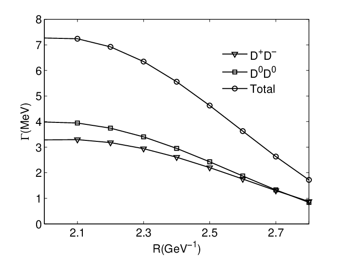
Taken to be a $1^{3}D_{3}$ $\overline{c}c$ meson, $X(3842)$ has only two strong decay channels $X(3842)\rightarrow D^{+}D^{-}$, $D^{0}\overline{D^{0}}$. From Fig.7, we can clearly see the decay width of $X(3842)$ with variations of the parameter $R$. Taking $R=2.3\sim 2.5GeV^{-1}$ discussed above, the total width of $1^{3}D_{3}$ state ranges from $5.6MeV$ to $6.9MeV$(see Fig.7). In our previous work, we have discussed the uncertainties of the results which are predicted by ${}^{3}P_{0}$ decay model. Once the optimal values of the $\gamma$ and $R$ are determined, the best predictions based on the ${}^{3}P_{0}$ decay model are expected to be within a factor of $2$Blunder; gly. More detailed analysis about the uncertainties of the results in the ${}^{3}P_{0}$ decay model can be found in Ref.gly. Considering the uncertainties of the decay model, the calculated width is roughly compatible with the experimental data $\Gamma_{X(3842)}=(2.79\pm 0.51\pm 0.35)MeV$. That is to say, it is reasonable to assign the $X(3842)$ to be the $1^{3}D_{3}$ charmonium state. Finally, we also obtain the decay ratio $\frac{\Gamma(X(3842)\rightarrow D^{+}D{-})}{X(3842)\rightarrow D^{0}\overline{D^{0}})}=0.85\sim 0.9$ for this charmonium state. This ratio can be used to make a further confirmation about this state in the future by LHCb collaboration.

References

- (1) J. J. Aubert et al., J, Phys. Rev. Lett. 33,1404(1974).
- (2) J. E. Augustin et al., Phys. Rev. Lett. 33,1406(1974).
- (3) S. K. Choi et al. Belle Collaboraion, Phys. Rev. Lett. 91, 262001(2003).
- (4) M. Tanabashi et al. (Particle Data Group), Phys. Rev. D98, 030001(2018) and 2019 update.
- (5) K. Chilikin(Belle Collaboration), Phys. Rev. D95, 112003(2017)
- (6) J. P. Lees et al. (BABAR Collaboration), Phys. Rev. D86, 072002(2012).
- (7) S. Uehara et al.(Bell Collaboration), Phys. Rev. Lett. 96, 082003(2006).
- (8) B. Aubert et al.(BABAR Collaboration), Phys. Rev. D81, 092003(2010).
- (9) K. Abe (Bell Collaboration)Phys. Rev. Lett. 98, 082001(2007).
- (10) P. Pakhlov, (Bell Collaboration) Phys. Rev. Lett. 100, 202001(2008).
- (11) P. Colangelo, F. De Fazio, S. Nicotri, Phys. Lett. B650, 166(2007).
- (12) Fulvia De Fazio, Phys. Rev. D79, 054015(2009).
- (13) V. V. Braguta, A. K. Likhoded, A. V. Luchinsky, Phys. Rev. D74, 094004(2006).
- (14) X. Liu, Z.-G. Luo, and Z.-F. Sun, Phys. Rev. Lett. 104, 122001(2010).
- (15) J. P. Lees et al. (BABAR Collaboration), Phys. Rev. D86, 072002 (2012).
- (16) F. E. Close, P. R. Page, Phys. Lett. B578, 119(2004).
- (17) M. B. Voloshin, Phys. Lett. B579, 316(2004).
- (18) C. Y. Wong, Phys. Rev. C69, 055202(2004).
- (19) E. S. Swanson, Phys. Lett. B588, 189(2004); ibid B598, 197(2004).
- (20) N. A. Tornqvist, Phys. Lett. B590, 209(2004).
- (21) Mohammad T. AlFiky, Fabrizio Gabbiani, Alexey A. Petrov, Phys.Lett. B640, 238(2006).
- (22) A. B. Larionov, M. Strikman, M. Bleicher, Phys. Lett. B749, 35(2015).
- (23) Z. G. Wang, T. Huang, Eur.Phys. J. C 74, 2891(2014).
- (24) A. Esposito, A. Pilloni, and A. D. Polosa, Phys. Rept. 668, 1(2017).
- (25) Xian-Wei Kang and J. A. Oller, arXiv:1612.08420[hep-ph](2016).
- (26) Zhi Gang Wang, Eur. Phys. J. A53, 192(2017).
- (27) Y. Cui, X. L. Chen, W. Z. Deng, S. L. Zhu, High Energy Phys. Nucl. Phys. 31, 7(2007).
- (28) R. D. Matheus, S. Narison, M. Nielsen, J. M. Richard, Phys. Rev. D75, 014005(2007).
- (29) T. W. Chiu, T. H. Hsieh, Phys. Lett. B646, 95(2007).
- (30) S. Dubnicka, A. Z. Dubnickova, M. A. Ivanov, and J. G. Korner, Phys. Rev. D81,114007(2010).
- (31) Z. G. Wang, T. Huang,Phys. Rev. D89, 054019(2014).
- (32) R. M. Albuquerque, J. M. Dias, M. Nielsen, C. M. Zanetti, Phys. Rev. D89, 076007(2014).
- (33) F. Fernandez, P. G. Ortega, D. R. Entem, AIP Conf. Proc. 1606, 168(2014).
- (34) E. J. Eichten, K. Lane, and C. Quigg, Phys. Rev. Lett. 89,162002(2002), arXiv:hep-ph/0206018.
- (35) E. J. Eichten, K. Lane, and C. Quigg, Phys. Rev. D73,014014(2006), Erratum ibid. D73, 079903(2006), arXiv:hep-ph/0511179.
- (36) T. Barnes and S. Godfrey, Phys. Rev. D69, 054008(2004), arXiv:hep-ph/0311162.
- (37) T. Barnes, S. Godfrey, and E. S. Swanson, Higher charmonia, Phys. Rev. D72, 054026(2005), arXiv:hep-ph/0505002.
- (38) S. F. Radford and W. W. Repko, Phys. Rev. D75,074031(2007), arXiv:hep-ph/0701117.
- (39) S. Godfrey and N. Isgur, Phys. Rev. D32,189(1985).
- (40) E. J. Eichten and F. Feinberg, Phys. Rev. D23, 2724(1981).
- (41) L. P. Fulcher, Phys. Rev. D44, 2079(1991).
- (42) S. N. Gupta, S. F. Radford, and W. W. Repko, Phys. Rev. D34, 201(1986).
- (43) D. Ebert, R. N. Faustov, and V. O. Galkin, Phys. Rev. D67, 014027(2003), arXiv:hep-ph/0210381.
- (44) J. Zeng, J. W. Van Orden, and W. Roberts, Phys. Rev. D52, 5229(1995), arXiv:hep-ph/9412269.
- (45) R. Aaij, et al., arXiv:1903.12240[hep-ex](2019).
- (46) M. A. Shifman, A. I. Vainshtein and V. I. Zakharov, Nucl. Phys. B147,385(1979); Nucl. Phys. B147,448(1979).
- (47) L. J. Reinders, H. Rubinstein and S. Yazaki, Phys. Rept. 127,1(1985).
- (48) Z. G. Wang, Eur. Phys. J. C75,427(2015).
- (49) S. Narison, Nucl. Part. Phys. Proc. 270, 143(2016).
- (50) H. Sundu and K. Azizi, Eur. Phys. J. A48,81(2012); K. Azizi, H. Sundu, J. Y. Sungu and N. Yinelek, Phys. Rev. D88,036005(2013); K. Azizi, Y. Sarac and H. Sundu, Eur. Phys. J. C74,3106(2014). H. A. Alhendi, T. M. Aliev and M. Savci, JHEP 1604, 050(2016).
- (51) Z. G. Wang and Z. Y. Di, Eur. Phys. J. A50, 143(2014); Z. G. Wang, Eur. Phys. J. C74, 3123(2014); Z. Y. Li, Z. G. Wang and G. L. Yu, Mod. Phys. Lett. A31, 1650036(2016).
- (52) H. G. Blundell, arXiv:hep-ph/9608473; H. G. Blundell and S. Godfrey, Phys. Rev. D53, 3700 (1996); H. G. Blundell, S. Godfrey, and B. Phelps, Phys. Rev. D53, 3712 (1996).
- (53) H. Q. Zhou, R. G. Ping, and B. S. Zou, Phys. Lett. B611, 123(2005).
- (54) D.-M. Li and S. Zhou, Phys. Rev. D78, 054013(2008); D.-M. Li and E. Wang, Eur. Phys. J. C63, 297(2009); D.-M. Li, P.-F. Ji, and B. Ma, Eur. Phys. J. C71, 1582(2011).
- (55) B. Zhang, X. Liu, W. Z. Deng, and S. L. Zhu, Eur. Phys. J. C50, 617(2007); Y. Sun, Q. T. Song, D. Y. Chen, X. Liu, and S. L. Zhu, Phys. Rev. D89, 054026(2014).
- (56) YU Guo-Liang, WANG Zhi-Gang, LI Zhen-Yu, MENG Gao-Qing, Chin. Phys. C 39, 063101(2015); Guo-Liang Yu, Zhi-Gang Wang, Zhen-Yu Li, Phys. Rev. D 94, 074024(2016).
- (57) J. J. Zhu and M. L. Yan, hep-ph/9903349; and references therein
- (58) S. Narison, Phys. Lett. B706, 412(2012); S. Narison, Phys. Lett. B707, 259(2012).
- (59) P. Colangelo and A. Khodjamirian, hep-ph/0010175
- (60) Z. G. Wang, Nucl.Phys. A957, 85(2017)
- (61) L. Micu, Nucl. Phys. B10, 521(1969).
- (62) R. Carlitz and M. Kislinger, Phys. Rev. D2, 336(1970); E. W. Colglazier and J. L. Rosner, Nucl. Phys. B27, 349(1971); W. P. Petersen and J. L. Rosner, Phys. Rev. D6, 820(1972).
- (63) A. Le Yaouanc, L. Oliver, O. Pene, and J.-C. Raynal, Phys. Rev. D8, 2223(1973); 9, 1415 (1974); 11, 1272(1975); Phys. Lett. B71, 397(1977); A. Le Yaouanc, L. Oliver, O. Pene, and J. C. Raynal, Phys. Lett. B72, 57(1977).
- (64) E. S. Ackleh, T. Barnes, and E. S. Swanson, Phys. Rev. D54, 6811(1996); T. Barnes, N. Black, and P. R. Page, Phys. Rev. D68, 054014 (2003); T. Barnes, S. Godfrey, and E. S. Swanson, Phys. Rev. D72, 054026(2005).
- (65) J. Ferretti, G. Galata, and E. Santopinto, Phys. Rev. C88, 015207(2013).
- (66) P. G. Ortega, J. Segovia, D. R. Entem and F. Fernandez, arXiv:1706.02639(2017).
- (67) J. Ferretti, G. Galata, and E. Santopinto, Phys. Rev. D90, 054010(2014).
- (68) J. Ferretti and E. Santopinto, Phys. Rev. D90, 094022(2014).
- (69) F. E. Close and E. S. Swanson, Phys. Rev. D72, 094004(2005); F. E. Close, C. E. Thomas, O. Lakhina, and E. S. Swanson, Phys. Lett. B647, 159(2007).
- (70) J. Segovia, D.R. Entem, F. Fernandez, Phys. Lett. B715, 322(2012).
- (71) Ze Zhao, Dan-Dan Ye, and Ailin Zhang,Phys. Rev. D95, 114024(2017).
- (72) Xue-wen Liu, Hong-Wei Ke, Xiang Liu, Xue-Qian Li, Eur. Phys. J. C76, 549(2016)
- (73) R. Kokoski and N. Isgur, Phys. Rev. D35, 907(1987).
- (74) S. Godfrey and R. Kokoski, Phys. Rev. D43, 1679(1991).
- (75) B-Q. Li, and K-T. Chao, Phys. Rev. D79, 094004(2009).
- (76) You-chang Yang, Zurong Xia, and Jialun Ping, Phys. Rev. D81, 094003(2010).
- (77) Guo Liang Yu, Zhi Gang Wang and Zhen Yu Li, Chinese Physics C Vol. 39(6), 063101(2015).