A nodal integration scheme for meshfree Galerkin methods using the virtual element decomposition

R. Silva-Valenzuela Affiliation: 1,2,3 A. Ortiz-Bernardin\comma\corrauth Affiliation: 1,2 N. Sukumar Affiliation: 4 E. Artioli and N. Hitschfeld-Kahler Affiliation: 5 Affiliation: 6,7 Address: \affilnum1 Department of Mechanical Engineering, Universidad de Chile, Av. Beauchef 851, Santiago 8370456, Chile
\affilnum2 Computational and Applied Mechanics Laboratory, Center for Modern Computational Engineering, Facultad de Ciencias Físicas y Matemáticas, Universidad de Chile, Av. Beauchef 851, Santiago 8370456, Chile
\affilnum3 Department of Mechanical Engineering, Universidad de La Serena, Av. Benavente 980, La Serena 1720170, Chile
\affilnum4 Department of Civil and Environmental Engineering, University of California, Davis, CA 95616, USA
\affilnum5 Department of Civil Engineering and Computer Science, University of Rome Tor Vergata, Via del Politecnico 1, 00133 Rome, Italy
\affilnum6 Department of Computer Science, Universidad de Chile, Av. Beauchef 851, Santiago 8370456, Chile
\affilnum7 Meshing for Applied Science Laboratory, Center for Modern Computational Engineering, Facultad de Ciencias Físicas y Matemáticas, Universidad de Chile, Av. Beauchef 851, Santiago 8370456, Chile

Abstract

In this paper, we present a novel nodal integration scheme for meshfree Galerkin methods that draws on the mathematical framework of the virtual element method. We adopt linear maximum-entropy basis functions for the discretization of field variables, although the proposed scheme is applicable to any linear meshfree approximant. In our approach, the weak form integrals are nodally integrated using nodal representative cells that carry the nodal displacements and state variables such as strains and stresses. The nodal integration is performed using the virtual element decomposition, wherein the bilinear form is decomposed into a consistency part and a stability part that ensure consistency and stability of the method. The performance of the proposed nodal integration scheme is assessed through benchmark problems in linear and nonlinear analyses of solids for small displacements and small-strain kinematics. Numerical results are presented for linear elastostatics and linear elastodynamics, and viscoelasticity. We demonstrate that the proposed nodally integrated meshfree method is accurate, converges optimally, and is more reliable and robust than a standard cell-based Gauss integrated meshfree method.

keywords

nodal integration, meshfree Galerkin methods, maximum-entropy approximants, virtual element method, patch test, stability

\NME

10000000

\runningheads

Silva-Valenzuela et al.A nodal integration scheme for meshfree Galerkin methods

\noreceived\norevised\noaccepted

\corraddr

A. Ortiz-Bernardin, Department of Mechanical Engineering, Universidad de Chile, Av. Beauchef 851, Santiago 8370456, Chile. E-mail: aortizb@uchile.cl

1 INTRODUCTION

Meshfree Galerkin methods are based on the weak form where the field variables are discretized using basis functions associated with a set of scattered nodes that partition the domain of analysis. Since the inception of the element-free Galerkin method [1], efficient and accurate numerical integration of the weak form integrals has attracted broad attention in meshfree Galerkin methods. The different numerical integration techniques that exist for meshfree Galerkin methods can be grouped into two main approaches: cell integration and nodal integration techniques. Nodal integration in meshfree methods is attractive since state variables (strains, stresses, and internal variables) can be stored at the nodes, thereby avoiding the need for remapping algorithms at integration points that arise in traditional Lagrangian finite element large deformation simulations with remeshing. In the optimal transportation meshfree method [2], remeshing is avoided by using the integration points as the carriers of material state information in tandem with changes in the support of the basis functions to enable Lagrangian finite deformation simulations. In the material point method [3], integration points of an initial grid (usually, a Cartesian grid) carry the material state variables and the solution stage occurs in three phases: (a) information is mapped from particles to grid nodes; (b) equations of motion are solved on the grid nodes, and the updated information is mapped back to the particles to update their positions and velocities; and (c) the grid is reset. In this process, the mesh remains fixed throughout the simulation, and the deformation causes the material points to move within other cells in the grid. In this paper, we use the virtual element decomposition [4] and follow Reference [5] to devise an accurate and stable nodally integrated meshfree method for linear elastostatics and linear elastodynamics, as well as nonlinear viscoelasticity.

The most simple cell integration technique requires the construction of nonoverlapping cells on which standard Gauss integration is performed. However, this integration scheme is inexact due to the following two properties of meshfree basis functions [6]: (1) They are nonpolynomial functions; and (2) in general, the region that is defined by the intersecting supports of two overlapping nodal basis functions does not coincide with the integration cell. These are two issues that often lead to consistency errors (patch test is not passed) and stability problems due to underintegration. Various approaches have been put forth in meshfree Galerkin methods to address integration errors on cells. For instance, higher-order tensor-product Gauss quadrature is adopted in the element-free Galerkin method [1, 6], whereas the support of the nodal basis functions is used as the domain of integration in the meshless local Petrov-Galerkin method [7] and also in the method of finite spheres [8]. More details on cell-based integration schemes in meshfree Galerkin methods can be found in Ortiz-Bernardin et al. [5].

Nodal integration techniques perform the integration of the weak form integrals by sampling them at the nodes. This approach requires the construction of nodal cells that represent the volume of the integrals being sampled at the nodes. Nodal integration techniques are also prone to integration errors and require to be stabilized. A direct nodal integration (1-point) scheme leads to rank instabilities because meshfree basis functions have zero or nearly zero derivatives at the nodes. In an effort to stabilize the rank instability, Beissel and Belytschko [9] introduced a least-squares residual-based method where the second-order derivatives stabilize the rank instability. With the aim of computing nodal derivatives away from the nodes to avoid rank instabilities, Chen et al. [10] devised a strain smoothing procedure known as stabilized conforming nodal integration (SCNI) approach, which is the cornerstone of various meshfree nodal-based [11, 12, 13] and cell-based [14, 15, 16] integration methods, and even smoothed finite element methods [17]. Another method to compute derivatives away from the nodes is the stress-point method, which was first introduced in the smoothed particle hydrodynamics (SPH) meshfree method [18]. Although the SCNI approach [10] suppresses the rank instability and provides patch test satisfaction, instabilities due to nonzero low-energy modes are still encountered [12]. Puso et al. [12] proposed a penalty stabilization to stabilize the SCNI method. Hillman and Chen [19] combined the arbitrary order variationally consistent meshfree nodal integration framework [13] with a stabilization method devised from an implicit gradient expansion of the strains at the nodes. The resulting method is first-order variationally consistent and stable, and unlike the stabilization method of Puso et al. [12], it is devoid of tunable parameters.

Recently, the virtual element method [4, 20] (VEM) has been proposed, where an exact algebraic construction of the stiffness matrix is realized without the explicit construction of basis functions (basis functions are deemed as virtual). In the VEM, the stiffness matrix is decomposed into two parts: a consistent term that reproduces a given polynomial space and a correction term that provides stability. Such a decomposition (herein referred to as the virtual element decomposition) is formulated in the spirit of the Lax equivalence theorem (consistency $+$ stability $\to$ convergence) for finite-difference schemes and is sufficient for the method to pass the patch test. In polygonal and polyhedral finite elements, Talischi and Paulino [21], Gain et al. [22] and Manzini et al. [23] have used the virtual element decomposition to pass the patch test. The VEM can be viewed as a stabilized Galerkin method on polytopal meshes [24]. For meshfree Galerkin methods with cell-based integration, Ortiz-Bernardin et al. [5] used the virtual element decomposition to develop a method for linear elastostatics that is consistent and stable.

In this paper, on using the virtual element decomposition, a novel meshfree nodal integration technique for linear and nonlinear analyses of solids for small displacements and small-strain kinematics is presented. In particular, linear elastostatics, linear elastodynamics and viscoelasticity are considered. We use the acronym NIVED to refer to this method. The distinctions and contributions of the present work vis-à-vis our prior work on meshfree Galerkin methods using the virtual element decomposition [5] are as follows:

•

focus herein is on nodal integration, whereas Gauss-like integration scheme is used in Ortiz-Bernardin et al. [5];
•

we develop the method for linear (static and dynamic) and nonlinear analyses of solids for small displacements and small-strain kinematics, whereas only linear elastostatics is treated in the prior work; and
•

unlike the prior work, the stabilization of the stiffness matrix in the nodal integration method does not require a tunable (scaling) parameter.

We consider maximum-entropy basis functions (Section 2), although the formulation is applicable to any linear meshfree approximant. The governing equations for linear elastostatics are described in Section 3. The main ingredients of the virtual element framework and the development of our proposed nodal integration technique are presented in Section 4 for linear elasticity and in Section 6 for nonlinear analysis of viscoelastic solids. The demonstration of the patch test satisfaction is provided in Section 5. The accuracy and convergence of the devised nodal integration method are assessed in Section 7 through several examples in linear elastostatics, linear elastodynamics and viscoelasticity. A summary of our main findings with some final remarks is provided in Section 8.

2 MAXIMUM-ENTROPY BASIS FUNCTIONS

Consider a convex domain represented by a set of $N$ scattered nodes and a prior (weight) function $w_{a}(\bm{x})$ associated with each node $a$ . We can write down the approximation for a vector-valued function $\bm{v}(\bm{x})$ in the form:

\bm{v}^{h}(\bm{x})=\sum_{a=1}^{m}\phi_{a}(\bm{x})\bm{v}_{a},

(1)

where $\bm{v}_{a}:=\bm{v}(\bm{x}_{a})$ are nodal coefficients, $\phi_{a}(\bm{x})$ is the meshfree basis function associated with node $a$ and $m\leq N$ represents the number of nodes whose basis functions take a nonzero value at the point $\bm{x}$ .

On using the Shannon-Jaynes (or relative) entropy functional, the maximum-entropy basis functions $\{\phi_{a}(\bm{x})\geq 0\}_{a=1}^{m}$ are obtained via the solution of the following convex optimization problem [25]:


	$\displaystyle\min_{\bm{\phi}\in{{\rm{I\!R}}}_{+}^{m}}\sum_{a=1}^{m}$	$\displaystyle\phi_{a}(\bm{x})\ln\left(\frac{\phi_{a}(\bm{x})}{w_{a}(\bm{x})}\right)$	(2a)
subject to the linear reproducing conditions:
	$\displaystyle\sum_{a=1}^{m}\phi_{a}(\bm{x})=1$	$\displaystyle\quad\sum_{a=1}^{m}\phi_{a}(\bm{x})\,\bm{c}_{a}=\bm{0},$	(2b)

where $\bm{c}_{a}=\bm{x}_{a}-\bm{x}$ are shifted nodal coordinates and ${\rm{I\!R}}_{+}^{m}$ is the nonnegative orthant. In this paper, we use as the prior weight function either the Gaussian radial basis function given by [26]

w_{a}(\bm{x})=\exp\left(-\frac{\gamma}{h_{a}^{2}}\|\bm{c}_{a}\|^{2}\right),

where $\gamma$ is a parameter that controls the support size of the basis function and $h_{a}$ is a characteristic nodal spacing associated with node $a$ , or the $C^{2}$ quartic polynomials given by [27]

w_{a}(q)=\left\{\begin{array}[]{lr}1-6q^{2}+8q^{3}-3q^{4}&\quad 0\leq q\leq 1\\ 0&\quad q>1\end{array}\right.,

(3)

where $q=\|\bm{c}_{a}\|/(\gamma h_{a})$ .

On using the method of Lagrange multipliers, the solution to (2) is given by [25]

\phi_{a}(\bm{x},\bm{\lambda})=\frac{w_{a}(\bm{x})\exp(-\bm{\lambda}(\bm{x})\cdot\bm{c}_{a}(\bm{x}))}{Z(\bm{x},\bm{\lambda}(\bm{x}))},\quad Z(\bm{x},\bm{\lambda}(\bm{x}))=\sum_{b=1}^{m}w_{b}(\bm{x})\exp(-\bm{\lambda}(\bm{x})\cdot\bm{c}_{b}(\bm{x})),

(4)

where the Lagrange multiplier vector $\bm{\lambda}(\bm{x})$ is obtained as the minimizer of the dual optimization problem ( $\bm{x}$ is fixed):

\bm{\lambda}^{*}(\bm{x})=\arg\min_{\bm{\lambda}\in{{\rm{I\!R}}}^{d}}\ln Z(\bm{x},\bm{\lambda}),

where $\bm{\lambda}^{*}$ is the converged solution that gives the basis functions as $\phi_{a}(\bm{x})=\phi_{a}(\bm{x},\bm{\lambda}^{*})$ for $a=1,\ldots,m$ .

3 GOVERNING EQUATIONS

3.1 Strong form

Consider an elastic body that occupies the open domain $\Omega\subset{\rm{I\!R}}^{2}$ and is bounded by the one-dimensional surface $\Gamma$ whose unit outward normal is $\bm{n}_{\Gamma}$ . The boundary is assumed to admit decompositions $\Gamma=\Gamma_{u}\cup\Gamma_{t}$ and $\emptyset=\Gamma_{u}\cap\Gamma_{t}$ , where $\Gamma_{u}$ is the Dirichlet boundary and $\Gamma_{t}$ is the Neumann boundary. The closure of the domain is $\overline{\Omega}=\Omega\cup\Gamma$ . Let $\bm{u}(\bm{x}):\overline{\Omega}\rightarrow{\rm{I\!R}}^{2}$ be the displacement field at a point $\bm{x}$ of the elastic body when the body is subjected to external tractions $\bar{\bm{t}}(\bm{x}):\Gamma_{t}\rightarrow{\rm{I\!R}}^{2}$ and body forces $\bm{b}(\bm{x}):\Omega\rightarrow{\rm{I\!R}}^{2}$ . The imposed Dirichlet (essential) boundary conditions are $\bar{\bm{u}}(\bm{x}):\Gamma_{u}\rightarrow{\rm{I\!R}}^{2}$ . The boundary-value problem for linear elastostatics is: find $\bm{u}(\bm{x}):\overline{\Omega}\rightarrow{\rm{I\!R}}^{2}$ such that


$\displaystyle\bm{\nabla}\cdot\bm{\sigma}+\bm{b}$	$\displaystyle=0\quad\mathrm{in}\,\,\Omega,$	(5a)
$\displaystyle\bm{u}$	$\displaystyle=\bar{\bm{u}}\quad\mathrm{on}\,\,\Gamma_{u},$	(5b)
$\displaystyle\bm{\sigma}\cdot\bm{n}_{\Gamma}$	$\displaystyle=\bar{\bm{t}}\quad\mathrm{on}\,\,\Gamma_{t},$	(5c)

where $\bm{\sigma}$ is the Cauchy stress tensor.

3.2 Weak form

The Galerkin weak formulation reads: find $\bm{u}(\bm{x})\in\mathscr{V}$ such that

\begin{split}a(\bm{u},\bm{v})&=\ell(\bm{v})\quad\forall\bm{v}(\bm{x})\in\mathscr{W},\\ a(\bm{u},\bm{v})=\int_{\Omega}\bm{\sigma}(\bm{u}):\bm{\varepsilon}(\bm{v})\,d\bm{x},&\quad\ell(\bm{v})=\int_{\Omega}\bm{b}\cdot\bm{v}\,d\bm{x}+\int_{\Gamma_{t}}\bar{\bm{t}}\cdot\bm{v}\,ds,\end{split}

(6)

where $\mathscr{V}$ and $\mathscr{W}$ are the continuous displacement trial and test spaces:

\displaystyle\mathscr{V}:=\left\{\bm{u}(\bm{x}):\bm{u}\in[H^{1}(\Omega)]^{2},\ \bm{u}=\bar{\bm{u}}\ \textrm{on }\Gamma_{u}\right\},\quad\mathscr{W}:=\left\{\bm{v}(\bm{x}):\bm{v}\in[H^{1}(\Omega)]^{2},\ \bm{v}=\bm{0}\ \textrm{on }\Gamma_{u}\right\},

and $\bm{\varepsilon}(\bm{v})$ is the small strain tensor that is given by

\bm{\varepsilon}(\bm{v})=\frac{1}{2}\left(\bm{\nabla}\bm{v}+\bm{\nabla}^{\mathsf{T}}\bm{v}\right).

(7)

We consider a set of scattered nodes that discretizes $\bar{\Omega}$ . Using these nodes, the domain $\Omega$ is partitioned into nonoverlapping nodal representative polygonal cells. This can be achieved using a Voronoi diagram (Figure 1) or a triangular mesh where the centroids of triangles surrounding a given node are connected to form a polygon (Figure 1). We denote by $E$ a node and its associated cell. The node $E$ has coordinates $\bm{x}_{E}$ in the Cartesian coordinate system and the area of its associated cell is $|E|$ .

Refer to caption — Figure 1: Construction of a nodal representative domain (shaded area) using (a) a Voronoi diagram and (b) a triangular mesh. The node and its representative cell are denoted by $E$ and $\bm{x}_{E}$ are the nodal coordinates.

A node on $\Gamma_{t}$ is denoted by $S$ and its coordinates in the Cartesian coordinate system by $\bm{x}_{S}$ . The length of influence of the node $S$ is represented by $|S|$ . Figure 2 presents two typical cases of a node located on $\Gamma_{t}$ .

The partition formed by all the nodes and their associated cells lying on $\Omega$ is denoted by $\mathcal{T}^{h}$ , where $h$ is the maximum diameter of any cell in the partition. The one-dimensional partition formed by all the nodes and their associated lengths of influence lying on $\Gamma_{t}$ is denoted by $\mathcal{E}^{h}$ .

Following a standard Galerkin procedure, we define the following discrete local spaces at the nodal cell level:

\mathscr{V}^{h}|_{E}:=\left\{\bm{u}^{h}(\bm{x}):\bm{u}^{h}\in[H^{1}(E)]^{2}\right\},\quad\mathscr{W}^{h}|_{E}:=\mathscr{V}^{h}|_{E},

where $\bm{u}^{h}(\bm{x})$ is given in the form (1) with $\bm{x}\in E$ . These discrete local spaces are assembled to form the following discrete global spaces:

	$\displaystyle\mathscr{V}^{h}$	$\displaystyle:=\left\{\bm{u}(\bm{x})\in\mathscr{V}:\bm{u}\|_{E}\in\mathscr{V}^{h}\|_{E}\quad\forall E\in\mathcal{T}^{h}\right\},$
	$\displaystyle\mathscr{W}^{h}$	$\displaystyle:=\left\{\bm{v}(\bm{x})\in\mathscr{W}:\bm{v}\|_{E}\in\mathscr{V}^{h}\|_{E}\quad\forall E\in\mathcal{T}^{h}\right\}.$

Owing to the definition of the discrete global spaces, we can evaluate the weak form (6) by sampling it locally at each node in $\mathcal{T}^{h}$ and summing through all of them, as follows:

	$a(\bm{u}^{h},\bm{v}^{h})=\sum_{E\in\mathcal{T}^{h}}a_{E}(\bm{u}^{h},\bm{v}^{h})=\sum_{E\in\mathcal{T}^{h}}\|E\|\,\bm{\varepsilon}_{E}(\bm{v}^{h}):\mathcal{D}:\bm{\varepsilon}_{E}(\bm{u}^{h})\quad\forall\bm{u}^{h},\,\forall\bm{v}^{h}\in\mathscr{V}^{h},$		(8a)
	$\ell(\bm{v}^{h})=\sum_{E\in\mathcal{T}^{h}}\ell_{b,E}(\bm{v}^{h})+\sum_{S\in\mathcal{E}^{h}}\ell_{t,S}(\bm{v}^{h})=\sum_{E\in\mathcal{T}^{h}}\|E\|\,\bm{b}_{E}\cdot\bm{v}^{h}+\sum_{S\in\mathcal{E}^{h}}\|S\|\,\bar{\bm{t}}_{S}\cdot\bm{v}^{h}\quad\forall\bm{v}^{h}\in\mathscr{V}^{h},$		(8b)

where $\mathcal{D}$ is the material moduli tensor that defines the constitutive relation $\bm{\sigma}=\mathcal{D}:\bm{\varepsilon}(\bm{u})$ ; $\bm{\varepsilon}_{E}:=\bm{\varepsilon}(\bm{x}_{E})$ , $\bm{b}_{E}:=\bm{b}(\bm{x}_{E})$ and $\bar{\bm{t}}_{S}:=\bar{\bm{t}}(\bm{x}_{S})$ are nodal quantities. Equation (8) is the result of direct nodal integration (1-point) of the weak form integrals.

4 NODAL INTEGRATION USING THE VIRTUAL ELEMENT DECOMPOSITION

As discussed in Section 1, the direct nodal integration of the bilinear form as given in (8a) is not viable due to stability issues. As a remedy, nodal integration techniques add a stabilization term to the bilinear form [12]. Here, we take a different route and develop a nodal integration scheme for meshfree methods using the mathematical framework of the virtual element method. In this approach, the consistency and stability of the nodally integrated meshfree Galerkin method is ensured by construction.

4.1 Nodal integration cell

The sampling of the weak form at an integration node in the partition $\mathcal{T}^{h}$ , where the partition is constructed by means of one of the methods shown in Figure 1, is performed using 1-point Gauss rule over the edges of its nodal cell. It is stressed that in the nodal integration scheme, the integration node and its associated nodal cell are interchangeable. This means that any quantity that is evaluated on the nodal cell is also a quantity evaluated at the node. Considering the Cartesian coordinate system, $\bm{x}_{E}$ are the coordinates of the integration node and $\bm{n}$ is the unit outward normal to the nodal cell’s boundary. A sample nodal integration cell is shown in Figure 3.

4.2 Nodal contribution

Since the NIVED method uses meshfree basis functions for the discretization of the field variables, we have to consider the contributions from the neighboring nodes when performing Gauss integration over the edges of the nodal cell. The global nodal contribution list at an integration point is defined as the global indices of the nodes whose basis functions take a nonzero value at the integration point. We label these global indices from 1 to $m$ and construct a local nodal contribution list with them. We always keep track of the correspondence between the local and global nodal contribution lists as this correspondence is used later in the assembly of the global stiffness matrix and global force vector. The construction of the local nodal contribution list is schematically shown in Figure 4 for the evaluation of meshfree basis functions at an integration point on the edge of a nodal cell.

4.3 Virtual element decomposition

Due to the nonpolynomial nature of the linearly precise maximum-entropy meshfree basis functions, the approximation of the displacement field using these functions contains a linear polynomial part plus some additional nonpolynomial terms. Let $[\mathcal{P}(E)]^{2}$ represent the space of linear displacements over the nodal cell $E$ .

Following the standard VEM literature (see for instance, Reference [28]) the following projection operator onto the linear displacement space is defined:

\Pi:\mathscr{V}^{h}|_{E}\to[\mathcal{P}(E)]^{2},\,\Pi\bm{p}=\bm{p}\ \forall\bm{p}\in[\mathcal{P}(E)]^{2},

(9)

which allows the splitting of the meshfree approximation of the fields into their linear polynomial part and their nonpolynomial terms, respectively, as follows:


$\displaystyle\bm{u}^{h}$	$\displaystyle=\Pi\bm{u}^{h}+(\bm{u}^{h}-\Pi\bm{u}^{h}),$	(10a)
$\displaystyle\bm{v}^{h}$	$\displaystyle=\Pi\bm{v}^{h}+(\bm{v}^{h}-\Pi\bm{v}^{h}).$	(10b)

The projection $\Pi$ is required to satisfy the following orthogonality condition:

a_{E}(\bm{p},\bm{v}^{h}-\Pi\bm{v}^{h})=0\quad\forall\bm{p}\in[\mathcal{P}(E)]^{2},\ \ \bm{v}^{h}\in\mathscr{V}^{h}|_{E}.

(11)

Using (10) and (11), we obtain the following decomposition of the local bilinear form:

a_{E}(\bm{u}^{h},\bm{v}^{h})=a_{E}(\Pi\bm{u}^{h},\Pi\bm{v}^{h})+a_{E}(\bm{u}^{h}-\Pi\bm{u}^{h},\bm{v}^{h}-\Pi\bm{v}^{h}).

(12)

The first term on the right-hand side of (12) is computable as it depends on the linear fields. However, the second term is noncomputable as it depends on the nonpolynomial terms. In the framework of the VEM, the second term is approximated by a bilinear form that can be conveniently computed adopting the form of a stabilization term. We denote this stability bilinear form by $s_{E}$ and rewrite (12) as follows:

a^{h}_{E}(\bm{u}^{h},\bm{v}^{h})=a_{E}(\Pi\bm{u}^{h},\Pi\bm{v}^{h})+s_{E}(\bm{u}^{h}-\Pi\bm{u}^{h},\bm{v}^{h}-\Pi\bm{v}^{h}).

(13)

We refer to (13) as the virtual element decomposition.

The virtual element decomposition is endowed with the following crucial properties for establishing the convergence of the VEM [4, 20]:

For all $h$ and for all $E$ in $\mathcal{T}^{h}$

•

Consistency: For all $\bm{p}\in[\mathcal{P}(E)]^{2}$ and for all $\bm{v}^{h}\in\mathscr{V}^{h}|_{E}$

$a_{E}^{h}(\bm{p},\bm{v}^{h})=a_{E}(\bm{p},\bm{v}^{h}).$ (14)

•

Stability: There exists two constants $\alpha_{*}>0$ and $\alpha^{*}>0$ , independent of $h$ and of $E$ , such that

\forall\bm{v}^{h}\in\mathscr{V}^{h}|_{E},\quad\alpha_{*}a_{E}(\bm{v}^{h},\bm{v}^{h})\leq a_{E}^{h}(\bm{v}^{h},\bm{v}^{h})\leq\alpha^{*}a_{E}(\bm{v}^{h},\bm{v}^{h}).

(15)

In view of the preceding properties, it is straightforward to recognize that the first term on the right-hand side of (13) provides consistency (i.e., ensures patch test satisfaction) and the second term lends stability. The stability property (15) reveals the necessary conditions that $s_{E}$ must possess: it must be symmetric and positive definite on the kernel of $\Pi$ so that property (15) holds without violating (14).

4.4 Projection operator

The explicit form of the projection operator $\Pi$ is obtained from the orthogonality condition (11). Let the strain tensor (7) be written as

\bm{\varepsilon}(\bm{v})=\bm{\nabla}\bm{v}-\bm{\omega}(\bm{v}),

(16)

where $\bm{\omega}(\bm{v})$ is the skew-symmetric tensor given by

\bm{\omega}(\bm{v})=\frac{1}{2}\left(\bm{\nabla}\bm{v}-\bm{\nabla}^{\mathsf{T}}\bm{v}\right).

(17)

Using (16), noting that $\bm{\sigma}(\bm{p})$ and $\bm{\nabla}\Pi\bm{v}^{h}$ are constant fields over $E$ since $\bm{p},\,\Pi\bm{v}^{h}\in[\mathcal{P}(E)]^{2}$ , and that $\bm{\sigma}:\bm{\omega}=0$ , we can write the orthogonality condition (11) as

$\displaystyle a_{E}(\bm{p},\bm{v}^{h}-\Pi\bm{v}^{h})$	$\displaystyle=\int_{E}\bm{\sigma}(\bm{p}):\left[\bm{\nabla}(\bm{v}^{h}-\Pi\bm{v}^{h})-\bm{\omega}(\bm{v}^{h}-\Pi\bm{v}^{h})\right]\,d\bm{x}$
	$\displaystyle=\bm{\sigma}(\bm{p}):\left[\int_{E}\bm{\nabla}\bm{v}^{h}\,d\bm{x}-\bm{\nabla}\Pi\bm{v}^{h}\int_{E}\,d\bm{x}\right]$
	$\displaystyle=\bm{\sigma}(\bm{p}):\left[\int_{E}\bm{\nabla}\bm{v}^{h}\,d\bm{x}-\|E\|\bm{\nabla}\Pi\bm{v}^{h}\right]$	(18)
	$\displaystyle=0,$	(19)

which leads to

\bm{\nabla}\Pi\bm{v}^{h}=\frac{1}{|E|}\int_{E}\bm{\nabla}\bm{v}^{h}\,d\bm{x}.

(20)

Note that (20) defines $\bm{\nabla}\Pi\bm{v}^{h}$ as the average value of $\bm{\nabla}\bm{v}^{h}$ over the cell $E$ . On using (16), (20) can be rewritten as

\bm{\nabla}\Pi\bm{v}^{h}=\bm{\varepsilon}(\Pi\bm{v}^{h})+\bm{\omega}(\Pi\bm{v}^{h})=\frac{1}{|E|}\int_{E}\bm{\varepsilon}(\bm{v}^{h})\,d\bm{x}+\frac{1}{|E|}\int_{E}\bm{\omega}(\bm{v}^{h})\,d\bm{x},

(21)

which on integrating yields

\Pi\bm{v}^{h}=\left(\frac{1}{|E|}\int_{E}\bm{\varepsilon}(\bm{v}^{h})\,d\bm{x}\right)\cdot\bm{x}+\left(\frac{1}{|E|}\int_{E}\bm{\omega}(\bm{v}^{h})\,d\bm{x}\right)\cdot\bm{x}+\bm{a}_{0}.

(22)

To determine $\bm{a}_{0}$ we need a projection operator onto constants $P_{0}:\mathscr{V}^{h}|_{E}\to{\rm{I\!R}}^{2}$ such that

P_{0}(\Pi\bm{v}^{h})=P_{0}\bm{v}^{h}.

(23)

Given that the field variables computed at the integration node become the representative field variables of the cell, we define the projection operator onto constant as

P_{0}\bm{v}^{h}=\bm{v}^{h}(\bm{x}_{E})=\bm{v}_{E},

(24)

where $\bm{x}_{E}$ are the coordinates of the integration node (see Figure 3).

Applying (23) to (22) gives

	$\displaystyle P_{0}(\Pi\bm{v}^{h})$	$\displaystyle=\left(\frac{1}{\|E\|}\int_{E}\bm{\varepsilon}(\bm{v}^{h})\,d\bm{x}\right)\cdot P_{0}\bm{x}+\left(\frac{1}{\|E\|}\int_{E}\bm{\omega}(\bm{v}^{h})\,d\bm{x}\right)\cdot P_{0}\bm{x}+P_{0}\bm{a}_{0}=P_{0}\bm{v}^{h}$
		$\displaystyle=\left(\frac{1}{\|E\|}\int_{E}\bm{\varepsilon}(\bm{v}^{h})\,d\bm{x}\right)\cdot\bm{x}_{E}+\left(\frac{1}{\|E\|}\int_{E}\bm{\omega}(\bm{v}^{h})\,d\bm{x}\right)\cdot\bm{x}_{E}+\bm{a}_{0}=\bm{v}_{E}.$		(25)

On solving for $\bm{a}_{0}$ in (4.4), we obtain

\bm{a}_{0}=\bm{v}_{E}-\left(\frac{1}{|E|}\int_{E}\bm{\varepsilon}(\bm{v}^{h})\,d\bm{x}\right)\cdot\bm{x}_{E}-\left(\frac{1}{|E|}\int_{E}\bm{\omega}(\bm{v}^{h})\,d\bm{x}\right)\cdot\bm{x}_{E}.

(26)

We introduce the definitions $\bm{\varepsilon}_{E}(\bm{v}^{h}):=\frac{1}{|E|}\int_{E}\bm{\varepsilon}(\bm{v}^{h})\,d\bm{x}$ and $\bm{\omega}_{E}(\bm{v}^{h}):=\frac{1}{|E|}\int_{E}\bm{\omega}(\bm{v}^{h})\,d\bm{x}$ since both are constant tensors over the cell and thus they can be associated with the integration node. Finally, substituting (26) into (22) yields the projection operator onto the linear displacements, as follows:

\Pi\bm{v}^{h}=\bm{\varepsilon}_{E}(\bm{v}^{h})\cdot(\bm{x}-\bm{x}_{E})+\bm{\omega}_{E}(\bm{v}^{h})\cdot(\bm{x}-\bm{x}_{E})+\bm{v}_{E}.

(27)

In (27), the cell averages $\bm{\varepsilon}_{E}(\bm{v}^{h})$ and $\bm{\omega}_{E}(\bm{v}^{h})$ are evaluated on the boundary of $E$ by invoking the divergence theorem, which gives the following nodal measures:

\bm{\varepsilon}_{E}(\bm{v}^{h})=\frac{1}{|E|}\int_{E}\bm{\varepsilon}(\bm{v}^{h})\,d\bm{x}=\frac{1}{2|E|}\int_{\partial E}\left(\bm{v}^{h}\otimes\bm{n}+\bm{n}\otimes\bm{v}^{h}\right)\,ds

(28)

and

\bm{\omega}_{E}(\bm{v}^{h})=\frac{1}{|E|}\int_{E}\bm{\omega}(\bm{v}^{h})\,d\bm{x}=\frac{1}{2|E|}\int_{\partial E}\left(\bm{v}^{h}\otimes\bm{n}-\bm{n}\otimes\bm{v}^{h}\right)\,ds,

(29)

respectively.

4.5 Projection matrix

After some algebraic manipulations, (27) can be written as

\Pi\bm{v}^{h}=\bm{h}(\bm{x})\bm{\upvarepsilon}_{E}(\bm{v}^{h})+\bm{g}(\bm{x})\bm{r}_{E}(\bm{v}^{h}),

(30)

where

\bm{h}(\bm{x})=\left[\begin{array}[]{ccccccccccccccccccccccccccccccccccccccccccccccccccc}(x_{1}-x_{1E})&0&\frac{1}{2}(x_{2}-x_{2E})\\ 0&(x_{2}-x_{2E})&\frac{1}{2}(x_{1}-x_{1E})\\ \end{array}\right],\quad\bm{g}(\bm{x})=\left[\begin{array}[]{ccccccccccccccccccccccccccccccccccccccccccccccccccc}1&0&\frac{1}{2}(x_{2}-x_{2E})\\ 0&1&-\frac{1}{2}(x_{1}-x_{1E})\\ \end{array}\right],

(31)

\bm{\upvarepsilon}_{E}(\bm{v}^{h})=\left[\begin{array}[]{ccccccccccccccccccccccccccccccccccccccccccccccccccc}(\bm{\varepsilon}_{E})_{11}&(\bm{\varepsilon}_{E})_{22}&2(\bm{\varepsilon}_{E})_{12}\\ \end{array}\right]^{\mathsf{T}},\quad\bm{r}_{E}(\bm{v}^{h})=\left[\begin{array}[]{ccccccccccccccccccccccccccccccccccccccccccccccccccc}v_{1E}&v_{2E}&2(\bm{\omega}_{E})_{12}\\ \end{array}\right]^{\mathsf{T}}.

(32)

Using meshfree basis functions leads to the following discrete representation of (31):

\bm{h}^{h}(\bm{x})=\sum_{a=1}^{m}\phi_{a}(\bm{x})\bm{h}(\bm{x}_{a})=\bm{N}\bm{H}_{E},\quad\bm{g}^{h}(\bm{x})=\sum_{a=1}^{m}\phi_{a}(\bm{x})\bm{g}(\bm{x}_{a})=\bm{N}\bm{G}_{E},\quad

(33)

where

\bm{H}_{E}=\left[\begin{array}[]{ccccccccccccccccccccccccccccccccccccccccccccccccccc}(\bm{H}_{E})_{1}\\ \vdots\\ (\bm{H}_{E})_{a}\\ \vdots\\ (\bm{H}_{E})_{m}\\ \end{array}\right],\quad(\bm{H}_{E})_{a}=\left[\begin{array}[]{ccccccccccccccccccccccccccccccccccccccccccccccccccc}(x_{1a}-x_{1E})&0&\frac{1}{2}(x_{2a}-x_{2E})\\ 0&(x_{2a}-x_{2E})&\frac{1}{2}(x_{1a}-x_{1E})\\ \end{array}\right],

(34)

\bm{G}_{E}=\left[\begin{array}[]{ccccccccccccccccccccccccccccccccccccccccccccccccccc}(\bm{G}_{E})_{1}\\ \vdots\\ (\bm{G}_{E})_{a}\\ \vdots\\ (\bm{G}_{E})_{m}\\ \end{array}\right],\quad(\bm{G}_{E})_{a}=\left[\begin{array}[]{ccccccccccccccccccccccccccccccccccccccccccccccccccc}1&0&\frac{1}{2}(x_{2a}-x_{2E})\\ 0&1&-\frac{1}{2}(x_{1a}-x_{1E})\\ \end{array}\right],

(35)

\bm{N}=\left[\begin{array}[]{ccccccccccccccccccccccccccccccccccccccccccccccccccc}\bm{N}_{1}&\cdots&\bm{N}_{a}&\cdots&\bm{N}_{m}\\ \end{array}\right],\quad\bm{N}_{a}=\left[\begin{array}[]{ccccccccccccccccccccccccccccccccccccccccccccccccccc}\phi_{a}&0\\ 0&\phi_{a}\\ \end{array}\right],

(36)

and explicitly replacing $\bm{v}^{h}$ in the form (1) into (32) gives

\bm{\upvarepsilon}_{E}^{h}=\bm{\upvarepsilon}_{E}\left(\sum_{a=1}^{m}\phi_{a}(\bm{x})\bm{v}_{a}\right)=\bm{W}_{E}^{\mathsf{T}}\bm{q},\quad\bm{r}_{E}^{h}=\bm{r}_{E}\left(\sum_{a=1}^{m}\phi_{a}(\bm{x})\bm{v}_{a}\right)=\bm{R}_{E}^{\mathsf{T}}\bm{q},

(37)

where

\bm{q}=\left[\begin{array}[]{ccccccccccccccccccccccccccccccccccccccccccccccccccc}\bm{v}_{1}^{\mathsf{T}}&\cdots&\bm{v}_{a}^{\mathsf{T}}&\cdots&\bm{v}_{m}^{\mathsf{T}}\\ \end{array}\right]^{\mathsf{T}},\quad\bm{v}_{a}=\left[\begin{array}[]{ccccccccccccccccccccccccccccccccccccccccccccccccccc}v_{1a}&v_{2a}\\ \end{array}\right]^{\mathsf{T}},

(38)

\bm{W}_{E}=\left[\begin{array}[]{ccccccccccccccccccccccccccccccccccccccccccccccccccc}(\bm{W}_{E})_{1}\\ \vdots\\ (\bm{W}_{E})_{a}\\ \vdots\\ (\bm{W}_{E})_{m}\\ \end{array}\right],\quad(\bm{W}_{E})_{a}=\left[\begin{array}[]{ccccccccccccccccccccccccccccccccccccccccccccccccccc}q_{1a}&0&q_{2a}\\ 0&q_{2a}&q_{1a}\\ \end{array}\right],\quad q_{ia}=\frac{1}{|E|}\int_{\partial E}\phi_{a}(\bm{x})n_{i}\,ds,\quad i=1,2

(39)

and

\bm{R}_{E}=\left[\begin{array}[]{ccccccccccccccccccccccccccccccccccccccccccccccccccc}(\bm{R}_{E})_{1}\\ \vdots\\ (\bm{R}_{E})_{a}\\ \vdots\\ (\bm{R}_{E})_{m}\\ \end{array}\right],\quad(\bm{R}_{E})_{a}=\left[\begin{array}[]{ccccccccccccccccccccccccccccccccccccccccccccccccccc}\phi_{a}^{E}&0&q_{2a}\\ 0&\phi_{a}^{E}&-q_{1a}\\ \end{array}\right],\quad

(40)

where $\phi_{a}^{E}:=\phi_{a}(\bm{x}_{E})$ is the value of the $a$ -th basis function at the integration node $E$ . To evaluate $q_{ia}$ in (39), a 1-point Gauss rule is used on each edge of the nodal cell (see Figure 3).

Finally, substituting (33) and (37) into (30) yields the following discrete version of the projection operator:

\Pi\bm{v}^{h}=\bm{N}\bm{H}_{E}\bm{W}_{E}^{\mathsf{T}}\bm{q}+\bm{N}\bm{G}_{E}\bm{R}_{E}^{\mathsf{T}}\bm{q}=\bm{N}(\bm{H}_{E}\bm{W}_{E}^{\mathsf{T}}+\bm{G}_{E}\bm{R}_{E}^{\mathsf{T}})\bm{q},

(41)

which defines the projection matrix (the matrix form of $\Pi$ ) as

\bm{P}_{E}=\bm{H}_{E}\bm{W}_{E}^{\mathsf{T}}+\bm{G}_{E}\bm{R}_{E}^{\mathsf{T}}.

(42)

4.6 Nodally integrated stiffness matrix

The nodally integrated local stiffness matrix is obtained by discretizing the virtual element decomposition (13). We start by working on the consistency term (i.e., the first term on the right-hand side of (13)). On using (27) to obtain $\bm{\nabla}\Pi\bm{v}^{h}=\bm{\varepsilon}_{E}(\bm{v}^{h})+\bm{\omega}_{E}(\bm{v}^{h})$ and considering the constitutive relation $\bm{\sigma}(\Pi\bm{u}^{h})=\mathcal{D}:\bm{\varepsilon}_{E}(\bm{u}^{h})$ , we can write

	$\displaystyle a_{E}(\Pi\bm{u}^{h},\Pi\bm{v}^{h})$	$\displaystyle=\|E\|\bm{\sigma}(\Pi\bm{u}^{h}):\bm{\nabla}\Pi\bm{v}^{h}$
		$\displaystyle=\|E\|\,\bm{\varepsilon}_{E}(\bm{v}^{h}):\mathcal{D}:\bm{\varepsilon}_{E}(\bm{u}^{h}).$		(43)

Using the symmetry of tensors $\bm{\varepsilon}_{E}$ and $\mathcal{D}$ , (4.6) can be written in Voigt notation as

a_{E}(\Pi\bm{u}^{h},\Pi\bm{v}^{h})=|E|\,\bm{\upvarepsilon}_{E}^{\mathsf{T}}(\bm{v}^{h})\,\bm{D}\,\bm{\upvarepsilon}_{E}(\bm{u}^{h}),

(44)

where $\bm{D}$ is the constitutive matrix for an isotropic linear elastic material given by

\bm{D}=\frac{E_{\mathrm{Y}}}{(1+\nu)(1-2\nu)}\left[\begin{array}[]{ccccccccccccccccccccccccccccccccccccccccccccccccccc}1-\nu&\nu&0\\ \nu&1-\nu&0\\ 0&0&\frac{1-2\nu}{2}\\ \end{array}\right],\quad\bm{D}=\frac{E_{\mathrm{Y}}}{1-\nu^{2}}\left[\begin{array}[]{ccccccccccccccccccccccccccccccccccccccccccccccccccc}1&\nu&0\\ \nu&1&0\\ 0&0&\frac{1-\nu}{2}\\ \end{array}\right]

(45)

for plane strain and plane stress conditions, respectively, where $E_{\mathrm{Y}}$ is the Young’s modulus and $\nu$ is the Poisson’s ratio; $\bm{\upvarepsilon}_{E}(\bm{v}^{h})$ is defined in (32).

Now, substituting the discrete version of $\bm{\upvarepsilon}_{E}(\bm{v}^{h})$ as given in (37) into (44) leads to the following discrete local consistency bilinear form:

a_{E}(\Pi\bm{u}^{h},\Pi\bm{v}^{h})=\bm{q}^{\mathsf{T}}|E|\,\bm{W}_{E}\,\bm{D}\,\bm{W}_{E}^{\mathsf{T}}\bm{d},

(46)

where $\bm{d}$ is a column vector similar to $\bm{q}$ given in (38) that contains the nodal coefficients that are associated with the displacement trial functions.

The discrete local stability bilinear form is obtained by replacing the field discretizations $\bm{u}^{h}=\bm{N}\bm{d}$ and $\bm{v}^{h}=\bm{N}\bm{q}$ , where $\bm{N}$ is defined in (36), along with (41) into the second term on the right-hand side of (13). This yields

	$\displaystyle s_{E}(\bm{u}^{h}-\Pi\bm{u}^{h},\bm{v}^{h}-\Pi\bm{v}^{h})$	$\displaystyle=s_{E}(\bm{N}\bm{d}-\bm{N}\bm{P}_{E}\bm{d},\bm{N}\bm{q}-\bm{N}\bm{P}_{E}\bm{q})$
		$\displaystyle=\bm{q}^{\mathsf{T}}(\bm{I}_{2m}-\bm{P}_{E})^{\mathsf{T}}\,\bm{S}_{E}\,(\bm{I}_{2m}-\bm{P}_{E})\,\bm{d},$		(47)

where $\bm{I}_{2m}$ is the identity ( $2m\times 2m$ ) matrix and $\bm{S}_{E}=s_{E}(\bm{N}^{\mathsf{T}},\bm{N})$ . Thus, substituting (46) and (4.6) into the first and second terms on the right-hand side of (13), respectively, gives

a_{E}^{h}(\bm{u}^{h},\bm{v}^{h})=\bm{q}^{\mathsf{T}}\left(|E|\,\bm{W}_{E}\,\bm{D}\,\bm{W}_{E}^{\mathsf{T}}+(\bm{I}_{2m}-\bm{P}_{E})^{\mathsf{T}}\,\bm{S}_{E}\,(\bm{I}_{2m}-\bm{P}_{E})\right)\bm{d},

(48)

which defines the nodally integrated local stiffness matrix as the sum of the consistency stiffness matrix $\bm{K}_{E}^{\mathrm{c}}$ and the stability stiffness matrix $\bm{K}_{E}^{\mathrm{s}}$ , as follows:

\bm{K}_{E}=\bm{K}_{E}^{\mathrm{c}}+\bm{K}_{E}^{\mathrm{s}},\quad\bm{K}_{E}^{\mathrm{c}}=|E|\,\bm{W}_{E}\,\bm{D}\,\bm{W}_{E}^{\mathsf{T}},\quad\bm{K}_{E}^{\mathrm{s}}=(\bm{I}_{2m}-\bm{P}_{E})^{\mathsf{T}}\,\bm{S}_{E}\,(\bm{I}_{2m}-\bm{P}_{E}).

(49)

Regarding the stability stiffness, we make the following choice for $\bm{S}_{E}$ :

\bm{S}_{E}=\bm{I}_{2m}\odot\left(\bm{1}_{2m}\otimes\bm{\gamma}\right),

(50)

where $\bm{1}_{2m}$ is the unit ( $2m\times 1$ ) column vector, $\bm{\gamma}=\mathrm{diag}(\bm{K}_{E}^{\mathrm{c}})$ is a column vector containing the diagonal of the matrix $\bm{K}_{E}^{\mathrm{c}}$ and $\odot$ is the element-wise product. This means that $\bm{S}_{E}$ is a diagonal matrix whose diagonal entries are those of the diagonal of the nodally integrated local consistency stiffness matrix, which is in the spirit of the “ $D$ -recipe” studied in References [29, 30].

4.7 Nodally integrated force vector

For linear fields, the simplest approximation for the body force vector is constructed by projecting both the body force vector $\bm{b}$ and the test displacements $\bm{v}^{h}$ onto constants, as follows [4, 20, 31]:

\ell_{b,E}^{h}(\bm{v}^{h})=\int_{E}P_{0}\bm{b}^{h}\cdot P_{0}\bm{v}^{h}\,d\bm{x}=P_{0}\bm{b}^{h}\cdot P_{0}\bm{v}^{h}\int_{E}\,d\bm{x}=|E|\,\bm{b}_{E}\cdot\bm{v}_{E}=\bm{q}^{\mathsf{T}}|E|\bm{N}_{E}^{\mathsf{T}}\bm{b}_{E},

(51)

where we have used $P_{0}$ as defined in (24), and

\bm{N}_{E}=\left[(\bm{N}_{E})_{1}\quad\cdots\quad(\bm{N}_{E})_{a}\quad\cdots\quad(\bm{N}_{E})_{m}\right],\quad(\bm{N}_{E})_{a}=\left[\begin{array}[]{ccccccccccccccccccccccccccccccccccccccccccccccccccc}\phi_{a}^{E}&0\\ 0&\phi_{a}^{E}\\ \end{array}\right],

(52)

where $\phi_{a}^{E}$ is defined below (40). Hence, the nodal body force vector is given by

\bm{f}_{b,E}=|E|\,\bm{N}_{E}^{\mathsf{T}}\bm{b}_{E},

(53)

which coincides with the direct integration of the body force vector at the node with coordinates $\bm{x}_{E}$ .

The integral that defines the traction force vector is similar to the integral that defines the body force vector, but it is one dimension lower. This means that we can simply apply a direct nodal integration on the Neumann edges. Proceeding likewise leads to the following nodal traction force vector:

\bm{f}_{t,S}=|S|\,\bm{N}_{S}^{\mathsf{T}}\bar{\bm{t}}_{S},

(54)

where

\bm{N}_{S}=\left[(\bm{N}_{S})_{1}\quad\cdots\quad(\bm{N}_{S})_{a}\quad\cdots\quad(\bm{N}_{S})_{m}\right],\quad(\bm{N}_{S})_{a}=\left[\begin{array}[]{ccccccccccccccccccccccccccccccccccccccccccccccccccc}\phi_{a}^{S}&0\\ 0&\phi_{a}^{S}\\ \end{array}\right]

(55)

with $\phi_{a}^{S}:=\phi_{a}(\bm{x}_{S})$ .

4.8 Nodally integrated mass matrix

With the aim of testing the NIVED approach for an elastodynamic problem, we show how to compute the approximation of the mass matrix using the virtual element decomposition. The mass matrix is constructed along the same lines as the stiffness matrix, that is, the mass matrix is split into a consistency part and a stability part. However, this construction is done using an $L^{2}$ -projection on $[\mathcal{P}(E)]^{2}$ of any function $\bm{v}^{h}\in[\mathcal{W}(E)]^{2}$ . For linear and quadratic fields, the $L^{2}$ -projection coincides with the elliptic projection $\Pi$ [32, 28]. This means,

\int_{E}\phi_{a}\phi_{b}d\bm{x}=\int_{E}\Pi\phi_{a}\Pi\phi_{b}d\bm{x}+\int_{E}(\phi_{a}-\Pi\phi_{a})(\phi_{b}-\Pi\phi_{b}).

For testing our nodal integration approach, we use Newmark’s constant average acceleration time integration method, which is implicit and unconditionally stable. For such integrators, the stability part of the mass matrix is not needed [33]. Thus, generally we only require the consistency term $\int_{E}\Pi\phi_{a}\Pi\phi_{b}\,d\bm{x}$ . Hence, the expression for the nodally integrated mass matrix for a solid material of density $\rho$ , is:

\bm{M}_{E}=\rho|E|\int_{E}\bm{P}^{\mathsf{T}}\bm{N}^{\mathsf{T}}\bm{N}\bm{P}\,d\bm{x}=\rho|E|\bm{P}^{\mathsf{T}}\left(\int_{E}\bm{N}^{\mathsf{T}}\bm{N}\,d\bm{x}\right)\bm{P}=\rho|E|\bm{P}^{\mathsf{T}}\bm{N}_{E}^{\mathsf{T}}\bm{N}_{E}\bm{P},

(56)

where the integral has been nodally integrated at $\bm{x}_{E}$ leading to $\bm{N}_{E}$ as defined in (52).

For a detailed treatment of time-dependent problems using the virtual element framework, the interested reader is referred to References [33, 34, 35].

5 PATCH TEST SATISFACTION

In the patch test, the exact linear field $\bm{u}(\bm{x})=\bm{p}(\bm{x})\in[\mathcal{P}(E)]^{2}$ is imposed on the entire boundary of the domain. Hence, the numerical solution for the patch test must be $\bm{u}^{h}(\bm{x})=\bm{p}(\bm{x})$ on the whole domain. Using this in (13), we get

a_{E}(\bm{p},\bm{v}^{h})=a_{E}(\Pi\bm{p},\Pi\bm{v}^{h})+a_{E}(\bm{p}-\Pi\bm{p},\bm{v}^{h}-\Pi\bm{v}^{h}).

(57)

The second term on the right-handside of (57) is zero because $\bm{p}-\Pi\bm{p}=\bm{p}-\bm{p}=0$ . Then,

a_{E}(\bm{p},\bm{v}^{h})=\int_{E}\bm{\sigma}(\bm{p}):\bm{\varepsilon}(\Pi\bm{v}^{h})\,d\bm{x}.

(58)

Note that $\bm{\sigma}(\bm{p})$ is a constant field. Let $\bm{\sigma}^{c}$ denote this constant stress field and observe that $\bm{\varepsilon}(\Pi\bm{v}^{h})=\bm{\varepsilon}_{E}(\bm{v}^{h})$ is the nodal strain (cell average) defined in (28) and thus a constant field as well. Hence, (58) becomes

a_{E}(\bm{p},\bm{v}^{h})=|E|\bm{\sigma}^{c}:\bm{\varepsilon}_{E}(\bm{v}^{h})=\bm{\sigma}^{c}:\frac{1}{2}\int_{\partial E}\left(\bm{v}^{h}\otimes\bm{n}+\bm{n}\otimes\bm{v}^{h}\right)\,ds.

(59)

We now substitute $\bm{v}^{h}(\bm{x})=\phi_{a}(\bm{x})\bm{v}_{a}$ into (59) and sum over all the nodal cells to obtain

\sum_{E\in\mathcal{T}^{h}}a_{E}(\bm{p},\bm{v}^{h})=\sum_{E\in\mathcal{T}^{h}}\left(\int_{\partial E}\bm{B}_{a}\bm{\sigma}^{c}\,ds\right)\bm{v}_{a}=\bm{f}_{a}\cdot\bm{v}_{a},

(60)

where

\bm{B}_{a}=\left[\begin{array}[]{ccccccccccccccccccccccccccccccccccccccccccccccccccc}\phi_{a}n_{1}&0\\ 0&\phi_{a}n_{2}\\ \phi_{a}n_{2}&\phi_{a}n_{1}\\ \end{array}\right],

(61)

and $\bm{f}_{a}$ is an interior nodal force. Since the patch test produces a state of constant strains and stresses, all the interior nodal forces must be identically equal to zero. Therefore, for the patch test to be satisfied it suffices to show that

\bm{f}_{a}=\sum_{E\in\mathcal{T}^{h}}\int_{\partial E}\bm{B}_{a}\bm{\sigma}^{c}\,ds=\bm{0},

(62)

where the assembly is over all the nodal cells that have a non-zero intersection with the support of $\phi_{a}$ . To compute (62), we choose a 1-point Gauss rule over the edges of the integration cells, and since the evaluation of $\bm{B}_{a}$ at a given interior edge will arise from two adjacent cells in the assembly, the two contributions cancel each other. Thus, the net contribution to $\bm{f}_{a}$ from all the interior edges vanishes, and hence (62) is satisfied.

6 EXTENSION TO NONLINEAR ANALYSIS: THE VISCOELASTIC CASE

In this section, the proposed NIVED scheme is extended to solid mechanics problems in which the constitutive law for the solid material depends on the history of deformation. In particular, we consider the case of Generalized Maxwell viscoelastic model describing a standard linear isotropic solid [36], wherein the Cauchy stress in vector form and as a function of time $t$ is split as

\bm{\upsigma}(t)=\bm{s}(t)+\bm{m}K\bm{m}^{\mathsf{T}}\bm{\upvarepsilon},

(63)

where $K$ is the material’s Bulk modulus, $\bm{\upvarepsilon}$ is the small strain tensor in vector form, $\bm{m}=[1\quad 1\quad 0]^{\mathsf{T}}$ and $\bm{s}(t)$ is the deviatoric stress given by

\bm{s}(t)=\int_{-\infty}^{t}2G(t-t^{\prime})\frac{\partial\bm{e}}{\partial t^{\prime}}\,dt^{\prime},

(64)

where $\bm{e}=\bm{\upvarepsilon}-1/3\,\bm{m}\bm{m}^{\mathsf{T}}\bm{\upvarepsilon}$ is the deviatoric strain and $G(t)$ is the shear relaxation modulus given by a one-term Prony series that is of the form

G(t)=G[\mu_{0}+\mu_{1}\exp(-t/\lambda_{1})],

(65)

where $G=E/(2(1+\nu))$ , $\mu_{0}>0$ and $\mu_{1}>0$ are parameters that satisfy $\mu_{0}+\mu_{1}=1$ , and $\lambda_{1}$ is a relaxation time. Substituting (65) into (64) leads to

\bm{s}(t)=2G\left[\mu_{0}\bm{e}(t)+\mu_{1}\bm{q}^{(1)}(t)\right],

(66)

where $\bm{q}^{(1)}(t)$ is the dimensionless partial deviatoric strain given by

\bm{q}^{(1)}(t)=\int_{-\infty}^{t}\exp(-(t-t^{\prime})/\lambda_{1})\frac{\partial\bm{e}}{\partial t^{\prime}}\,dt^{\prime}.

(67)

The term $\bm{q}^{(1)}(t)$ is solved using the recursion formula [36]

\bm{q}_{n+1}^{(1)}=\exp(-\Delta t/\lambda_{1})\bm{q}_{n}^{(1)}+\Delta\bm{q}_{n+1}^{(1)},

(68)

where

\Delta\bm{q}_{n+1}^{(1)}=\frac{\lambda_{1}}{\Delta t}(1-\exp(-\Delta t/\lambda_{1}))(\bm{e}_{n+1}-\bm{e}_{n}).

(69)

Thus, using the recursion formula, the stresses can be written as

\bm{s}_{n+1}=2G\left[\mu_{0}\bm{e}_{n+1}+\mu_{1}\bm{q}_{n+1}^{(1)}\right],

(70)

and

\bm{\upsigma}_{n+1}=\bm{s}_{n+1}+\bm{m}K\bm{m}^{\mathsf{T}}\bm{\upvarepsilon}_{n+1}.

(71)

On considering (71) along with (70) and (68), it is realized that $\bm{\upsigma}_{n+1}$ is determined by the knowledge of the time increment $\Delta t$ and the strain $\bm{\upvarepsilon}$ at times $t_{n}$ and $t_{n+1}$ .

The numerical solution of the equilibrium equation for the standard linear isotropic solid described by the Generalized Maxwell viscoelastic model is sought incrementally using a Newton-Raphson scheme. Under the NIVED framework, the constitutive equation (71) is computed using the vector form of the nodal strain (28) and the base equilibrium equation for the Newton-Raphson scheme is obtained by linearizing the following VED representation of the virtual work:

		$\displaystyle\|E\|\,\bm{\upvarepsilon}_{E}^{\mathsf{T}}(\bm{v}^{h})\bm{\upsigma}_{n+1}(\bm{\upvarepsilon}_{E}(\bm{u}_{n+1}^{h}))+\int_{E}\left[\bm{\upvarepsilon}(\bm{v}^{h})-\bm{\upvarepsilon}_{E}(\bm{v}^{h})\right]^{\mathsf{T}}\bm{\upsigma}_{n+1}(\bm{\upvarepsilon}(\bm{u}_{n+1}^{h})-\bm{\upvarepsilon}_{E}(\bm{u}_{n+1}^{h}))\,d\bm{x}$
		$\displaystyle-\|E\|\,(P_{0}\bm{v}^{h})^{\mathsf{T}}\bm{b}_{E}-\|S\|\,(P_{0}\bm{v}^{h})^{\mathsf{T}}\bar{\bm{t}}_{S}=0.$		(72)

The linearization of (6) yields

		$\displaystyle\|E\|\,\bm{\upvarepsilon}_{E}^{\mathsf{T}}(\bm{v}^{h})\bm{D}_{\mathsf{T}}\|_{n+1}\bm{\upvarepsilon}_{E}(\Delta\bm{u}^{h})+\int_{E}\left[\bm{\upvarepsilon}(\bm{v}^{h})-\bm{\upvarepsilon}_{E}(\bm{v}^{h})\right]^{\mathsf{T}}\bm{D}_{\mathsf{T}}\|_{n+1}\left[\bm{\upvarepsilon}(\Delta\bm{u}^{h})-\bm{\upvarepsilon}_{E}(\Delta\bm{u}^{h})\right]\,d\bm{x}$
		$\displaystyle=-\Big\{\|E\|\,\bm{\upvarepsilon}_{E}^{\mathsf{T}}(\bm{v}^{h})\bm{\upsigma}_{n+1}(\bm{\upvarepsilon}_{E}(\bm{u}_{n+1}^{h}))+\int_{E}\left[\bm{\upvarepsilon}(\bm{v}^{h})-\bm{\upvarepsilon}_{E}(\bm{v}^{h})\right]^{\mathsf{T}}\bm{\upsigma}_{n+1}(\bm{\upvarepsilon}(\bm{u}_{n+1}^{h})-\bm{\upvarepsilon}_{E}(\bm{u}_{n+1}^{h}))\,d\bm{x}\Big.$
		$\displaystyle\Big.\quad\quad\quad-\|E\|\,(P_{0}\bm{v}^{h})^{\mathsf{T}}\bm{b}_{E}-\|S\|\,(P_{0}\bm{v}^{h})^{\mathsf{T}}\bar{\bm{t}}_{S}\Big\},$		(73)

where $\bm{D}_{\mathsf{T}}$ is the tangent moduli that is obtained by deriving (71), as follows:

\bm{D}_{\mathsf{T}}|_{n+1}=\frac{\partial\bm{\upsigma}_{n+1}}{\partial\bm{\upvarepsilon}_{n+1}}=2G\Big[\mu_{0}+\mu_{1}\frac{\lambda_{1}}{\Delta t}(1-\exp(-\Delta t/\lambda_{1}))\Big]\Big[\bm{I}-\frac{1}{3}\bm{m}\bm{m}^{\mathsf{T}}\Big]+K\bm{m}\bm{m}^{\mathsf{T}}.

(74)

Adopting the same argument used to obtain the VED decomposition (13), we approximate the second term on both sides of (6) by computable quantities, thus giving

		$\displaystyle\|E\|\,\bm{\upvarepsilon}_{E}^{\mathsf{T}}(\bm{v}^{h})\bm{D}_{\mathsf{T}}\|_{n+1}\bm{\upvarepsilon}_{E}(\Delta\bm{u}^{h})+s_{E,\mathsf{T}}(\bm{v}^{h}-\Pi\bm{v}^{h},\Delta\bm{u}^{h}-\Pi\Delta\bm{u}^{h})$
		$\displaystyle=-\Big\{\|E\|\,\bm{\upvarepsilon}_{E}^{\mathsf{T}}(\bm{v}^{h})\bm{\upsigma}_{n+1}+s_{E}(\bm{v}^{h}-\Pi\bm{v}^{h},\bm{u}^{h}-\Pi\bm{u}^{h})-\|E\|\,(P_{0}\bm{v}^{h})^{\mathsf{T}}\bm{b}_{E}-\|S\|\,(P_{0}\bm{v}^{h})^{\mathsf{T}}\bar{\bm{t}}_{S}\Big\}.$		(75)

We remark that the linearized virtual work (6) is supported by the virtual element framework for inelastic analysis presented in Reference [37]. After discretizing (6), relying on the arbitrariness of nodal variations and summing through all the cells, we finally obtain the following Newton-Raphson iterations to solve the equilibrium state $\bm{d}_{n+1}^{(k)}=\bm{d}_{n+1}^{(k-1)}+\Delta\bm{d}^{(k)}$ at time $t_{n+1}$ with a time increment $\Delta t=t_{n+1}-t_{n}$ :


	$\displaystyle\sum_{E\in\mathcal{T}^{h}}\Big(\bm{K}_{E,\mathsf{T}}^{\mathrm{c}}+\bm{K}_{E,\mathsf{T}}^{\mathrm{s}}\Big)_{n+1}^{(k-1)}\Delta\bm{d}^{(k)}=-\sum_{E\in\mathcal{T}^{h},S\in\mathcal{E}^{h}}\Big(\bm{f}_{E}^{\mathrm{c}}+$	$\displaystyle\bm{f}_{E}^{\mathrm{s}}-\bm{f}_{b,E}-\bm{f}_{t,S}\Big)_{n+1}^{(k-1)},$	(76a)
with
	$\displaystyle\bm{K}_{E,\mathsf{T}}^{\mathrm{c}}=\|E\|\bm{W}_{E}\bm{D}_{\mathsf{T}}\|_{n+1}\bm{W}_{E}^{\mathsf{T}},\quad\bm{K}_{E,\mathsf{T}}^{\mathrm{s}}=(\bm{I}_{2m}-\bm{P}_{E})^{\mathsf{T}}\,\bm{I}_{2m}$	$\displaystyle\odot\left(\bm{1}_{2m}\otimes\bm{\gamma}\right)\,(\bm{I}_{2m}-\bm{P}_{E}),$	(76b)
	$\displaystyle\bm{f}_{E}^{\mathrm{c}}=\|E\|\bm{W}_{E}\bm{\upsigma}_{n+1},\quad\bm{f}_{E}^{\mathrm{s}}=(\bm{I}_{2m}-\bm{P}_{E})^{\mathsf{T}}\,\bm{I}_{2m}\odot(\bm{1}_{2m}\otimes$	$\displaystyle\bm{\gamma})\,(\bm{I}_{2m}-\bm{P}_{E})\,\bm{d}_{n+1}^{(k-1)},$	(76c)
	$\displaystyle\bm{f}_{b,E}=\|E\|\bm{N}_{E}^{\mathsf{T}}\bm{b}_{E},\quad\bm{f}_{t,S}=\|S\|\bm{N}_{S}^{\mathsf{T}}$	$\displaystyle\bar{\bm{t}}_{S},$	(76d)

where $\bm{\gamma}=\mathrm{diag}(\bm{K}_{E,\mathsf{T}}^{\mathrm{c}})$ , and $\bm{W}_{E}$ , $\bm{P}_{E}$ , $\bm{I}_{2m}$ , $\bm{1}_{2m}$ , $\bm{N}_{E}$ , $\bm{N}_{S}$ , $\bm{b}_{E}$ and $\bar{\bm{t}}_{S}$ are the same as those used in the linear NIVED formulation (see Section 4).

7 NUMERICAL EXPERIMENTS

In this section, numerical experiments are presented to demonstrate the accuracy and convergence of the NIVED approach. Results are compared with a meshfree Galerkin method that uses maximum-entropy basis functions and standard Gauss quadrature with integration points defined in the interior of the cells of a background mesh of 3-node triangles. We denote this method by the acronym MEM. When available, we also provide comparisons of our results to reference solutions obtained with the finite element method (FEM). The construction of the nodal representative polygonal cells for the NIVED method is carried out using the same background mesh of 3-node triangles used for the MEM method, that is, the construction method depicted in Figure 1(b) is considered. This allows a direct comparison of the NIVED and MEM methods since the number of degrees of freedom remains the same in both methods.

For numerical integration in the NIVED approach, we use a 1-point Gauss rule per edge of the polygonal cell and at these points only the evaluation of basis functions is required. In the MEM approach, we consider 1-point, 3-point, 6-point and 12-point Gauss rules in the interior of the 3-node triangular cell. In contrast to the NIVED method, at these interior integration points the evaluation of both the basis functions and their derivatives is required. The maximum-entropy basis functions in the NIVED and MEM methods are performed using $\gamma=2.0$ in all the numerical experiments that follow.

7.1 Patch test

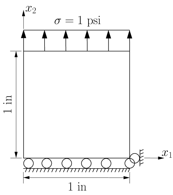
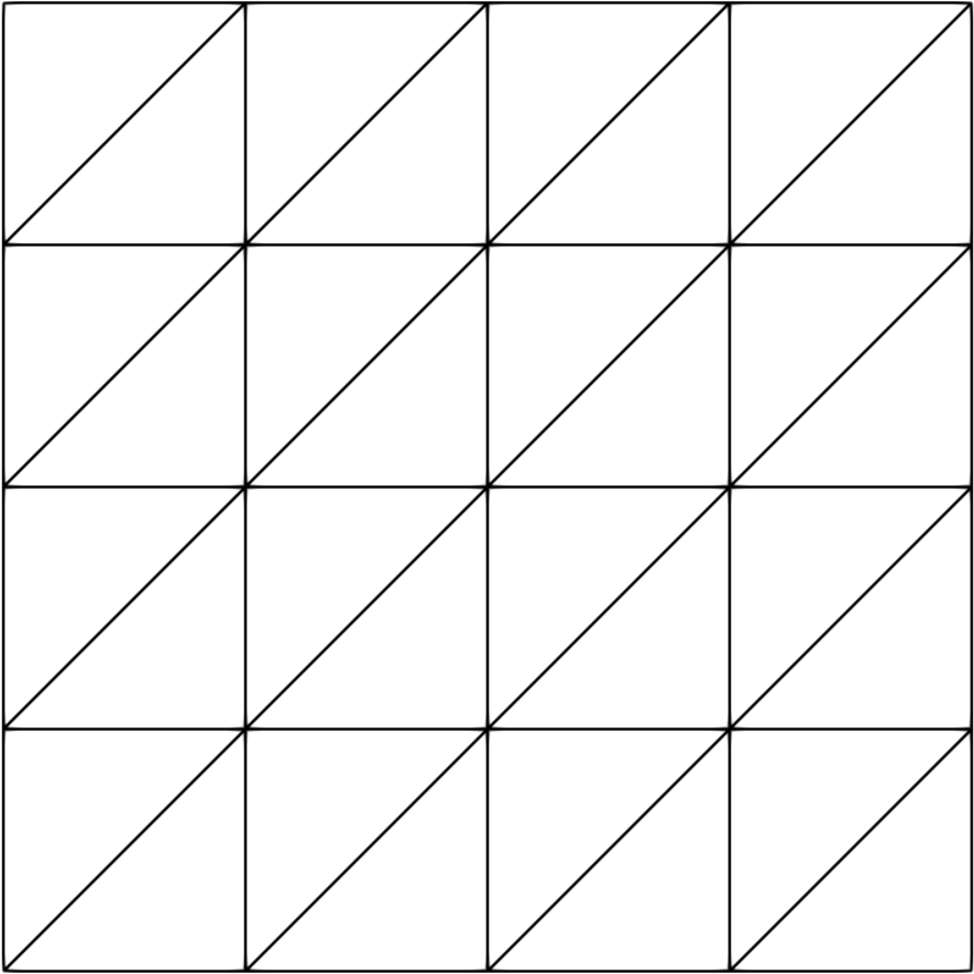
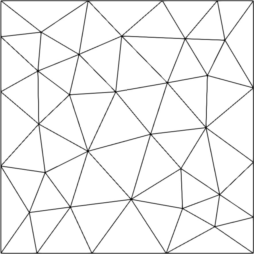
We solve the boundary-value problem (5) for the patch test that is schematically depicted in Figure 5. Plane stress condition is assumed with the following material parameters: $E_{\mathrm{Y}}=3\times 10^{7}$ psi and $\nu=0.3$ . The exact solution for this problem is the linear field $\bm{u}=\left[\begin{array}[]{ccccccccccccccccccccccccccccccccccccccccccccccccccc}\nu(1-x_{1})/E_{\mathrm{Y}}&x_{2}/E_{\mathrm{Y}}\\ \end{array}\right]^{\mathsf{T}}$ . The Dirichlet boundary conditions are imposed as follows: on the bottom boundary, the vertical displacement is fixed, and at its right corner, the displacement is additionally fixed in the horizontal direction. The Neumann boundary conditions are $\bar{\bm{t}}=\left[\begin{array}[]{ccccccccccccccccccccccccccccccccccccccccccccccccccc}0&0\\ \end{array}\right]^{\mathsf{T}}$ on the left and right boundaries, and $\bar{\bm{t}}=\left[\begin{array}[]{ccccccccccccccccccccccccccccccccccccccccccccccccccc}0&\sigma\\ \end{array}\right]^{\mathsf{T}}$ on the top boundary. The Gaussian prior weight function is used for the maximum-entropy basis functions. The background meshes used in this study are depicted in Figure 6. Numerical results for the relative error in the $L^{2}$ norm and the $H^{1}$ seminorm are presented in Tables 1 and 2, respectively, for the MEM and NIVED approaches. Numerical results confirm that the patch test is met to machine precision only for the NIVED method.

Table 1: Relative error in the

L^{2}

norm for the patch test.

Method	Gauss rule	Regular	Distorted	Unstructured
MEM	1-pt (interior of the cell)	$1.0\times 10^{-2}$	$2.0\times 10^{-2}$	$1.7\times 10^{-2}$
MEM	3-pt (interior of the cell)	$2.3\times 10^{-3}$	$1.6\times 10^{-3}$	$1.6\times 10^{-3}$
MEM	6-pt (interior of the cell)	$5.0\times 10^{-5}$	$8.0\times 10^{-4}$	$1.2\times 10^{-3}$
MEM	12-pt (interior of the cell)	$2.2\times 10^{-7}$	$3.0\times 10^{-4}$	$5.0\times 10^{-4}$
NIVED	1-pt (per edge of the cell)	$3.6\times 10^{-15}$	$4.1\times 10^{-15}$	$2.5\times 10^{-15}$

Table 2: Relative error in the

H^{1}

seminorm for the patch test.

Method	Gauss rule	Regular	Distorted	Unstructured
MEM	1-pt (interior of the cell)	$1.4\times 10^{-2}$	$5.4\times 10^{-2}$	$2.5\times 10^{-2}$
MEM	3-pt (interior of the cell)	$2.6\times 10^{-3}$	$5.3\times 10^{-3}$	$4.8\times 10^{-3}$
MEM	6-pt (interior of the cell)	$5.4\times 10^{-5}$	$1.9\times 10^{-3}$	$1.3\times 10^{-3}$
MEM	12-pt (interior of the cell)	$2.3\times 10^{-7}$	$7.7\times 10^{-4}$	$4.5\times 10^{-4}$
NIVED	1-pt (per edge of the cell)	$3.6\times 10^{-15}$	$5.2\times 10^{-15}$	$7.8\times 10^{-15}$

7.2 Numerical stability

To assess the stability of the NIVED method, eigenvalue analyses are performed on a unit square domain. As a reference for comparison, we include the MEM approach in the analyses. The quartic polynomials and the Gaussian radial basis function are considered as the prior weight function in the evaluation of the maximum-entropy basis functions in these analyses. Three zero eigenvalues, which correspond to the three zero-energy rigid-body modes, are obtained for both methods. The three mode shapes that follow the three rigid-body modes are depicted in Figure 7 for the MEM and NIVED methods using the quartic polynomials as the prior weight function. For the quartic prior, instabilities are observed for the MEM with a 1-point Gauss rule since it exhibits nonsmooth mode shapes (Figures 7–7) and even a 12-point Gauss rule is not sufficient for removing the instabilities (Figures 7–7). In stark contrast, Figures 7–7 show the smooth mode shapes that are obtained in the NIVED approach when using the quartic prior.

Similarly, the three mode shapes that follow the three rigid-body modes are depicted in Figure 8 for the MEM and NIVED methods using the Gaussian radial basis function as the prior weight function. For the Gaussian prior, instabilities are observed for the MEM with a 1-point Gauss rule since it exhibits nonsmooth mode shapes (Figures 8–8), but a 6-point Gauss rule can effectively remove the instabilities (Figures 8–8). The NIVED approach using the Gaussian prior is also free of instabilities as revealed by the smooth mode shapes depicted in Figures 8–8.

7.3 Cantilever beam

We conduct a convergence study for the problem of a cantilever beam of unit thickness subjected to a parabolic end load $P=-1000$ lbf. A schematic representation of the problem is shown in Figure 9. Plane strain condition is assumed with material parameters given by $E_{\mathrm{Y}}=10^{7}$ psi and $\nu=0.3$ . The essential boundary conditions on the clamped edge are applied according to the analytical solution given by Timoshenko and Goodier [38]:

\bm{u}=\left[\begin{array}[]{c}-\frac{Px_{2}}{6\bar{E}_{\mathrm{Y}}I}\left((6L-3x_{1})x_{1}+(2+\bar{\nu})x_{2}^{2}-\frac{3D^{2}}{2}(1+\bar{\nu})\right)\\ \frac{P}{6\bar{E}_{\mathrm{Y}}I}\left(3\bar{\nu}x_{2}^{2}(L-x_{1})+(3L-x_{1})x_{1}^{2}\right)\end{array}\right],

where $\bar{E}_{\mathrm{Y}}=E_{\mathrm{Y}}/\left(1-\nu^{2}\right)$ and $\bar{\nu}=\nu/\left(1-\nu\right)$ ; $L=8$ inch is the length of the beam, $D=4$ inch is the height of the beam, and $I=D^{3}/12$ is the second-area moment of the beam section. The exact stress field is:

\left[\begin{array}[]{c}\sigma_{11}\\ \sigma_{22}\\ \sigma_{12}\end{array}\right]=\left[\begin{array}[]{c}\frac{-P(L-x_{1})x_{2}}{I}\\ 0\\ \frac{P}{2I}\left(\frac{D^{2}}{4}-x_{2}^{2}\right)\end{array}\right].

The Neumann boundary conditions are applied using the exact stress field, which gives $\bar{\bm{t}}=\left[\begin{array}[]{ccccccccccccccccccccccccccccccccccccccccccccccccccc}0&0\\ \end{array}\right]^{\mathsf{T}}$ on the top and bottom boundaries, and $\bar{\bm{t}}=\left[\begin{array}[]{ccccccccccccccccccccccccccccccccccccccccccccccccccc}0&\sigma_{12}\\ \end{array}\right]^{\mathsf{T}}$ on the right boundary. For the evaluation of the maximum-entropy basis functions, the Gaussian prior is used. The sequence of background integration meshes used in the study are shown in Figure 10.

The convergence of the MEM and NIVED methods in the $L^{2}$ norm and the $H^{1}$ seminorm of the error are shown in Figure 11. The MEM approach needs a 3-point Gauss rule to deliver the optimal rate in the $L^{2}$ norm. Regarding the $H^{1}$ seminorm, the convergence of the MEM method behaves erratically for 1-point and 3-point Gauss rules due to integration errors, and a 6-point Gauss rule is needed to recover the optimal rate. In contrast, the proposed NIVED method delivers the optimal rate of convergence in both the $L^{2}$ norm and the $H^{1}$ seminorm of the error.

7.4 Infinite plate with a circular hole

The rates of convergence are studied for the problem of an infinite plate with a circular hole that is loaded at infinity according to the tractions $\sigma_{11}=T$ and $\sigma_{22}=\sigma_{12}=0$ (Figure 12). Due to the symmetry of the geometry and boundary conditions, we consider the domain of analysis shown in Figure 12. Plane stress condition is assumed with $E_{\mathrm{Y}}=10^{3}$ psi and $\nu=0.3$ . The exact solution on the domain of analysis is given by [38]

\bm{u}=\left[\begin{array}[]{c}\frac{T}{4G}\bigg(\frac{\kappa+1}{2}r\cos{\theta}+\frac{r_{0}^{2}}{r}\Big((\kappa+1)\cos{\theta}+\cos{3\theta}\Big)-\frac{r_{0}^{4}}{r^{3}}\cos{3\theta}\bigg)\\ \frac{T}{4G}\bigg(\frac{\kappa-3}{2}r\sin{\theta}+\frac{r_{0}^{2}}{r}\Big((\kappa-1)\sin{\theta}+\sin{3\theta}\Big)-\frac{r_{0}^{4}}{r^{3}}\sin{3\theta}\bigg)\end{array}\right],

where $G=E_{\mathrm{Y}}/(2(1+\nu))$ and $\kappa=(3-\nu)/(1+\nu)$ . The exact stress field is:

\left[\begin{array}[]{c}\sigma_{11}\\ \sigma_{22}\\ \sigma_{12}\end{array}\right]=\left[\begin{array}[]{c}T\bigg(1-\frac{r_{0}^{2}}{r^{2}}\left(\frac{3}{2}\cos{2\theta}+\cos{4\theta}\right)+\frac{3r_{0}^{4}}{2r^{4}}\cos{4\theta}\bigg)\\ -T\bigg(\frac{r_{0}^{2}}{r^{2}}\left(\frac{1}{2}\cos{2\theta}-\cos{4\theta}\right)+\frac{3r_{0}^{4}}{2r^{4}}\cos{4\theta}\bigg)\\ -T\bigg(\frac{r_{0}^{2}}{r^{2}}\left(\frac{1}{2}\sin{2\theta}+\sin{4\theta}\right)-\frac{3r_{0}^{4}}{2r^{4}}\sin{4\theta}\bigg)\end{array}\right],

where $r$ is the radial distance from the center $(x_{1}=0,x_{2}=0)$ to a point $(x_{1},x_{2})$ in the domain of analysis. In the computations, the following data are used: $T=100$ psi, $r_{0}=1$ inch and $a=5$ inch. The Dirichlet boundary conditions on the domain of analysis are imposed as follows: $\bar{u}_{1}=0$ on the left side and $\bar{u}_{2}=0$ on the bottom side. The Neumann boundary conditions are prescribed using the exact stresses, as follows: $\bar{\bm{t}}=\left[\begin{array}[]{ccccccccccccccccccccccccccccccccccccccccccccccccccc}\sigma_{12}&\sigma_{22}\\ \end{array}\right]^{\mathsf{T}}$ on the top side and $\bar{\bm{t}}=\left[\begin{array}[]{ccccccccccccccccccccccccccccccccccccccccccccccccccc}\sigma_{11}&\sigma_{12}\\ \end{array}\right]^{\mathsf{T}}$ on the right side. The sequence of background integration meshes used in the study are shown in Figure 13. The Gaussian prior is used for the evaluation of the maximum-entropy basis functions.

The convergence rates that are delivered by the MEM and NIVED approaches in the $L^{2}$ norm and the $H^{1}$ seminorm of the error are compared in Figure 14. We observe that the convergence of the MEM using a 1-point Gauss rule behaves erratically in the $L^{2}$ norm and that the optimal rate of 2 is recovered using a 3-point Gauss rule. Regarding its convergence in the $H^{1}$ seminorm, we observe that it is optimal when using at least a 6-point Gauss rule. On the other hand, the NIVED approach delivers the optimal rates of 2 and 1 in the $L^{2}$ norm and the $H^{1}$ seminorm, respectively.

7.5 $L$ -shaped domain under traction load

An $L$ -shaped domain under traction load is considered. The geometry and boundary conditions are shown in Figure 15, where $H=100$ inch and $p=1$ psi. The thickness is 1 inch. A stress singularity occurs at the re-entrant corner and the exact solution is not known. However, an estimation of the exact strain energy using Richardson’s extrapolation is known and has the value 15566.46 [39]. We use this value to assess the convergence of the strain energy. Plane stress condition is assumed with $E_{\mathrm{Y}}=1$ psi and $\nu=0.3$ . The sequence of background meshes used in this study are depicted in Figure 16. The convergence of the strain energy for the MEM with several Gauss integration rules and for the NIVED approach is shown in Figure 17. We observe that even with a 12-point Gauss rule, the MEM does not uniformly approach the reference value of the strain energy. In contrast, the proposed NIVED scheme uniformly approaches this reference value.

7.6 Manufactured elastostatic problem

In this example, the manufactured elastostatic problem found in Reference [15] is used to assess the performance of the NIVED method. The analysis is conducted on a $2\times 2$ square domain. Plane stress condition is considered with $E_{\mathrm{Y}}=10^{5}$ psi and $\nu=0.3$ . The entire domain boundary is prescribed with the following Dirichlet boundary conditions:

u_{1}(\bm{x})=\sin{x_{1}}\cos{x_{2}},\quad u_{2}(\bm{x})=e^{x_{1}}e^{x_{2}},

which correspond to the exact solutions of the linear elastostatic problem (5) manufactured with a body force given by

\bm{b}=\left[\begin{array}[]{c}(\sin{x_{1}}\cos{x_{2}})\bm{D}(1,1)-(e^{x_{1}}e^{x_{2}})\bm{D}(1,2)-(e^{x_{1}}e^{x_{2}}-\sin{x_{1}}\cos{x_{2}})\bm{D}(3,3)\\ (\cos{x_{1}}\sin{x_{2}})\bm{D}(2,1)-(e^{x_{1}}e^{x_{2}})\bm{D}(2,2)-(e^{x_{1}}e^{x_{2}}-\cos{x_{1}}\sin{x_{2}})\bm{D}(3,3)\end{array}\right].

The exact stress field is

\left[\begin{array}[]{c}\sigma_{11}\\ \sigma_{22}\\ \sigma_{12}\end{array}\right]=\left[\begin{array}[]{c}\bm{D}(1,1)\cos{x_{1}}\cos{x_{2}}+\bm{D}(1,2)e^{x_{1}}e^{x_{2}}\\ \bm{D}(2,1)\cos{x_{1}}\cos{x_{2}}+\bm{D}(2,2)e^{x_{1}}e^{x_{2}}\\ \bm{D}(3,3)(e^{x_{1}}e^{x_{2}}-\sin{x_{1}}\sin{x_{2}}).\end{array}\right].

Figure 18 depicts the background integration meshes used in the study. The Gaussian prior is used for the evaluation of the maximum-entropy basis functions.

The convergence in the $L^{2}$ norm and the $H^{1}$ seminorm for the MEM and NIVED methods are compared in Figure 19. The $L^{2}$ norm is not convergent for the MEM approach using a 1-point Gauss rule, but the optimal rate of 2 is recovered using a 3-point Gauss rule. The convergence of the MEM method in the $H^{1}$ seminorm is not good for 1-, 3- and 6-point Gauss rules, but the optimal rate of 1 is recovered when using a 12-point Gauss rule. The plots show that the NIVED approach delivers the optimal rates of 2 and 1 in the $L^{2}$ norm and the $H^{1}$ seminorm, respectively.

The computational cost of the MEM and NIVED methods are compared in Figure 20. The methods are assessed in terms of accuracy and cell refinement using the normalized CPU time, which is defined as the ratio of the CPU time of a particular model analyzed to the maximum CPU time of any of the models analyzed. In terms of accuracy, we observe that the computational cost of the NIVED scheme is similar to the computational cost of the MEM method with 12-point Gauss rule (Figure 20). This occurs because for a given level of accuracy, the MEM requires a coarser mesh than the NIVED scheme, as shown in Figure 19. In terms of cell refinement, we observe that the computational cost of the NIVED method is similar to the computational cost of the MEM method with a 3-point Gauss rule (Figure 20). However, the MEM with a 3-point Gauss rule does not converge in the $H^{1}$ seminorm, which means that the computational cost of a convergent MEM approach is greater than the computational cost of the NIVED method. In fact, from Figure 19 we know that a 12-point Gauss rule is needed for optimal $H^{1}$ -convergence of the MEM method, but this rule is the most expensive as shown in Figure 20. Combining both the cost in terms of accuracy and cell refinement, we conclude that in general the NIVED scheme can be expected to be faster but less accurate than a convergent MEM approach with the same number of degrees of freedom.

7.7 Manufactured elastodynamic problem

A manufactured elastodynamic problem that is found in Reference [40] is considered. The domain of analysis is a $2\times 2$ square domain and the background meshes considered are the same used for the manufactured elastostatic problem (Figure 18). The material parameters are $E_{\mathrm{Y}}=1\times 10^{5}$ psi, $\nu=0.3$ and $\rho=800$ lb/ $\mathrm{in}^{3}$ , and plane stress condition is assumed. The Gaussian prior is used for the evaluation of the maximum-entropy basis functions.

The problem is manufactured with the following body force:

\bm{b}=\left[\begin{array}[]{c}x_{1}\Big[-2E_{\mathrm{Y}}g(t)+\rho\ddot{g}(t)\left[-(1+\nu)L^{2}+\nu x_{2}^{2}+\frac{1}{3}x_{1}^{2}\right]\Big]\\ x_{2}\Big[2E_{\mathrm{Y}}g(t)+\rho\ddot{g}(t)\left[(1+\nu)L^{2}-\nu x_{1}^{2}-\frac{1}{3}x_{2}^{2}\right]\Big]\end{array}\right],

where $L$ is the side length of the domain of analysis and

g(t)=\alpha\Big[1-e^{-\frac{\beta t^{2}}{2}}\Big].

The exact displacement field solution is

\bm{u}=\left[\begin{array}[]{c}x_{1}g(t)\left[-(1+\nu)L^{2}+\nu x_{2}^{2}+\frac{1}{3}x_{1}^{2}\right]\\ x_{2}g(t)\left[(1+\nu)L^{2}-\nu x_{1}^{2}-\frac{1}{3}x_{2}^{2}\right]\end{array}\right],

and the exact stress field is

\left[\begin{array}[]{c}\sigma_{11}\\ \sigma_{22}\\ \sigma_{12}\end{array}\right]=\left[\begin{array}[]{c}E_{\mathrm{Y}}g(t)\left[x_{1}^{2}-L^{2}\right]\\ E_{\mathrm{Y}}g(t)\left[L^{2}-x_{2}^{2}\right]\\ 0\end{array}\right].

At the initial condition $t=0$ seconds, the body is at rest. The exact displacement field solution is used to impose the Dirichlet boundary conditions along the entire boundary of the domain. The following values for the parameters are used in the computations: $\alpha=0.001$ , $\beta=0.001$ . The Newmark’s constant average acceleration method with a time increment $\Delta t=0.01$ seconds is used as the time integration algorithm.

The convergence of the MEM and NIVED methods in the $L^{2}$ norm and the $H^{1}$ seminorm after 100 time steps (i.e., $t=1$ s) are compared in Figure 21. The MEM approach exhibits suboptimal convergence in the $L^{2}$ norm with a 1-point Gauss rule, but the optimal rate of 2 is recovered using a 3-point Gauss rule. Its convergence in the $H^{1}$ seminorm is optimal when using at least a 12-point Gauss rule. The optimal rates of 2 and 1 are obtained in the $L^{2}$ norm and the $H^{1}$ seminorm, respectively, for the NIVED method.

Similar to the static case, Figure 22 (also obtained at $t=1$ s) reveals that in terms of cell refinement, the computational cost of a convergent MEM approach is greater than the NIVED counterpart thereby making the NIVED approach superior in performance. Moreover, in the dynamic regime the outperformance of the NIVED over the MEM, in terms of cell refinement, is more pronounced as the computational cost of the NIVED approach is about the same as the computational cost of the MEM using a 1-point Gauss rule (Figure 22).

7.8 Thick-walled viscoelastic cylinder subjected to internal pressure

We conclude this section with a demonstration of the nonlinear NIVED formulation for small-displacement and small-strain analysis. The test problem consists of a thick-walled cylinder subjected to internal pressure whose material constitution is a linear isotropic solid described by the Generalized Maxwell viscoelastic model considered in Section 6. This example has been used to assess the virtual element method for inelastic analysis in Reference [37]. Due to symmetry, only a quarter of the cross section of the cylinder is considered, as shown in Figure 23, where $r_{i}=2$ inch, $r_{0}=4$ inch and $p=10$ psi. The material parameters are set to $E=1000$ psi, $\nu=0.3$ and $\lambda_{1}=1$ . The pressure is applied suddenly and the structural response is computed through 20 unit time steps.

In the first part of this study, the convergence of the radial displacement at control points $A$ and $B$ (Figure 23) is assessed. For comparison purposes, the numerical solution obtained with a highly refined mesh of 9-node FEM quadrilateral elements (FEM-Q9) is used. Three sets of choices are considered for the material parameters $\mu_{0}$ and $\mu_{1}$ : $(\mu_{0},\mu_{1})=\{(0.7,0.3),\,(0.3,0.7),\,(0.01,0.99)\}$ . Using $E$ and $\nu$ to calculate the material’s bulk modulus $K$ and (65) to calculate $G(t=20)$ , the effective Poisson’s ratio is calculated as $\nu_{\mathrm{eff}}=\frac{3K-2G(20)}{2(3K+G(20))}$ . For the three preceding sets of parameters this gives at time $t=20$ the values $\nu_{\mathrm{eff}}=\{0.3542,\,0.4338,\,0.4977\}$ , respectively. Thus, for the last set, the material is near-incompressible.

The convergence of the NIVED radial displacement at control points $A$ and $B$ is summarized in Table 3 for the sequence of background integration meshes depicted in Figure 24. Good agreement with the FEM-Q9 reference solution is observed for the three sets of material parameters.

Table 3: NIVED radial displacements at points

A

and

B

for the thick-walled viscoelastic cylinder problem at time

t=20

$(\mu_{0},\mu_{1})=$		$(0.7,0.3)$		$(0.3,0.7)$		$(0.01,0.99)$
mesh	# dofs	$u_{A}$	$u_{B}$	$u_{A}$	$u_{B}$	$u_{A}$	$u_{B}$
Figure 24	882	0.053012	0.031904	0.118830	0.065142	0.646690	0.330050
Figure 24	1922	0.053077	0.031950	0.118970	0.065219	0.647820	0.330170
Figure 24	3362	0.053101	0.031966	0.119020	0.065246	0.648160	0.330210
Figure 24	7442	0.053118	0.031977	0.119050	0.065264	0.648370	0.330240
Figure 24	26082	0.053131	0.031983	0.119070	0.065272	0.648440	0.330210
Ref. (FEM-Q9)	79242	0.053584	0.032425	0.119970	0.066177	0.652880	0.334810

Curves depicting the time history of the radial displacement measured at control points $A$ and $B$ are shown in Figure 25 for the three sets of material parameters. The response curves for the NIVED scheme is plotted for the mesh shown in Figure 24. Good agreement with the FEM-Q9 reference solutions is observed.

Lastly, the performance of the NIVED method for near-incompressible material behavior is studied. The NIVED approach is tested on the background mesh shown in Figure 26 and its radial stress field solution is compared with the corresponding FEM-Q9 solution on the mesh shown in Figure 26. Also on this mesh, the radial stress field is computed with 4-node FEM quadrilateral elements (FEM-Q4). The comparisons are summarized in Figure 27. The radial stress field corresponding to the compressible case $(\mu_{0},\mu_{1})=(0.7,0.3)$ ( $\nu_{\mathrm{eff}}=0.3542$ ) is shown in Figures 27–27 for FEM-Q4, FEM-Q9 and NIVED methods, respectively. It is observed that the three methods perform well in this case. Of course, because of its higher approximation order, the FEM-Q9 radial stress field is smoother than the FEM-Q4 and NIVED radial stress fields.

The radial stress field corresponding to the near-incompressible case $(\mu_{0},\mu_{1})=(0.01,0.99)$ ( $\nu_{\mathrm{eff}}=0.4977$ ) is depicted in Figures 27–27 for FEM-Q4, FEM-Q9 and NIVED methods, respectively. In this case, the FEM-Q9 radial stress field looks smooth and no sign of locking is observed. However, locking behavior is exhibited in the FEM-Q4 case as evidenced by the oscillatory radial stress field. The NIVED scheme performs better than the FEM-Q4 in the incompressible limit, but some small oscillations do occur in the radial stress field and thus it is not completely free of locking. This is not surprising since use of the virtual element framework in the NIVED approach ensures consistency (patch test satisfaction) and stability for a displacement-based formulation. To render the NIVED scheme locking-free in the near-incompressible limit would require introducing, for instance, a form of a nodal averaging technique [41, 42].

8 CONCLUDING REMARKS

In this paper, we proposed a novel nodal integration scheme for meshfree Galerkin methods that is devised from the virtual element decomposition [4], wherein the bilinear form is decomposed into a consistency part and a stability part that ensure that the method is consistent and stable. Linear maximum-entropy meshfree basis functions were adopted, but the formulation is applicable to any other linear meshfree approximant. We referred to this new nodal integration scheme as NIVED. As in any nodal integration method, a nodal representative cell is needed in the NIVED approach. The nodal cell can be constructed from a Voronoi diagram or a Delaunay triangulation by connecting the centroids of triangles surrounding a node.

Numerical tests in linear elastostatic and linear elastodynamic boundary-value problems were conducted, where the focus was on comparing the performance of the NIVED method and the maximum-entropy meshfree method (MEM) using standard Gauss integration. We also provided the extension of the NIVED approach to nonlinear analysis where the material constitution is a linear isotropic solid described by the Generalized Maxwell viscoelastic model. Comparisons with reference solutions obtained with 4-node and 9-node FEM quadrilateral elements were conducted. In the NIVED approach, the weak form integrals are integrated by sampling them at the nodes and the integration at a node is performed using a 1-point Gauss rule over the edges of its nodal representative cell. This task only involves the evaluation of basis functions (no derivatives are needed). In the MEM approach, the integration of the weak form integrals is performed using standard Gauss integration on the interior of triangular cells, which requires the evaluation of basis functions derivatives.

Our main findings from this work are as follows. The NIVED scheme passes the patch test to machine precision, whereas the MEM does not achieve this level of accuracy due to integration errors. The numerical stability test showed that both the NIVED and MEM methods deliver the three zero-energy rigid-body modes, but instability is exhibited only by the MEM method as evidenced by the presence of the nonsmooth eigenmodes that follow the three rigid-body modes. Convergence was assessed through several numerical experiments, which included a cantilever beam subjected to a parabolic end load, an infinite plate with a circular hole and manufactured (elastostatic and elastodynamic) problems. The convergence studies revealed that the NIVED method delivers the optimal rate of convergence in the $L^{2}$ norm and the $H^{1}$ seminorm. On the other hand, the convergence of the MEM was dependent on the number of Gauss points used inside the triangular integration cell. In the tests that were conducted, the MEM required a 3-point Gauss rule for optimal convergence in the $L^{2}$ norm and, depending on the problem, a 6-point or a 12-point Gauss rule for optimal convergence in the $H^{1}$ seminorm. In terms of computational cost, it was shown that for the same number of degrees of freedom the proposed NIVED scheme is faster but less accurate than a convergent MEM approach. We also tested the NIVED and MEM methods in an $L$ -shaped domain under traction load, where the presence of a re-entrant corner introduces a stress singularity that results in a nonsmooth solution. In this case, a study to assess the convergence to a reference value of the strain energy was conducted. The results showed that only the NIVED scheme uniformly approaches the reference strain energy. The performance of the nonlinear NIVED formulation was assessed by solving the problem of a thick-walled viscoelastic cylinder subjected to internal pressure. The radial displacement solution was found to be in good agreement with a reference solution obtained using quadratic (9-node) quadrilateral finite elements. We also showed that for a near-incompressible viscoelastic material, the NIVED scheme is not completely devoid of locking.

In closing, we mention that a desirable feature that can be offered by the (nodally integrated) NIVED approach is that state variables such as strains, stresses and other internal variables in nonlinear computations can be stored at the nodes, which is attractive for Lagrangian large deformation meshfree simulations. This extension of the NIVED method to large deformations is appealing, and is planned as part of future work.

ACKNOWLEDGEMENTS

RSV and AOB acknowledge the support provided by the Chilean National Fund for Scientific and Technological Development (FONDECYT) through grant CONICYT/FONDECYT No. 1181192. NS acknowledges the research support of Sandia National Laboratories. EA gratefully acknowledges the partial financial support of the University of Rome Tor Vergata Mission Sustainability Programme through project SPY-E81I18000540005; and the partial financial support of PRIN 2017 project “3D PRINTING: A BRIDGE TO THE FUTURE (3DP_Future). Computational methods, innovative applications, experimental validations of new materials and technologies,” grant 2017L7X3CS_004. NHK is grateful for the support provided by the Chilean National Fund for Scientific and Technological Development (FONDECYT) through grant CONICYT/FONDECYT No. 1181506.

REFERENCES

[1] T. Belytschko, Y. Y. Lu, and L. Gu. Element-free Galerkin methods. International Journal for Numerical Methods in Engineering, 37(2):229–256, 1994.
[2] B. Li, F. Habbal, and M. Ortiz. Optimal transportation meshfree approximation schemes for fluid and plastic flows. International Journal for Numerical Methods in Engineering, 83(12):1541–1579, 2010.
[3] D. Sulsky, Z. Chen, and H. L. Schreyer. A particle method for history-dependent materials. Computer Methods in Applied Mechanics and Engineering, 118(1):179–196, 1994.
[4] L. Beirão da Veiga, F. Brezzi, A. Cangiani, G. Manzini, L. D. Marini, and A. Russo. Basic principles of virtual element methods. Mathematical Models and Methods in Applied Sciences, 23(1):199–214, 2013.
[5] A. Ortiz-Bernardin, A. Russo, and N. Sukumar. Consistent and stable meshfree Galerkin methods using the virtual element decomposition. International Journal for Numerical Methods in Engineering, 112(7):655–684, 2017.
[6] J. Dolbow and T. Belytschko. Numerical integration of Galerkin weak form in meshfree methods. Computational Mechanics, 23(3):219–230, 1999.
[7] S. N. Atluri, H. G. Kim, and J. Y. Cho. A critical assessment of the truly Meshless Local Petrov-Galerkin (MLPG), and Local Boundary Integral equation (LBIE) methods. Computational Mechanics, 24(5):348–372, 1999.
[8] S. De and K. J. Bathe. The method of finite spheres with improved numerical integration. Computers and Structures, 79(22–25):2183–2196, 2001.
[9] S. Beissel and T. Belytschko. Nodal integration of the element-free Galerkin method. Computer Methods in Applied Mechanics and Engineering, 139(1):49–74, 1996.
[10] J.-S. Chen, C. T. Wu, S. Yoon, and Y. You. A stabilized conforming nodal integration for Galerkin mesh-free methods. International Journal for Numerical Methods in Engineering, 50(2):435–466, 2001.
[11] J.-S. Chen, S. Yoon, and C. T. Wu. Non-linear version of stabilized conforming nodal integration for Galerkin mesh-free methods. International Journal for Numerical Methods in Engineering, 53(12):2587–2615, 2002.
[12] M. A. Puso, J.-S. Chen, E. Zywicz, and W. Elmer. Meshfree and finite element nodal integration methods. International Journal for Numerical Methods in Engineering, 74(3):416–446, 2008.
[13] J.-S. Chen, M. Hillman, and M. Rüter. An arbitrary order variationally consistent integration for Galerkin meshfree methods. International Journal for Numerical Methods in Engineering, 95(5):387–418, 2013.
[14] Q. Duan, X. Li, H. Zhang, and T. Belytschko. Second-order accurate derivatives and integration schemes for meshfree methods. International Journal for Numerical Methods in Engineering, 92(4):399–424, 2012.
[15] Q. Duan, X. Gao, B. Wang, , X. Li, H. Zhang, T. Belytschko, and Y. Shao. Consistent element-free Galerkin method. International Journal for Numerical Methods in Engineering, 99(2):79–101, 2014.
[16] Q. Duan, X. Gao, B. Wang, X. Li, and H. Zhang. A four-point integration scheme with quadratic exactness for three-dimensional element-free Galerkin method based on variationally consistent formulation. Computer Methods in Applied Mechanics and Engineering, 280:84–116, 2014.
[17] G. R. Liu, K. Y. Dai, and T. T. Nguyen. A smoothed finite element method for mechanics problems. Computational Mechanics, 39(6):859–877, 2007.
[18] C. T. Dyka, P. W. Randles, and R. P. Ingel. Stress points for tension instability in SPH. International Journal for Numerical Methods in Engineering, 40(13):2325–2341, 1997.
[19] M. Hillman and J.-S. Chen. An accelerated, convergent, and stable nodal integration in Galerkin meshfree methods for linear and nonlinear mechanics. International Journal for Numerical Methods in Engineering, 107(7):603–630, 2016.
[20] L. Beirão da Veiga, F. Brezzi, and L. D. Marini. Virtual elements for linear elasticity problems. SIAM Journal on Numerical Analysis, 51(2):794–812, 2013.
[21] C. Talischi and G. H. Paulino. Addressing integration error for polygonal finite elements through polynomial projections: A patch test connection. Mathematical Models and Methods in Applied Sciences, 24(08):1701–1727, 2014.
[22] A. L. Gain, C. Talischi, and G. H. Paulino. On the virtual element method for three-dimensional linear elasticity problems on arbitrary polyhedral meshes. Computer Methods in Applied Mechanics and Engineering, 282(0):132–160, 2014.
[23] G. Manzini, A. Russo, and N. Sukumar. New perspectives on polygonal and polyhedral finite element methods. Mathematical Models and Methods in Applied Sciences, 24(08):1665–1699, 2014.
[24] A. Cangiani, G. Manzini, A. Russo, and N. Sukumar. Hourglass stabilization and the virtual element method. International Journal for Numerical Methods in Engineering, 102(3–4):404–436, 2015.
[25] N. Sukumar and R. W. Wright. Overview and construction of meshfree basis functions: from moving least squares to entropy approximants. International Journal for Numerical Methods in Engineering, 70(2):181–205, 2007.
[26] M. Arroyo and M. Ortiz. Local maximum-entropy approximation schemes: a seamless bridge between finite elements and meshfree methods. International Journal for Numerical Methods in Engineering, 65(13):2167–2202, 2006.
[27] L. L. Yaw, N. Sukumar, and S. K. Kunnath. Meshfree co-rotational formulation for two-dimensional continua. International Journal for Numerical Methods in Engineering, 79(8):979–1003, 2009.
[28] L. Beirão da Veiga, F. Brezzi, L. D. Marini, and A. Russo. The Hitchhiker’s Guide to the Virtual Element Method. Mathematical Models and Methods in Applied Sciences, 24(08):1541–1573, 2014.
[29] L. Beirão da Veiga, F. Dassi, and A. Russo. High-order virtual element method on polyhedral meshes. Computers & Mathematics with Applications, 74(5):1110–1122, 2017.
[30] F. Dassi and L. Mascotto. Exploring high-order three dimensional virtual elements: Bases and stabilizations. Computers & Mathematics with Applications, 75(9):3379–3401, 2018.
[31] E. Artioli, L. Beirão da Veiga, C. Lovadina, and E. Sacco. Arbitrary order 2D virtual elements for polygonal meshes: part I, elastic problem. Computational Mechanics, 60(3):355–377, 2017.
[32] B. Ahmad, A. Alsaedi, F. Brezzi, L.D. Marini, and A. Russo. Equivalent projectors for virtual element methods. Computers & Mathematics with Applications, 66(3):376–391, 2013.
[33] G. Vacca and L. Beirão da Veiga. Virtual element methods for parabolic problems on polygonal meshes. Numerical Methods for Partial Differential Equations, 31(6):2110–2134, 2015.
[34] G. Vacca. Virtual element methods for hyperbolic problems on polygonal meshes. Computers & Mathematics with Applications, 74(5):882–898, 2017.
[35] K. Park, H. Chi, and G. H. Paulino. On nonconvex meshes for elastodynamics using virtual element methods with explicit time integration. Computer Methods in Applied Mechanics and Engineering, 356:669–684, 2019.
[36] O. C. Zienkiewicz and R. L. Taylor. The Finite Element Method for Solid and Structural Mechanics. Butterworth-Heinemann, Oxford, UK, sixth edition, 2005.
[37] E. Artioli, L. Beirão da Veiga, C. Lovadina, and E. Sacco. Arbitrary order 2D virtual elements for polygonal meshes: part II, inelastic problem. Computational Mechanics, 60(4):643–657, 2017.
[38] S. P. Timoshenko and J. N. Goodier. Theory of Elasticity. McGraw-Hill, NY, third edition, 1970.
[39] P. Beckers, H.-G. Zhong, and E. Maunder. Numerical comparison of several a posteriori error estimators for 2d stress analysis. Revue Européenne des Éléments Finis, 2(2):155–178, 1993.
[40] Q. Duan, B. Wang, X. Gao, and X. Li. Quadratically consistent nodal integration for second order meshfree Galerkin methods. Computational Mechanics, 54(2):353–368, 2014.
[41] C. R. Dohrmann, M. W. Heinstein, J. Jung, S. W. Key, and W. R. Witkowski. Node-based uniform strain elements for three-node triangular and four-node tetrahedral meshes. International Journal for Numerical Methods in Engineering, 47(9):1549–1568, 2000.
[42] M. A. Puso and J. Solberg. A stabilized nodally integrated tetrahedral. International Journal for Numerical Methods in Engineering, 67(6):841–867, 2006.

		$\displaystyle\|E\|\,\bm{\upvarepsilon}_{E}^{\mathsf{T}}(\bm{v}^{h})\bm{D}_{\mathsf{T}}\|_{n+1}\bm{\upvarepsilon}_{E}(\Delta\bm{u}^{h})+\int_{E}\left[\bm{\upvarepsilon}(\bm{v}^{h})-\bm{\upvarepsilon}_{E}(\bm{v}^{h})\right]^{\mathsf{T}}\bm{D}_{\mathsf{T}}\|_{n+1}\left[\bm{\upvarepsilon}(\Delta\bm{u}^{h})-\bm{\upvarepsilon}_{E}(\Delta\bm{u}^{h})\right]\,d\bm{x}$
		$\displaystyle=-\Big\{\|E\|\,\bm{\upvarepsilon}_{E}^{\mathsf{T}}(\bm{v}^{h})\bm{\upsigma}_{n+1}(\bm{\upvarepsilon}_{E}(\bm{u}_{n+1}^{h}))+\int_{E}\left[\bm{\upvarepsilon}(\bm{v}^{h})-\bm{\upvarepsilon}_{E}(\bm{v}^{h})\right]^{\mathsf{T}}\bm{\upsigma}_{n+1}(\bm{\upvarepsilon}(\bm{u}_{n+1}^{h})-\bm{\upvarepsilon}_{E}(\bm{u}_{n+1}^{h}))\,d\bm{x}\Big.$
		$\displaystyle\Big.\quad\quad\quad-\|E\|\,(P_{0}\bm{v}^{h})^{\mathsf{T}}\bm{b}_{E}-\|S\|\,(P_{0}\bm{v}^{h})^{\mathsf{T}}\bar{\bm{t}}_{S}\Big\},$		(73)

A nodal integration scheme for meshfree Galerkin methods using the virtual element decomposition

Abstract

keywords

1 INTRODUCTION

2 MAXIMUM-ENTROPY BASIS FUNCTIONS

3 GOVERNING EQUATIONS

3.1 Strong form

3.2 Weak form

4 NODAL INTEGRATION USING THE VIRTUAL ELEMENT DECOMPOSITION

4.1 Nodal integration cell

4.2 Nodal contribution

4.3 Virtual element decomposition

4.4 Projection operator

4.5 Projection matrix

4.6 Nodally integrated stiffness matrix

4.7 Nodally integrated force vector

4.8 Nodally integrated mass matrix

5 PATCH TEST SATISFACTION

6 EXTENSION TO NONLINEAR ANALYSIS: THE VISCOELASTIC CASE

7 NUMERICAL EXPERIMENTS

7.1 Patch test

7.2 Numerical stability

7.3 Cantilever beam

7.4 Infinite plate with a circular hole

7.5 LL-shaped domain under traction load

7.6 Manufactured elastostatic problem

7.7 Manufactured elastodynamic problem

7.8 Thick-walled viscoelastic cylinder subjected to internal pressure

8 CONCLUDING REMARKS

ACKNOWLEDGEMENTS

REFERENCES

7.5 $L$ -shaped domain under traction load