Tracking VIX with VIX Futures:
Portfolio Construction and PerformanceThanks: This draft is submitted for the Handbook of Applied Investment Research, edited by W. Ziemba et al., forthcoming, 2019.
Abstract
We study a series of static and dynamic portfolios of VIX futures and their effectiveness to track the VIX index. We derive each portfolio using optimization methods, and evaluate its tracking performance from both empirical and theoretical perspectives. Among our results, we show that static portfolios of different VIX futures fail to track VIX closely. VIX futures simply do not react quickly enough to movements in the spot VIX. In a discrete-time model, we design and implement a dynamic trading strategy that adjusts daily to optimally track VIX. The model is calibrated to historical data and a simulation study is performed to understand the properties exhibited by the strategy. In addition, comparing to the volatility ETN, VXX, we find that our dynamic strategy has a superior tracking performance.
1 Introduction
For all long-term investors it is very important to be able to effectively control the risk exposure of their portfolios through varying market conditions. Downside risk protection is particularly crucial. This motivates investors to consider different instruments and strategies to potentially hedge against market turbulence. One of the most widely recognized measure of expected market volatility is the CBOE Volatility Index (VIX). This is a desirable asset to hold as it has been observed empirically that volatility and market returns are anti-correlated, an effect known as asymmetric volatility.11 1 See Black 1976 for the first use of this term. Therefore, having exposure to VIX would protect the investor by providing some gains to offset market downturns.


To illustrate this, let us consider two portfolios: a portfolio fully invested in the SPDR S&P 500 ETF (SPY), and another portfolio with 90% wealth in SPY and 10% wealth in VIX, assuming that VIX is tradable.22 2 Also discussed in the authors’ companion paper, Leung and Ward 2018. Figure 1(a) corresponds to the period of 2011 when the U.S. suffered a credit rating downgrade by Standard and Poor’s. News of a negative outlook by S&P of the U.S. credit rating broke on April 18th, 2011.33 3 See New York Times article: http://www.nytimes.com/2011/04/19/business/19markets.html. The SPY position would go on to lose about 10% with a volatile trajectory for a few months past the official downgrade on August 5th, 2011.44 4 See http://www.nytimes.com/2011/08/06/business/us-debt-downgraded-by-sp.html. In contrast, a hypothetical portfolio with a 90/10 mix of SPY and VIX would be stable through the downgrade and end up with a positive return. In Figure 1(b), we observe that the same pair of portfolios earned roughly the same 15% return in 2014. However, with SPY alone the portfolio is visibly more volatile than the portfolio with SPY and VIX. The reason is that large drawdowns (for example on October 15th, 2014) were met by rises in VIX, creating a stabilizing effect on the portfolio’s value.
Such a strategy is also beneficial for longer-term investment. If one invests 10% of wealth in VIX and the remaining fraction in SPY on January 30, 2009, then the realized Sharpe ratio of holding this portfolio till December 27, 2017 is 1.16. By comparison, the SPY-only portfolio attains a Sharpe ratio of 1. The improvement is due mostly to a strong reduction in volatility from 16.07% to 12.55% and our calculations show further that investing up to 26% of wealth in VIX, with remainder in SPY, would yield an even higher Sharpe ratio of 1.45.
The benefits of having VIX exposure are obvious, but in reality VIX is not directly tradable. Instead, volatility exposure is achieved through the use of VIX futures or options, and a number of exchange-traded funds/notes (ETF/Ns). The most traded VIX-based ETN is the iPath S&P 500 VIX Short-Term Futures ETN (ticker: VXX). However, as we will discuss, VXX fails to track VIX well and more generally, VIX ETF/Ns bring persistent negative returns. In the literature, a number of studies (Deng et al. 2012; Eraker and Wu 2013; Whaley 2013) have also illustrated the negative returns associated with VIX futures and ETNs such as VXX. Nevertheless, VIX futures are also widely used for speculative trading and managed futures portfolios (Leung et al. 2016; Jiao 2016; Leung and Yan 2018; Leung and Yan 2019. As summarized by Bloomberg on January 29, 2019, “due to a structural quirk, the note lost 99 percent of its value over its life – but it also democratized investor access to implied U.S. equity volatility. ”
In this paper, we discuss the price dynamics of VIX futures and the underlying index, and construct static and dynamic portfolios of VIX futures for the purpose of tracking the index. In addition to deriving and implementing the optimal tracking strategies, our main objective is to examine closely the effectiveness of the tracking portfolios. For a thorough related study by the authors on discrete-time and continuous-time tracking of VIX and other indices involving futures/other derivatives, we refer to Leung and Ward 2015; Leung and Ward 2018; Ward 2017.
Our study is structured as follows. In Section 2, we analyze the empirically observed return dependency of the VIX index and VIX futures. In Section 3, we construct static portfolios of VIX futures for tracking VIX and investigate their tracking effectiveness over a long period of time. Our study illustrates a number of pitfalls in using static futures portfolios to attempt to track VIX, which motivates us to consider a dynamic approach as discussed in Section 4. Assuming a model that captures the mean-reverting dynamics of VIX, we derive the optimal dynamic replicating strategy that is adaptive to the daily fluctuations of VIX. The replicating strategy is implemented in Section 5. Concluding remarks are provided in Section 6.
2 VIX Spot & Futures
We begin by analyzing the price dynamics of the VIX Futures with respect to spot VIX. The historical price data for VIX futures are obtained from Quandl.55 5 Refer to https://www.quandl.com/collections/futures/cboe for documentation on the available CBOE data. One can search for specific contracts at https://www.quandl.com/data/CBOE-Chicago-Board-Options-Exchange. We have validated the Quandl data against that directly from the CBOE.66 6 CBOE publishes the historical data as well here: http://cfe.cboe.com/data/historicaldata.aspx. For the spot VIX data as well as the related ETNs, we use Yahoo! Finance.77 7 Quandl also has spot VIX data available, but it is sourced from Yahoo! Finance and we have validated the two datasets against each other.
After compiling, our dataset consists of the entire closing price history from March , 2004 (the first day VIX futures began trading) through January , 2017. However, we choose to analyze only the period from January , 2011 (first trading date of 2011) through December , 2016, which is a 6-year period from 2011 to 2016. In our opinion, this amount of data is sufficient to avoid overfitting and recent enough to understand the current dynamics among VIX, futures, and VXX. The entire sample period from 2011 to 2016 contains 1,510 total trading days of data. Moreover, on any given day of the sample set there are between 7 and 9 futures contracts available. In particular, there are 15 days with only 7 futures contracts available, 278 days with only 8 futures contracts available and 1,217 days with a full 9 months of contracts available. These contracts are always consecutive months (starting with the 1-month contract) over this time period. In other words, when there are futures contracts available for trading, they always consist of the front months. As an example, if the current trading date were sometime early in January (before the January futures expiry), and 7 futures contracts were available for trading, then the maturities of the futures contracts would be the months of January through July, consecutively. These features of the dataset are consistent with CBOE protocol. They state they will currently list up to 9 near-term months for trading.88 8 See http://cfe.cboe.com/products/spec_vix.aspx. However, in our analysis, we eliminate the eighth and ninth month contract as it is not always the case that one can trade the eighth or ninth month contract. This allows us to use the full 1,510 days of data and avoid the need to eliminate the days with only 7 or 8 futures for trading.
2.1 Return Dependency
We begin with a regression of the 1-day returns of VIX futures against the corresponding 1-day returns of VIX. The results are summarized in Table 1.
| Futures | Slope | Intercept | ||
|---|---|---|---|---|
| 1-month | 0.604 | 3.54 | 0.792 | 0.0242 |
| 2-month | 0.428 | 3.33 | 0.759 | 0.0189 |
| 3-month | 0.321 | 2.45 | 0.718 | 0.0158 |
| 4-month | 0.267 | 1.98 | 0.688 | 0.0141 |
| 5-month | 0.226 | 1.79 | 0.645 | 0.0131 |
| 6-month | 0.200 | 1.62 | 0.615 | 0.0124 |
| 7-month | 0.184 | 1.35 | 0.597 | 0.0118 |
In Table 1, we observe the high values for all futures, suggesting that they are highly correlated with the spot. The futures with shorter maturities have higher values. This can be explained by (i) the fact that futures prices tend to approach the spot price towards maturity, and (ii) that long dated contracts are less liquid than the short term contracts. The slope coefficients are all statistically significant and less than , which is intuitive as futures returns tend to be less volatile than spot returns. The negative intercepts, which are statistically significant, indicate that futures prices tend to fall even if the spot price does not move. The reason lies in the term structure of VIX futures, which is as we will see is typically increasing in time-to-maturity. Even if the spot price does not move, the futures prices tend to decrease to match the spot price towards maturity, contributing to a negative intercept.
In Figure 2, we plot the time series of spot VIX, the 1-month futures price (May-16 contract), and the 7-month futures price (Nov-16 contract) over the period from April , 2016 (1 day after the expiration of the April-16 contract) to May , 2016 (the expiration date of the May-16 contract). Notice that the spot, 1-month futures price and 7-month futures price all tend to move together. However, the moves in the spot are larger than moves in the futures prices. We also observe that the spot and futures prices often move in the same direction, but the futures prices do not move 1 for 1 with the spot. As one might expect, this effect is more pronounced for the 7-month contract, which barely moves over the period. For example, from trading day 4 to 5, we have a large up move in VIX of $1.45 which is only met by an increase of $1.00 by the 1-month contract and an increase of $0.50 by the 7-month contract.

Notice also that there is a slight discrepancy between the 1-month futures price at maturity and spot price. In theory, futures prices should converge to the spot price. However, market frictions, settlement rules99 9 See https://cfe.cboe.com/products/settlement_vix.aspx for VIX derivatives’ settlement procedures. and non-tradability of the spot can substantially limit this convergence, as is seen in other futures markets, e.g. agricultural futures (Guo and Leung 2017). For the non-convergence phenomenon of VIX futures, we refer to Pavlova and Daigler 2008 for an empirical study.


We plot the term structure of VIX futures as observed at several different time points throughout the first 6 months of 2016 (left) and 2009 (right) in Figure 3. The typical case for the VIX market is an increasing and concave futures curve (see left panel). However, in January 2016, VIX spiked as did expectations of future volatility.1010 10 One can find a discussion of trends in volatility in late January 2016 in the following article: https://tickertape.tdameritrade.com/options/2016/01/volatility-high-early-2016-42727. Spikes like this can cause the term structure of VIX futures to invert, yielding a decreasing and convex futures curve. On the right panel of Figure 3, we plot the term structures in early 2009 where futures prices are at very high levels and the term structure shows different shape properties. In the literature, there exist a number of models for VIX dynamics that yield the observed term structures (e.g. increasing concave, or decreasing convex). These include the Cox-Ingersoll-Ross (CIR) model (see Grübichler and Longstaff 1996 and Zhang and Zhu 2006), Ornstein-Uhlenbeck (OU) model and exponential OU model (see Leung and Li 2016), and models with multiple stochastic factors and regimes (see Mencia and Sentana 2013; Jiao 2016).
2.2 Long-Term Dependency
When we conduct regressions of futures returns against spot returns over longer holding periods, new patterns emerge. We use disjoint intervals of various lengths when we compute the returns, meaning that for the longer horizons we have fewer data points, but even for the 30-day horizon we have approximately 50 data points.
In Figure 4, we plot the regressions of 1-month futures returns versus VIX returns for both 1-day returns (left) and 10-day returns (right), plotted on the same - axis scale. The red x’s mark pairs of returns, while the black line is the best fit line. One observes that the 10-day returns are much larger and consequently more volatile than the 1-day returns. However, for both holding periods, the futures returns are less volatile than the corresponding spot returns. To be precise, we find that the 1-day returns of the spot vary between -26.96% and 50%, while for the 10-day returns they vary between -39.76% and 148.06% (i.e. the longer holding period has more volatile returns). On the other hand for the 1-month futures, the 1-day returns vary between -20.81% and 35.83%, while the 10-day returns vary between -36.91% and 88.89% (i.e. futures returns are less volatile than the respective spot returns).


In the plot, the slope is slightly higher for the 10-day returns as compared to the 1-day returns. Moreover, for the 1-day returns the scatter plot is more tightly bound to the best fit line indicating a better fit than observed for the 10-day returns. However, this pattern does not hold in general. There is no discernible pattern in either the values or slope coefficients as the holding period is lengthend. This can be demonstrated by looking at a plot of or slope vs. holding period. We omit such a plot here as there is no clear pattern of increasing or decreasing predictive power (as measured by ) or leverage necessary to replicate the spot returns in the plot for any maturity contract. (Leverage can be measured by the reciprocal of the slope.)
On the other hand, if we fix the holding period and increase the maturity of the contract, we see a decrease in predictive power and a decrease in slope. (Thus, an increase in leverage necessary to replicate the spot.) We demonstrate this for a number of different holding periods (1, 5, 10 and 15 days) in Table 2. In the top half, we give the slope coefficients for the regressions of futures returns against spot returns and in the bottom half, we display the values. By looking across the rows in either half, one notices a decrease in the reported statistic. This reaffirms our earlier observation that the spot is more closely tracked by short-term futures than long term futures. Indeed, over a 15 day period, the results indicate that about 1.6x leverage is required to track the spot with 1-month futures vs. 7.2x leverage for the 7-month futures. These implied leverage values are obtained by computing the reciprocals of the slopes (0.622, and 0.139, respectively). The leverage for the 7-month futures is quite substantial and is likely not be feasible in the marketplace due to trading costs or exchange limits.
| Days | 1-Mon | 2-Mon | 3-Mon | 4-Mon | 5-Mon | 6-Mon | 7-Mon | |
|---|---|---|---|---|---|---|---|---|
| Slope | 1 | 0.604 | 0.428 | 0.321 | 0.267 | 0.226 | 0.200 | 0.184 |
| 5 | 0.668 | 0.471 | 0.358 | 0.291 | 0.244 | 0.219 | 0.199 | |
| 10 | 0.641 | 0.424 | 0.320 | 0.254 | 0.206 | 0.185 | 0.167 | |
| 15 | 0.622 | 0.373 | 0.283 | 0.218 | 0.171 | 0.153 | 0.139 | |
| 1 | 0.792 | 0.759 | 0.718 | 0.688 | 0.645 | 0.615 | 0.597 | |
| 5 | 0.832 | 0.825 | 0.779 | 0.738 | 0.697 | 0.673 | 0.649 | |
| 10 | 0.750 | 0.750 | 0.691 | 0.630 | 0.562 | 0.540 | 0.519 | |
| 15 | 0.663 | 0.639 | 0.574 | 0.488 | 0.395 | 0.376 | 0.352 |
Although not immediately discernible, in Figure 4, the intercept is more negative for the 10-day returns as compared to the 1-day returns. This confirms a property we have already discussed: futures tend to underperform and lose money relative to the spot returns. The more negative intercept indicates that this underperformance worsens over longer horizons. To see this more generally, in Figure 5, we plot the intercepts for the regressions of returns of 1-month futures (black), 3-month futures (red) and 6-month futures (blue) across many different holding periods (from 1 day up to 30 days). It is quite clear that as the holding period is lengthened, the intercept becomes increasingly more negative. All intercepts (as well as the slopes from before) reported here are statistically significant at the 1% significance level. Thus, a statistically significant discrepancy exists and continues to worsen as holding period is lengthened.

3 Static Replication Strategies
In this section, we investigate the static replication of VIX using futures. Portfolios based on two different optimization criteria are considered. In Section 3.1, we consider replication by optimizing the weights of the portfolio to match the physical dollar price of VIX over the training period. Due to the mean-reverting nature of VIX, the optimal portfolio is effectively all cash as this will keep the portfolio roughly near the mean level of VIX through the in-sample period. This motivates optimizing the portfolio to match the returns as closely as possible. The performance is improved upon with this change of criterion, but we demonstrate that it simply is difficult to track VIX with a static portfolio of futures. Unless otherwise noted, the training or in-sample period is the 5-year period from 2011 to 2015, and the test or out-of-sample period is the year 2016.
3.1 Physical Replication by Static Futures Portfolios
In this section, we consider static positions including 1 or more futures contracts. By a static position in the futures contract, we mean a position that is constantly rolled over into the next futures contract. For example, a static investment of in 1-month futures would proceed as follows. First, purchase units of the current 1-month contract and hold it until maturity. The position’s value at that time can be denoted by . Then, one uses this final value to purchase what was previously (e.g. at time 0) the 2-month futures, but is now the 1-month futures. If this futures price is denoted , then one purchases units of the new 1-month contract and hold that contract until maturity. This process is continued indefinitely at each maturity date.
There will be no cash withdrawals/injections at the roll periods (e.g. to keep the number of units of futures constant.) This makes the position completely self-financing, though the number of achievable units of futures will vary over time (i.e. it is completely possible that ). The static position described here, starting on January , 2011 with $100 will be called the value of the 1-month futures contract. One can analogously define the 2-month, 3-month, etc. values as positions that always maintain all money in 2-month, 3-month, etc. contracts.
The portfolio value on day is denoted by and consists of various VIX futures contracts. The value of spot VIX on day is denoted by . The precise weightings amongst the futures will be chosen so as to minimize the sum of squared errors:
| (3.1) |
where is the number of trading days in the in-sample period.
Let be the number of futures contracts being considered and be the real-valued vector of portfolio weights. In particular, represents the weight given to the money market account.1111 11 The money market account yields overnight LIBOR. The data was obtained from the Federal Reserve Bank of St. Louis (FRED); see https://fred.stlouisfed.org/series/USDONTD156N. Next, denote by a matrix containing as columns the historical values of the money market account and the various futures contracts. Finally, denote by a vector containing the historical values of VIX. All prices come from the in-sample set and are normalized to start at $100 on day . With this notation and optimization criterion (3.1), we derive the following constrained least squares optimization problem:
| (3.2) | ||||||
The normalization implies that an investor starting with will invest $ into the th futures contract and $ into the money market account. For simplicity of the subsequent analysis, we consider portfolios containing any of the four of the following contracts: 1-month, 2-month, 6-month and 7-month. Allowing for any number of futures in the portfolio this naturally yields (subtract 1 because we do not look at the portfolio using no futures as that is trivial) different potential portfolios. Using all 7 available futures and their subsets would be untenable and obscure the analysis. The four contracts selected here represent the shortest and longest dated maturities that are available in the VIX futures market on every day of both the in-sample and out-of-sample period.
The resuls of the optimization are given in Table 3. As above, always represents the weight on the money market account. All other are ordered so that if , represents the weight on a nearer term contract than . For example, in row 6 we are considering a portfolio of 1-month and 6-month futures. Thus, is the weight on 1-month futures, while represents the weight on 6-month futures. The Root Mean Squared Error (RMSE) has a standard definition in terms of the SSE defined in Equation (3.1). Precisely,
| (3.3) |
where for the in-sample period and for the out-of-sample period. Our choice of initial capital of $100 allows us to interpret RMSE as the average percentage deviation of the portfolio value from the spot price during the in-sample or out-of-sample period.
The RMSE values are quite large, indicating poor in-sample and out-of-sample tracking performance. To benchmark the performance we can compare the RMSE values to those achieved by VXX. The in-sample RMSE for VXX is 72.05%, while the out-of-sample value is 21.97%. The values indicate the futures based portfolios perform significantly better in-sample than does VXX. Out-of-sample, the futures based portfolios performs only slightly better in a few cases.
Remark 3.1
The difference in performance in-sample vs. out-of-sample for VXX is driven mostly by the difference in length of the two data sets. Recall that VXX is an unlevered portfolio of VIX futures, which we have demonstrated in Section 2 does not react quickly to spot VIX price movements. Thus, once VXX has fallen away from VIX, it cannot return to the dollar value of VIX and additions to SSE continue to accumulate.
Though the performance is somewhat better than VXX, the resulting strategies break with intuition. All portfolios are barely net long in the various futures contracts employed. This is seen prominently in the those with one or two futures only. For example, the 1-month only portfolio invests only 15.2% of wealth in the value of the 1-month futures contract and the remaining 84.8% is held in cash. This is due to the choice of SSE as an optimization criterion and that we measure SSE on the physical dollar price. This combination makes the optimization somewhat forward looking. It considers all at once the values VIX will take over the in-sample period. In particular, VIX is highly mean-reverting and thus, holding the portfolio value at the average level of VIX over the period is the best choice. Futures simply do not track the spot well so it is best to ignore any spikes and remain constant over time.
Finally, in Figure 6 we plot the time series of spot VIX, the ETF VXX, and the optimal (across all combinations of portfolio components) out-of-sample portfolio. As discussed above, the optimal portfolio is relatively flat holding most of its value (91.7%) and is barely net long in 1-month and 6-month futures (8.3%). On the other hand VXX is more reactive to the spot price movements, but quickly diverges from spot VIX. Thereafter it is unable to recover and continues to fall away from spot VIX. By the end of the in-sample period, VXX has fallen to $3.44, and for the out-of-sample period, it has fallen to $29.89. In neither does samples does the optimal portfolio diverge in this manner. It instead stays roughly constant at VIX’s average level over both periods. Neither portfolio appears a perfect surrogate for trading VIX and therefore we consider alternative methods to constructing portfolios of futures to track VIX in the next section.
| Futures | in-RMSE | out-RMSE | |||||
|---|---|---|---|---|---|---|---|
| 1-m | 0.848 | 0.152 | - | - | - | 30.724 | 23.345 |
| 2-m | 0.857 | 0.143 | - | - | - | 31.153 | 26.074 |
| 6-m | 0.811 | 0.189 | - | - | - | 31.026 | 28.840 |
| 7-m | 0.777 | 0.223 | - | - | - | 30.835 | 28.616 |
| 1-m, 2-m | 0.932 | 2.114 | 2.046 | - | - | 27.741 | 19.521 |
| 1-m, 6-m | 0.917 | 0.345 | 0.262 | - | - | 30.576 | 17.197 |
| 1-m, 7-m | 0.840 | 0.137 | 0.022 | - | - | 30.722 | 23.819 |
| 2-m, 6-m | 0.757 | 0.203 | 0.446 | - | - | 30.960 | 32.971 |
| 2-m, 7-m | 0.669 | 0.252 | 0.582 | - | - | 30.627 | 33.518 |
| 6-m, 7-m | 0.492 | 2.146 | 2.654 | - | - | 29.801 | 27.021 |
| 1-m, 2-m, 6-m | 0.453 | 3.770 | 5.615 | 2.392 | - | 23.404 | 22.174 |
| 1-m, 2-m, 7-m | 0.341 | 3.745 | 5.095 | 2.009 | - | 22.414 | 24.742 |
| 1-m, 6-m, 7-m | 0.229 | 1.979 | 11.066 | 9.858 | - | 22.960 | 61.713 |
| 2-m, 6-m, 7-m | 0.359 | 2.449 | 11.032 | 9.224 | - | 27.437 | 37.218 |
| 1-m, 2-m, 6-m, 7-m | 0.225 | 3.292 | 3.151 | 5.548 | 6.183 | 21.492 | 44.222 |

3.2 Returns Replication with Static Portfolios
The results of Section 3.1 motivate considering a different tracking criterion. In particular, the tracking portfolios were all roughly constant and were barely net long VIX futures. Moreover, VXX had substantial discrepancies that were unrecoverable over a long trading period but it was at least somewhat reactive to VIX price movements. Our calculations show that VXX does well in tracking the returns of VIX relative to our portfolios. If we instead compute the RMSE value on the returns (rather than the physical price), we find in-sample VXX has a return RMSE of 4.63% as compared to 7.51% for our best (the 1-month, 6-month pair from before) portfolio. Those values are 4.55%, and 7.21%, respectively for the out-of-sample period. Since VXX tracks the returns well, it suggests building portfolios of VIX futures that also track the returns.
In the previous section our target for the tracking portfolios was the dollar value of VIX. If that were achievable at all points in time, the portfolios necessarily would have matched the VIX returns on each day as well. The converse need not be true: it is possible for the returns to be close to VIX returns while the physical values still diverge over time. This is clearly evidenced in the above paragraph whence VXX more closely matches the returns than our portfolio does, but more poorly tracks the physical price of VIX than the tracking portfolio does. In spite of this, we will consider return matching as the criterion for building portfolios in this section.
The optimization problem remains mathematically the same as stated in Section 3.1:
| (3.4) | ||||||
The matrix B contains as columns, the returns of the money market account and the various futures contracts under consideration. The vector, y contains the historical returns of spot VIX. Final in-sample and out-of-sample performance is based on RMSE as defined in (3.3), but this is done on the returns of the portfolio vs. the spot.
The results of the optimization are reported in Table 4. By considering this new criterion, we obtain portfolios that are net long and are leveraged. The regression analysis of Section 2 suggested this would be the case. In fact, for all 15 portfolios, the weight on the money market account, , is negative, indicating that borrowing is required. For example, the 6-month/7-month portfolio requires a leverage of about 3 to track the VIX returns (it borrows about 2x its value from the bank). This is also seen in the 6-month only portfolio and the 7-month only portfolios.
For this tracking criterion, almost all portfolios outperform VXX in-sample (RMSE = 4.63%) as well as out-of-sample (RMSE = 4.55%). The exceptions are the 6-month only, 7-month only and 6-month/7-month portfolios. These two observations (extreme leverage and poor tracking performance) echo our previous discussion regarding the fact that the longer dated contracts are not as reactive to spot movements as the shorter dated contracts.
| Futures | in-RMSE | out-RMSE | |||||
|---|---|---|---|---|---|---|---|
| 1-m | 0.317 | 1.317 | - | - | - | 3.620 | 3.491 |
| 2-m | 0.751 | 1.751 | - | - | - | 3.929 | 3.685 |
| 6-m | 2.018 | 3.018 | - | - | - | 4.926 | 4.659 |
| 7-m | 2.178 | 3.178 | - | - | - | 5.020 | 4.832 |
| 1-m, 2-m | 0.499 | 0.921 | 0.578 | - | - | 3.532 | 3.430 |
| 1-m, 6-m | 0.542 | 1.210 | 0.333 | - | - | 3.603 | 3.492 |
| 1-m, 7-m | 0.503 | 1.237 | 0.265 | - | - | 3.610 | 3.491 |
| 2-m, 6-m | 0.445 | 2.033 | 0.588 | - | - | 3.903 | 3.607 |
| 2-m, 7-m | 0.380 | 2.050 | 0.669 | - | - | 3.896 | 3.598 |
| 6-m, 7-m | 1.989 | 3.391 | 0.401 | - | - | 4.925 | 4.645 |
| 1-m, 2-m, 6-m | 0.319 | 0.905 | 0.769 | 0.355 | - | 3.522 | 3.400 |
| 1-m, 2-m, 7-m | 0.244 | 0.904 | 0.810 | 0.470 | - | 3.515 | 3.396 |
| 1-m, 6-m, 7-m | 0.463 | 1.215 | 1.269 | 1.021 | - | 3.592 | 3.494 |
| 2-m, 6-m, 7-m | 0.379 | 2.040 | 0.193 | 0.854 | - | 3.896 | 3.600 |
| 1-m, 2-m, 6-m, 7-m | 0.237 | 0.910 | 0.770 | 0.594 | 1.036 | 3.511 | 3.405 |
In terms of physical price replication, both VXX and the optimized portfolio continue to underperform, but that is not the goal of this section. Rather, we are concerned with return replication. Indeed the optimized portfolio is more reactive to spot movements and is no longer constant over the time period and the RMSE calculations demonstrate that the portfolio is tracking VIX returns well. However, with the leveraging, the portfolio has eroded so far in value that both in-sample and out-of-sample it has gone negative! The leveraging in combination with the fact that VIX futures tend to lose money even when the spot is unchanged causes the substantial loss in value. Interestingly, this portfolio is not overly leveraged (only about 1.24x).
Negative portfolio values are uncommon, but can occur when there is leveraging. As a simple example, suppose an investor begins with $ and constructs a 3x leveraged investment in an asset currently priced at $. Therefore, she borrows $ from the bank, at e.g. a constant (and annually compounded) interest rate of 5% and purchases 10 units of the asset. Suppose that after 1 year’s time, the asset’s value has plummeted to $. The investor’s 10 units are worth a total of $, but she owes to the bank. The net value of her portfolio is therefore, , meaning a cash injection of $ is necessary just to liquidate the portfolio. A similar situation (though not as extreme) has occurred for the tracking portfolios here. The combination of leveraging along with the poor returns of VIX futures drove the portfolio to a negative value.
From this section and the previous one, it is quite evident that dynamic strategies are needed if one is to track the VIX with a portfolio of futures. Directly optimizing for the price trajectory yielded portfolios that did not react to VIX movements, and directly optimizing for return trajectory yield portfolios with negative values due to overleveraging. In the next section, we see a model-driven and dynamic strategy which appears to combat both pitfalls.

4 Optimal Dynamic Replication
In this section we develop an optimal strategy for replicating the returns of an index. The model is built on discrete-time dynamics for the index, futures on the index and the tracking portfolio. By working in discrete time, we will be able to capture the daily mark-to-market feature that is present in futures markets. We will then find the optimal dynamic weights to allocate capital amongst two futures contracts so as to replicate the daily returns of the index.
4.1 Futures Portfolio & Price Dynamics
To maintain a futures position, the investor places a certain fraction of the exposure, e.g. 20% of the dollar value, on margin with the clearing agency. This amount is called the initial margin, while the account held with the clearing agency is called the margin account. The margin account is marked-to-market which means that if we denote the futures price for maturity , as observed on day by , the margin account receives a cash flow equal to for each unit of futures the investor is long at the end of day .
The investor is assumed to have no position limits when trading futures. Therefore, it is possible for any portfolio weight (fraction of the portfolio wealth) to be of any positive or negative value. The magnitude of the portfolio weight indicates the degree of leverage in the exposure. Moreover, if these cash flows accumulate to a substantially negative value, the margin account will fall below a level called the maintenance margin. In that case, the investor receives a margin call and must replenish the account’s funds back up to the initial margin. The account will otherwise be paid the risk free rate in exchange for the collateral. In our discrete-time model, we assume for simplicity that the full amount of the exposure is held on margin. This simplifies matters as there is no need to incorporate margin calls or maintenance margins in the model.
Each time step will be one day, which we denote by . Here, as there are trading days per year. Thus, the futures contracts are marked-to-market in accordance with the time step. Consequently, the investor must make all decisions for the next day’s holdings based on information generated by the previous day’s prices, and intraday positions are held constant. The value of the investor’s holdings is denoted by the discrete-time process, , where is the initial wealth.
Further suppose there are futures contracts available for trading with maturities . Then a portfolio holding a fraction of wealth, , in the th maturity, () will have many units of futures contract of maturity on day . Let the continuously compounded risk free rate be so that 1 dollar grows to dollars the next day. From the above, it follows that if the portfolio of futures contracts is worth on day , then it is worth
| (4.1) |
on day . It follows that the daily return of the portfolio is given by
| (4.2) |
This is the sum of the risk free return for placing collateral with the exchange and the weighted average daily returns of the various futures contracts the investor holds.
The value of the index the investor tracks is denoted by the discrete-time stochastic process, . Suppose the index satisfies the following equation (see below for motivation and discussion):
| (4.3) |
where are independent and identically distributed standard normal random variables under the historical measure . It follows that the daily return of the index is equal to
| (4.4) |
This is motivated by the continuous-time mean-reverting model
| (4.5) |
where are positive parameters, is a generic local volatility function and is a standard Brownian motion (SBM) under the historical measure . The drift is positive (resp. negative) when (resp. ) and thus tends to rise (resp. fall). That implies that mean-reverts to .
By instantiating with a particular function, one obtains many well-known mean-reverting models. For example, when , the model is called the Ornstein-Uhlenbeck (OU) Model (Uhlenbeck and Ornstein 1930) and when , the model is called the Cox-Ingersoll-Ross (CIR) Model (Cox et al. 1985). For volatility futures as an example, Grübichler and Longstaff 1996 and Zhang and Zhu 2006 model the S&P500 volatility index (VIX) by the CIR process and provide a formula for the futures price. Futures prices are computed under the risk-neutral measure, but for tracking and trading we also need to consider their dynamics under the historical measure. As a result, the investor’s optimal trading strategy depends on parameters from both measures.
We further assume that under the risk neutral measure, , the index maintains the same mean-reverting property, but with different parameters. Namely,
| (4.6) |
where , is the same local volatility function as above1212 12 This is a standard property when we change measures: the drift changes, but the volatility remains the same. and is a SBM under the risk neutral measure. We denote by the market price of risk that satisfies so that
| (4.7) |
This form of risk premium preserves the mean-reverting property of the index under two measures.
Under this model, the price of a futures contract written on with maturity is
| (4.8) |
as long as the function satisfies the integrability condition
| (4.9) |
It follow from Ito’s Formula that the dynamics of are given by
| (4.10) | ||||
| (4.11) | ||||
| (4.12) |
Equation (4.11) indicates the dynamics under , while (4.12) reflects the dynamics under .
Following (4.8), we write the futures price with the discrete-time index, , as
| (4.13) |
Here, is the maturity (measured in years) of the th futures contract and is a multiple of . The above is defined . To simplify notation, we have assumed that all contracts being considered have incepted at or before time . For VIX futures, this assumption is valid if and the trading horizon is less than or equal 6 months. In the general case, one can simply update the set of available futures as well and still maintain the above equations for all .
To write down the return of each futures contract, we discretize (4.12) to get
| (4.14) |
where
| (4.15) |
is the discrete-time market price of risk. Let the time-to-maturity (in years) of the th futures contract, on day be denoted by . It follows that the daily return of the th futures contract is
| (4.16) | ||||
where we have defined
| (4.17) |
Putting (4.16) into (4.2), we now obtain the equation for the portfolio’s return at each time step :
| (4.18) |
4.2 Optimal Tracking Problem
We now discuss a dynamic portfolio of VIX futures designed to track the daily returns of VIX. On each day , the investor seeks to minimize the conditional expected squared deviation of the portfolio’s return from a multiple of the index’s return.
| (4.19) |
where is the discrete-time filtration representing information generated by prices observed as of day . The leverage factor allows us to consider more general targets, though the value of was of particular interest in Sections 2 and 3. The quantity comes from the fact that the objective criterion in Optimization Problem (4.19) is a sqaured return difference. That is,
Moreover, expectation is measured w.r.t. the historical measure, . We make this choice because the investor realizes cash flows in accordance with the historical (rather than risk neutral) measure. The risk neutral measure was only necessary to write down the discrete-time futures price equation.
The ETN, VXX is an exchange traded product that dynamically allocates wealth to two futures contracts. The rebalancing is based on the roll cycle of VIX futures and repeats itself during each cycle. In particular, at the beginning of the cycle, VXX holds 100% of its wealth in the 1-month futures, and via daily rebalancing, reduces its holdings in 1-month futures and purchases 2-month futures. By maturity of the 1-month futures, VXX has sold off its entire position in 1-month futures and holds 100% of its wealth in 2-month futures (which, at maturity is the 1-month futures). The reduction in 1-month holdings by VXX is linear and deterministic.
To reduce the complexity of Optimization Problem (4.19) and facilitate comparison to VXX, we consider a particular case where with the added constraint that on each day , we must have . We do not require any other restrictions on the weights. Specifically, we do not set any constraints on the sign or size of the weights and in general we will find that leveraging the position in one futures contract is required to optimally track the VIX according to Optimization Problem (4.19). Note that and are parameters to the optimization problem and are not optimization variables themselves. They are left generic and we will consider several different pairs in the numerical implementation.
The following proposition gives the complete solution to (4.19) in our particular case:
Proposition 4.1
Proof. Combining (4.4) and (4.18), we compute the difference between the portfolio’s return and targeted multiple of the index’s return:
This can be expressed in the affine form , where
and
Both and are stochastic and depend on , , along with other model parameters. However, they are both measurable with respect to . Using this with the fact that is independent of , we conclude that, conditional on , the return difference is normally distributed mean and variance , and its conditional second moment is given by
Now, we set and so that . Then Optimization Problem (4.19) is equivalent to
| (4.24) |
where , and are defined in (4.20)–(4.23). As with and , all four of these coefficients are stochastic and depend on , as well as the parameters of the model and futures contracts, but we suppress the dependence here.
The square of a linear function is always convex and since the sum of convex function is convex, the overall optimization problem is convex. Therefore, the first-order condition, which is necessary and sufficient for global optimality when solvable, is given by
which gives the optimal strategy
In order for this critical point to exist, we require or . Both are the case so long as , which is equivalent to
This final condition is equivalent to futures contracts and having different times to maturity, which is assumed here. Finally, direct substitution of into the objective function, , yields the optimal objective function value.
As a corollary to the above proposition we can derive an index value such that there is zero expected squared error.
Corollary 4.2.1
Proof. With the notation from Proposition 4.1, the optimal objective function value is 0 for Optimization Problem (4.19) if and only if . This is equivalent to
After rearranging terms and using , we get
Now applying equation (4.15) for the market price of risk , the last equation reduces to
which leads us to (4.25) as desired.
Remark 4.1
Interestingly, the critical value is independent of both the trading day and maturities of the contracts. Leung and Ward 2018 provide the continuous-time analogue of this result with being replaced by the continuously compounded interest rate. This is an intuitive correspondence between the trading frequency and compounding frequency of the interest rate that arises in dynamic replication.
5 Implementation and Discussion
In this section, we implement the optimal strategy described in Section 4.2. In particular, we will set the function as , corresponding to the discrete-time version of the well-known CIR Model (see e.g. Cox et al. 1985). We begin in Section 5.1, by discussing the calibration of this model under the historical and risk neutral measures. In Section 5.2 we simulate the strategy and discuss its properties, comparing and contrasting to VXX.
5.1 Empirical Estimation
The optimal strategy derived in Proposition 4.1 requires two sets of parameters: those under the historical measure and those under the risk neutral measure. We begin with the historical measure, where we utilize the Maximum Likelihood Estimation (MLE) framework to derive the parameters and . Suppose that the index follows the CIR model
where and is a SBM. Further suppose we have observed a discrete sampling of as . Then, the conditional probability density of at time given with (equally spaced) time increment is given by
with the constants
and is modified Bessel function of the first kind and of order .
Using the observed values , the CIR model parameters can be estimated by maximizing the average log-likelihood:
After calibrating the model to in-sample data, we obtain .
Next, we turn to the risk neutral measure. Recalling that the volatility will not change under this measure, we need only calibrate the parameters of the mean reversion: and . To do so, we employ the Method of Moments (MOM) framework, which is the industry standard. In particular, we will match the conditional expectations , both across time and across contract maturity. In particular, the futures price on , with maturity , as observed at time is given by
On any particular trade date, we observe the spot price as well as the entire term structure. Therefore the dataset for calibration of the risk neutral parameters, is the set of triples
where is the number of futures contracts available for trading on day . We utilize all available price data from all traded VIX futures contracts. Let us denote and . To implement the MOM for a particular trade date, we consider the loss function
To obtain a single set of parameters across all days, we average the loss function over the entire sample and minimize
| (5.1) |
by choosing and . After calibrating to the in-sample data, the estimators for and are given as 1.39 and 26.03, respectively.
5.2 Performance and Properties of Tracking Strategy
In this section, we discuss the properties of the optimal dynamic strategy derived in Section 4. Specifically, we use the parameters computed in Section 5.1, and simulate the index and its corresponding futures prices via (4.3) and (4.13). In turn, the dynamic portfolio values and VXX prices are generated by their corresponding strategies. For both, 1-month and 2-month futures are used in the portfolios. Recall that VXX has a linear strategy that starts from 100% invested in the first-month futures and linearly decreases the holding in the first-month contract and increases the holding of the second-month contract day by day until the first-month futures expires.
Three different scenarios are simulated in Figure 8. We consider a 3-contract cycle (63 total days) period and separate the analysis into three cases. In panel (a), starts at its historical long-run level of . In panel (b), starts at a low value of , and in panel (c) starts at a high value of . In these scenarios, the index itself exhibits (a) non-directional, (b) upward trending, or (c) downward trending movements. In all cases, we see that the dynamic portfolio is clearly co-moving with the index though the magnitude of movements differ. The same is true for VXX. Recall that the strategy is designed to track the index returns, rather than the physical price. In other words, the tracking strategy does not account for current or past price deviations, and only seeks to optimize tracking of the index return for the next period. As a result, the tracking portfolio tends to move in the same direction as the index regardless of their dollar values relative to each other. Over time price deviations may even accumulate. Nevertheless, as we can see in Figure 8, the dynamic tracking strategy tend to stay closer to the index in all three scenarios.
To see that the dynamic portfolio tracks the returns of VIX better than VXX, we display a simulated return scatterplot in Figure 10 over 6 contract cycles. Panel (a) shows the scatterplot of the returns of the dynamic portfolio vs. the returns of VIX, while panel (b) gives the scatterplot of the returns of VXX vs. the returns of VIX. Both plots have the same - axis scale for easy comparison. We also superimpose (in black) the line . One notices that for the dynamic portfolio, the return pairs are closer to the line indicating that the portfolio returns closely match the returns of VIX. On the other hand, for VXX the returns are further from this line and the slope appears to be less than 1 in value. In fact, both statements are statistically significant.
Our linear regressions to the two scatterplots yield the following results: In (a), the slope is 1.0030 with an standard error of , the intercept is with a standard error of , and . In (b), the slope is 0.8734 with an standard error of , the intercept is with a standard error of , and . We obtain a p-value of for testing the null hypothesis for the regression of the dynamic portfolio returns vs. VIX returns in panel (a), which is greater than many standard significance levels. The corresponding test for VXX has a p-value of . Finally, we caution that the high value (over 99%) implies that the dynamic portfolio can generate very similar returns to the VIX on a daily basis, but does not mean that it can perfectly replicate the physical dollar value of VIX over a long period of time.
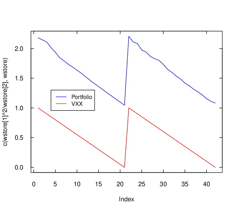
As for the strategy, we give an example in Figure 9 over two contract cycles. Interestingly, the dynamic strategy is quite linear falling from a little over 2 in value to 1 by maturity. This indicates that the strategy is also short %100 of its value in 2-month futures rising to 0% by maturity of the 1-month futures. For comparison, we also plot the strategy of VXX, which is linear from 1 to 0 over each contract cycle.




6 Concluding Remarks
In this paper we have presented the construction of static and dynamic portfolios of VIX futures that are optimized for VIX tracking. As discussed from both empirical and theoretical perspectives, futures prices tend not to react quickly enough to movements in the spot VIX. They also bring persistent negative returns and thus makes tracking VIX difficult. In view of the pitfalls of static portfolios, we design and implement a dynamic trading strategy that adjusts futures positions daily to optimally replicate VIX’s returns. The model is calibrated to historical data and a simulation study is performed to understand the properties exhibited by the strategy. In addition, comparing to the volatility ETN, VXX, we find that our dynamic strategy has a superior tracking performance.
There are a number of directions for future research. The question of how well ETFs or ETNs track their reference index is not limited to VIX-based products. It is relevant and important for all other asset classes, ranging from equities to commodities.1313 13 See Guo and Leung 2015 for a study on the tracking performance of commodity ETFs. In our static replicating portfolios, we have chosen to include futures only for comparison to VXX. Alternatively, one can also construct a static portfolio of options and optimize to minimize tracking errors with respect to an index or its leveraged exposure (see Leung and Lorig 2016). It would be interesting to compare the tracking performance of portfolios with different derivatives. Strategies and instruments aside, a major challenge in all tracking problems is to properly model the evolution of the index. Hence, accurate predictions of the index movements can potentially enhance tracking performance. To that end, one future research direction is to apply machine learning techniques to incorporate predictive analytics into the tracking problem.
References
- Black (1976) Black, F. (1976). Studies of stock price volatility changes. In Proceedings of the 1976 Meetings of the American Statistical Association, Business and Economics Statistics Section, pages 177–181.
- Cox et al. (1985) Cox, J. C., Ingersoll, J. E., and Ross, S. A. (1985). A theory of the term structure of interest rates. Econometrica, 53(2):385–408.
- Deng et al. (2012) Deng, G., McCann, C., and Wang, O. (2012). Are VIX futures ETPs effective hedges? The Journal of Index Investing, 3(3):35–48.
- Eraker and Wu (2013) Eraker, B. and Wu, Y. (2013). Explaining the negative returns to VIX futures and ETNs: An equilibrium approach. Working paper.
- Grübichler and Longstaff (1996) Grübichler, A. and Longstaff, F. (1996). Valuing futures and options on volatility. Journal of Banking and Finance, 20(6):985–1001.
- Guo and Leung (2015) Guo, K. and Leung, T. (2015). Understanding the tracking errors of commodity leveraged ETFs. In Aid, R., Ludkovski, M., and Sircar, R., editors, Commodities, Energy and Environmental Finance, Fields Institute Communications. Springer.
- Guo and Leung (2017) Guo, K. and Leung, T. (2017). Understanding the non-convergence of agricultural futures via stochastic storage costs and timing options. Journal of Commodity Markets, 6:32–49.
- Jiao (2016) Jiao, L. (2016). Trading vix futures under mean reversion with regime switching. International Journal on Financial Engineering.
- Leung et al. (2016) Leung, T., Li, J., Li, X., and Wang, Z. (2016). Speculative futures trading under mean reversion. Asia-Pacific Financial Markets, 23(4):281–304.
- Leung and Li (2016) Leung, T. and Li, X. (2016). Optimal Mean Reversion Trading: Mathematical Analysis and Practical Applications. Modern Trends in Financial Engineering. World Scientific Publishing Company.
- Leung and Lorig (2016) Leung, T. and Lorig, M. (2016). Optimal quadratic static hedging. Quantitative Finance, 9(16):1341–1355.
- Leung and Ward (2015) Leung, T. and Ward, B. (2015). The golden target: Analyzing the tracking performance of leveraged gold ETFs. Studies in Economics and Finance, 32(3):278–297.
- Leung and Ward (2018) Leung, T. and Ward, B. (2018). Dynamic index tracking and risk exposure control using derivatives. Applied Mathematical Finance, 25(2):180–212.
- Leung and Yan (2018) Leung, T. and Yan, R. (2018). Optimal dynamic pairs trading of futures under a two-factor mean-reverting model. International Journal of Financial Engineering, 5(3):1850027.
- Leung and Yan (2019) Leung, T. and Yan, R. (2019). A stochastic control approach to managed futures portfolios. International Journal of Financial Engineering, 6(1):1950005.
- Mencia and Sentana (2013) Mencia, J. and Sentana, E. (2013). Valuation of VIX derivatives. Journal of Financial Economics, 108:367–391.
- Pavlova and Daigler (2008) Pavlova, I. and Daigler, R. T. (2008). The non-convergence of VIX futures at expiration. Review of Futures Markets, 17(2):201–223.
- Uhlenbeck and Ornstein (1930) Uhlenbeck, G. E. and Ornstein, L. S. (1930). On the theory of the Brownian motion. Physical Review, 36(5):823–841.
- Ward (2017) Ward, B. (2017). Optimal Dynamic Strategies for Index Tracking and Algorithmic Trading. PhD thesis, Columbia University.
- Whaley (2013) Whaley, R. E. (2013). Trading volatility: At what cost? The Journal of Portfolio Management, 40(1):95–108.
- Zhang and Zhu (2006) Zhang, J. E. and Zhu, Y. (2006). VIX futures. Journal of Futures Markets, 26(6):521–531.