跳到论文正文
W Papers独立论文阅读器 arXiv:1907.00173 论文正文 计算阅读时间 · 0%
引用这篇论文根据当前论文元数据生成,正式投稿前建议核对。


License: CC BY-NC-ND 4.0
arXiv:1907.00173v7 [cs.IT] 02 Dec 2020

Fast Accurate Beam and Channel Tracking for Two-dimensional Phased Antenna Arrays

Yu Liu    Jiahui Li    Xiujun Zhang Affiliation: National Laboratory for Information Science and Technology, Tsinghua University, Beijing, 100084, China    Shidong Zhou
Abstract

The sparsity and the severe attenuation of millimeter-wave (mmWave) channel imply that highly directional communication is needed. The narrow beam produced by large array requires accurate alignment, which is difficult to achieve when serving fast-moving users. In this paper, we focus on accurate two-dimensional (2D) beam and channel tracking problem aiming at minimizing exploration overhead and tracking error. Using a typical frame structure with periodic exploration and communication, a proven minimum overhead of exploration is provided first. Then tracking algorithms are designed for three types of channels with different dynamic properties. It is proved that the algorithms for quasi-static channels and channels in Dynamic Case I are optimal in approaching the minimum Cramér-Rao lower bound (CRLB). The computational complexity of our algorithms is analyzed showing their efficiency, and simulation results verify their advantages in both tracking error and tracking speed.

Index Terms: 
Millimeter-wave mobile communication, beam and channel tracking, 2D phased antenna array, optimal exploring beam, Cramér-Rao lower bound.

I Introduction

Millimeter-wave (mmWave) mobile communication is currently a hot topic due to its much wider bandwidth compared with the sub-6GHz spectrum. In mmWave channels, the much higher frequency leads to severe propagation loss, atmospheric absorption, penetration loss and other obstructions [1]. Fortunately, the shorter wavelength in the mmWave band allows the deployment of a larger antenna array, providing a considerable beamforming gain to compensate for the path loss [2, 3, 4, 5, 6]. For a hybrid or analog beamforming (ABF) system as cost-efficient ways to obtain this array gain, misalignment of beam direction may not only degrade the effective receiving power, increasing mutual interference, but also lead to the loss of beam observations due to the users’ mobility, especially in fast-varying environments [7, 8]. Therefore, accurate beam tracking is crucial for serving fast-moving users in mmWave mobile communication system.

In this paper, we will focus on the problem in ABF. Since only one RF chain connected with the antennas via programmable phase shifters is available in ABF, only one set of phase shifts can be applied (forming a so-called exploring beamforming vector (EBV) in this paper) and one dimension of the multiple-antenna channel can be observed at a certain time. Hence, in order to estimate the direction and the gain of the beam, the transceiver needs to try several different EBVs one by one. These EBVs can have a significant impact on tracking performance [9, 10, 11].

Although there already exist some beam tracking methods in [12, 13, 14, 15, 7, 16], which utilized historical exploring directions and observations to obtain current estimates, the EBVs were not optimized in those tracking algorithms. While beamforming resulting in the highest combining signal-to-noise ratio (SNR) is the best for data transmission, it is not the best for tracking accuracy [10, 11]. Optimal design of EBVs is necessary to achieve as accurate beam alignment as possible in mmWave mobile communication.

In [9], a beam tracking algorithm was proposed, trying to optimize the EBVs, assuming that the channel gain is known. In [10], the authors started to jointly track the channel gain and the beam direction with optimal EBVs. In [11], the optimization of the EBVs is converted to a convex problem and solved by online optimization toolboxes. Despite the progress, only one-dimensional (1D) array is supported for beam tracking optimization in these works. However, in most mobile applications, two-dimensional (2D) arrays are necessary, not only for providing much higher array gain, but also for supporting both horizontal and vertical beam direction variation [17, 18]. It brings huge challenges when extending the optimal EBVs in [10, 11] to 2D arrays. The optimization of the exploring directions in [10] relies on the symmetrical property of the two exploring beams, however, keeping this symmetrical property may result in more overhead when extended to 2D tracking. As for the algorithm in [11], the objective function versus the EBVs becomes extremely complicated and quite different in 2D tracking compared with 1D tracking, leading to the failure of the previously used optimization method in 1D system. To the best of the authors’ knowledge, there is no work on the design of optimal EBVs for 2D array yet.
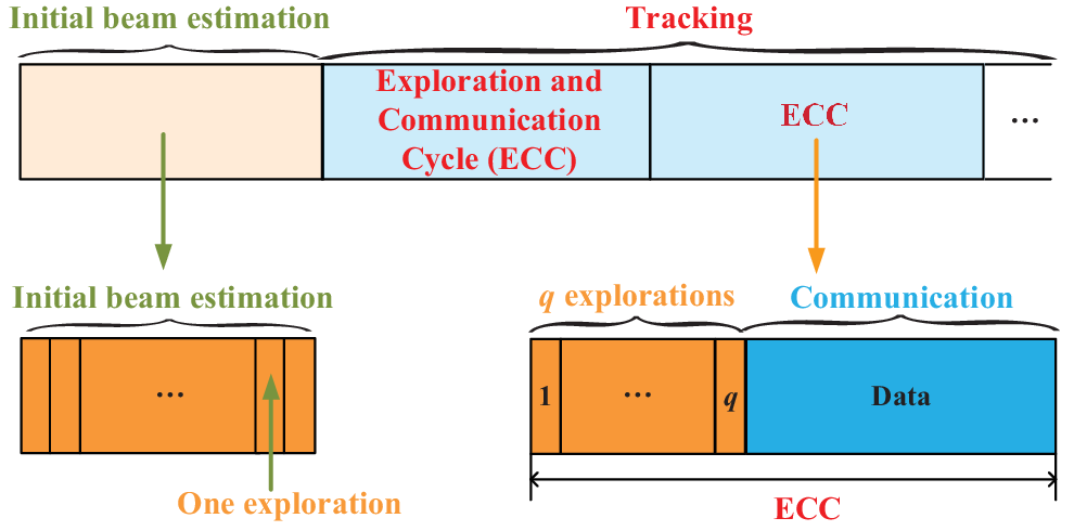
Refer to caption
Fig. 1: The frame structure for tracking.

In this paper, we focus on the design of the optimal EBVs and the accurate single-path tracking algorithms based on 2D phased antenna array. The widely used frame structure [10, 8, 19] is adopted here. As shown in Fig. 1, the transceiver periodically works in exploration and communication mode. In the exploration stage of each exploration and communication cycle (ECC), the transmitter sends a pre-defined pilot sequence for qq times. At each time, the receiver forms one exploring beam pointing in one direction to observe the channel. Then the channel gain and the direction of the incoming beam are estimated with the qq observations of the channel. In the communication stage of each ECC, the beam is aligned in the current estimated direction, and the current estimated channel gain will be used for the subsequent process. Based on this structure, the following questions are to be answered:

1) What is the minimum exploration overhead qq in each ECC for 2D tracking?

2) How to determine the qq exploring directions based on the channel observations in previous ECCs for 2D tracking?

3) How to track the 2D beam direction and the channel gain for different time-varying channels, e.g., from quasi-static channels to fast-fading channels?

4) How is the accuracy, convergence and stability of the tracking algorithm?

Following these questions, we summarize the main contributions of this paper as below:

1) Based on a reasonable EBV constraint, it is proved that the minimum exploration overhead counted by the number of exploring directions is q=3q=3, for a unique solution of the 2D beam direction and the channel gain within only one ECC, while simple extension from 1D to 2D tracking will need q=4q=4.

2) Dynamic beam and channel tracking strategies for three different time-varying channels (called Quasi-static Case, Dynamic Case I and Dynamic Case II in this paper) are proposed and optimized. The salient advantages of these tracking algorithms are given below:

i) In Quasi-static Case (channels with quasi-static beam direction and channel gain), the optimal exploration offsets are derived. Also, a joint beam direction and channel gain tracking algorithm is proposed, and the tracking error is proved to converge to the minimum Cramér-Rao lower bound (CRLB).

ii) In Dynamic Case I (channels with quasi-static beam direction and fast-fading channel gain), the Rayleigh fading channel is studied as a special case in this paper. The optimal exploration offsets are obtained and an algorithm for beam (only) tracking is proposed, which is proved to converge and achieve the minimum CRLB on the beam direction.

iii) In Dynamic Case II (channels with fast-changing beam direction and channel gain), a joint tracking algorithm of the beam direction and the channel gain is proposed with faster and more accurate performance.

3) The impact of the antenna pattern on the tracking algorithms and the performance is taken into account, showing that the proposed algorithms are suitable for practical implementations.

Part of this work was presented in our conference paper [20], while the main difference and novelty of this paper lies in the following four aspects: 1) tracking with a general antenna pattern rather than a simple isotropic pattern: we consider a more general direction-dependent antenna element pattern here rather than an isotropic pattern; 2) tracking for different types of time-varying channels: in addition to slow-fading channels, fast-fading channels are also studied in this paper and the corresponding tracking strategy is proposed and optimized, while the prior algorithm does not support fast-fading channels; 3) the complexity analysis: we analyze the computational complexity of the proposed tracking algorithms while this was missing in our previous work; 4) more rigorous conclusions and more complete proofs: we provide more rigorous lemmas and theorems with more complete proofs in this paper, correcting the corresponding flaws in the previous work.

The remaining part of this paper is organized as follows: the system model is described in Section II. In Section III, the tracking problem with some constraints is formulated. Then the minimum exploration overhead of joint 2D beam and channel tracking is given in theory in Section IV. In Section V and Section VI, the tracking problems for Quasi-static Case (Section V) and Dynamic Case I (Section VI) are studied separately. The tracking performance bounds are derived and corresponding tracking algorithms are developed with convergence and optimality analysis. In Section VII, a tracking algorithm is developed for Dynamic Case II. Then the complexity analysis of these algorithms is given in Section VIII. Section IX presents numerical results to verify the performance of our proposed algorithms.

Notations: We use lower case letters such as aa and a to denote scalars and column vectors. Respectively, |a|\lvert\textbf{a}\rvert and ‖a‖2\left\|\textbf{a}\right\|_{2} represent the modulus and 2-norm of the vector a. Upper case boldface letters, e.g., A, are used to denote matrices. The superscript (⋅)¯\bar{\left(\cdot\right)}, (⋅)T\left(\cdot\right)^{\text{T}}, (⋅)H\left(\cdot\right)^{\text{H}} are utilized to denote conjugate, transpose and conjugate-transpose. For a matrix A, its inverse, pseudo-inverse and determinant are written as A−1\textbf{A}^{-1}, A+\textbf{A}^{+} and |A|\lvert\textbf{A}\rvert. The identity matrix of order qq is denoted by Jq\textbf{J}_{q}. Let 𝒞​𝒩​(μ,σ2)\mathcal{CN}(\mu,\sigma^{2}) represent the symmetric complex Gaussian distribution with mean μ\mu and variance σ2\sigma^{2}, and 𝒩⁡(μ,σ2)\mathcal{N}(\mu,\sigma^{2}) stand for the real Gaussian distribution with mean μ\mu and variance σ2\sigma^{2}. The Kronecker product is represented as ⊗\otimes. The statistical expectation is denoted by 𝔼⁡[⋅]\mathbb{E}\left[\cdot\right]. The real (imaginary) part is represented as Re​{⋅}\text{Re}\left\{\cdot\right\} (Im​{⋅})\left(\text{Im}\left\{\cdot\right\}\right). The natural logarithm of a scalar yy is obtained by log⁡(⋅)\log\left(\cdot\right) and the phase angle of a complex number zz is written as ∠​z\angle z. The main acronyms used in this paper are summarized in TABLE I.

TABLE I: Summary of the main acronyms.
Cramér-Rao lower bound CRLB
analog beamforming ABF
exploring beamforming vector EBV
exploration and communication cycle ECC
direction parameter vector DPV
exploring beamforming matrix EBM
joint beam and channel tracking JBCT
recursive beam tracking RBT

II System Model

II-A System Configuration

We consider a mmWave receiver11 1  Note that tracking is needed at both the transmitter and the receiver. However, considering the transmitter-receiver reciprocity, the tracking of both sides have similar designs. Hence, we focus on beam and channel tracking at the receiver side. equipped with a planar phased antenna array, as shown in Fig. 2. The planar array consists of M×NM\times N antenna elements that are placed in a rectangular area, where MM(NN) antenna elements are evenly distributed along xx-axis (zz-axis) with a distance d1d_{1} (d2d_{2}) between neighboring elements. These antenna elements are connected to the same RF chain via programmable phase shifters.

Single RF chain of ABF makes a constraint that only one beam can be formed at any time and hence the receiver has to work alternatively in exploration and communication mode, resulting in a frame structure of periodic ECC. The angle of arrival (AoA) and the channel gain are assumed to be constant in each ECC and may change in different ECCs. In the exploration stage of one ECC, the transmitter sends a pre-defined pilot sequence s for qq times, where s=[s1,⋯,sLs]∈ℂ1×Ls\textbf{s}=\left[s_{1},\cdots,s_{L_{s}}\right]\in\mathbb{C}^{1\times L_{s}} contains LsL_{s} same symbols. At each time, the receiver forms one exploring beam pointing in one direction to observe the channel. Then the channel gain and the direction of the incoming beam are estimated according to the qq observations obtained in the current and previous ECCs. In the communication stage of each ECC, the beam is aligned in current estimated direction, and the current estimated channel gain will be used for the subsequent process.

II-B Channel Model

In mmWave outdoor communication, the scattering is not rich and the number of effective propagation paths is usually limited [1, 21]. Besides, the beam formed by a large array in the mmWave system is quite narrow and the interaction between multi-path is relatively weak [22]. In other words, the incoming paths are usually sparse in space, making it possible to track each path independently. Hence, we focus on the method for tracking one path, while different paths can be tracked separately by using the same method.

Refer to caption
Fig. 2: MmWave receiver with 2D phased antenna array.

In kk-th ECC, the direction of the incoming beam is denoted by (θk,ϕk\theta_{k},\phi_{k}), where θk∈[−π2,π2)\theta_{k}\in[-\frac{\pi}{2},\frac{\pi}{2}) is the elevation AoA and ϕk∈[0,π)\phi_{k}\in[0,\pi) is the azimuth AoA. Then the channel vector of this path during kk-th ECC is

hk=η⁡(θk,ϕk)​βkc​a​(xk),\textbf{h}_{k}=\eta\left(\theta_{k},\phi_{k}\right)\beta_{k}^{c}\textbf{a}(\textbf{x}_{k}), (1)

where η⁡(θ,ϕ)\eta\left(\theta,\phi\right) is the direction-dependent antenna gain (antenna pattern) of each element,22 2  Note that the antenna patterns of different elements in the array may not be exactly the same and need to be carefully calibrated. However, considering that it is not the focus of this paper, we assume the same patterns for all the elements here. βkc\beta_{k}^{c} is the complex channel gain, xk≜[xk,1,xk,2]T=[M​d1​cos⁡(θk)​cos⁡(ϕk)λ,\textbf{x}_{k}\triangleq\left[x_{k,1},x_{k,2}\right]^{\text{T}}=\big[\frac{Md_{1}\cos(\theta_{k})\cos(\phi_{k})}{\lambda}, N​d2​sin⁡(θk)λ]T\frac{Nd_{2}\sin(\theta_{k})}{\lambda}\big]^{\text{T}}is the direction parameter vector (DPV) determined by (θk,ϕk\theta_{k},\phi_{k}),

a​(xk)=a1​(xk,1)⊗a2​(xk,2)\textbf{a}(\textbf{x}_{k})=\textbf{a}_{1}\left(x_{k,1}\right)\otimes\textbf{a}_{2}\left(x_{k,2}\right) (2)

is the 2D steering vector with

a1​(xk,1)≜[1,ej​2​π​xk,1M,⋯,ej​2​π​M−1M​xk,1]T\displaystyle\textbf{a}_{1}({x}_{k,1})\triangleq\left[1,e^{j2\pi\frac{x_{k,1}}{M}},\cdots,e^{j2\pi\frac{M-1}{M}x_{k,1}}\right]^{\text{T}} (3)
a2​(xk,2)≜[1,ej​2​π​xk,2N,⋯,ej​2​π​N−1N​xk,2]T,\displaystyle\textbf{a}_{2}({x}_{k,2})\triangleq\left[1,e^{j2\pi\frac{x_{k,2}}{N}},\cdots,e^{j2\pi\frac{N-1}{N}x_{k,2}}\right]^{\text{T}}, (4)

and λ\lambda is the wavelength. For the convenience of expression, the antenna gain η⁡(θk,ϕk)\eta\left(\theta_{k},\phi_{k}\right) is denoted by η⁡(xk)\eta\left(\textbf{x}_{k}\right) hereinafter.

Define the equivalent channel gain in kk-th ECC as below:

β⁡(xk)≜η⁡(xk)​βkc,\beta\left(\textbf{x}_{k}\right)\triangleq\eta\left(\textbf{x}_{k}\right)\beta_{k}^{c}, (5)

then the channel vector in (1) can be rewritten as

hk=β⁡(xk)​a​(xk).\textbf{h}_{k}=\beta\left(\textbf{x}_{k}\right)\textbf{a}(\textbf{x}_{k}). (6)

II-C RF and Baseband Preprocessing

Synchronization in both carrier frequency and symbol timing is necessary in mmWave wireless communications. In the initial beam estimation stage in Fig. 1, the carrier frequency synchronization information can be obtained and estimated, the residual error of which can be converted to the time-varying phase of the equivalent channel gain in (5). As for the symbol timing, since it changes much slower, it can be estimated and tracked much more easily both in the initial beam estimation stage and the tracking stage. There already exists a lot of work on the synchronization algorithms in mmWave communication systems [23, 24, 25]. To make the research goals more focused, we assume perfect synchronization in this paper. Future work may be needed to further study the impact of residual synchronization error on the beam tracking performance.

Next, we will focus on the receiving beamforming based on the perfect synchronization assumption above. Let wk,i∈ℂM​N×1\textbf{w}_{k,i}\in\mathbb{C}^{MN\times 1} be the EBV for receiving the pilot sequence s the ii-th (i=1,⋯,q)(i=1,\cdots,q) time in kk-th ECC. The entries of wk,i\textbf{w}_{k,i} are of the same amplitude with |[wk,i]l|=1M​N\bigg|\left[\textbf{w}_{k,i}\right]_{l}\bigg|=\frac{1}{\sqrt{MN}}, where [wk,i]l\left[\textbf{w}_{k,i}\right]_{l} denotes the ll-th element of wk,i\textbf{w}_{k,i}. After phase shifting and combining, the ii-th received sequence in kk-th ECC at the baseband output of the RF chain is given by

𝝂k,i=β⁡(xk)​wk,iH​a​(xk)​s+𝜻k,i.\boldsymbol{\nu}_{k,i}=\beta\left(\textbf{x}_{k}\right)\textbf{w}_{k,i}^{\text{H}}\textbf{a}(\textbf{x}_{k})\textbf{s}+\boldsymbol{\zeta}_{k,i}. (7)

where 𝜻k,i∈ℂ1×Ls\boldsymbol{\zeta}_{k,i}\in\mathbb{C}^{1\times L_{s}} is the receiving noise vector.

By match filtering on the sequence 𝝂k,i\boldsymbol{\nu}_{k,i}, the ii-th observation in kk-th ECC is given below:

yk,i=𝝂k,i​sH|s|=\displaystyle{y}_{k,i}=\boldsymbol{\nu}_{k,i}\frac{\textbf{s}^{\text{H}}}{\lvert\textbf{s}\rvert}= β⁡(xk)​wk,iH​a​(xk)​s​sH|s|+𝜻k,i​sH|s|\displaystyle\beta\left(\textbf{x}_{k}\right)\textbf{w}_{k,i}^{\text{H}}\textbf{a}(\textbf{x}_{k})\textbf{s}\frac{\textbf{s}^{\text{H}}}{\lvert\textbf{s}\rvert}+\boldsymbol{\zeta}_{k,i}\frac{\textbf{s}^{\text{H}}}{\lvert\textbf{s}\rvert} (8)
=\displaystyle= |s|​β​(xk)​wk,iH​a​(xk)+zk,i,\displaystyle\lvert\textbf{s}\rvert\beta\left(\textbf{x}_{k}\right)\textbf{w}_{k,i}^{\text{H}}\textbf{a}(\textbf{x}_{k})+{z}_{k,i},

where zk,i≜𝜻k,i​sH|s|z_{k,i}\triangleq\boldsymbol{\zeta}_{k,i}\frac{\textbf{s}^{\text{H}}}{\lvert\textbf{s}\rvert} is an additive noise, which is modeled as i.i.d. Gaussian distributed in this paper, i.e., zk,i∼𝒞​𝒩​(0,σz2)z_{k,i}\sim\mathcal{CN}\left(0,\sigma_{z}^{2}\right). This assumption is certainly held when the receiving noise vector 𝜻k,i\boldsymbol{\zeta}_{k,i} is i.i.d. Gaussian distributed. Besides, even when the noise vector 𝜻k,i\boldsymbol{\zeta}_{k,i} is non-Gaussian, if the real and imaginary parts of the elements in 𝜻k,i\boldsymbol{\zeta}_{k,i} are i.i.d, the observation noise zk,iz_{k,i} can also be regarded as i.i.d. Gaussian distributed as long as the pilot sequence length LsL_{s} is sufficiently large, according to the central limit theorem [26].

Let Wk≜[wk,1,…,wk,q]\textbf{W}_{k}\triangleq\left[\textbf{w}_{k,1},\ldots,\textbf{w}_{k,q}\right], zk≜[zk,1,…,zk,q]T\textbf{z}_{k}\triangleq\left[z_{k,1},\ldots,z_{k,q}\right]^{\text{T}} and yk≜[yk,1,…,yk,q]T\textbf{y}_{k}\triangleq\left[y_{k,1},\ldots,y_{k,q}\right]^{\text{T}} denote the exploring beamforming matrix (EBM), the noise vector and the observation vector respectively. Then we can rewrite (8) as follows:

yk=|s|​β​(xk)​WkH​a​(xk)+zk.\textbf{y}_{k}=\lvert\textbf{s}\rvert\beta\left(\textbf{x}_{k}\right)\textbf{W}_{k}^{\text{H}}\textbf{a}(\textbf{x}_{k})+\textbf{z}_{k}. (9)

II-D Tracking Loop

As shown in Fig. 1, an initial estimate β^0=β^0re+j​β^0im\hat{\beta}_{0}=\hat{\beta}_{0}^{\text{re}}+j\hat{\beta}_{0}^{\text{im}} and x^0=[x^0,1,x^0,2]T\hat{\textbf{x}}_{0}=\left[\hat{x}_{0,1},\hat{x}_{0,2}\right]^{\text{T}} can be obtained in the beam estimation stage. It is assumed in this paper that the initial beam estimator can output an estimate x^0\hat{\textbf{x}}_{0} falling within the main lobe of x0\textbf{x}_{0}, i.e., x^0∈ℬ⁡(x0)\hat{\textbf{x}}_{0}\in\mathcal{B}\left(\textbf{x}_{0}\right), where ℬ⁡(xt)\mathcal{B}\left(\textbf{x}_{t}\right) denotes the main lobe of an arbitrary DPV xt=[xt,1,xt,2]T\textbf{x}_{t}=\big[x_{t,1},x_{t,2}\big]^{\text{T}}, given by

ℬ⁡(xt)≜(xt,1−1,xt,1+1)×(xt,2−1,xt,2+1).\displaystyle\mathcal{B}\!\left(\textbf{x}_{t}\right)\!\triangleq\!\left(x_{t,1}-1,x_{t,1}+1\right)\!\times\!\left(x_{t,2}-1,x_{t,2}+1\right)\,. (10)

Then our tracking starts from this initial estimate x^0\hat{\textbf{x}}_{0} to find more accurate beam directions. It is worth pointing out that the main lobe in x domain in (10) has been normalized to a square with twice the unit length of each side and centered at the DPV xt\textbf{x}_{t} after the transformation from the angle domain to x domain. Hence, the main lobe size in x domain remains unchanged even if the antenna size M,NM,\,N scale.

In the exploration stage of kk-th ECC, the receiver needs to choose an EBM Wk\textbf{W}_{k} based on historical observation vectors y1,⋯,yk−1\textbf{y}_{1},\cdots,\textbf{y}_{k-1} along with the corresponding EBMs W1,⋯,Wk−1\textbf{W}_{1},\cdots,\textbf{W}_{k-1}. The new observation yk\textbf{y}_{k} can be obtained by applying Wk\textbf{W}_{k}. Then the estimate 𝝍^k≜[β^kre,β^kim,x^k,1,x^k,2]T\hat{\boldsymbol{\psi}}_{k}\triangleq\left[\hat{\beta}_{k}^{\text{re}},\hat{\beta}_{k}^{\text{im}},\hat{x}_{k,1},\hat{x}_{k,2}\right]^{\text{T}} of the channel parameter vector 𝝍k≜[Re​{β⁡(xk)},Im​{β⁡(xk)}CLOSE,\boldsymbol{\psi}_{k}\triangleq\big[\text{Re}\left\{\beta\left(\textbf{x}_{k}\right)\right\},\text{Im}\left\{\beta\left(\textbf{x}_{k}\right)\right\}, xk,1,xk,2]Tx_{k,1},{x}_{k,2}\big]^{\text{T}} is obtained by using all observation vectors available and the corresponding EBMs. The whole tracking loop is given in Procedure 1 and the focus of this paper lies in Step 3 and Step 6.

Procedure 1 Tracking Loop
1: Array size M,NM,N and the pilot sequence s.
2: The estimate of the channel parameter vector 𝝍^k\hat{\boldsymbol{\psi}}_{k}.
3: Initialize 𝝍^0=[β^0re,β^0im,x^0,1,x^0,2]T\hat{\boldsymbol{\psi}}_{0}=\left[\hat{\beta}_{0}^{\text{re}},\hat{\beta}_{0}^{\text{im}},\hat{x}_{0,1},\hat{x}_{0,2}\right]^{\text{T}};
4: for k=1,2,⋯k=1,2,\cdots do
5:   Calculate Wk\textbf{W}_{k} based on 𝝍^0\hat{\boldsymbol{\psi}}_{0}, W1,⋯,Wk−1\textbf{W}_{1},\cdots,\textbf{W}_{k-1}, y1,⋯,yk−1\textbf{y}_{1},\cdots,\textbf{y}_{k-1};
6:   Apply Wk\textbf{W}_{k} in the exploring stage of kk-th ECC;
7:   Obtain the observation vector yk\textbf{y}_{k} in kk-th ECC;
8:   Estimate 𝝍^k\hat{\boldsymbol{\psi}}_{k} based on 𝝍^0\hat{\boldsymbol{\psi}}_{0}, W1,⋯,Wk\textbf{W}_{1},\cdots,\textbf{W}_{k}, y1,⋯,yk\textbf{y}_{1},\cdots,\textbf{y}_{k};
9:   Point to x^k\hat{\textbf{x}}_{k} in the communication stage of kk-th ECC;
10:   use β^k\hat{\beta}_{k} for receiving in the communication stage of kk-th ECC.
11: end for

From a control system perspective, 𝝍k{\boldsymbol{\psi}}_{k} is the system state, 𝝍^k\hat{{\boldsymbol{\psi}}}_{k} is the estimate of the system state, the EBM Wk\textbf{W}_{k} is the control action and yk\textbf{y}_{k} is a noisy observation non-linearly determined by the system state and the control action. Hence, the task of a tracking design is to find the following strategy:

Wk=\displaystyle\textbf{W}_{k}= Fkc​(𝝍^0,W1,⋯,Wk−1,y1,⋯,yk−1)\displaystyle\textbf{F}_{k}^{c}\left(\hat{\boldsymbol{\psi}}_{0},\textbf{W}_{1},\cdots,\textbf{W}_{k-1},\textbf{y}_{1},\cdots,\textbf{y}_{k-1}\right) (11)
𝝍^k=\displaystyle\hat{\boldsymbol{\psi}}_{k}= Fke​(𝝍^0,W1,⋯,Wk,y1,⋯,yk),\displaystyle\textbf{F}_{k}^{e}\left(\hat{\boldsymbol{\psi}}_{0},\textbf{W}_{1},\cdots,\textbf{W}_{k},\textbf{y}_{1},\cdots,\textbf{y}_{k}\right), (12)

where Fkc\textbf{F}_{k}^{c} denotes the control function and Fke\textbf{F}_{k}^{e} denotes the estimation function in kk-th ECC.

III Problem Formulation

Let Ξk={Fkc,Fke}\Xi_{k}=\left\{\textbf{F}_{k}^{c},\textbf{F}_{k}^{e}\right\} denote the set of beam and channel tracking schemes in kk-th ECC. Then the optimal beam and channel tracking problem minimizing the mean square error (MSE) of the channel vector estimate is formulated as:

minΞk\displaystyle\underset{\Xi_{k}}{\min}~ 1M​N​𝔼​[‖h^k−hk‖22]\displaystyle\frac{1}{MN}\,\mathbb{E}\left[{\left\|\hat{\textbf{h}}_{k}-\textbf{h}_{k}\right\|}_{2}^{2}\right] (13)
s.t.  𝔼⁡[h^k]=hk,\displaystyle\mathbb{E}\left[\hat{\textbf{h}}_{k}\right]=\textbf{h}_{k}, (14)
(9),(11),(12),\displaystyle\eqref{eq_observation_vector},\eqref{eq_Fc},\eqref{eq_Fe},\vskip-14.22636pt

where the constraint (14) ensures that h^k≜β^k​a​(x^k)\hat{\textbf{h}}_{k}\triangleq\hat{\beta}_{k}\textbf{a}\left(\hat{\textbf{x}}_{k}\right) is an unbiased estimate of the channel vector hk=β⁡(xk)​a​(xk)\textbf{h}_{k}=\beta\left(\textbf{x}_{k}\right)\textbf{a}\left(\textbf{x}_{k}\right). It is worth explaining the following two points. First, an unbiased estimator may not be the best estimator that achieves the minimum MSE. Nevertheless, such an optimal estimator with no constraints is hard to obtain and hence we add this unbiasedness constraint. Second, we only need to guarantee the unbiasedness of h^k\hat{\textbf{h}}_{k}, as the objective function in (13) is the MSE of the channel vector. The estimate of the equivalent channel gain and the DPV, i.e., β^k\hat{\beta}_{k} and x^k\hat{\textbf{x}}_{k}, can be biased.

Problem (13) is challenging to be solved optimally due to the following reasons:

1) It is a partially observed Markov decision process (POMDP) which generally has not been solved optimally [27, 28].

2) There are M×NM\times N phase shifts to adjust in each EBV wk,i\textbf{w}_{k,i}. This makes the optimization of the EBV too complicated due to the joint design of so many phase shifts, especially when the array size M×NM\times N grows large.

3) To obtain 𝝍^k\hat{\boldsymbol{\psi}}_{k} in kk-th ECC, kk EBMs, i.e., W1,⋯,Wk\textbf{W}_{1},\cdots,\textbf{W}_{k}, need to be designed, making it difficult to optimize so many beamforming matrices simultaneously as kk increases.

4) The time-varying features of the channel vector in (6) restrict the tracking algorithm and the system performance. Thus, it is hard to design an optimal tracking method for a general channel model.

These challenges above make it extremely difficult to solve this problem optimally. Hence, we add some reasonable constraints in this paper to take the first step of the optimal tracking policy:

III-A The EBV constraint

As it is complicated to obtain the optimal M×NM\times N phase shifts in general for each EBV, we use steering vectors to design the EBVs,

wk,i=1M​N​a​(𝝎k,i),\textbf{w}_{k,i}=\frac{1}{\sqrt{MN}}\textbf{a}\left(\boldsymbol{\omega}_{k,i}\right), (15)

where 𝝎k,i≜[ωk,i​1,ωk,i​2]T\boldsymbol{\omega}_{k,i}\triangleq\left[{\omega}_{k,i1},{\omega}_{k,i2}\right]^{\text{T}} denotes the ii-th exploring direction vector in kk-th ECC. This ensures that only two variables need to be designed for each EBV.

III-B The exploring direction constraint

Although the exploring direction vector 𝝎k,i\boldsymbol{\omega}_{k,i} in (15) can be of any form, however, considering the tracking accuracy, it is better to make sure that 𝝎k,i\boldsymbol{\omega}_{k,i} falls within the main lobe of the DPV xk\textbf{x}_{k} in (10). Thus, it is reasonable to choose exploring directions near the recently estimated direction x^k−1\hat{\textbf{x}}_{k-1}. For this purpose, we use such an architecture in this paper. That is, the ii-th exploring direction vector in kk-th ECC, i.e., 𝝎k,i\boldsymbol{\omega}_{k,i}, is determined by the previous estimate of the DPV plus an exploration offset 𝚫k,i\boldsymbol{\Delta}_{k,i}. Considering the design of the offsets that change in different ECCs is also very complicated, we adopt fixed exploration offsets 𝚫i​(i=1,⋯,q)\boldsymbol{\Delta}_{i}(i=1,\cdots,q) in this paper:

𝝎k,i=x^k−1+𝚫i,i=1,⋯,q.\boldsymbol{\omega}_{k,i}=\hat{\textbf{x}}_{k-1}+\boldsymbol{\Delta}_{i},\,i=1,\cdots,q.\vskip 0.0pt (16)

Therefore, the EBV in (15) can be rewritten as

wk,i=1M​Na(x^k−1+𝚫i),i=1,⋯,q.\textbf{w}_{k,i}=\frac{1}{\sqrt{MN}}\textbf{a}\left(\hat{\textbf{x}}_{k-1}+\boldsymbol{\Delta}_{i}\right),\,i=1,\cdots,q. (17)

III-C The time-varying channel constraint

The time-varying channel vector in (1) is determined by three parts: the antenna gain η⁡(xk)\eta\left(\textbf{x}_{k}\right), the channel gain βkc\beta_{k}^{c} and the DPV xk\textbf{x}_{k}. Since the change of the antenna gain η⁡(xk)\eta\left(\textbf{x}_{k}\right) depends on the DPV xk\textbf{x}_{k} for a given antenna element pattern, we only consider the change of the DPV xk\textbf{x}_{k} and the channel gain βkc\beta_{k}^{c} when exploring the properties of the time-varying channels. As the user motion characteristics can be quite different in various situations [29, 30, 31], both of the DPV xk\textbf{x}_{k} and the channel gain βkc\beta_{k}^{c} may change slowly or fast. Therefore, four possible cases exist, which correspond to four different practical scenarios and can be modeled as follows:

  • •

    Quasi-static Case: xk≈x,βkc≈βc\textbf{x}_{k}\approx\textbf{x},\beta_{k}^{c}\approx\beta^{c}

    When both xk\textbf{x}_{k} and βkc\beta_{k}^{c} change slowly, e.g., the user keeps static or quasi-static in a room, the antenna gain η⁡(xk)\eta\left(\textbf{x}_{k}\right) and the equivalent channel gain β⁡(xk)\beta\left(\textbf{x}_{k}\right) defined in (5) also change slowly. The channel in this case can be seen as approximately fixed. For the sake of convenience, we assume that β⁡(xk)=β=βre+j​βim\beta\left(\textbf{x}_{k}\right)=\beta=\beta^{\text{re}}+j\beta^{\text{im}}, xk=x=[x1,x2]T\textbf{x}_{k}=\textbf{x}=\left[x_{1},x_{2}\right]^{\text{T}} in this case.

  • •

    Dynamic Case: xk≈x,βk+1c≠βkc\textbf{x}_{k}\approx\textbf{x},\beta_{k+1}^{c}\neq\beta_{k}^{c}

    For channels that xk\textbf{x}_{k} changes slowly while βkc\beta_{k}^{c} changes fast, e.g., a person walks at a fast pace in a room, the beam direction can be seen as approximately fixed, i.e., xk=x\textbf{x}_{k}=\textbf{x}[29, 30]. To distinguish from other dynamic scenarios, this case is called Dynamic Case I.

  • •

    Dynamic Case: xk+1≠xk,βkc≈βc\textbf{x}_{k+1}\neq\textbf{x}_{k},\beta_{k}^{c}\approx\beta^{c}

    This case requires that the beam direction changes fast while the channel gain keeps static or quasi-static. However, in real mmWave channels, the fast change of the beam direction usually leads to the fast change of the channel gain since the propagation paths change. This case exists only when the user rotates around the base station (BS) exactly in a circle in line of sight (LOS) channels. This is not the usual case and not studied in this paper.

  • •

    Dynamic Case: xk+1≠xk,βk+1c≠βkc\textbf{x}_{k+1}\neq\textbf{x}_{k},\beta_{k+1}^{c}\neq\beta_{k}^{c}

    Both the beam direction and the channel gain in this case change fast, which happens in most fast-moving scenarios except Dynamic Case I, e.g., an unmanned aerial vehicle (UAV) flies in the sky [31]. To distinguish from Dynamic Case I, we call it Dynamic Case II.

It would be helpful to explain the following two aspects. First of all, extra algorithms need to be introduced to efficiently classify the channels according to the time-varying features. However, to make the research goals more focused in this paper, we leave the details of this classification in future work. Second, this paper only exploits the independent variation properties of βkc\beta_{k}^{c} and xk\textbf{x}_{k} in these four cases to obtain theoretical results. While in real mmWave channels, the variation of the channel gain βkc\beta_{k}^{c} and the DPV xk\textbf{x}_{k} might be interrelated [32], which are supposed to be jointly taken into account in future work.

With the above-mentioned EBV constraint, the exploring direction constraint and the time-varying channel constraint, the beam and channel tracking problem in (13) can be reformulated as:

minΞ\displaystyle\underset{\Xi}{\min}~ 1M​N​𝔼​[‖h^k−hk‖22]\displaystyle\frac{1}{MN}\,\mathbb{E}\left[{\left\|\hat{\textbf{h}}_{k}-\textbf{h}_{k}\right\|}_{2}^{2}\right] (18)
s.t.  (9),(11),(12),(14),(17).\displaystyle\eqref{eq_observation_vector},\eqref{eq_Fc},\eqref{eq_Fe},\eqref{eq_constrant1},\eqref{eq_sv}.

IV How Many Explorations Are Needed In each ECC?

Before delving into the detailed tracking process in (18), we will first study the number of explorations needed in this section.

To estimate 𝝍k{\boldsymbol{\psi}}_{k}, sufficient measurements from different exploring directions are required. For Quasi-static Case where 𝝍k{\boldsymbol{\psi}}_{k} remains unchanged, i.e., 𝝍k=𝝍≜[βre,βim,x1,x2]T{\boldsymbol{\psi}}_{k}=\boldsymbol{\psi}\triangleq\left[\beta^{\text{re}},\beta^{\text{im}},x_{1},x_{2}\right]^{\text{T}}, one exploration in each ECC is enough since sufficient measurements are available after quite a number of ECCs. Nevertheless, in dynamic case, only using one exploration in each ECC does not work well as 𝝍k{\boldsymbol{\psi}}_{k} may change fast. Hence, it is necessary to ensure that the estimate can be obtained even by using the explorations in a single ECC. Then the question becomes: under the condition above, how many explorations are needed in each ECC?

With the constraint in (15), two explorations in each ECC are sufficient to jointly track the equivalent channel gain and the 1D beam direction according to [10]. When tracking the 2D direction, it is straight forward that four explorations are feasible by separately using two explorations to track each dimension of the 2D direction. However, using four explorations will lower the system efficiency since it will cost time resources for each exploration. Hence, we may ask that can we reduce the times of exploration, or what is the minimum number of explorations required?

Then the following lemma is proposed to help determine the minimum exploration overhead qq in each ECC:

Lemma 1.

If the EBVs are of the steering vector forms, i.e., wk,i=1M​N​a​(𝝎k,i)\textbf{w}_{k,i}=\frac{1}{\sqrt{MN}}\textbf{a}\!\left(\boldsymbol{\omega}_{k,i}\right), and the observation vector in (9) is noiseless, then

1) to obtain the unique solution of the channel parameter vector 𝛙k\boldsymbol{\psi}_{k} within one ECC, the minimum exploration overhead is q=3q=3 in each ECC;

2) to obtain the unique solution of the DPV xk\textbf{x}_{k} within one ECC, the minimum exploration overhead is q=3q=3 in each ECC.

Proof.

See Appendix A. ∎

Lemma 1 reveals that it is impossible to obtain the unique solution within one ECC when only using two explorations, whether we want to jointly estimate β⁡(xk)\beta\left(\textbf{x}_{k}\right) and xk\textbf{x}_{k} or just estimate xk\textbf{x}_{k}. If we use three explorations and design three appropriate exploring directions in each ECC, then the unique solution of the channel parameter vector 𝝍k\boldsymbol{\psi}_{k} can be obtained. Hence, we set q=3q=3 in this paper, i.e., the EBM Wk=[wk,1,wk,2,wk,3]\textbf{W}_{k}=\left[\textbf{w}_{k,1},\textbf{w}_{k,2},\textbf{w}_{k,3}\right].

V Quasi-static Tracking: Performance Bound, Convergence and Optimality

In this section, we will focus on Quasi-static Case. As mentioned in Section III, in Quasi-static Case, 𝝍k=𝝍=[βre,βim,x1,x2]T\boldsymbol{\psi}_{k}=\boldsymbol{\psi}=\left[\beta^{\text{re}},\beta^{\text{im}},x_{1},x_{2}\right]^{\text{T}} and hk=h≜β​a​(x)\textbf{h}_{k}=\textbf{h}\triangleq{\beta}\textbf{a}\left({\textbf{x}}\right). For a given channel parameter vector 𝝍\boldsymbol{\psi} and EBM Wk\textbf{W}_{k}, the observation vector satisfies normal distribution with yk∼𝒞​𝒩​(|s|​β​WkH​a​(x),σz2​J3)\textbf{y}_{k}\sim\mathcal{CN}\left(\lvert\textbf{s}\rvert\beta\textbf{W}_{k}^{\text{H}}\textbf{a}(\textbf{x}),\sigma_{z}^{2}\textbf{J}_{3}\right). Hence, the conditional probability density function of yk\textbf{y}_{k} is given by

pS​(yk|𝝍,Wk)=1π3​σz6​e−‖yk−|s|​β​WkH​a​(x)‖22σz2.p_{S}(\textbf{y}_{k}|\boldsymbol{\psi},\textbf{W}_{k})={\frac{1}{\pi^{3}\sigma_{z}^{6}}e^{-\frac{{\left\|\textbf{y}_{k}-\lvert\textbf{s}\rvert\beta\textbf{W}_{k}^{\text{H}}\textbf{a}(\textbf{x})\right\|}_{2}^{2}}{\sigma_{z}^{2}}}}. (19)

In this section, we will first provide the lower bound of the tracking error in Quasi-static Case. Then we develop a tracking algorithm and prove it can converge to the minimum CRLB with time.

V-A Cramér-Rao Lower Bound of The Tracking Error

The Cramér-Rao lower bound theory gives the lower bound of the unbiased estimation error [33]. Based on this, we introduce the following lemma to obtain the lower bound of the tracking error in Quasi-static Case:

Lemma 2.

In Quasi-static Case, given W1,⋯,Wk\textbf{W}_{1},\cdots,\textbf{W}_{k}, the MSE of the channel vector estimate in (18) is lower bounded as follows:

1M​N​𝔼​[‖h^k−h‖22]\displaystyle\,\frac{1}{{MN}}\mathbb{E}\left[\left\|\hat{\textbf{h}}_{k}-\textbf{h}\right\|_{2}^{2}\right] (20)
≥\displaystyle\geq 1M​N​Tr⁡{(∑l=1kIS​(𝝍,𝐖l))−1​(VH​V)}\displaystyle\,\frac{1}{{MN}}\Tr\left\{{{{\left(\sum\limits_{l=1}^{k}{\textbf{I}_{S}(\boldsymbol{\psi},{{\bf{W}}_{l}})}\right)}^{-1}}{\left({\textbf{V}^{\text{H}}}{\textbf{V}}\right)}}\right\}
≜\displaystyle\triangleq CSt​(𝝍,W1,⋯,Wk),\displaystyle\,{C}_{S}^{t}\left(\boldsymbol{\psi},\textbf{W}_{1},\cdots,\textbf{W}_{k}\right),

where V is the Jacobian matrix given by

V≜∂h∂𝝍T=\displaystyle\textbf{V}\triangleq\frac{{\partial\textbf{h}}}{{\partial{{\boldsymbol{\psi}}^{\text{T}}}}}= [∂h∂βre,∂h∂βim,∂h∂x1,∂h∂x2]\displaystyle\left[\frac{\partial{\textbf{h}}}{\partial{\beta^{\text{re}}}},\frac{\partial{\textbf{h}}}{\partial{\beta^{\text{im}}}},\frac{\partial{\textbf{h}}}{\partial{x_{1}}},\frac{\partial{\textbf{h}}}{\partial{x_{2}}}\right] (21)
=\displaystyle= [a​(x),j​a​(x),β​∂a​(x)∂x1,β​∂a​(x)∂x2]\displaystyle\left[\textbf{a}\left(\textbf{x}\right),j\textbf{a}\left(\textbf{x}\right),\beta\frac{\partial\textbf{a}\left(\textbf{x}\right)}{\partial x_{1}},\beta\frac{\partial\textbf{a}\left(\textbf{x}\right)}{\partial x_{2}}\right]

and the Fisher information matrix IS​(𝝍,Wl)\textbf{I}_{S}(\boldsymbol{\psi},\textbf{W}_{l}) is given by

IS​(𝝍,Wl)\displaystyle\!\textbf{I}_{S}(\boldsymbol{\psi},\textbf{W}_{l}) ≜𝔼⁡[∂log​pS​(yl|𝝍,Wl)∂𝝍⋅∂log​pS​(yl|𝝍,Wl)∂𝝍T]\displaystyle\triangleq\mathbb{E}\left[\frac{\partial\text{log}\,p_{S}\left(\textbf{y}_{l}|\boldsymbol{\psi},\textbf{W}_{l}\right)}{\partial\boldsymbol{\psi}}\!\cdot\!\frac{\partial\text{log}\,p_{S}\left(\textbf{y}_{l}|\boldsymbol{\psi},\textbf{W}_{l}\right)}{\partial\boldsymbol{\psi}^{\text{T}}}\right]
=2​|s|2σz2​Re​{VH​Wl​WlH​V}.\displaystyle=\frac{2{\lvert\textbf{s}\rvert}^{2}}{{\sigma}_{z}^{2}}\text{Re}\left\{\textbf{V}^{\text{H}}\textbf{W}_{l}\textbf{W}_{l}^{\text{H}}\textbf{V}\right\}. (22)
Proof.

See Appendix B. ∎

The CRLB in (20) is a function of the EBMs W1,…,Wk\textbf{W}_{1},\ldots,\textbf{W}_{k}. Since it is hard to optimize so many EBMs simultaneously, we will first try to find a lower bound of the CRLB under the constraint (17), and later design a tracking algorithm approaching this lower bound.

Consider any tracking algorithm under the constraint (17) that can converge to the DPV x, i.e.,

limk→+∞x^k=x.{\lim\limits_{k\to+\infty}}\hat{\textbf{x}}_{k}=\textbf{x}.\vskip 0.0pt (23)

Then the EBM Wk\textbf{W}_{k} also converges,

limk→+∞Wk=W=[w1,w2,w3]T,{\lim\limits_{k\to+\infty}}{\textbf{W}}_{k}=\textbf{W}=\left[\textbf{w}_{1},\textbf{w}_{2},\textbf{w}_{3}\right]^{\text{T}},\vskip 0.0pt (24)

where wi\textbf{w}_{i} is given by

wi≜1M​Na(x+𝚫S,i),i=1,2,3\textbf{w}_{i}\triangleq\frac{1}{\sqrt{MN}}\textbf{a}\left(\textbf{x}+\boldsymbol{\Delta}_{S,i}\right),i=1,2,3\vskip 0.0pt (25)

with {𝚫S,1,𝚫S,2,𝚫S,3}\left\{\boldsymbol{\Delta}_{S,1},\boldsymbol{\Delta}_{S,2},\boldsymbol{\Delta}_{S,3}\right\} denoting the fixed set of exploration offsets in Quasi-static Case. Hence, the normalized CRLB (by multiplying kk) converges as k→+∞k\to+\infty:

limk→+∞k​CSt​(𝝍,W1,⋯,Wk)\displaystyle{\lim\limits_{k\to+\infty}}k{C}_{S}^{t}(\boldsymbol{\psi},\textbf{W}_{1},\cdots,\textbf{W}_{k})
=\displaystyle= limk→+∞kM​N​Tr⁡{(∑l=1kIS​(𝝍,𝐖l))−1​(VH​V)}\displaystyle{\lim\limits_{k\to+\infty}}\frac{k}{{MN}}\Tr\left\{{{{\left(\sum\limits_{l=1}^{k}{\textbf{I}_{S}(\boldsymbol{\psi},{{\bf{W}}_{l}})}\right)}^{-1}}{\!\left({\textbf{V}^{\text{H}}}{\textbf{V}}\right)}}\right\} (26)
=\displaystyle= 1M​N​Tr⁡{IS​(𝝍,𝐖)−1​(VH​V)},\displaystyle\frac{1}{{MN}}\Tr\left\{{{{{\textbf{I}_{S}(\boldsymbol{\psi},{{\bf{W}}})}}^{-1}}{\left({\textbf{V}^{\text{H}}}{\textbf{V}}\right)}}\right\},

which is a function of 𝝍,W\boldsymbol{\psi},\,\textbf{W} and will be denoted as CS​(𝝍,W){C}_{S}(\boldsymbol{\psi},\textbf{W}).

According to (V-A), for a given channel (direction and gain), there exists an optimal EBM, which leads to the minimum normalized CRLB as a function of the channel parameter vector 𝝍\boldsymbol{\psi}:

CSmin​(𝝍)=\displaystyle{C}_{S}^{\min}(\boldsymbol{\psi})= minW⁡CS​(𝝍,W)=CS​(𝝍,WS∗).\displaystyle\min_{\textbf{W}}{C}_{S}(\boldsymbol{\psi},\textbf{W})={C}_{S}(\boldsymbol{\psi},\textbf{W}_{S}^{*}). (27)

Solving problem (27) yields WS∗=[wS,1∗,wS,2∗,wS,3∗]\textbf{W}_{S}^{*}=\left[\textbf{w}_{S,1}^{*},\textbf{w}_{S,2}^{*},\textbf{w}_{S,3}^{*}\right] with

wS,i∗=1M​Na(x+𝚫S,i∗),i=1,2,3,\textbf{w}_{S,i}^{*}=\frac{1}{\sqrt{MN}}\textbf{a}\left(\textbf{x}+\boldsymbol{\Delta}_{S,i}^{*}\right),i=1,2,3,\vskip 0.0pt (28)

where {𝚫S,1∗,𝚫S,2∗,𝚫S,3∗}\left\{\boldsymbol{\Delta}_{S,1}^{*},\boldsymbol{\Delta}_{S,2}^{*},\boldsymbol{\Delta}_{S,3}^{*}\right\} denotes the optimal set of exploration offsets for a given array size and a given 𝝍\boldsymbol{\psi}.

V-B Asymptotically Optimal Set of Exploration Offsets

In general, the minimum CRLB in (27) is a function of a set of system parameters including the equivalent channel gain β\beta, the DPV x and the array size M,NM,\,N. Hence, the optimal set of 2D exploration offsets should also be a function of these parameters. Since it is very hard to obtain the expression of this optimal set, we adopt numerical search to deal with this issue. However, as many parameters in (27) may affect the optimal result, numerical search has to be reconducted for different parameter sets, resulting in high complexity.

Fortunately, through our investigation, some useful properties of the minimum CRLB and the optimal set of exploration offsets are given to simplify the numerical search, as described in the following lemma:

Lemma 3.

In Quasi-static Case, the minimum CRLB CSmin​(𝛙){C}_{S}^{\min}(\boldsymbol{\psi}) and the optimal set of exploration offsets {𝚫S,1∗,𝚫S,2∗,𝚫S,3∗}\left\{\boldsymbol{\Delta}_{S,1}^{*},\boldsymbol{\Delta}_{S,2}^{*},\boldsymbol{\Delta}_{S,3}^{*}\right\} have the following three properties:

1) CSmin​(𝝍){C}_{S}^{\min}(\boldsymbol{\psi}), {𝚫S,1∗,𝚫S,2∗,𝚫S,3∗}\left\{\boldsymbol{\Delta}_{S,1}^{*},\boldsymbol{\Delta}_{S,2}^{*},\boldsymbol{\Delta}_{S,3}^{*}\right\} are invariant to the equivalent channel gain β\beta;

2) CSmin​(𝝍){C}_{S}^{\min}(\boldsymbol{\psi}), {𝚫S,1∗,𝚫S,2∗,𝚫S,3∗}\left\{\boldsymbol{\Delta}_{S,1}^{*},\boldsymbol{\Delta}_{S,2}^{*},\boldsymbol{\Delta}_{S,3}^{*}\right\} are invariant to the DPV x;

3) CSmin​(𝝍){C}_{S}^{\min}(\boldsymbol{\psi}) converges as ​M,​N→+∞\emph{M},\,\emph{N}\to+\infty and there exists a fixed set of exploration offsets that are unrelated to the array size M,NM,N, denoted as {𝚫~S,1∗,𝚫~S,2∗,𝚫~S,3∗}\left\{\widetilde{\boldsymbol{\Delta}}_{S,1}^{*},\,\widetilde{\boldsymbol{\Delta}}_{S,2}^{*},\widetilde{\boldsymbol{\Delta}}_{S,3}^{*}\right\}, such that

limM,N→+∞CS​(𝝍,W~S∗)=limM,N→+∞CSmin​(𝝍),\displaystyle{\lim\limits_{M,N\to+\infty}}{C}_{S}(\boldsymbol{\psi},\widetilde{\textbf{W}}_{S}^{*})={\lim\limits_{M,N\to+\infty}}{C}_{S}^{\min}(\boldsymbol{\psi}),\vskip 0.0pt

where W~S∗=[w~S,1∗,w~S,2∗,w~S,3∗]\widetilde{\textbf{W}}_{S}^{*}=[\tilde{\textbf{w}}_{S,1}^{*},\tilde{\textbf{w}}_{S,2}^{*},\tilde{\textbf{w}}_{S,3}^{*}] is obtained with

w~S,i∗≜1M​Na(x+𝚫~S,i∗),i=1,2,3.\tilde{\textbf{w}}_{S,i}^{*}\triangleq\frac{1}{\sqrt{MN}}\textbf{a}\left(\textbf{x}+\widetilde{\boldsymbol{\Delta}}_{S,i}^{*}\right),i=1,2,3.\vskip 0.0pt (29)
Proof.

See Appendix C. ∎

Lemma 3 reveals that {𝚫S,1∗,𝚫S,2∗,𝚫S,3∗}\left\{\boldsymbol{\Delta}_{S,1}^{*},\boldsymbol{\Delta}_{S,2}^{*},\boldsymbol{\Delta}_{S,3}^{*}\right\} is only related to the array size M,NM,\,N. Hence, the numerical search times can be reduced to one for a particular array size M,NM,\,N. Numerically, we find later that even if {𝚫S,1∗,𝚫S,2∗,𝚫S,3∗}\left\{\boldsymbol{\Delta}_{S,1}^{*},\boldsymbol{\Delta}_{S,2}^{*},\boldsymbol{\Delta}_{S,3}^{*}\right\} may change for different array sizes, {𝚫~S,1∗,𝚫~S,2∗,𝚫~S,3∗}\left\{\widetilde{\boldsymbol{\Delta}}_{S,1}^{*},\,\widetilde{\boldsymbol{\Delta}}_{S,2}^{*},\widetilde{\boldsymbol{\Delta}}_{S,3}^{*}\right\} can be used to take the place of {𝚫S,1∗,𝚫S,2∗,𝚫S,3∗}\left\{\boldsymbol{\Delta}_{S,1}^{*},\boldsymbol{\Delta}_{S,2}^{*},\boldsymbol{\Delta}_{S,3}^{*}\right\} as long as MM and NN are sufficiently large. Therefore, the numerical search times is reduced to one in the end. As {𝚫~S,1∗,𝚫~S,2∗,𝚫~S,3∗}\left\{\widetilde{\boldsymbol{\Delta}}_{S,1}^{*},\,\widetilde{\boldsymbol{\Delta}}_{S,2}^{*},\widetilde{\boldsymbol{\Delta}}_{S,3}^{*}\right\} can be used to achieve the minimum CRLB when M,N→+∞M,N\to+\infty, it is called the asymptotically optimal set of exploration offsets in Quasi-static Case in this paper.

By numerical search in the main lobe in (10), we can obtain one asymptotically optimal set of exploration offsets {𝚫~S,1∗,𝚫~S,2∗,𝚫~S,3∗}\left\{\widetilde{\boldsymbol{\Delta}}_{S,1}^{*},\,\widetilde{\boldsymbol{\Delta}}_{S,2}^{*},\widetilde{\boldsymbol{\Delta}}_{S,3}^{*}\right\} in TABLE II and Fig. 3. It can be seen that the three exploring direction vectors do not form a regular triangle as the radiation pattern produced by (25) is not isotropic from different angles.

TABLE II: The asymptotically optimal set of exploration offsets in Quasi-static Case.
𝚫~S,1∗\widetilde{\boldsymbol{\Delta}}_{S,1}^{*} 𝚫~S,2∗\widetilde{\boldsymbol{\Delta}}_{S,2}^{*} 𝚫~S,3∗\widetilde{\boldsymbol{\Delta}}_{S,3}^{*}
[−0.0963,0.5098]T\left[-0.0963,0.5098\right]^{\text{T}} [−0.2906,−0.2906]T\left[-0.2906,-0.2906\right]^{\text{T}} [0.5098,−0.0963]T\left[0.5098,-0.0963\right]^{\text{T}}
Refer to caption
Fig. 3: The asymptotically optimal set of exploration offsets in Quasi-static Case.

With this set in TABLE II, a general way to generate the EBM W~S∗\widetilde{\textbf{W}}_{S}^{*} is obtained by (29).

The set of exploration offsets {𝚫~S,1∗,𝚫~S,2∗,𝚫~S,3∗}\left\{\widetilde{\boldsymbol{\Delta}}_{S,1}^{*},\,\widetilde{\boldsymbol{\Delta}}_{S,2}^{*},\widetilde{\boldsymbol{\Delta}}_{S,3}^{*}\right\} may become sub-optimal when the antenna size M×NM\times N is finite. To evaluate the robustness of this set of exploration offsets to finite array size, we adopt {𝚫~S,1∗,𝚫~S,2∗,𝚫~S,3∗}\left\{\widetilde{\boldsymbol{\Delta}}_{S,1}^{*},\,\widetilde{\boldsymbol{\Delta}}_{S,2}^{*},\widetilde{\boldsymbol{\Delta}}_{S,3}^{*}\right\} to antenna arrays of limited size and compare the minimum CRLB with the CRLB achieved by {𝚫~S,1∗,𝚫~S,2∗,𝚫~S,3∗}\left\{\widetilde{\boldsymbol{\Delta}}_{S,1}^{*},\,\widetilde{\boldsymbol{\Delta}}_{S,2}^{*},\widetilde{\boldsymbol{\Delta}}_{S,3}^{*}\right\} in TABLE II. As illustrated in Fig. 4, when the antenna number M=N≥8M=N\geq 8, we can approach the minimum CRLB with a relative error less than 0.1%0.1\% by using {𝚫~S,1∗,𝚫~S,2∗,𝚫~S,3∗}\left\{\widetilde{\boldsymbol{\Delta}}_{S,1}^{*},\,\widetilde{\boldsymbol{\Delta}}_{S,2}^{*},\widetilde{\boldsymbol{\Delta}}_{S,3}^{*}\right\}.

As a conclusion, it is practical to apply this asymptotically optimal set of exploration offsets to any antenna array with M=N≥8M=N\geq 8, any channel gain and any direction.

Refer to caption
Fig. 4: The performance of the offsets in TABLE II.

V-C Joint Beam and Channel Tracking

In the above subsections, we have provided a low-complexity numerical method to design the optimal exploration offsets and obtain the minimum CRLB, given that the DPV x is known. However, in a real tracking problem, the DPV x is unknown and the EBMs need to be adjusted dynamically. In addition, a sequence of optimal beamforming matrices only tells us what the minimum CRLB is, but it cannot tell us which tracking algorithm can achieve the minimum CRLB. In this subsection, we propose a specific tracking algorithm to approach the minimum CRLB.

The proposed tracker is motivated by the following maximum likelihood problem:

maxWk\displaystyle\underset{\textbf{W}_{k}}{\max}\! {max𝝍^k​log​p​(y1,⋯,yk|𝝍,W1,⋯,Wk)|𝝍=𝝍^k}\displaystyle\left\{\!\underset{\hat{\boldsymbol{\psi}}_{k}}{\max}\,\text{log}\,p\!\left(\!\!\begin{matrix}\textbf{y}_{1},\!\cdots,\textbf{y}_{k}\end{matrix}\Bigg|\begin{matrix}{\boldsymbol{\psi}},\textbf{W}_{1},\cdots,\textbf{W}_{k}\end{matrix}\!\!\right)\Bigg|_{{\boldsymbol{\psi}}=\hat{\boldsymbol{\psi}}_{k}}\!\!\right\}\!\! (30)
s.t.  (9),(11),(12),(14),(17).\displaystyle\eqref{eq_observation_vector},\eqref{eq_Fc},\eqref{eq_Fe},\eqref{eq_constrant1},\eqref{eq_sv}.

Since y1,⋯,yk\textbf{y}_{1},\cdots,\textbf{y}_{k} are independently observed vectors, we can convert (30) as follows:

maxWk\displaystyle\underset{\textbf{W}_{k}}{\max} {max𝝍^k​∑l=1k[log​pS​(yl|𝝍,Wl)|𝝍=𝝍^k]}\displaystyle\left\{\!\underset{\hat{\boldsymbol{\psi}}_{k}}{\max}\,\sum\limits_{l=1}^{k}\left[\!\text{log}\,p_{S}\left(\!\textbf{y}_{l}\Bigg|\begin{matrix}\boldsymbol{\psi},\textbf{W}_{l}\end{matrix}\right)\Bigg|_{\boldsymbol{\psi}=\hat{\boldsymbol{\psi}}_{k}}\right]\right\}\!\! (31)
s.t.  (9),(11),(12),(14),(17).\displaystyle\eqref{eq_observation_vector},\eqref{eq_Fc},\eqref{eq_Fe},\eqref{eq_constrant1},\eqref{eq_sv}.

This problem is somewhat similar to a kind of estimation problem with control in [34, Section 10.2], where a two-layer recursive algorithm is proposed and proved to converge to the minimum CRLB under several requirements. The difference is that the observation vector in [34, Section 10.2] is given by y=fo​(𝝍,W)+z\textbf{y}=\textbf{f}^{o}\left(\boldsymbol{\psi},\textbf{W}\right)+\textbf{z}, where z is an i.i.d. Gaussian noise vector and fo​(𝝍,W)\textbf{f}^{o}\left(\boldsymbol{\psi},\textbf{W}\right) is a convex function with respect to 𝝍\boldsymbol{\psi}. However, in our problem, fo​(𝝍,W)=|s|​β​WH​a​(x)\textbf{f}^{o}\left(\boldsymbol{\psi},\textbf{W}\right)=\lvert s\rvert\beta\textbf{W}^{\text{H}}\textbf{a}\left(\textbf{x}\right) is non-convex, leading to the failure of directly applying the algorithm and the theoretical results of [34, Section 10.2].

Despite this, we can still design a two-layer nested optimization algorithm inspired by [34, Section 10.2]. Furthermore, our proposed algorithm can be proved to converge to the minimum CRLB under some necessary requirements, as will be explained in Section V-D.

The proposed algorithm is based on iterative maximization in the inner layer and the outer layer of (31). In the inner layer of (31), we use the stochastic Newton’s method [35] to update the estimate, given by

𝝍^k=𝝍^k−1+bS,k​𝝇k,\displaystyle\hat{\boldsymbol{\psi}}_{k}=\hat{\boldsymbol{\psi}}_{k-1}+b_{S,k}\boldsymbol{\varsigma}_{k},\vskip 0.0pt (32)

where bS,kb_{S,k} is the tracking step-size in Quasi-static Case, and 𝝇k\boldsymbol{\varsigma}_{k} is the updating direction vector. This updating direction vector is a function of the observation vector yk\textbf{y}_{k} and the latest estimated value of the channel parameter vector 𝝍^k−1\hat{\boldsymbol{\psi}}_{k-1}, and is defined as below:

𝝇k≜IS​(𝝍^k−1,Wk)-1​∂log​pS​(yk|𝝍,Wk)∂𝝍|𝝍=𝝍^k−1.\displaystyle\boldsymbol{\varsigma}_{k}\!\triangleq\!\textbf{I}_{S}\left(\hat{\boldsymbol{\psi}}_{k-1},\textbf{W}_{k}\right)^{\text{-1}}\frac{\partial\text{log}\,p_{S}\left(\textbf{y}_{k}|\boldsymbol{\psi},\textbf{W}_{k}\right)}{\partial\boldsymbol{\psi}}\Bigg|_{{\boldsymbol{\psi}}\!=\!\hat{\boldsymbol{\psi}}_{k\!-\!1}}. (33)

And it is derived that

𝝇k=(Re​{V^kH​Wk​WkH​V^k})−1​[Re​{ekH​(yk−y^k)}Im​{ekH​(yk−y^k)}Re​{e~k​1H​(yk−y^k)}Re​{e~k​2H​(yk−y^k)}],\displaystyle\boldsymbol{\varsigma}_{k}\!=\!\left(\!\text{Re}\!\left\{\!\hat{\textbf{V}}_{k}^{\text{H}}\textbf{W}_{k}\textbf{W}_{k}^{\text{H}}\hat{\textbf{V}}_{k}\!\right\}\!\right)^{\!-\!1}\!\left[\!\begin{matrix}{\text{Re}\left\{\textbf{e}_{k}^{\text{H}}\left(\textbf{y}_{k}-\hat{\textbf{y}}_{k}\right)\right\}}\\ {\text{Im}\left\{\textbf{e}_{k}^{\text{H}}\left(\textbf{y}_{k}-\hat{\textbf{y}}_{k}\right)\right\}}\\ {\text{Re}\left\{\tilde{\textbf{e}}_{k1}^{\text{H}}\left(\textbf{y}_{k}-\hat{\textbf{y}}_{k}\right)\right\}}\\ {\text{Re}\left\{\tilde{\textbf{e}}_{k2}^{\text{H}}\left(\textbf{y}_{k}-\hat{\textbf{y}}_{k}\right)\right\}}\end{matrix}\!\right]\!,\!\vskip 0.0pt (34)

where ek=WkH​a​(x^k−1){\textbf{e}}_{k}=\textbf{W}_{k}^{\text{H}}\textbf{a}\left(\hat{\textbf{x}}_{k-1}\right), y^k=|s|​β^k−1​WkH​a​(x^k−1)\hat{\textbf{y}}_{k}=\lvert\textbf{s}\rvert\hat{\beta}_{k-1}\textbf{W}_{k}^{\text{H}}\textbf{a}\left(\hat{\textbf{x}}_{k-1}\right), e~k​1=β^k−1​WkH​∂a​(x^k−1)∂x1\tilde{\textbf{e}}_{k1}=\hat{\beta}_{k-1}\textbf{W}_{k}^{\text{H}}\frac{\partial\textbf{a}\left(\hat{\textbf{x}}_{k-1}\right)}{\partial x_{1}}, e~k​2=β^k−1​WkH​∂a​(x^k−1)∂x2\tilde{\textbf{e}}_{k2}=\hat{\beta}_{k-1}\textbf{W}_{k}^{\text{H}}\frac{\partial\textbf{a}\left(\hat{\textbf{x}}_{k-1}\right)}{\partial x_{2}} and V^k\hat{\textbf{V}}_{k} is given by

V^k=[a​(x),j​a​(x),β​∂a​(x)∂x1,β​∂a​(x)∂x2]|𝝍=𝝍^k−1.\displaystyle\hat{\textbf{V}}_{k}=\left[\textbf{a}\left(\textbf{x}\right),j\textbf{a}\left(\textbf{x}\right),\beta\frac{\partial\textbf{a}\left(\textbf{x}\right)}{\partial x_{1}},\beta\frac{\partial\textbf{a}\left(\textbf{x}\right)}{\partial x_{2}}\right]\Bigg|_{{\boldsymbol{\psi}}=\hat{\boldsymbol{\psi}}_{k-1}}. (35)

In the outer layer of (31), assuming that the estimate of the channel parameter vector is accurate, i.e., 𝝍=𝝍^k−1{{\boldsymbol{\psi}}=\hat{\boldsymbol{\psi}}_{k-1}}, the EBM Wk=[wk,1,wk,2,wk,3]\textbf{W}_{k}=\left[\textbf{w}_{k,1},\textbf{w}_{k,2},\textbf{w}_{k,3}\right] is obtained with

wk,i=1M​Na(x^k−1+𝚫~S,i∗),i=1,2,3,\displaystyle\textbf{w}_{k,i}=\frac{1}{\sqrt{MN}}\textbf{a}\left(\hat{\textbf{x}}_{k-1}+\widetilde{\boldsymbol{\Delta}}_{S,i}^{*}\right),i=1,2,3, (36)

Finally, the proposed tracking algorithm is summarized in Algorithm 1.

Algorithm 1 Joint Beam and Channel Tracking (JBCT) for Quasi-static Case
1) Exploring and Receiving (Step 3 in Procedure 1): Transmit 3 pilot sequences in each ECC. The corresponding EBV for receiving the ii-th pilot sequence in kk-th ECC is given below:
wk,i=1M​Na(x^k−1+𝚫~S,i∗),i=1,2,3,\displaystyle\textbf{w}_{k,i}=\frac{1}{\sqrt{MN}}\textbf{a}\left(\hat{\textbf{x}}_{k-1}+\widetilde{\boldsymbol{\Delta}}_{S,i}^{*}\right),i=1,2,3, (37)
where {𝚫~S,1∗,𝚫~S,2∗,𝚫~S,3∗}\left\{\widetilde{\boldsymbol{\Delta}}_{S,1}^{*},\,\widetilde{\boldsymbol{\Delta}}_{S,2}^{*},\widetilde{\boldsymbol{\Delta}}_{S,3}^{*}\right\} is given by TABLE II. After match filtering, the observation vector yk\textbf{y}_{k} is obtained via (9).
2) Updating Estimate (Step 6 in Procedure 1): The estimate of the channel parameter vector in kk-th ECC, i.e., 𝝍^k=[β^kre,β^kim,x^k,1,x^k,2]T\hat{\boldsymbol{\psi}}_{k}=\left[\hat{\beta}_{k}^{\text{re}},\hat{\beta}_{k}^{\text{im}},\hat{x}_{k,1},\hat{x}_{k,2}\right]^{\text{T}}, is updated by
𝝍^k=𝝍^k−1+bS,k​𝝇k,\displaystyle\hat{\boldsymbol{\psi}}_{k}=\hat{\boldsymbol{\psi}}_{k-1}+b_{S,k}\boldsymbol{\varsigma}_{k}, (38)
where 𝝇k\boldsymbol{\varsigma}_{k} is the updating direction vector given by (34) and bS,kb_{S,k} is the step-size that will be specified after.

V-D Asymptotic Optimality Analysis

In this subsection, the convergence and the optimality of our proposed algorithm will be discussed. Since the entire proofs are very long, we will provide the main statements and ideas or clues here, and leave the proofs in the appendices.

The convergence and optimality will be stated in three steps as follows:

i) We prove that the estimate of the proposed tracking algorithm converges to a unique point with probability one given appropriate sequences of step-sizes.

ii) We prove that if the initial estimate is within the main lobe, i.e., x^0∈ℬ⁡(x)\hat{\textbf{x}}_{0}\in\mathcal{B}\left(\textbf{x}\right) and the step-size is appropriate, then the convergence point will be exactly the real channel parameter vector 𝝍\boldsymbol{\psi}, with probability approaching one.

iii) Finally, if 𝝍^k→𝝍\hat{\boldsymbol{\psi}}_{k}\to{\boldsymbol{\psi}} and the step-size is appropriate, then the tracking error of our algorithm converges to the minimum CRLB.

1) Convergence to a unique point

Since the observation vector yk\textbf{y}_{k} is corrupted by the Gaussian noise vector, the updating direction vector 𝝇k\boldsymbol{\varsigma}_{k} in (33) is also a random vector, and can be expressed as follows:

𝝇k=f𝝍​(𝝍^k−1)+z^k,\boldsymbol{\varsigma}_{k}=\textbf{f}_{\boldsymbol{\psi}}\left(\hat{\boldsymbol{\psi}}_{k-1}\right)+\hat{\textbf{z}}_{k},\vskip 0.0pt (39)

where f𝝍​(𝝍^k−1)\textbf{f}_{\boldsymbol{\psi}}\left(\hat{\boldsymbol{\psi}}_{k-1}\right) is the deterministic part of 𝝇k\boldsymbol{\varsigma}_{k} defined as below:

f𝝍​(𝝍^k−1)≜𝔼⁡[𝝇k],\displaystyle\textbf{f}_{\boldsymbol{\psi}}\left(\hat{\boldsymbol{\psi}}_{k-1}\right)\triangleq\mathbb{E}\left[\boldsymbol{\varsigma}_{k}\right],\vskip 0.0pt (40)

which is a function of 𝝍^k−1\hat{\boldsymbol{\psi}}_{k-1} that takes 𝝍\boldsymbol{\psi} as a parameter vector. The zero-mean random part of 𝝇k\boldsymbol{\varsigma}_{k}, i.e., z^k\hat{\textbf{z}}_{k}, is given by

z^k≜𝝇k−f𝝍​(𝝍^k−1).\displaystyle\hat{\textbf{z}}_{k}\triangleq\boldsymbol{\varsigma}_{k}-\textbf{f}_{\boldsymbol{\psi}}\left(\hat{\boldsymbol{\psi}}_{k-1}\right). (41)

The randomness of 𝝇k\boldsymbol{\varsigma}_{k} might cause the proposed algorithm to diverge. However, if we adopt the diminishing step-size as that in [34, 36, 37], i.e.,

bS,k=ϵSk+KS,0,k=1,2,⋯\displaystyle b_{S,k}=\frac{\epsilon_{S}}{k+K_{S,0}},k=1,2,\cdots (42)

where KS,0≥0K_{S,0}\geq 0 and ϵS>0\epsilon_{S}>0, then some convergence property can be obtained, as described in the following theorem:

Theorem 1 (Convergence to a Unique Stable Point).

If we adopt the iterative method in (37), (38) and bS,kb_{S,k} is given by (42) with ϵS>0\epsilon_{S}>0 and KS,0≥0K_{S,0}\geq 0, then 𝛙^k\hat{\boldsymbol{\psi}}_{k} converges to a unique stable point of f𝝍​(𝝍^k−1)\textbf{f}_{\boldsymbol{\psi}}\left(\hat{\boldsymbol{\psi}}_{k-1}\right) with probability one.

A point 𝝍^k−1\hat{\boldsymbol{\psi}}_{k-1} is called a stable point of f𝝍​(𝝍^k−1)\textbf{f}_{\boldsymbol{\psi}}\left(\hat{\boldsymbol{\psi}}_{k-1}\right) when it satisfies two conditions: 1) f𝝍​(𝝍^k−1)=0\textbf{f}_{\boldsymbol{\psi}}\left(\hat{\boldsymbol{\psi}}_{k-1}\right)=\textbf{0} and 2) ∂f𝝍​(𝝍^k−1)∂𝝍^k−1T\frac{\partial\textbf{f}_{\boldsymbol{\psi}}\left(\hat{\boldsymbol{\psi}}_{k-1}\right)}{\partial\hat{\boldsymbol{\psi}}_{k-1}^{\text{T}}} is negative definite. Hence, the stable points set is defined as below:

𝒮≜{𝝍^k−1:f𝝍(𝝍^k−1)=0,∂f𝝍​(𝝍^k−1)∂𝝍^k−1T≺0},\mathcal{S}\triangleq\left\{\!\hat{\boldsymbol{\psi}}_{k-1}:\textbf{f}_{\boldsymbol{\psi}}\left(\hat{\boldsymbol{\psi}}_{k-1}\right)=0,\frac{\partial\textbf{f}_{\boldsymbol{\psi}}\left(\hat{\boldsymbol{\psi}}_{k-1}\right)}{\partial\hat{\boldsymbol{\psi}}_{k-1}^{\text{T}}}\prec\textbf{0}\!\right\},\vskip 0.0pt (43)

where A≺0\textbf{A}\prec\textbf{0} denotes that the matrix A is negative definite. In our problem, f𝝍​(𝝍^k−1)\textbf{f}_{\boldsymbol{\psi}}\left(\hat{\boldsymbol{\psi}}_{k-1}\right) defined in (40) is given by

f𝝍​(𝝍^k−1)\displaystyle\textbf{f}_{\boldsymbol{\psi}}\left(\hat{\boldsymbol{\psi}}_{k-1}\right) (44)
=\displaystyle\!=\! 2​|s|2σz2​IS​(𝝍^k−1,Wk)​-​1​[Re​{ekH​(β​WkH​a​(x)−β^k−1​ek)}Im​{ekH​(β​WkH​a​(x)−β^k−1​ek)}Re​{e~k​1H​(β​WkH​a​(x)−β^k−1​ek)}Re​{e~k​2H​(β​WkH​a​(x)−β^k−1​ek)}].\displaystyle\frac{2\lvert\textbf{s}\rvert^{2}}{\sigma_{z}^{2}}\textbf{I}_{S}\left(\!\hat{\boldsymbol{\psi}}_{k-1},\textbf{W}_{k}\right)^{\text{\!-\!1}}\!\left[\!\begin{matrix}{\text{Re}\left\{\textbf{e}_{k}^{\text{H}}\left(\beta\textbf{W}_{k}^{\text{H}}\textbf{a}\left(\textbf{x}\right)\!-\!\hat{\beta}_{k\!-1}\textbf{e}_{k}\right)\!\right\}}\\ {\text{Im}\left\{\textbf{e}_{k}^{\text{H}}\!\left(\beta\textbf{W}_{k}^{\text{H}}\textbf{a}\left(\textbf{x}\right)\!-\!\hat{\beta}_{k\!-\!1}\textbf{e}_{k}\right)\right\}}\\ {\text{Re}\left\{\tilde{\textbf{e}}_{k1}^{\text{H}}\!\left(\beta\textbf{W}_{k}^{\text{H}}\textbf{a}\left(\textbf{x}\right)\!-\!\hat{\beta}_{k\!-\!1}\textbf{e}_{k}\right)\right\}}\\ {\text{Re}\left\{\tilde{\textbf{e}}_{k2}^{\text{H}}\!\left(\beta\textbf{W}_{k}^{\text{H}}\textbf{a}\left(\textbf{x}\right)\!-\!\hat{\beta}_{k\!-\!1}\textbf{e}_{k}\right)\right\}}\end{matrix}\!\right]\!.

Proof of Theorem 1. See Appendix D.■\hfill\blacksquare

By Theorem 1, for the general step-size in (42), 𝝍^k\hat{\boldsymbol{\psi}}_{k} converges to a unique stable point in 𝒮\mathcal{S}.

2) Convergence to the channel parameter vector 𝝍\boldsymbol{\psi}

According to (43) and (44), it is easy to verify that the channel parameter vector 𝝍{\boldsymbol{\psi}} is a stable point by the following two points:

1) β​WkH​a​(x)=β^k−1​ek\beta\textbf{W}_{k}^{\text{H}}\textbf{a}\left(\textbf{x}\right)=\hat{\beta}_{k-1}\textbf{e}_{k} in (44) when 𝝍^k−1=𝝍{\hat{\boldsymbol{\psi}}_{k-1}={\boldsymbol{\psi}}}. Hence, f𝝍​(𝝍)=0\textbf{f}_{\boldsymbol{\psi}}\left({\boldsymbol{\psi}}\right)=\textbf{0};

2)∂f𝝍​(𝝍^k−1)∂𝝍^k−1T|𝝍^k−1=𝝍=−J4\frac{\partial\textbf{f}_{\boldsymbol{\psi}}\left(\hat{\boldsymbol{\psi}}_{k-1}\right)}{\partial\hat{\boldsymbol{\psi}}_{k-1}^{\text{T}}}\big|_{\hat{\boldsymbol{\psi}}_{k-1}={\boldsymbol{\psi}}}=-\textbf{J}_{4} by derivation, where J4\textbf{J}_{4} is the 44-order identity matrix. Thus, ∂f𝝍​(𝝍^k−1)∂𝝍^k−1T|𝝍^k−1=𝝍\frac{\partial\textbf{f}_{\boldsymbol{\psi}}\left(\hat{\boldsymbol{\psi}}_{k-1}\right)}{\partial\hat{\boldsymbol{\psi}}_{k-1}^{\text{T}}}\big|_{\hat{\boldsymbol{\psi}}_{k-1}={\boldsymbol{\psi}}} is negative definite.

Therefore, 𝝍{\boldsymbol{\psi}} is a stable point, i.e., 𝝍∈𝒮{\boldsymbol{\psi}}\in\mathcal{S}.

Other stable points in 𝒮\mathcal{S} correspond to the local optimal points of the beam and channel tracking problem, which are out of the main lobe ℬ⁡(x)\mathcal{B}(\textbf{x}) in (10). Except for the channel parameter vector 𝝍{\boldsymbol{\psi}}, the antenna array gain of other stable points in 𝒮\mathcal{S} is quite low, resulting in low tracking accuracy. Unfortunately, the estimate of the DPV x may jump out of the main lobe in the tracking process and converge to other local optimal points due to the existence of observation noise. Hence, one key challenge is to ensure that the tracking algorithm converges to 𝝍{\boldsymbol{\psi}} rather than other stable points. Then we develop the following theorem to deal with this challenge:

Theorem 2 (Convergence to the DPV x).

If we adopt the iterative method in (37), (38) and (i) the initial estimate of x is within the main lobe, i.e., x^0∈ℬ⁡(x)\hat{\textbf{x}}_{0}\in\mathcal{B}\left(\textbf{x}\right); (ii) bS,kb_{S,k} is given by (42) with ϵS>0\epsilon_{S}>0, then there exist some KS,0≥0K_{S,0}\geq 0 and R>0R>0 such that

P⁡(x^k→x∣x^0∈ℬ⁡(x))≥1−8​e−R​|s|2ϵS2​σz2.\displaystyle P\left(\hat{\textbf{x}}_{k}\to\textbf{x}\mid\hat{\textbf{x}}_{0}\in\mathcal{B}\left(\textbf{x}\right)\right)\geq 1-8e^{-\frac{R\lvert\textbf{s}\rvert^{2}}{\epsilon_{S}^{2}\sigma_{z}^{2}}}. (45)
Proof.

See Appendix E. ∎

We have assumed that the beam estimator in Fig. 1 can output an initial estimate x^0\hat{\textbf{x}}_{0} within the main lobe ℬ⁡(x)\mathcal{B}\left(\textbf{x}\right). Under the condition x^0∈ℬ⁡(x)\hat{\textbf{x}}_{0}\in\mathcal{B}\left(\textbf{x}\right), Theorem 2 tells us the probability of x^k→x\hat{\textbf{x}}_{k}\to\textbf{x} is related to |s|2ϵS2​σz2\frac{\lvert\textbf{s}\rvert^{2}}{\epsilon_{S}^{2}\sigma_{z}^{2}}. Hence, we can reduce the step-size or increase the transmit SNR |s|2σz2\frac{\lvert\textbf{s}\rvert^{2}}{\sigma_{z}^{2}} to make sure that x^k→x\hat{\textbf{x}}_{k}\to\textbf{x} approaching probability one.

According to Theorem 1, 𝝍^k\hat{\boldsymbol{\psi}}_{k} converges to a unique stable point corresponding to a local optimal point. Hence, this unique stable point will be exactly 𝝍{\boldsymbol{\psi}} when x^k→x\hat{\textbf{x}}_{k}\to\textbf{x}, i.e., 𝝍^k→𝝍\hat{\boldsymbol{\psi}}_{k}\to{\boldsymbol{\psi}}.

3) Convergence with the minimum CRLB

Finally, the following theorem is developed to tell us the tracking error of the proposed algorithm:

Theorem 3 (Convergence to ψ\boldsymbol{\psi} with the minimum CRLB).

If we adopt the iterative method in (37), (38) and (i) 𝛙^k→𝛙\hat{\boldsymbol{\psi}}_{k}\to{\boldsymbol{\psi}}; (ii) bS,kb_{S,k} is given by (42) with ϵS=1\epsilon_{S}=1 and any KS,0≥0K_{S,0}\geq 0, then h^k−h\hat{\textbf{h}}_{k}-\textbf{h} is asymptotically Gaussian and

limk→+∞kM​N​𝔼​[‖h^k−h‖22|𝝍^k→𝝍]=CSmin​(𝝍).\displaystyle\mathop{\lim}\limits_{k\to+\infty}\frac{k}{MN}\mathbb{E}\left[{\left\|\hat{\textbf{h}}_{k}-\textbf{h}\right\|}_{2}^{2}\bigg|\hat{\boldsymbol{\psi}}_{k}\to\boldsymbol{\psi}\right]={C}_{S}^{\min}(\boldsymbol{\psi}). (46)
Proof.

See Appendix F. ∎

By Theorem 1, Theorem 2 and Theorem 3, if x^0∈ℬ⁡(x)\hat{\textbf{x}}_{0}\in\mathcal{B}\left(\textbf{x}\right) and we adopt the step-size bS,kb_{S,k} in (42) with ϵS=1\epsilon_{S}=1 and KS,0≥0K_{S,0}\geq 0, then the minimum CRLB is achieved asymptotically with high probability.

VI Recursive Beam Tracking for Dynamic Case I : Performance Bound, Convergence and Optimality

In Dynamic Case I, the channel gain changes fast while the beam direction changes slowly. We assume that the beam direction keeps static, i.e., xk=x=[x1,x2]T\textbf{x}_{k}=\textbf{x}=\left[x_{1},x_{2}\right]^{\text{T}}. Hence, the antenna gain in the direction of the arriving path also keeps static, i.e., η⁡(xk)=η⁡(x)\eta\left(\textbf{x}_{k}\right)=\eta\left(\textbf{x}\right). When the channel gain βkc\beta_{k}^{c} changes fast, it is very difficult to establish theorems of tracking the channel gain and beam direction simultaneously, as in Section V. Fortunately, acquiring the beam direction information is sufficient for alignment in mmWave mobile communication with analog beamforming. Hence, we only focus on beam direction tracking in Dynamic Case I.

The channel gains of adjacent ECCs in this section are assumed to be independent of each other. In addition, different distributions of the channel gain βkc\beta_{k}^{c} can lead to different suitable tracking strategies. The tracking strategy designed for one distribution of the channel gain may deteriorate sharply when applied to other distributions. Hence, each type of channel gain distribution deserves studying, of which Rayleigh fading channel is a special case that is easier to be analyzed. This special case happens when quite a number of rays existing in a cluster are indistinguishable. In this section, we choose Rayleigh fading channels to study for Dynamic Case I, i.e., βkc∼𝒞​𝒩​(0,(σβc)2)\beta_{k}^{c}\sim\mathcal{CN}\big(0,\big(\sigma_{\beta}^{c}\big)^{2}\big). Although the theoretical results in this section are only applicable for Rayleigh fading channels, the proposed algorithm is found robust for other types of time-varying channels according to the numerical results in Section IX-C.

When the channel gain βkc\beta_{k}^{c} is Gaussian distributed, the equivalent channel gain β⁡(x)=η⁡(x)​βkc\beta\left(\textbf{x}\right)=\eta\left(\textbf{x}\right)\beta_{k}^{c} also satisfies Gaussian distribution with the variance given below:

𝔼⁡[|β⁡(x)|2]=|η⁡(x)|2​(σβc)2≜σβ2.\mathbb{E}\left[\lvert\beta\left(\textbf{x}\right)\rvert^{2}\right]=\lvert\eta\left(\textbf{x}\right)\rvert^{2}\left(\sigma_{\beta}^{c}\right)^{2}\triangleq\sigma_{\beta}^{2}. (47)

Correspondingly, the observation vector yk\textbf{y}_{k} in (9) satisfies Gaussian distribution for a given DPV x and EBM Wk\textbf{W}_{k}, i.e., yk∼𝒞​𝒩​(0,𝚺y,k)\textbf{y}_{k}\sim\mathcal{CN}\left(\textbf{0},\boldsymbol{\Sigma}_{\textbf{y},k}\right), where 𝚺y,k\boldsymbol{\Sigma}_{\textbf{y},k} is the covariance matrix of yk\textbf{y}_{k} defined as follows:

𝚺y,k≜𝔼⁡[yk​ykH]=|s|2​σβ2​WkH​a​(x)​(WkH​a​(x))H+σz2​J3.\boldsymbol{\Sigma}_{\textbf{y},k}\!\triangleq\!\mathbb{E}\left[\textbf{y}_{k}\textbf{y}_{k}^{\text{H}}\right]\\ \!=\!\lvert\textbf{s}\rvert^{2}\sigma_{\beta}^{2}\textbf{W}_{k}^{\text{H}}\textbf{a}\left(\textbf{x}\right)\!\left(\textbf{W}_{k}^{\text{H}}\textbf{a}\left(\textbf{x}\right)\right)^{\text{H}}\!+\!\sigma_{z}^{2}\textbf{J}_{3}.\!\vskip 0.0pt (48)

According to (48), we can obtain the determinant of 𝚺y,k\boldsymbol{\Sigma}_{\textbf{y},k}:

|𝚺y,k|=σz4​(σz2+|s|2​σβ2​|WkH​a​(x)|2).\vskip 0.0pt\lvert\boldsymbol{\Sigma}_{\textbf{y},k}\rvert=\sigma_{z}^{4}\left(\sigma_{z}^{2}+\lvert\textbf{s}\rvert^{2}\sigma_{\beta}^{2}\lvert\textbf{W}_{k}^{\text{H}}\textbf{a}\left(\textbf{x}\right)\rvert^{2}\right).\vskip 0.0pt (49)

Then the conditional probability density function of yk\textbf{y}_{k} is given by

pD​I​(yk|x,Wk)=1π3​|𝚺y,k|​e−ykH​𝚺y,k−1​yk,{p_{DI}(\textbf{y}_{k}|\textbf{x},\textbf{W}_{k})={\frac{1}{\pi^{3}\lvert\boldsymbol{\Sigma}_{\textbf{y},k}\rvert}e^{-\textbf{y}_{k}^{\text{H}}\boldsymbol{\Sigma}_{{\textbf{y}},k}^{-1}\textbf{y}_{k}}},}\vskip 0.0pt (50)

The following structure of this section is similar to Section V: we first formulate the beam tracking problem and provide the lower bound of it. Then we develop a tracking algorithm and prove this algorithm can converge to the minimum CRLB.

VI-A Problem Formulation

Since we only track the beam direction in Dynamic Case I, the estimation function in (12) is reformulated as follows:

x^k=FD​I,ke​(𝝍^0,W1,⋯,Wk,y1,⋯,yk).\displaystyle\hat{\textbf{x}}_{k}=\textbf{F}_{DI,k}^{e}\left(\hat{\boldsymbol{\psi}}_{0},\textbf{W}_{1},\cdots,\textbf{W}_{k},\textbf{y}_{1},\cdots,\textbf{y}_{k}\right).\vskip 0.0pt (51)

Let ΞD​I,k={Fkc,FD​I,ke}\Xi_{DI,k}=\left\{\textbf{F}_{k}^{c},\textbf{F}_{DI,k}^{e}\right\} denote a beam tracking scheme set in kk-th ECC: based on historical observation vectors y1,⋯,yk−1\textbf{y}_{1},\cdots,\textbf{y}_{k-1} along with the corresponding EBMs W1,⋯,Wk−1\textbf{W}_{1},\cdots,\textbf{W}_{k-1}, choose an appropriate EBM Wk\textbf{W}_{k}, apply it to obtain yk\textbf{y}_{k} and make an estimation of the DPV x in kk-th ECC by using all EBMs and observations available. Hence, in kk-th ECC, the tracking problem is formulated as:

minΞD​I,k\displaystyle\underset{\Xi_{DI,k}}{\min}~ 𝔼⁡[‖x^k−x‖22]\displaystyle\mathbb{E}\left[{\left\|\hat{\textbf{x}}_{k}-\textbf{x}\right\|}_{2}^{2}\right] (52)
s.t.  𝔼⁡[x^k]=x,\displaystyle\mathbb{E}\left[\hat{\textbf{x}}_{k}\right]=\textbf{x}, (53)
(9),(11),(17),(51),\displaystyle\eqref{eq_observation_vector},\eqref{eq_Fc},\eqref{eq_sv},\eqref{eq_FeDI},\vskip-11.38109pt

where the constraint (53) ensures that x^k\hat{\textbf{x}}_{k} is an unbiased estimate of the DPV x.

Before providing a specific tracking algorithm, we will first explore the performance bound of the problem in (52).

VI-B Cramér-Rao Lower Bound of Tracking Error

We now perform some theoretical analysis on the beam tracking problem. Based on the CRLB theory in [33], we introduce the following lemma to obtain the lower bound of the tracking error:

Lemma 4.

In Dynamic Case I, given W1,⋯,Wk\textbf{W}_{1},\cdots,\textbf{W}_{k}, the MSE of the DPV estimate in (52) is lower bounded as follows:

𝔼⁡[‖x^k−x‖22]≥Tr⁡{(∑l=1kID​I​(x,𝐖l))−1},\displaystyle\mathbb{E}\left[\left\|\hat{\textbf{x}}_{k}-\textbf{x}\right\|_{2}^{2}\right]\geq\Tr\left\{\left(\sum\limits_{l=1}^{k}\textbf{I}_{DI}\left(\textbf{x},{{\bf{W}}_{l}}\right)\right)^{-1}\right\}, (54)

where the Fisher information matrix ID​I​(x,𝐖l)\textbf{I}_{DI}\left(\textbf{x},{{\bf{W}}_{l}}\right) is given by

ID​I​(x,𝐖l)≜𝔼⁡[∂log​pD​I​(yk|x,Wl)∂x⋅∂log​pD​I​(yk|x,Wl)∂xT],\displaystyle\textbf{I}_{DI}\!\left(\textbf{x},{{\bf{W}}_{l}}\right)\!\triangleq\!\mathbb{E}\left[\!\frac{\partial\text{log}\,p_{DI}\left(\textbf{y}_{k}|\textbf{x},\textbf{W}_{l}\right)}{\partial\textbf{x}}\!\cdot\!\frac{\partial\text{log}\,p_{DI}\left(\textbf{y}_{k}|\textbf{x},\textbf{W}_{l}\right)}{\partial\textbf{x}^{\text{T}}}\!\right]\!,\vskip 0.0pt (55)

and the pp-th row, jj-th column (p=1,2,j=1,2)\left(p=1,2;j=1,2\right) of ID​I​(x,𝐖l)\textbf{I}_{DI}\left(\textbf{x},{{\bf{W}}_{l}}\right) is derived by (56)

[ID​I​(x,𝐖l)]p,j=σz6​|s|6​σβ6|𝚺y,k|2​{−2​|gl|2​g~l,p​g~l,j+σz2|s|2​σβ2​Tr⁡{Gl,p​Gl,j}+glH​(Gl,p​Gl,j+Gl,j​Gl,p)​gl}\left[\textbf{I}_{DI}\left(\textbf{x},{{\bf{W}}_{l}}\right)\right]_{p,j}=\frac{\sigma_{z}^{6}\lvert\textbf{s}\rvert^{6}\sigma_{\beta}^{6}}{{\lvert\boldsymbol{\Sigma}_{\textbf{y},k}\rvert}^{2}}\left\{-2\lvert\textbf{g}_{l}\rvert^{2}\tilde{{g}}_{l,p}\tilde{{g}}_{l,j}+\frac{\sigma_{z}^{2}}{\lvert\textbf{s}\rvert^{2}\sigma_{\beta}^{2}}\Tr\left\{\textbf{G}_{l,p}\textbf{G}_{l,j}\right\}+\textbf{g}_{l}^{\text{H}}\left(\textbf{G}_{l,p}\textbf{G}_{l,j}+\textbf{G}_{l,j}\textbf{G}_{l,p}\right)\textbf{g}_{l}\right\} (56)


with gl\textbf{g}_{l}, g~l,p\tilde{{g}}_{l,p} and Gl,p\textbf{G}_{l,p} defined below:

{gl≜WlH​a​(x)g~l,p≜∂|gl|2∂xp,p=1,2Gl,p≜∂gl​glH∂xp,p=1,2.\left\{\begin{aligned} &\textbf{g}_{l}\triangleq\textbf{W}_{l}^{\text{H}}\textbf{a}\left(\textbf{x}\right)\\ \vskip 0.0pt&\tilde{{g}}_{l,p}\triangleq\frac{\partial{\lvert\textbf{g}_{l}\rvert^{2}}}{\partial{x_{p}}},p=1,2\\ \vskip 0.0pt&\textbf{G}_{l,p}\triangleq\frac{\partial{\textbf{g}_{l}\textbf{g}_{l}^{\text{H}}}}{\partial{x_{p}}},p=1,2\end{aligned}\right.. (57)
Proof.

See Appendix G. ∎

The CRLB in (54) is a function of the EBMs W1,…,Wk\textbf{W}_{1},\ldots,\textbf{W}_{k}. Similar to that in Quasi-static Case, we consider the normalized CRLB (by multiplying kk):

CD​I​(x,W)\displaystyle\vskip 0.0pt{C}_{\small DI}(\textbf{x},\textbf{W}) ≜Tr⁡{ID​I​(x,𝐖)−1}.\displaystyle\triangleq\Tr\left\{\textbf{I}_{DI}\left(\textbf{x},{{\bf{W}}}\right)^{-1}\right\}.\vskip 0.0pt (58)

By optimizing only one EBM W, we can further get the minimum CRLB, given by

CD​Imin​(x)=\displaystyle{C}_{\small DI}^{\min}(\textbf{x})= minW⁡CD​I​(x,W)=CD​I​(x,WD​I∗).\displaystyle\min_{\textbf{W}}{C}_{\small DI}(\textbf{x},\textbf{W})={C}_{\small DI}(\textbf{x},\textbf{W}_{\small DI}^{*}).\vskip 0.0pt (59)

Solving problem (59) yields the optimal EBM WD​I∗=[wD​I,1∗,wD​I,2∗,wD​I,3∗]\textbf{W}_{\small DI}^{*}=\big[\textbf{w}_{\small DI,1}^{*},\textbf{w}_{\small DI,2}^{*},\textbf{w}_{\small DI,3}^{*}\big] with

wD​I,i∗=1M​Na(x+𝚫D​I,i∗),i=1,2,3,\textbf{w}_{\small DI,i}^{*}=\frac{1}{\sqrt{MN}}\textbf{a}\left(\textbf{x}+\boldsymbol{\Delta}_{\small DI,i}^{*}\right),i=1,2,3,\vskip 0.0pt (60)

where {𝚫D​I,1∗,𝚫D​I,2∗,𝚫D​I,3∗}\left\{\boldsymbol{\Delta}_{\small DI,1}^{*},\boldsymbol{\Delta}_{\small DI,2}^{*},\boldsymbol{\Delta}_{\small DI,3}^{*}\right\} denotes the optimal set of exploration offsets in Dynamic Case I.

VI-C Asymptotically Optimal Set of Exploration Offsets

In general, the CRLB in (59) is a function of a set of system parameters including the equivalent channel gain parameter σβ2\sigma_{\beta}^{2}, the DPV x and the array size M,NM,\,N. Hence, the optimal set of 2D exploration offsets should also be a function of these parameters. Since it is very hard to obtain the expression of this optimal set, we adopt numerical search to deal with this issue. However, as many parameters in (59) may affect the optimal result, numerical search has to be reconducted for different parameter sets, resulting in high complexity.

Fortunately, through our investigation, some useful properties of the minimum CRLB and the optimal set of exploration offsets are given to simplify the numerical search, as described in the following lemma:

Lemma 5.

In Dynamic Case I, the minimum CRLB CD​Imin​(𝝍){C}_{DI}^{\min}(\boldsymbol{\psi}) and the optimal set of exploration offsets {𝚫D​I,1∗,𝚫D​I,2∗,𝚫D​I,3∗}\left\{\boldsymbol{\Delta}_{\small DI,1}^{*},\boldsymbol{\Delta}_{\small DI,2}^{*},\boldsymbol{\Delta}_{\small DI,3}^{*}\right\} have the following three properties:

1) CD​Imin​(𝝍){C}_{DI}^{\min}(\boldsymbol{\psi}) and {𝚫D​I,1∗,𝚫D​I,2∗,𝚫D​I,3∗}\left\{\boldsymbol{\Delta}_{\small DI,1}^{*},\boldsymbol{\Delta}_{\small DI,2}^{*},\boldsymbol{\Delta}_{\small DI,3}^{*}\right\} are invariant to the DPV x;

2) |s|2​σβ2σz2​CD​Imin​(𝝍)\frac{\lvert\textbf{s}\rvert^{2}\sigma_{\beta}^{2}}{\sigma_{z}^{2}}{C}_{DI}^{\min}(\boldsymbol{\psi}) converges to constant values as |s|2​σβ2σz2→+∞\frac{\lvert\textbf{s}\rvert^{2}\sigma_{\beta}^{2}}{\sigma_{z}^{2}}\to+\infty;

3) CD​Imin​(𝝍){C}_{DI}^{\min}(\boldsymbol{\psi}) converges as ​M,​N→+∞\emph{M},\,\emph{N}\to+\infty and there exists a fixed set of exploration offsets that are unrelated to the array size and |s|2​σβ2σz2\frac{\lvert\textbf{s}\rvert^{2}\sigma_{\beta}^{2}}{\sigma_{z}^{2}}, denoted as {𝚫~D​I,1∗,𝚫~D​I,2∗,𝚫~D​I,3∗}\left\{\widetilde{\boldsymbol{\Delta}}_{DI,1}^{*},\,\widetilde{\boldsymbol{\Delta}}_{DI,2}^{*},\widetilde{\boldsymbol{\Delta}}_{DI,3}^{*}\right\}, such that

limM,N→+∞CD​I​(𝝍,W~D​I∗)=limM,N→+∞CD​Imin​(𝝍),\displaystyle{\lim\limits_{M,N\to+\infty}}{C}_{DI}(\boldsymbol{\psi},\widetilde{\textbf{W}}_{DI}^{*})={\lim\limits_{M,N\to+\infty}}{C}_{DI}^{\min}(\boldsymbol{\psi}),\vskip 0.0pt

where W~D​I∗=[w~D​I,1∗,w~D​I,2∗,w~D​I,3∗]\widetilde{\textbf{W}}_{DI}^{*}=[\tilde{\textbf{w}}_{DI,1}^{*},\tilde{\textbf{w}}_{DI,2}^{*},\tilde{\textbf{w}}_{DI,3}^{*}] is obtained with

w~D​I,i∗≜1M​Na(x+𝚫~D​I,i∗),i=1,2,3.\tilde{\textbf{w}}_{DI,i}^{*}\triangleq\frac{1}{\sqrt{MN}}\textbf{a}\left(\textbf{x}+\widetilde{\boldsymbol{\Delta}}_{DI,i}^{*}\right),i=1,2,3.\vskip 0.0pt (61)
Proof.

See Appendix H. ∎

TABLE III: The asymptotically optimal set of exploration offsets in Dynamic Case I.
𝚫~D​I,1∗\widetilde{\boldsymbol{\Delta}}_{\small DI,1}^{*} 𝚫~D​I,2∗\widetilde{\boldsymbol{\Delta}}_{\small DI,2}^{*} 𝚫~D​I,3∗\widetilde{\boldsymbol{\Delta}}_{\small DI,3}^{*}
[0.5486,0.2451]T\left[0.5486,0.2451\right]^{\text{T}} [−0.5462,0.2482]T\left[-0.5462,0.2482\right]^{\text{T}} [−0.0012,−0.6837]T\left[-0.0012,-0.6837\right]^{\text{T}}
Refer to caption
Fig. 5: The asymptotically optimal set of exploration offsets in Dynamic Case I.

Lemma 5 reveals that {𝚫D​I,1∗,𝚫D​I,2∗,𝚫D​I,3∗}\left\{\boldsymbol{\Delta}_{\small DI,1}^{*},\boldsymbol{\Delta}_{\small DI,2}^{*},\boldsymbol{\Delta}_{\small DI,3}^{*}\right\} is only related to the array size M,NM,\,N and |s|2​σβ2σz2\frac{\lvert\textbf{s}\rvert^{2}\sigma_{\beta}^{2}}{\sigma_{z}^{2}}. Hence, the numerical search times can be reduced to one for a particular array size M,NM,\,N and a particular |s|2​σβ2σz2\frac{\lvert\textbf{s}\rvert^{2}\sigma_{\beta}^{2}}{\sigma_{z}^{2}}. Numerically, we find later that even if {𝚫D​I,1∗,𝚫D​I,2∗,𝚫D​I,3∗}\left\{\boldsymbol{\Delta}_{\small DI,1}^{*},\boldsymbol{\Delta}_{\small DI,2}^{*},\boldsymbol{\Delta}_{\small DI,3}^{*}\right\} may change for different array sizes and |s|2​σβ2σz2\frac{\lvert\textbf{s}\rvert^{2}\sigma_{\beta}^{2}}{\sigma_{z}^{2}}, {𝚫~D​I,1∗,𝚫~D​I,2∗,𝚫~D​I,3∗}\left\{\widetilde{\boldsymbol{\Delta}}_{\small DI,1}^{*},\,\widetilde{\boldsymbol{\Delta}}_{\small DI,2}^{*},\widetilde{\boldsymbol{\Delta}}_{\small DI,3}^{*}\right\} can be used to take the place of {𝚫D​I,1∗,𝚫D​I,2∗,𝚫D​I,3∗}\left\{\boldsymbol{\Delta}_{\small DI,1}^{*},\boldsymbol{\Delta}_{\small DI,2}^{*},\boldsymbol{\Delta}_{\small DI,3}^{*}\right\} as long as the antenna size M,NM,N and |s|2​σβ2σz2\frac{\lvert\textbf{s}\rvert^{2}\sigma_{\beta}^{2}}{\sigma_{z}^{2}} are sufficiently large. Therefore, the numerical search times is reduced to one in the end. Similar to that in Quasi-static Case, {𝚫~D​I,1∗,𝚫~D​I,2∗,𝚫~D​I,3∗}\left\{\widetilde{\boldsymbol{\Delta}}_{DI,1}^{*},\,\widetilde{\boldsymbol{\Delta}}_{DI,2}^{*},\widetilde{\boldsymbol{\Delta}}_{DI,3}^{*}\right\} is called the asymptotically optimal set of exploration offsets in Dynamic Case I in this paper.

By numerical search in the main lobe in (10), one asymptotically optimal set of exploration offsets {𝚫~D​I,1∗,𝚫~D​I,2∗,𝚫~D​I,3∗}\left\{\widetilde{\boldsymbol{\Delta}}_{\small DI,1}^{*},\,\widetilde{\boldsymbol{\Delta}}_{\small DI,2}^{*},\widetilde{\boldsymbol{\Delta}}_{\small DI,3}^{*}\right\} can be obtained in TABLE III and Fig. 5. With this set of exploration offsets, a general way to generate the EBM W~D​I∗\widetilde{\textbf{W}}_{\small DI}^{*} is obtained by (61) to achieve the minimum CRLB.

By adopting {𝚫~D​I,1∗,𝚫~D​I,2∗,𝚫~D​I,3∗}\left\{\widetilde{\boldsymbol{\Delta}}_{\small DI,1}^{*},\,\widetilde{\boldsymbol{\Delta}}_{\small DI,2}^{*},\widetilde{\boldsymbol{\Delta}}_{\small DI,3}^{*}\right\} to smaller size antenna arrays when |s|2​σβ2σz2=0​dB\frac{\lvert\textbf{s}\rvert^{2}\sigma_{\beta}^{2}}{\sigma_{z}^{2}}=0\,\text{dB}, we compare the minimum CRLB and the CRLB achieved by {𝚫~D​I,1∗,𝚫~D​I,2∗,𝚫~D​I,3∗}\left\{\widetilde{\boldsymbol{\Delta}}_{\small DI,1}^{*},\,\widetilde{\boldsymbol{\Delta}}_{\small DI,2}^{*},\widetilde{\boldsymbol{\Delta}}_{\small DI,3}^{*}\right\} in TABLE III. As illustrated in Fig. 6, when antenna number M=N≥8M=N\geq 8, we can approach the minimum CRLB with a relative error less than 0.1%0.1\% by using {𝚫~D​I,1∗,𝚫~D​I,2∗,𝚫~D​I,3∗}\left\{\widetilde{\boldsymbol{\Delta}}_{\small DI,1}^{*},\,\widetilde{\boldsymbol{\Delta}}_{\small DI,2}^{*},\widetilde{\boldsymbol{\Delta}}_{\small DI,3}^{*}\right\}.

By applying {𝚫~D​I,1∗,𝚫~D​I,2∗,𝚫~D​I,3∗}\left\{\widetilde{\boldsymbol{\Delta}}_{\small DI,1}^{*},\,\widetilde{\boldsymbol{\Delta}}_{\small DI,2}^{*},\widetilde{\boldsymbol{\Delta}}_{\small DI,3}^{*}\right\} to different |s|2​σβ2σz2\frac{\lvert\textbf{s}\rvert^{2}\sigma_{\beta}^{2}}{\sigma_{z}^{2}} when M=N=8M=N=8, we compare the minimum CRLB and the CRLB achieved by {𝚫~D​I,1∗,𝚫~D​I,2∗,𝚫~D​I,3∗}\left\{\widetilde{\boldsymbol{\Delta}}_{\small DI,1}^{*},\,\widetilde{\boldsymbol{\Delta}}_{\small DI,2}^{*},\widetilde{\boldsymbol{\Delta}}_{\small DI,3}^{*}\right\} in TABLE III. As illustrated in Fig. 7, when |s|2​σβ2σz2≥0​dB\frac{\lvert\textbf{s}\rvert^{2}\sigma_{\beta}^{2}}{\sigma_{z}^{2}}\geq 0\,\text{dB}, we can approach the minimum CRLB with a relative error less than 0.1%0.1\% by using {𝚫~D​I,1∗,𝚫~D​I,2∗,𝚫~D​I,3∗}\left\{\widetilde{\boldsymbol{\Delta}}_{\small DI,1}^{*},\,\widetilde{\boldsymbol{\Delta}}_{\small DI,2}^{*},\widetilde{\boldsymbol{\Delta}}_{\small DI,3}^{*}\right\}.

As a conclusion, it is practical to apply this asymptotically optimal set of exploration offsets to any antenna array with M=N≥8M=N\geq 8, any channel gain with |s|2​σβ2σz2≥0​dB\frac{\lvert\textbf{s}\rvert^{2}\sigma_{\beta}^{2}}{\sigma_{z}^{2}}\geq 0\text{dB} and any direction.

Refer to caption
Fig. 6: The performance of the offsets in TABLE III when |s|2​σβ2σz2=0​dB\frac{\lvert\textbf{s}\rvert^{2}\sigma_{\beta}^{2}}{\sigma_{z}^{2}}=0\,\text{dB}.
Refer to caption
Fig. 7: The performance of the offsets in TABLE III when M=N=8M=N=8.

VI-D Recursive Beam Tracking with Asymptotic Optimality Analysis

For the Rayleigh fading channels, it is crucial to acquire the variance of the equivalent channel gain in (47), while it is hindered by the unknown antenna gain η⁡(x)\eta\left(\textbf{x}\right). Fortunately, the estimate of η⁡(x)\eta\left(\textbf{x}\right) and σβ2\sigma_{\beta}^{2} can be seen as approximately accurate for a given antenna element pattern as the estimate of the DPV x^k\hat{\textbf{x}}_{k} approach x. Hence, we assume a perfectly-known σβ2\sigma_{\beta}^{2} here to design the algorithm in Dynamic Case I. The deterioration of the tracking performance caused by the estimation error of the antenna gain will be evaluated in Section IX-D.

The proposed tracker is motivated by the following maximum likelihood problem:

maxWk\displaystyle\underset{\textbf{W}_{k}}{\max} {maxx^k​∑l=1k[log​pD​I​(yl|x,Wl)|x=x^k]}\displaystyle\left\{\!\underset{\hat{\textbf{x}}_{k}}{\max}\sum\limits_{l=1}^{k}\left[\text{log}\,p_{DI}\left(\textbf{y}_{l}\big|{\textbf{x}},\textbf{W}_{l}\right)\bigg|_{\textbf{x}=\hat{\textbf{x}}_{k}}\right]\right\} (62)
s.t.  (9),(11),(17),(51),(53).\displaystyle\eqref{eq_observation_vector},\eqref{eq_Fc},\eqref{eq_sv},\eqref{eq_FeDI},\eqref{eq_constrant1DI}.

Similar to that in Section V, we propose a two-layer nested optimization algorithm to find the solution of (62). Finally, the proposed tracking algorithm is given in Algorithm 2.

We now perform the asymptotic optimality analysis. According to [34, 36, 37], the diminishing step-size is adopted as follows:

bD​I,k=ϵD​Ik+KD​I,0,k=1,2,⋯\displaystyle b_{\small DI,k}=\frac{\epsilon_{{\small DI}}}{k+K_{DI,0}},k=1,2,\cdots (63)

where KD​I,0≥0K_{DI,0}\geq 0 and ϵD​I>0\epsilon_{{\small DI}}>0. Then we can prove that if the initial estimate x^0\hat{\textbf{x}}_{0} is within the main lobe and ϵD​I=1\epsilon_{{\small DI}}=1, the proposed algorithm can converge to x with the minimum CRLB with high probability, i.e.,

limk→+∞k​𝔼​[‖x^k−x‖22]=CD​Imin​(x).\displaystyle\mathop{\lim}\limits_{k\to+\infty}k\mathbb{E}\left[{\left\|\hat{\textbf{x}}_{k}-\textbf{x}\right\|}_{2}^{2}\right]={C}_{\small DI}^{\min}(\textbf{x}). (64)

The proof is similar to that in Section V and the details are omitted here since nothing new is provided in the proof.

Algorithm 2 Recursive Beam Tracking (RBT) for Dynamic Case I
1) Exploring and Receiving (Step 3 in Procedure 1): Transmit 3 pilot sequences in each ECC. The corresponding EBV for receiving the ii-th pilot sequence in kk-th ECC is given below:
wk,i=1M​Na(x^k−1+𝚫~D​I,i∗),i=1,2,3,\displaystyle\textbf{w}_{k,i}=\frac{1}{\sqrt{MN}}\textbf{a}\left(\hat{\textbf{x}}_{k-1}+\widetilde{\boldsymbol{\Delta}}_{DI,i}^{*}\right),i=1,2,3, (65)
where x^k=[x^k,1,x^k,2]T\hat{\textbf{x}}_{k}=\left[\hat{x}_{k,1},\hat{x}_{k,2}\right]^{\text{T}} and {𝚫~D​I,1∗,𝚫~D​I,2∗,𝚫~D​I,3∗}\left\{\widetilde{\boldsymbol{\Delta}}_{DI,1}^{*},\,\widetilde{\boldsymbol{\Delta}}_{DI,2}^{*},\widetilde{\boldsymbol{\Delta}}_{DI,3}^{*}\right\} is given by TABLE III. After match filtering, the observation vector yk\textbf{y}_{k} is obtained via (9).
2) Updating Estimate (Step 6 in Procedure 1): The estimate x^k=[x^k,1,x^k,2]T\hat{\textbf{x}}_{k}=\left[\hat{x}_{k,1},\hat{x}_{k,2}\right]^{\text{T}} is updated by
x^k=x^k−1+bD​I,k​ID​I​(x^k−1,Wk)​-1​∂log​pD​I​(yk|x^k−1,Wk)∂x^k−1,\displaystyle{\hat{\textbf{x}}}_{k}\!=\!{\hat{\textbf{x}}}_{k\!-1}\!+\!b_{\small DI,k}\textbf{I}_{DI}\left({\hat{\textbf{x}}}_{k\!-\!1},\textbf{W}_{k}\right)^{\text{\!-1}}\!\frac{\partial\text{log}\,p_{DI}\left(\textbf{y}_{k}|\hat{\textbf{x}}_{k\!-\!1},\textbf{W}_{k}\right)}{\partial\hat{\textbf{x}}_{k\!-\!1}}\!, (66)
where ID​I​(x^k−1,Wk)\textbf{I}_{DI}\left({\hat{\textbf{x}}}_{k-1},\textbf{W}_{k}\right) is defined in (55) and bD​I,kb_{\small DI,k} is the step size that will be specified later.

VII Joint Beam and Channel Tracking for Dynamic Case II

Algorithm 3 Joint Beam and Channel Tracking (JBCT) for Dynamic Case II
1) Exploring and Receiving (Step 3 in Procedure 1): Transmit 3 pilot sequences in each ECC. The corresponding EBV for receiving the ii-th pilot sequence in kk-th ECC is given below:
wk,i=1M​Na(x^k−1+𝚫D​I​I,i),i=1,2,3,\displaystyle\textbf{w}_{k,i}=\frac{1}{\sqrt{MN}}\textbf{a}\left(\hat{\textbf{x}}_{k-1}+{\boldsymbol{\Delta}}_{DII,i}\right),i=1,2,3, (67)
where x^k=[x^k,1,x^k,2]T\hat{\textbf{x}}_{k}=\left[\hat{x}_{k,1},\hat{x}_{k,2}\right]^{\text{T}} and 𝚫D​I​I,i=𝚫~S,i∗​(i=1,2,3){\boldsymbol{\Delta}}_{DII,i}=\widetilde{\boldsymbol{\Delta}}_{S,i}^{*}\,(i=1,2,3) are given by TABLE II. After match filtering, the observation vector yk\textbf{y}_{k} is obtained via (9).
2) Updating Estimate (Step 6 in Procedure 1): The estimate of the channel parameter vector in kk-th ECC, i.e., 𝝍^k=[β^kre,β^kim,x^k,1,x^k,2]T\hat{\boldsymbol{\psi}}_{k}=\left[\hat{\beta}_{k}^{\text{re}},\hat{\beta}_{k}^{\text{im}},\hat{x}_{k,1},\hat{x}_{k,2}\right]^{\text{T}}, is updated by
𝝍^k=𝝍^k−1+bD​I​I,k​𝝇k,\displaystyle\hat{\boldsymbol{\psi}}_{k}=\hat{\boldsymbol{\psi}}_{k-1}+b_{DII,k}\boldsymbol{\varsigma}_{k}, (68)
where 𝝇k\boldsymbol{\varsigma}_{k} is the updating direction vector given by (34) and bD​I​I,kb_{\small DII,k} is the step size for Dynamic Case II.

In Dynamic Case II where both the channel gain βkc\beta_{k}^{c} and the DPV xk\textbf{x}_{k} change fast, the observation vector yk\textbf{y}_{k} satisfies normal distribution with yk∼𝒞​𝒩​(|s|​β​(xk)​WkH​a​(xk),σz2​J3)\textbf{y}_{k}\sim\mathcal{CN}\left(\lvert\textbf{s}\rvert\beta\left(\textbf{x}_{k}\right)\textbf{W}_{k}^{\text{H}}\textbf{a}(\textbf{x}_{k}),\sigma_{z}^{2}\textbf{J}_{3}\right) for a given channel parameter vector 𝝍k\boldsymbol{\psi}_{k} and EBM Wk\textbf{W}_{k}. Hence, the conditional probability density function of the observation vector yk\textbf{y}_{k} is given by

pD​I​I​(yk|𝝍k,Wk)=1π3​σz6​e−‖yk−|s|​β​(xk)​WkH​a​(xk)‖22σz2.p_{DII}(\textbf{y}_{k}|\boldsymbol{\psi}_{k},\textbf{W}_{k})={\frac{1}{\pi^{3}\sigma_{z}^{6}}e^{-\frac{{\left\|\textbf{y}_{k}-\lvert\textbf{s}\rvert\beta\left(\textbf{x}_{k}\right)\textbf{W}_{k}^{\text{H}}\textbf{a}(\textbf{x}_{k})\right\|}_{2}^{2}}{\sigma_{z}^{2}}}}.\vskip 0.0pt (69)

Establishing theorems of tracking, as in Section V and Section VI, is very difficult in Dynamic Case II. Even if the theoretical analysis is not conducted in this section, we still provide a tracking algorithm in this section.

Inspired by the asymptotically optimal tracking algorithm in Section V and Section VI, we design a similar joint beam and channel tracking algorithm in Algorithm 3.

Different from the step-size in Quasi-static Case and Dynamic Case I, we adopt constant step-size in Dynamic Case II as the diminishing step-size cannot track the fast-changing xk\textbf{x}_{k} and βk\beta_{k}. The constant step-size bD​I​I,kb_{\small DII,k} will be specified later.

VIII Computational Complexity

In this section, we evaluate the computational complexity of the proposed tracking algorithms in Quasi-static Case, Dynamic Case I and Dynamic Case II. We focus on the complex arithmetic operations in the tracking stage including complex multiplication and division, while complex addition and subtraction are omitted since they require much fewer operations. It seems that Algorithm 1, Algorithm 2 and Algorithm 3 require a huge number of complex arithmetic operations due to the Fisher information matrix inversion in each ECC. However, most of these calculation work can be finished off-line, by which the complex operations are greatly reduced. The following lemma is proposed to tell us the specific computational complexity:

Lemma 6.

If the number of offline complex arithmetic operations is ignored since it is much smaller than the online ones as the tracking process lasts, then

1) for Algorithm 1 in Quasi-static Case and Algorithm 3 in Dynamic Case II, 45 complex arithmetic operations are required in each ECC;

2) for Algorithm 2 in Dynamic Case I, 28 complex arithmetic operations are required in each ECC.

Proof.

See Appendix I. ∎

According to Lemma 6, our algorithms can efficiently work without high complexity.

IX Numerical Results

In this section, some numerical results will be provided to verify the performance of our proposed tracking algorithms for Quasi-static Case, Dynamic Case I and Dynamic Case II. Based on the model in Section II, the parameters are set as: M=N=8M\!=\!N\!=\!8, the antenna spacing d1=d2=λ2d_{1}\!=\!d_{2}\!=\!\frac{\lambda}{2}, and the transmit SNR is |s|2σz2=0​dB\frac{\lvert\textbf{s}\rvert^{2}}{\sigma_{z}^{2}}=0\,\text{dB}. The antenna element pattern is based on the 3GPP model [38]. The vertical cut and the horizontal cut of the radiation power pattern (normalized with 0 dB at the central direction) for each element are given below:

ηdB​(θ,ϕ=π2)\displaystyle\eta_{\text{dB}}\left(\theta,\phi=\frac{\pi}{2}\right) =−min⁡{12​(θθ3 dB)2,ηmax}\displaystyle=-\min{\left\{12\left(\frac{\theta}{\theta_{\text{3\,dB}}}\right)^{2},\eta_{\max}\right\}} (70)
ηdB​(θ=0,ϕ)\displaystyle\eta_{\text{dB}}\left(\theta=0,\phi\right) =−min⁡{12​(ϕ−π2ϕ3 dB)2,ηmax},\displaystyle=-\min{\left\{12\left(\frac{\phi-\frac{\pi}{2}}{\phi_{\text{3\,dB}}}\right)^{2},\eta_{\max}\right\}}, (71)

where θ3 dB=13​π36\theta_{\text{3\,dB}}=\frac{13\pi}{36} is the 3 dB beamwidth in the vertical direction, ϕ3 dB=13​π36\phi_{\text{3\,dB}}=\frac{13\pi}{36} is the 3 dB beamwidth in the horizontal direction and ηmax=30​dB\eta_{\max}=30\,\text{dB} is the maximum attenuation.

Refer to caption
Fig. 8: An example of the normalized antenna radiation power pattern (dB) versus the AoA θ,ϕ\theta,\phi (rad) for each element.

The combined radiation power pattern (normalized) of each antenna element in [38] is given by

ηdB​(θ,ϕ)=−min⁡{−(ηdB​(θ,ϕ=π2)+ηdB​(θ=0,ϕ)),ηmax}.\displaystyle\eta_{\text{dB}}\!\left(\!\theta\!,\phi\!\right)\!=\!-\!\min\!{\left\{\!-\!\left(\!\eta_{\text{dB}}\left(\!\theta,\phi\!=\!\frac{\pi}{2}\!\right)\!+\!\eta_{\text{dB}}\left(\theta\!=\!0,\phi\right)\!\right)\!,\eta_{\max}\!\right\}}\!.\! (72)

As can be seen in Fig. 8, we define two direction regions: central direction region (ηdB​(θ,ϕ)≥−6​dB\eta_{\text{dB}}\left(\theta,\phi\right)\geq-6\,\text{dB}) and edge direction region (ηdB​(θ,ϕ)≤−18​dB\eta_{\text{dB}}\left(\theta,\phi\right)\leq-18\,\text{dB}). We will separately evaluate the tracking performance in these two direction regions afterwards.

IX-A Reference Algorithms

Reference algorithms include the compressed sensing algorithm in [14], the 3GPP New Radio (NR) tracking algorithm in [16], the extended Kalman filter (EKF) algorithm in [15] and the recursive beam and channel tracking (RBCT) algorithm in [10]. For the compressed sensing algorithm in [14], we randomly choose phase shifts from {±1,±j}\left\{\pm{1},\pm{j}\right\} and then use the sparse recovery algorithm to estimate the DPV, where a discrete Fourier transform (DFT) dictionary with a size of 1024 is utilized. As for the 3GPP NR tracking algorithm, the last estimated beam direction and its adjacent beam directions are probed, then the system determines whether to switch the estimate in current ECC according to the strength of the received signals. For the EKF algorithm, we extend the method in [15] to the 2D array and the three exploring directions used in each ECC form a regular triangle within half the main lobe of the DPV estimate. The original RBCT algorithm in [10] is designed for 1D system and cannot directly support 2D tracking. To compare with our algorithms in the 2D case, we use two symmetrical explorations to track each dimension of the 2D beam for the RBCT algorithm.

For the initial beam estimation stage in Fig. 1, an exhaustive beam sweeping is conducted. Then an initial estimate is obtained by using the orthogonal matching pursuit method in [39]. This ensures that the initial estimate of the DPV, i.e., x^0\hat{\textbf{x}}_{0}, is within the main lobe in (10).

In the tracking stage, three explorations are conducted in each ECC for all the algorithms. For the RBCT algorithm in [10], we use a buffer to store the received observations and update the estimate when receiving four new observations.

It is worth pointing out that the compressed sensing algorithm in [14] does not require an initial estimate. To ensure the fairness of all the algorithms, we compare the tracking performance versus the total number of explorations (i.e., assuming the compressed sensing algorithm uses the same total number of explorations) used both in the initial beam estimation stage and the tracking stage.

IX-B Performance bound of the tracking algorithms

As revealed in Section V-A and Section VI-B, the CRLB is a function of the adopted EBMs. Since the EBMs of our algorithms and the reference algorithms are quite different, the corresponding achieved CRLBs are also different. In this subsection, we will compare the CRLBs achieved by the EBMs of these different algorithms to verify the superiority of our optimal EBMs.

The fixed AoA (θ\theta,ϕ\,\phi) in Quasi-static Case and Dynamic Case I is chosen evenly and randomly in θ∈[−π6,π6],ϕ∈[π3,2​π3]\theta\in\left[-\frac{\pi}{6},\frac{\pi}{6}\right],\phi\in\left[\frac{\pi}{3},\frac{2\pi}{3}\right]. The corresponding antenna gain of each element varies from -5.2 dB to 0 dB via (72). For Quasi-static case, the fixed channel gain βc\beta^{c} is modeled as Rician fading with a K-factor κ\kappa=15 dB, according to the channel model in [40]. For Dynamic Case I, the channel gains between different ECCs are independent of each other and modeled as Rayleigh fading with |s|2​(σβc)2σz2=0​dB\frac{\lvert\textbf{s}\rvert^{2}\left(\sigma_{\beta}^{c}\right)^{2}}{\sigma_{z}^{2}}=0\,\text{dB}. All simulation results in this section are averaged over 1000 random system realizations.

Fig. 9 and Fig. 10 shows the CRLBs achieved by the EBMs of different algorithms. It can be observed that our optimal EBMs both in Quasi-static Case and Dynamic Case I can achieve lower CRLB compared with the EBMs used by the reference algorithms, which results from the fact that the EBMs of our algorithms are carefully optimized and proven to be optimal in theory. Since the CRLB illustrates the performance bound, the other four algorithms cannot perform better than our algorithms in potential tracking accuracy.

Refer to caption
Fig. 9: The CRLBs in Quasi-static Case.
Refer to caption
Fig. 10: The CRLBs in Dynamic Case I.

IX-C Results of Tracking Accuracy

In this subsection, we will evaluate the tracking performance of our algorithms in the central direction region. The AoA (θ\theta,ϕ\,\phi) as defined in Section II is chosen evenly and randomly in θ∈[−π6,π6],ϕ∈[π3,2​π3]\theta\in\left[-\frac{\pi}{6},\frac{\pi}{6}\right],\phi\in\left[\frac{\pi}{3},\frac{2\pi}{3}\right]. The corresponding antenna gain of each element varies from -5.2 dB to 0 dB via (72).

1) Quasi-static Case

The channel gain βc\beta^{c} is modeled as Rician fading with a K-factor κ\kappa=15 dB, according to the channel model in [40]. The step-size is set as bS,k=1kb_{S,k}=\frac{1}{k}.

As can be observed in Fig. 11,

Refer to caption
Fig. 11: MSEh\text{MSE}_{\textbf{h}} in Quasi-static Case when the AoA is in the central direction region.

the tracking accuracy of the compressed sensing algorithm and the 3GPP NR tracking algorithm gradually keeps steady with the increasing number of explorations, as both of the two algorithms are grids-of-beam based approaches and the performance is restricted by the codebook resolution. The EKF algorithm in Fig. 11 also shows a similar feature, which results from the fact that the original EKF algorithm itself cannot efficiently track static parameters [41]. Although the tracking error of the RBCT algorithm gradually reduces as the number of exploration increases, it cannot achieve the corresponding CRLB in Fig. 9. This is caused by tracking the horizontal and the vertical directions separately in the RBCT algorithm, causing loss as against joint tracking. Compared with the four reference algorithms, our proposed JBCT algorithm can approach the minimum CRLB quickly and achieve much lower tracking error.

2) Dynamic Case I

The channel gains between different ECCs are independent of each other and Rayleigh fading channels are adopted in each ECC with |s|2​(σβc)2σz2=0​dB\frac{\lvert\textbf{s}\rvert^{2}\left(\sigma_{\beta}^{c}\right)^{2}}{\sigma_{z}^{2}}=0\,\text{dB}. The step-size is set as bD​I,k=1kb_{DI,k}=\frac{1}{k}. As the RBCT algorithm in [10] does not support fast-fading channel tracking, it is excluded from the reference algorithms in Dynamic Case I.

Fig. 12

Refer to caption
Fig. 12: MSEx\text{MSE}_{\textbf{x}} in Dynamic Case I for Rayleigh fading channel when the AoA is in the central direction region.

indicates that the DPV MSE of our proposed RBT algorithm can converge to the minimum CRLB if the antenna gain can be perfectly known. Even with the estimated antenna gain for tracking, our algorithm can also converge to the minimum CRLB and achieve much lower tracking error than other algorithms. Hence, the estimation error of the antenna gain has little influence on the tracking performance of our algorithm when the AoA is in the central direction region.

Further, we evaluate the robustness of the proposed algorithm for other types of time-varying channels. The channel gains between different ECCs are still independent of each other while Rician fading channels are adopted in each ECC with a K-factor κ\kappa=15 dB and |s|2​(σβc)2σz2=0​dB\frac{\lvert\textbf{s}\rvert^{2}\left(\sigma_{\beta}^{c}\right)^{2}}{\sigma_{z}^{2}}=0\,\text{dB}, where (σβc)2\big(\sigma_{\beta}^{c}\big)^{2} denotes the average energy gain of the Rician fading channel. The algorithm designed for the Rayleigh fading channel is adopted to track the Rician fading channel here. It can be observed in Fig. 13 that our algorithm can still converge and achieve much lower tracking error than existing algorithms. These results show that the proposed algorithm in Dynamic Case I is robust to different time-varying channels as long as the variance of the channel gain is known.

Refer to caption
Fig. 13: MSEx\text{MSE}_{\textbf{x}} in Dynamic Case I for Rician fading channel when the AoA is in the central direction region.

3) Dynamic Case II

In Dynamic Case II, the initial AoA (θ0\theta_{0},ϕ0\,\phi_{0}) as defined in Section II is chosen evenly and randomly in θ0∈[−π6,π6],ϕ0∈[π3,2​π3]\theta_{0}\in\left[-\frac{\pi}{6},\frac{\pi}{6}\right],\phi_{0}\in\left[\frac{\pi}{3},\frac{2\pi}{3}\right]. The AoA (θk\theta_{k},ϕk\,\phi_{k}) is modeled as a random walk process with return, i.e., θk+1=θk+ϖkθ​Δ​θk\theta_{k+1}=\theta_{k}+\varpi_{k}^{\theta}\Delta\theta_{k}, ϕk+1=ϕk+ϖkϕ​Δ​ϕk\phi_{k+1}=\phi_{k}+\varpi_{k}^{\phi}\Delta\phi_{k}, where Δ​θk,Δ​ϕk∼𝒩⁡(0,δA2)\Delta\theta_{k},\Delta\phi_{k}\sim\mathcal{N}(0,\delta_{{A}}^{2}), and ϖkθ,ϖkϕ∈{−1,1}\varpi_{k}^{\theta},\varpi_{k}^{\phi}\in\left\{-1,1\right\} denote the rotation direction. The rotation direction ϖkθ,ϖkϕ\varpi_{k}^{\theta},\varpi_{k}^{\phi} are chosen such that θk\theta_{k} varies in [−π6,π6]\left[-\frac{\pi}{6},\frac{\pi}{6}\right] and ϕk\phi_{k} varies in [π3,2​π3]\left[\frac{\pi}{3},\frac{2\pi}{3}\right]. The channel gain is modeled as a first-order Gaussian-Markov process, i.e., βk+1c=ρ​βkc+γk\beta_{k+1}^{c}=\rho\beta_{k}^{c}+\gamma_{k}, where γk∼𝒞​𝒩​(0,1−ρ2)\gamma_{k}\sim\mathcal{CN}(0,1-\rho^{2}). We adopt ρ=0.995\rho=0.995 in simulation. As for the step-size, numerical results show that when bD​I​I,k=0.7b_{DII,k}=0.7, the joint beam and channel tracking algorithm can track beams with higher velocity. Hence, the step-size is set as a constant bD​I​I,k=0.7b_{DII,k}=0.7.

Fig. 14

Refer to caption
Fig. 14: MSEhk\text{MSE}_{\textbf{h}_{k}} in Dynamic Case II when the AoA is in the central direction region.

indicates the proposed JBCT algorithm in Dynamic Case II can achieve higher tracking accuracy than the other four algorithms. In addition, if we set a tolerance error in Fig. 14, then our algorithm can support higher angular velocities.

IX-D The impact of the antenna pattern

In this subsection, we will evaluate the impact of the antenna pattern by setting the AoA in the edge direction region in Fig. 8. Other parameters are the same as the setting in Section IX-C.

1) Quasi-static Case

The AoA (θ\theta, ϕ\phi) as defined in Section II is chosen evenly and randomly in θ∈[π2−π60,π2],ϕ∈[π−π60,π]\theta\in\left[\frac{\pi}{2}-\frac{\pi}{60},\frac{\pi}{2}\right],\phi\in\left[\pi-\frac{\pi}{60},\pi\right]. The corresponding antenna gain of each element is -30 dB via (72).

Refer to caption
Fig. 15: MSEh\text{MSE}_{\textbf{h}} in Quasi-static Case when the AoA is in the edge direction region.

In Fig. 15, it can be seen that our JBCT algorithm still outperforms existing algorithms when the AoA is in the edge direction region. Nevertheless, compared with Fig. 11, the minimum CRLB cannot be achieved any more and the performance of all algorithms deteriorate if the transmit power keeps unchanged, i.e., |s|2σz2=0​dB\frac{\lvert\textbf{s}\rvert^{2}}{\sigma_{z}^{2}}=0\,\text{dB}. This can be explained by the decrease of the equivalent SNR when the AoA is in the edge direction region. If we compensate the gain loss in the edge direction region by increasing the transmit power by 30 dB, i.e., |s|2σz2=30​dB\frac{\lvert\textbf{s}\rvert^{2}}{\sigma_{z}^{2}}=30\,\text{dB}, then Fig. 15 demonstrates the performance can be greatly improved and the minimum CRLB can be achieved again. Furthermore, we compare the tracking performance in two cases: 1) |s|2σz2=30​dB\frac{\lvert\textbf{s}\rvert^{2}}{\sigma_{z}^{2}}=30\,\text{dB} when θ∈[π2−π60,π2],ϕ∈[π−π60,π]\theta\in\left[\frac{\pi}{2}-\frac{\pi}{60},\frac{\pi}{2}\right],\phi\in\left[\pi-\frac{\pi}{60},\pi\right], where the antenna gain of each element is -30 dB; 2) |s|2σz2=0​dB\frac{\lvert\textbf{s}\rvert^{2}}{\sigma_{z}^{2}}=0\,\text{dB} when θ∈[−π120,π120],ϕ∈[π2−π120,π2+π120]\theta\in\left[-\frac{\pi}{120},\frac{\pi}{120}\right],\phi\in\left[\frac{\pi}{2}-\frac{\pi}{120},\frac{\pi}{2}+\frac{\pi}{120}\right], where the antenna gain of each element can be seen as 0 dB. It can be observed in Fig. 15 that the performance in these two cases is almost the same. This shows that the deterioration of the tracking performance in the edge direction region only results from the decrease of the equivalent SNR.

2) Dynamic Case I

The AoA (θ\theta,ϕ\,\phi) as defined in Section II is chosen evenly and randomly in θ∈[π3,π2],ϕ∈[5​π6,π]\theta\in\left[\frac{\pi}{3},\frac{\pi}{2}\right],\phi\in\left[\frac{5\pi}{6},\pi\right]. The corresponding antenna gain of each element varies from −30​dB-30\,\text{dB} to -20.4 dB via (72). As can be observed in Fig. 16, our RBT algorithm still outperforms existing algorithms for Rayleigh fading channel when the AoA is in the edge direction region. Since the equivalent SNR decreases, the proposed algorithm cannot converge to the minimum CRLB as before. If we compensate the gain loss in the edge direction region by increasing the transmit power by 30 dB, i.e., |s|2σz2=30​dB\frac{\lvert\textbf{s}\rvert^{2}}{\sigma_{z}^{2}}=30\,\text{dB}, then our algorithm can still converge to the minimum CRLB and achieve the same performance as that in Fig. 12 with the perfectly-known antenna gain.

With the estimated antenna gain, our RBT algorithm cannot converge to the minimum CRLB as before even when |s|2σz2= 30​dB\frac{\lvert\textbf{s}\rvert^{2}}{\sigma_{z}^{2}}=\,30\text{dB}. This is caused by the larger slope in the edge direction region compared with the central edge direction region. Hence, a small estimation error of the AoA can result in a large deviation of the estimated equivalent channel gain parameter σβ2\sigma_{\beta}^{2} in (47), leading to the non-convergence when using estimated antenna gain in Fig. 16.

Refer to caption
Fig. 16: MSEx\text{MSE}_{\textbf{x}} in Dynamic Case I for Rayleigh fading channel when the AoA is in the edge direction region.

3) Dynamic Case II

Refer to caption
Fig. 17: MSEhk\text{MSE}_{\textbf{h}_{k}} in Dynamic Case II when the AoA is in the edge direction region.

The initial AoA (θ0\theta_{0},ϕ0\,\phi_{0}) as defined in Section II is chosen evenly and randomly in θ0∈[π3,π2],ϕ0∈[5​π6,π]\theta_{0}\in\left[\frac{\pi}{3},\frac{\pi}{2}\right],\phi_{0}\in\left[\frac{5\pi}{6},\pi\right]. The rotation direction ϖkθ,ϖkϕ\varpi_{k}^{\theta},\varpi_{k}^{\phi} are chosen such that θk\theta_{k} varies in [π3,π2]\left[\frac{\pi}{3},\frac{\pi}{2}\right] and ϕk\phi_{k} varies in [5​π6,π]\left[\frac{5\pi}{6},\pi\right]. The corresponding antenna gain of each element varies from −30​dB-30\,\text{dB} to -20.4 dB via (72). As can be seen in Fig. 17, all the algorithms cannot efficiently track the channels when the AoA varies in the edge direction region, since the equivalent SNR decreases sharply. If we compensate the gain loss in the edge direction region by increasing the transmit power by 30 dB, i.e., |s|2σz2=30​dB\frac{\lvert\textbf{s}\rvert^{2}}{\sigma_{z}^{2}}=30\,\text{dB}, then our JBCT algorithm can still achieve lower tracking error and faster tracking speed.

IX-E Computational Complexity

We then evaluate the computational complexity of our proposed algorithms. As can be seen in TABLE IV, our algorithms require fewer complex operations than other algorithms except 3GPP NR. Compared with 3GPP NR, the proposed algorithms can achieve much more accurate tracking without greatly increasing the computational complexity.

TABLE IV: Number of required complex operations in each ECC.
3GPP
NR
Algorithm 2
Algorithm 1 and
Algorithm 3
Extended
Kalman filter
Compressed
sensing
6 28 45 1427 129088

X Conclusion

This paper focuses on fast accurate beam and channel tracking for 2D phased antenna arrays. We first give the minimum exploration overhead of joint 2D tracking in theory. Then three tracking algorithms are developed according to different practical time-varying channel models.

In Quasi-static Case, the optimal exploration offsets are derived which are proved to a) be unrelated to the channel gain and the beam direction, b) be determined only by the array size, and c) approach constants as the array size goes to infinity. Also, a joint beam direction and channel gain tracking algorithm is proposed and the tracking error is proved to converge to the minimum CRLB.

In Dynamic Case I, an algorithm for beam only tracking is proposed, and it is proved to converge and achieve the minimum CRLB on the beam direction.

In Dynamic Case II, a joint tracking algorithm of beam direction and channel gain is proposed with faster and more accurate performance presented by simulation results.

This work is the first step to beam and channel tracking with 2D phased antenna arrays. In future work, we will further study the following problems: i) establishing the corresponding theorems in Dynamic Case II; ii) jointly tracking multipath channels; iii) tracking at both the transmitter and the receiver.

Appendix A Proof of Lemma 1

If the EBVs are of the steering vector forms, i.e., wk,i=1M​N​a​(𝝎k,i)\textbf{w}_{k,i}=\frac{1}{\sqrt{MN}}\textbf{a}\left(\boldsymbol{\omega}_{k,i}\right), where 𝝎k,i=[ωk,i​1,ωk,i​2]T\boldsymbol{\omega}_{k,i}=\left[\omega_{k,i1},\omega_{k,i2}\right]^{\text{T}} denotes the ii-th exploring direction vector in kk-th ECC, then the noiseless complex observation equation for the ii-th observation is given in (73),

yk,i=|s|​β​(xk)M​N​a​(𝝎k,i)H​a​(xk)\displaystyle{y_{k,i}}\!=\!\frac{\lvert\textbf{s}\rvert\beta\left(\textbf{x}_{k}\right)}{\sqrt{MN}}\textbf{a}\left(\boldsymbol{\omega}_{k,i}\right)^{\text{H}}\textbf{a}\left(\textbf{x}_{k}\right)\! =|s|​β​(xk)M​N​∑m=1M∑n=1Ne−j​2​π​[(m−1)​(ωk,i​1−xk,1)M+(n−1)​(ωk,i​2−xk,2)N]\displaystyle=\frac{{{\lvert\textbf{s}\rvert}\beta\left(\textbf{x}_{k}\right)}}{{\sqrt{MN}}}\sum\limits_{m=1}^{M}{\sum\limits_{n=1}^{N}{{e^{-j2\pi\left[\frac{{\left(m-1\right)(\omega_{k,i1}-x_{k,1})}}{M}+\frac{{(n-1)(\omega_{k,i2}-x_{k,2})}}{N}\right]}}}} (73)
=|s|​β​(xk)M​N​sin⁡[π⁡(ωk,i​1−xk,1)]sin⁡[π⁡(ωk,i​1−xk,1)M]​sin⁡[π⁡(ωk,i​2−xk,2)]sin⁡[π⁡(ωk,i​2−xk,2)N]​e−j​π​[M−1M​(ωk,i​1−xk,1)+N−1N​(ωk,i​2−xk,2)]\displaystyle=\frac{\lvert\textbf{s}\rvert\beta\left(\textbf{x}_{k}\right)}{{\sqrt{MN}}}\frac{{\sin\left[\pi(\omega_{k,i1}-x_{k,1})\right]}}{{\sin\left[{\frac{\pi(\omega_{k,i1}-x_{k,1})}{M}}\right]}}\frac{{\sin\left[\pi(\omega_{k,i2}-x_{k,2})\right]}}{{\sin\left[{\frac{\pi(\omega_{k,i2}-x_{k,2})}{N}}\right]}}{e^{-j\pi\left[{\frac{{M-1}}{M}(\omega_{k,i1}-x_{k,1})+\frac{{N-1}}{N}\left(\omega_{k,i2}-x_{k,2}\right)}\right]}}
=(a)​|s|​β​(xk)M​N​ya​(𝝎k,i−xk)​e−j​π​[M−1M​(ωk,i​1−xk,1)+N−1N​(ωk,i​2−xk,2)],\displaystyle\overset{(a)}{=}\frac{\lvert\textbf{s}\rvert\beta\left(\textbf{x}_{k}\right)}{{\sqrt{MN}}}y_{a}\left(\boldsymbol{\omega}_{k,i}-\textbf{x}_{k}\right){e^{-j\pi\left[{\frac{{M-1}}{M}(\omega_{k,i1}-x_{k,1})+\frac{{N-1}}{N}\left(\omega_{k,i2}-x_{k,2}\right)}\right]}},


where Step (a) follows the definition of ya​(𝚫)y_{a}(\boldsymbol{\Delta}):

ya​(𝚫)≜sin⁡(π​δ1)sin⁡(π​δ1M)​sin⁡(π​δ2)sin⁡(π​δ2N)y_{a}(\boldsymbol{\Delta})\triangleq\frac{{\sin\left(\pi\delta_{1}\right)}}{{\sin\left({\frac{\pi\delta_{1}}{M}}\right)}}\frac{{\sin\left(\pi\delta_{2}\right)}}{{\sin\left({\frac{\pi\delta_{2}}{N}}\right)}} (74)

with 𝚫≜[δ1,δ2]T\boldsymbol{\Delta}\triangleq\left[\delta_{1},\delta_{2}\right]^{\text{T}}. In our real tracking problem, the exploring direction vector 𝝎k,i\boldsymbol{\omega}_{k,i} should be ensured within the main lobe of xk\textbf{x}_{k} in (10), i.e., |ωk,i​1−xk,1|<1\lvert{\omega}_{k,i1}-{x}_{k,1}\rvert<1 and |ωk,i​2−xk,2|<1\lvert{\omega}_{k,i2}-{x}_{k,2}\rvert<1. Hence, we have that ya​(𝝎k,i−xk)>0y_{a}\left(\boldsymbol{\omega}_{k,i}-\textbf{x}_{k}\right)>0.

The complex observation equation in (73) contains two real equations, i.e., an amplitude equation and a phase angle equation. Therefore, qq amplitude equations and qq phase angle equations can be obtained after qq observations. If we set the first observation as a reference, then we can obtain (q−1)(q-1) relative amplitude equations and (q−1)(q-1) relative phase angle equations from the remaining (q−1)(q-1) observations. However, these phase angle equations are not independent, as to be explained below.

From (73), we can obtain the phase angle equation:

∠⁡(yk,i)=∠​β​(xk)−π⁡[M−1M​(ωk,i​1−xk,1)+N−1N​(ωk,i​2−xk,2)].\displaystyle\angle({y_{k,i}})\!=\!\angle{\beta\left(\textbf{x}_{k}\right)}{\rm{-}}\pi\!\left[\!{\frac{M\!-\!1}{M}(\omega_{k,i1}\!-\!x_{k,1})\!+\!\frac{N\!-\!1}{N}{(\omega_{k,i2}\!-\!x_{k,2})}}\!\right]\!.

Thus the relative phase angle equation of the ii-th observation yk,iy_{k,i} regarding the first observation yk,1​(i≠1)y_{k,1}\,(i\neq 1) can be obtained as below:

∠⁡(yk,i)−∠⁡(yk,1)\displaystyle\angle({y_{k,i}})-\angle({y_{k,1}}) (75)
=\displaystyle= π⁡[M−1M​(ωk,11−ωk,i​1)+N−1N​(ωk,12−ωk,i​2)],\displaystyle\pi\left[{\frac{M-1}{M}(\omega_{k,11}-\omega_{k,i1})+\frac{N-1}{N}{(\omega_{k,12}-\omega_{k,i2})}}\right],

where ωk,11−ωk,i​1\omega_{k,{11}}-{\omega_{k,i1}} and ωk,12−ωk,i​2\omega_{k,{12}}-{\omega_{k,i2}} are determined by the exploring direction vectors and unrelated to the channel parameter vector 𝝍k\boldsymbol{\psi}_{k}. From (75), we can know that once the exploring directions are determined, the relative phase angles are known constants unrelated to 𝝍k\boldsymbol{\psi}_{k}. In other words, the relative phase angle equations as revealed in (75) cannot provide any information for estimating 𝝍k\boldsymbol{\psi}_{k}.

Following the conclusion above, we analyze the minimum exploration overhead in the following two cases:

1) If we want to obtain the unique solution of 𝝍k\boldsymbol{\psi}_{k} within one ECC, at least 4 independent real equations with respect to 𝝍k\boldsymbol{\psi}_{k} are needed since 𝝍k\boldsymbol{\psi}_{k} contains four independent real variables (i.e., the real part Re​{β⁡(xk)}\text{Re}\left\{\beta\left(\textbf{x}_{k}\right)\right\}, the imaginary part Im​{β⁡(xk)}\text{Im}\left\{\beta\left(\textbf{x}_{k}\right)\right\} of the equivalent channel gain βk\beta_{k} and the two direction parameters xk,1,xk,2{x}_{k,1},{x}_{k,2}). After qq explorations in each ECC, we can obtain qq independent amplitude equations and only 1 independent phase angle equation, which is q+1q+1 independent real equations with respect to 𝝍k\boldsymbol{\psi}_{k} in total. Hence, at least 3 explorations are needed to obtain 4 independent real equations and estimate 4 independent real variables of 𝝍k\boldsymbol{\psi}_{k}.

2) If we only want to obtain the unique solution of xk\textbf{x}_{k} within one ECC, at least 2 independent real equations with respect to xk\textbf{x}_{k} are needed since xk\textbf{x}_{k} contains two independent real variables (i.e., two direction parameters xk,1,xk,2{x}_{k,1},{x}_{k,2}). It seems that fewer explorations are sufficient. However, we cannot obtain any absolute amplitude and phase information with respect to xk\textbf{x}_{k} from one observation in (73) since β⁡(xk)\beta\left(\textbf{x}_{k}\right) is unknown. In addition, the relative phase angles are constants unrelated to xk\textbf{x}_{k}. Thus, the phase angle equations are useless for estimating xk\textbf{x}_{k}. After qq explorations in each ECC, we can obtain q−1q-1 independent relative amplitude equations with respect to xk\textbf{x}_{k} in total. Hence, at least 3 explorations are needed to obtain 2 independent real equations and estimate 2 independent real variables of xk\textbf{x}_{k}.

Therefore, the proof is completed.

Appendix B Proof of Lemma 2

In problem (18), the constraint (14) ensures that h^k\hat{\textbf{h}}_{k} is an unbiased estimate of h. Consider each element of the channel vector h, i.e., hm​n​(𝝍)=β​ej​2​π​(m−1M​x1+n−1N​x2){h_{mn}}({{\boldsymbol{\psi}}})=\beta{e^{j2\pi\left({\frac{{m-1}}{M}{x_{1}}+\frac{{n-1}}{N}{x_{2}}}\right)}}. Immediately we have 𝔼⁡[hm​n​(𝝍^k)]=hm​n​(𝝍)\mathbb{E}\left[{h_{mn}}(\hat{{\boldsymbol{\psi}}}_{k})\right]={h_{mn}}({{\boldsymbol{\psi}}}) since 𝔼⁡[h^k]=h\mathbb{E}\left[\hat{\textbf{h}}_{k}\right]=\textbf{h}. According to Section 3.8 of [33], if a function f⁡(𝝍^)f\left(\hat{\boldsymbol{\psi}}\right) is an unbiased estimate of f⁡(𝝍)f\left(\boldsymbol{\psi}\right), i.e., 𝔼⁡[f⁡(𝝍^)]=f⁡(𝝍)\mathbb{E}\left[f(\hat{{\boldsymbol{\psi}}})\right]=f({{\boldsymbol{\psi}}}), then we can obtain that

Var⁡[f⁡(𝝍^)]≥∂f⁡(𝝍)∂𝝍T​I​(𝝍)−1​(∂f⁡(𝝍)∂𝝍T)H,\displaystyle\operatorname{Var}[f(\hat{\boldsymbol{\psi}})]\geq\frac{{\partial f({\boldsymbol{\psi}})}}{{\partial{{\boldsymbol{\psi}}^{\text{T}}}}}{\textbf{I}({\boldsymbol{\psi}})^{-1}}{\left(\frac{{\partial f({{\boldsymbol{\psi}}})}}{{\partial{{\boldsymbol{\psi}^{\text{T}}}}}}\right)^{\text{H}}}, (76)

where Var⁡[f⁡(𝝍^)]\operatorname{Var}[f(\hat{\boldsymbol{\psi}})] denotes the variance of f⁡(𝝍^)f(\hat{\boldsymbol{\psi}}) and I​(𝝍)\textbf{I}(\boldsymbol{\psi}) is the corresponding Fisher information matrix.

Combining (18) and (76), we have

1M​N​𝔼​[‖h^k−h‖22]\displaystyle\frac{1}{{MN}}\mathbb{E}\left[\left\|{\hat{\textbf{h}}_{k}}-{{\textbf{h}}}\right\|_{2}^{2}\right]
=\displaystyle= 1M​N​∑m=1M∑n=1N𝔼⁡[|hm​n​(𝝍^)−hm​n​(𝝍)|2]\displaystyle\frac{1}{{MN}}\sum\limits_{m=1}^{M}{\sum\limits_{n=1}^{N}{\mathbb{E}\left[{\big|h_{mn}(\hat{\boldsymbol{\psi}})-h_{mn}({\boldsymbol{\psi}})\big|}^{2}\right]}} (77)
≥(a)\displaystyle\overset{(a)}{\geq} 1M​N​∑m=1M∑n=1N(∂hm​n​(𝝍)∂𝝍T​(∑l=1kIS​(ψ,𝐖l))−1​(∂hm​n​(𝝍)∂𝝍T)​H)\displaystyle\!\frac{1}{{MN}}\!\sum\limits_{m=1}^{M}\!{\sum\limits_{n=1}^{N}\!\left(\!{\frac{{\partial h_{mn}({\boldsymbol{\psi}})}}{{\partial{{\boldsymbol{\psi}}^{\text{T}}}}}{{\!\left(\sum\limits_{l=1}^{k}{{\textbf{I}_{S}}(\psi,{{\bf{W}}_{l}})}\right)}^{\!-1}}\!{\left(\frac{{\partial h_{mn}({{\boldsymbol{\psi}}})}}{{\partial{{\boldsymbol{\psi}^{\text{T}}}}}}\right)^{\text{\!H}}}}\!\right)}
=\displaystyle= 1M​N​Tr⁡{(∑l=1kIS​(ψ,𝐖l))−1​∑m=1M∑n=1N((∂hm​n​(𝝍)∂𝝍T)​H​∂hm​n​(𝝍)∂𝝍T)}\displaystyle\!\frac{1}{{MN}}\!\Tr\!\left\{\!\!{{{\left(\!\sum\limits_{l=1}^{k}\!{{\textbf{I}_{S}}(\!\psi,{{\bf{W}}_{l}}\!)}\!\!\right)}^{\!\!-\!1}}\!\!\!\sum\limits_{m=1}^{M}\!{\sum\limits_{n=1}^{N}\!{\left(\!\left(\!\frac{{\partial h_{mn}({{\boldsymbol{\psi}}})}}{{\partial{{\boldsymbol{\psi}^{\text{T}}}}}}\!\right)^{\text{\!H}}\!\frac{{\partial h_{mn}({\boldsymbol{\psi}})}}{{\partial{{\boldsymbol{\psi}}^{\text{T}}}}}\!\!\right)}}}\!\!\right\}
=\displaystyle= 1M​N​Tr⁡{(∑l=1kIS​(ψ,𝐖l))−1​(∂h∂𝝍T)H​∂h∂𝝍T},\displaystyle\frac{1}{{MN}}\Tr\left\{{{{\left(\sum\limits_{l=1}^{k}{{\textbf{I}_{S}}(\psi,{{\bf{W}}_{l}})}\right)}^{-1}}\left(\frac{{\partial\textbf{h}}}{{\partial{{\boldsymbol{\psi}^{\text{T}}}}}}\right)^{\text{H}}\frac{{\partial\textbf{h}}}{{\partial{{\boldsymbol{\psi}}^{\text{T}}}}}}\right\},
=(b)\displaystyle\overset{(b)}{=} 1M​N​Tr⁡{(∑l=1kIS​(ψ,𝐖l))−1​VH​V},\displaystyle\frac{1}{{MN}}\Tr\left\{{{\left(\sum\limits_{l=1}^{k}{{\textbf{I}_{S}}(\psi,{{\bf{W}}_{l}})}\right)}^{-1}}\textbf{V}^{\text{H}}\textbf{V}\right\},

where Step (a)(a) is obtained by substituting (76) into (B) and Step (b)(b) is due to the definition of V in (21).

As for the Fisher information matrix in (2), we can obtain ∂log​pS​(yl|𝝍,Wl)∂βre\frac{\partial\text{log}\,p_{S}\left(\textbf{y}_{l}|\boldsymbol{\psi},\textbf{W}_{l}\right)}{\partial{\beta^{\text{re}}}} as follows:

∂log​pS​(yl|𝝍,Wl)∂βre=\displaystyle\frac{\partial\text{log}\,p_{S}\left(\textbf{y}_{l}|\boldsymbol{\psi},\textbf{W}_{l}\right)}{\partial{\beta^{\text{re}}}}\!=\! −1σz2​(yl−|s|​WlH​h)H​(−|s|​WlH​∂h∂βre)\displaystyle-\!\frac{1}{\sigma_{z}^{2}}\!\left(\textbf{y}_{l}\!-\!\lvert\textbf{s}\rvert\textbf{W}_{l}^{\text{H}}\textbf{h}\right)^{\!\text{H}}\!\left(\!\!-\lvert\textbf{s}\rvert\textbf{W}_{l}^{\text{H}}\frac{\partial\textbf{h}}{\partial\beta^{\text{re}}}\!\right)
+1σz2​(|s|​WlH​∂h∂βre)H​(yl−|s|​WlH​h)\displaystyle+\!\frac{1}{\sigma_{z}^{2}}\!\left(\!\lvert\textbf{s}\rvert\textbf{W}_{l}^{\text{H}}\frac{\partial\textbf{h}}{\partial\beta^{\text{re}}}\!\right)^{\!\text{H}}\left(\textbf{y}_{l}-\lvert\textbf{s}\rvert\textbf{W}_{l}^{\text{H}}\textbf{h}\right)
=\displaystyle\!=\! 2​|s|σz2​Re​{(yl−|s|​WlH​h)H​(WlH​∂h∂βre)}\displaystyle\frac{2\lvert\textbf{s}\rvert}{\sigma_{z}^{2}}\text{Re}\!\left\{\!\left(\textbf{y}_{l}\!-\!\lvert\textbf{s}\rvert\textbf{W}_{l}^{\text{H}}\textbf{h}\right)^{\!\text{H}}\left(\!\textbf{W}_{l}^{\text{H}}\frac{\partial\textbf{h}}{\partial\beta^{\text{re}}}\!\right)\!\right\}
=\displaystyle= 2​|s|σz2​Re​{zlH​WlH​∂h∂βre}.\displaystyle\frac{2\lvert\textbf{s}\rvert}{\sigma_{z}^{2}}\text{Re}\left\{\textbf{z}_{l}^{\text{H}}\textbf{W}_{l}^{\text{H}}\frac{\partial\textbf{h}}{\partial\beta^{\text{re}}}\right\}. (78)

Similarly, ∂log​pS​(yl|𝝍,Wl)∂βim\frac{\partial\text{log}\,p_{S}\left(\textbf{y}_{l}|\boldsymbol{\psi},\textbf{W}_{l}\right)}{\partial{\beta^{\text{im}}}}, ∂log​pS​(yl|𝝍,Wl)∂x1\frac{\partial\text{log}\,p_{S}\left(\textbf{y}_{l}|\boldsymbol{\psi},\textbf{W}_{l}\right)}{\partial{x_{1}}}, and ∂log​pS​(yl|𝝍,Wl)∂x2\frac{\partial\text{log}\,p_{S}\left(\textbf{y}_{l}|\boldsymbol{\psi},\textbf{W}_{l}\right)}{\partial{x_{2}}} are given as

{∂log​pS​(yl|𝝍,Wl)∂βim=2​|s|σz2​Re​{zlH​WlH​∂h∂βim}∂log​pS​(yl|𝝍,Wl)∂x1=2​|s|σz2​Re​{zlH​WlH​∂h∂x1}∂log​pS​(yl|𝝍,Wl)∂x2=2​|s|σz2​Re​{zlH​WlH​∂h∂x2}.\displaystyle\left\{\begin{array}[]{*{20}{l}}\frac{\partial\text{log}\,p_{S}\left(\textbf{y}_{l}|\boldsymbol{\psi},\textbf{W}_{l}\right)}{\partial{\beta^{\text{im}}}}=\frac{2\lvert\textbf{s}\rvert}{\sigma_{z}^{2}}\text{Re}\left\{\textbf{z}_{l}^{\text{H}}\textbf{W}_{l}^{\text{H}}\frac{\partial\textbf{h}}{\partial\beta^{\text{im}}}\right\}\\ \frac{\partial\text{log}\,p_{S}\left(\textbf{y}_{l}|\boldsymbol{\psi},\textbf{W}_{l}\right)}{\partial{x_{1}}}=\frac{2\lvert\textbf{s}\rvert}{\sigma_{z}^{2}}\text{Re}\left\{\textbf{z}_{l}^{\text{H}}\textbf{W}_{l}^{\text{H}}\frac{\partial\textbf{h}}{\partial{x_{1}}}\right\}\\ \frac{\partial\text{log}\,p_{S}\left(\textbf{y}_{l}|\boldsymbol{\psi},\textbf{W}_{l}\right)}{\partial{x_{2}}}=\frac{2\lvert\textbf{s}\rvert}{\sigma_{z}^{2}}\text{Re}\left\{\textbf{z}_{l}^{\text{H}}\textbf{W}_{l}^{\text{H}}\frac{\partial\textbf{h}}{\partial{x_{2}}}\right\}\end{array}\right.. (79)

Hence, the gradient of log​pS​(yl|𝝍,Wl)\text{log}\,p_{S}\left(\textbf{y}_{l}|\boldsymbol{\psi},\textbf{W}_{l}\right) is obtained as follows:

∂log​pS​(yl|𝝍,Wl)∂𝝍=2​|s|σz2​Re​{[zlH​WlH​∂h∂βrezlH​WlH​∂h∂βimzlH​WlH​∂h∂x1zlH​WlH​∂h∂x2]}\displaystyle\frac{\partial\text{log}\,p_{S}\left(\textbf{y}_{l}|\boldsymbol{\psi},\textbf{W}_{l}\right)}{\partial\boldsymbol{\psi}}=\frac{2\lvert\textbf{s}\rvert}{\sigma_{z}^{2}}\text{Re}\left\{\left[\begin{matrix}\textbf{z}_{l}^{\text{H}}\textbf{W}_{l}^{\text{H}}\frac{\partial\textbf{h}}{\partial\beta^{\text{re}}}\\ \textbf{z}_{l}^{\text{H}}\textbf{W}_{l}^{\text{H}}\frac{\partial\textbf{h}}{\partial\beta^{\text{im}}}\\ \textbf{z}_{l}^{\text{H}}\textbf{W}_{l}^{\text{H}}\frac{\partial\textbf{h}}{\partial x_{1}}\\ \textbf{z}_{l}^{\text{H}}\textbf{W}_{l}^{\text{H}}\frac{\partial\textbf{h}}{\partial x_{2}}\end{matrix}\right]\right\} (80)
=2​|s|σz2​Re​{(zlH​WlH​V)T}.\displaystyle=\frac{2\lvert\textbf{s}\rvert}{\sigma_{z}^{2}}\text{Re}\left\{\left(\textbf{z}_{l}^{\text{H}}\textbf{W}_{l}^{\text{H}}\textbf{V}\right)^{\text{T}}\right\}.

With the help of (80), we can obtain that

∂log​pS​(yl|𝝍,Wl)∂𝝍T=(∂log​pS​(yl|𝝍,Wl)∂𝝍)T\displaystyle\frac{\partial\text{log}\,p_{S}\left(\textbf{y}_{l}|\boldsymbol{\psi},\textbf{W}_{l}\right)}{\partial\boldsymbol{\psi}^{\text{T}}}=\left(\frac{\partial\text{log}\,p_{S}\left(\textbf{y}_{l}|\boldsymbol{\psi},\textbf{W}_{l}\right)}{\partial\boldsymbol{\psi}}\right)^{\text{T}} (81)
=2​|s|σz2​Re​{zlH​WlH​V}.\displaystyle=\frac{2\lvert\textbf{s}\rvert}{\sigma_{z}^{2}}\text{Re}\left\{\textbf{z}_{l}^{\text{H}}\textbf{W}_{l}^{\text{H}}\textbf{V}\right\}.

Substituting (80) and (81) into (2), the Fisher information matrix is given as follows:

IS​(𝝍,Wl)≜\displaystyle\!\textbf{I}_{S}(\boldsymbol{\psi},\textbf{W}_{l})\triangleq\quad 𝔼⁡[∂log​pS​(yl|𝝍,Wl)∂𝝍⋅∂log​pS​(yl|𝝍,Wl)∂𝝍T]\displaystyle\!\mathbb{E}\!\left[\!\frac{\partial\text{log}\,p_{S}\left(\textbf{y}_{l}|\boldsymbol{\psi},\textbf{W}_{l}\right)}{\partial\boldsymbol{\psi}}\!\cdot\!\frac{\partial\text{log}\,p_{S}\left(\textbf{y}_{l}|\boldsymbol{\psi},\textbf{W}_{l}\right)}{\partial\boldsymbol{\psi}^{\text{T}}}\!\right]
=\displaystyle=\quad 4​|s|2σz4​𝔼​[Re​{(zlH​WlH​V)T}​Re​{zlH​WlH​V}]\displaystyle\frac{4\lvert\textbf{s}\rvert^{2}}{\sigma_{z}^{4}}\mathbb{E}\left[\text{Re}\left\{\left(\textbf{z}_{l}^{\text{H}}\textbf{W}_{l}^{\text{H}}\textbf{V}\right)^{\text{T}}\right\}\text{Re}\left\{\textbf{z}_{l}^{\text{H}}\textbf{W}_{l}^{\text{H}}\textbf{V}\right\}\right]
=(c)\displaystyle\overset{(c)}{=}\quad 2​|s|2σz4​𝔼​[Re​{(zlH​WlH​V)T​zlH​WlH​V}]\displaystyle\frac{2\lvert\textbf{s}\rvert^{2}}{\sigma_{z}^{4}}\mathbb{E}\left[\text{Re}\left\{\left(\textbf{z}_{l}^{\text{H}}\textbf{W}_{l}^{\text{H}}\textbf{V}\right)^{\text{T}}\textbf{z}_{l}^{\text{H}}\textbf{W}_{l}^{\text{H}}\textbf{V}\right\}\right]
+\displaystyle+ 2​|s|2σz4​𝔼​[Re​{(zlH​WlH​V)H​zlH​WlH​V}]\displaystyle\frac{2\lvert\textbf{s}\rvert^{2}}{\sigma_{z}^{4}}\mathbb{E}\left[\text{Re}\left\{\left(\textbf{z}_{l}^{\text{H}}\textbf{W}_{l}^{\text{H}}\textbf{V}\right)^{\text{H}}\textbf{z}_{l}^{\text{H}}\textbf{W}_{l}^{\text{H}}\textbf{V}\right\}\right]
=(d)\displaystyle\overset{(d)}{=}\quad 2​|s|2σz4​𝔼​[Re​{(zlH​WlH​V)H​zlH​WlH​V}]\displaystyle\frac{2\lvert\textbf{s}\rvert^{2}}{\sigma_{z}^{4}}\mathbb{E}\left[\text{Re}\left\{\left(\textbf{z}_{l}^{\text{H}}\textbf{W}_{l}^{\text{H}}\textbf{V}\right)^{\text{H}}\textbf{z}_{l}^{\text{H}}\textbf{W}_{l}^{\text{H}}\textbf{V}\right\}\right]
=(e)\displaystyle\overset{(e)}{=}\quad 2​|s|2σz2​Re​{VH​Wl​WlH​V},\displaystyle\frac{2{\lvert\textbf{s}\rvert}^{2}}{\sigma_{z}^{2}}\text{Re}\left\{\textbf{V}^{\text{H}}\textbf{W}_{l}\textbf{W}_{l}^{\text{H}}\textbf{V}\right\}, (82)

where in Step (c)(c) we have used the following property of Re​{⋅}\text{Re}\left\{\cdot\right\}:

Re​{u}​Re​{vT}=12​Re​{uvT}+12​Re​{u¯​vT}\text{Re}\left\{\textbf{u}\right\}\text{Re}\left\{\textbf{v}^{\text{T}}\right\}=\frac{1}{2}\text{Re}\left\{\textbf{u}\textbf{v}^{\text{T}}\right\}+\frac{1}{2}\text{Re}\left\{\bar{\textbf{u}}\textbf{v}^{\text{T}}\right\} (83)

with u,v\textbf{u},\,\textbf{v} denoting column vectors and u¯\bar{\textbf{u}} denoting the conjugate of u. Step (d)(d) is due to the exchangeability of 𝔼⁡[⋅]\mathbb{E}\left[\cdot\right] and Re​{⋅}\text{Re}\left\{\cdot\right\}:

\displaystyle 𝔼⁡[Re​{(zlH​WlH​V)T​zlH​WlH​V}]\displaystyle\mathbb{E}\left[\text{Re}\left\{\left(\textbf{z}_{l}^{\text{H}}\textbf{W}_{l}^{\text{H}}\textbf{V}\right)^{\text{T}}\textbf{z}_{l}^{\text{H}}\textbf{W}_{l}^{\text{H}}\textbf{V}\right\}\right] (84)
=\displaystyle= Re​{𝔼⁡[(zlH​WlH​V)T​zlH​WlH​V]}\displaystyle\text{Re}\left\{\mathbb{E}\left[\left(\textbf{z}_{l}^{\text{H}}\textbf{W}_{l}^{\text{H}}\textbf{V}\right)^{\text{T}}\textbf{z}_{l}^{\text{H}}\textbf{W}_{l}^{\text{H}}\textbf{V}\right]\right\}
=\displaystyle= Re​{(WlH​V)T​𝔼​[(zlH)T​zlH]​WlH​V}\displaystyle\text{Re}\left\{\left(\textbf{W}_{l}^{\text{H}}\textbf{V}\right)^{\text{T}}\mathbb{E}\left[\left(\textbf{z}_{l}^{\text{H}}\right)^{\text{T}}\textbf{z}_{l}^{\text{H}}\right]\textbf{W}_{l}^{\text{H}}\textbf{V}\right\}
=(f)\displaystyle\overset{(f)}{=} 0.\displaystyle\textbf{0}.

Step (e)(e) is due to the i.i.d. circularly symmetric complex Gaussian property of each element of zl\textbf{z}_{l}, which means that 𝔼⁡[zl​zlH]=σz2​J3\mathbb{E}\left[\textbf{z}_{l}\textbf{z}_{l}^{\text{H}}\right]=\sigma_{z}^{2}\textbf{J}_{3}, where J3\textbf{J}_{3} is the 3-order identity matrix. Step (f)(f) in (84) results from the property of complex Gaussian noise:

𝔼⁡[(zlH)T​zlH]=0.\displaystyle\mathbb{E}\left[\left(\textbf{z}_{l}^{\text{H}}\right)^{\text{T}}\textbf{z}_{l}^{\text{H}}\right]=\textbf{0}. (85)

Therefore, the Fisher information matrix is derived in (B) and Lemma 2 is proved in the end.

Appendix C Proof of Lemma 3

Lemma 3 is proved in three steps:

Step 1: We prove that CSmin​(𝛙){C}_{S}^{\min}(\boldsymbol{\psi}) and {𝚫S,1∗,𝚫S,2∗,𝚫S,3∗}\left\{\boldsymbol{\Delta}_{S,1}^{*},\boldsymbol{\Delta}_{S,2}^{*},\boldsymbol{\Delta}_{S,3}^{*}\right\} are unrelated to the equivalent channel gain β\beta.

The basic method is block matrix inversion. We first rewrite the Jacobian matrix V in (21) as follows:

V=[V1,β​V2],\displaystyle\textbf{V}=\left[\textbf{V}_{1},\beta\textbf{V}_{2}\right], (86)

where V1\textbf{V}_{1} and V2\textbf{V}_{2} are given by

{V1≜[a​(x),j​a​(x)]V2≜[∂a​(x)∂x1,∂a​(x)∂x2].\displaystyle\left\{\begin{array}[]{*{20}{l}}\textbf{V}_{1}\triangleq\left[\textbf{a}\left(\textbf{x}\right),j\textbf{a}\left(\textbf{x}\right)\right]\\ \textbf{V}_{2}\triangleq\left[\frac{\partial\textbf{a}\left(\textbf{x}\right)}{\partial x_{1}},\frac{\partial\textbf{a}\left(\textbf{x}\right)}{\partial x_{2}}\right]\end{array}\right.. (87)

It is clear that both V1\textbf{V}_{1} and V2\textbf{V}_{2} are unrelated to β\beta. Besides, we can obtain the following properties of V1\textbf{V}_{1}:

{V1​V1T=0V¯1​V1H=0,\displaystyle\left\{\begin{array}[]{*{20}{l}}\textbf{V}_{1}\textbf{V}_{1}^{\text{T}}=\textbf{0}\\ \bar{\textbf{V}}_{1}\textbf{V}_{1}^{\text{H}}=\textbf{0}\end{array}\right., (88)

where V¯1\bar{\textbf{V}}_{1} denotes the conjugate of V1{\textbf{V}}_{1}.

With the help of the Jacobian matrix V in (86), the Fisher information matrix in (2) can be divided into four 2×22\times 2 matrices as follows:

IS​(𝝍,W)=2​|s|2σz2​Re​{VH​WWH​V}\displaystyle\textbf{I}_{S}(\boldsymbol{\psi},\textbf{W})=\frac{2{\lvert\textbf{s}\rvert}^{2}}{{\sigma}_{z}^{2}}\text{Re}\left\{\textbf{V}^{\text{H}}\textbf{W}\textbf{W}^{\text{H}}\textbf{V}\right\}
=2​|s|2σz2​[Re​{V1H​WWH​V1}Re​{β​V1H​WWH​V2}Re​{β¯​V2H​WWH​V1}|β|2​Re​{V2H​WWH​V2}]\displaystyle=\frac{2\lvert\textbf{s}\rvert^{2}}{{{\sigma_{z}^{2}}}}\left[\!\!{\begin{array}[]{*{20}{c}}\text{Re}\left\{\textbf{V}_{1}^{\text{H}}\textbf{W}\textbf{W}^{\text{H}}\textbf{V}_{1}\right\}&\!\!\text{Re}\left\{\beta\textbf{V}_{1}^{\text{H}}\textbf{W}\textbf{W}^{\text{H}}\textbf{V}_{2}\right\}\\ \text{Re}\left\{\bar{\beta}\textbf{V}_{2}^{\text{H}}\textbf{W}\textbf{W}^{\text{H}}\textbf{V}_{1}\right\}&\!\!\lvert\beta\rvert^{2}\text{Re}\left\{\textbf{V}_{2}^{\text{H}}\textbf{W}\textbf{W}^{\text{H}}\textbf{V}_{2}\right\}\\ \end{array}}\!\!\!\right]
=2​|s|2σz2​[ARe​{β​B}Re​{β¯​BH}|β|2​D],\displaystyle=\frac{{2{{\lvert\textbf{s}\rvert}^{2}}}}{{{\sigma_{z}^{2}}}}\left[\!{\begin{array}[]{*{20}{c}}{{\textbf{A}}}&\text{Re}\left\{\beta\textbf{B}\right\}\\ \text{Re}\left\{\bar{\beta}\textbf{B}^{\text{H}}\right\}&\lvert\beta\rvert^{2}{{\textbf{D}}}\end{array}}\right],

where β¯\bar{\beta} denotes the conjugate of β\beta and A, B, D are defined as:

{A≜Re​{V1H​WWH​V1}=‖WH​a​(x)‖22​J2𝐁≜V1H​WWH​V2.D≜Re​{V2H​WWH​V2}\displaystyle\left\{\begin{array}[]{*{20}{l}}{\textbf{A}}\triangleq\text{Re}\left\{\textbf{V}_{1}^{\text{H}}\textbf{W}\textbf{W}^{\text{H}}\textbf{V}_{1}\right\}=\left\|\textbf{W}^{\text{H}}\textbf{a}\left(\textbf{x}\right)\right\|_{2}^{2}\textbf{J}_{2}\\ {\bf{B}}\triangleq\textbf{V}_{1}^{\text{H}}\textbf{W}\textbf{W}^{\text{H}}\textbf{V}_{2}.\\ {\textbf{D}}\triangleq\text{Re}\left\{\textbf{V}_{2}^{\text{H}}\textbf{W}\textbf{W}^{\text{H}}\textbf{V}_{2}\right\}\end{array}\right.\!

with J2\textbf{J}_{2} denoting the 2-order identity matrix. By combining (88) and (C), we can obtain the properties of B:

{BH​B¯=0BT​B=0BH​V1T=V1​B¯=0BT​V1H=V¯1​B=0.\displaystyle\left\{\begin{array}[]{*{20}{l}}\textbf{B}^{\text{H}}\bar{\textbf{B}}=\textbf{0}\\ \textbf{B}^{\text{T}}{\textbf{B}}=\textbf{0}\\ \textbf{B}^{\text{H}}{\textbf{V}}_{1}^{\text{T}}=\textbf{V}_{1}\bar{{\textbf{B}}}=\textbf{0}\\ \textbf{B}^{\text{T}}{\textbf{V}}_{1}^{\text{H}}=\bar{\textbf{V}}_{1}{\textbf{B}}=\textbf{0}\end{array}\right.. (96)

By using the block matrix inversion method, the inverse of the Fisher information matrix in (C) is given by

IS​(𝝍,W)−1=σz22​|s|2​{𝐈i​p1+𝐈i​p2​(β)},\displaystyle{\textbf{I}_{S}}\left(\boldsymbol{\psi},{{\textbf{W}}}\right)^{-1}=\frac{{{\sigma_{z}^{2}}}}{{2{{\lvert\textbf{s}\rvert}^{2}}}}\left\{{{{\bf{I}}_{i{p_{1}}}}+{{\bf{I}}_{i{p_{2}}}}\left(\beta\right)}\right\}, (97)

where Ii​p1{{\textbf{I}}_{i{p_{1}}}} and Ii​p2​(β){{\textbf{I}}_{i{p_{2}}}}\left(\beta\right) are defined in (98) and (99):

Ii​p1≜[𝐀−1𝟎𝟎𝟎],\displaystyle{{\textbf{{I}}}_{i{p_{1}}}}\triangleq\left[\begin{matrix}{{\bf{A}}^{-1}}&{\bf{0}}\\ {\bf{0}}&{\bf{0}}\end{matrix}\right], (98)
𝐈i​p2​(β)≜[A​Re−1​{β​B}−𝐉2]​(|β|2​D−Re​{β¯​BH}​𝐀​Re−1​{β​B})−1​[Re{β¯BH}𝐀−1-J2].{{\bf{I}}_{i{p_{2}}}}\left(\beta\right)\triangleq\left[{\begin{matrix}{{\textbf{A}}{{}^{-1}}\text{Re}\left\{\beta\textbf{B}\right\}}\\ {{\bf{-}}{{\bf{J}}_{2}}}\end{matrix}}\right]{{\left({\lvert\beta\rvert^{2}{\textbf{D}}-\text{Re}\left\{\bar{\beta}\textbf{B}^{\text{H}}\right\}{\bf{A}}{{}^{-1}}\text{Re}\left\{\beta\textbf{B}\right\}}\right)}^{-1}}\left[{\begin{matrix}{\text{Re}\left\{\bar{\beta}\textbf{B}^{\text{H}}\right\}{\bf{A}}{{}^{-1}}}&{{\textbf{-}}{{\textbf{J}}_{2}}}\end{matrix}}\right]. (99)

The middle part of 𝐈i​p2{\bf{I}}_{i{p_{2}}}, i.e., (|β|2D−Re{β¯BH}𝐀−1(\lvert\beta\rvert^{2}{\textbf{D}}-\text{Re}\left\{\bar{\beta}\textbf{B}^{\text{H}}\right\}{\bf{A}}{{}^{-1}} OPENRe​{β​B})\text{Re}\left\{\beta\textbf{B}\right\}), can be rewritten as follows:

|β|2​D−Re​{β¯​BH}​𝐀​Re−1​{β​B}\displaystyle{\displaystyle\lvert\beta\rvert^{2}{\textbf{D}}-\text{Re}\left\{\bar{\beta}\textbf{B}^{\text{H}}\right\}{\bf{A}}{{}^{-1}}\text{Re}\left\{\beta\textbf{B}\right\}} (100)
=\displaystyle= |β|2​D−β¯​BH+β​BT2​A​β​B+β¯​B¯2−1\displaystyle{\displaystyle\lvert\beta\rvert^{2}{\textbf{D}}-\frac{\bar{\beta}\textbf{B}^{\text{H}}+\beta\textbf{B}^{\text{T}}}{2}{\textbf{A}}{{}^{-1}}\frac{{\beta}\textbf{B}+\bar{\beta}\bar{\textbf{B}}}{2}}
=(a)\displaystyle\overset{(a)}{=} |β|2​D−β¯​BH​A−1​β​B+β​BT​A−1​β¯​B¯4\displaystyle{\displaystyle\lvert\beta\rvert^{2}{\textbf{D}}-\frac{\bar{\beta}\textbf{B}^{\text{H}}\textbf{A}^{-1}{\beta}\textbf{B}+\beta\textbf{B}^{\text{T}}\textbf{A}^{-1}\bar{\beta}\bar{\textbf{B}}}{4}}
=(b)\displaystyle\overset{(b)}{=} |β|2​D−Re​{β¯​BH​A−1​β​B}2\displaystyle{\displaystyle\lvert\beta\rvert^{2}{\textbf{D}}-\frac{\text{Re}\left\{\bar{\beta}\textbf{B}^{\text{H}}\textbf{A}^{-1}{\beta}\textbf{B}\right\}}{2}}
=\displaystyle= |β|2​(D−Re​{BH​A−1​B}2)\displaystyle\lvert\beta\rvert^{2}\left({\textbf{D}}-\frac{\text{Re}\left\{\textbf{B}^{\text{H}}\textbf{A}^{-1}\textbf{B}\right\}}{2}\right)
=(c)\displaystyle\overset{(c)}{=} |β|2​Is,\displaystyle\lvert\beta\rvert^{2}\textbf{I}_{s},

where Step (a)(a) results from the properties of B in (96) and the definition of A in (C), Step (b)(b) is due to the fact that A is a real matrix and Step (c)(c) is due to the definition of Is\textbf{I}_{s}:

Is≜D−Re​{BH​A−1​B}2.\textbf{I}_{s}\triangleq{\textbf{D}}-\frac{\text{Re}\left\{\textbf{B}^{\text{H}}\textbf{A}^{-1}\textbf{B}\right\}}{2}. (101)

Therefore, we can rewrite Ii​p2\textbf{I}_{ip_{2}} in (99) as follows:

𝐈i​p2​(β)=[A​Re−1​{β​B}−𝐉2]​(|β|2​Is)−1​[Re{β¯BH}𝐀−1−J2].{{\bf{I}}_{i{p_{2}}}}\!\left(\beta\right)\!=\!\left[\!{\begin{matrix}{{\textbf{A}}{{}^{\!-\!1}}\text{Re}\left\{\beta\textbf{B}\right\}}\\ {{\bf{-}}{{\bf{J}}_{2}}}\end{matrix}}\!\right]{{\left(\!\lvert\beta\rvert^{2}\textbf{I}_{s}\!\right)}^{\!-\!1}}\left[{\begin{matrix}{\text{Re}\left\{\bar{\beta}\textbf{B}^{\text{H}}\right\}{\bf{A}}{{}^{\!\!-1}}}&\!\!\!\!\!-{{\textbf{J}}_{2}}\end{matrix}}\!\right]\!.\! (102)

By combining (V-A) and (97), we can obtain that

CS​(𝝍,W)=1M​N​Tr⁡{(𝐈S​(ψ,𝐖))−1​VH​V}\displaystyle{C}_{S}(\boldsymbol{\psi},\textbf{W})=\frac{1}{MN}\Tr\left\{{{{\left({{\bf{I}}_{S}(\psi,{{\bf{W}}})}\right)}^{-1}}\textbf{V}^{\text{H}}\textbf{V}}\right\} (103)
=1M​N​σz22​|s|2​(Tr⁡{𝐈i​p1​VH​V}+Tr⁡{𝐈i​p2​(β)​VH​V})\displaystyle=\frac{1}{MN}\frac{{{\sigma_{z}^{2}}}}{{2{{\lvert\textbf{s}\rvert}^{2}}}}\left(\Tr\left\{{{{\bf{I}}_{i{p_{1}}}}}\textbf{V}^{\text{H}}\textbf{V}\right\}+\Tr\left\{{{{\bf{I}}_{i{p_{2}}}}}\left(\beta\right)\textbf{V}^{\text{H}}\textbf{V}\right\}\right)
=(d)​1M​N​σz22​|s|2​(Tr⁡{A−1​V1H​V1}+Tr⁡{𝐈i​p2​(β)​VH​V}),\displaystyle\overset{(d)}{=}\frac{1}{MN}\frac{{{\sigma_{z}^{2}}}}{{2{{\lvert\textbf{s}\rvert}^{2}}}}\left(\Tr\left\{\textbf{A}^{-1}\textbf{V}_{1}^{\text{H}}\textbf{V}_{1}\right\}+\Tr\left\{{{{\bf{I}}_{i{p_{2}}}}}\left(\beta\right)\textbf{V}^{\text{H}}\textbf{V}\right\}\right),

where Step (d)(d) is by substituting (86) and (98) into (103). Since both V1\textbf{V}_{1} in (87) and A in (C) are unrelated to the equivalent channel gain β\beta, the first part of (103), i.e., Tr⁡{A−1​V1H​V1}\Tr\left\{\textbf{A}^{-1}\textbf{V}_{1}^{\text{H}}\textbf{V}_{1}\right\} are unrelated to β\beta. By substituting (86) and (102), we can obtain the second part of (103), i.e., Tr⁡{𝐈i​p2​(β)​VH​V}\Tr\left\{{{{\bf{I}}_{i{p_{2}}}}}\left(\beta\right)\textbf{V}^{\text{H}}\textbf{V}\right\} in (C),

Tr⁡{𝐈i​p2​(β)​VH​V}=\displaystyle\Tr\left\{{{{\bf{I}}_{i{p_{2}}}}}\left(\beta\right)\textbf{V}^{\text{H}}\textbf{V}\right\}= Tr⁡{[A​Re−1​{β​B}−𝐉2]​(|β|2​Is)−1​[Re{β¯BH}𝐀−1-J2]​[V1H​V1β​V1H​V2β¯​V2H​V1|β|2​V2H​V2]}\displaystyle\hskip 9.24994pt\Tr\left\{\left[{\begin{matrix}{{\textbf{A}}{{}^{-1}}\text{Re}\left\{\beta\textbf{B}\right\}}\\ {{\bf{-}}{{\bf{J}}_{2}}}\end{matrix}}\right]{\left(\lvert\beta\rvert^{2}\textbf{I}_{s}\right)}^{-1}\left[{\begin{matrix}{\text{Re}\left\{\bar{\beta}\textbf{B}^{\text{H}}\right\}{\bf{A}}{{}^{-1}}}&{{\textbf{-}}{{\textbf{J}}_{2}}}\end{matrix}}\right]\left[\begin{matrix}\textbf{V}_{1}^{\text{H}}\textbf{V}_{1}&\beta\textbf{V}_{1}^{\text{H}}\textbf{V}_{2}\\ \bar{\beta}\textbf{V}_{2}^{\text{H}}\textbf{V}_{1}&\lvert\beta\rvert^{2}\textbf{V}_{2}^{\text{H}}\textbf{V}_{2}\end{matrix}\right]\right\}
=\displaystyle= Tr⁡{A​Re−1​{β​B}​(|β|2​Is)−1​(Re​{β¯​BH}​𝐀​V1H−1​V1−β¯​V2H​V1)}\displaystyle\hskip 9.24994pt\Tr\left\{{\textbf{A}}{{}^{-1}}\text{Re}\left\{\beta\textbf{B}\right\}{\left(\lvert\beta\rvert^{2}\textbf{I}_{s}\right)}^{-1}\left(\text{Re}\left\{\bar{\beta}\textbf{B}^{\text{H}}\right\}{\bf{A}}{{}^{-1}}\textbf{V}_{1}^{\text{H}}\textbf{V}_{1}-\bar{\beta}\textbf{V}_{2}^{\text{H}}\textbf{V}_{1}\right)\right\}
+Tr⁡{(|β|2​Is)−1​(|β|2​V2H​V2−Re​{β¯​BH}​𝐀​β−1​V1H​V2)}\displaystyle+\Tr\left\{{\left(\lvert\beta\rvert^{2}\textbf{I}_{s}\right)}^{-1}\left(\lvert\beta\rvert^{2}\textbf{V}_{2}^{\text{H}}\textbf{V}_{2}-{\text{Re}\left\{\bar{\beta}\textbf{B}^{\text{H}}\right\}{\bf{A}}{{}^{-1}}}\beta\textbf{V}_{1}^{\text{H}}\textbf{V}_{2}\right)\right\}
=\displaystyle= Tr⁡{A​β​B+β¯​B¯2−1​(|β|2​Is)−1​(β¯​BH+β​BT2​𝐀​V1H−1​V1−β¯​V2H​V1)}\displaystyle\hskip 9.24994pt\Tr\left\{{\textbf{A}}{{}^{-1}}\frac{{\beta}\textbf{B}+\bar{\beta}\bar{\textbf{B}}}{2}{\left(\lvert\beta\rvert^{2}\textbf{I}_{s}\right)}^{-1}\left(\frac{\bar{\beta}\textbf{B}^{\text{H}}+\beta\textbf{B}^{\text{T}}}{2}{\bf{A}}{{}^{-1}}\textbf{V}_{1}^{\text{H}}\textbf{V}_{1}-\bar{\beta}\textbf{V}_{2}^{\text{H}}\textbf{V}_{1}\right)\right\}
+Tr⁡{(|β|2​Is)−1​(|β|2​V2H​V2−β¯​BH+β​BT2​𝐀​β−1​V1H​V2)}\displaystyle+\Tr\left\{{\left(\lvert\beta\rvert^{2}\textbf{I}_{s}\right)}^{-1}\left(\lvert\beta\rvert^{2}\textbf{V}_{2}^{\text{H}}\textbf{V}_{2}-{\frac{\bar{\beta}\textbf{B}^{\text{H}}+\beta\textbf{B}^{\text{T}}}{2}{\bf{A}}{{}^{-1}}}\beta\textbf{V}_{1}^{\text{H}}\textbf{V}_{2}\right)\right\}
=(e)\displaystyle\overset{(e)}{=} Tr⁡{A​β​B+β¯​B¯2−1​(|β|2​Is)−1​(β¯​BH2​𝐀​V1H−1​V1−β¯​V2H​V1)}\displaystyle\hskip 9.24994pt\Tr\left\{{\textbf{A}}{{}^{-1}}\frac{{\beta}\textbf{B}+\bar{\beta}\bar{\textbf{B}}}{2}{\left(\lvert\beta\rvert^{2}\textbf{I}_{s}\right)}^{-1}\left(\frac{\bar{\beta}\textbf{B}^{\text{H}}}{2}{\bf{A}}{{}^{-1}}\textbf{V}_{1}^{\text{H}}\textbf{V}_{1}-\bar{\beta}\textbf{V}_{2}^{\text{H}}\textbf{V}_{1}\right)\right\}
+Tr⁡{(|β|2​Is)−1​(|β|2​V2H​V2−β¯​BH2​𝐀​β−1​V1H​V2)}\displaystyle+\Tr\left\{{\left(\lvert\beta\rvert^{2}\textbf{I}_{s}\right)}^{-1}\left(\lvert\beta\rvert^{2}\textbf{V}_{2}^{\text{H}}\textbf{V}_{2}-{\frac{\bar{\beta}\textbf{B}^{\text{H}}}{2}{\bf{A}}{{}^{-1}}}\beta\textbf{V}_{1}^{\text{H}}\textbf{V}_{2}\right)\right\}
=\displaystyle= Tr⁡{(β¯​BH2​𝐀​V1H−1​V1−β¯​V2H​V1)​A​β​B+β¯​B¯2−1​(|β|2​Is)−1}\displaystyle\hskip 9.24994pt\Tr\left\{\left(\frac{\bar{\beta}\textbf{B}^{\text{H}}}{2}{\bf{A}}{{}^{-1}}\textbf{V}_{1}^{\text{H}}\textbf{V}_{1}-\bar{\beta}\textbf{V}_{2}^{\text{H}}\textbf{V}_{1}\right){\textbf{A}}{{}^{-1}}\frac{{\beta}\textbf{B}+\bar{\beta}\bar{\textbf{B}}}{2}{\left(\lvert\beta\rvert^{2}\textbf{I}_{s}\right)}^{-1}\right\} (104)
+Tr⁡{Is−1​(V2H​V2−BH​𝐀​V1H−1​V22)}\displaystyle+\Tr\left\{\textbf{I}_{s}^{-1}\left(\textbf{V}_{2}^{\text{H}}\textbf{V}_{2}-\frac{\textbf{B}^{\text{H}}{\bf{A}}{{}^{-1}}\textbf{V}_{1}^{\text{H}}\textbf{V}_{2}}{2}\right)\right\}
=(f)\displaystyle\overset{(f)}{=} Tr⁡{(β¯​BH2​𝐀​V1H−1​V1−β¯​V2H​V1)​A​β​B2−1​(|β|2​Is)−1}\displaystyle\hskip 9.24994pt\Tr\left\{\left(\frac{\bar{\beta}\textbf{B}^{\text{H}}}{2}{\bf{A}}{{}^{-1}}\textbf{V}_{1}^{\text{H}}\textbf{V}_{1}-\bar{\beta}\textbf{V}_{2}^{\text{H}}\textbf{V}_{1}\right){\textbf{A}}{{}^{-1}}\frac{{\beta}\textbf{B}}{2}{\left(\lvert\beta\rvert^{2}\textbf{I}_{s}\right)}^{-1}\right\}
+Tr⁡{Is−1​(V2H​V2−BH​𝐀​V1H−1​V22)}\displaystyle+\Tr\left\{\textbf{I}_{s}^{-1}\left(\textbf{V}_{2}^{\text{H}}\textbf{V}_{2}-\frac{\textbf{B}^{\text{H}}{\bf{A}}{{}^{-1}}\textbf{V}_{1}^{\text{H}}\textbf{V}_{2}}{2}\right)\right\}
=\displaystyle= Tr⁡{(BH2​𝐀​V1H−1​V1−V2H​V1)​A​B2−1​Is−1}\displaystyle\hskip 9.24994pt\Tr\left\{\left(\frac{\textbf{B}^{\text{H}}}{2}{\bf{A}}{{}^{-1}}\textbf{V}_{1}^{\text{H}}\textbf{V}_{1}-\textbf{V}_{2}^{\text{H}}\textbf{V}_{1}\right){\textbf{A}}{{}^{-1}}\frac{\textbf{B}}{2}{\textbf{I}_{s}^{-1}}\right\}
+Tr⁡{Is−1​(V2H​V2−BH​𝐀​V1H−1​V22)}\displaystyle+\Tr\left\{{\textbf{I}_{s}^{-1}}\left(\textbf{V}_{2}^{\text{H}}\textbf{V}_{2}-\frac{\textbf{B}^{\text{H}}{\bf{A}}{{}^{-1}}\textbf{V}_{1}^{\text{H}}\textbf{V}_{2}}{2}\right)\right\}
=\displaystyle= Tr⁡{Is−1​(BH​𝐀​V1H−1​V1​A−1​B4+V2H​V2−BH​𝐀​V1H−1​V2+V2H​V1​A−1​B2)},\displaystyle\hskip 9.24994pt\Tr\left\{\textbf{I}_{s}^{-1}\left(\frac{\textbf{B}^{\text{H}}{\bf{A}}{{}^{-1}}\textbf{V}_{1}^{\text{H}}\textbf{V}_{1}\textbf{A}^{-1}\textbf{B}}{4}+\textbf{V}_{2}^{\text{H}}\textbf{V}_{2}-\frac{\textbf{B}^{\text{H}}{\bf{A}}{{}^{-1}}\textbf{V}_{1}^{\text{H}}\textbf{V}_{2}+\textbf{V}_{2}^{\text{H}}\textbf{V}_{1}\textbf{A}^{-1}\textbf{B}}{2}\right)\right\},


where Step (e)(e) and Step (f)(f) follow the properties of the B in (96) and the definition of A in (C). It is clear that Tr⁡{𝐈i​p2​(β)​VH​V}\Tr\left\{{{{\bf{I}}_{i{p_{2}}}}}\left(\beta\right)\textbf{V}^{\text{H}}\textbf{V}\right\} is also unrelated to β\beta because none of the matrix A,B,V1,V2\textbf{A},\textbf{B},\textbf{V}_{1},\textbf{V}_{2} is related to β\beta. Hence, CS​(𝝍,W){C}_{S}(\boldsymbol{\psi},\textbf{W}) is unrelated to β\beta.

Since CS​(𝝍,W){C}_{S}(\boldsymbol{\psi},\textbf{W}) is unrelated to β\beta, the minimum CRLB CSmin​(𝝍){C}_{S}^{\min}(\boldsymbol{\psi}) in (27) and the optimal EBM WS∗\textbf{W}_{S}^{*} are also unrelated to β\beta. Hence, the optimal set of exploration offsets {𝚫S,1∗,𝚫S,2∗,𝚫S,3∗}\left\{\boldsymbol{\Delta}_{S,1}^{*},\boldsymbol{\Delta}_{S,2}^{*},\boldsymbol{\Delta}_{S,3}^{*}\right\} is unrelated to the equivalent channel gain β\beta.

Step 2: We prove that CSmin​(𝛙){C}_{S}^{\min}(\boldsymbol{\psi}) and {𝚫S,1∗,𝚫S,2∗,𝚫S,3∗}\left\{\boldsymbol{\Delta}_{S,1}^{*},\boldsymbol{\Delta}_{S,2}^{*},\boldsymbol{\Delta}_{S,3}^{*}\right\} are unrelated to the DPV x.

Consider the CRLB in (V-A). we will first prove that the Fisher information matrix IS​(𝝍,W)\textbf{I}_{S}(\boldsymbol{\psi},\textbf{W}) is unrelated to the DPV x. Next, we will prove that VH​V\textbf{V}^{\text{H}}\textbf{V} is also unrelated to x. Then it is clear that the minimum CRLB and the optimal set of exploration offsets {𝚫S,1∗,𝚫S,2∗,𝚫S,3∗}\left\{\boldsymbol{\Delta}_{S,1}^{*},\boldsymbol{\Delta}_{S,2}^{*},\boldsymbol{\Delta}_{S,3}^{*}\right\} are unrelated to x.

The Fisher information matrix in (C) tells us that only WH​V\textbf{W}^{\text{H}}\textbf{V} may be related to x, which is given by

WH​V=[WH​a​(x),j​WH​a​(x),β​WH​∂a​(x)∂x1,β​WH​∂a​(x)∂x2]\textbf{W}^{\text{H}}\textbf{V}\!\!=\!\!\left[\!\textbf{W}^{\text{H}}\textbf{a}\!\left(\textbf{x}\right)\!,j\textbf{W}^{\text{H}}\textbf{a}\!\left(\textbf{x}\right)\!,\beta\textbf{W}^{\text{H}}\frac{\partial\textbf{a}\!\left(\textbf{x}\right)}{\partial x_{1}}\!,\beta\textbf{W}^{\text{H}}\frac{\partial\textbf{a}\!\left(\textbf{x}\right)}{\partial x_{2}}\!\right]\! (105)

with WH​a​(x)\textbf{W}^{\text{H}}\textbf{a}\left(\textbf{x}\right), WH​∂a​(x)∂x1\textbf{W}^{\text{H}}\frac{\partial\textbf{a}\left(\textbf{x}\right)}{\partial x_{1}} and WH​∂a​(x)∂x2\textbf{W}^{\text{H}}\frac{\partial\textbf{a}\left(\textbf{x}\right)}{\partial x_{2}} expanded as follows:

{WH​a​(x)=[w1H​a​(x),w2H​a​(x),w3H​a​(x)]TWH​∂a​(x)∂x1=[w1H​∂a​(x)∂x1,w2H​∂a​(x)∂x1,w3H​∂a​(x)∂x1]TWH​∂a​(x)∂x2=[w1H​∂a​(x)∂x2,w2H​∂a​(x)∂x2,w3H​∂a​(x)∂x2]T.\displaystyle\left\{\begin{array}[]{*{20}{l}}\textbf{W}^{\text{H}}\textbf{a}\left(\textbf{x}\right)=\left[\textbf{w}_{1}^{\text{H}}\textbf{a}\left(\textbf{x}\right),\textbf{w}_{2}^{\text{H}}\textbf{a}\left(\textbf{x}\right),\textbf{w}_{3}^{\text{H}}\textbf{a}\left(\textbf{x}\right)\right]^{\text{T}}\\ \textbf{W}^{\text{H}}\frac{\partial\textbf{a}\left(\textbf{x}\right)}{\partial x_{1}}=\left[\textbf{w}_{1}^{\text{H}}\frac{\partial\textbf{a}\left(\textbf{x}\right)}{\partial x_{1}},\textbf{w}_{2}^{\text{H}}\frac{\partial\textbf{a}\left(\textbf{x}\right)}{\partial x_{1}},\textbf{w}_{3}^{\text{H}}\frac{\partial\textbf{a}\left(\textbf{x}\right)}{\partial x_{1}}\right]^{\text{T}}\\ \textbf{W}^{\text{H}}\frac{\partial\textbf{a}\left(\textbf{x}\right)}{\partial x_{2}}=\left[\textbf{w}_{1}^{\text{H}}\frac{\partial\textbf{a}\left(\textbf{x}\right)}{\partial x_{2}},\textbf{w}_{2}^{\text{H}}\frac{\partial\textbf{a}\left(\textbf{x}\right)}{\partial x_{2}},\textbf{w}_{3}^{\text{H}}\frac{\partial\textbf{a}\left(\textbf{x}\right)}{\partial x_{2}}\right]^{\text{T}}\end{array}\right.. (106)

Since the EBVs are of the steering vector forms, i.e., wi=1M​N​a​(x+𝚫i)\textbf{w}_{i}=\frac{1}{\sqrt{MN}}\textbf{a}\left(\textbf{x}+\boldsymbol{\Delta}_{i}\right), where 𝚫i=[δi​1,δi​2]T\boldsymbol{\Delta}_{i}=\left[\delta_{i1},\delta_{i2}\right]^{\text{T}} denotes the ii-th exploration offset, the elements of WH​a​(x)\textbf{W}^{\text{H}}\textbf{a}\left(\textbf{x}\right) and WH​∂a​(x)∂x1\textbf{W}^{\text{H}}\frac{\partial\textbf{a}\left(\textbf{x}\right)}{\partial x_{1}} can be written in (107) and (108).

wiH​a​(x)\displaystyle\textbf{w}_{i}^{\text{H}}\textbf{a}\left(\textbf{x}\right) =1M​N​a​(x+𝚫i)H​a​(x)\displaystyle=\frac{1}{{\sqrt{MN}}}\textbf{a}\left(\textbf{x}+\boldsymbol{\Delta}_{i}\right)^{\text{H}}\textbf{a}\left(\textbf{x}\right) (107)
=1M​N​∑m=1M∑n=1Ne−j​2​π​[(m−1)​δi​1M+(n−1)​δi​2N]\displaystyle=\frac{1}{{\sqrt{MN}}}\sum\limits_{m=1}^{M}{\sum\limits_{n=1}^{N}{{e^{-j2\pi\left[{\frac{{(m-1)\delta_{i1}}}{M}+\frac{{(n-1)\delta_{i2}}}{N}}\right]}}}}
=1M​N​sin⁡(π​δi​1)sin⁡(π​δi​1M)​sin⁡(π​δi​2)sin⁡(π​δi​2N)​e−j​π​(M−1M​δi​1+N−1N​δi​2),\displaystyle=\!\!\frac{1}{{\sqrt{M\!N}}}\frac{{\sin(\pi\delta_{i1})}}{{\sin\left({\frac{\pi\delta_{i1}}{M}}\right)}}\frac{\sin(\pi\delta_{i2})}{{\sin\left({\frac{\pi\delta_{i2}}{N}}\right)}}{e^{\!-\!j\pi\left({\frac{{M\!-\!1}}{M}\delta_{i1}\!+\!\frac{{N\!-\!1}}{N}\delta_{i2}}\right)}}\!,
wiH​∂a​(x)∂x1\displaystyle\textbf{w}_{i}^{\text{H}}\frac{\partial\textbf{a}\left(\textbf{x}\right)}{\partial x_{1}} =1M​N​a​(x+𝚫i)H​∂𝐚⁡(𝐱)∂x1=1M​N​(∑m=1M∑n=1Nj​2​π​m−1M​e−j​2​π​[(m−1)​δi​1M+(n−1)​δi​2N])\displaystyle=\frac{1}{{\sqrt{MN}}}\textbf{a}\left(\textbf{x}+\boldsymbol{\Delta}_{i}\right)^{\text{H}}\frac{{\partial{\bf{a}}({\bf{x}})}}{{\partial{x_{1}}}}=\frac{1}{{\sqrt{MN}}}\left({\sum\limits_{m=1}^{M}{\sum\limits_{n=1}^{N}{j2\pi\frac{{m-1}}{M}{e^{-j2\pi\left[{\frac{{(m-1)\delta_{i1}}}{M}+\frac{{(n-1)\delta_{i2}}}{N}}\right]}}}}}\right) (108)
=j​2​πM​M​N​(sin⁡(π​δi​2)sin⁡(π​δi​2N)​e−j​π​N−1N​δi​2​(M−1)​e−j​2​π​δi​1−M​e−j​2​π​M−1M​δi​1+1[1−e−j​2​π​δi​1M]2​e−j​2​π​δi​1M).\displaystyle=\frac{{j2\pi}}{{M\sqrt{MN}}}\left({\frac{{\sin(\pi\delta_{i2})}}{{\sin\left({\frac{\pi\delta_{i2}}{N}}\right)}}{e^{-j\pi\frac{{N-1}}{N}\delta_{i2}}}\frac{{(M-1){e^{-j2\pi\delta_{i1}}}-M{e^{-j2\pi\frac{{M-1}}{M}\delta_{i1}}}+1}}{{{{\left[{1-{e^{-j2\pi\frac{{\delta_{i1}}}{M}}}}\right]}^{2}}}}{e^{-j2\pi\frac{{\delta_{i1}}}{M}}}}\right).

As shown in (107) and (108), both wiH​a​(x)\textbf{w}_{i}^{\text{H}}\textbf{a}\left(\textbf{x}\right) and wiH​∂a​(x)∂x1\textbf{w}_{i}^{\text{H}}\frac{\partial\textbf{a}\left(\textbf{x}\right)}{\partial x_{1}} are unrelated to the DPV x. Similarly, wiH​∂a​(x)∂x2\textbf{w}_{i}^{\text{H}}\frac{\partial\textbf{a}\left(\textbf{x}\right)}{\partial x_{2}} is also unrelated to x. Therefore, WH​V\textbf{W}^{\text{H}}\textbf{V} in (105) is unrelated to x. Hence, the whole Fisher information matrix in (C) is invariant to x.

As for VH​V\textbf{V}^{\text{H}}\textbf{V}, we write it in (C),

VH​V\displaystyle\textbf{V}^{\text{H}}\textbf{V} =[a​(x)H−j​a​(x)Hβ¯​∂a​(x)H∂x1β¯​∂a​(x)H∂x2]​[a​(x),j​a​(x),β​∂a​(x)∂x1,β​∂a​(x)∂x2]\displaystyle=\left[\begin{matrix}\textbf{a}\left(\textbf{x}\right)^{\text{H}}\\ -j\textbf{a}\left(\textbf{x}\right)^{\text{H}}\\ \bar{\beta}\frac{\partial\textbf{a}\left(\textbf{x}\right)^{\text{H}}}{\partial x_{1}}\\ \bar{\beta}\frac{\partial\textbf{a}\left(\textbf{x}\right)^{\text{H}}}{\partial x_{2}}\end{matrix}\!\right]\left[\textbf{a}\left(\textbf{x}\right),j\textbf{a}\left(\textbf{x}\right),\beta\frac{\partial\textbf{a}\left(\textbf{x}\right)}{\partial x_{1}},\beta\frac{\partial\textbf{a}\left(\textbf{x}\right)}{\partial x_{2}}\right]
=M​N​[1jj​π​β​M−1Mj​π​β​N−1N−j1π​β​M−1Mπ​β​N−1N−j​π​β¯​M−1Mπ​β¯​M−1M23​π2​|β|2​(M−1)​(2​M−1)M2π2​|β|2​(M−1)​(N−1)M​N−j​π​β¯​N−1Nπ​β¯​N−1Nπ2​|β|2​(M−1)​(N−1)M​N23​π2​|β|2​M​(N−1)​(2​N−1)N2],\displaystyle=MN\left[{\begin{matrix}{1}&{j}&{j\pi\beta\frac{M-1}{M}}&{j\pi\beta\frac{N-1}{N}}\\ {-j}&{1}&{\pi\beta\frac{M-1}{M}}&{\pi\beta\frac{N-1}{N}}\\ {-j\pi\bar{\beta}\frac{M-1}{M}}&{\pi\bar{\beta}\frac{M-1}{M}}&{\frac{2}{3}{\pi^{2}}{{\left|\beta\right|}^{2}}\frac{{(M-1)(2M-1)}}{M^{2}}}&{{\pi^{2}}{{\left|\beta\right|}^{2}}\frac{(M-1)(N-1)}{MN}}\\ {-j\pi\bar{\beta}\frac{N-1}{N}}&{\pi\bar{\beta}\frac{N-1}{N}}&{{\pi^{2}}{{\left|\beta\right|}^{2}}\frac{(M-1)(N-1)}{MN}}&{\frac{2}{3}{\pi^{2}}{{\left|\beta\right|}^{2}}M\frac{{(N-1)(2N-1)}}{N^{2}}}\end{matrix}}\right], (109)


which shows that VH​V\textbf{V}^{\text{H}}\textbf{V} is unrelated to x.

Now it is clear that the CRLB in (V-A), i.e., CS​(𝝍,W){C}_{S}(\boldsymbol{\psi},\textbf{W}), is unrelated to x because both the Fisher information matrix IS​(𝝍,W)\textbf{I}_{S}(\boldsymbol{\psi},\textbf{W}) and VH​V\textbf{V}^{\text{H}}\textbf{V} are unrelated to x. Therefore, the minimum CRLB in (27) and the optimal set of exploration offsets {𝚫S,1∗,𝚫S,2∗,𝚫S,3∗}\left\{\boldsymbol{\Delta}_{S,1}^{*},\boldsymbol{\Delta}_{S,2}^{*},\boldsymbol{\Delta}_{S,3}^{*}\right\} are invariant to the DPV x.

Step 3: We prove that CSmin​(𝝍){C}_{S}^{\min}(\boldsymbol{\psi}) converges as ​M,​N→+∞\emph{M},\,\emph{N}\to+\infty and

limM,N→+∞CS​(𝝍,W~S∗)=limM,N→+∞CSmin​(𝝍),\displaystyle{\lim\limits_{M,N\to+\infty}}{C}_{S}(\boldsymbol{\psi},\widetilde{\textbf{W}}_{S}^{*})={\lim\limits_{M,N\to+\infty}}{C}_{S}^{\min}(\boldsymbol{\psi}),\vskip 0.0pt

Let us go into the asymptotic features of (V-A). According to (107) and (108), when the antenna number ​M\emph{M}, ​N→+∞\emph{N}\to+\infty, the limit of the ii-th (i=1,2,3i=1,2,3) element of WH​a​(x)\textbf{W}^{\text{H}}\textbf{a}\left(\textbf{x}\right), WH​∂a​(x)∂x1\textbf{W}^{\text{H}}\frac{\partial\textbf{a}\left(\textbf{x}\right)}{\partial x_{1}} and WH​∂a​(x)∂x2\textbf{W}^{\text{H}}\frac{\partial\textbf{a}\left(\textbf{x}\right)}{\partial x_{2}} in (106) are given as follows:

{limM.N→+∞wiH​a​(x)M​N=Sa⁡[π​δi​1]​Sa⁡[π​δi​2]​e−j​π​(δi​1+δi​2)limM,N→+∞wiH​∂a​(x)∂x1M​N=j​2​π​Sa⁡[π​δi​2]​e−j​π​δi​2​e−j​2​π​δi​1​(1+j​2​π​δi​1)−1(2​π​δi​1)2limM,N→+∞wiH​∂a​(x)∂x2M​N=j​2​π​Sa⁡[π​δi​1]​e−j​π​δi​1​e−j​2​π​δi​2​(1+j​2​π​δi​2)−1(2​π​δi​2)2.\displaystyle\left\{\!\!\begin{array}[]{*{20}{l}}\mathop{\lim}\limits_{M.N\to+\infty}\!\frac{\textbf{w}_{i}^{\text{H}}\textbf{a}\left(\textbf{x}\right)}{\sqrt{MN}}&\!\!\!\!\!\!=\!\operatorname{Sa}\left[\pi\delta_{i1}\right]\operatorname{Sa}[\pi\delta_{i2}]{e^{{\rm{\!-}}j\pi\left(\delta_{i1}+\delta_{i2}\right)}}\\ \!\mathop{\lim}\limits_{M,N\to+\infty}\!\frac{\textbf{w}_{i}^{\text{H}}\frac{\partial\textbf{a}\left(\textbf{x}\right)}{\partial x_{1}}}{\sqrt{MN}}&\!\!\!\!\!\!=\!j2\pi\operatorname{Sa}[\pi\delta_{i2}]{e^{{\rm{-}}j\pi\delta_{i2}}}\frac{{{e^{{\rm{\!-}}j2\pi\delta_{i1}}}\left(1{\rm{+}}j2\pi\delta_{i1}\right)-1}}{{{{\left(2\pi\delta_{i1}\right)}^{2}}}}\\ \!\mathop{\lim}\limits_{M,N\to+\infty}\!\frac{\textbf{w}_{i}^{\text{H}}\frac{\partial\textbf{a}\left(\textbf{x}\right)}{\partial x_{2}}}{\sqrt{MN}}&\!\!\!\!\!\!=\!j2\pi\operatorname{Sa}[\pi\delta_{i1}]{e^{{\rm{-}}j\pi\delta_{i1}}}\frac{{{e^{{\rm{\!-}}j2\pi\delta_{i2}}}\left(1{\rm{+}}j2\pi\delta_{i2}\right)-1}}{{{{\left(2\pi\delta_{i2}\right)}^{2}}}}\end{array}\right.\!\!\!\!\!. (110)

where Sa⁡[t]≜sin⁡tt\operatorname{Sa}\left[t\right]\triangleq\frac{\sin{t}}{t}. Hence, each element of WH​V/M​N\textbf{W}^{\text{H}}\textbf{V}/\sqrt{MN} in (105) converges when M,N→+∞M,\,N\to+\infty, which results in that IS​(𝝍,W)/M​N{\textbf{I}}_{S}(\boldsymbol{\psi},\textbf{W})/{MN} in (C) also converges. The limit is defined as follows:

Il​(𝝍,𝐖)≜limM,N→+∞1M​N​IS​(𝝍,𝐖).\displaystyle{\textbf{I}}_{l}(\boldsymbol{\psi},{{\bf{W}}})\triangleq\lim\limits_{M,N\to+\infty}\frac{1}{MN}{\textbf{I}_{S}}(\boldsymbol{\psi},{{\bf{W}}}). (111)

The limit of VH​V\textbf{V}^{\text{H}}\textbf{V} in (C) is given by

limM,N→+∞1M​N​VH​V\displaystyle\mathop{\lim}\limits_{M,N\to+\infty}\frac{1}{MN}\textbf{V}^{\text{H}}\textbf{V} =[1jj​π​βj​π​β−j1π​βπ​β−j​π​β¯π​β¯43​π2​|β|2π2​|β|2−j​π​β¯π​β¯π2​|β|243​π2​|β|2]\displaystyle=\left[\!{\begin{matrix}1&j&{j\pi\beta}&{j\pi\beta}\\ {-j}&1&{\pi\beta}&{\pi\beta}\\ {-j\pi\bar{\beta}}&{\pi\bar{\beta}}&{\frac{4}{3}{\pi^{2}}{{\left|\beta\right|}^{2}}}&{{\pi^{2}}{{\left|\beta\right|}^{2}}}\\ {-j\pi\bar{\beta}}&{\pi\bar{\beta}}&{{\pi^{2}}{{\left|\beta\right|}^{2}}}&{\frac{4}{3}{\pi^{2}}{{\left|\beta\right|}^{2}}}\end{matrix}}\!\right]
≜Hl.\displaystyle\triangleq\textbf{H}_{l}. (112)

By combining (111) and (C), we obtain the limit of CS​(𝝍,W)C_{S}(\boldsymbol{\psi},\textbf{W}) in (V-A) as M,N→+∞M,\,N\to+\infty:

limM,N→+∞(M​N×CS​(𝝍,W))\displaystyle\mathop{\lim}\limits_{M,N\to+\infty}\left({MN\times C_{S}(\boldsymbol{\psi},\textbf{W})}\right) (113)
=\displaystyle= limM,N→+∞Tr⁡{(IS​(ψ,𝐖))−1​VH​V}\displaystyle\mathop{\lim}\limits_{M,N\to+\infty}\Tr\left\{{{{\left({{\textbf{I}_{S}}(\psi,{{\bf{W}}})}\right)}^{-1}}\textbf{V}^{\text{H}}\textbf{V}}\right\}
=\displaystyle= limM,N→+∞Tr⁡{(M​N​Il​(𝝍,𝐖))−1​VH​V}\displaystyle\mathop{\lim}\limits_{M,N\to+\infty}\Tr\left\{{{{\left({MN{{\textbf{I}}_{l}(\boldsymbol{\psi},{{\bf{W}}})}}\right)}^{-1}}\textbf{V}^{\text{H}}\textbf{V}}\right\}
=\displaystyle= limM,N→+∞Tr⁡{(Il​(𝝍,𝐖))−1​1M​N​VH​V}\displaystyle\mathop{\lim}\limits_{M,N\to+\infty}\Tr\left\{{{{\left({{\textbf{I}}_{l}(\boldsymbol{\psi},{{\bf{W}}})}\right)}^{-1}}\frac{1}{MN}\textbf{V}^{\text{H}}\textbf{V}}\right\}
=\displaystyle= Tr⁡{(Il​(𝝍,𝐖))−1​Hl},\displaystyle\Tr\left\{{{{\left({{\textbf{I}}_{l}(\boldsymbol{\psi},{{\bf{W}}})}\right)}^{-1}}}\textbf{H}_{l}\right\},

which reveals that the CRLB in (27), i.e., CS​(𝝍,W)C_{S}(\boldsymbol{\psi},\textbf{W}), converges. Hence, the minimum CRLB CSmin​(𝝍)C_{S}^{\min}(\boldsymbol{\psi}) also converges.

Let

W~S∗=arg⁡minW⁡(limM,N→+∞CS​(𝝍,W)).\displaystyle\widetilde{\textbf{W}}_{S}^{*}=\mathop{\arg\min}\limits_{\textbf{W}}\left(\mathop{\lim}\limits_{M,N\to+\infty}C_{S}(\boldsymbol{\psi},\textbf{W})\right). (114)

Then we have

limM,N→+∞CSmin​(𝝍)=limM,N→+∞CS​(𝝍,W∗)\displaystyle{\lim\limits_{M,N\to+\infty}}{C}_{S}^{\min}(\boldsymbol{\psi})=\mathop{\lim}\limits_{M,N\to+\infty}C_{S}(\boldsymbol{\psi},\textbf{W}^{*}) (115)
≥(g)​limM,N→+∞CS​(𝝍,W~S∗),\displaystyle\overset{(g)}{\geq}\mathop{\lim}\limits_{M,N\to+\infty}C_{S}(\boldsymbol{\psi},\widetilde{\textbf{W}}_{S}^{*}), (116)

where Step (g) results from (114). On the other hand, we have

limM,N→+∞CSmin​(𝝍)​≤(h)​limM,N→+∞(CS​(𝝍,W~S∗)),\displaystyle{\lim\limits_{M,N\to+\infty}}{C}_{S}^{\min}(\boldsymbol{\psi})\overset{(h)}{\leq}\mathop{\lim}\limits_{M,N\to+\infty}\left(C_{S}(\boldsymbol{\psi},\widetilde{\textbf{W}}_{S}^{*})\right), (117)

where Step (h) results from (27). Hence, we can obtain that

limM,N→+∞CSmin​(𝝍)=limM,N→+∞CS​(𝝍,W~S∗),\displaystyle{\lim\limits_{M,N\to+\infty}}{C}_{S}^{\min}(\boldsymbol{\psi})={\lim\limits_{M,N\to+\infty}}{C}_{S}(\boldsymbol{\psi},\widetilde{\textbf{W}}_{S}^{*}),\vskip 0.0pt

Therefore, Lemma 3 gets proved.

Appendix D Proof of Theorem 1

According to (32) and (39), the tracking procedure can be rewritten as

𝝍^k=𝝍^k−1+bS,k​(f𝝍​(𝝍^k−1)+z^k).\hat{\boldsymbol{\psi}}_{k}=\hat{\boldsymbol{\psi}}_{k-1}+b_{S,k}\left(\textbf{f}_{\boldsymbol{\psi}}\left(\hat{\boldsymbol{\psi}}_{k-1}\right)+\hat{\textbf{z}}_{k}\right).\vskip 0.0pt (118)

And it can be derived in (41) that

z^k=2​|s|σz2​IS​(𝝍^k−1,Wk)-1​[Re​{ekH​zk}Im​{ekH​zk}Re​{e~k​1H​zk}Re​{e~k​2H​zk}].\displaystyle\hat{\textbf{z}}_{k}=\frac{2\lvert\textbf{s}\rvert}{\sigma_{z}^{2}}\textbf{I}_{S}\left(\hat{\boldsymbol{\psi}}_{k-1},\textbf{W}_{k}\right)^{\text{-1}}\left[\begin{matrix}{\text{Re}\left\{\textbf{e}_{k}^{\text{H}}\textbf{z}_{k}\right\}}\\ {\text{Im}\left\{\textbf{e}_{k}^{\text{H}}\textbf{z}_{k}\right\}}\\ {\text{Re}\left\{\tilde{\textbf{e}}_{k1}^{\text{H}}\textbf{z}_{k}\right\}}\\ {\text{Re}\left\{\tilde{\textbf{e}}_{k2}^{\text{H}}\textbf{z}_{k}\right\}}\end{matrix}\right]. (119)

Since z^k≜[z^k,1,z^k,2,z^k,3]\hat{\textbf{z}}_{k}\triangleq\left[\hat{z}_{k,1},\hat{z}_{k,2},\hat{z}_{k,3}\right] in (119) is composed of three i.i.d. circularly symmetric complex Gaussian random variables, the expectation of z^k\hat{\textbf{z}}_{k} is 𝔼⁡[z^k]=0\mathbb{E}\left[\hat{\textbf{z}}_{k}\right]=\textbf{0} and the covariance matrix is given in (120),

𝔼⁡[(𝐳^k−𝔼⁡[𝐳^k])​(𝐳^k−𝔼⁡[𝐳^k])T]\displaystyle\mathbb{E}\left[\left(\hat{\mathbf{z}}_{k}-\mathbb{E}\left[\hat{\mathbf{z}}_{k}\right]\right)\left(\hat{\mathbf{z}}_{k}-\mathbb{E}\left[\hat{\mathbf{z}}_{k}\right]\right)^{\text{T}}\right] (120)
=\displaystyle= 4​|s|2σz4​IS​(𝝍^k−1,Wk)-1​𝔼​{[Re⁡{𝐞kH​𝐳k}Im⁡{𝐞kH​𝐳k}Re⁡{𝐞~k​1H​𝐳k}Re⁡{𝐞~k​2H​𝐳k}]⋅[Re⁡{𝐞kH​𝐳k}Im⁡{𝐞kH​𝐳k}Re⁡{𝐞~k​1H​𝐳k}Re⁡{𝐞~k​2H​𝐳k}]​​T}​IS​(𝝍^k−1,Wk)-1\displaystyle\frac{4\lvert\textbf{s}\rvert^{2}}{\sigma_{z}^{4}}\textbf{I}_{S}\left(\hat{\boldsymbol{\psi}}_{k-1},\textbf{W}_{k}\right)^{\text{-1}}\mathbb{E}\!\left\{\!\!\left[\begin{matrix}\operatorname{Re}\{{\mathbf{e}}_{k}^{\text{H}}\mathbf{z}_{k}\}\\ \operatorname{Im}\{{\mathbf{e}}_{k}^{\text{H}}\mathbf{z}_{k}\}\\ \operatorname{Re}\{\tilde{\mathbf{e}}_{k1}^{\text{H}}\mathbf{z}_{k}\}\\ \operatorname{Re}\{\tilde{\mathbf{e}}_{k2}^{\text{H}}\mathbf{z}_{k}\}\end{matrix}\right]\!\!\cdot\!\!\left[\begin{matrix}\operatorname{Re}\{{\mathbf{e}}_{k}^{\text{H}}\mathbf{z}_{k}\}\\ \operatorname{Im}\{{\mathbf{e}}_{k}^{\text{H}}\mathbf{z}_{k}\}\\ \operatorname{Re}\{\tilde{\mathbf{e}}_{k1}^{\text{H}}\mathbf{z}_{k}\}\\ \operatorname{Re}\{\tilde{\mathbf{e}}_{k2}^{\text{H}}\mathbf{z}_{k}\}\end{matrix}\right]^{\text{\!\!T}}\!\right\}\textbf{I}_{S}\left(\hat{\boldsymbol{\psi}}_{k-1},\textbf{W}_{k}\right)^{\text{-1}}
=\displaystyle= 4​|s|2σz4​IS​(𝝍^k−1,Wk)-1​𝔼​{Re​{[zkH​WkH​∂h^k−1∂β^k−1rezkH​WkH​∂h^k−1∂β^k−1imzkH​WkH​∂h^k−1∂x^k−1,1zkH​WkH​∂h^k−1∂x^k−1,2]}​Re​{[zkH​WkH​∂h^k−1∂β^k−1rezkH​WkH​∂h^k−1∂β^k−1imzkH​WkH​∂h^k−1∂x^k−1,1zkH​WkH​∂h^k−1∂x^k−1,2]T}}​IS​(𝝍^k−1,Wk)-1\displaystyle\frac{4\lvert\textbf{s}\rvert^{2}}{\sigma_{z}^{4}}\textbf{I}_{S}\left(\hat{\boldsymbol{\psi}}_{k-1},\textbf{W}_{k}\right)^{\text{-1}}\mathbb{E}\left\{\text{Re}\left\{\left[\begin{matrix}\textbf{z}_{k}^{\text{H}}\textbf{W}_{k}^{\text{H}}\frac{\partial\hat{\textbf{h}}_{k-1}}{\partial\hat{\beta}_{k-1}^{\text{re}}}\\ \textbf{z}_{k}^{\text{H}}\textbf{W}_{k}^{\text{H}}\frac{\partial\hat{\textbf{h}}_{k-1}}{\partial\hat{\beta}_{k-1}^{\text{im}}}\\ \textbf{z}_{k}^{\text{H}}\textbf{W}_{k}^{\text{H}}\frac{\partial\hat{\textbf{h}}_{k-1}}{\partial\hat{x}_{k-1,1}}\\ \textbf{z}_{k}^{\text{H}}\textbf{W}_{k}^{\text{H}}\frac{\partial\hat{\textbf{h}}_{k-1}}{\partial\hat{x}_{k-1,2}}\end{matrix}\right]\right\}\text{Re}\left\{\left[\begin{matrix}\textbf{z}_{k}^{\text{H}}\textbf{W}_{k}^{\text{H}}\frac{\partial\hat{\textbf{h}}_{k-1}}{\partial\hat{\beta}_{k-1}^{\text{re}}}\\ \textbf{z}_{k}^{\text{H}}\textbf{W}_{k}^{\text{H}}\frac{\partial\hat{\textbf{h}}_{k-1}}{\partial\hat{\beta}_{k-1}^{\text{im}}}\\ \textbf{z}_{k}^{\text{H}}\textbf{W}_{k}^{\text{H}}\frac{\partial\hat{\textbf{h}}_{k-1}}{\partial\hat{x}_{k-1,1}}\\ \textbf{z}_{k}^{\text{H}}\textbf{W}_{k}^{\text{H}}\frac{\partial\hat{\textbf{h}}_{k-1}}{\partial\hat{x}_{k-1,2}}\end{matrix}\right]^{\text{T}}\right\}\right\}\textbf{I}_{S}\left(\hat{\boldsymbol{\psi}}_{k-1},\textbf{W}_{k}\right)^{\text{-1}}
=(a)\displaystyle\mathrel{\mathop{\kern 0.0pt=}\limits^{{(a)}}} 4​|s|2σz4​IS​(𝝍^k−1,Wk)-1​𝔼​{σz22​|s|​∂log​pS​(yk|𝝍^k−1,Wk)∂𝝍^k−1​σz22​|s|​∂log​pS​(yk|𝝍^k−1,Wk)∂𝝍^k−1T}​IS​(𝝍^k−1,Wk)-1\displaystyle\frac{4\lvert\textbf{s}\rvert^{2}}{\sigma_{z}^{4}}\textbf{I}_{S}\left(\hat{\boldsymbol{\psi}}_{k-1},\textbf{W}_{k}\right)^{\text{-1}}\mathbb{E}\left\{\frac{\sigma_{z}^{2}}{2\lvert\textbf{s}\rvert}\frac{\partial\text{log}\,p_{S}\left(\textbf{y}_{k}|\hat{\boldsymbol{\psi}}_{k-1},\textbf{W}_{k}\right)}{\partial\hat{\boldsymbol{\psi}}_{k-1}}\frac{\sigma_{z}^{2}}{2\lvert\textbf{s}\rvert}\frac{\partial\text{log}\,p_{S}\left(\textbf{y}_{k}|\hat{\boldsymbol{\psi}}_{k-1},\textbf{W}_{k}\right)}{\partial\hat{\boldsymbol{\psi}}_{k-1}^{\text{T}}}\right\}\textbf{I}_{S}\left(\hat{\boldsymbol{\psi}}_{k-1},\textbf{W}_{k}\right)^{\text{-1}}
=(b)\displaystyle\mathrel{\mathop{\kern 0.0pt=}\limits^{{(b)}}} IS​(𝝍^k−1,Wk)-1​IS​(𝝍^k−1,Wk)​IS​(𝝍^k−1,Wk)-1\displaystyle\textbf{I}_{S}\left(\hat{\boldsymbol{\psi}}_{k-1},\textbf{W}_{k}\right)^{\text{-1}}\textbf{I}_{S}\left(\hat{\boldsymbol{\psi}}_{k-1},\textbf{W}_{k}\right)\textbf{I}_{S}\left(\hat{\boldsymbol{\psi}}_{k-1},\textbf{W}_{k}\right)^{\text{-1}}
=\displaystyle= IS​(𝝍^k−1,Wk)-1,\displaystyle\textbf{I}_{S}\left(\hat{\boldsymbol{\psi}}_{k-1},\textbf{W}_{k}\right)^{\text{-1}},


where Step (a)(a) is the result of (80) and Step (b)(b) follows the definition of the Fisher information matrix in (2).

Assume {𝒢k:k≥0}\{\mathcal{G}_{k}:k\geq 0\} is an increasing sequence of σ\sigma-fields of {𝝍^0,𝝍^1,𝝍^2,…}\{\hat{\boldsymbol{\psi}}_{0},\hat{\boldsymbol{\psi}}_{1},\hat{\boldsymbol{\psi}}_{2},\ldots\}, i.e., 𝒢k−1⊂𝒢k\mathcal{G}_{k-1}\!\subset\!\mathcal{G}_{k}, where 𝒢0​=Δ​σ​(𝝍^0)\mathcal{G}_{0}\!\overset{\Delta}{=}\!\sigma(\hat{\boldsymbol{\psi}}_{0}) and 𝒢k​=Δ​σ​(𝝍^0,𝐳^1,…,𝐳^k)\mathcal{G}_{k}\!\overset{\Delta}{=}\!\sigma(\hat{\boldsymbol{\psi}}_{0},\hat{\mathbf{z}}_{1},\ldots,\hat{\mathbf{z}}_{k}) for k≥1k\geq 1. Because the 𝐳^k\hat{\mathbf{z}}_{k}’s are composed of i.i.d. circularly symmetric complex Gaussian random variables with zero mean, 𝐳^k\hat{\mathbf{z}}_{k} is independent of 𝒢k−1\mathcal{G}_{k-1}, and 𝝍^k−1∈𝒢k−1\hat{\boldsymbol{\psi}}_{k-1}\!\in\!\mathcal{G}_{k-1}. Hence, we have

𝔼[f𝝍(𝝍^k−1)+𝐳^k|𝒢k−1]\displaystyle\mathbb{E}\left[\left.\textbf{f}_{\boldsymbol{\psi}}\left(\hat{\boldsymbol{\psi}}_{k-1}\right)+\hat{\mathbf{z}}_{k}\right|\mathcal{G}_{k-1}\right]
=\displaystyle= 𝔼[f𝝍(𝝍^k−1)|𝒢k−1]+𝔼[𝐳^k|𝒢k−1]\displaystyle\mathbb{E}\left[\left.\textbf{f}_{\boldsymbol{\psi}}\left(\hat{\boldsymbol{\psi}}_{k-1}\right)\right|\mathcal{G}_{k-1}\right]+\mathbb{E}\left[\left.\hat{\mathbf{z}}_{k}\right|\mathcal{G}_{k-1}\right]
=\displaystyle= f𝝍​(𝝍^k−1),\displaystyle\textbf{f}_{\boldsymbol{\psi}}\left(\hat{\boldsymbol{\psi}}_{k-1}\right), (121)

for k≥1k\geq 1 and 𝝇k=f𝝍​(𝝍^k−1)+z^k\boldsymbol{\varsigma}_{k}=\textbf{f}_{\boldsymbol{\psi}}\left(\hat{\boldsymbol{\psi}}_{k-1}\right)+\hat{\textbf{z}}_{k} is also independent of 𝒢k−1\mathcal{G}_{k-1}.

Theorem 5.2.1 in [37, Section 5.2.1] gives the conditions that ensure 𝝍^k\hat{\boldsymbol{\psi}}_{k} converges to a unique point with probability one when there are several stable points. Next, we will prove that if the step-size bS,kb_{S,k} is given by (42) with any εS>0\varepsilon_{S}>0 and KS,0≥0K_{S,0}\geq 0, then the joint beam and channel tracking algorithm in (38) satisfies the corresponding conditions below:

  • 1)

    Step-size requirements:

    {bS,k=εSk+KS,0→0,∑k=1+∞bS,k=∑k=1+∞εSk+KS,0=+∞,∑k=1+∞bS,k2=∑k=1+∞εS2(k+KS,0)2≤∑l=1+∞εS2l2<+∞.\left\{\!\begin{aligned} &b_{S,k}=\frac{\varepsilon_{S}}{k+K_{S,0}}\rightarrow 0,\\ &\sum\limits_{k=1}^{+\infty}b_{S,k}=\sum\limits_{k=1}^{+\infty}\frac{\varepsilon_{S}}{k+K_{S,0}}=+\infty,\\ &\sum\limits_{k=1}^{+\infty}b_{S,k}^{2}\!=\!\sum\limits_{k=1}^{+\infty}\frac{\varepsilon_{S}^{2}}{(k\!+\!K_{S,0})^{2}}\!\leq\!\sum\limits_{l=1}^{+\infty}\!\frac{\varepsilon_{S}^{2}}{l^{2}}\!<\!{+\infty}.\end{aligned}\right. (122)
  • 2)

    It is necessary to prove that supk𝔼⁡[‖f𝝍​(𝝍^k−1)+𝐳^k‖22]<+∞\sup\nolimits_{k}\mathbb{E}\left[\left\|\textbf{f}_{\boldsymbol{\psi}}\left(\hat{\boldsymbol{\psi}}_{k-1}\right)+\hat{\mathbf{z}}_{k}\right\|_{2}^{2}\right]<+\infty.
    From (118) and (120), we have

    𝔼⁡[‖f𝝍​(𝝍^k−1)+𝐳^k‖22]\displaystyle\mathbb{E}\left[\left\|\textbf{f}_{\boldsymbol{\psi}}\left(\hat{\boldsymbol{\psi}}_{k-1}\right)+\hat{\mathbf{z}}_{k}\right\|_{2}^{2}\right] (123)
    =\displaystyle= 𝔼⁡[‖f𝝍​(𝝍^k−1)‖22+2​f𝝍​(𝝍^k−1)H​𝐳^k+‖𝐳^k‖22]\displaystyle\mathbb{E}\left[\left\|\textbf{f}_{\boldsymbol{\psi}}\left(\hat{\boldsymbol{\psi}}_{k-1}\right)\right\|_{2}^{2}+2\textbf{f}_{\boldsymbol{\psi}}\left(\hat{\boldsymbol{\psi}}_{k-1}\right)^{\text{H}}\hat{\mathbf{z}}_{k}+\left\|\hat{\mathbf{z}}_{k}\right\|_{2}^{2}\right]
    =(c)\displaystyle\overset{(c)}{=} 𝔼⁡[‖f𝝍​(𝝍^k−1)‖22]+Tr⁡{𝐈S​(𝝍^k−1,𝐖k)−1},\displaystyle\mathbb{E}\left[\left\|\textbf{f}_{\boldsymbol{\psi}}\left(\hat{\boldsymbol{\psi}}_{k-1}\right)\right\|_{2}^{2}\right]+\Tr\left\{\mathbf{I}_{S}(\hat{\boldsymbol{\psi}}_{k\!-\!1},\!\mathbf{W}_{k})^{-1}\right\},

    where Step (c)(c) is due to (120) and that 𝐳^k\hat{\mathbf{z}}_{k} is independent of f𝝍​(𝝍^k−1)\textbf{f}_{\boldsymbol{\psi}}\left(\hat{\boldsymbol{\psi}}_{k-1}\right).
    From (44), we have

    ‖f𝝍​(𝝍^k−1)‖22≤‖𝐈S​(𝝍^k−1,𝐖k)−1‖F2\displaystyle\left\|\textbf{f}_{\boldsymbol{\psi}}\left(\hat{\boldsymbol{\psi}}_{k-1}\right)\right\|_{2}^{2}\leq\left\|\mathbf{I}_{S}(\hat{\boldsymbol{\psi}}_{k\!-\!1},\!\mathbf{W}_{k})^{-1}\right\|_{\text{F}}^{2} (124)
    ⋅‖2​|s|2σz2​[Re⁡{ekH​(β​WkH​a​(x)−β^k−1​ek)}Im⁡{ekH​(β​WkH​a​(x)−β^k−1​ek)}Re⁡{e~k​1H​(β​WkH​a​(x)−β^k−1​ek)}Re⁡{e~k​2H​(β​WkH​a​(x)−β^k−1​ek)}]‖22.\displaystyle\cdot\left\|\frac{2{\lvert\textbf{s}\rvert}^{2}}{\sigma_{z}^{2}}\!\!\left[\begin{matrix}{\operatorname{Re}\left\{\textbf{e}_{k}^{\text{H}}\left(\beta\textbf{W}_{k}^{\text{H}}\textbf{a}\left(\textbf{x}\right)-\hat{\beta}_{k-1}\textbf{e}_{k}\right)\right\}}\\ {\operatorname{Im}\left\{\textbf{e}_{k}^{\text{H}}\left(\beta\textbf{W}_{k}^{\text{H}}\textbf{a}\left(\textbf{x}\right)-\hat{\beta}_{k-1}\textbf{e}_{k}\right)\right\}}\\ {\operatorname{Re}\left\{\tilde{\textbf{e}}_{k1}^{\text{H}}\left(\beta\textbf{W}_{k}^{\text{H}}\textbf{a}\left(\textbf{x}\right)-\hat{\beta}_{k-1}\textbf{e}_{k}\right)\right\}}\\ {\operatorname{Re}\left\{\tilde{\textbf{e}}_{k2}^{\text{H}}\left(\beta\textbf{W}_{k}^{\text{H}}\textbf{a}\left(\textbf{x}\right)-\hat{\beta}_{k-1}\textbf{e}_{k}\right)\right\}}\end{matrix}\right]\right\|_{2}^{2}.

    As the Fisher information matrix is invertible, we get

    ‖𝐈S​(𝝍^k−1,𝐖k)−1‖F2<+∞.\displaystyle\left\|\mathbf{I}_{S}(\hat{\boldsymbol{\psi}}_{k\!-\!1},\!\mathbf{W}_{k})^{-1}\right\|_{\text{F}}^{2}<+\infty. (125)

    Besides, 𝐖k=[𝐰k,1,𝐰k,2,𝐰k,3]\mathbf{W}_{k}\!=\!\left[\mathbf{w}_{k,1},\mathbf{w}_{k,2},\mathbf{w}_{k,3}\right], 𝐞k=𝐖kH​𝐚​(x^k−1){\mathbf{e}}_{k}\!=\!\mathbf{W}_{k}^{\text{H}}\mathbf{a}(\hat{\textbf{x}}_{k\!-\!1}), e~k​1=β^k−1​WkH​∂a​(x^k−1)∂x1\tilde{\textbf{e}}_{k1}=\hat{\beta}_{k-1}\textbf{W}_{k}^{\text{H}}\frac{\partial\textbf{a}\left(\hat{\textbf{x}}_{k-1}\right)}{\partial x_{1}}, e~k​2=β^k−1​WkH​∂a​(x^k−1)∂x2\tilde{\textbf{e}}_{k2}=\hat{\beta}_{k-1}\textbf{W}_{k}^{\text{H}}\frac{\partial\textbf{a}\left(\hat{\textbf{x}}_{k-1}\right)}{\partial x_{2}}, hence we have

    |𝐰k,iH​𝐚​(𝐱)|\displaystyle\left|{{\bf{w}}_{k,i}^{\rm{H}}{\bf{a}}({\bf{x}})}\right|
    =|1M​N​∑m=1M∑n=1Ne−j​2​π​((m−1)​δk,i​1M+(n−1)​δk,i​2N)|\displaystyle=\left|{\frac{1}{{\sqrt{MN}}}\sum\limits_{m=1}^{M}{\sum\limits_{n=1}^{N}{{e^{-j2\pi\left({\frac{{(m-1){\delta_{k,i1}}}}{M}+\frac{{(n-1){\delta_{k,i2}}}}{N}}\right)}}}}}\right|
    ≤1M​N​∑m=1M∑n=1N|e−j​2​π​((m−1)​δk,i​1M+(n−1)​δk,i​2N)|\displaystyle\leq\frac{1}{{\sqrt{MN}}}\sum\limits_{m=1}^{M}{\sum\limits_{n=1}^{N}{\left|{{e^{-j2\pi\left({\frac{{(m-1){\delta_{k,i1}}}}{M}+\frac{{(n-1){\delta_{k,i2}}}}{N}}\right)}}}\right|}}
    =M​N<+∞,\displaystyle=\sqrt{MN}<+\infty, (126)
    |𝐰k,iH​∂𝐚⁡(𝐱)∂x1|\displaystyle\left|{{\bf{w}}_{k,i}^{\rm{H}}\frac{{\partial{\bf{a}}({\bf{x}})}}{{\partial{x_{1}}}}}\right|
    =\displaystyle=\! |1M​N​∑m=1M∑n=1Nj​2​π​m−1M​e−j​2​π​((m−1)​δk,i​1M+(n−1)​δk,i​2N)|\displaystyle\left|{\frac{1}{{\sqrt{MN}}}\!\sum\limits_{m=1}^{M}\!{\sum\limits_{n=1}^{N}{j2\pi\frac{{m-1}}{M}\!{{e^{-j2\pi\left(\!{\frac{{(m-1){\delta_{k,i1}}}}{M}\!+\!\frac{{(n\!-\!1){\delta_{k,i2}}}}{N}}\!\right)}}}}}}\!\right|
    ≤\displaystyle\leq\! 2​πM​M​N​∑m=1M∑n=1N(m−1)​|e−j​2​π​((m−1)​δk,i​1M+(n−1)​δk,i​2N)|\displaystyle\frac{{2\pi}}{{M\!\sqrt{MN}}}\!\sum\limits_{m=1}^{M}\!{\sum\limits_{n=1}^{N}{(m\!-\!1)\left|{{{e^{-j2\pi\left(\!{\frac{{(m-1){\delta_{k,i1}}}}{M}+\frac{{(n-1){\delta_{k,i2}}}}{N}}\!\right)}}}}\!\right|}}
    =\displaystyle= M​N​(M−1)<+∞,\displaystyle\sqrt{MN}\left({M-1}\right)<+\infty, (127)

    and

    |𝐰k,iH​∂𝐚⁡(𝐱)∂x2|\displaystyle\left|{{\bf{w}}_{k,i}^{\rm{H}}\frac{{\partial{\bf{a}}({\bf{x}})}}{{\partial{x_{2}}}}}\right|
    =\displaystyle=\! |1M​N​∑m=1M∑n=1Nj​2​π​n−1N​e−j​2​π​((m−1)​δk,i​1M+(n−1)​δk,i​2N)|\displaystyle\left|\!{\frac{1}{{\sqrt{MN}}}\!\sum\limits_{m=1}^{M}\!{\sum\limits_{n=1}^{N}{j2\pi\frac{{n\!-\!1}}{N}{{e^{-j2\pi\left({\frac{{(m-1){\delta_{k,i1}}}}{M}+\frac{{(n-1){\delta_{k,i2}}}}{N}}\right)}}}}}}\right|
    ≤\displaystyle\leq 2​πN​M​N​∑m=1M∑n=1N(n−1)​|e−j​2​π​((m−1)​δk,i​1M+(n−1)​δk,i​2N)|\displaystyle\frac{{2\pi}}{{N\!\sqrt{MN}}}\!\sum\limits_{m=1}^{M}\!{\sum\limits_{n=1}^{N}{(n-1)\left|{{{e^{-j2\pi\left({\frac{{(m-1){\delta_{k,i1}}}}{M}+\frac{{(n\!-\!1){\delta_{k,i2}}}}{N}}\right)}}}}\right|}}
    =\displaystyle= M​N​(N−1)<+∞,\displaystyle\sqrt{MN}\left({N-1}\right)<+\infty, (128)

    for i=1,2,3i=1,2,3 and all possible wk,i\textbf{w}_{k,i} and x, where [δk,i​1,δk,i​2]T=𝝎k,i−x\left[\delta_{k,i1},\delta_{k,i2}\right]^{\text{T}}=\boldsymbol{\omega}_{k,i}-\textbf{x}. Thus we can get

    ‖2​|s|2σz2​[Re⁡{ekH​(β​WkH​a​(x)−β^k−1​ek)}Im⁡{ekH​(β​WkH​a​(x)−β^k−1​ek)}Re⁡{e~k​1H​(β​WkH​a​(x)−β^k−1​ek)}Re⁡{e~k​2H​(β​WkH​a​(x)−β^k−1​ek)}]‖22<+∞.\displaystyle\left\|\frac{2{\lvert\textbf{s}\rvert}^{2}}{\sigma_{z}^{2}}\!\!\left[\begin{matrix}{\operatorname{Re}\left\{\textbf{e}_{k}^{\text{H}}\left(\beta\textbf{W}_{k}^{\text{H}}\textbf{a}\left(\textbf{x}\right)-\hat{\beta}_{k-1}\textbf{e}_{k}\right)\right\}}\\ {\operatorname{Im}\left\{\textbf{e}_{k}^{\text{H}}\left(\beta\textbf{W}_{k}^{\text{H}}\textbf{a}\left(\textbf{x}\right)-\hat{\beta}_{k-1}\textbf{e}_{k}\right)\right\}}\\ {\operatorname{Re}\left\{\tilde{\textbf{e}}_{k1}^{\text{H}}\left(\beta\textbf{W}_{k}^{\text{H}}\textbf{a}\left(\textbf{x}\right)-\hat{\beta}_{k-1}\textbf{e}_{k}\right)\right\}}\\ {\operatorname{Re}\left\{\tilde{\textbf{e}}_{k2}^{\text{H}}\left(\beta\textbf{W}_{k}^{\text{H}}\textbf{a}\left(\textbf{x}\right)-\hat{\beta}_{k-1}\textbf{e}_{k}\right)\right\}}\end{matrix}\right]\right\|_{2}^{2}<+\infty. (129)

    Combining (125) and (129), we have

    𝔼⁡[‖f𝝍​(𝝍^k−1)‖22]<+∞.\displaystyle\mathbb{E}\left[\left\|\textbf{f}_{\boldsymbol{\psi}}\left(\hat{\boldsymbol{\psi}}_{k-1}\right)\right\|_{2}^{2}\right]<+\infty. (130)

    According to (125), it is clear that Tr⁡{𝐈​(𝝍^k−1,𝐖k)−1}\Tr\left\{\mathbf{I}(\hat{\boldsymbol{\psi}}_{k-1},\mathbf{W}_{k})^{-1}\right\} <+∞<+\infty. Then, we can get that

    supk𝔼⁡[‖f𝝍​(𝝍^k−1)+𝐳^k‖22]<+∞.\displaystyle\sup\nolimits_{k}\mathbb{E}\left[\left\|\textbf{f}_{\boldsymbol{\psi}}\left(\hat{\boldsymbol{\psi}}_{k-1}\right)+\hat{\mathbf{z}}_{k}\right\|_{2}^{2}\right]<+\infty. (131)
  • 3)

    The function f𝝍​(𝝍^k−1)\textbf{f}_{\boldsymbol{\psi}}\left(\hat{\boldsymbol{\psi}}_{k-1}\right) should be continuous with respect to 𝝍^k−1\hat{\boldsymbol{\psi}}_{k-1}.
    By using (44), we know that each element of f𝝍​(𝝍^k−1)\textbf{f}_{\boldsymbol{\psi}}\left(\hat{\boldsymbol{\psi}}_{k-1}\right) is continuous with respect to 𝝍^k−1=[β^k−1re,β^k−1im,x^k−1,1,x^k−1,2]T\hat{\boldsymbol{\psi}}_{k-1}=\left[\hat{\beta}_{k-1}^{\text{re}},\hat{\beta}_{k-1}^{\text{im}},\hat{x}_{k-1,1},\hat{x}_{k-1,2}\right]^{\text{T}}. Therefore, f𝝍​(𝝍^k−1)\textbf{f}_{\boldsymbol{\psi}}\left(\hat{\boldsymbol{\psi}}_{k-1}\right) is continuous with respect to 𝝍^k−1\hat{\boldsymbol{\psi}}_{k-1}.

  • 4)

    Let 𝝁k=𝔼[f𝝍(𝝍^k−1)+𝐳^k|𝒢k−1]−𝐟(𝝍^k−1,𝝍)\boldsymbol{\mu}_{k}=\mathbb{E}\left[\left.\textbf{f}_{\boldsymbol{\psi}}\left(\hat{\boldsymbol{\psi}}_{k-1}\right)+\hat{\mathbf{z}}_{k}\right|\mathcal{G}_{k-1}\right]-\mathbf{f}\left(\hat{\boldsymbol{\psi}}_{k-1},\boldsymbol{\psi}\right). We need to prove that ∑k=1+∞‖bS,k​𝝁k‖2<+∞\sum_{k=1}^{+\infty}\left\|b_{S,k}\boldsymbol{\mu}_{k}\right\|_{2}<+\infty with probability one.
    From (D), we get 𝝁k=𝟎\boldsymbol{\mu}_{k}=\mathbf{0} for all k≥1k\geq 1. So we have ∑k=1+∞‖bS,k​𝝁k‖2=0<+∞\sum_{k=1}^{+\infty}\left\|b_{S,k}\boldsymbol{\mu}_{k}\right\|_{2}=0<+\infty with probability one.

By Theorem 5.2.1 in [37], 𝝍^k\hat{\boldsymbol{\psi}}_{k} converges to a unique stable point within the stable points set with probability one.

Appendix E Proof of Theorem 2

Theorem 2 is proven in three steps:

Step 1: Two continuous processes based on the discrete process 𝛙^k=[β^kre,β^kim,x^k,1,x^k,2]T\hat{\boldsymbol{\psi}}_{k}=[\hat{\beta}^{\text{re}}_{k},\hat{\beta}^{\text{im}}_{k},\hat{x}_{k,1},\hat{x}_{k,2}]^{\text{\emph{T}}} are established, i.e., 𝛙¯​(t)​=Δ​[β¯re​(t),β¯im​(t),x¯1​(t),x¯2​(t)]T\bar{\boldsymbol{\psi}}(t)\!\overset{\Delta}{=}\![\bar{\beta}^{\text{re}}(t),\bar{\beta}^{\text{im}}(t),\bar{x}_{1}(t),\bar{x}_{2}(t)]^{\text{\emph{T}}} and 𝛙~k​(t)​=Δ​[β~re,k​(t),β~im,k​(t),x~1k​(t),x~2k​(t)]T\tilde{\boldsymbol{\psi}}^{k}(t)\!\overset{\Delta}{=}\![\tilde{\beta}^{\text{re},k}(t),\tilde{\beta}^{\text{im},k}(t),\tilde{x}_{1}^{k}(t),\tilde{x}_{2}^{k}(t)]^{\text{\emph{T}}}.

The discrete time parameters are defined as: t0​=Δ​0t_{0}\overset{\Delta}{=}0, tk​=Δ​∑l=1kbS,lt_{k}\overset{\Delta}{=}\sum_{l=1}^{k}b_{S,l}, k≥1k\geq 1. The first continuous process 𝝍¯​(t),t≥0\bar{\boldsymbol{\psi}}(t),t\geq 0 is constructed as the linear interpolation of the sequence 𝝍^k,k≥0\hat{\boldsymbol{\psi}}_{k},k\geq 0, where 𝝍¯​(tk)=𝝍^k,k≥0\bar{\boldsymbol{\psi}}(t_{k})=\hat{\boldsymbol{\psi}}_{k},k\geq 0. Therefore, 𝝍¯​(t)\bar{\boldsymbol{\psi}}(t) is given by

𝝍¯(t)=𝝍¯(tk)+(t−tk)bS,k+1[𝝍¯(tk+1)−𝝍¯(tk)],t∈[tk,tk+1].\displaystyle\bar{\boldsymbol{\psi}}(t)\!=\!\bar{\boldsymbol{\psi}}(t_{k})\!+\!\frac{(t\!-\!t_{k})}{b_{S,k+1}}\left[\bar{\boldsymbol{\psi}}(t_{k+1})\!-\!\bar{\boldsymbol{\psi}}(t_{k})\right],t\!\in\![t_{k},t_{k+1}]. (132)

The second continuous process 𝝍~k​(t)\tilde{\boldsymbol{\psi}}^{k}(t) is the solution of the following ordinary differential equation (ODE):

d​𝝍~k​(t)d​t=𝐟𝝍​(𝝍~k​(t)),\displaystyle\frac{d\tilde{\boldsymbol{\psi}}^{k}(t)}{dt}=\mathbf{f}_{\boldsymbol{\psi}}\left(\tilde{\boldsymbol{\psi}}^{k}(t)\right), (133)

for t∈[tk,∞)t\in[t_{k},\infty), where 𝝍~k​(tk)=𝝍¯​(tk)=𝝍^k,k≥0\tilde{\boldsymbol{\psi}}^{k}(t_{k})=\bar{\boldsymbol{\psi}}(t_{k})=\hat{\boldsymbol{\psi}}_{k},k\geq 0. Thus, 𝝍~k​(t)\tilde{\boldsymbol{\psi}}^{k}(t) can be given as

𝝍~k​(t)\displaystyle\tilde{\boldsymbol{\psi}}^{k}(t) =𝝍¯(tk)+∫tkt𝐟𝝍(𝝍~k(v))dv,t≥tk.\displaystyle=\bar{\boldsymbol{\psi}}(t_{k})+\int_{t_{k}}^{t}\mathbf{f}_{\boldsymbol{\psi}}\left(\tilde{\boldsymbol{\psi}}^{k}(v)\right)dv,t\geq t_{k}. (134)

Step 2: By using the two continuous processes 𝛙¯​(t)\bar{\boldsymbol{\psi}}(t) and 𝛙~k​(t)\tilde{\boldsymbol{\psi}}^{k}(t) constructed in Step 1, a sufficient condition for the convergence of the discrete process x^k\hat{\textbf{x}}_{k} is provided here.

We first construct a time-invariant set ℐ\mathcal{I} that includes the DPV x within the main lobe, i.e., x∈ℐ⊂ℬ⁡(x)\textbf{x}\in\mathcal{I}\subset\mathcal{B}(\textbf{x}). Define x~0​(t)≜[x~10​(t),x~20​(t)]T\tilde{\textbf{x}}^{0}(t)\triangleq\left[\tilde{x}_{1}^{0}(t),\tilde{x}_{2}^{0}(t)\right]^{\text{T}} and denote x^b=x~0​(tb)\hat{\textbf{x}}_{\text{b}}=\tilde{\textbf{x}}^{0}(t_{\text{b}}) as the beam direction of the process 𝝍~0​(t)\tilde{\boldsymbol{\psi}}^{0}(t) that is closest to the boundary of the main lobe, which is given by33 3  The boundary of the set ℬ⁡(x)\mathcal{B}(\textbf{x}) is denoted by ∂ℬ⁡(x)\partial\mathcal{B}(\textbf{x}).

infv∈∂ℬ⁡(x),t≥0‖v−x~0​(t)‖2=infv∈∂ℬ⁡(x)‖v−x^b‖2>0.\displaystyle\inf_{\textbf{v}\in\partial\mathcal{B}(x),t\geq 0}\!\left\|\textbf{v}\!-\!\tilde{\textbf{x}}^{0}(t)\right\|_{2}\!=\!\inf_{\textbf{v}\in\partial\mathcal{B}(x)}\left\|\textbf{v}-\hat{\textbf{x}}_{\text{b}}\right\|_{2}>0. (135)

Then we pick δ\delta such that

min⁡{infv∈∂ℬ⁡(x)‖v−x^b‖−∞,‖x^b−x‖−∞}>δ>0,\displaystyle\min\!\left\{\!\inf_{\textbf{v}\in\partial\mathcal{B}(x)}\left\|\textbf{v}\!-\!\hat{\textbf{x}}_{\text{b}}\right\|_{-\infty},\left\|\hat{\textbf{x}}_{b}-\textbf{x}\right\|_{-\infty}\!\right\}>\delta>0, (136)

where ‖u‖−∞=minl=1,2​[u]l\left\|\textbf{u}\right\|_{-\infty}=\underset{l=1,2}{\min}{\left[\textbf{u}\right]_{l}} denotes the minimum element of u. Note that when t≥tbt\geq t_{b}, the solution 𝝍~0​(t)\tilde{\boldsymbol{\psi}}^{0}(t) of the ODE (133) will approach the real equivalent channel gain β\beta and DPV x monotonically as time tt increases. Hence, we construct the invariant set ℐ\mathcal{I} in (137).

ℐ=(x1−|x1−x^1,b|−δ,x1+|x1−x^1,b|+δ)×(x2−|x2−x^2,b|−δ,x2+|x2−x^2,b|+δ)⊂ℬ⁡(x).\mathcal{I}=\Big(x_{1}-|x_{1}-\hat{x}_{1,\text{b}}|-\delta,~x_{1}+|x_{1}-\hat{x}_{1,\text{b}}|+\delta\Big)\times\Big(x_{2}-|x_{2}-\hat{x}_{2,\text{b}}|-\delta,~x_{2}+|x_{2}-\hat{x}_{2,\text{b}}|+\delta\Big)\subset\mathcal{B}(\textbf{x}). (137)


An example of the invariant set ℐ\mathcal{I} is shown in Fig. 18.

Refer to caption
Fig. 18: An illustration of the invariant set ℐ\mathcal{I}.

Then, a sufficient condition will be established in Lemma 7 that ensures x^k∈ℐ​for​k≥0\hat{\textbf{x}}_{k}\!\in\!\mathcal{I}~\text{for}~k\!\geq\!0, and hence from Corollary 2.5 in [36], we can obtain that x^k\hat{\textbf{x}}_{k} converges to x. Before giving Lemma 7, let us provide some definitions first:

  • •

    Pick T>0T>0 such that the solution 𝝍~0​(t),t≥0\tilde{\boldsymbol{\psi}}^{0}(t),t\geq 0 of the ODE (133) with 𝝍~0(0)=[β^0re,β^0im,x^0,1,\tilde{\boldsymbol{\psi}}^{0}(0)=\big[\hat{\beta}^{\text{re}}_{0},\hat{\beta}^{\text{im}}_{0},\hat{x}_{{0},1}, x^0,2]T\hat{x}_{{0},2}\big]^{\text{T}} satisfies infv∈∂ℬ|v−x~0​(t)|≥2​δ\inf_{\textbf{v}\in\partial\mathcal{B}}\left|\textbf{v}\!-\!\tilde{\textbf{x}}^{0}(t)\right|\geq 2\delta for t≥Tt\geq T. Since when t≥tbt\geq t_{b}, x~0​(t)\tilde{\textbf{x}}^{0}(t) will approach the DPV x monotonically as time tt increases, one possible TT is given by

    T=argmint∈[tb,+∞)||[∫tbt𝐟𝝍(𝝍~0(v))dv]3|−δ|,\displaystyle T=\arg\min\limits_{t\in[t_{\text{b}},+\infty)}\left|~\!\!\left|\!\left[\int_{t_{\text{b}}}^{t}\mathbf{f}_{\boldsymbol{\psi}}\left(\tilde{\boldsymbol{\psi}}^{0}(v)\right)dv\right]_{3}\right|-\delta\right|, (138)

    where [⋅]i[\cdot]_{i} denotes the ii-th element of the vector.

  • •

    Let T0​=Δ​0T_{0}\overset{\Delta}{=}0 and Tl+1=Δmin{ti:ti≥Tl+T,i≥0}T_{l+1}\overset{\Delta}{=}\min\left\{t_{i}:t_{i}\geq T_{l}+T,i\geq 0\right\} for l≥0l\geq 0. Then Tl+1−Tl∈[T,T+bS,1]T_{l+1}-T_{l}\in[T,T+b_{S,1}] and Tl=tk~​(l)T_{l}=t_{\tilde{k}(l)} for some k~​(l)↑+∞\tilde{k}(l)\uparrow+\infty, where k~​(0)=0\tilde{k}(0)=0. Let 𝝍~k~​(l)​(t)\tilde{\boldsymbol{\psi}}^{\tilde{k}(l)}(t) denote the solution of ODE (133) for t∈Il​=Δ​[Tl,Tl+1]t\in I_{l}\overset{\Delta}{=}\left[T_{l},T_{l+1}\right] with 𝝍~k~​(l)​(Tl)=𝝍¯​(Tl)\tilde{\boldsymbol{\psi}}^{\tilde{k}(l)}(T_{l})=\bar{\boldsymbol{\psi}}(T_{l}), l≥0l\geq 0.

Hence, we can obtain the following lemma:

Lemma 7.

If supt∈Il​‖x¯​(t)−x~k~​(l)​(t)‖2≤δ\underset{t\in I_{l}}{\sup}\left\|\bar{\textbf{x}}(t)-\tilde{\textbf{x}}^{\tilde{k}(l)}(t)\right\|_{2}\leq\delta for all l≥0l\geq 0, then x^k∈ℐ​for all​k≥0\hat{\textbf{x}}_{k}\in\mathcal{I}~\text{for all}~k\geq 0.

Proof.

If supt∈Il​‖x¯​(t)−x~k~​(l)​(t)‖2≤δ\underset{t\in I_{l}}{\sup}\left\|\bar{\textbf{x}}(t)-\tilde{\textbf{x}}^{\tilde{k}(l)}(t)\right\|_{2}\leq\delta for all l≥0l\geq 0, then supt∈Il​|x¯1​(t)−x~1k~​(l)​(t)|≤δ\underset{t\in I_{l}}{\sup}\left|\bar{x}_{1}(t)-\tilde{{x}}_{1}^{\tilde{k}(l)}(t)\right|\leq\delta and supt∈Il​|x¯2​(t)−x~2k~​(l)​(t)|≤δ\underset{t\in I_{l}}{\sup}\left|\bar{x}_{2}(t)-\tilde{{x}}_{2}^{\tilde{k}(l)}(t)\right|\leq\delta.

According to Lemma 1 in [42], x^k,1∈ℐ​for all​k≥0\hat{{x}}_{k,1}\in\mathcal{I}~\text{for all}~k\geq 0 and x^k,2∈ℐ​for all​k≥0\hat{{x}}_{k,2}\in\mathcal{I}~\text{for all}~k\geq 0. Hence, x^k∈ℐ​for all​k≥0\hat{\textbf{x}}_{k}\in\mathcal{I}~\text{for all}~k\geq 0. ∎

Step 3: We will derive the probability lower bound for the condition in Lemma 7, which is also a lower bound for P(x^k→x|x^0∈ℬ(x))P\left(\left.\hat{\textbf{x}}_{k}\!\rightarrow\!\textbf{x}\right|\hat{\textbf{x}}_{0}\!\in\!\mathcal{B}\left(\textbf{x}\right)\right).

We will derive the probability lower bound for the condition in Lemma 7, which results in the following lemma:

Lemma 8.

If (i) the initial point satisfies x^0∈ℬ⁡(x)\hat{\textbf{x}}_{0}\in\mathcal{B}(\textbf{x}), (ii) bS,kb_{S,k} is given by (42) with any ϵS>0\epsilon_{S}>0, then there exist KS,0≥0K_{S,0}\geq 0 and R>0R>0 such that

P(x^k∈ℐ,∀k≥0)≥1−8e−R​|s|2ϵS2​σz2.\displaystyle P\left(\hat{\textbf{x}}_{k}\in\mathcal{I},\forall k\geq 0\right)\geq 1-8e^{-\frac{R\lvert\textbf{s}\rvert^{2}}{\epsilon_{S}^{2}\sigma_{z}^{2}}}. (139)
Proof.

See Appendix J. ∎

Finally, by applying Lemma 8 and Corollary 2.5 in [36], we can obtain

P(x^k→x|x^0∈ℬ)≥\displaystyle P\left(\left.\hat{\textbf{x}}_{k}\rightarrow\textbf{x}\right|\hat{\textbf{x}}_{0}\in\mathcal{B}\right)\geq P(x^k∈ℐ,∀k≥0)≥1−8e−R​|s|2ϵS2​σz2,\displaystyle~P\left(\hat{\textbf{x}}_{k}\in\mathcal{I},\forall k\geq 0\right)\geq 1-8e^{-\frac{R{\lvert\textbf{s}\rvert}^{2}}{\epsilon_{S}^{2}\sigma_{z}^{2}}},

which completes the proof of Theorem 2.

Appendix F Proof of Theorem  3

If the step-size bS,kb_{S,k} is given by (42) with any εS>0\varepsilon_{S}>0 and KS,0≥0K_{S,0}\geq 0, the sufficient conditions are provided by Theorem 6.6.1 [34, Section 6.6] to prove the asymptotic normality of k​(x^k−x)\sqrt{k}\left(\hat{\textbf{x}}_{k}-\textbf{x}\right), i.e., k​(x^k−x)​→𝑑​𝒩​(0,Σx)\sqrt{k}\left(\hat{\textbf{x}}_{k}-\textbf{x}\right)\overset{d}{\rightarrow}\mathcal{N}\left(0,\Sigma_{\textbf{x}}\right). With the condition that 𝝍^k→𝝍\hat{\boldsymbol{\psi}}_{k}\rightarrow\boldsymbol{\psi}, we can prove that the beam and channel tracking algorithm satisfies the conditions above and obtain the variance 𝚺x\boldsymbol{\Sigma}_{\textbf{x}} as follows:

  • 1)

    Equation (118) is supposed to satisfy: (i) there exists an increasing sequence of σ\sigma-fields {ℱk:k≥0}\{\mathcal{F}_{k}:k\geq 0\} such that ℱl⊂ℱk\mathcal{F}_{l}\!\subset\!\mathcal{F}_{k} for l<kl\!<\!k, and (ii) the random noise 𝐳^k\hat{\mathbf{z}}_{k} is ℱk\mathcal{F}_{k}-measurable and independent of ℱk−1\mathcal{F}_{k-1}.
    As is shown in Appendix D, there exists an increasing sequence of σ\sigma-fields {𝒢k:k≥0}\{\mathcal{G}_{k}:k\geq 0\}, where 𝝇k\boldsymbol{\varsigma}_{k} is measurable with respect to 𝒢k−1\mathcal{G}_{k-1} and independent of 𝒢k−1\mathcal{G}_{k-1}.

  • 2)

    x^k\hat{\textbf{x}}_{k} should converge to x almost surely as k→+∞k\rightarrow+\infty.
    We assume that 𝝍^k→𝝍\hat{\boldsymbol{\psi}}_{k}\rightarrow\boldsymbol{\psi}, hence x^k\hat{\textbf{x}}_{k} converges to x almost surely when k→+∞k\rightarrow+\infty.

  • 3)

    The stable condition:
    In (44), we rewrite 𝐟𝝍​(𝝍^k−1)\mathbf{f}_{\boldsymbol{\psi}}\left(\hat{\boldsymbol{\psi}}_{k-1}\right) as follows:

    𝐟𝝍​(𝝍^k−1)=𝐃1​(𝝍^k−1−𝝍)+[o⁡(‖𝝍^k−1−𝝍‖2)o⁡(‖𝝍^k−1−𝝍‖2)o⁡(‖𝝍^k−1−𝝍‖2)o⁡(‖𝝍^k−1−𝝍‖2)],\displaystyle\mathbf{f}_{\boldsymbol{\psi}}\left(\!\hat{\boldsymbol{\psi}}_{k-1}\!\right)\!=\!\mathbf{D}_{1}\left(\!\hat{\boldsymbol{\psi}}_{k-1}\!-\!\boldsymbol{\psi}\!\right)\!+\!\left[\!\begin{matrix}o(\|\hat{\boldsymbol{\psi}}_{k-1}-\boldsymbol{\psi}\|_{2})\\ o(\|\hat{\boldsymbol{\psi}}_{k-1}-\boldsymbol{\psi}\|_{2})\\ o(\|\hat{\boldsymbol{\psi}}_{k-1}-\boldsymbol{\psi}\|_{2})\\ o(\|\hat{\boldsymbol{\psi}}_{k-1}-\boldsymbol{\psi}\|_{2})\end{matrix}\!\right]\!, (140)

    where 𝐃1\mathbf{D}_{1} is given by

    𝐃1=∂𝐟𝝍​(𝝍^k−1)∂𝝍^k−1T|𝝍^k−1=𝝍=−[1000010000100001].\displaystyle\!\!\!\mathbf{D}_{1}\!\!=\!\left.\frac{\partial\mathbf{f}_{\boldsymbol{\psi}}\left(\hat{\boldsymbol{\psi}}_{k-1}\right)}{\partial\hat{\boldsymbol{\psi}}_{k-1}^{\text{T}}}\right|_{\hat{\boldsymbol{\psi}}_{k-1}=\boldsymbol{\psi}}\!\!\!=\!-\!\left[\!\begin{matrix}1&0&0&0\\ 0&1&0&0\\ 0&0&1&0\\ 0&0&0&1\end{matrix}\!\right]\!. (141)

    Then the stable condition is obtained that:

    𝐄=𝐃1⋅εS+12=[12−εS000012−εS000012−εS000012−εS]≺0,\displaystyle\mathbf{E}=\mathbf{D}_{1}\cdot\varepsilon_{S}+\frac{1}{2}=\left[\begin{smallmatrix}\frac{1}{2}-\varepsilon_{S}&0&0&0\\ 0&\frac{1}{2}-\varepsilon_{S}&0&0\\ 0&0&\frac{1}{2}-\varepsilon_{S}&0\\ 0&0&0&\frac{1}{2}-\varepsilon_{S}&\end{smallmatrix}\right]\prec 0,

    which leads to εS>12\varepsilon_{S}>\frac{1}{2}.

  • 4)

    The noise vector 𝐳^k\hat{\mathbf{z}}_{k} satisfies:

    𝔼⁡[‖𝐳^k‖22]=tr⁡{𝐈S​(𝝍^k−1,𝐖k)−1}<+∞,\mathbb{E}\left[\left\|\hat{\mathbf{z}}_{k}\right\|_{2}^{2}\right]=\operatorname{tr}\left\{\mathbf{I}_{S}(\hat{\boldsymbol{\psi}}_{k\!-\!1},\!\mathbf{W}_{k})^{-1}\right\}<+\infty, (142)

    and

    limv→+∞supk≥1∫‖z^k‖2>v‖𝐳^k‖22​p​(𝐳^k)​d​𝐳^k=0.\underset{v\rightarrow+\infty}{\lim}\ \ \underset{k\geq 1}{\sup}\ \ \int\limits_{\left\|\hat{z}_{k}\right\|_{2}>v}\left\|\hat{\mathbf{z}}_{k}\right\|_{2}^{2}p(\hat{\mathbf{z}}_{k})d\hat{\mathbf{z}}_{k}=0. (143)

Let

𝐅=limk→+∞𝝍^k→𝝍𝔼⁡[𝐳^k​𝐳^kT]\displaystyle\mathbf{F}=\lim_{\begin{matrix}k\rightarrow+\infty\\ \hat{\boldsymbol{\psi}}_{k}\rightarrow\boldsymbol{\psi}\end{matrix}}\mathbb{E}\left[\hat{\mathbf{z}}_{k}\hat{\mathbf{z}}_{k}^{\text{T}}\right] =(a)​limk→+∞𝝍^k→𝝍𝐈S​(𝝍^k−1,𝐖k)−1\displaystyle\overset{(a)}{=}\lim_{\begin{matrix}k\rightarrow+\infty\\ \hat{\boldsymbol{\psi}}_{k}\rightarrow\boldsymbol{\psi}\end{matrix}}\mathbf{I}_{S}(\hat{\boldsymbol{\psi}}_{k-1},\!\mathbf{W}_{k})^{-1} (144)
=𝐈S​(𝝍,W~S∗)−1,\displaystyle=\mathbf{I}_{S}(\boldsymbol{\psi},\widetilde{\textbf{W}}_{S}^{*})^{-1},

where Step (a)(a) is obtained from (120).

By Theorem 6.6.1 [34, Section 6.6], we have

k+KS,0​(𝝍^k−𝝍)​→𝑑​𝒩​(0,𝚺x),\displaystyle\sqrt{k+K_{S,0}}\left(\hat{\boldsymbol{\psi}}_{k}-\boldsymbol{\psi}\right)\overset{d}{\rightarrow}\mathcal{N}\left(0,\boldsymbol{\Sigma}_{\textbf{x}}\right),

where

𝚺x=εS2⋅∫0∞e𝐄​v​𝐅​e𝐄H​v​dv=εS22​εS−1​𝐈S​(𝝍,W~∗)−1.\displaystyle\boldsymbol{\Sigma}_{\textbf{x}}\!=\!\varepsilon_{S}^{2}\cdot\!\!\int_{0}^{\infty}\!e^{\mathbf{E}v}\mathbf{F}e^{\mathbf{E}^{\text{H}}v}dv\!=\!\frac{\varepsilon_{S}^{2}}{2\varepsilon_{S}\!-\!1}\mathbf{I}_{S}(\boldsymbol{\psi},\widetilde{\textbf{W}}^{*})^{\!-1}\!. (145)

Due to that limk→+∞(k+KS,0)/k=1\lim_{k\rightarrow+\infty}\sqrt{{(k+K_{S,0})}/{k}}=1, we have

k​(𝝍^k−𝝍)→k⋅k+KS,0k​(𝝍^k−𝝍)​→𝑑​𝒩​(0,𝚺x),\displaystyle\sqrt{k}\left(\hat{\boldsymbol{\psi}}_{k}\!-\!\boldsymbol{\psi}\right)\rightarrow\sqrt{k}\!\cdot\!\sqrt{\frac{k\!+\!K_{S,0}}{k}}\left(\hat{\boldsymbol{\psi}}_{k}\!-\!\boldsymbol{\psi}\right)\overset{d}{\rightarrow}\mathcal{N}\left(0,\boldsymbol{\Sigma}_{\textbf{x}}\right),

if k→+∞k\rightarrow+\infty. Thus, we can get

k​(𝝍^k−𝝍)​→𝑑​𝒩​(0,𝚺x).\displaystyle\sqrt{k}\left(\hat{\boldsymbol{\psi}}_{k}-\boldsymbol{\psi}\right)\overset{d}{\rightarrow}\mathcal{N}\left(0,\boldsymbol{\Sigma}_{\textbf{x}}\right). (146)

By adopting ϵS=1\epsilon_{S}=1 in (145), we can obtain

k​(𝝍^k−𝝍)​→𝑑​𝒩​(0,𝐈S​(𝝍,W~∗)−1).\displaystyle\sqrt{k}\left(\hat{\boldsymbol{\psi}}_{k}-\boldsymbol{\psi}\right)\overset{d}{\rightarrow}\mathcal{N}\left(0,\mathbf{I}_{S}(\boldsymbol{\psi},\widetilde{\textbf{W}}^{*})^{-1}\right). (147)

Since 𝝍^k→𝝍\hat{\boldsymbol{\psi}}_{k}\to\boldsymbol{\psi} as k→+∞k\to+\infty, h^k−h\hat{\textbf{h}}_{k}-\textbf{h} is linear to 𝝍^k−𝝍\hat{\boldsymbol{\psi}}_{k}-\boldsymbol{\psi}. Hence, h^k−h\hat{\textbf{h}}_{k}-\textbf{h} is also asymptotically Gaussian.

Combining (76), (147) and (27), we can conclude that

limk→+∞kM​N​𝔼​[‖h^k−h‖22|𝝍^k→𝝍]=CSmin​(𝝍).\displaystyle\mathop{\lim}\limits_{k\to+\infty}\frac{k}{MN}\mathbb{E}\left[{\left\|\hat{\textbf{h}}_{k}-\textbf{h}\right\|}_{2}^{2}\bigg|\hat{\boldsymbol{\psi}}_{k}\to\boldsymbol{\psi}\right]={C}_{S}^{\min}(\boldsymbol{\psi}). (148)

Appendix G Proof of Lemma 4

In problem (52), the constraint (53) ensures that x^k\hat{\textbf{x}}_{k} is an unbiased estimate of x. According to Section 3.7 of [33], if x^\hat{\textbf{x}} is an unbiased estimate of x, then we can obtain that

Cov⁡(x^)−I−1​(x)⪰0,\displaystyle\operatorname{Cov}\left(\hat{\textbf{x}}\right)-\textbf{I}^{-1}\left(\textbf{x}\right)\succeq\textbf{0}, (149)

where Cov⁡(x^)\operatorname{Cov}\left(\hat{\textbf{x}}\right) denotes the covariance matrix of x^\hat{\textbf{x}}, I​(x)\textbf{I}\left(\textbf{x}\right) is the corresponding Fisher information matrix and A⪰0\textbf{A}\succeq\textbf{0} means that the matrix A is nonnegative definite. From (149), we can get that

Cov⁡(x^k)−(∑l=1kID​I​(x,𝐖l))⪰0,\displaystyle\operatorname{Cov}\left(\hat{\textbf{x}}_{k}\right)-\left(\sum\limits_{l=1}^{k}\textbf{I}_{DI}\left(\textbf{x},{{\bf{W}}_{l}}\right)\right)\succeq\textbf{0}, (150)

which implies that the diagonal elements of the matrix on the left side of ’⪰\succeq’ are nonnegative because all matrices are 2×22\times 2 in (150). Therefore, we obtain that

Tr⁡{Cov⁡(x^k)}−Tr⁡{(∑l=1kI​(x,𝐖l))}≥0,\displaystyle\Tr\left\{\operatorname{Cov}\left(\hat{\textbf{x}}_{k}\right)\right\}-\Tr\left\{\left(\sum\limits_{l=1}^{k}\textbf{I}\left(\textbf{x},{{\bf{W}}_{l}}\right)\right)\right\}\geq 0, (151)

i.e.,

𝔼⁡[‖x^k−x‖22]−Tr⁡{(∑l=1kID​I​(x,𝐖l))}≥0,\displaystyle\mathbb{E}\left[\left\|\hat{\textbf{x}}_{k}-\textbf{x}\right\|_{2}^{2}\right]-\Tr\left\{\left(\sum\limits_{l=1}^{k}\textbf{I}_{DI}\left(\textbf{x},{{\bf{W}}_{l}}\right)\right)\right\}\geq 0, (152)

which yields the result of (54).

Now we try to obtain the Fisher information matrix in (55). According to (48), the determinant and the inverse of the covariance matrix can be written as follows:

{|𝚺y,k|=σz4​(|s|2​σβ2​(WkH​a​(x))H​WkH​a​(x)+σz2)𝚺y,k−1=J3σz2−σz2​|s|2​σβ2​WkH​a​(x)​(WkH​a​(x))H|𝚺y,k|.\left\{\!\begin{aligned} &\!\lvert\boldsymbol{\Sigma}_{\textbf{y},k}\rvert\!=\!\sigma_{z}^{4}\left(\!\lvert\textbf{s}\rvert^{2}\sigma_{\beta}^{2}\left(\textbf{W}_{k}^{\text{H}}\textbf{a}\left(\textbf{x}\right)\right)^{\text{H}}\textbf{W}_{k}^{\text{H}}\textbf{a}\left(\textbf{x}\right)\!+\!\sigma_{z}^{2}\!\right)\\ &\boldsymbol{\Sigma}_{\textbf{y},k}^{-1}\!=\!\frac{\textbf{J}_{3}}{\sigma_{z}^{2}}-\frac{\sigma_{z}^{2}\lvert\textbf{s}\rvert^{2}\sigma_{\beta}^{2}\textbf{W}_{k}^{\text{H}}\textbf{a}\left(\textbf{x}\right)\left(\textbf{W}_{k}^{\text{H}}\textbf{a}\left(\textbf{x}\right)\right)^{\text{H}}}{\lvert\boldsymbol{\Sigma}_{\textbf{y},k}\rvert}\end{aligned}\right.\!\!.\!\! (153)

Based on the definition in (57), the determinant and the inverse of the covariance matrix in (153) can be rewritten as

{|𝚺y,k|=σz4​(|s|2​σβ2​gkH​gk+σz2)𝚺y,k−1=J3σz2−σz2​|s|2​σβ2​gk​gkH|𝚺y,k|.\left\{\begin{aligned} &\lvert\boldsymbol{\Sigma}_{\textbf{y},k}\rvert=\sigma_{z}^{4}\left(\lvert\textbf{s}\rvert^{2}\sigma_{\beta}^{2}\textbf{g}_{k}^{\text{H}}\textbf{g}_{k}+\sigma_{z}^{2}\right)\\ &\boldsymbol{\Sigma}_{\textbf{y},k}^{-1}=\frac{\textbf{J}_{3}}{\sigma_{z}^{2}}-\frac{\sigma_{z}^{2}\lvert\textbf{s}\rvert^{2}\sigma_{\beta}^{2}\textbf{g}_{k}\textbf{g}_{k}^{\text{H}}}{\lvert\boldsymbol{\Sigma}_{\textbf{y},k}\rvert}\end{aligned}\right.. (154)

In addition, with the help of (50), we can obtain that

∂l​o​g​pD​I​(yk|x,Wk)∂xp=−1|𝚺y,k|​∂|𝚺y,k|∂xp−ykH​∂𝚺y,k−1∂xp​yk,\frac{\partial{log\,p_{DI}(\textbf{y}_{k}|\textbf{x},\textbf{W}_{k})}}{\partial{x_{p}}}\!=\!-\frac{1}{\lvert\boldsymbol{\Sigma}_{\textbf{y},k}\rvert}\frac{\partial\lvert\boldsymbol{\Sigma}_{\textbf{y},k}\rvert}{\partial{x}_{p}}\!-\!\textbf{y}_{k}^{\text{H}}\frac{\partial\boldsymbol{\Sigma}_{\textbf{y},k}^{-1}}{\partial{x}_{p}}\textbf{y}_{k}, (155)

where |𝚺y,k|∂xp\frac{\lvert\boldsymbol{\Sigma}_{\textbf{y},k}\rvert}{\partial{x}_{p}} and ∂𝚺y,k−1∂xp\frac{\partial\boldsymbol{\Sigma}_{\textbf{y},k}^{-1}}{\partial{x}_{p}} are given by (156) according to (154):

{∂|𝚺y,k|∂xp=σz4​|s|2​σβ2​∂gkH​gk∂xp∂𝚺y,k−1∂xp=−σz2​|s|2​σβ2​∂gk​gkH∂xp​|𝚺y,k|−gk​gkH​|𝚺y,k|∂xp|𝚺y,k|2.\left\{\!\begin{aligned} &\frac{\partial\lvert\boldsymbol{\Sigma}_{\textbf{y},k}\rvert}{\partial{x}_{p}}=\sigma_{z}^{4}\lvert\textbf{s}\rvert^{2}\sigma_{\beta}^{2}\frac{\partial\textbf{g}_{k}^{\text{H}}\textbf{g}_{k}}{\partial{x}_{p}}\\ &\frac{\partial\boldsymbol{\Sigma}_{\textbf{y},k}^{-1}}{\partial{x}_{p}}\!=\!-\sigma_{z}^{2}\lvert\textbf{s}\rvert^{2}\sigma_{\beta}^{2}\frac{\frac{\partial\textbf{g}_{k}\textbf{g}_{k}^{\text{H}}}{\partial{x}_{p}}\lvert\boldsymbol{\Sigma}_{\textbf{y},k}\rvert\!-\!\textbf{g}_{k}\textbf{g}_{k}^{\text{H}}\frac{\lvert\boldsymbol{\Sigma}_{\textbf{y},k}\rvert}{\partial{x}_{p}}}{\lvert\boldsymbol{\Sigma}_{\textbf{y},k}\rvert^{2}}\end{aligned}\right.. (156)

By combining (48), (50), (55) and (155), we can obtain the pp-th row, jj-th column element of the Fisher information below:

[ID​I​(x,𝐖k)]p,j=𝔼⁡[∂l​o​g​pD​I​(yk|x,Wk)∂xp​∂l​o​g​pD​I​(yk|x,Wk)∂xj]\displaystyle\left[\textbf{I}_{DI}\left(\textbf{x},{{\bf{W}}_{k}}\right)\right]_{p,j}\!=\!\mathbb{E}\!\left[\!\frac{\partial{log\,p_{DI}(\textbf{y}_{k}|\textbf{x},\!\textbf{W}_{k})}}{\partial{x_{p}}}\frac{\partial{log\,p_{DI}(\textbf{y}_{k}|\textbf{x},\!\textbf{W}_{k})}}{\partial{x_{j}}}\!\right]
=−1|𝚺y,k|​∂|𝚺y,k|∂xp​∂|𝚺y,k|∂xj+2​|s|4​σβ4​gkH​∂𝚺y,k−1∂xp​gk​gkH​∂𝚺y,k−1∂xj​gk\displaystyle=-\frac{1}{\lvert\boldsymbol{\Sigma}_{\textbf{y},k}\rvert}\frac{\partial\lvert\boldsymbol{\Sigma}_{\textbf{y},k}\rvert}{\partial x_{p}}\frac{\partial\lvert\boldsymbol{\Sigma}_{\textbf{y},k}\rvert}{\partial x_{j}}+2\lvert\textbf{s}\rvert^{4}\sigma_{\beta}^{4}\textbf{g}_{k}^{\text{H}}\frac{\partial\boldsymbol{\Sigma}_{\textbf{y},k}^{-1}}{\partial{x}_{p}}\textbf{g}_{k}\textbf{g}_{k}^{\text{H}}\frac{\partial\boldsymbol{\Sigma}_{\textbf{y},k}^{-1}}{\partial{x}_{j}}\textbf{g}_{k}
+σz2​|s|2​σβ2​gkH​∂𝚺y,k−1∂xp​gk​Tr⁡{∂𝚺y,k−1∂xj}\displaystyle\hskip 9.24994pt+\sigma_{z}^{2}\lvert\textbf{s}\rvert^{2}\sigma_{\beta}^{2}\textbf{g}_{k}^{\text{H}}\frac{\partial\boldsymbol{\Sigma}_{\textbf{y},k}^{-1}}{\partial{x}_{p}}\textbf{g}_{k}\Tr\left\{\frac{\partial\boldsymbol{\Sigma}_{\textbf{y},k}^{-1}}{\partial{x}_{j}}\right\}
+σz2​|s|2​σβ2​gkH​∂𝚺y,k−1∂xj​gk​Tr⁡{∂𝚺y,k−1∂xp}\displaystyle\hskip 9.24994pt+\sigma_{z}^{2}\lvert\textbf{s}\rvert^{2}\sigma_{\beta}^{2}\textbf{g}_{k}^{\text{H}}\frac{\partial\boldsymbol{\Sigma}_{\textbf{y},k}^{-1}}{\partial{x}_{j}}\textbf{g}_{k}\Tr\left\{\frac{\partial\boldsymbol{\Sigma}_{\textbf{y},k}^{-1}}{\partial{x}_{p}}\right\} (157)
+σz4​Tr⁡{∂𝚺y,k−1∂xp}​Tr​{∂𝚺y,k−1∂xj}+σz4​Tr⁡{∂𝚺y,k−1∂xp​∂𝚺y,k−1∂xj}\displaystyle\hskip 9.24994pt+\sigma_{z}^{4}\Tr\left\{\frac{\partial\boldsymbol{\Sigma}_{\textbf{y},k}^{-1}}{\partial{x}_{p}}\right\}\Tr\left\{\frac{\partial\boldsymbol{\Sigma}_{\textbf{y},k}^{-1}}{\partial{x}_{j}}\right\}+\sigma_{z}^{4}\Tr\left\{\frac{\partial\boldsymbol{\Sigma}_{\textbf{y},k}^{-1}}{\partial{x}_{p}}\frac{\partial\boldsymbol{\Sigma}_{\textbf{y},k}^{-1}}{\partial{x}_{j}}\right\}
+σz2​|s|2​σβ2​gkH​(∂𝚺y,k−1∂xp​∂𝚺y,k−1∂xj+∂𝚺y,k−1∂xj​∂𝚺y,k−1∂xp)​gk.\displaystyle\hskip 9.24994pt+\sigma_{z}^{2}\lvert\textbf{s}\rvert^{2}\sigma_{\beta}^{2}\textbf{g}_{k}^{\text{H}}\left(\frac{\partial\boldsymbol{\Sigma}_{\textbf{y},k}^{-1}}{\partial{x}_{p}}\frac{\partial\boldsymbol{\Sigma}_{\textbf{y},k}^{-1}}{\partial{x}_{j}}+\frac{\partial\boldsymbol{\Sigma}_{\textbf{y},k}^{-1}}{\partial{x}_{j}}\frac{\partial\boldsymbol{\Sigma}_{\textbf{y},k}^{-1}}{\partial{x}_{p}}\right)\textbf{g}_{k}.

Then we substitute (48), (49), (57), (154), (156) into (G), which yields the result of (56).

Finally, the proof of Lemma 4 is completed.

Appendix H Proof of Lemma 5

The proof of property 1) in Lemma 5 is similar to the proof of that in Lemma 3. Hence, we focus on the proof of property 2) and property 3) in Lemma 5.

Consider the pp-th row, jj-th column element of the Fisher information matrix ID​I​(x,𝐖k)\textbf{I}_{DI}\left(\textbf{x},{{\bf{W}}_{k}}\right) in (56). We can rewrite it in (H),

[ID​I​(x,𝐖k)]p,j\displaystyle\left[\textbf{I}_{DI}\left(\textbf{x},{{\bf{W}}_{k}}\right)\right]_{p,j} =σz6​|s|6​σβ6|𝚺y,k|2​{−2​|gk|2​g~k,p​g~k,j+σz2|s|2​σβ2​Tr⁡{Gk,p​Gk,j}+gkH​(Gk,p​Gk,j+Gk,j​Gk,p)​gk}\displaystyle=\frac{\sigma_{z}^{6}\lvert\textbf{s}\rvert^{6}\sigma_{\beta}^{6}}{{\lvert\boldsymbol{\Sigma}_{\textbf{y},k}\rvert}^{2}}\left\{-2\lvert\textbf{g}_{k}\rvert^{2}\tilde{{g}}_{k,p}\tilde{{g}}_{k,j}+\frac{\sigma_{z}^{2}}{\lvert\textbf{s}\rvert^{2}\sigma_{\beta}^{2}}\Tr\left\{\textbf{G}_{k,p}\textbf{G}_{k,j}\right\}+\textbf{g}_{k}^{\text{H}}\left(\textbf{G}_{k,p}\textbf{G}_{k,j}+\textbf{G}_{k,j}\textbf{G}_{k,p}\right)\textbf{g}_{k}\right\}
=(a)​σz6​|s|6​σβ6σz8​(|s|2​σβ2​gkH​gk+σz2)2​{−2​|gk|2​g~k,p​g~k,j+σz2|s|2​σβ2​Tr⁡{Gk,p​Gk,j}+gkH​(Gk,p​Gk,j+Gk,j​Gk,p)​gk}\displaystyle\overset{(a)}{=}\frac{\sigma_{z}^{6}\lvert\textbf{s}\rvert^{6}\sigma_{\beta}^{6}}{\sigma_{z}^{8}\left(\lvert\textbf{s}\rvert^{2}\sigma_{\beta}^{2}\textbf{g}_{k}^{\text{H}}\textbf{g}_{k}+\sigma_{z}^{2}\right)^{2}}\left\{-2\lvert\textbf{g}_{k}\rvert^{2}\tilde{{g}}_{k,p}\tilde{{g}}_{k,j}+\frac{\sigma_{z}^{2}}{\lvert\textbf{s}\rvert^{2}\sigma_{\beta}^{2}}\Tr\left\{\textbf{G}_{k,p}\textbf{G}_{k,j}\right\}+\textbf{g}_{k}^{\text{H}}\left(\textbf{G}_{k,p}\textbf{G}_{k,j}+\textbf{G}_{k,j}\textbf{G}_{k,p}\right)\textbf{g}_{k}\right\} (158)
=|s|2​σβ2σz2​(gkH​gk+σz2|s|2​σβ2)2​{−2​|gk|2​g~k,p​g~k,j+σz2|s|2​σβ2​Tr⁡{Gk,p​Gk,j}+gkH​(Gk,p​Gk,j+Gk,j​Gk,p)​gk},\displaystyle=\frac{\lvert\textbf{s}\rvert^{2}\sigma_{\beta}^{2}}{\sigma_{z}^{2}\left(\textbf{g}_{k}^{\text{H}}\textbf{g}_{k}+\frac{\sigma_{z}^{2}}{\lvert\textbf{s}\rvert^{2}\sigma_{\beta}^{2}}\right)^{2}}\left\{-2\lvert\textbf{g}_{k}\rvert^{2}\tilde{{g}}_{k,p}\tilde{{g}}_{k,j}+\frac{\sigma_{z}^{2}}{\lvert\textbf{s}\rvert^{2}\sigma_{\beta}^{2}}\Tr\left\{\textbf{G}_{k,p}\textbf{G}_{k,j}\right\}+\textbf{g}_{k}^{\text{H}}\left(\textbf{G}_{k,p}\textbf{G}_{k,j}+\textbf{G}_{k,j}\textbf{G}_{k,p}\right)\textbf{g}_{k}\right\},


where Step (a)(a) is obtained by substituting (153) into (H). When |s|2​σβ2σz2→+∞\frac{\lvert\textbf{s}\rvert^{2}\sigma_{\beta}^{2}}{\sigma_{z}^{2}}\to+\infty, we can obtain the element of ID​I​(x,𝐖k)\textbf{I}_{DI}\left(\textbf{x},{{\bf{W}}_{k}}\right) in (159),

lim|s|2​σβ2σz2→+∞σz2|s|2​σβ2​[ID​I​(x,𝐖k)]p,j=1(gkH​gk)2​{−2​|gk|2​g~k,p​g~k,j+gkH​(Gk,p​Gk,j+Gk,j​Gk,p)​gk},\displaystyle\mathop{\lim}\limits_{\frac{\lvert\textbf{s}\rvert^{2}\sigma_{\beta}^{2}}{\sigma_{z}^{2}}\to+\infty}\frac{\sigma_{z}^{2}}{\lvert\textbf{s}\rvert^{2}\sigma_{\beta}^{2}}\left[\textbf{I}_{DI}\left(\textbf{x},{{\bf{W}}_{k}}\right)\right]_{p,j}=\frac{1}{\left(\textbf{g}_{k}^{\text{H}}\textbf{g}_{k}\right)^{2}}\left\{-2\lvert\textbf{g}_{k}\rvert^{2}\tilde{{g}}_{k,p}\tilde{{g}}_{k,j}+\textbf{g}_{k}^{\text{H}}\left(\textbf{G}_{k,p}\textbf{G}_{k,j}+\textbf{G}_{k,j}\textbf{G}_{k,p}\right)\textbf{g}_{k}\right\}, (159)

which reveals that σz2|s|2​σβ2​ID​I​(x,𝐖k)\frac{\sigma_{z}^{2}}{\lvert\textbf{s}\rvert^{2}\sigma_{\beta}^{2}}\textbf{I}_{DI}\left(\textbf{x},{{\bf{W}}_{k}}\right) converges as |s|2​σβ2σz2→+∞\frac{\lvert\textbf{s}\rvert^{2}\sigma_{\beta}^{2}}{\sigma_{z}^{2}}\to+\infty. Then the property 2) of Lemma 5 is proved.

Let us see the property 3) in Lemma 5. Similar to Step 3 in Appendix C, we can obtain that CD​Imin​(𝝍){C}_{DI}^{\min}(\boldsymbol{\psi}) converge as M,N→+∞M,N\to+\infty and

limM,N→+∞CD​I​(𝝍,W~D​I∗)=limM,N→+∞CD​Imin​(𝝍).\displaystyle{\lim\limits_{M,N\to+\infty}}{C}_{DI}(\boldsymbol{\psi},\widetilde{\textbf{W}}_{DI}^{*})={\lim\limits_{M,N\to+\infty}}{C}_{DI}^{\min}(\boldsymbol{\psi}).\vskip 0.0pt (160)

According to (57) and (110), gk\textbf{g}_{k} is Θ⁡(M​N)\Theta\left(\sqrt{MN}\right) while g~k,p\tilde{{g}}_{k,p} and Gk,p\textbf{G}_{k,p} are Θ⁡(M​N)\Theta\left(MN\right). Hence, σz2​Tr⁡{Gk,p​Gk,j}\sigma_{z}^{2}\Tr\left\{\textbf{G}_{k,p}\textbf{G}_{k,j}\right\} can be omitted since it is Θ⁡((M​N)2)\Theta\left({\left(MN\right)}^{2}\right) while other parts are Θ⁡((M​N)52)\Theta\left(\left(MN\right)^{\frac{5}{2}}\right). Then the pp-th row, jj-th column element of the Fisher information matrix in (H) can be rewritten in (H),

limM,N→+∞[ID​I​(x,𝐖k)]p,j(M​N)5/2\displaystyle\mathop{\lim}\limits_{M,N\to+\infty}\frac{\left[\textbf{I}_{DI}\left(\textbf{x},{{\bf{W}}_{k}}\right)\right]_{p,j}}{\left(MN\right)^{5/2}} =σz6​|s|4​σβ4|𝚺y,k|2​{−2​|s|2​σβ2​|gk|2​g~k,p​g~k,j(M​N)5/2+|s|2​σβ2​gkH​(Gk,p​Gk,j+Gk,j​Gk,p)​gk(M​N)5/2}\displaystyle=\frac{\sigma_{z}^{6}\lvert\textbf{s}\rvert^{4}\sigma_{\beta}^{4}}{{\lvert\boldsymbol{\Sigma}_{\textbf{y},k}\rvert}^{2}}\left\{-2\lvert\textbf{s}\rvert^{2}\sigma_{\beta}^{2}\frac{\lvert\textbf{g}_{k}\rvert^{2}\tilde{{g}}_{k,p}\tilde{{g}}_{k,j}}{\left(MN\right)^{5/2}}+\lvert\textbf{s}\rvert^{2}\sigma_{\beta}^{2}\frac{\textbf{g}_{k}^{\text{H}}\left(\textbf{G}_{k,p}\textbf{G}_{k,j}+\textbf{G}_{k,j}\textbf{G}_{k,p}\right)\textbf{g}_{k}}{\left(MN\right)^{5/2}}\right\}
=σz6​|s|6​σβ6|𝚺y,k|2​{−2​|gk|2​g~k,p​g~k,j(M​N)5/2+gkH​(Gk,p​Gk,j+Gk,j​Gk,p)​gk(M​N)5/2},\displaystyle=\frac{\sigma_{z}^{6}\lvert\textbf{s}\rvert^{6}\sigma_{\beta}^{6}}{{\lvert\boldsymbol{\Sigma}_{\textbf{y},k}\rvert}^{2}}\left\{-2\frac{\lvert\textbf{g}_{k}\rvert^{2}\tilde{{g}}_{k,p}\tilde{{g}}_{k,j}}{\left(MN\right)^{5/2}}+\frac{\textbf{g}_{k}^{\text{H}}\left(\textbf{G}_{k,p}\textbf{G}_{k,j}+\textbf{G}_{k,j}\textbf{G}_{k,p}\right)\textbf{g}_{k}}{\left(MN\right)^{5/2}}\right\}, (161)

which reveals that {𝚫~D​I,1∗,𝚫~D​I,2∗,𝚫~D​I,3∗}\left\{\widetilde{\boldsymbol{\Delta}}_{\small DI,1}^{*},\,\widetilde{\boldsymbol{\Delta}}_{\small DI,2}^{*},\widetilde{\boldsymbol{\Delta}}_{\small DI,3}^{*}\right\} is unrelated to |s|2​σβ2σz2\frac{\lvert\textbf{s}\rvert^{2}\sigma_{\beta}^{2}}{\sigma_{z}^{2}}.

Finally, the proof is completed.

Appendix I Proof of Lemma 6

We first analyze the computational complexity of Algorithm 1, which is composed of three steps:

Step 1: We evaluate the computational arithmetic operations of the Fisher information matrix inversion.

The Fisher information matrix is obtained as follows:

IS​(𝝍^k−1,Wk)=2​|s|2σz2​Re​{VkH​Wk​WkH​Vk},\textbf{I}_{S}\left(\hat{\boldsymbol{\psi}}_{k-1},\textbf{W}_{k}\right)=\frac{2{\lvert\textbf{s}\rvert}^{2}}{{\sigma}_{z}^{2}}\text{Re}\left\{\textbf{V}_{k}^{\text{H}}\textbf{W}_{k}\textbf{W}_{k}^{\text{H}}\textbf{V}_{k}\right\}, (162)

where Vk\textbf{V}_{k} is given by

Vk\displaystyle\textbf{V}_{k} =[a​(x^k−1),j​a​(x^k−1),β^k−1​∂a​(x^k−1)∂x1,β^k−1​∂a​(x^k−1)∂x2]\displaystyle\!=\!\left[\!\textbf{a}\left(\hat{\textbf{x}}_{k-\!1}\right)\!,j\textbf{a}\left(\hat{\textbf{x}}_{k\!-\!1}\right)\!,\hat{\beta}_{k-1}\frac{\partial\textbf{a}\left(\hat{\textbf{x}}_{k-1}\right)}{\partial x_{1}}\!,\hat{\beta}_{k\!-\!1}\frac{\partial\textbf{a}\left(\hat{\textbf{x}}_{k\!-\!1}\right)}{\partial x_{2}}\!\right]
=(a)​[Vk1,β^k−1​Vk2]\displaystyle\overset{(a)}{=}\left[\textbf{V}_{k}^{1},\hat{\beta}_{k-1}\textbf{V}_{k}^{2}\right] (163)

with Step (a) resulting from the definition of Vk1\textbf{V}_{k}^{1} and Vk2\textbf{V}_{k}^{2}:

Vk1\displaystyle\textbf{V}_{k}^{1} ≜[a​(x^k−1),j​a​(x^k−1)]\displaystyle\triangleq\left[\textbf{a}\left(\hat{\textbf{x}}_{k-1}\right),j\textbf{a}\left(\hat{\textbf{x}}_{k-1}\right)\right] (164)
Vk2\displaystyle\textbf{V}_{k}^{2} ≜[∂a​(x^k−1)∂x1,∂a​(x^k−1)∂x2].\displaystyle\triangleq\left[\frac{\partial\textbf{a}\left(\hat{\textbf{x}}_{k-1}\right)}{\partial x_{1}},\frac{\partial\textbf{a}\left(\hat{\textbf{x}}_{k-1}\right)}{\partial x_{2}}\right]. (165)

By combining (37), (107) and (108), we can obtain that WkH​Vk1\textbf{W}_{k}^{\text{H}}\textbf{V}_{k}^{1} and WkH​Vk2\textbf{W}_{k}^{\text{H}}\textbf{V}_{k}^{2} are determined matrices that remain unchanged for different ECCs, given by

U1\displaystyle\textbf{U}_{1} =WkH​Vk1\displaystyle=\textbf{W}_{k}^{\text{H}}\textbf{V}_{k}^{1} (166)
U2\displaystyle\textbf{U}_{2} =WkH​Vk2,\displaystyle=\textbf{W}_{k}^{\text{H}}\textbf{V}_{k}^{2}, (167)

where both U1\textbf{U}_{1} and U2\textbf{U}_{2} can be obtained by offline calculation. Hence, we can rewrite the Fisher information matrix in (162) as:

IS​(𝝍^k−1,Wk)\displaystyle\textbf{I}_{S}\left(\!\hat{\boldsymbol{\psi}}_{k\!-\!1},\!\textbf{W}_{k}\!\right) =2​|s|2σz2​[Re​{U1H​U1}Re​{β~k−1​U1H​U2}Re​{β¯k−1​U2H​U1}|β~k−1|2​Re​{U2H​U2}]\displaystyle\!=\!\frac{2\lvert\textbf{s}\rvert^{2}}{{{\sigma_{z}^{2}}}}\!\left[\!\!\!{\begin{array}[]{*{20}{c}}\text{Re}\left\{\textbf{U}_{1}^{\text{H}}\textbf{U}_{1}\right\}&\!\!\!\text{Re}\left\{\widetilde{\beta}_{k\!-\!1}\textbf{U}_{1}^{\text{H}}\textbf{U}_{2}\right\}\\ \text{Re}\left\{\bar{\beta}_{k\!-\!1}\textbf{U}_{2}^{\text{H}}\textbf{U}_{1}\right\}&\!\!\!\lvert\widetilde{\beta}_{k\!-\!1}\rvert^{2}\text{Re}\!\left\{\!\textbf{U}_{2}^{\text{H}}\textbf{U}_{2}\!\right\}\\ \end{array}}\!\!\!\!\right]
=2​|s|2σz2​[A~Re​{β~k−1​B~}Re​{β¯k−1​B~H}|β~k−1|2​D~],\displaystyle\!=\!\frac{{2{{\lvert\textbf{s}\rvert}^{2}}}}{{{\sigma_{z}^{2}}}}\!\!\left[\!\!\!{\begin{array}[]{*{20}{c}}{{\widetilde{\textbf{A}}}}&\!\!\!\text{Re}\left\{\widetilde{\beta}_{k-1}\widetilde{\textbf{B}}\right\}\\ \text{Re}\!\left\{\!\bar{\beta}_{k\!-\!1}\widetilde{\textbf{B}}^{\text{H}}\right\}&\!\!\!\lvert\widetilde{\beta}_{k\!-\!1}\rvert^{2}{\widetilde{\textbf{D}}}\end{array}}\!\!\!\right]\!,\!

where β¯k−1\bar{\beta}_{k-1} denotes the conjugate of β^k−1\hat{\beta}_{k-1} and A~\widetilde{\textbf{A}}, B~\widetilde{\textbf{B}}, D~\widetilde{\textbf{D}} are defined as:

{A~≜Re​{U1H​U1}𝐁~≜U1H​U2.D~≜Re​{U2H​U2}\displaystyle\left\{\begin{array}[]{*{20}{l}}{\widetilde{\textbf{A}}}\triangleq\text{Re}\left\{\textbf{U}_{1}^{\text{H}}\textbf{U}_{1}\right\}\\ {\widetilde{\bf{B}}}\triangleq\textbf{U}_{1}^{\text{H}}\textbf{U}_{2}.\\ \widetilde{\textbf{D}}\triangleq\text{Re}\left\{\textbf{U}_{2}^{\text{H}}\textbf{U}_{2}\right\}\end{array}\right.\!

Note that A~\widetilde{\textbf{A}} is a diagonal matrix with the same diagonal elements and the block matrices A~\widetilde{\textbf{A}}, B~\widetilde{\textbf{B}}, D~\widetilde{\textbf{D}} can all be obtained by offline calculation.

Similar to the derivation in (97), the inverse of the Fisher information matrix in (I) can be calculated by using the block matrix inversion method, given by

IS​(𝝍^k−1,Wk)−1=σz22​|s|2​{𝐈~i​p1+𝐈~i​p2​(β^k−1)},\displaystyle\textbf{I}_{S}\left(\hat{\boldsymbol{\psi}}_{k-1},\textbf{W}_{k}\right)^{-1}=\frac{{{\sigma_{z}^{2}}}}{{2{{\lvert\textbf{s}\rvert}^{2}}}}\left\{{{{\widetilde{\bf{I}}}_{i{p_{1}}}}+{{\widetilde{\bf{I}}}_{i{p_{2}}}}\left(\hat{\beta}_{k-1}\right)}\right\}, (175)

where I~i​p1{{\widetilde{\textbf{I}}}_{i{p_{1}}}} and I~i​p2​(β^k−1){{\widetilde{\textbf{I}}}_{i{p_{2}}}}\left(\hat{\beta}_{k-1}\right) are defined in (176) and (177)

I~i​p1≜[𝐀~−1𝟎𝟎𝟎],\displaystyle{{\widetilde{\textbf{{I}}}}_{i{p_{1}}}}\triangleq\left[\begin{matrix}{{\widetilde{\bf{A}}}^{-1}}&{\bf{0}}\\ {\bf{0}}&{\bf{0}}\end{matrix}\right], (176)
𝐈~i​p2​(β^k−1)≜[A~​Re−1​{β^k−1​B~}−𝐉2]​(|β^k−1|2​I~s)−1​[Re{β¯k−1B~H}𝐀~−1−J2]{{\widetilde{\bf{I}}}_{i{p_{2}}}}\left(\hat{\beta}_{k-1}\right)\triangleq\left[{\begin{matrix}{{\widetilde{\textbf{A}}}{{}^{-1}}\text{Re}\left\{\hat{\beta}_{k-1}\widetilde{\textbf{B}}\right\}}\\ {{\bf{-}}{{\bf{J}}_{2}}}\end{matrix}}\right]{{\left(\lvert\hat{\beta}_{k-1}\rvert^{2}\widetilde{\textbf{I}}_{s}\right)}^{-1}}\left[{\begin{matrix}{\text{Re}\left\{\bar{{\beta}}_{k-1}\widetilde{\textbf{B}}^{\text{H}}\right\}{\widetilde{\bf{A}}}{{}^{-1}}}&-{{\textbf{J}}_{2}}\end{matrix}}\right] (177)


with I~s\widetilde{\textbf{I}}_{s} defined as follows:

I~s≜D~−Re​{B~H​A~−1​B~}2.\widetilde{\textbf{I}}_{s}\triangleq{\widetilde{\textbf{D}}}-\frac{\text{Re}\left\{\widetilde{\textbf{B}}^{\text{H}}\widetilde{\textbf{A}}^{-1}\widetilde{\textbf{B}}\right\}}{2}. (178)

Since A~−1{\widetilde{\textbf{A}}}{{}^{-1}} in (176) can be obtained by offline calculation, I~i​p1{{\widetilde{\textbf{{I}}}}_{i{p_{1}}}} requires none online complex arithmetic operations.

As for I~i​p2{{\widetilde{\textbf{{I}}}}_{i{p_{2}}}}, we can further rewrite it as a block matrix:

𝐈~i​p2​(β^k−1)=[𝐈~i​p211​(β^k−1)𝐈~i​p212​(β^k−1)𝐈~i​p221​(β^k−1)𝐈~i​p222​(β^k−1)],\displaystyle{{\widetilde{\bf{I}}}_{i{p_{2}}}}\left(\hat{\beta}_{k-1}\right)=\left[\begin{matrix}{{\widetilde{\bf{I}}}_{i{p_{2}}}}^{11}\left(\hat{\beta}_{k-1}\right)&{{\widetilde{\bf{I}}}_{i{p_{2}}}}^{12}\left(\hat{\beta}_{k-1}\right)\\ {{\widetilde{\bf{I}}}_{i{p_{2}}}}^{21}\left(\hat{\beta}_{k-1}\right)&{{\widetilde{\bf{I}}}_{i{p_{2}}}}^{22}\left(\hat{\beta}_{k-1}\right)\end{matrix}\right], (179)

where the four block matrices are given by (I).

{𝐈~i​p211(β^k−1)=A~−1Re{β^k−1B~}(|β^k−1|2I~s)−1Re{β¯k−1B~H}𝐀~−1𝐈~i​p212​(β^k−1)=−Re​{β^k−1​|β^k−1|−2​A~​B~−1​I~s−1}𝐈~i​p221(β^k−1)=−Re{β¯k−1|β^k−1|−2I~s−1B~H𝐀~−1}=(𝐈~i​p212(β^k−1))H𝐈~i​p222​(β^k−1)=(|β^k−1|−2)​I~s−1.\displaystyle\left\{\begin{array}[]{*{20}{l}}{{\widetilde{\bf{I}}}_{i{p_{2}}}}^{11}\left(\hat{\beta}_{k-1}\right)={{\widetilde{\textbf{A}}}{{}^{-1}}\text{Re}\left\{\hat{\beta}_{k-1}\widetilde{\textbf{B}}\right\}}{{\left(\lvert\hat{\beta}_{k-1}\rvert^{2}\widetilde{\textbf{I}}_{s}\right)}^{-1}}{\text{Re}\left\{\bar{{\beta}}_{k-1}\widetilde{\textbf{B}}^{\text{H}}\right\}{\widetilde{\bf{A}}}{{}^{-1}}}\\ {{\widetilde{\bf{I}}}_{i{p_{2}}}}^{12}\left(\hat{\beta}_{k-1}\right)=-{\text{Re}\left\{\hat{\beta}_{k-1}\lvert\hat{\beta}_{k-1}\rvert^{-2}{\widetilde{\textbf{A}}}{{}^{-1}}\widetilde{\textbf{B}}\widetilde{\textbf{I}}_{s}^{-1}\right\}}\\ {{\widetilde{\bf{I}}}_{i{p_{2}}}}^{21}\left(\hat{\beta}_{k-1}\right)=-{\text{Re}\left\{\bar{{\beta}}_{k-1}\lvert\hat{\beta}_{k-1}\rvert^{-2}\widetilde{\textbf{I}}_{s}^{-1}\widetilde{\textbf{B}}^{\text{H}}{\widetilde{\bf{A}}}{{}^{-1}}\right\}}=\left({{\widetilde{\bf{I}}}_{i{p_{2}}}}^{12}\left(\hat{\beta}_{k-1}\right)\right)^{\text{H}}\\ {{\widetilde{\bf{I}}}_{i{p_{2}}}}^{22}\left(\hat{\beta}_{k-1}\right)={\left(\lvert\hat{\beta}_{k-1}\rvert^{-2}\right)}\widetilde{\textbf{I}}_{s}^{-1}\end{array}\right..\!

Since A~\widetilde{\textbf{A}}, B~\widetilde{\textbf{B}}, D~,I~s\widetilde{\textbf{D}},\widetilde{\textbf{I}}_{s} can all be obtained by offline calculation, 𝐈~i​p212​(β^k−1){{\widetilde{\bf{I}}}_{i{p_{2}}}}^{12}\left(\hat{\beta}_{k-1}\right) and 𝐈~i​p222​(β^k−1){{\widetilde{\bf{I}}}_{i{p_{2}}}}^{22}\left(\hat{\beta}_{k-1}\right) only require 6 online complex arithmetic operations. In addition, 𝐈~i​p221​(β^k−1){{\widetilde{\bf{I}}}_{i{p_{2}}}}^{21}\left(\hat{\beta}_{k-1}\right) requires none online complex arithmetic operations as it can be obtained directly from 𝐈~i​p212​(β^k−1){{\widetilde{\bf{I}}}_{i{p_{2}}}}^{12}\left(\hat{\beta}_{k-1}\right). As for 𝐈~i​p211​(β^k−1){{\widetilde{\bf{I}}}_{i{p_{2}}}}^{11}\left(\hat{\beta}_{k-1}\right), we can convert it to (184)

𝐈~i​p211​(β^k−1)\displaystyle{{\widetilde{\bf{I}}}_{i{p_{2}}}}^{11}\left(\hat{\beta}_{k-1}\right) ≜A~−1Re{β^k−1B~}(|β^k−1|2I~s)−1Re{β¯k−1B~H}𝐀~−1\displaystyle\triangleq{{\widetilde{\textbf{A}}}{{}^{-1}}\text{Re}\left\{\hat{\beta}_{k-1}\widetilde{\textbf{B}}\right\}}{{\left(\lvert\hat{\beta}_{k-1}\rvert^{2}\widetilde{\textbf{I}}_{s}\right)}^{-1}}{\text{Re}\left\{\bar{{\beta}}_{k-1}\widetilde{\textbf{B}}^{\text{H}}\right\}{\widetilde{\bf{A}}}{{}^{-1}}} (184)
=A~−1​{β^k−1​B~+β¯k−1​B¯2​(|β^k−1|2​I~s)−1​β¯k−1​B~H+β^k−1​B~T2}​𝐀~−1\displaystyle=\widetilde{\textbf{A}}^{-1}\left\{\frac{\hat{\beta}_{k-1}\widetilde{\textbf{B}}+\bar{\beta}_{k-1}\bar{\textbf{B}}}{2}{{\left(\lvert\hat{\beta}_{k-1}\rvert^{2}\widetilde{\textbf{I}}_{s}\right)}^{-1}}\frac{\bar{\beta}_{k-1}\widetilde{\textbf{B}}^{\text{H}}+\hat{\beta}_{k-1}\widetilde{\textbf{B}}^{\text{T}}}{2}\right\}\widetilde{\bf{A}}^{-1}
=A~−1​Re​{B~​I~s−1​B~H}2​𝐀~−1.\displaystyle=\widetilde{\textbf{A}}^{-1}\frac{\text{Re}\left\{\widetilde{\textbf{B}}\widetilde{\textbf{I}}_{s}^{-1}\widetilde{\textbf{B}}^{\text{H}}\right\}}{2}\widetilde{\bf{A}}^{-1}.


. Finally, 𝐈~i​p211​(β^k−1){{\widetilde{\bf{I}}}_{i{p_{2}}}}^{11}\left(\hat{\beta}_{k-1}\right) requires none online complex arithmetic operations. Hence, the calculation of 𝐈~i​p2​(β^k−1){{\widetilde{\bf{I}}}_{i{p_{2}}}}\left(\hat{\beta}_{k-1}\right) in (I) requires none online complex arithmetic operations for 𝐈~i​p211​(β^k−1){{\widetilde{\bf{I}}}_{i{p_{2}}}}^{11}\left(\hat{\beta}_{k-1}\right), 6 online complex arithmetic operations for 𝐈~i​p212{{\widetilde{\bf{I}}}_{i{p_{2}}}}^{12}, none online complex arithmetic operations for 𝐈~i​p221​(β^k−1){{\widetilde{\bf{I}}}_{i{p_{2}}}}^{21}\left(\hat{\beta}_{k-1}\right), and 5 online complex arithmetic operations for 𝐈~i​p211​(β^k−1){{\widetilde{\bf{I}}}_{i{p_{2}}}}^{11}\left(\hat{\beta}_{k-1}\right), which are 11 complex arithmetic operations in total.

In the end, the calculation of IS​(𝝍^k−1,Wk)−1\textbf{I}_{S}\left(\hat{\boldsymbol{\psi}}_{k-1},\textbf{W}_{k}\right)^{-1} in (175) requires 11 online complex arithmetic operations.

Step 2: We evaluate the computational arithmetic operations of ∂log​pS​(yk|𝛙,Wk)∂𝛙|𝛙=𝛙^k−1\frac{\partial\text{log}\,p_{S}\left(\textbf{y}_{k}|\boldsymbol{\psi},\textbf{W}_{k}\right)}{\partial\boldsymbol{\psi}}\bigg|_{\boldsymbol{\psi}=\hat{\boldsymbol{\psi}}_{k-1}}.

We write the ∂log​pS​(yk|𝝍,Wk)∂𝝍|𝝍=𝝍^k−1\frac{\partial\text{log}\,p_{S}\left(\textbf{y}_{k}|\boldsymbol{\psi},\textbf{W}_{k}\right)}{\partial\boldsymbol{\psi}}\bigg|_{\boldsymbol{\psi}=\hat{\boldsymbol{\psi}}_{k-1}} as follows:

∂log​pS​(yk|𝝍,Wk)∂𝝍|𝝍=𝝍^k−1=[Re​{ekH​(yk−y^k)}Im​{ekH​(yk−y^k)}Re​{e~k​1H​(yk−y^k)}Re​{e~k​2H​(yk−y^k)}],\frac{\partial\text{log}\!\,p_{S}\left(\!\textbf{y}_{k}|\boldsymbol{\psi},\!\textbf{W}_{k}\!\right)}{\partial\boldsymbol{\psi}}\!\bigg|_{\boldsymbol{\psi}\!=\!\hat{\boldsymbol{\psi}}_{k-1}}\!=\!\left[\!\begin{matrix}{\text{Re}\left\{\textbf{e}_{k}^{\text{H}}\left(\textbf{y}_{k}\!-\!\hat{\textbf{y}}_{k}\right)\right\}}\\ {\text{Im}\left\{\textbf{e}_{k}^{\text{H}}\left(\textbf{y}_{k}\!-\!\hat{\textbf{y}}_{k}\right)\right\}}\\ {\text{Re}\left\{\tilde{\textbf{e}}_{k1}^{\text{H}}\left(\textbf{y}_{k}\!-\!\hat{\textbf{y}}_{k}\right)\right\}}\\ {\text{Re}\left\{\tilde{\textbf{e}}_{k2}^{\text{H}}\left(\textbf{y}_{k}\!-\!\hat{\textbf{y}}_{k}\right)\right\}}\end{matrix}\!\!\right]\!,\! (185)

where ek=WkH​a​(x^k−1){\textbf{e}}_{k}=\textbf{W}_{k}^{\text{H}}\textbf{a}\left(\hat{\textbf{x}}_{k-1}\right), y^k=|s|​β^k−1​WkH​a​(x^k−1)\hat{\textbf{y}}_{k}=\lvert\textbf{s}\rvert\hat{\beta}_{k-1}\textbf{W}_{k}^{\text{H}}\textbf{a}\left(\hat{\textbf{x}}_{k-1}\right), e~k​1=β^k−1​WkH​∂a​(x^k−1)∂x1\tilde{\textbf{e}}_{k1}=\hat{\beta}_{k-1}\textbf{W}_{k}^{\text{H}}\frac{\partial\textbf{a}\left(\hat{\textbf{x}}_{k-1}\right)}{\partial x_{1}}, e~k​2=β^k−1​WkH​∂a​(x^k−1)∂x2\tilde{\textbf{e}}_{k2}=\hat{\beta}_{k-1}\textbf{W}_{k}^{\text{H}}\frac{\partial\textbf{a}\left(\hat{\textbf{x}}_{k-1}\right)}{\partial x_{2}}. Since WkH​a​(x^k−1),WkH​∂a​(x^k−1)∂x1,WkH​∂a​(x^k−1)∂x2\textbf{W}_{k}^{\text{H}}\textbf{a}\left(\hat{\textbf{x}}_{k-1}\right),\,\textbf{W}_{k}^{\text{H}}\frac{\partial\textbf{a}\left(\hat{\textbf{x}}_{k-1}\right)}{\partial x_{1}},\,\textbf{W}_{k}^{\text{H}}\frac{\partial\textbf{a}\left(\hat{\textbf{x}}_{k-1}\right)}{\partial x_{2}} can all be obtained by offline calculation, y^k\hat{\textbf{y}}_{k} requires 33 online complex arithmetic operations, yk−y^k{\textbf{y}}_{k}-\hat{\textbf{y}}_{k} requires none complex arithmetic operations and e~k​1,e~k​2\tilde{\textbf{e}}_{k1},\,\tilde{\textbf{e}}_{k2} both require 3 complex arithmetic operations. Together with the inner-product calculation in (185), the final number of online complex arithmetic operations is 1818.

Step 3: We evaluate the total computational arithmetic operations.

Considering the multiplication of IS​(𝝍^k−1,Wk)−1\textbf{I}_{S}\left(\hat{\boldsymbol{\psi}}_{k-1},\textbf{W}_{k}\right)^{-1} and ∂log​pS​(yk|𝝍,Wk)∂𝝍|𝝍=𝝍^k−1\frac{\partial\text{log}\,p_{S}\left(\textbf{y}_{k}|\boldsymbol{\psi},\textbf{W}_{k}\right)}{\partial\boldsymbol{\psi}}\bigg|_{\boldsymbol{\psi}=\hat{\boldsymbol{\psi}}_{k-1}} (16 complex arithmetic operations), and the updating direction vector plus the previous estimate (none complex arithmetic operation), the final number of online complex arithmetic operations is 45 in each ECC.

By using a similar method, the total number of complex computational arithmetic operations for Algorithm 2 (Algorithm 3) is 2828 (4545) in each ECC.

Therefore, Lemma 6 gets proved.

Appendix J Proof of Lemma 8

The following lemmas are introduced to prove Lemma 8.

Lemma 9 (Lemma 3 [42]).

Given TT by (138) and

kT​=Δ​inf{i∈ℤ:tk+i≥tk+T}.\displaystyle k_{T}\overset{\Delta}{=}\inf\left\{i\in\mathbb{Z}:t_{k+i}\geq t_{k}+T\right\}. (186)

If there exists a constant C>0C>0, which satisfies

‖𝝍¯​(tk+l)−𝝍~k​(tk+l)‖2\displaystyle\left\|\bar{\boldsymbol{\psi}}(t_{k+l})-\tilde{\boldsymbol{\psi}}^{k}(t_{k+l})\right\|_{2} (187)
≤\displaystyle\leq L​∑i=1lbS,k+i​‖𝝍¯​(tk+i−1)−𝝍~k​(tk+i−1)‖2+C,\displaystyle L\sum_{i=1}^{l}b_{S,k+i}\left\|\bar{\boldsymbol{\psi}}(t_{k+i-1})-\tilde{\boldsymbol{\psi}}^{k}(t_{k+i-1})\right\|_{2}+C,

for all k≥0k\geq 0 and 1≤l≤kT1\leq l\leq k_{T}, then

supt∈[tk,tk+kT]​‖𝝍¯​(t)−𝝍~k​(t)‖2≤C𝐟​bS,k+12+C​eL⁡(T+bS,1),\displaystyle\underset{t\in\left[t_{k},t_{k+k_{T}}\right]}{\sup}\!\left\|\bar{\boldsymbol{\psi}}(t)\!-\!\tilde{\boldsymbol{\psi}}^{k}(t)\!\right\|_{2}\!\leq\!\frac{C_{\mathbf{f}}b_{S,k+1}}{2}\!+\!Ce^{L(T+b_{S,1})}\!, (188)

where LL and C𝐟C_{\mathbf{f}} are defined in (193) and (194) separately.

Lemma 10 (Lemma 4 [43]).

If {Mi:i=1,2,…}\{M_{i}:i=1,2,\ldots\} satisfies that: (i) MiM_{i} is Gaussian distributed with zero mean, and (ii) MiM_{i} is a martingale in ii, then

P⁡(sup0≤i≤k​|Mi|>η)≤2​exp⁡{−η22​Var⁡[Mk]},\displaystyle P\left(\underset{0\leq i\leq k}{\sup}\left|M_{i}\right|>\eta\right)\leq 2\exp\left\{-\frac{\eta^{2}}{2\operatorname{Var}\left[M_{k}\right]}\right\}, (189)

for any η>0\eta>0.

Lemma 11 (Lemma 5 [43]).

If given a constant C>0C>0, then

G⁡(v)=1v​exp⁡[−Cv],\displaystyle G(v)=\frac{1}{v}\exp\left[-\frac{C}{v}\right], (190)

is increasing for all 0<v<C0<v<C.

Let 𝝃0​=Δ​𝟎\boldsymbol{\xi}_{0}\overset{\Delta}{=}\mathbf{0} and 𝝃k​=Δ​∑l=1kbS,l​𝐳^l\boldsymbol{\xi}_{k}\overset{\Delta}{=}\sum_{l=1}^{k}b_{S,l}\mathbf{\hat{z}}_{l}, k≥1k\geq 1, where 𝐳^l\mathbf{\hat{z}}_{l} is given in (119). With (132) and (134), we have for tk+l,1≤l≤kTt_{k+l},1\leq l\leq k_{T},

𝝍¯​(tk+l)=𝝍¯​(tk)+∑i=1lbS,k+i​𝐟𝝍​(𝝍¯​(tn+i−1))+(𝝃k+l−𝝃k),\displaystyle\bar{\boldsymbol{\psi}}(t_{k+l})\!=\!\bar{\boldsymbol{\psi}}(t_{k})\!+\!\!\sum_{i=1}^{l}\!b_{S,k+i}\mathbf{f}_{\boldsymbol{\psi}}\left(\bar{\boldsymbol{\psi}}(t_{n+i\!-\!1})\right)\!+\!(\boldsymbol{\xi}_{k+l}\!-\!\boldsymbol{\xi}_{k})\!,\! (191)

and

𝝍~n​(tk+l)=𝝍~k​(tk)+∫tktk+l𝐟𝝍​(𝝍~k​(v))​𝑑v\displaystyle\tilde{\boldsymbol{\psi}}^{n}(t_{k+l})=\tilde{\boldsymbol{\psi}}^{k}(t_{k})+\int_{t_{k}}^{t_{k+l}}\mathbf{f}_{\boldsymbol{\psi}}\left(\tilde{\boldsymbol{\psi}}^{k}(v)\right)dv
=\displaystyle= 𝝍~k​(tk)+∑i=1lbS,k+i​𝐟𝝍​(𝝍~k​(tk+i−1))\displaystyle~\tilde{\boldsymbol{\psi}}^{k}(t_{k})+\sum_{i=1}^{l}b_{S,k+i}\mathbf{f}_{\boldsymbol{\psi}}\left(\tilde{\boldsymbol{\psi}}^{k}(t_{k+i-1})\right) (192)
+∫tktk+l[𝐟𝝍(𝝍~k(v))−𝐟𝝍(𝝍~k(v¯))]dv,\displaystyle+\int_{t_{k}}^{t_{k+l}}\left[\mathbf{f}_{\boldsymbol{\psi}}\left(\tilde{\boldsymbol{\psi}}^{k}(v)\right)-\mathbf{f}_{\boldsymbol{\psi}}\left(\tilde{\boldsymbol{\psi}}^{k}(\underline{v})\right)\right]dv,

where v¯=Δmax{tk:tk≤v,k≥0}\underline{v}\overset{\Delta}{=}\max\left\{t_{k}:t_{k}\leq v,k\geq 0\right\} for v≥0v\geq 0.

To bound ∫tktk+l[𝐟𝝍​(𝝍~k​(v))−𝐟𝝍​(𝝍~k​(v¯))]​𝑑v\int_{t_{k}}^{t_{k+l}}\left[\mathbf{f}_{\boldsymbol{\psi}}\left(\tilde{\boldsymbol{\psi}}^{k}(v)\right)-\mathbf{f}_{\boldsymbol{\psi}}\left(\tilde{\boldsymbol{\psi}}^{k}(\underline{v})\right)\right]dv on the RHS of (J), we obtain the Lipschitz constant of function 𝐟𝝍​(𝐯)\mathbf{f}_{\boldsymbol{\psi}}(\mathbf{v}) considering the first variable 𝐯\mathbf{v}, given by

L​=Δ​sup𝐯1≠𝐯2​‖𝐟𝝍​(𝐯1)−𝐟𝝍​(𝐯2)‖2‖𝐯1−𝐯2‖2.L\overset{\Delta}{=}\underset{\mathbf{v}_{1}\neq\mathbf{v}_{2}}{\sup}\frac{\left\|\mathbf{f}_{\boldsymbol{\psi}}(\mathbf{v}_{1})-\mathbf{f}_{\boldsymbol{\psi}}(\mathbf{v}_{2})\right\|_{2}}{\left\|\mathbf{v}_{1}-\mathbf{v}_{2}\right\|_{2}}. (193)

Similar to (124), for any t≥tkt\geq t_{k}, we can obtain that there exists a constant 0<C𝐟<+∞0<C_{\mathbf{f}}<+\infty such that

‖𝐟𝝍​(𝝍~k​(t))‖2≤C𝐟.\displaystyle\left\|\mathbf{f}_{\boldsymbol{\psi}}\left(\tilde{\boldsymbol{\psi}}^{k}(t)\right)\right\|_{2}\leq C_{\mathbf{f}}. (194)

Hence, we have

‖∫tktk+m[𝐟𝝍​(𝝍~k​(v))−𝐟𝝍​(𝝍~k​(v¯))]​𝑑v‖2\displaystyle\left\|\int_{t_{k}}^{t_{k+m}}\left[\mathbf{f}_{\boldsymbol{\psi}}\left(\tilde{\boldsymbol{\psi}}^{k}(v)\right)-\mathbf{f}_{\boldsymbol{\psi}}\left(\tilde{\boldsymbol{\psi}}^{k}(\underline{v})\right)\right]dv\right\|_{2}
≤\displaystyle\leq ∫tktk+l‖𝐟𝝍​(𝝍~k​(v))−𝐟𝝍​(𝝍~k​(v¯))‖2​𝑑v\displaystyle\int_{t_{k}}^{t_{k+l}}\left\|\mathbf{f}_{\boldsymbol{\psi}}\left(\tilde{\boldsymbol{\psi}}^{k}(v)\right)-\mathbf{f}_{\boldsymbol{\psi}}\left(\tilde{\boldsymbol{\psi}}^{k}(\underline{v})\right)\right\|_{2}dv
≤(a)\displaystyle\overset{(a)}{\leq} ∫tktk+lL​‖𝝍~k​(v)−𝝍~k​(v¯)‖2​𝑑v\displaystyle\int_{t_{k}}^{t_{k+l}}L\left\|\tilde{\boldsymbol{\psi}}^{k}(v)-\tilde{\boldsymbol{\psi}}^{k}(\underline{v})\right\|_{2}dv
≤(b)\displaystyle\overset{(b)}{\leq} ∫tktk+lL​‖∫v¯v𝐟𝝍​(𝝍~k​(s))​𝑑s‖2​𝑑v\displaystyle\int_{t_{k}}^{t_{k+l}}L\left\|\int_{\underline{v}}^{v}\mathbf{f}_{\boldsymbol{\psi}}\left(\tilde{\boldsymbol{\psi}}^{k}(s)\right)ds\right\|_{2}dv
≤\displaystyle\leq ∫tktk+l∫v¯vL​‖𝐟𝝍​(𝝍~k​(s))‖2​𝑑s​𝑑v\displaystyle\int_{t_{k}}^{t_{k+l}}\int_{\underline{v}}^{v}L\left\|\mathbf{f}_{\boldsymbol{\psi}}\left(\tilde{\boldsymbol{\psi}}^{k}(s)\right)\right\|_{2}dsdv (195)
≤(c)\displaystyle\overset{(c)}{\leq} ∫tktk+l∫v¯vC𝐟​L​𝑑s​𝑑v=∫tktk+lC𝐟​L​(v−v¯)​𝑑v\displaystyle\int_{t_{k}}^{t_{k+l}}\int_{\underline{v}}^{v}C_{\mathbf{f}}Ldsdv=\int_{t_{k}}^{t_{k+l}}C_{\mathbf{f}}L(v-\underline{v})dv
=\displaystyle= ∑i=1l∫tk+i−1tk+iC𝐟​L​(v−tk+i−1)​𝑑v\displaystyle\sum_{i=1}^{l}\int_{t_{k+i-1}}^{t_{k+i}}C_{\mathbf{f}}L(v-t_{k+i-1})dv
=\displaystyle= ∑i=1lC𝐟​L​(tk+i−tk+i−1)22=C𝐟​L2​∑i=1lbS,k+i2,\displaystyle\sum_{i=1}^{l}\frac{C_{\mathbf{f}}L(t_{k+i}-t_{k+i-1})^{2}}{2}=\frac{C_{\mathbf{f}}L}{2}\sum_{i=1}^{l}b_{S,k+i}^{2},

where Step (a)(a) is due to (193), Step (b)(b) is due to the definition in (134), and Step (c)(c) is due to (194). Then, by subtracting 𝝍~k​(tk+l)\tilde{\boldsymbol{\psi}}^{k}(t_{k+l}) in (J) from 𝝍¯​(tk+l)\bar{\boldsymbol{\psi}}(t_{k+l}) in (191) and taking norms, the following inequality can be obtained from (193) and (J) for k≥0,1≤l≤kTk\geq 0,1\leq l\leq k_{T}:

‖𝝍¯​(tk+l)−𝝍~k​(tk+l)‖2\displaystyle\left\|\bar{\boldsymbol{\psi}}(t_{k+l})-\tilde{\boldsymbol{\psi}}^{k}(t_{k+l})\right\|_{2}
≤\displaystyle\leq L​∑i=1lbS,k+i​‖𝝍¯​(tk+i−1)−𝝍~k​(tk+i−1)‖2\displaystyle L\sum_{i=1}^{l}b_{S,k+i}\left\|\bar{\boldsymbol{\psi}}(t_{k+i-1})-\tilde{\boldsymbol{\psi}}^{k}(t_{k+i-1})\right\|_{2}
+C𝐟​L2∑i=1lbS,k+i2+‖𝝃k+l−𝝃k‖2\displaystyle+\frac{C_{\mathbf{f}}L}{2}\sum_{i=1}^{l}b_{S,k+i}^{2}+\left\|\boldsymbol{\xi}_{k+l}-\boldsymbol{\xi}_{k}\right\|_{2} (196)
≤\displaystyle\leq L​∑i=1lbS,k+i​‖𝝍¯​(tk+i−1)−𝝍~k​(tk+i−1)‖2\displaystyle L\sum_{i=1}^{l}b_{S,k+i}\left\|\bar{\boldsymbol{\psi}}(t_{k+i-1})-\tilde{\boldsymbol{\psi}}^{k}(t_{k+i-1})\right\|_{2}
+C𝐟​L2∑i=1kTbS,k+i2+sup1≤l≤kT‖𝝃k+l−𝝃k‖2.\displaystyle+\frac{C_{\mathbf{f}}L}{2}\sum_{i=1}^{k_{T}}b_{S,k+i}^{2}+\underset{1\leq l\leq k_{T}}{\sup}\left\|\boldsymbol{\xi}_{k+l}-\boldsymbol{\xi}_{k}\right\|_{2}.

Applying Lemma 9 to (J) and letting

C=C𝐟​L2​∑i=1kTbS,k+i2+sup1≤l≤kT​‖𝝃k+l−𝝃k‖2,\displaystyle C=\frac{C_{\mathbf{f}}L}{2}\sum_{i=1}^{k_{T}}b_{S,k+i}^{2}+\underset{1\leq l\leq k_{T}}{\sup}\left\|\boldsymbol{\xi}_{k+l}-\boldsymbol{\xi}_{k}\right\|_{2},

yields

supt∈[tk,tk+kT]​‖𝝍¯​(t)−𝝍~k​(t)‖2\displaystyle\underset{t\in\left[t_{k},t_{k+k_{T}}\right]}{\sup}\left\|\bar{\boldsymbol{\psi}}(t)-\tilde{\boldsymbol{\psi}}^{k}(t)\right\|_{2} (197)
≤\displaystyle\leq Ce​{C𝐟​L2​[c⁡(k)−c⁡(k+kT)]+sup1≤l≤kT​‖𝝃k+l−𝝃k‖2}+C𝐟​ck+12,\displaystyle C_{e}\!\left\{\!\frac{C_{\mathbf{f}}L}{2}\big[c(k)\!-\!c(k+k_{T})\big]\right.\left.\!\!+\!\!\underset{1\leq l\leq k_{T}}{\sup}\!\left\|\boldsymbol{\xi}_{k+l}\!-\!\boldsymbol{\xi}_{k}\right\|_{2}\!\right\}\!\!+\!\frac{C_{\mathbf{f}}c_{k+1}}{2},

where Ce​=Δ​eL⁡(T+bS,1)C_{e}\overset{\Delta}{=}e^{L(T+b_{S,1})}, and c⁡(k)​=Δ​∑i>kbS,i2c(k)\overset{\Delta}{=}\sum_{i>k}b_{S,i}^{2}. Letting k=k~​(l)k=\tilde{k}(l) in (197), we have k+kT=k~​(l+1)k+k_{T}=\tilde{k}(l+1) due to the definition of Tl+1=tk~​(l+1)T_{l+1}=t_{\tilde{k}(l+1)} in Step 2 of Appendix E and

supt∈Il​‖𝝍¯​(t)−𝝍~k~​(l)​(t)‖2\displaystyle\underset{t\in I_{l}}{\sup}\left\|\bar{\boldsymbol{\psi}}(t)-\tilde{\boldsymbol{\psi}}^{\tilde{k}(l)}(t)\right\|_{2} (198)
≤\displaystyle\leq Ce​{C𝐟​L2​[c⁡(k~​(l))−c⁡(k~​(l+1))]+supk~​(l)≤p≤k~​(l+1)​‖𝝃p−𝝃k~​(l)‖2}\displaystyle C_{e}\!\left\{\!\frac{C_{\mathbf{f}}L}{2}\!\big[c(\tilde{k}(l))\!-\!c(\tilde{k}(l+1))\big]\!+\!\underset{\tilde{k}(l)\leq p\leq\tilde{k}(l+1)}{\sup}\!\left\|\boldsymbol{\xi}_{p}\!-\!\boldsymbol{\xi}_{\tilde{k}(l)}\!\right\|_{2}\!\right\}
+\displaystyle+ C𝐟​bS,k~​(l)+12.\displaystyle\frac{C_{\mathbf{f}}b_{S,\tilde{k}(l)+1}}{2}.

Suppose that the step size {bS,k:k>0}\{b_{S,k}:k>0\} satisfies

Ce​C𝐟​L2​[c⁡(k~​(l))−c⁡(k~​(l+1))]+C𝐟​bS,k~​(l)+12<δ2,C_{e}\frac{C_{\mathbf{f}}L}{2}\big[c(\tilde{k}(l))-c(\tilde{k}(l+1))\big]+\frac{C_{\mathbf{f}}b_{S,\tilde{k}(l)+1}}{2}<\frac{\delta}{2}, (199)

for l≥0l\geq 0. Given supt∈Il​‖x¯​(t)−x~k~​(l)​(t)‖>δ\underset{t\in I_{l}}{\sup}\left\|\bar{\textbf{x}}(t)-\tilde{\textbf{x}}^{\tilde{k}(l)}(t)\right\|\!>\!\delta, we can obtain from (198) and (199) that

supk~​(l)≤p≤k~​(l+1)​‖𝝃p−𝝃k~​(l)‖2\displaystyle\underset{\tilde{k}(l)\leq p\leq\tilde{k}(l+1)}{\sup}\left\|\boldsymbol{\xi}_{p}-\boldsymbol{\xi}_{\tilde{k}(l)}\right\|_{2}
≥\displaystyle\geq 1Ce​(supt∈Il​‖𝝍¯​(t)−𝝍~k~​(l)​(t)‖2CLOSE\displaystyle\frac{1}{C_{e}}\left(\underset{t\in I_{l}}{\sup}\left\|\bar{\boldsymbol{\psi}}(t)-\tilde{\boldsymbol{\psi}}^{\tilde{k}(l)}(t)\right\|_{2}\right.
OPEN−C𝐟​L2​[c⁡(k~​(l))−c⁡(k~​(l+1))]−C𝐟​bS,k~​(l)+12)\displaystyle\left.-\frac{C_{\mathbf{f}}L}{2}\big[c(\tilde{k}(l))\right.\left.-c(\tilde{k}(l+1))\big]-\frac{C_{\mathbf{f}}b_{S,\tilde{k}(l)+1}}{2}\right)
>\displaystyle> 1Ce​(supt∈Il​|x¯​(t)−x~k~​(l)​(t)|−δ2)\displaystyle\frac{1}{C_{e}}\left(\underset{t\in I_{l}}{\sup}\left|\bar{\textbf{x}}(t)-\tilde{\textbf{x}}^{\tilde{k}(l)}(t)\right|-\frac{\delta}{2}\right)
>\displaystyle> δ2​Ce.\displaystyle\frac{\delta}{2C_{e}}.

Then, we get

P(supt∈Il‖x¯(t)−x~k~​(l)(t)‖>δ|\displaystyle P\left(\left.\underset{t\in I_{l}}{\sup}\left\|\bar{\textbf{x}}(t)-\tilde{\textbf{x}}^{\tilde{k}(l)}(t)\right\|>\delta\right|\right. (200)
supt∈Ii‖x¯(t)−x~k~​(i)(t)‖≤δ,0≤i<l)\displaystyle\left.\quad\quad\underset{t\in I_{i}}{\sup}\left\|\bar{\textbf{x}}(t)-\tilde{\textbf{x}}^{\tilde{k}(i)}(t)\right\|\leq\delta,0\leq i<l\right)
≤\displaystyle{\leq} P(supk~​(l)≤p≤k~​(l+1)‖𝝃p−𝝃k~​(l)‖2>δ2​Ce|\displaystyle P\left(\left.\underset{\tilde{k}(l)\leq p\leq\tilde{k}(l+1)}{\sup}\left\|\boldsymbol{\xi}_{p}-\boldsymbol{\xi}_{\tilde{k}(l)}\right\|_{2}>\frac{\delta}{2C_{e}}\right|\right.
supt∈Ii‖x¯(t)−x~k~​(i)(t)‖≤δ,0≤i<l)\displaystyle\left.\quad\quad\underset{t\in I_{i}}{\sup}\left\|\bar{\textbf{x}}(t)-\tilde{\textbf{x}}^{\tilde{k}(i)}(t)\right\|\leq\delta,0\leq i<l\right)
=(d)\displaystyle\overset{(d)}{=} P⁡(supk~​(l)≤p≤k~​(l+1)​‖𝝃p−𝝃k~​(l)‖2>δ2​Ce),\displaystyle P\left(\underset{\tilde{k}(l)\leq p\leq\tilde{k}(l+1)}{\sup}\left\|\boldsymbol{\xi}_{p}-\boldsymbol{\xi}_{\tilde{k}(l)}\right\|_{2}>\frac{\delta}{2C_{e}}\right),

where Step (d)(d) is due to the independence of noise, i.e., 𝝃p−𝝃k~​(l),k~​(l)≤p≤k~​(l+1)\boldsymbol{\xi}_{p}-\boldsymbol{\xi}_{\tilde{k}(l)},\tilde{k}(l)\leq p\leq\tilde{k}(l+1) are independent of x^k,0≤k≤k~​(l)\hat{\textbf{x}}_{k},0\leq k\leq\tilde{k}(l).

The lower bound of the probability that the sequence {x^k:k≥0}\{\hat{\textbf{x}}_{k}:k\geq 0\} remains in the invariant set ℐ\mathcal{I} is given by

P(x^k∈ℐ,∀k≥0)\displaystyle P\left(\hat{\textbf{x}}_{k}\in\mathcal{I},\forall k\geq 0\right)
≥(e)\displaystyle\overset{(e)}{\geq} P(supt∈Il‖x¯(t)−x~k~​(l)(t)‖≤δ,∀l≥0)\displaystyle P\left(\underset{t\in I_{l}}{\sup}\left\|\bar{\textbf{x}}(t)-\tilde{\textbf{x}}^{\tilde{k}(l)}(t)\right\|\leq\delta,\forall l\geq 0\right)
≥(f)\displaystyle\overset{(f)}{\geq} 1−∑l≥0P(supt∈Il‖x¯(t)−x~k~​(l)(t)‖>δ|\displaystyle 1-\sum_{l\geq 0}P\left(\underset{t\in I_{l}}{\sup}\left\|\bar{\textbf{x}}(t)-\tilde{\textbf{x}}^{\tilde{k}(l)}(t)\right\|>\delta\bigg|\right. (201)
supt∈Ii‖x¯(t)−x~k~​(i)(t)‖≤δ,0≤i<l)\displaystyle\left.\quad\underset{t\in I_{i}}{\sup}\left\|\bar{\textbf{x}}(t)-\tilde{\textbf{x}}^{\tilde{k}(i)}(t)\right\|\leq\delta,0\leq i<l\right)
≥(g)\displaystyle\overset{(g)}{\geq} 1−∑l≥0P⁡(supk~​(l)≤p≤k~​(l+1)​‖𝝃p−𝝃k~​(l)‖2>δ2​Ce),\displaystyle 1-\sum_{l\geq 0}P\Bigg(\underset{\tilde{k}(l)\leq p\leq\tilde{k}(l+1)}{\sup}\left\|\boldsymbol{\xi}_{p}-\boldsymbol{\xi}_{\tilde{k}(l)}\right\|_{2}>\frac{\delta}{2C_{e}}\Bigg),

where Step (e)(e) is due to Lemma 7, Step (f)(f) is due to Lemma 4.2 in [36], and Step (g)(g) is due to (200). Let ‖⋅‖∞\left\|\cdot\right\|_{\infty} denote the max-norm, i.e., ‖𝐮‖∞=maxl⁡|[𝐮]l|\left\|\mathbf{u}\right\|_{\infty}=\max_{l}|[\mathbf{u}]_{l}|. Note that for 𝐮∈ℝD\mathbf{u}\in\mathbb{R}^{D}, ‖𝐮‖2≤D​‖𝐮‖∞\left\|\mathbf{u}\right\|_{2}\leq\sqrt{D}\left\|\mathbf{u}\right\|_{\infty}. Hence we have

P⁡(supk~​(l)≤p≤k~​(l+1)​‖𝝃p−𝝃k~​(l)‖2>δ2​Ce)\displaystyle~P\left(\underset{\tilde{k}(l)\leq p\leq\tilde{k}(l+1)}{\sup}\left\|\boldsymbol{\xi}_{p}-\boldsymbol{\xi}_{\tilde{k}(l)}\right\|_{2}>\frac{\delta}{2C_{e}}\right)
≤\displaystyle\leq P⁡(supk~​(l)≤p≤k~​(l+1)​‖𝝃p−𝝃k~​(l)‖∞>δ4​Ce)\displaystyle~P\left(\underset{\tilde{k}(l)\leq p\leq\tilde{k}(l+1)}{\sup}\left\|\boldsymbol{\xi}_{p}-\boldsymbol{\xi}_{\tilde{k}(l)}\right\|_{\infty}>\frac{\delta}{4C_{e}}\right) (202)
=\displaystyle= P⁡(supk~​(l)≤p≤k~​(l+1)​max1≤j≤4​|[𝝃p]j−[𝝃k~​(l)]j|>δ4​Ce)\displaystyle~P\left(\underset{\tilde{k}(l)\leq p\leq\tilde{k}(l+1)}{\sup}\max_{1\leq j\leq 4}\left|\big[\boldsymbol{\xi}_{p}\big]_{j}-\big[\boldsymbol{\xi}_{\tilde{k}(l)}\big]_{j}\right|>\frac{\delta}{4C_{e}}\right)
=\displaystyle= P⁡(max1≤j≤4⁡supk~​(l)≤p≤k~​(l+1)​|[𝝃p]j−[𝝃k~​(l)]j|>δ4​Ce)\displaystyle~P\left(\max_{1\leq j\leq 4}\underset{\tilde{k}(l)\leq p\leq\tilde{k}(l+1)}{\sup}\left|\big[\boldsymbol{\xi}_{p}\big]_{j}-\big[\boldsymbol{\xi}_{\tilde{k}(l)}\big]_{j}\right|>\frac{\delta}{4C_{e}}\right)
≤\displaystyle\leq ∑j=14P⁡(supk~​(l)≤p≤k~​(l+1)​|[𝝃p]j−[𝝃k~​(l)]j|>δ4​Ce).\displaystyle~\sum_{j=1}^{4}P\left(\underset{\tilde{k}(l)\leq p\leq\tilde{k}(l+1)}{\sup}\left|\big[\boldsymbol{\xi}_{p}\big]_{j}-\big[\boldsymbol{\xi}_{\tilde{k}(l)}\big]_{j}\right|>\frac{\delta}{4C_{e}}\right).

With the increasing σ\sigma-fields {𝒢k:k≥}\{\!\mathcal{G}_{k}\!:\!k\!\geq\!0\!\} defined in Appendix D, we have for k≥0k\geq 0,

  • 1)

    𝝃k=∑l=1kbS,l​𝐳^l∼𝒩⁡(0,∑l=1kbS,k2​𝐈S​(𝝍^l−1,𝐖l)−1)\boldsymbol{\xi}_{k}\!=\!\sum_{l=1}^{k}b_{S,l}\hat{\mathbf{z}}_{l}\sim\mathcal{N}(0,\sum_{l=1}^{k}b_{S,k}^{2}\mathbf{I}_{S}(\hat{\boldsymbol{\psi}}_{l\!-\!1},\!\mathbf{W}_{l})^{-1}),

  • 2)

    𝝃k\boldsymbol{\xi}_{k} is 𝒢k\mathcal{G}_{k}-measurable, i.e., 𝔼[𝝃k|𝒢k]=𝝃k\mathbb{E}\left[\left.\boldsymbol{\xi}_{k}\right|\mathcal{G}_{k}\right]=\boldsymbol{\xi}_{k},

  • 3)

    𝔼⁡[‖𝝃k‖22]=∑l=1kbS,k2​tr⁡{𝐈S​(𝝍^l−1,𝐖l)−1}<+∞\mathbb{E}\left[\left\|\boldsymbol{\xi}_{k}\right\|^{2}_{2}\right]=\sum_{l=1}^{k}b_{S,k}^{2}\operatorname{tr}\left\{\mathbf{I}_{S}(\hat{\boldsymbol{\psi}}_{l\!-\!1},\!\mathbf{W}_{l})^{-1}\right\}<+\infty,

  • 4)

    𝔼[𝝃k|𝒢l]=𝝃l\mathbb{E}\left[\left.\boldsymbol{\xi}_{k}\right|\mathcal{G}_{l}\right]=\boldsymbol{\xi}_{l} for all 0≤l<k0\leq l<k.

Therefore, [𝝃k]j,j=1,2,3,4\left[\boldsymbol{\xi}_{k}\right]_{j},j=1,2,3,4 is a Gaussian martingale with respect to 𝒢k\mathcal{G}_{k}, and satisfies

Var⁡[[𝝃k+l]j−[𝝃k]j]=\displaystyle\operatorname{Var}\left[\big[\boldsymbol{\xi}_{k+l}\big]_{j}-\big[\boldsymbol{\xi}_{k}\big]_{j}\right]= ∑i=k+1k+lbS,i2​[𝐈S​(𝝍^i−1,𝐖i)−1]j,j\displaystyle~\sum_{i=k+1}^{k+l}b_{S,i}^{2}\left[\mathbf{I}_{S}(\hat{\boldsymbol{\psi}}_{i\!-\!1},\!\mathbf{W}_{i})^{-1}\right]_{j,j}
≤\displaystyle\leq ∑i=k+1k+lbS,i2​C𝐈​σz2|s|2\displaystyle~\sum_{i=k+1}^{k+l}b_{S,i}^{2}\frac{C_{\mathbf{I}}\sigma_{z}^{2}}{\lvert\textbf{s}\rvert^{2}} (203)
=\displaystyle= C𝐈​σz2|s|2​[c​(k)−c​(k+l)],\displaystyle~\frac{C_{\mathbf{I}}\sigma_{z}^{2}}{\lvert\textbf{s}\rvert^{2}}\big[c(k)-c(k+l)\big],

where C𝐈​=Δ​maxs​maxi≥1​|s|2σz2​[𝐈​(𝝍^i−1,𝐖i)−1]j,jC_{\mathbf{I}}\!\overset{\Delta}{=}\!\max_{s}\max_{i\geq 1}\frac{\lvert\textbf{s}\rvert^{2}}{\sigma_{z}^{2}}\big[\mathbf{I}(\hat{\boldsymbol{\psi}}_{i\!-\!1},\!\mathbf{W}_{i})^{-1}\big]_{j,j}. Let η=δ4​Ce\eta\!=\!\frac{\delta}{4C_{e}}, Mi=[𝝃k~​(l)+i]j−[𝝃k~​(l)]j,j=1,2,3,4M_{i}\!=\!\big[\boldsymbol{\xi}_{\tilde{k}(l)+i}\big]_{j}-\big[\boldsymbol{\xi}_{\tilde{k}(l)}\big]_{j},j\!=\!1,2,3,4 and p=k~​(l+1)−k~​(l)p={\tilde{k}(l+1)-\tilde{k}(l)} in Lemma 10, then from (J) and (J), we can obtain

P⁡(supk~​(l)≤p≤k~​(l+1)​|[𝝃p]j−[𝝃k~​(l)]j|>δ4​Ce)\displaystyle~P\left(\underset{\tilde{k}(l)\leq p\leq\tilde{k}(l+1)}{\sup}\left|\big[\boldsymbol{\xi}_{p}\big]_{j}-\big[\boldsymbol{\xi}_{\tilde{k}(l)}\big]_{j}\right|>\frac{\delta}{4C_{e}}\right)
≤\displaystyle\leq 2​exp⁡{−δ232​Ce2​Var⁡[[𝝃k~​(l)+i]j−[𝝃k~​(l)]j]}\displaystyle~2\exp\left\{-\frac{\delta^{2}}{32C_{e}^{2}\operatorname{Var}\left[\big[\boldsymbol{\xi}_{\tilde{k}(l)+i}\big]_{j}-\big[\boldsymbol{\xi}_{\tilde{k}(l)}\big]_{j}\right]}\right\} (204)
≤\displaystyle\leq 2​exp⁡{−δ2​|s|232​C𝐈​Ce2​[c⁡(k~​(l))−c⁡(k~​(l+1))]​σz2}.\displaystyle~2\exp\left\{-\frac{\delta^{2}{\lvert\textbf{s}\rvert}^{2}}{32C_{\mathbf{I}}C_{e}^{2}\big[c(\tilde{k}(l))-c(\tilde{k}(l+1))\big]\sigma_{z}^{2}}\right\}.

Combining (J), (J) and (J), we have

P(x^k∈ℐ,∀k≥0)\displaystyle P\left(\hat{\textbf{x}}_{k}\in\mathcal{I},\forall k\geq 0\right) (205)
≥\displaystyle\geq 1−8​∑l≥0exp⁡{−δ2​|s|232​C𝐈​Ce2​[c⁡(k~​(l))−c⁡(k~​(l+1))]​σz2}.\displaystyle 1-8\sum_{l\geq 0}\exp\left\{-\frac{\delta^{2}\lvert\textbf{s}\rvert^{2}}{32C_{\mathbf{I}}C_{e}^{2}\big[c(\tilde{k}(l))-c(\tilde{k}(l+1))\big]\sigma_{z}^{2}}\right\}.

To use Lemma 11, we assume that the step-size bS,kb_{S,k} satisfies

c⁡(0)=∑i>0bS,i2≤δ2​|s|232​C𝐈​Ce2​σz2.c(0)=\sum_{i>0}b_{S,i}^{2}\leq\frac{\delta^{2}\lvert\textbf{s}\rvert^{2}}{32C_{\mathbf{I}}C_{e}^{2}\sigma_{z}^{2}}. (206)

Then, from Lemma 11, we can obtain

exp⁡{−δ2​|s|232​C𝐈​Ce2​[c⁡(k~​(l))−c⁡(k~​(l+1))]​σz2}c⁡(k~​(l))−c⁡(k~​(l+1))≤exp⁡{−δ2​|s|232​C𝐈​Ce2​c​(0)​σz2}c⁡(0)\displaystyle\frac{\exp\left\{\!-\frac{\delta^{2}\lvert\textbf{s}\rvert^{2}}{32C_{\mathbf{I}}C_{e}^{2}\big[c(\tilde{k}(l))\!-\!c(\tilde{k}(l+1))\big]\sigma_{z}^{2}}\!\right\}}{c(\tilde{k}(l))-c(\tilde{k}(l+1))}\!\leq\!\frac{\exp\left\{\!-\frac{\delta^{2}\lvert\textbf{s}\rvert^{2}}{32C_{\mathbf{I}}C_{e}^{2}c(0)\sigma_{z}^{2}}\!\right\}}{c(0)}

for c⁡(k~​(l))−c⁡(k~​(l+1))<c⁡(k~​(l))≤c⁡(0)c(\tilde{k}(l))-c(\tilde{k}(l+1))<c(\tilde{k}(l))\leq c(0). Hence, we have

∑l≥0exp⁡{−δ2​|s|232​C𝐈​Ce2​[c⁡(k~​(l))−c⁡(k~​(l+1))]​σz2}\displaystyle\sum_{l\geq 0}\exp\left\{-\frac{\delta^{2}\lvert\textbf{s}\rvert^{2}}{32C_{\mathbf{I}}C_{e}^{2}\big[c(\tilde{k}(l))-c(\tilde{k}(l+1))\big]\sigma_{z}^{2}}\right\} (207)
≤\displaystyle\leq ∑l≥0[c⁡(k~​(l))−c⁡(k~​(l+1))]⋅exp⁡{−δ2​|s|232​C𝐈​Ce2​c​(0)​σz2}c⁡(0)\displaystyle\sum_{l\geq 0}\left[c(\tilde{k}(l))-c(\tilde{k}(l+1))\right]\cdot\frac{\exp\left\{-\frac{\delta^{2}\lvert\textbf{s}\rvert^{2}}{32C_{\mathbf{I}}C_{e}^{2}c(0)\sigma_{z}^{2}}\right\}}{c(0)}
=\displaystyle= c⁡(0)⋅exp⁡{−δ2​|s|232​C𝐈​Ce2​c​(0)​σz2}c⁡(0)=exp⁡{−δ2​|s|232​C𝐈​Ce2​c​(0)​σz2}.\displaystyle c(0)\!\cdot\!\frac{\exp\left\{\!-\frac{\delta^{2}\lvert\textbf{s}\rvert^{2}}{32C_{\mathbf{I}}C_{e}^{2}c(0)\sigma_{z}^{2}}\!\right\}}{c(0)}\!=\!\exp\left\{-\frac{\delta^{2}\lvert\textbf{s}\rvert^{2}}{32C_{\mathbf{I}}C_{e}^{2}c(0)\sigma_{z}^{2}}\right\}.

As Ce=eL⁡(T+bS,1)C_{e}=e^{L(T+b_{S,1})}, c⁡(0)=∑i>0bS,i2c(0)=\sum_{i>0}b_{S,i}^{2}, and bS,k,T,Lb_{S,k},T,L are given by (42), (138), (193) respectively, we can obtain

δ2​|s|232​C𝐈​Ce2​c​(0)​σz2\displaystyle\frac{\delta^{2}\lvert\textbf{s}\rvert^{2}}{32C_{\mathbf{I}}C_{e}^{2}c(0)\sigma_{z}^{2}} =δ2​|s|232​C𝐈​e2​L​(T+ϵSKS,0+1)​σz2​∑i≥1ϵS2(i+KS,0|)2\displaystyle=\frac{\delta^{2}\lvert\textbf{s}\rvert^{2}}{32C_{\mathbf{I}}e^{2L(T+\frac{\epsilon_{S}}{K_{S,0}+1})}\sigma_{z}^{2}\sum\limits_{i\geq 1}\frac{\epsilon_{S}^{2}}{(i+K_{S,0}|)^{2}}}
=δ2∑i≥132​C𝐈​e2​L​(T+ϵSKS,0+1)(i+KS,0)2⋅|s|2ϵS2​σz2.\displaystyle=\frac{\delta^{2}}{\sum\limits_{i\geq 1}\frac{32C_{\mathbf{I}}e^{2L(T+\frac{\epsilon_{S}}{K_{S,0}+1})}}{(i+K_{S,0})^{2}}}\!\cdot\!\frac{\lvert\textbf{s}\rvert^{2}}{\epsilon_{S}^{2}\sigma_{z}^{2}}. (208)

In (J), 0<δ<infv∈∂ℬ‖v−x^b‖0<\delta<\inf_{\textbf{v}\in\partial\mathcal{B}}\left\|\textbf{v}-\hat{\textbf{x}}_{\text{b}}\right\|, (199) and (206) should be satisfied, where a sufficiently large KS,0≥0K_{S,0}\geq 0 can make both (199) and (206) true.

To ensure that x^0+bS,1​[𝐟𝝍​(𝝍^0)]3,4\hat{\textbf{x}}_{0}+b_{S,1}\left[\mathbf{f}_{\boldsymbol{\psi}}\left(\hat{\boldsymbol{\psi}}_{0}\right)\right]_{3,4} does not exceed the main lobe ℬ⁡(x)\mathcal{B}(\textbf{x}), i.e., the first step-size bS,1b_{S,1} satisfies

|x^0,1+bS,1​[𝐟𝝍​(𝝍^0)]3−x1|<1\displaystyle\left|\hat{x}_{0,1}+b_{S,1}\left[\mathbf{f}_{\boldsymbol{\psi}}\left(\hat{\boldsymbol{\psi}}_{0}\right)\right]_{3}-x_{1}\right|<1
|x^0,2+bS,1​[𝐟𝝍​(𝝍^0)]4−x2|<1,\displaystyle\left|\hat{x}_{0,2}+b_{S,1}\left[\mathbf{f}_{\boldsymbol{\psi}}\left(\hat{\boldsymbol{\psi}}_{0}\right)\right]_{4}-x_{2}\right|<1,

we can obtain the maximum ϵS\epsilon_{S} as follows

ϵS,max\displaystyle\epsilon_{S,\max} =min⁡(KS,0+1)|[𝐟𝝍​(𝝍^0)]3|​{1−|x1−x^0,1|,1−|x2−x^0,2|}\displaystyle={\min}\frac{(K_{S,0}+1)}{\left|\left[\!\mathbf{f}_{\boldsymbol{\psi}}\left(\hat{\boldsymbol{\psi}}_{0}\right)\right]_{3}\right|}\left\{1-\lvert x_{1}-\hat{x}_{0,1}\rvert,1-\lvert x_{2}-\hat{x}_{0,2}\rvert\right\}
≤(KS,0+1)|[𝐟𝝍​(𝝍^0)]3|≜ϵb.\displaystyle\leq\frac{(K_{S,0}+1)}{\left|\!\left[\!\mathbf{f}_{\boldsymbol{\psi}}\left(\hat{\boldsymbol{\psi}}_{0}\right)\!\right]_{3}\!\right|}\triangleq\epsilon_{b}. (209)

Hence, from (J), we have

δ2​|s|232​C𝐈​Ce2​c​(0)​σz2⋅ϵS2​σz2|s|2≥δ2∑i≥132​C𝐈​e2​L​(T+ϵbKS,0+1)(i+KS,0)2​=Δ​R.\displaystyle\frac{\delta^{2}\lvert\textbf{s}\rvert^{2}}{32C_{\mathbf{I}}C_{e}^{2}c(0)\sigma_{z}^{2}}\!\cdot\!\frac{\epsilon_{S}^{2}\sigma_{z}^{2}}{\lvert\textbf{s}\rvert^{2}}\!\geq\!\frac{\delta^{2}}{\sum\limits_{i\geq 1}\!\frac{32C_{\mathbf{I}}e^{2L(T+\frac{\epsilon_{b}}{K_{S,0}+1})}}{(i+K_{S,0})^{2}}}\overset{\Delta}{=}R. (210)

Combining (205), (207) and (210), yields

P(x^k∈ℐ,∀k≥0)≥1−8e−R​|s|2ϵS2​σz2,\displaystyle P\left(\hat{\textbf{x}}_{k}\in\mathcal{I},\forall k\geq 0\right)\geq 1-8e^{-\frac{R\lvert\textbf{s}\rvert^{2}}{\epsilon_{S}^{2}\sigma_{z}^{2}}},

which completes the proof.

References

  • [1] M. Xiao, S. Mumtaz, and et al, “Millimeter wave communications for future mobile networks,” IEEE J. Sel. Areas Commun., vol. 35, no. 9, pp. 1909–1935, Sep. 2017.
  • [2] Z. Pi and F. Khan, “An introduction to millimeter-wave mobile broadband systems,” IEEE Commun. Mag., vol. 49, no. 6, Jun. 2011.
  • [3] E. G. Larsson, O. Edfors, F. Tufvesson, and T. L. Marzetta, “Massive MIMO for next generation wireless systems,” IEEE Commun. Mag., vol. 52, no. 2, Feb. 2014.
  • [4] S. Han, C. L. I, Z. Xu, and C. Rowell, “Large-scale antenna systems with hybrid analog and digital beamforming for millimeter wave 5G,” IEEE Commun. Mag., vol. 53, no. 1, Jan. 2015.
  • [5] R. W. Heath, N. González-Prelcic, S. Rangan, W. Roh, and A. M. Sayeed, “An overview of signal processing techniques for millimeter wave mimo systems,” IEEE Journal of Selected Topics in Signal Processing, vol. 10, no. 3, pp. 436–453, Apr. 2016.
  • [6] A. F. Molisch and V. V. R. and, “Hybrid beamforming for massive MIMO-a survey,” IEEE Commun. Mag., vol. 55, no. 9, Sep. 2017.
  • [7] X. Gao, L. Dai, Y. Zhang, T. Xie, X. Dai, and Z. Wang, “Fast channel tracking for Terahertz beamspace massive MIMO systems,” IEEE Trans. Veh. Technol., vol. 66, no. 7, Jul. 2017.
  • [8] D. Zhang, A. Li, M. Shirvanimoghaddam, P. Cheng, Y. Li, and B. Vucetic, “Codebook-Based training beam sequence design for Millimeter-wave tracking systems,” IEEE Transactions on Wireless Communications, vol. 18, no. 11, pp. 5333–5349, 2019.
  • [9] J. Li, Y. Sun, L. Xiao, S. Zhou, and C. E. Koksal, “Analog beam tracking in linear antenna arrays: Convergence, optimality, and performance,” in 51st Asilomar Conference, 2017.
  • [10] J. Li, Y. Sun, L. Xiao, S. Zhou, and A. Sabharwal, “How to mobilize mmWave: A joint beam and channel tracking approach,” in IEEE ICASSP, April 2018, pp. 3624–3628.
  • [11] N. Garcia, H. Wymeersch, and D. T. M. Slock, “Optimal precoders for tracking the AoD and AoA of a mmWave path,” IEEE Transactions on Signal Processing, vol. 66, no. 21, pp. 5718–5729, Nov. 2018.
  • [12] A. Alkhateeb, G. Leusz, and R. W. Heath, “Compressed sensing based multi-user millimeter wave systems: How many measurements are needed?” in IEEE ICASSP, Apr. 2015.
  • [13] IEEE standard, “IEEE 802.11ad WLAN enhancements for very high throughput in the 60 GHz band,” Dec. 2012.
  • [14] R. Méndez-Rial, C. Rusu, N. González-Prelcic, A. Alkhateeb, and R. W. Heath, “Hybrid MIMO architectures for millimeter wave communications: Phase shifters or switches?” IEEE Access, vol. 4, Jan. 2016.
  • [15] V. Va, H. Vikalo, and R. W. Heath, “Beam tracking for mobile millimeter wave communication systems,” in IEEE GlobalSIP, Dec. 2016.
  • [16] 3GPP standard, “NR-physical layer procedures for data, Release 15, TS 38.214,” Jun. 2019.
  • [17] T. S. Rappaport, F. Gutierrez, E. Ben-Dor, J. N. Murdock, Y. Qiao, and J. I. Tamir, “Broadband millimeter-wave propagation measurements and models using adaptive-beam antennas for outdoor urban cellular communications,” IEEE Trans. Antennas and Propag., vol. 61, no. 4, Apr. 2013.
  • [18] G. Brown, O. Koymen, and M. Branda, “The promise of 5G mmWave - How do we make it mobile?” Qualcomm Technologies, Jun. 2016.
  • [19] V. Boljanovic, H. Yan, and D. Cabric, “Tracking sparse mmWave channel under time varying multipath scatterers : (invited paper),” in 2018 52nd Asilomar Conference on Signals, Systems, and Computers, 2018, pp. 1274–1279.
  • [20] Y. Liu, J. Li, Y. Sun, and S. Zhou, “Joint beam and channel tracking for two-dimensional phased antenna arrays,” in Proceedings of the 2nd ACM Workshop on Millimeter Wave Networks and Sensing Systems, vol. 1, 2018, pp. 15–20.
  • [21] M. R. Akdeniz, Y. Liu, M. K. Samimi, S. Sun, S. Rangan, T. S. Rappaport, and E. Erkip, “Millimeter wave channel modeling and cellular capacity evaluation,” IEEE J. Sel. Areas Commun., vol. 32, no. 6, pp. 1164–1179, June 2014.
  • [22] D. Zhu, J. Choi, and R. W. Heath, “Auxiliary beam pair enabled AoD and AoA estimation in closed-loop large-scale millimeter-Wave MIMO systems,” IEEE Transactions on Wireless Communications, vol. 16, no. 7, pp. 4770–4785, July 2017.
  • [23] X. Meng, X. Gao, and X. Xia, “Omnidirectional precoding and combining based synchronization for millimeter wave massive MIMO systems,” IEEE Transactions on Communications, vol. 66, no. 3, pp. 1013–1026, 2018.
  • [24] D. Zhu, R. Bendlin, S. Akoum, A. Ghosh, and R. W. Heath, “Directional frame timing synchronization in wideband millimeter-wave systems with low-resolution ADCs,” IEEE Transactions on Wireless Communications, vol. 18, no. 11, pp. 5350–5366, 2019.
  • [25] ——, “Double-sequence frequency synchronization for wideband millimeter-wave systems with few-bit ADCs,” IEEE Transactions on Wireless Communications, vol. 19, no. 2, pp. 1357–1372, 2020.
  • [26] D. V. Lindley, B. V. Gnedenko, A. N. Kolmogorov, and K. L. Chung, “Limit distributions for sums of independent random variables.” J. Roy. Stat. Soc., 1955.
  • [27] W. S. Lovejoy, “Computationally feasible bounds for partially observed Markov decision processes,” Operations Research, vol. 39, no. 1, pp. 162–175, 1991.
  • [28] Hauskrecht.M, “Value-function approximations for partially observable Markov decision processes,” Journal of Artificial Intelligence Research, vol. 13, no. 1, pp. 33–94, 2000.
  • [29] Z. Xiao, X. Xia, D. Jin, and N. Ge, “Iterative eigenvalue decomposition and multipath-grouping Tx/Rx joint beamformings for millimeter-wave communications,” IEEE Transactions on Wireless Communications, vol. 14, no. 3, pp. 1595–1607, 2015.
  • [30] N. Ishikawa, R. Rajashekar, C. Xu, M. El-Hajjar, S. Sugiura, L. Yang, and L. Hanzo, “Differential-detection aided large-scale generalized spatial modulation is capable of operating in high-mobility millimeter-wave channels,” IEEE Journal of Selected Topics in Signal Processing, vol. 13, no. 6, pp. 1360–1374, 2019.
  • [31] Y. Ke, H. Gao, W. Xu, L. Li, L. Guo, and Z. Feng, “Position prediction based fast beam tracking scheme for multi-user UAV-mmWave communications,” in ICC 2019, May 2019, pp. 1–7.
  • [32] M. Shafi, J. Zhang, H. Tataria, A. F. Molisch, S. Sun, and et al, “Microwave vs. millimeter-wave propagation channels: Key differences and impact on 5G cellular systems,” IEEE Commun. Mag., vol. 56, no. 12, pp. 14–20, December 2018.
  • [33] S. Sengijpta, “Fundamentals of statistical signal processing: Estimation theory,” Technometrics, vol. 37, Nov. 1995.
  • [34] M. B. Nevel’son and R. Z. Has’minskii, Stochastic approximation and recursive estimation. Providence, RI: American Mathematical Society, 1973.
  • [35] J. C. Spall, Introduction to Stochastic Search and Optimization. New York: Wiley, 2003.
  • [36] V. S. Borkar, Stochastic approximation: a dynamical systems viewpoint. Cambridge, UK: Cambridge University Press, 2008.
  • [37] H. Kushner and G. G. Yin, Stochastic approximation and recursive algorithms and applications. New York: Springer, 2003.
  • [38] 3GPP standard, “Study on channel model for frequencies from 0.5 to 100 GHz , Release 15, TS 38.901,” Sep. 2019.
  • [39] L. W. T Tony Cai, “Orthogonal matching pursuit for sparse signal recovery with noise,” IEEE Transactions on Information Theory, vol. 57, no. 7, pp. 4680–4688, 2011.
  • [40] S. S. M. K. Samimi, G. R. MacCartney and T. S. Rappaport, “28 GHz millimeter-wave ultrawideband small-scale fading models in wireless channels,” in 2016 IEEE VTC Spring, May. 2016.
  • [41] D. Simon, Optimal State Estimation: Kalman, H Infinity, and Nonlinear Approaches. New York: Wiley, 2006.
  • [42] J. Li, Y. Sun, L. Xiao, S. Zhou, and A. Sabharwal, “How to mobilize mmWave: A joint beam and channel tracking approach,” arXiv preprint arXiv:1802.02125, 2018.
  • [43] J. Li, Y. Sun, L. Xiao, S. Zhou, and C. E. Koksal, “Fast analog beam tracking in phased antenna arrays: Theory and performance,” arXiv preprint arXiv:1710.07873, 2017.