Bow shocks, bow waves, and dust waves. IV. Shell shape statistics2019Bow shocks, bow waves, and dust waves. IV. Shell shape statistics–B
Abstract
Stellar bow shocks result from relative motions between stars and their environment. The interaction of the stellar wind and radiation with gas and dust in the interstellar medium produces curved arcs of emission at optical, infrared, and radio wavelengths. We recently proposed a new two-dimensional classification scheme for the shape of such bow shocks, which we here apply to three very different observational datasets: mid-infrared arcs around hot OB stars; far-infrared arcs around luminous cool stars; and H emission-line arcs around proplyds and other young stars in the Orion Nebula. For OB stars, the average shape is consistent with simple thin-shell models for the interaction of a spherical wind with a parallel stream, but the diversity of observed shapes is many times larger than such models predict. We propose that this may be caused by time-dependent oscillations in the bow shocks, due to either instabilities or wind variability. Cool star bow shocks have markedly more closed wings than hot star bow shocks, which may be due to the dust emission arising in the shocked stellar wind instead of the shocked interstellar medium. The Orion Nebula arcs, on the other hand, have both significantly more open wings and significantly flatter apexes than the hot star bow shocks. We test several possible explanations for this difference (divergent ambient stream, low Mach number, observational biases, and influence of collimated jets), but the evidence for each is inconclusive.
Keywords:
circumstellar matter – methods: statistical – stars: winds, outflows1 Introduction
Stellar bow shocks are produced by the relative motion between a star and its surrounding medium, and are commonly detected as curved arcs of emission at optical (Gull & Sofia 1979; Brown & Bomans 2005), infrared (van Buren & McCray 1988; Kobulnicky et al. 2016), or radio (van Buren et al. 1990; Benaglia et al. 2010) wavelengths. The canonical theory for these objects is that they are formed by a two-shock interaction between the stellar wind and the interstellar medium (Pikel’ner 1968; Dyson & de Vries 1972), which is distorted due to the supersonic motion of the star (Baranov et al. 1970; Wilkin 1996). In some instances, however, the absorbed stellar radiation pressure may be more important than the stellar wind in providing the inner support for the bow shell (Henney & Arthur 2019a, Paper I) and this may even be sufficient to break the collisional coupling between gas and dust grains (Henney & Arthur 2019b, Paper II). We have proposed a diagnostic method to distinguish between these cases, based on the bow shock size and the luminosity ratio between the bow shock and the star (Henney & Arthur 2019c, Paper III). In other cases, the appearance of an infrared emission arc may be due to the illumination of the inner wall of an asymmetrical cavity (Mackey et al. 2016), rather than the formation of a dense shell, in which case the relative velocity of the star may be subsonic with respect to its surroundings (Mackey et al. 2015).
The largest number of bow shocks have been detected around high-mass OB stars, via their mid-infrared dust emission (van Buren et al. 1995; Noriega-Crespo et al. 1997; Povich et al. 2008; Kobulnicky et al. 2010; Peri et al. 2012; Peri et al. 2015; Sexton et al. 2015; Kobulnicky et al. 2016; Bodensteiner et al. 2018), and these have typical sizes ranging from . In particularly dense environments, such as the inner Orion Nebula (Smith et al. 2005) and the Galactic center region (Geballe et al. 2004) they may be as small as and emit at near-infrared wavelengths (Tanner et al. 2005; Sanchez-Bermudez et al. 2014). Cometary ultracompact H ii regions detected at radio wavelengths (Reid & Ho 1985; Wood & Churchwell 1989; Klaassen et al. 2018) have also been interpreted as bow shocks (van Buren et al. 1990; Mac Low et al. 1991), although alternative models, such as a champagne flow caused by steep density gradients (Cyganowski et al. 2003; Arthur & Hoare 2006; Immer et al. 2014; Steggles et al. 2017), are favored in many cases. This illustrates a broader point: that it can be difficult to identify bow shocks from morphology alone, since other processes can give rise to emission arcs. In particular, curved ionization fronts, as seen in evaporating globules (Sahai et al. 2012) and proplyds (O’Dell et al. 1993) can be mistaken for bow shocks. Kinematic observations can potentially resolve such ambiguities but are not always available.
Stellar bow shocks are also observed around other types of stars. Bow shocks around cool red supergiant and asymptotic giant branch stars are detected at mid-infrared and far-infrared wavelengths (Ueta et al. 2006; Ueta et al. 2008; Sahai & Chronopoulos 2010; Cox et al. 2012). Pulsar bow shock nebulae are detected principally by their H emission (Kulkarni & Hester 1988; Brownsberger & Romani 2014). In the Orion Nebula (M42, NGC 1976), at least three different classes of stellar bow shock have been identified. As well as a small number of OB bow shocks (Smith et al. 2005; O’Dell 2001), bow shocks are also seen around the closest proplyds to the dominant O star Ori C (Hayward et al. 1994; Bally et al. 1998; Robberto et al. 2005). The proplyds (O’Dell et al. 2008) are photoevaporating protoplanetary disks around low-mass young stars (Johnstone et al. 1998) and the bow shocks have been modeled as the interaction between the disk’s ionized photoevaporation flow and the supersonic stellar wind from Ori C (García-Arredondo et al. 2001). The third class of Orion Nebula bow shock is the LL Ori-type objects Gull & Sofia 1979; § 5 of Bally et al. 2000; § 3.2 of Bally & Reipurth 2001; Henney et al. 2013, which tend to be found in the outer regions of the nebula. These are probably due to interactions between the Orion Nebula’s champagne flow (Zuckerman 1973) and outflows from T Tauri stars, which may or may not be proplyds (Bally et al. 2000; Gutiérrez-Soto 2015).

The shapes of stellar bow shocks are frequently compared with what has become known as the wilkinoid surface (Cox et al. 2012), which is the result of the idealized interaction between a spherical wind and a plane-parallel stream in the hydrodynamic thin-shell approximation. Numerical approximations to this shape were used by various authors (Baranov et al. 1971; Mac Low et al. 1991) before an elegant analytic solution was found by Wilkin 1996 and extended to the case of interaction between two spherical winds (Canto et al. 1996). In Tarango-Yong & Henney 2018 the study of bow shock shapes and their projection on the plane of the sky was formalized. The term cantoid was introduced for the Canto et al. 1996 family of shapes, together with ancantoid for a generalization to the case where one of the winds is anisotropic, as is appropriate for the proplyds. In addition, Paper 0 proposed the use of two dimensionless parameters, planitude and alatude, to describe a general bow shock shape, which we illustrate in Figure 1. The planitude, , measures the flatness of the bow shock apex, where is the star–apex distance and is the radius of curvature measured at the apex. The alatude, , measures the openness of the bow shock wings, where is the lateral size of the bow, measured from the star in the direction perpendicular to the star–apex direction.
In this paper, we investigate the shapes of stellar bow shocks by calculating the distributions of planitude and alatude for different classes of bow shock source. The remainder of the paper is organized as follows. In § 2 we present an analysis of the shapes of several hundred bow shock candidates associated with OB stars from the survey of Kobulnicky et al. 2016. Our algorithm for automatically fitting and tracing the shapes is described in § 2.1, together with our “star rating” system for evaluating the fit quality, while in § 2.2 we locate the sources on the planitude–alatude plane. In § 2.3 we study the correlations amongst non-shape parameters of the bow shock sources, such as angular size and stellar magnitude, while in § 2.4 we explore the correlations between these parameters and the planitude and alatude. In § 3 we compare with results for bow shocks around cool luminous stars and in § 4 we compare with results for stationary emission-line arcs in the Orion Nebula. In § 5 we discuss the implications of our findings for physical models of bow shock formation in the different classes of sources, and in § 6 we summarise our results. Further details of the statistical tests that we have applied are provided in Appendix A and a simple model for time-dependent oscillations of the bow shock surface is presented in Appendix B.
2 Mid-infrared arcs around early-type stars

The most extensive observational sample of stellar bow shock nebulae to date is a catalog of 709 arcs (Kobulnicky et al. 2016) detected in mid-infrared surveys of the Galactic Plane by the Spitzer Space Telescope (SST, Werner et al. 2004) and Wide-field Infrared Survey Explorer (WISE, Wright et al. 2010). These sources are believed to be powered by the winds of early-type stars, which are either moving supersonically through the interstellar medium (runaway stars, Gvaramadze & Bomans 2008), or are interacting with a local bulk flow, such as the champagne flow from a nearby H ii region (weather vanes, Povich et al. 2008).
2.1 Automatic tracing and fitting of bow shocks
In order to study the shapes of these bow shocks, we downloaded data from the NASA/IPAC Infrared Science Archive archive11 1 http://irsa.ipac.caltech.edu/docs/program_interface/api_images.html and extracted 4′ square images in the bandpass of the Multiband Imaging Photometer for Spitzer (MIPS) centered on each of the 471 Kobulnicky et al. 2016 sources that are covered by the MIPSGAL (Carey et al. 2009) survey, which includes most of the sources with Galactic longitude within of the Galactic center.
We have developed a method for automatically tracing the arcs and determining their planitude and alatude, which is an extension of the method described in Appendix E of Paper 0. The steps of the method are as follows:
- 1.
Calculate arrays of celestial coordinates, , for each pixel of the image. In our implementation of the method we use functions from the Python library astropy.coordinates (Astropy Collaboration et al. 2018).
- 2.
Using the central source coordinates, and nominal bowshock radius, from Kobulnicky et al. 2016, construct a pixel mask that includes only those pixels with separations from the source that satisfy . This mask will be used for all subsequent operations, which serves to help avoid confusion from the star itself and other bright sources in the field of view.
- 3.
Define a “step-back” point, , which is located at a separation from the source, but in the opposite direction from the apex of the bow shock. That is, along a position angle 180° from the nominal position angle, , of the bow shock axis. This point is at one end of the orange line shown superimposed on the bow shock images in Figure 2.
- 4.
Looping over a grid of 50 position angles, , within of , estimate the location of the arc along rays cast from the step-back point, using two different methods:
- (a)
The pixel with the peak brightness, with coordinates (red dots in Fig. 2).
- (b)
The mean brightness-weighted separation from , with coordinates (light blue dots in Fig. 2).
For each in the grid, the calculation is performed over only those pixels that satisfy , where , which defines a thin radial wedge from . The results are shown as red and blue dots superimposed on the images in Figure 2. Each of the two methods, “peak” and “mean”, works better in some objects and worse in others (according to the subjective judgment of “correctly” tracing the bow shock shape). We therefore take the average by amalgamating all the and points into a single set, , for the following steps. We have found that the use of the step-back point greatly improves the reliability of the method, as compared with the simpler option of tracing rays from the stellar source.
- (a)
- 5.
For each of the points , determine the radial separation from the central source, and the angle from the bow shock axis about the central source . These are plotted in the upper left panels of Figure 2. Note that, even though the rays are cast from the step-back point within of , the angles are measured from the source, , which is closer to the bow shock than and therefore can be much larger than .
- 6.
Make our own estimate of the axial size, , of the bow shock by calculating the mean of over all points with . Note that this is distinct from the nominal value of given in the Kobulnicky et al. 2016 catalog, which was “measured by eye”. We denote by the standard deviation of the that go into calculating .
- 7.
Estimate the radius of curvature, , by fitting a circle to all those points within of the nominal axis (), but after excluding any point with or , where is the median for .
- 8.
Determine two separate estimates, and , of the perpendicular radius, , by taking the mean of over all points with for , and with for . The average of the two standard deviations of the that contribute to and is denoted by .
- 9.
The planitude is determined as and the mean alatude as . We also calculate an alatude asymmetry as . Note that in this paper we simplify the notation of Paper 0 by no longer using the prime symbol (′) to distinguish projected from intrinsic quantities. All planitudes and alatudes should be understood as specifying the projected bow shock shape on the plane of the sky unless noted otherwise.
After these automatic steps, we subjectively evaluate the resulting fit quality by giving a star rating to each source:
0 stars
The fitting algorithm failed for some reason.
1 star
The fit was formally successful, but the results for or are far removed from what a human would predict by looking at the image. For example, in the smallest bowshocks, which are only marginally resolved by Spitzer’s 6″ beam, the dispersion in can be a significant fraction of , in which case our algorithm tends to erroneously favor .
2 stars
The fit results are not totally outlandish, but nonetheless some problem is apparent that casts doubt on their reliability. For example, a double-shell structure to the bow shock that leads to large differences between the “peak” and “mean” methods, or point sources near to the bow shock that interfere with the tracing procedure.
3 stars
A good fit, but where the dispersion in and/or the asymmetry in the bow shock reduces the precision in the determination of and , giving subjectively estimated uncertainties around the 20% level. An example of a 3-star fit is shown in Figure 2a.
4 stars
A high quality fit, with subjectively estimated uncertainties in and around the 10% level. An example of a 4-star fit is shown in Figure 2b.
5 stars
The highest-quality fit, usually corresponding to large, sharply defined bow shocks, whose shape is determined with high precision. An example of a 5-star fit is shown in Figure 2c.
Figure 2d compares the bow shock size, , determined by our fits (vertical axis) with the corresponding value given in the Kobulnicky et al. 2016 catalog (horizontal axis). For most sources with 3-star or higher rating, the two estimates agree to within , but there are a small number of sources with a discrepancy of more than a factor of two. In all cases that we checked, we believe that our estimates of are more accurate than those in the catalog. It is apparent that the star ratings are correlated with the bow shock size, with larger bow shocks tending to receive higher ratings, although there is considerable overlap. In particular, most of the 1- and 2-star sources are close to the resolution limit of the MIPSGAL images (, indicated by the dotted horizontal line in the figure).
| (a) | (b) |
|---|---|
 |
In the following analysis, only those sources with a 3-star or higher rating are used. These comprise approximately half (227 out of 471) of all the MIPSGAL arc sources. In some cases of poor and failed fits, there is nothing apparently “wrong” with the source itself, and it is likely that minor tweaks to the methodology would improve matters, but we have elected not to do so, in order to maintain a uniform methodology across all sources.
The inset of Figure 2d shows histograms of the difference between the position angle, determined by our fits and that listed in Kobulnicky et al. 2016. Although observational uncertainties undoubtedly contribute in part, the differences are mainly due to real asymmetries in the bow shocks, especially for the 4- and 5-star sources. The Kobulnicky et al. 2016 catalog values are mostly sensitive to the orientation of the bow shock wings, whereas our fitted values are determined by the point in the bow shock head that is closest to the stellar source. For this reason, we use the catalog values for defining the axis when measuring and . On the other hand, the fitted values of are better correlated with the position of the bow shock’s brightness peak, as is apparent in the lower left panels of Figure 2a and c.
2.2 OB bow shock shapes on the diagnostic plane
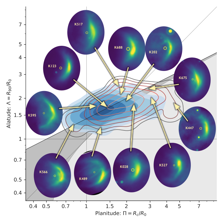
The derived bowshock shapes of all the 3-, 4-, and 5-star sources are shown in Figure 3 on the – plane, which was discussed extensively in Paper 0. Figure 3a shows each individual source with horizontal error bars that represent the dispersion of traced points from the circle fit (step 7 of the previous section) and vertical error bars that show the wing asymmetry (step 9). The horizontal error bars, which are a proxy for observational uncertainties, become very small for the 4- and 5-star sources, whereas the vertical error bars remain at roughly the level since they reflect real asymmetries in the shapes of the bow shocks.
The horizontal axis corresponds to the shape of the head of the bow shock near its apex, ranging from sharper, pointier shapes with to flatter, snubber shapes with , where it must be understood that all judgments of sharpness/flatness are with respect to the axial separation, , between the source and the bow shock apex (see Fig. 1). The vertical axis corresponds to the shape of the bow shock wings, ranging from closed “C” shapes for smaller values of to open “V” shapes for larger values of . The background shading shows the regions of the – plane occupied by simple quadric shapes (see § 4 of Paper 0): oblate spheroids (light gray), prolate spheroids (dark gray), and hyperboloids (white). The boundary between closed and open corresponds to the paraboloids, and is shown by the solid line that divides the dark gray and white regions of the graph.
In Figure 3b, we present a smoothed version of the same data. The contours show the kernel density estimator (KDE, see Leiva-Murillo & Artés-Rodríguez 2012; Scott 2015) of the two-dimensional distribution of points on the – plane. The KDE contours indicate that the distribution of 3-star sources is very similar to that of 4- and 5-star sources, although the higher-rated sources are shifted slightly to the upper right. Possible reasons for this are discussed in § 2.4 below. The bulk of the sources are concentrated around the paraboloid line, with , and . But significant minorities are found in three other regions: (1) a clump with ; (2) a vertical spur towards higher at ; and (3) a broad horizontal tail towards higher at . Thumbnail images of the emission of selected sources from different regions of the distribution are shown, in order to illustrate the range of bow shock morphologies encountered.
2.3 Correlations between non-shape parameters of the OB sources
In Figure 4 we show the distributions over all MIPSGAL bow shock sources of the bow shock size, Galactic coordinates, extinction-corrected stellar source magnitude, and dust extinction. For the bow shock size, , we use the results from our model fitting rather than the values given in the Kobulnicky et al. 2016 catalog, but the distribution is very similar, as can be seen by comparing the top-left plot of Figure 4 with Kobulnicky et al. 2016’s Figure 8.
The catalog gives the -band extinction, , derived using the method of Majewski et al. 2011. However, that assumes an intrinsic color of magnitudes, which is too red if the sources are assumed to be OB stars. We therefore re-derive from the catalog magnitudes combined with the Indebetouw et al. 2005 reddening law, but assuming magnitudes, which is more typical of early type stars. This does not make very much difference (compare the top-right plot of our Fig. 4 with Kobulnicky et al. 2016’s Fig. 9), but it does eliminate some of the apparent negative extinctions that are found in the catalog. The same reddening law gives , and this is used to derive extinction-corrected -band apparent magnitudes, .
| (a) | (b) |
|---|---|
| (a) | (b) |
|---|---|
The most significant linear correlation between any pair of parameters in Figure 4 is that between bow shock size and stellar source brightness: versus , with correlation coefficient . The distribution of depends on the absolute magnitude, , and the distance, , to the source. It is likely that variation in is the more important of the two because changes relatively little for main-sequence OB stars, ranging from (early-O) to (mid-B). This is because part of the increase in bolometric luminosity, , as one ascends the main sequence is offset by an increase in the effective temperature, , which shifts the peak of the stellar spectrum farther away from the band, resulting in , where the last step uses the upper main-sequence mass–luminosity and mass–radius scalings from Eker et al. 2015. It is true that evolved OB supergiants can be much brighter, reaching , but such stars are expected to be relatively rare. Assuming a B2V star (), then the observed range – corresponds to distances –, and the histogram peak at corresponds to , which is all perfectly reasonable.
Turning now to the distribution of bow shock angular size, , this will also be affected by distance to at least some degree, since for a constant physical size the angular size will vary as . For instance, if we assume that the physical size of all bow shocks is and the absolute magnitude of all stars is , as above, then we find the relation if is measured in arcseconds. This is shown as a dashed line on the relevant panels of Figure 4 for values of that correspond to to . It can be seen that this relation is in excellent agreement with the linear trend in the data. On the other hand, the correlation coefficient of means in broad terms that only a fraction of the total variance in is “explained” by changes in , and vice versa, implying that one or both of and is only a very imperfect proxy for . We have already seen that the spread in probably is mostly due to a spread in distance, rather than a spread in -band stellar luminosity. If this is true, it follows that it is that depends only weakly on and is more influenced by other factors.
One such factor is the stellar/environmental momentum-loss ratio, , between the two supersonic flows that form the bow shock. All other things being equal, we have for , as is typically the case. If the environment flow is constant and the OB star wind has mass-loss rate and terminal velocity , then . Empirical and theoretical studies of hot star winds (e.g., Puls et al. 1996) imply , where the final two steps apply only to main-sequence stars and again use the relations of Eker et al. 2015. If we assume as above that a B2V star with has a bow shock physical size of , and consider a sequence of stars with varying -band luminosities but all at a fixed distance of , then we find the relation . This is shown as a dotted line in the relevant panels of Figure 4 for the absolute magnitude range (O6V) to (B5V). It can be seen that this relation does not match the linear trend in the data, and predicts a much larger spread in over a narrow range in than is observed. This could mean one of two things: first, it may be that the range of stellar luminosities is significantly narrower than we have supposed, implying that B stars vastly outnumber O stars among the sources. Alternatively, there may be a positive correlation between the stellar luminosity and the momentum of the environmental flow, with the result that varies less steeply with than we have assumed. That could arise if more luminous stars were preferentially found in denser environments, or, in the case of runaways, if more luminous stars tended to be faster moving.
A third factor that may influence is the inclination, , of the bow shock axis with respect to the plane of the sky. Figure 11b of Paper 0 shows that for , then the projected becomes larger than the true as increases (see also Figs. 26 and 27 of Paper 0). It can be seen that the effect is relatively modest, with an increase in of no more than a factor of 2 to 3.
2.4 Correlation between bow shock shape and other parameters
We now investigate if the bow shock shapes of the MIPSGAL sources are correlated with any other parameters via the following methodology:
- 1.
For each of the parameters in the Kobulnicky et al. 2016 catalog, we divide the sources into two or more sub-samples, according to the value of the parameter. For quantitative parameters, such as those discussed in the previous section, we use two sub-samples of equal size, with membership determined by whether the parameter is larger or smaller than the median value. But we also use categorical parameters, such as the type of bow shock environment, or the presence/absence of emission, in which case the sub-samples are of unequal size.
- 2.
- 3.
We check if there is any statistically significant difference between the bow shock shapes of the sub-samples by applying three different non-parametric tests to and separately.
The principal test used is Kuiper’s variant of the two-sample Kolmogorov–Smirnov test (Stephens 1970; Paltani 2004, e.g.,), as implemented by the Python library function astropy.stats.kuiper_two (Astropy Collaboration et al. 2018). This is a general test of the null hypothesis that the two sub-samples are drawn from the same distribution. It returns a -value, which is the estimated probability that the observed difference between the two sub-samples would be as large as it is purely by chance if they were all were drawn from the same distribution. We consider two different thresholds for significance: (approximately 2- for a normal distribution) and (approximately 3-). We show in Appendix A that, given the large number of potential relationships that we are testing, the more stringent condition is required in order to confidently reject the null hypothesis and declare a “significant” difference between the two sub-samples, but we also consider the less strict threshold of as an indicator of “possible” difference. We supplement the general-purpose Kuiper test with two tests that probe specific features of the sample distributions: the Mann–Whitney–Wilcoxon test (Mann & Whitney 1947), which is sensitive to differences in the central value (e.g., median) and the Brown–Forsythe test (Brown & Forsythe 1974), which is sensitive to differences in the variance, or width, of the distribution (see Appendix A for details).
As shown in detail in Table 1, there is remarkably little variation in the bow shock shape distributions as a function of most of the other parameters. Two examples in which there is no significant shape difference between the sub-samples are shown in Figure 5. This lack of difference is interesting because in both examples there are a priori grounds to suspect that differences might exist. The first example (Fig. 5a) is the bow shock environment, which was categorized in Kobulnicky et al. 2016 as “Isolated” (I), “Facing a large H ii region” (FH), “Facing a bright-rimmed cloud” (FB), and “Within a giant H ii region’’ (H), and where we have merged the FH and FB categories, labelled ‘‘Facing’’ in the figure.22 2 Similar results are also found for the FB and FH categories separately. The shapes might be expected to vary with environment because the FB and FH categories should be associated with “weather vane” interactions (Povich et al. 2008) between the stellar wind and a divergent photoevaporation flow. This is expected to give a more open bow shock than in the “runaway” case of interaction of a moving star with a static environment. In the thin-shell approximation, the predicted shapes are a cantoid for weather vanes and a wilkinoid for runaways, see § 6 of Paper 0. The fact that no such difference is detected could be explained in one of two ways: (i) the momentum ratio for the weather vanes could be small, since the cantoid becomes indistinguishable from the wilkinoid as , or (ii) many of the bow shocks classified as “Isolated” might also be weather vanes rather than runaways.
The second example (Fig. 5b) divides the sources according to whether or not Kobulnicky et al. 2016 judged there to be multiple candidates for the identity of the central star that drives the bow shock. If the central star were to be misidentified in a significant number of sources, then the measured value of for those sources would be erroneous, which would increase the scatter in both and . The fact that no significant difference is seen in the shape distributions between sources with/without multiple candidates implies that such mistakes in identification of the central star must be rare.
We also tested all the other source parameters listed in Kobulnicky et al. 2016’s catalog, finding no significant shape differences for sources with/without emission, with low/high extinction, closer/farther from the Galactic plane, or closer/farther from the Galactic center. Details are given in Table 1. In all these cases, differences in mean or median less than and in less than are found, corresponding to rank biserial correlation coefficients (a non-parametric dimensionless measure of the difference between two samples, see Appendix A) of , which are not significant even at the 2- level.
The only parameters that do show a possible correlation with the bowshock shape are the bow shock angular size, , and the extinction-corrected magnitude of the central star, , which are illustrated in Figure 6. The general purpose Kuiper test indicates differences in the sub-sample distributions of at the 2- level for and at the 3- level for . It is apparent from the histograms shown in the right-hand inset graphs of Figure 6a that in the case of the small/large sub-samples it is the width rather than the central tendency of the distributions that is different, which is confirmed by the more specific Brown–Forsythe test, which indicates a difference between the sub-sample dispersions at the 3- level. In the case of the faint/bright sub-samples (Fig. 6b), it is less clear what feature of the distributions differ.
In order to investigate these effects in more detail and look for systematic trends, we divide the independent parameter ( or ) into 5 rather than 2 equal-sized sub-samples, with results in the case of shown as box plots in Figure 7. This time the -sample Anderson–Darling test (Anderson & Darling 1952; Scholz & Stephens 1987; Makarov & Simonova 2017) is used to determine the statistical significance of any observed differences. A systematic increase with in the dispersion of (upper panel of Fig. 7a) is apparent from both the interquartile range (colored boxes) and interdecile range (error bars). As a check on whether observational uncertainties might be contributing to this trend, the third and fourth rows of box plots show the statistics for, respectively, the fractional asymmetry of the bowshock wings and the standard deviation, , of the individual points on the bow shock that go into determining (see step 8 of the tracing/fitting methodology described in § 2.1). It can be seen that neither of these quantities tends to increase with , and in fact there is a significant decrease in with . This implies that the increase with angular size of the diversity of bow shock wing shapes is real, and not due to observational uncertainties. On the other hand, we find that no clear trends are evident as a function of source magnitude (not illustrated), which leads us to suspect that the result obtained for the 2-sample Kuiper test was a false positive, as is also supported by the analysis in Appendix A and Figure 14.
As mentioned in § 2.2 there is also a shape difference between the 3-star sources and the 4/5-star sources (see Fig. 3b). The -values of statistical tests (see Table 1) indicate that this is much more significant than any correlation with the other parameters discussed in this section ( for and for ). This means that it cannot be simply due to the tendency of the higher-rated sources to have larger angular sizes. However, the subjective nature of the star ratings makes this result hard to interpret.
3 Far-infrared arcs around late-type stars
| (a) | (b) |
 |
 |
| (c) | (d) |
 |
 |
| (e) | (f) |
 |
 |
| (g) | (h) |
 |
 |
| (a) | (b) |
 |
 |
| (c) | (d) |
 |
 |
| (e) | (f) |
 |
 |
| (g) | (h) |
 |
 |
We obtain a second sample of bow shocks from a far-infrared survey (Cox et al. 2012) of circumstellar shells around known asymptotic giant branch (AGB) stars and cool supergiants, obtained as part of the Herschel MESS (Mass-loss of Evolved StarS) program (Groenewegen et al. 2011). The survey sources were divided into four classes by Cox et al. 2012, according to the overall shape of the extended emission at (see their Table 4): “fermata \setlines10\smallmusicsize\nobarnumbers\nostartrule\staffbotmarg0pt \setclefsymbol1\clef@skip0pt \startextract\addspace-\afterruleskip \notes\fermataup-2\en\zendextract”, or arcs (Class I); “eyes ” (Class II); “rings ” (Class III), and “irregular ¸” (Class IV). Of these, only the Class I sources clearly correspond to bow shocks, which represent 22 out of 50 total sources detected with extended emission. For our sample, we select the 16 Class I sources where the shape parameters can be reliably measured, and which are shown in Figures 8 and 9. The remaining six Class I sources (Fig. 1 of Cox et al. 2012) are too asymmetrical or irregular to reliably determine and , and are therefore excluded from our sample.
In most sources, the bow shock shell is most clearly visible in the band, with the exception being CW Leo where the band is used instead. In several sources, the shell is split into multiple filaments, with the clearest example being Ori (Betelgeuse), shown in Figure 8(a). For such sources, we take the outer envelope of the filaments as the bow shock arc. Given this complication, and the fact that the angular resolution relative to the bow shock size is much better than in the MIPSGAL sources, we judge that the arc tracing is best performed by eye and this is carried out using the SAOImage DS9 FITS viewer (Joye & Mandel 2003), with results shown as small red open circles in Figures 8 and 9 (more details of this technique are given in §§ 6 and 7 of Paper 0). Subsequently, the bow shock parameters , , and are determined by circle fits, as in steps 5–9 of § 2.1, with results shown in magenta on the figures.
Figure 10 compares the distributions of bow shock shapes between the Herschel (RSG/AGB) and MIGSGAL (OB star) samples. The Kuiper test gives a highly significant difference between the distributions of the two samples, but only a marginally significant difference between the distributions (detailed results are shown in Table 1). The Herschel sources show considerably smaller alatude (median ), implying bow shock wings that are more closed than in the MIPSGAL sources (median ). For the planitude, there is only a slight difference in average values: median for Herschel versus for MIPSGAL, which is not statistically significant (rank biserial ). On the other hand, the dispersion in is four times smaller for the Herschel sample, which is marginally significant (Brown–Forsythe ). In particular, the MIPSGAL sample shows a substantial minority of very flat-nosed shapes (), but these are absent in the Herschel sample. The same can be seen directly by comparing the RSG/AGB bow shock shapes in Figures 8 and 9 with the representative OB bow shocks of Figure 3b. The MIPSGAL sources K489 and K123 have shapes that are similar to specific Herschel sources (UU Aur and R Hya, respectively), while sources such as K447 (extreme flat head) or K517 (extreme open wings) have no analog among the Herschel sources.
4 Stationary emission line arcs in M42

We obtain a third sample of bow shocks from a catalog of stationary emission line arcs in the Orion Nebula (Bally et al. 2000), which are detected via their H emission in HST ACS surveys of the nebula (Bally et al. 2006; Robberto et al. 2013). Out of a total of 73 such objects (Gutiérrez-Soto 2015) we have selected 18 where the observations are of sufficient quality to reliably measure the planitude and alatude. Images in the ACS f658n filter of these sources are shown in Figure 11. Some of the sources were identified as LL Orionis-type objects by Bally & Reipurth 2001 and are identified as LL 1–6. The remaining sources are labeled by their coordinate-based designation according to the system of O’Dell & Wen 1994. The determination of the bow shock shape for each source was carried out as described in § 7 of Paper 0, using the “ridge” method for manually tracing the arc (see Fig. 28 of Paper 0). In some sources, such as LL 1, LL 6, 109–246, and 4468–605, a high-velocity jet flow is also seen to issue from the star (Bally et al. 2006; Henney et al. 2013). We took care when tracing the arcs of such sources to avoid regions where jet knot emission is projected on the bow shock shell.
The planitude and alatude are found by circle fitting using the algorithm described in Paper 0’s Appendix E, as implemented in the python program circle-fit.py.33 3 https://github.com/div-B-equals-0/circle-fit The only adjustable parameter of the algorithm is , the maximum angle from the bow shock axis of points that are included in the circle fit. We tested all values of in increments from to and found that to gives stable results for all sources. The accuracy of the fitted planitudes can be estimated from the dispersion in values of for the same source with different , which we find to be . The fitted alatudes have a much smaller dispersion , but in this case the accuracy is limited by the asymmetry of the wings, as characterized by with an RMS value of .
The resultant shape distribution for the Orion Nebula arcs is shown in Figure 12, where it is compared with the OB star shapes from § 2.2. It can be seen that both the planitude and alatude distributions are shifted towards higher values, with median values of and . The difference from the MIPSGAL sources ( and ) is highly statistically significant, as indicated by extremely low -values for the Kuiper tests. It is also at least 4 times larger than the systematic fitting uncertainties discussed in the previous paragraph. On closer inspection, it appears that the shape distribution is bimodal. Four of the sources (005–514, 4468–605, 116–3101, 308–3036) are similar to typical OB stars, with , whereas the remainder are concentrated in the range to , with an extended tail towards higher planitude. The alatudes mainly follow the line for parabolas, (see App. C of Paper 0), and the deviations from this line can be readily understood in terms of peculiar morphologies of the source (Fig. 11). For instance, LL 4 and 266–558 both show large alatudes for their respective planitudes and these are both sources where the bow shock wings seem to bend outwards instead of following the curve from the apex region. In contrast, 030–524 has a small alatude for its planitude and this is a very asymmetric source with an apparent corner to the shell on one side.
Uniquely among the three bow shock datasets, for the Orion Nebula arcs we know the source of the external flow. This is not the stellar wind from the high-mass stars at the center of the cluster, which has insufficient momentum at the position of the arcs (Bally et al. 2000), nor is it due to stars’ own motions, since the space velocities of all these sources are very low, conforming to the velocity dispersion of the Orion Nebular Cluster (Dzib et al. 2017; Kim et al. 2018). Instead it is due to the transonic champagne flow of photoionized gas away from the core of the nebula (Zuckerman 1973; Henney et al. 2005), which has its density peak in the Orion S region (Weilbacher et al. 2015), located roughly SW of the dominant Trapezium star Ori C. The bow shock sources are located at much larger distances of to from Ori C, so that the ratio can be used as a proxy for the local divergence of the champagne flow on the scale of the bow shock (notice that the symmetry axes of the bow shocks in Fig. 11 are always roughly parallel to the direction to Ori C). This is indicated by the color of the points in Figure 12, with lighter colors corresponding to a larger and hence a more divergent external flow. It can be seen that there is some correlation between the bow shock shapes and : the source with the largest , 109–246, also has the largest , while the four sources with low and all have low . However, the correlation is far from perfect, with a Pearson correlation coefficient of only .
5 Discussion
In this section, we discuss the physical implications of our empirical findings regarding bow shock shapes. Our most reliable result is the average shape of the OB bow shocks from the 227 MIPSGAL sources with quality rating of 3 stars or higher. This yields mean values of and , or median values of and . The uncertainty quoted on the mean values is the “standard error of the mean”: , where is the rms dispersion and is the number of sources. Note that in the case of the planitude is considerably smaller than , so the latter would be a more conservative estimate of the uncertainty.44 4 This is because the distribution of is approximately log-normal, which yields a significant tail towards high values when converted to linear space. These values can be compared with the predictions of the thin-shell wilkinoid model (Wilkin 1996), which are , when the bow shock axis lies in the plane of the sky (following Paper 0, this is defined as the zero point of the inclination angle, ). When the axis is inclined, both planitude and alatude are predicted to decrease but not by very much, tending to , as (see § 5.3 of Paper 0). The median observed value falls squarely inside this range for both the planitude and alatude, which is a remarkable triumph for the Wilkin 1996 model.
5.1 Diversity in bow shock shapes
On the other hand, turning now to the variety of bow shock shapes, we see that the wilkinoid can no longer explain our results. The rms dispersions of the planitude and alatude distributions for the MIPSGAL sources are and (Tab. 1), which are respectively 5 times and 3 times larger than the total range of variation of and predicted for the wilkinoid surface. Although some of the dispersion is due to uncertainties in the observations and the fitting algorithm, this contribution is expected to be small, especially for the larger, well-resolved sources, for which systematic uncertainties in the methods for determining and will dominate. Conservative upper limits to the relative size of these uncertainties were estimated in § 7 of Paper 0 to be for and for , whereas the observed dispersions are roughly twice as large: and . Furthermore, the variations in planitude and alatude are readily apparent by eye, as is demonstrated by the example bow shock images shown in Figure 3b. Sources such as K123 have very typical shapes and fall near the center of the – distribution, whereas high- sources such as K447 have a very flat apex region, while low- sources such as K566 have a pointier, almost triangular apex. High- sources, such as K517, have very open wings that bend away from the star, while low- sources such as K489 have closed wings and a semi-circular appearance.
5.1.1 The influence of projection effects
In Paper 0 we found that certain bow shock shapes can show a much greater variation in their projected appearance as a function of inclination angle than is seen for the wilkinoid. For example, the cantoids and ancantoids, which have asymptotically hyperbolic far wings, can shift towards higher apparent planitude and alatude as the inclination increases, generally with (Fig. 20 of Paper 0). This might plausibly explain the vertical spur towards higher seen in the empirical distribution (§ 2.2). A different behavior is shown by bow shocks with very flat apex regions, such as the MHD simulation from Meyer et al. 2017 that is analyzed in the § 6 of Paper 0. This shows a high planitude when the orientation is exactly edge-on, but decreases sharply along a roughly horizontal track as the inclination increases (Fig. 25 of Paper 0). This is similar to the principal axis of variation of the observed shapes (e.g., Fig. 3a).
If such variations in orientation do make a significant contribution to the observed distribution of bow shock shapes in the - plane, then various predictions follow, which might be observationally tested. High-planitude sources with would be expected to have low inclinations, , whereas high-alatude sources with would be expected to have high inclinations, . Unfortunately, determination of the inclination for individual sources requires high resolution spectroscopy of emission lines in order to map the kinematics of the flow in the bow shock shell (Henney et al. 2013, e.g.,). This is not currently available for the majority of the MIPSGAL sources, which are detected only by their dust continuum emission. A further prediction for the high-alatude sources is that the environmental flow should be divergent rather than plane-parallel, in order to give a cantoid shape instead of a wilkinoid. This would tend to favor “weather-vane” cases, where the interstellar medium is flowing past the star, and disfavor “runaway” cases, where the star is moving through a static medium. However, in § 2.4 we found no significant difference in the shape distributions as a function of the bow shock environment. Figure 5a shows that the alatudes of sources that are facing H ii regions or bright-rimmed clouds (and therefore might be expected to be immersed in a champagne flow) are no higher than sources that are isolated.
5.1.2 Perturbations to the bow shape
(a)
(b)
An alternative explanation for the variety of observed bow shock shapes is that they are due to time-dependent perturbations to an underlying base shape. For instance, multiple studies have shown that stellar bow shock shells can be unstable (Dgani et al. 1996a; Dgani et al. 1996b; Blondin & Koerwer 1998; Comeron & Kaper 1998; Meyer et al. 2014a), leading to large amplitude oscillations in the shell shape. The oscillations are found to be most vigorous when the post shock cooling is highly efficient, allowing the formation of a thin shell (see Paper I). Even in cases where the shell is stable, oscillations may be driven by periodic variations in the stellar wind mass-loss rate or velocity, or by inhomogeneities in the ambient stream. Rather than using a particular dynamical model of these oscillations, we instead crudely simulate their effect by assuming a constant amplitude standing wave perturbation to the base shape, as described in Appendix B. Example results are shown in Figure 13 for an ensemble of bow shocks with different orientations and phases of oscillation, considering three different underlying base shapes. It can be seen that modest amplitudes of 10 to 20% can give rise to a distribution in and similar to that observed for the MIPSGAL sources when the oscillation wavelength is of the same order as the bow shock size.
An attractive feature of the oscillation hypothesis is that it naturally explains why we find little correlation between the bow shock shape and other source parameters (§ 2.4), since the instantaneous shape at any instant is largely a matter of chance rather than being due to any intrinsic property of the source. The one significant correlation that we do find is that the alatude distribution is broader for bow shocks with larger angular sizes. This might be explained if the relative amplitude of oscillations were higher for sources with more powerful winds. Meyer et al. 2016 in their Fig. 2 plot the “axis ratio” (which is our ) as a function of apex distance for a large set of hydrodynamic bow shock simulations. They find the most unstable bow shocks (with the largest spread in ) to be those associated with the highest mass stars in a relatively dense medium, which have apex distances of . This corresponds to for distances less than , which is larger than the median angular size for the MIPSGAL sources, making this a plausible explanation for our statistical result.
5.2 Variations between different source classes
We now address the difference in shape distribution between the different classes of source. Compared with the OB star bow shocks, the cool star sample from Cox et al. 201255 5 Three of these sources are high-mass red supergiant (RSG) stars, while the remaining 13 are intermediate-mass asymptotic giant branch (AGB) stars. shows a significantly smaller alatude of (see Fig. 10).66 6 Although the planitude also appears to be slightly smaller, this is not very statistically significant due to the small number of cool star sources and the large width of the OB star planitude distribution. Such a closed shape for the wings is inconsistent with the wilkinoid value of , which is surprising given that the emission shells in these sources are relatively narrow (Figs. 8 and 9), so one might have thought that the thin-shell approximation of Wilkin 1996 would be more appropriate than for the OB stars, but this is clearly not the case. One possible explanation for this might be that the bow shocks have not had time to reach a steady-state configuration, as was suggested by Mohamed et al. 2012 for the case of Ori. The dynamical timescales, , for the cool star bow shocks are of order and numerical simulations e.g., Fig. 11 of Mohamed et al. 2012 and Fig. 2 of van Marle et al. 2014 show that the bow shock wings take of order to fully unfold. However, this is still short compared with typical RSG and AGB lifetimes, so while it might apply to a single source it does not work as an explanation for an entire class of sources, especially given that the alatude and planitude distributions for these sources are so narrow (Fig. 10). A more promising explanation is that the shape difference reflects a different origin for the infrared-emitting dust. In hot stars, the stellar wind is dust-free, so the only dust shell comes from the interstellar medium and lies outside the astropause (contact discontinuity). In cool stars, the stellar wind is also dusty, which could give rise to significant infrared emission from near the stellar wind’s termination shock, as has been found from hydrodynamic simulations (Meyer et al. 2014b). This is certainly the case for at least one of our cool star sources, the C-AGB star CW Leo (IRC+10216), where ultraviolet GALEX observations (Sahai & Chronopoulos 2010) clearly show both the outer shock and the wind termination shock, and comparison with the Herschel images demonstrate that the infrared dust emission is associated with the latter.
In the case of the Orion Nebula bow shocks (§ 4), we have the opposite situation, where the alatude and planitude are both significantly larger on average than for the OB star sources (Fig. 12). On the face of it, this is surprising because there are two differences between the source classes that would tend to work in the other direction. First, many of the Orion sources are proplyds, or externally illuminated photoevaporating disks (O’Dell et al. 2008), in which the inner wind is not isotropic but instead is mildly concentrated towards the symmetry axis (García-Arredondo et al. 2001), so that simple models predict an ancantoid shape (Tarango-Yong & Henney 2018, § 5) that is less open than for an isotropic wind. Second, as was the case with the cool star sources, both the shocked inner wind and the shocked outer stream are expected to contribute to the emission arcs. Indeed, in several of the sources of Figure 11 (LL 3, 116–3101, 266-558, 308-3036, and LL 5), a two-component emission structure is apparent. In the case of the cool star bow shocks, we invoked this as a possible explanation of their low alatude (see previous paragraph), so some stronger countervailing factor is necessary in order to explain why the opposite is seen in the Orion Nebula bow shocks.
Four possible origins for this countervailing factor suggest themselves: (i) the external flow may be more divergent in the Orion sources; (ii) the Mach number of the external flow may be systematically lower; (iii) the fact that the arcs are observed in recombination line emission instead of dust continuum may cause different observational biases; (iv) the shapes may be influenced by collimated jet outflows from the young stars. We now address each of these in turn.
In case (i) one would expect and to be positively correlated with , where is the bow shock size (star–apex separation) and is the distance from the center of divergence of the external flow. In § 4 we found that these are indeed correlated, but only weakly. A more serious objection to this idea is that according to hypersonic thin-shell models (Canto et al. 1996) the momentum ratio parameter must be relatively large in order to give significantly open bow shock shapes. From Figure 20 of Paper 0 we see that is required in order to give . However, for small one has , which yields to for our sources, so that divergence ought to have little effect on the shapes.
Case (ii) arises from the fact that, if the hypersonic assumption is relaxed, then the opening angle between the outer bow shock and the contact discontinuity in the wings becomes increasingly large as the Mach number, , drops towards unity. This is a consequence of the shock polar relation for oblique shocks (Landau & Lifshitz 1987, §§ 92 and 113) and applies to both the radiative and non-radiative case. It will tend to produce more open shapes, at least in the case that the emission is dominated by the outer shell. At the same time, the relative thickness of the shell, , is predicted to increase as decreases . We have therefore measured for the Orion sources, finding values ranging from with median of . We have not measured for the full MIPSGAL sample, but Figure 11 of Paper III gives the values for the sub-sample of OB bow shocks studied by (Kobulnicky et al. 2018). The median value is 0.2, implying thinner shells than in the Orion Nebula bow shocks, which lends support to the idea that the Mach number may be lower in the latter. However, among the Orion sources we find that is completely uncorrelated with either or ( and , respectively).
Case (iii) attempts to explain the difference in shapes as a result of an “optical illusion” whereby the OB star bow shocks are in reality more open than they appear. The hydrogen recombination line surface brightness from an isothermal shell is proportional to the emission measure (line of sight integral of the product of proton and electron densities), whereas the mid-infrared surface brightness is not simply proportional to the dust column density, since it results from the reprocessing of stellar radiation. For typical bow shock grain temperatures to , Kobulnicky et al. 2017 the band used for the OB star sample lies on the short wavelength Wien side of the dust emission spectrum, which gives a very steep radial dependence of the emissivity. Acreman et al. 2016 calculate synthetic emission maps from hydrodynamical simulations and show that, even for a relatively thin bow shock shell, the emission arc seen in H tends to be more open than the arc seen in the mid-infrared (see their Fig. 3). The effect should be even larger for thicker shells, as demonstrated by Mackey et al. 2016, who simulate the subsonic motion of an O star through its H ii region and show that this can give rise to an apparent bow shock at even when there is no corresponding dense shell at all.
Finally, case (iv) arises from the observation that several of the Orion sources possess high velocity () collimated jets (Bally et al. 2006), which produce strings of emission knots that partially overlap the wings of the bow shock. In the case of 109–246, LL 1, LL 4, LL 5, and LL 6, the projected jet axis is roughly perpendicular to the projected bow shock axis, and two of these (109–246 and LL 6) have the most extreme high values of and . There are several other Orion Nebula bow shock sources with perpendicular jets (LL 2, 203–3039, 261–3018, 344–3020, and LL 7), which we omitted from our sample because of difficulty in measuring , but the majority also have large planitudes . Only one source, 4468–605, has a jet oriented parallel to the bow shock axis, and this has the smallest and third-smallest of the sample. The circumstantial evidence thus points towards the jets playing some role in shaping the bow shocks when they are oriented perpendicular to the axis, even though we took care when tracing the bow shock ridges to avoid any region with superimposed jet knots. This would break the cylindrical symmetry of the bow shock, which should have a kinematic signature. However, in the only two sources that have been studied kinematically (Henney et al. 2013), the bow shock shell does not show any sign of the red/blue asymmetry that is seen in the jet knots, which argues against any such association.
6 Summary
We have presented a statistical study of the shapes of three different classes of stellar bow shocks, as characterized by their flatness of apex (planitude, ) and openness of wings (alatude, ), following the terminology of Tarango-Yong & Henney 2018. Our principal findings are as follows:
- 1.
Bow shocks driven by hot OB stars, from the mid-infrared catalog of Kobulnicky et al. 2016, have an average shape that is consistent with predictions of the Wilkin 1996 analytic model, but the dispersion in observed shapes is many times larger than predicted by that model.
- 2.
The bow shock shapes show little correlation with other parameters of the source, such as stellar magnitude, Galactic latitude or longitude, extinction, or type of environment (cluster versus isolated). The only exception is that the dispersion in alatude is higher for bow shocks of larger angular size.
- 3.
A possible explanation for the previous results is that the variation in shapes is caused by time dependent oscillations in the bow shock surface, with relative amplitude of 10 to 20% and wavelength of order the bow shock size. The oscillations may either be due to dynamic instabilities in the bow shock shell or be driven by temporal variations in the stellar wind. If the oscillations were more vigorous for stars with more powerful winds, it could explain the correlation with angular size.
- 4.
Bow shocks driven by cool luminous stars (red supergiants and asymptotic giant branch stars), from the catalog of (Cox et al. 2012), have an average shape , which has a significantly smaller alatude than the OB star sources, and which is not consistent with the Wilkin 1996 model. We suggest that this may be due to their dust emission being dominated by shocked stellar wind material, instead of shocked ambient material as is the case with the OB stars.
- 5.
Bow shocks driven by proplyds and other young stars in the outer regions of the Orion Nebula, from the catalogs of Bally et al. 2006 and Gutiérrez-Soto 2015, have an average shape of , with a significant tail up to . A minority of these sources () have shapes similar to the OB star bow shocks, but the remainder have much flatter apexes and more open wings. We suggest several possible mechanisms to explain this difference: divergent ambient flow; low Mach number; observational biases; influence of collimated jets, but the available evidence for and against each of these is mixed.
Acknowledgements
We are grateful for financial support provided by Dirección General de Asuntos del Personal Académico, Universidad Nacional Autónoma de México, through grants Programa de Apoyo a Proyectos de Investigación e Inovación Tecnológica IN111215 and IN107019.
References
- Acreman et al. (2016) Acreman D. M., Stevens I. R., Harries T. J., 2016, MNRAS, 456, 136
- Anderson & Darling (1952) Anderson T. W., Darling D. A., 1952, Ann. Math. Statist., 23, 193
- Arthur & Hoare (2006) Arthur S. J., Hoare M. G., 2006, ApJS, 165, 283
- Astropy Collaboration et al. (2018) Astropy Collaboration et al., 2018, AJ, 156, 123
- Bally & Reipurth (2001) Bally J., Reipurth B., 2001, ApJ, 546, 299
- Bally et al. (1998) Bally J., Sutherland R. S., Devine D., Johnstone D., 1998, AJ, 116, 293
- Bally et al. (2000) Bally J., O’Dell C. R., McCaughrean M. J., 2000, AJ, 119, 2919
- Bally et al. (2006) Bally J., Licht D., Smith N., Walawender J., 2006, AJ, 131, 473
- Baranov et al. (1970) Baranov V. B., Krasnobaev K. V., Kulikovskii A. G., 1970, Akademiia Nauk SSSR Doklady, 194, 41
- Baranov et al. (1971) Baranov V. B., Krasnobaev K. V., Kulikovskii A. G., 1971, Soviet Physics Doklady, 15, 791
- Benaglia et al. (2010) Benaglia P., Romero G. E., Martí J., Peri C. S., Araudo A. T., 2010, A&A, 517, L10
- Blondin & Koerwer (1998) Blondin J. M., Koerwer J. F., 1998, New Astron., 3, 571
- Bodensteiner et al. (2018) Bodensteiner J., Baade D., Greiner J., Langer N., 2018, A&A, 618, A110
- Brown & Bomans (2005) Brown D., Bomans D. J., 2005, A&A, 439, 183
- Brown & Forsythe (1974) Brown M. B., Forsythe A. B., 1974, Journal of the American Statistical Association, 69, 364
- Brownsberger & Romani (2014) Brownsberger S., Romani R. W., 2014, ApJ, 784, 154
- Canto et al. (1996) Canto J., Raga A. C., Wilkin F. P., 1996, ApJ, 469, 729
- Carey et al. (2009) Carey S. J., et al., 2009, PASP, 121, 76
- Comeron & Kaper (1998) Comeron F., Kaper L., 1998, A&A, 338, 273
- Cox et al. (2012) Cox N. L. J., et al., 2012, A&A, 537, A35
- Cureton (1956) Cureton E. E., 1956, Psychometrika, 21, 287
- Cyganowski et al. (2003) Cyganowski C. J., Reid M. J., Fish V. L., Ho P. T. P., 2003, ApJ, 596, 344
- Dgani et al. (1996a) Dgani R., van Buren D., Noriega-Crespo A., 1996a, ApJ, 461, 372
- Dgani et al. (1996b) Dgani R., van Buren D., Noriega-Crespo A., 1996b, ApJ, 461, 927
- Dyson & de Vries (1972) Dyson J. E., de Vries J., 1972, A&A, 20, 223
- Dzib et al. (2017) Dzib S. A., et al., 2017, ApJ, 834, 139
- Eker et al. (2015) Eker Z., et al., 2015, AJ, 149, 131
- García-Arredondo et al. (2001) García-Arredondo F., Henney W. J., Arthur S. J., 2001, ApJ, 561, 830
- Geballe et al. (2004) Geballe T. R., Rigaut F., Roy J.-R., Draine B. T., 2004, ApJ, 602, 770
- Groenewegen et al. (2011) Groenewegen M. A. T., et al., 2011, A&A, 526, A162
- Gull & Sofia (1979) Gull T. R., Sofia S., 1979, ApJ, 230, 782
- Gutiérrez-Soto (2015) Gutiérrez-Soto L. Á., 2015, Master’s thesis, Universidad Nacional Autónoma de México
- Gvaramadze & Bomans (2008) Gvaramadze V. V., Bomans D. J., 2008, A&A, 490, 1071
- Hayward et al. (1994) Hayward T. L., Houck J. R., Miles J. W., 1994, ApJ, 433, 157
- Head et al. (2015) Head M. L., Holman L., Lanfear R., Kahn A. T., Jennions M. D., 2015, PLOS Biology, 13, 1
- Henney & Arthur (2019a) Henney W. J., Arthur S. J., 2019a, MNRAS, 486, 3423 (Paper I)
- Henney & Arthur (2019b) Henney W. J., Arthur S. J., 2019b, MNRAS, 486, 4423 (Paper II)
- Henney & Arthur (2019c) Henney W. J., Arthur S. J., 2019c, arXiv e-prints, 1904.00343 MNRAS submitted (Paper III)
- Henney et al. (2005) Henney W. J., Arthur S. J., García-Díaz M. T., 2005, ApJ, 627, 813
- Henney et al. (2013) Henney W. J., García-Díaz M. T., O’Dell C. R., Rubin R. H., 2013, MNRAS, 428, 691
- Immer et al. (2014) Immer K., Cyganowski C., Reid M. J., Menten K. M., 2014, A&A, 563, A39
- Indebetouw et al. (2005) Indebetouw R., et al., 2005, ApJ, 619, 931
- Johnstone et al. (1998) Johnstone D., Hollenbach D., Bally J., 1998, ApJ, 499, 758
- Joye & Mandel (2003) Joye W. A., Mandel E., 2003, in Payne H. E., Jedrzejewski R. I., Hook R. N., eds, Astronomical Society of the Pacific Conference Series Vol. 295, Astronomical Data Analysis Software and Systems XII. p. 489
- Kim et al. (2018) Kim D., Lu J. R., Konopacky Q., Chu L., Toller E., Anderson J., Theissen C. A., Morris M. R., 2018, arXiv e-prints
- Klaassen et al. (2018) Klaassen P. D., et al., 2018, A&A, 611, A99
- Kobulnicky et al. (2010) Kobulnicky H. A., Gilbert I. J., Kiminki D. C., 2010, ApJ, 710, 549
- Kobulnicky et al. (2016) Kobulnicky H. A., et al., 2016, ApJS, 227, 18
- Kobulnicky et al. (2017) Kobulnicky H. A., Schurhammer D. P., Baldwin D. J., Chick W. T., Dixon D. M., Lee D., Povich M. S., 2017, AJ, 154, 201
- Kobulnicky et al. (2018) Kobulnicky H. A., Chick W. T., Povich M. S., 2018, ApJ, 856, 74 (K18)
- Kulkarni & Hester (1988) Kulkarni S. R., Hester J. J., 1988, Nature, 335, 801
- Landau & Lifshitz (1987) Landau L. D., Lifshitz E. M., 1987, Fluid Mechanics, Second Edition: Volume 6 (Course of Theoretical Physics), 2 edn. Course of theoretical physics / by L. D. Landau and E. M. Lifshitz, Vol. 6, Butterworth-Heinemann
- Leiva-Murillo & Artés-Rodríguez (2012) Leiva-Murillo J. M., Artés-Rodríguez A., 2012, Pattern Recogn. Lett., 33, 1717
- Mac Low et al. (1991) Mac Low M.-M., van Buren D., Wood D. O. S., Churchwell E., 1991, ApJ, 369, 395
- Mackey et al. (2015) Mackey J., Gvaramadze V. V., Mohamed S., Langer N., 2015, A&A, 573, A10
- Mackey et al. (2016) Mackey J., Haworth T. J., Gvaramadze V. V., Mohamed S., Langer N., Harries T. J., 2016, A&A, 586, A114
- Majewski et al. (2011) Majewski S. R., Zasowski G., Nidever D. L., 2011, ApJ, 739, 25
- Makarov & Simonova (2017) Makarov A. A., Simonova G. I., 2017, Journal of Mathematical Sciences, 221, 580
- Mann & Whitney (1947) Mann H. B., Whitney D. R., 1947, The Annals of Mathematical Statistics, 18, 50
- Meyer et al. (2014a) Meyer D. M.-A., Gvaramadze V. V., Langer N., Mackey J., Boumis P., Mohamed S., 2014a, MNRAS, 439, L41
- Meyer et al. (2014b) Meyer D. M.-A., Mackey J., Langer N., Gvaramadze V. V., Mignone A., Izzard R. G., Kaper L., 2014b, MNRAS, 444, 2754
- Meyer et al. (2016) Meyer D. M.-A., van Marle A.-J., Kuiper R., Kley W., 2016, MNRAS, 459, 1146
- Meyer et al. (2017) Meyer D. M.-A., Mignone A., Kuiper R., Raga A. C., Kley W., 2017, MNRAS, 464, 3229
- Mohamed et al. (2012) Mohamed S., Mackey J., Langer N., 2012, A&A, 541, A1
- Noriega-Crespo et al. (1997) Noriega-Crespo A., van Buren D., Dgani R., 1997, AJ, 113, 780
- O’Dell (2001) O’Dell C. R., 2001, AJ, 122, 2662
- O’Dell & Wen (1994) O’Dell C. R., Wen Z., 1994, ApJ, 436, 194
- O’Dell et al. (1993) O’Dell C. R., Wen Z., Hu X., 1993, ApJ, 410, 696
- O’Dell et al. (2008) O’Dell C. R., Muench A., Smith N., Zapata L., 2008, Star Formation in the Orion Nebula II: Gas, Dust, Proplyds and Outflows. p. 544
- Paltani (2004) Paltani S., 2004, A&A, 420, 789
- Peri et al. (2012) Peri C. S., Benaglia P., Brookes D. P., Stevens I. R., Isequilla N. L., 2012, A&A, 538, A108
- Peri et al. (2015) Peri C. S., Benaglia P., Isequilla N. L., 2015, A&A, 578, A45
- Pikel’ner (1968) Pikel’ner S. B., 1968, Astrophys. Lett., 2, 97
- Povich et al. (2008) Povich M. S., Benjamin R. A., Whitney B. A., Babler B. L., Indebetouw R., Meade M. R., Churchwell E., 2008, ApJ, 689, 242
- Puls et al. (1996) Puls J., et al., 1996, A&A, 305, 171
- Reid & Ho (1985) Reid M. J., Ho P. T. P., 1985, ApJ, 288, L17
- Robberto et al. (2005) Robberto M., et al., 2005, AJ, 129, 1534
- Robberto et al. (2013) Robberto M., et al., 2013, ApJS, 207, 10
- Sahai & Chronopoulos (2010) Sahai R., Chronopoulos C. K., 2010, ApJ, 711, L53
- Sahai et al. (2012) Sahai R., Güsten R., Morris M. R., 2012, ApJ, 761, L21
- Sanchez-Bermudez et al. (2014) Sanchez-Bermudez J., Schödel R., Alberdi A., Muzić K., Hummel C. A., Pott J.-U., 2014, A&A, 567, A21
- Scholz & Stephens (1987) Scholz F. W., Stephens M. A., 1987, Journal of the American Statistical Association, 82, 918
- Scott (2015) Scott D. W., 2015, Multivariate density estimation: theory, practice, and visualization, 2nd edn. John Wiley & Sons
- Sexton et al. (2015) Sexton R. O., Povich M. S., Smith N., Babler B. L., Meade M. R., Rudolph A. L., 2015, MNRAS, 446, 1047
- Smith et al. (2005) Smith N., Bally J., Shuping R. Y., Morris M., Kassis M., 2005, AJ, 130, 1763
- Steggles et al. (2017) Steggles H. G., Hoare M. G., Pittard J. M., 2017, MNRAS, 466, 4573
- Stephens (1970) Stephens M. A., 1970, Journal of the Royal Statistical Society. Series B (Methodological), 32, 115
- Tanner et al. (2005) Tanner A., Ghez A. M., Morris M. R., Christou J. C., 2005, ApJ, 624, 742
- Tarango-Yong & Henney (2018) Tarango-Yong J. A., Henney W. J., 2018, MNRAS, 477, 2431 (Paper 0)
- Ueta et al. (2006) Ueta T., et al., 2006, ApJ, 648, L39
- Ueta et al. (2008) Ueta T., et al., 2008, PASJ, 60, S407
- Weilbacher et al. (2015) Weilbacher P. M., et al., 2015, A&A, 582, A114
- Werner et al. (2004) Werner M. W., et al., 2004, ApJS, 154, 1
- Wilkin (1996) Wilkin F. P., 1996, ApJ, 459, L31
- Wood & Churchwell (1989) Wood D. O. S., Churchwell E., 1989, ApJS, 69, 831
- Wright et al. (2010) Wright E. L., et al., 2010, AJ, 140, 1868
- Zuckerman (1973) Zuckerman B., 1973, ApJ, 183, 863
- van Buren & McCray (1988) van Buren D., McCray R., 1988, ApJ, 329, L93
- van Buren et al. (1990) van Buren D., Mac Low M.-M., Wood D. O. S., Churchwell E., 1990, ApJ, 353, 570
- van Buren et al. (1995) van Buren D., Noriega-Crespo A., Dgani R., 1995, AJ, 110, 2914
- van Marle et al. (2014) van Marle A. J., Decin L., Meliani Z., 2014, A&A, 561, A152
Appendix A Distribution of p-values for all correlations tested
(a)
(b)
| Dependent | Mean | Std. Dev. | Obs. Disp. | .Effect sizes. | Non-parametric test -values | ||||||||
| Comparison | Variable | Cohen | K–S | Rank | B–F | ||||||||
| (1) | (2) | (3) | (4) | (5) | (6) | (7) | (8) | (9) | (10) | (11) | (12) | (13) | (14) |
| Median split of continuous independent variables | |||||||||||||
| Faint/bright | 1.654 | 0.0335 | |||||||||||
| magnitude | 0.174 | 0.308 | 0.018 | 0.0235 | |||||||||
| Low/high | |||||||||||||
| bow shock size, | 1.342 | 0.00208 | 0.00139 | ||||||||||
| 0.00612 | |||||||||||||
| Low/high | |||||||||||||
| extinction, | |||||||||||||
| Low/high | 0.0379 | ||||||||||||
| High/low | |||||||||||||
| Categorical independent variables | |||||||||||||
| Environment: | |||||||||||||
| Isolated vs Facing | |||||||||||||
| Environment: | |||||||||||||
| Isolated vs H ii | |||||||||||||
| Single/multiple | |||||||||||||
| source candidate | |||||||||||||
| With/without | |||||||||||||
| emission | |||||||||||||
| 3-star vs (4+5)-star | 0.386 | 0.431 | 3.75e-05 | 7.66e-07 | |||||||||
| 0.328 | 0.525 | 0.000562 | 2.63e-05 | ||||||||||
| Intercomparison with other datasets | |||||||||||||
| MIPS vs Orion | 0.57 | 1.37 | 1.911 | 0.00112 | 5.73e-05 | 0.00133 | |||||||
| 0.71 | 2.308 | 2.526 | 9.99e-06 | 5.49e-07 | 1.49e-09 | ||||||||
| 0.642 | 2.243 | 3.173 | 7.14e-06 | 5.95e-06 | 1.07e-10 | ||||||||
| MIPS vs RSG | 0.26 | 0.000594 | 0.0151 | ||||||||||
| -0.719 | -1.089 | 0.339 | 2.78e-06 | 1.56e-06 | 0.004 | ||||||||
| Description of columns: (Col. 1) How the two A/B source sub-samples are defined, also giving the size of each sub-sample, and . (Col. 2) Dependent variable whose distribution is compared between the two sub-samples. (Cols. 3–6) Mean and standard deviation, , of the dependent variable for each of the two sub-samples. (Cols. 7–8) Mean over each sub-sample of the observational dispersion (, standard deviation) of radii that contribute to the dependent variable for each individual source, as in steps 6 and 8 of § 2.1. Note that in the case of , this is , and so is not a direct measure of the observational uncertainty in . (Cols. 9–11) Standardized “effect sizes”, which are dimensionless measures of the difference in the distribution of the dependent variable between the two sub-samples. (Col. 9) Rank biserial correlation coefficient (Cureton 1956), which is obtained by considering all pair-wise comparisons of the dependent variable between a source in sub-sample A and a source in sub-sample B. It is the difference between the fraction of such comparisons “won” by sub-sample A and those “won” by sub-sample B, and thus may vary between and . (Col. 10) Cohen’s , which is a dimensionless mean difference: , where is the pooled standard deviation. (Col. 11) Ratio of standard deviations between the two sub-samples. (Cols. 12–14) Probabilities (-values) of the two sub-samples being as different as observed if they were to be drawn from the same population, according to three different non-parametric tests. (Col. 12) Kuiper 2-sample test, which is a general test of similarity between two distributions that is designed to retain sensitivity to differences in the tails of the distributions. (Col. 13) Mann–Whitney–Wilcoxon test (Mann & Whitney 1947), which is sensitive to differences in the central value of the distributions. (Col. 14) Brown–Forsythe test for equality of variance (Brown & Forsythe 1974) | |||||||||||||
Results from all the statistical tests of the shape distributions discussed in § 2.4 are given in Table 1. The -values are the probability of finding a difference between two populations at least as large as what is observed given that there is no difference in the underlying distribution from which the two populations are drawn (that is, given that the null hypothesis is true). Conventionally, the null hypothesis is rejected at a certain significance threshold when . Since we are blindly testing many different hypotheses at once, the commonly used threshold is too lenient. In Figure 14 we analyse the frequency distribution of from all our tests (Head et al. 2015, see), finding a systematic excess over a uniform distribution only for . We therefore take as the optimum threshold in order to balance the risks of false positives and false negatives. A false positive is the erroneous rejection of the null hypothesis (the spurious detection of a correlation that is not really there), while a false negative is failing to detect a true correlation.
Appendix B Perturbed bow shocks
.
In this appendix, we present a highly idealized model for small, time-varying perturbations to a steady-state bow shock shape, such as those discussed in § 5 of Paper 0. These perturbations may be due to periodic variations in the momentum-loss rate of one of the winds, or due to dynamical instabilities in the shocked shell.
We consider fractional perturbations of a base shape , such that . For simplicity, is a standing wave of constant amplitude , which is periodic in , with wave number . We assume that the oscillation occurs simultaneously and coherently at all azimuths, so that cylindrical symmetry is maintained. This implies that must be even in , so can be expressed as
| (1) |
For waves with period , the fractional phase will vary with time as
| (2) |
where is an arbitrary reference phase.
Example oscillations with wave numbers , , and superimposed on a wilkinoid base shape are shown in Figure 15. There are nodes of the oscillation between , always with an antinode at the apex (), as required by symmetry. So, with there is a node (fixed point) in the near wing at , but an antinode in the far wing at , which is in antiphase with the oscillation of the apex, giving rise to a large-scale “breathing” mode of oscillation. With , there are nodes at and , while the antiphase antinode has moved to the near wing at . There is still an antinode in the far wing at but it is now in phase with the apex, giving rise to a “curling-up/straightening-out” mode of oscillation. With , there are many more nodes and antinodes, giving a “ringing” mode of oscillation. Note that all our examples have in order to keep the local curvature relatively low. If the product is not small compared to unity, then the local curvature can be so extreme as to reverse the concave shape of the base bow shape, producing locally convex regions.
If the bow shape is viewed at different inclinations, then the effect of the oscillations on the projected shape will vary. In particular, the apex-to-wing interval in body-frame angle changes from at to for general , see equations (18) and (21) of Paper 0. The difference is always a decreasing function of , so the oscillations of the tangent line become increasingly stretched out as the inclination increases. This effect can be seen in Figure 16, which shows an example of the variation in projected perturbed shape with inclination angle for 3 different phases, this time for an ancantoid base shape and the perturbation shown in Figure 15b. The most marked changes with phase are seen for low inclinations (light colored lines), whereas the changes are smaller, although still noticeable, for . If exceeds about 0.5, then the local curvature of the perturbations is so extreme that multiple tangent lines exist at intermediate inclinations, which produces the appearance of additional incomplete bright arcs inside the main arc of the bow.