We consider the deformations of a supersymmetric quantum field theory by adding spacetime-dependent terms to the action. We propose to describe the renormalization of such deformations in terms of some cohomological invariants, a class of solutions of a Maurer-Cartan equation. We consider the strongly coupled limit of $N=4$ supersymmetric Yang-Mills theory. In the context of AdS/CFT correspondence, we explain what corresponds to our invariants in classical supergravity. There is a leg amputation procedure, which constructs a solution of the Maurer-Cartan equation from tree diagramms of SUGRA. We consider a particular example of the beta-deformation. It is known that the leading term of the beta-function is cubic in the parameter of the beta-deformation. We give a cohomological interpretation of this leading term. We conjecture that it is actually encoded in some simpler cohomology class, which is quadratic in the parameter of the beta-deformation.

${}^{\dagger}\!\!\!\!$ on leave from Institute for Theoretical and Experimental Physics, NRC “Kurchatov Institute”, Moscow, Russia

1 Introduction

1.1 Renormalization of the deformations of the action

Consider a quantum field theory with an action $S$ invariant under some Lie algebra of symmetries $\bf g$ . Let us study its infinitesimal deformations of the theory, corresponding to the deformations of the action:

\delta S\;=\;\epsilon\int d^{d}x\sum_{I}f_{I}(x)U_{I}(x)

(1)

where $\epsilon$ is an infinitesimal parameter, $f_{I}(x)$ are some space-time-dependent coupling constants and $\{U_{I}\}$ is some set of local operators, closed under $\bf g$ in the sense that the expressions on the RHS of Eq. (1) form a linear representations of $\bf g$ . We call $T_{0}$ the linear space of this representation

T_{0}\;=\;\mbox{\tt\small linear space generated by }\int d^{d}xf_{I}(x)U_{I}(x)

(2)

In principle, we can take $\{U_{I}\}$ the set of all local operators of the theory. But there could be smaller $\bf g$ -invariant subspaces.

We can study the effects on the correlation functions, or perhaps on the $S$ -matrix, of the deformation of the form (1), to the linear order in $\epsilon$ . We can also study the effects of the deformation (1) beyond linear order in $\epsilon$ , but this requires taking care of the definitions. To define (1), we expand in powers of $\epsilon$ , bringing down from the exponential expressions like:

\epsilon^{n}\int d^{d}xfU\cdots\int d^{d}xfU

(3)

This has to be regularized, because of singularities due to collisions of $U$ . Suppose that the set $\{U_{I}\}$ is big enough in the sense that all the required counterterms are linear combinations of $\{U_{I}\}$ . The counterterms are not unique, because we can always add a finite expression. Suppose that we have choosen some rule to fix this ambiguity. Then, we have a map, parameterized by a small parameter $\epsilon$ :

F_{\epsilon}\;:\;T_{0}\longrightarrow\left[\mbox{\tt\small space of finite deformations}\right]

(4)

1.2 Symmetries of undeformed theory act on deformations

The space of finite deformations is not, in any useful sense, a linear space. It is a “nonlinear infinite-dimensional manifold”. But it naturally comes with an action of $\bf g$ . Indeed, the regularized expression (3) is, in particular, a (non-local) operator in the original theory. As the symmetry group of the undeformed theory acts on operators, it therefore acts on deformations, bringing one deformation to another.

Because we had some freedom in the choice of regularization, the map $F_{\epsilon}$ does not necessarily commute with the action of $\bf g$ . Can we choose regularization with some care, so the resulting $F_{\epsilon}$ does commute with $\bf g$ ? Of course, we can not, there are obstacles.

In this paper we will introduce a geometrical framework for describing these obstacles and to what they correspond in the strong coupling limit via AdS/CFT duality.

1.3 Holographic renormalization

AdS/CFT correspondence relates the deformations of CFT to the classical solutions of SUGRA deforming AdS. As main example, consider Type IIB SUGRA in $AdS_{5}\times S^{5}$ and $N=4$ SYM on the boundary $\partial(AdS_{5}\times S^{5})$ . Deformations of the SYM action of the form (1) are mapped by AdS/CFT to the classical SUGRA solutions, deformations of $AdS_{5}\times S^{5}$ . Linearized SUGRA solutions correspond to linearized deformations.

Renormalization of the deformations of QFT (Section 1.1) should correspond to something on the AdS side. Most of the work on holographic renormalization was done along the lines of [1, 2], and was based on the study of the bulk supergravity action.

On the other hand, the computation of the renormgroup flow of the beta-deformation done in [3] seems to use a different method. In particular, the authors of [3] did not need to know the action of the bulk theory. This, in particular, may allow to apply their method to the cases where the action is not known and maybe even does not exists, such as higher spin theories [4, 5].

1.4 Geometrical abstraction

Suppose that a Lie algebra $\bf g$ acts on a manifold $M$ , preserving a point $p$ . Then it acts in the tangent space to $M$ at $p$ . The question is, can we find a formal map:

	$\displaystyle F_{\epsilon}\;:\;T_{p}M\rightarrow M$		(5)
	$\displaystyle F_{0}\equiv p$		(6)

parametrized by $\epsilon$ (“formal” means power series in $\epsilon$ ) from the tangent space to $m$ to $M$ , commuting with the action of $\bf g$ ? There are, generally speaking, obstructions to the existence of such a map — see Section 2. We want to classify these obstructions. This is, essentially, equivalent to studying the normal form of the action of $\bf g$ in the vicinity of the fixed point.

Tangent vectors as equivalence classes of trajectories

Maps $F_{\epsilon}\;:\;T_{p}M\rightarrow M$ participate in the “usual” definition of the tangent space (e.g. [6]). The tangent space $T_{p}M$ is defined as the space of equivalence classes of paths (maps from $\bf R$ to $M$ ) $p(\epsilon)$ such that $p(0)=p$ . The equivalence relation is that two paths $p_{1}$ and $p_{2}$ are equivalent when $p_{1}(\epsilon)-p_{2}(\epsilon)=o(\epsilon)$ in a coordinate patch. Giving a function $F_{\epsilon}$ as in Eq. (5) is same as giving a prescription of how to pick, for each tangent vector $v$ , one path from the corresponding equivalence class. That path is:

\displaystyle p(\epsilon)=F_{\epsilon}(v)

(7)

Of course, there are many such prescriptions. The question is, can we find some, which would be consistent with the action of $\bf g$ ?

The space of formal paths $p\;:\;{\bf R}\rightarrow M$ such that $p(0)=p$ can be denoted $\Omega_{p}M$ — similar to the space of $p$ -based loops in $M$ , but we only need a formal power series in $\epsilon$ at $\epsilon=0$ , not the whole loop. To summarize, we investigate the existence of a map:

T_{p}M\rightarrow\Omega_{p}M

(8)

commuting with the action of $\bf g$ . We find that there are obstacles to the existence of such a map, and classify them. These obstacles are, roughly speaking, some cohomology groups. More precisely, they are solutions of a Maurer-Cartan equation, modulo gauge transformations (a nonlinear analogue of cohomology groups) — see Section 2.

The role of supergeometry and infinite-dimensional geometry

In our main application (AdS/CFT): ${\bf g}={\bf psu}(2,2|4)$ — the superconformal algebra. Its even (bosonic) part is $so(2,4)\oplus so(6)$ . If $M$ were a finite-dimensional “usual” (not super) manifold then there would be no obstacle in linearizing the action, because the relevant cohomology groups are zero. This makes our picture somewhat counter-unintuitive geometrically.

The relevant cohomology group is $H^{1}$ . In classical geometry, we would have nontrivial invariants if $\bf g$ were ${\bf u}(1)$ or contained ${\bf u}(1)$ as a subalgebra. For example, a classical mechanical system can have a free limit and have in that limit periodic trajectories, but away from that free limit the trajectories are not periodic.

There are two reasons for having nontrivial invariants. The first reason is that $M$ is actually infinite-dimensional. But there is also the second reason: even when we can find some finite-dimensional “subsectors” (submanifolds in $M$ ), they are actually super-manifolds. This can make the cohomolgy nontrivial even in finite-dimensional case.

1.5 Summary of this paper

Cohomological framework for holographic renormalization

Here we will develop a formalism for computations along the lines of [3], which makes them geometrically transparent. We interpret [3] as computing certain invariants of supergravity equations in the vicinity of AdS, namely the solution of some Maurer-Cartan equation modulo gauge transformations. We give the definition of these invariants in Section 4.3. This is broadly similar to the obstructions to the existence of the $\bf g$ -invariant map $F_{\epsilon}$ of Section 1.4. The details, however, are more subtle, because we are dealing with gravity. The symmetry algebra ${\bf g}={\bf psu}(2,2|4)$ of $AdS_{5}\times S^{5}$ is actually a part of the larger infinite-dimensional symmetry, the gauge symmetries of the supergravity theory. This makes the analysis on the AdS side more interesting.

Finite-dimensional representations have nontrivial cohomology

The cohomological obstacles for linearization of the symmetry are usually rather complicated, because they involve the cohomology with coefficients in infinite-dimensional representations (see Section 5.3). But when the symmetry is super-symmetry, even finite-dimensional representations have nontrivial cohomology (Section 5.6). We formulate some conjecture¹¹ 1 the computation required to prove or dispove this is outlined in Section 5.10 about the role of these cohomology classes in the particular case of beta-deformation. Our conjecture implies that the anomalous dimension (which in the case of beta-deformation is cubic in the deformation parameter) is, in some sense, a square of a simlper obstruction, which is quadratic in the deformation parameter. While the anomalous dimension is analogous to a four-point function, the simpler quadratic obstruction is analogous to a three-point function. This might explain the observation in [3] that the anomalous dimension is not renormalized.

The idea is, therefore, to study the space of all perturbative solutions of supergravity (instead of particular solutions) and describe its invariants, as a invariants of a supermanifold.

Plan

In Section 2 we develop geometrical formalism for studying the obstructions to the existence of the map (5) commuting with $\bf g$ . We explain that the obstacle is a solution of the Maurer-Cartan (MC) equation with values in vector fields. In Section 3 we explain how to apply this formalism to the space of perturbative solutions of a classical field theory. We show that there is a natural operation of “amputation of the last leg” which converts Feynman diagrams into a solution of the MC equation. In particular, in Section 3.4 we consider the case of classical CFT in ${\bf R}\times S^{d-1}$ . In Section 4 we discuss deformations of $AdS_{5}\times S^{5}$ and holographic renormalization. In Section 5 we study the particular case of beta-deformation [7]. Finally, in Section 7 we discuss some open questions and potential problems.

2 Obstacles to linearization of symmetry

2.1 Action of a symmetry in local coordinates

Suppose that a Lie algebra $\bf g$ acts on a manifold $M$ and leaves invariant a point $p\in M$ . Then $\bf g$ naturally acts in the tangent space $T_{p}M$ . Consider maps $F_{\epsilon}\;:\;T_{p}M\rightarrow M$ parameterized by a small parameter $\epsilon$ , satisfying:

		$\displaystyle F_{\epsilon}(0)=p$		(9)
		$\displaystyle F_{\epsilon*}(0)={\bf 1}\;:\;T_{p}M\rightarrow T_{p}M$		(10)
		$\displaystyle F_{\kappa\epsilon}(x)=F_{\epsilon}(\kappa x)$		(11)

As we discussed in Section 1.4, there are many such maps. Let us ask the following question: is it possible to construct such a map $F_{\epsilon}$ which would also commute with the action of $\bf g$ ? (We are interested in a formal map, i.e. a map specified as an infinite series in $\epsilon$ ; we will not discuss convergence.)

Let us start by picking some map $F\;:\;T_{p}M\to M$ (not necessarily ${\bf g}$ -invariant) satisfying Eqs. (9), (10) and (11). For each element $\xi\in{\bf g}$ there is a corresponding vector field $v\langle\xi\rangle$ on $M$ . Let us consider $F_{\epsilon*}^{-1}v\langle\xi\rangle$ . It is a vector field on $T_{p}M$ :

F_{\epsilon*}^{-1}v\langle\xi\rangle=v_{0}\langle\xi\rangle+\epsilon v_{1}\langle\xi\rangle+\epsilon^{2}v_{2}\langle\xi\rangle+\ldots

(12)

where $v_{n}\langle\xi\rangle$ is of the form $v_{n}\langle\xi\rangle=f_{n}^{\mu}(x){\partial\over\partial x^{\mu}}$ with $f_{n}^{\mu}(x)$ a polynomial of the degree $n+1$ in $x$ .

Notice that the power of $\epsilon$ in Eq. (12) correlates with the degree in $x$ of $f_{n}^{\mu}(x)$ . Therefore we will just skip $\epsilon$ from our formulas; we will think of “ $x$ being of the order $\epsilon$ ”.

The vector field $F^{-1}_{*}v\langle\xi\rangle$ has a very straightforward meaning. Our map $F$ turns a sufficiently small open neighborhood of $0\in T_{p}M$ into a chart of $M$ . In this context, $F^{-1}_{*}v\langle\xi\rangle$ is just the “coordinate representation” of the vector field $v\langle\xi\rangle$ in that chart. Therefore, our question becomes:

•

Can we choose a chart so that $v_{1}=v_{2}=\ldots=0$ ?

We will see that obstacles are certain cohomology classes.

2.2 Maurer-Cartan equation

For two elements $\xi$ and $\eta$ of $\bf g$ , we have:

\left[\;F_{*}^{-1}v\langle\xi\rangle\;,\;F_{*}^{-1}v\langle\eta\rangle\;\right]\;=\;F_{*}^{-1}v\langle[\xi,\eta]\rangle

(13)

This means that, for $c\in\Pi{\bf g}$ :

\left[F_{*}^{-1}v\langle c\rangle\,,\,F_{*}^{-1}v\langle c\rangle\right]=c^{A}c^{B}f_{AB}{}^{C}{\partial\over\partial c^{C}}F_{*}^{-1}v\langle c\rangle

(14)

where $c^{A}$ , $A\in\{1,2,\ldots,\mbox{dim}({\bf g})\}$ denote the coordinates on $\Pi{\bf g}$ . Besides that:

[v_{0}\langle\xi\rangle,v_{0}\langle\eta\rangle]=v_{0}\langle[\xi,\eta]\rangle

(15)

Define the “BRST operator”:

Q={1\over 2}c^{A}c^{B}f_{AB}{}^{C}{\partial\over\partial c^{C}}+v_{0}\langle c\rangle

(16)

where $c=c^{A}t_{A}\in{\bf g}$ . We have $Q^{2}=0$ . This defines the differential in the Lia algebra cohomology complex [8] of $\bf g$ with values in the space of vector fields on $T_{p}M$ having zero of at least second order at the point $p$ . (The action of the second term, $v_{0}\langle c\rangle$ , is by the commutator of vector fields.)

Let us define $\Psi$ as follows (cf. Eq. (12)):^†^†margin: $\Psi$

\Psi=F_{*}^{-1}v\langle c\rangle-v_{0}\langle c\rangle=v_{1}\langle c\rangle+v_{2}\langle c\rangle+\ldots

(17)

Eq. (14) implies that $\Psi$ satisfies the MC equation:

Q\Psi+{1\over 2}[\Psi,\Psi]=0

(18)

2.3 Gauge transformations

Suppose that we replace $F\;:\;T_{p}M\to M$ with another function $\widetilde{F}=F\circ G$ , where $G$ is any (nonlinear) function $T_{p}M\to T_{p}M$ such that $G(0)=0$ and $G_{*}(0)=\mbox{id}$ . Then $\Psi$ gets replaced with $\widetilde{\Psi}$ where:

\widetilde{\Psi}=G_{*}^{-1}\Psi+G_{*}^{-1}QG

(19)

This is the gauge transformation. An infinitesimal gauge transformation is:

\delta_{\Phi}\Psi=Q\Phi+[\Psi,\Phi]

(20)

2.4 Tangent space to the moduli space of solutions of MC equation

The tangent space to the solutions of Eq. (18) at the point $\Psi$ is the cohomology of the operator $Q+[\Psi,\_]$ :

T_{\Psi}(MC)=H^{1}(Q+[\Psi,\_])

(21)

The Lie algebra of nonlinear²² 2 i.e. quadratic and higher orders in coordinates vector fields has a filtration by the scaling degree. Therefore the cohomology of $H^{1}(Q+[\Psi,\_])$ can be computed by a spectral sequence. The first page of this spectral sequence is:

E_{1}^{p,q}=H^{q}(Q,\mbox{Hom}(S^{p}L,L))

(22)

where $L=T_{p}M$ .

2.5 Monodromy transformation

Additional assumption

We now have two actions of $\bf g$ on $T_{p}M$ : the linearized one, which is given by $v_{0}$ of Eq. (12), and the nonlinear action given by $F_{*}^{-1}v\langle\xi\rangle$ . Suppose that the linearized one integrates to some action $\rho_{0}$ of a group $G$ :

		$\displaystyle\rho_{0}\;:\;G\longrightarrow\mbox{Hom}(T_{p}M,T_{p}M)$		(23)
		$\displaystyle\rho_{0*}(\xi)=\left.{d\over dt}\right\|_{t=0}\rho_{0}\left(e^{t\xi}\right)\;=\;v_{0}\langle\xi\rangle$		(24)

Suppose that this group $G$ has a non-contractible one-dimensional cycle.

Consider the path ordered exponential over this non-contractible cycle. Without loss of generality, we can start and end the loop at the unit. We define:

	$\displaystyle m\;=\;$	$\displaystyle P\exp\left[\oint\rho_{0}(g)^{-1}\Psi\langle dgg^{-1}\rangle\rho_{0}(g)\right]=$		(25)
	$\displaystyle\;=\;$	$\displaystyle\left(P\exp\left[\oint\rho_{0}(dgg^{-1})+\Psi\langle dgg^{-1}\rangle\right]\right)$		(26)

where $\rho_{0}(g)$ is the action of $G$ on $T_{0}M$ . This is the monodromy transformation:

m\in\mbox{Map}(T_{p}M,T_{p}M)

(27)

Notice that the derivative of $m$ at the point $0\in T_{p}M$ is zero. Therefore we can define its second derivative:

m^{\prime\prime}\in\mbox{Hom}(S^{2}T_{p}M,T_{p}M)

(28)

Eq. (25) implies:

	$\displaystyle m^{\prime\prime}=$	$\displaystyle\oint\rho_{0}(g)^{-1}\Psi_{2}\langle dgg^{-1}\rangle\rho_{0}(g)$		(29)
	where	$\displaystyle\Psi_{2}=v_{1}\mbox{ \tt\small of Eq. (\ref{ExpansionOfVectorField})}$		(30)

Usually the cycle is such that $\dot{g}g^{-1}$ is constant. Then the meaning of the integration in Eq. (29), is that that we pick the resonant terms in the quadratic vector field $v_{1}$ .

2.6 Symmetries

The monodromy transformation $m$ commutes with the action of $\bf g$ , but we have to remember that the action of $\bf g$ is given by nonlinear vector fields — see Eq. (12). If it were given just by linearized vector fields, i.e. the $v_{0}\langle\xi\rangle$ of Eq. (12), life would be easier. But this is, generally speaking, not the case. Notice that $v_{0}\langle\xi\rangle=\xi{\partial\over\partial c}$ . Instead of $\left[\xi{\partial\over\partial c}Q\,,\,\Psi\right]$ being zero, we have:

\left[\xi{\partial\over\partial c}Q\,,\,\Psi\right]\;=\;\left[Q+\Psi\,,\,\xi{\partial\over\partial c}\Psi\right]

(31)

But $m^{\prime\prime}$ of Eq. (29) does commute with the undeformed action of $\bf g$ on $T_{p}M$ (i.e. with $v_{0}$ ). This is because $v_{\geq 1}$ are of quadratic and higher order, and the first derivative of $m$ vanishes.

Sometimes $m^{\prime\prime}$ is zero on some subspace $L\subset T_{p}M$ . Then, on this subspace, we can define the third derivative $m^{\prime\prime\prime}$ . Suppose that, in addition, the restriction of $v_{1}$ on $L$ is parallel to $L$ , i.e.:

	$\displaystyle v_{1}^{\prime\prime}\;:\;$	$\displaystyle S^{2}T_{p}M\rightarrow T_{p}M$		(32)
	is such that:	$\displaystyle v_{1}^{\prime\prime}(S^{2}L)\subset L$		(33)

Then $m^{\prime\prime\prime}$ commutes with the undeformed action of $\bf g$ on $T_{p}M$ .

2.7 Closed subsectors

Suppose that $T_{p}M$ , as a representation of $\bf g$ , has an invariant subspace:

V\subset T_{p}M

(34)

It may happen that the restriction of $\Psi$ to $V$ is tangent to $V$ . This, essentially, means that $F(V)$ is closed under the action of the symmetry. In particular, the monodromy transformation of Section 2.5 acts within $V$ . The sufficient condition for this is:

H^{1}\left({\bf g}\;,\;\mbox{Hom}(S^{n}V\,,\,T_{p}M/V)\right)=0

(35)

3 Relation to tree level Feynman diagrams

Here we will apply the formalism of Section 2 to the case when $M$ is the space of solutions of some classical nonlinear field equations, constructed as perturbation of some zero solution $p\in M$ . This is different from the context of deformations of QFT (Section 1.1), but the AdS/CFT correspondence establishes a relation between these two contexts (Section 4).

3.1 Perturbation theory as a map $TM\rightarrow\Omega M$

Let us take $M$ to be the space of perturbative solutions $\phi$ of nonlinear equations of the form:

L\phi=f(\phi)

(36)

where $L$ is some linear differential operator, and $f(\phi)$ is a nonlinear function describing the interaction. We assume that $f$ is a polynomial starting with the terms of quadratic or higher order.

The point $p\in M$ will be the zero solution $p=0$ . Then $T_{0}M$ can be identified with the space of solutions of the linearized equation:

L\phi=0

(37)

Tree level perturbation theory can be thought of as a 1-parameter map

F_{\epsilon}\;:\;T_{0}M\rightarrow M

(38)

parameterized by a small parameter $\epsilon$ . As explained in Section 1.4, it can be also understood as a map $T_{0}M\rightarrow\Omega_{0}M$ .

We will embed $M$ into the space $M_{\rm os}$ of all field configurations, not necessarily satisfying equations of motion (subindex “os” means “off-shell“). We assume that $M_{\rm os}$ is a linear space. We consider $F\;:\;T_{0}M\rightarrow M$ as a function $T_{0}M\rightarrow M_{\rm os}$ . It can be described as a sum of tree level Feynman diagrams. Every incoming leg corresponds to a solution of the linearized equation (37). Every internal leg and the outgoing leg each correspond to a propagator $L^{-1}$ . There is a recursion relation³³ 3 the right hand side is a sum of two elements of $M_{\rm os}$ ; remember that we assumed that $M_{\rm os}$ a linear space:

F[\phi_{0}]=\epsilon\phi_{0}\;+L^{-1}f(F[\phi_{0}])

(39)

where $L^{-1}$ satisfies:

LL^{-1}={\bf 1}

(40)

The definitions of the operator $L^{-1}$ has an ambiguity (because one can add a solution of the free equation). Suppose that we made some choice of $L^{-1}$ . The dependence on the choice of $L^{-1}$ is controlled by Lemma 3.1 below.

As we already explained, we need an embedding of $M$ into the linear space of off-shell field configurations $M_{\rm os}$ , just because we want to add Feynman diagrams. Obvously, the space $T_{0}M$ of free solutions is also embedded into $M_{\rm os}$ . Let us assume that the action of $\bf g$ on $M_{\rm os}$ agrees with this embedding. This is not really important, but we make this assumption for this Section. For example, suppose $\bf g$ contains time translation $\partial\over\partial t$ . We assume that it acts as $\delta\phi=\partial_{t}\phi$ , both on $M$ and on $T_{0}M$ .

Let us define $\Psi$ as follows:

	$\displaystyle\Psi\;\in\;$	$\displaystyle\mbox{Hom}\left(\Pi{\bf g}\;,\;\mbox{Vect}(T_{0}M)\right)$		(41)
	$\displaystyle\Psi\langle c\rangle[\phi_{0}]\;=\;$	$\displaystyle[Q,L^{-1}]f(F[\phi_{0}])$		(42)

(the dependence of $c$ on the RHS comes from $Q$ ).

Lemma 0:

This $\Psi$ is the same $\Psi$ as defined in Eq. (17):

\Psi=F_{*}^{-1}v\langle c\rangle-v_{0}\langle c\rangle

(43)

Proof

We have to show that for any $F_{*}(v_{0}\langle c\rangle+\Psi)=v\langle c\rangle$ . In other words, for any $\xi\in{\bf g}$ :

\displaystyle F_{*}\left(v_{0}\langle\xi\rangle+[\xi,L^{-1}]f(F[\phi_{0}])\right)=\xi F[\phi_{0}]

(44)

We will use:

F[\phi_{0}]_{*}\;=\;{\bf 1}+L^{-1}f_{*}F[\phi_{0}]_{*}\quad\mbox{\tt\small therefore}\quad F[\phi_{0}]_{*}^{-1}\;=\;{\bf 1}-L^{-1}f_{*}

(45)

We have:

\displaystyle\xi F[\phi_{0}]=\xi\phi_{0}+[\xi,L^{-1}]f(F[\phi_{0}])+L^{-1}f_{*}\xi F[\phi_{0}]

(46)

Together with Eq. (45) this implies:

\displaystyle F[\phi_{0}]_{*}^{-1}\xi F[\phi_{0}]\;=\;\xi\phi_{0}+[\xi,L^{-1}]f(F[\phi_{0}])

(47)

The proof can be put in slightly different words, as follows. Notice:

\displaystyle QF[\phi_{0}]\;

\displaystyle=Q\left(\phi_{0}+L^{-1}f(\phi_{0})+L^{-1}f(L^{-1}f(\phi_{0}))+\ldots\right)

(48)

Every time $Q$ hits $\phi_{0}$ , we get $v_{0}\langle c\rangle$ :

\left.{d\over dt}\right|_{t=0}\Big(tv_{0}\langle c\rangle+L^{-1}f(\phi_{0}+tv_{0}\langle c\rangle)+L^{-1}f(L^{-1}f(\phi_{0}+tv_{0}\langle c\rangle))+\ldots\Big)

(49)

— this gives the $F_{*}v_{0}\langle c\rangle$ term on the LHS of Eq. (44). And when $Q$ hits one of the $L^{-1}$ , we get $F_{*}\Big([Q,L^{-1}]f(F[\phi_{0}])\Big)$ .

Lemma 1:

An infinitesimal variation of $L^{-1}$ :

\displaystyle L^{-1}\mapsto L^{-1}+\delta L^{-1}

(50)

where $\delta L^{-1}$ satisfies $L\delta L^{-1}=0$ , corresponds to an infinitesimal gauge transformation of $\Psi$ (see Eq. (20)) where:

\Phi=\delta L^{-1}f(F[\phi_{0}])

(51)

Proof

$\displaystyle\delta\Psi(\phi_{0})\;=\;$	$\displaystyle\delta\left([Q,L^{-1}]f(F[\phi_{0}])\right)=$
$\displaystyle\;=\;$	$\displaystyle[Q,\delta L^{-1}]f(F[\phi_{0}])+[Q,L^{-1}]f(F[\phi_{0}])_{*}\delta F[\phi_{0}]\;=$
$\displaystyle\;=\;$	$\displaystyle[Q,\Phi]-\delta L^{-1}f(F[\phi_{0}])_{}F[\phi_{0}]_{}\Psi+[Q,L^{-1}]f(F[\phi_{0}])_{*}\delta F[\phi_{0}]\;=$
$\displaystyle\;=\;$	$\displaystyle[Q,\Phi]+[\Psi,\Phi]$	(52)

3.2 Amputation of the last leg

We will now present a slightly different point of view on the construction. Suppose that for every linearized solution $\phi_{0}$ we constructed a nonlinear solutions $\phi$ (depending on a small parameter $\epsilon$ ). What should we do with $\phi$ , to obtain $\Psi\langle c\rangle$ ? Remember that $\Psi\langle c\rangle$ is a (nonlinear) vector field on the space of linearized solutions. Obviously, we have to somehow “project” $\phi$ to a linearized solution. According to Eq. (42) we should remove the last leg, and replace it with $[Q,L^{-1}]$ :

\Psi=[Q,L^{-1}]f(\phi)=[Q,L^{-1}]L\phi

(53)

Remember that $L^{-1}$ satisfies Eq. (40):

LL^{-1}={\bf 1}

(54)

Let us define the “amputator” $A$ as the composition:

	$\displaystyle A:=[Q,L^{-1}]L\;=\;$	$\displaystyle[P,Q]$		(55)
	where	$\displaystyle P=\left({\bf 1}-L^{-1}L\right)$		(56)

(Notice that $P$ is a projector to $\mbox{ker}L$ .) It satisfies⁴⁴ 4 Actually, any operator of the form $[P,Q]$ , where $P^{2}=P$ and $PQP=QP$ , is nilpotent; the nilpotence of $Q$ is not necessary for the nilpotence of $A$ .:

A^{2}=0

(57)

If $\phi$ is our perturbative solution (i.e. $\phi=\phi_{0}+L^{-1}f(\phi)$ ), then:

[Q,L^{-1}]f(\phi)=A\phi

(58)

This leads to the following interpretation. The “projector” $P$ can be interpreted as a map $M\rightarrow T_{0}M$ (Section 2.1), the inverse of $F$ . Then, again, $[P,Q]=F_{*}^{-1}v-v_{0}$ .

3.3 Trivial example

Consider a vector field ${\bf V}\in\mbox{Vect}({\bf R}^{n})$ . Suppose that $\bf V$ vanishes at $0\in{\bf R}^{n}$ , and the derivative of $\bf V$ also vanishes at $0$ :

{\bf V}(0)=0\mbox{ \tt\small and }{\bf V}^{\prime}(0)=0

(59)

Consider the following equation:

{d\over dt}{\bf x}(t)={\bf V}({\bf x}(t))

(60)

In notations of Section 3, $M$ be the space of all solutions of Eq. (60) and $L=d/dt$ . This equation is invariant under translations of $t$ , generating ${\bf g}={\bf R}$ . The generator of ${\bf g}$ is $\xi=d/dt$ .

Let us construct solutions perturbatively in the vicinity of the constant solution:

	$\displaystyle p\;:\;$	$\displaystyle{\bf x}(t)=0$		(61)
	$\displaystyle T_{0}M\;=\;$	$\displaystyle{\bf R}^{n}\mbox{ \tt\small(constant $\bf x$)}$		(62)

For any functions $f(t)$ , we can expand it in Taylor series around $t=0$ . We define $L^{-1}$ as follows:

L^{-1}t^{m}={1\over m+1}t^{m+1}

(63)

The map $F_{\epsilon}\;:\;T_{0}M\rightarrow M$ of Eq. (39) is:

{\bf x}_{0}\mapsto\epsilon{\bf x}_{0}+t{\bf V}(\epsilon{\bf x}_{0})+\ldots

(64)

We observe:

\left[{d\over dt}\,,\,L^{-1}\right]t^{m}\;=\;\left\{\begin{array}[]{l}1\mbox{ \tt\small if }m=0\cr 0\mbox{ \tt\small if }m>0\end{array}\right.

(65)

According to Eq. (42), to construct $\Psi$ we have to take ${\bf V}(\epsilon{\bf x}_{0}+t{\bf V}(\epsilon{\bf x}_{0})+\ldots)$ and hit it with $\left[{d\over dt}\,,\,L^{-1}\right]$ , which, according to Eq. (65) amounts to put $t=0$ . Therefore, in this case:

\Psi=c{\bf V}

(66)

The gauge transformations of Eq. (20) are:

\delta_{\Phi}\Psi=c[{\bf V},\Phi]

(67)

where $\Phi\in\mbox{Vect}({\bf R}^{n})$ is another vector field. Therefore, in this case the MC invariant computes the normal form of the vector field $\bf V$ (i.e. $\bf V$ modulo nonlinear changes of coordinates).

In this example we had ${\bf g}={\bf R}$ , and the structure of the first cohomology group was rather tautological: $H^{1}({\bf g},L)$ was the space of $\bf g$ -invariants in $L$ . In the next example we will consider the non-abelian ${\bf g}=so(2,d)$ , with much more interesting (smaller!) cohomologies. In particular, $H^{1}({\bf g},V)$ can be nonzero only for infinite-dimensional $V$ .

3.4 Example: classical CFT on ${\bf R}\times S^{d-1}$

Consider a conformally invariant classical theory on the Lorentzian ${\bf R}\times S^{d-1}$ , for example the $\phi^{4}$ theory, $d=4$ .

3.4.1 Realization of ${\bf R}\times S^{d-1}$ as the base of the lightcone

We will use same notations as in Appendix A.1. We denote:

d=D-1

(68)

Consider the light cone in ${\bf R}^{2,D-1}$ (cp Eq. (223)):

I^{2}:=|Z|^{2}-\sum\limits_{i=1}^{d}X_{i}^{2}=0

(69)

A convenient model for the conformal ${\bf R}\times S^{d-1}$ is the projectivization of the light cone, which is parametrized by $(Z,X_{1},\ldots,X_{d})$ satisfying (69) modulo the equivalence relation:

(Z,X_{1},\ldots,X_{d})\simeq(\lambda Z,\lambda X_{1},\ldots,\lambda X_{d})\;,\;\;\lambda\in{\bf R}

(70)

A density of the weight $w$ is a function $\sigma(Z,X_{1},\ldots,X_{d})$ satisfying:

\sigma(\lambda Z,\lambda X_{1},\ldots,\lambda X_{d})=\lambda^{-w}\sigma(Z,X_{1},\ldots,X_{d})

(71)

modulo functions divisible by $I^{2}$ . Let ${\bf D}_{w}$ denote the space of such densities. The conformally invariant d’Alambert acts as follows:

	$\displaystyle L\;:$	$\displaystyle\;{\bf D}_{d-2\over 2}\rightarrow{\bf D}_{d+2\over 2}$		(72)
	$\displaystyle L\;\sigma\;=$	$\displaystyle\;\left(4{\partial\over\partial Z}{\partial\over\partial\overline{Z}}-\sum\limits_{i=1}^{d}{\partial^{2}\over\partial X_{i}^{2}}\right)\sigma$		(73)

This operator is only well-defined with this value of $w$ , because for other values of $w$ it would not annihilate modulo $I^{2}$ those functions which are divisible by $I^{2}$ .

The elements of the kernel of $L$ , i.e. the solutions of free field equations, are real sums of positive and negative frequency waves:

$\displaystyle\sigma\;=\;$	$\displaystyle\sigma_{+}+\sigma_{-}$	(74)
where	$\displaystyle\sigma_{+}\;=\;{p(X)\over Z^{\mbox{deg}(p)+{d-2\over 2}}}$	(75)
	$\displaystyle\sigma_{-}\;=\;{\overline{p}(X)\over\overline{Z}^{\mbox{deg}(\overline{p})+{d-2\over 2}}}$	(76)

3.4.2 Conformal symmetry

Besides the rotations of $S^{d-1}$ , there are also the following conformal transformations:

$\displaystyle E\;$	$\displaystyle=Z{\partial\over\partial Z}-\overline{Z}{\partial\over\partial\overline{Z}}$	(77)
$\displaystyle K_{i}\;$	$\displaystyle=2X_{i}{\partial\over\partial Z}+\overline{Z}{\partial\over\partial X_{i}}$	(78)
$\displaystyle\overline{K}_{i}\;$	$\displaystyle=2X_{i}{\partial\over\partial\overline{Z}}+Z{\partial\over\partial X_{i}}$	(79)

3.4.3 Amputator

Introduce the Lie algebra cocycle $C$ :

	$\displaystyle C\;\in\;$	$\displaystyle Z^{1}\left({\bf g}\;,\;\mbox{Hom}\left({\bf D}_{d/2+1}\,,\,\mbox{ker}\left({\bf D}_{d/2-1}\stackrel{{\scriptstyle L}}{{\longrightarrow}}{\bf D}_{d/2+1}\right)\right)\right)$
	$\displaystyle C\;=\;$	$\displaystyle[Q,L^{-1}]$		(80)

As we explained in Section 3.2, given a perturbative solution $F[\phi_{0}]$ , the corresponding solution of the MC Eq. (18) is:

\Psi=Cf(F[\phi_{0}])

(81)

Consider elements of ${\bf D}_{d+2\over 2}$ periodic in global time. Any such element can be written as:

\sigma=\sum_{\rho,\overline{\rho}}{p_{\rho,\overline{\rho}}(X)\over\overline{Z}^{\overline{\rho}}Z^{\rho}}

(82)

where the summation is over a pair of integers $\rho,\overline{\rho}$ and $p_{\rho,\overline{\rho}}(X)$ is a harmonic polynomial of $X_{1},\ldots,X_{d}$ of the following degree:

\mbox{deg}(p_{\overline{\rho},\rho})=\overline{\rho}+\rho-{d+2\over 2}

(83)

We define $L^{-1}\;:\;{\bf D}_{d+2\over 2}\rightarrow{\bf D}_{d-2\over 2}$ as follows:

L^{-1}\left({p(X)\over\overline{Z}^{\overline{\rho}}Z^{\rho}}\right)\;=\;\left\{\begin{array}[]{rl}\mbox{\tt if }\rho\neq 1\mbox{ \tt and }\overline{\rho}\neq 1\;:&{1\over 4}{1\over(\overline{\rho}-1)(\rho-1)}\;{p(X)\over\overline{Z}^{\overline{\rho}-1}Z^{\rho-1}}\cr\mbox{\tt if }\rho=1\;:&-{1\over 4}{1\over(\overline{\rho}-1)}\left(\mbox{log}{Z\over\overline{Z}}\right)\;{p(X)\over\overline{Z}^{\overline{\rho}-1}}\cr\mbox{\tt if }\overline{\rho}=1\;:&{1\over 4}{1\over(\rho-1)}\left(\mbox{log}{Z\over\overline{Z}}\right)\;{p(X)\over Z^{\rho-1}}\cr\mbox{\tt if }\rho=\overline{\rho}=1\;:&-{1\over 8}\left(\mbox{log}{Z\over\overline{Z}}\right)^{2}p(X)\end{array}\right.

(84)

Therefore:

$\displaystyle[L^{-1},K_{i}]\left({p(X)\over\overline{Z}^{\overline{\rho}}Z}\right)\;$	$\displaystyle=\;{1\over 4}{\partial_{i}p(X)\over(\overline{\rho}-1)^{2}\overline{Z}^{\overline{\rho}-2}}$	(85)
$\displaystyle[L^{-1},\overline{K}_{i}]\left({p(X)\over\overline{Z}^{\overline{\rho}}Z}\right)\;$	$\displaystyle=\;{1\over 4}{\left[\|\|X\|\|^{2}\partial_{i}-2X_{i}(X_{j}\partial_{j})-(d-2)X_{i}\right]\;p(X)\over(\overline{\rho}-1)^{2}\overline{Z}^{\overline{\rho}}}$	(86)
$\displaystyle[L^{-1},E]\left({p(X)\over\overline{Z}^{\overline{\rho}}Z}\right)\;$	$\displaystyle=\;{1\over 2}{p(X)\over(\overline{\rho}-1)\overline{Z}^{\overline{\rho}-1}}$	(87)

These formulas partially define a cohomology class $C$ of Eq. (80). The definition is only partial, because Eq. (82) does not describe all elements of ${\bf D}_{d+2\over 2}$ , but only those periodic which are periodic in the global time $t={1\over i}\mbox{log}{Z\over\overline{Z}}$ . Generic elements are linear combinations of:

t^{k}{p(X)\over\overline{Z}^{\overline{\rho}}Z^{\rho}}

(88)

To completely specify $C$ , we have to define $L^{-1}$ on elements containing powers of $t$ , and compute for them the commutators, as in Eqs. (85), (86), (87). We will not do it here.

3.4.4 Relation to renormgroup

Our discussion of the classical field theory solutions in this section is a warm-up. However, it is related to renormalization. Given a set of operators $\{{\cal O}_{I}\}$ , e.g. ${\cal O}_{i_{1},\ldots i_{N}}=\partial_{i_{1}}\cdots\partial_{i_{N}}\phi$ , and a set of infinitesimal coefficients $\epsilon_{I}$ , let us define the coherent state, schematically:

\exp\left(\sum_{I}\epsilon_{I}{\cal O}_{I}\right)

(89)

which in the classical limit corresponds to a classical solution. This, of course, requires regularization. Therefore, the map

\sum_{I}\epsilon_{I}{\cal O}_{I}\mapsto\left.\exp\left(\sum_{I}\epsilon_{I}{\cal O}_{I}\right)\right|_{\rm renormalized}

(90)

does not commute with the action of the symmetries. What we studied in this section must be the classical limit of this map. This requires further study.

3.5 Comments on the structure of $\Psi$

3.5.1 $\Psi$ is simpler than perturbative classical solutions

Let us continue with the example of the previous section. Generally speaking, a perturbative solution is a sum of expressions of the form:

t^{k}{p(X)\over\overline{Z}^{\overline{\rho}}Z^{\rho}}\quad\mbox{\tt\small where }\mbox{deg}(p)=\rho+\overline{\rho}-{d-2\over 2}

(91)

However, after the replacement of the last leg with $C$ of eq. (80), the resulting expression does not contain “bare” $t$ (i.e. only contains $t$ via its exponentials). Indeed, $Cf(\phi)$ is a solution of the free field equations. Solutions of the free field equations do not contain powers of $t$ . They only involve expressions of the form Eq. (74). No powers of $t$ . In this sense, the amputated $\phi$ is much simpler than full perturbative solution.

As we mentioned at the end of Section 3.4.3, we did not actually compute the amputator on the field configurations containing powers of $t$ (Eq. (88)). But we know in advance that the resulting expression will not contain any powers of $t$ .

Moreover, we know that $\Psi$ satisfies a constraint: the Maurer-Cartan Eq. (18). In some situations, this might allow for some partial bootstrap, see Section 3.5.3.

There is a price to pay: the definition of $\Psi$ contains an ambiguity. We could have choosen a different $L^{-1}$ . This corresponds to the gauge transformation of Eq. (19). Moreover, the condition of $\bf g$ -covariance is complicated:

3.5.2 The condition of $\bf g$ -covariance is complicated

(cp Section 2.6)

Under the false impression that all non-covariance is due to the “resonant” factors $\mbox{log}{Z\over\overline{Z}}$ , one might conjecture that $\Psi\langle\xi\rangle$ is ${\bf g}$ -covariant in the sense that:

[\eta,\Psi\langle\xi\rangle]=\Psi\langle[\eta,\xi]\rangle\quad\mbox{(wrong)}

(92)

This, however, is not the case. At least when $\bf g$ is a semisimple Lie algebra, Eq. (92) is incompatible with the MC equation:

\Psi\langle[\eta,\xi]\rangle=[\eta,\Psi\langle\xi\rangle]-[\xi,\Psi\langle\eta\rangle]+[\Psi\langle\eta\rangle,\Psi\langle\xi\rangle]

(93)

because $\Psi$ takes values in vector fields of degree 1 and higher. A semisimple Lie algebra cannot be represented by the vector fields of degree 1 and higher. In fact, it follows immediately from Eqs. (85), (86) and (87) that with $\bf L$ chosen as in Eq. (84) $\Psi(\xi)$ is zero when $\xi$ is an infinitesimal rotation of $S^{d-1}$ . This already contradicts Eq. (92).

Instead of simple but wrong Eq. (92) we have more complicated Eq. (31).

3.5.3 Can $\Psi$ be bootstrapped?

Consider an infinitesimal $G$ -preserving deformation $s$ of the action which is a monomial of the order $n$ in the elementary fields. Then the corresponding cocycle, representing a class of $H^{1}\left(Q,\mbox{Hom}(S^{n-1}T_{0}{\cal S},T_{0}{\cal S})\right)$ , is given by the expression:

[Q,L^{-1}]{\delta^{n-1}s\over\delta\phi^{n-1}}

(94)

Could it be that all $H^{1}\left(Q,\mbox{Hom}(S^{n-1}T_{0}{\cal S},T_{0}{\cal S})\right)$ is exhausted by the expressions of this form for various ${\bf g}$ -preserving deformations? This is certainly not true for SUGRA on $AdS_{5}\times S^{5}$ . But in the situations when this is true, Eq. (18) allows to recursively compute $\Psi$ , modulo gauge equivalence described in Section 2.3, starting from the terms of the lowest order in $\phi$ given by Eq. (94).

4 Supergravity in AdS space

4.1 Holographic renormgroup

Consider Type IIB SUGRA in $AdS_{1,4}\times S^{5}$ and $N=4$ supersymmetric Yang-Mills on the boundary. We can proceed in two ways, which are equivalent because of the AdS/CFT duality:

- Renormgroup flow on the boundary

We choose some map from the space of linearized deformations of the $N=4$ SYM theory to the space of finite deformations. There is no way to fix such a map preserving $\bf g$ , so we want to study the deviation from $\bf g$ -invariance, in the context of Section 2.

- Classical solutions of SUGRA in the bulk

We fix some map from the space of solutions of the linearized SUGRA equations to the space of nonlinear solutions. Then we study the deviation of this map from being $\bf g$ -invariant as in Section 2.

Here we will discuss this second approach. In fact, $\bf g$ is a subalgebra of a larger superalgebra, the superalgebra of gauge transformations of supergravity. This requires a generalization of the formalism of Section 2 which we will describe in Section 4.3.

4.2 Gauge transformations of supergravity

The precise description of the gauge transformations of supergravity depends, generally speaking, on the formalism. Any theory of supergravity necessarily includes the group of space-time super-diffeomorphisms (= coordinate transformations), as gauge transformations. Those theories which have B-field should also include gauge transformation of the B-field. In the case of bosonic string they have been recently discussed in [9]. In bosonic string, gauge transformations correspond to BRST exact vertices [9].

In the pure spinor formalism, we are not aware of any reference discussing specifically gauge transformations. Apriori the coordinate transformations should also include transformations of pure spinor ghosts; they are in fact gauge-fixed [10].

Our approach to holographic renormgroup is based on the study of the normal form of the action of the group of SUGRA gauge transformations in the vicinity of the AdS solution. We will now develop a geometrical abstraction for that. The construction parallels Section 1.4, the main difference being that instead of a point $p\in M$ we have to consider a degenerate orbit ${\cal O}\subset M$ . We will now explain the details.

4.3 Geometrical abstraction

Consider a Lie supergroup $A$ acting on a supermanifold $M$ with a subgroup $G\subset A$ preserving a point $p\in M$ . Moreover, we will assume that:

•

The action of $A$ on $M$ is free in a neighborhood of $p$ except at the orbit of $p$

Let $\cal O$ denote the orbit of $p$ :

{\cal O}=Ap

(95)

In the context of holographic renormgroup:

•

$M$ is the space of SUGRA solutions in the vicinity of pure AdS
•

$p$ is $AdS_{5}\times S^{5}$ with some fixed choice of coordinates and zero $B$ -field
•

$A$ is the group of all gauge transformations of supergravity, and ${\bf a}=\mbox{Lie}A$ is its Lie superalgebra
•

$G\subset A$ is the subgroup preserving $AdS_{5}\times S^{5}$ , and ${\bf g}={\bf psu}(2,2|4)$ its Lie superalgebra
•

$\cal O$ is the space of all metrics which can be obtained from the fixed $AdS_{5}\times S^{5}$ metric by coordinate redefinitions, and exact $B$ -field

Introduce the coordinates $\alpha^{I}$ on $\cal O$ , and coordinates $x^{a}$ in the transverse direction to $\cal O$ . Consider the normal bundle $N{\cal O}$ of $\cal O$ :

0\longrightarrow T{\cal O}\longrightarrow TM|_{\cal O}\longrightarrow N{\cal O}\longrightarrow 0

(96)

The action of $A$ on $M$ induces the action of $A$ on $N{\cal O}$ . Let $I^{\infty}{\cal O}$ denotes the formal neighborhood of $\cal O$ in $M$ . It also comes with an action of $A$ .

Consider the following question: can we find a family of maps, parameterized by $\epsilon\in{\bf R}$ :

F_{\epsilon}\;:\;N{\cal O}\longrightarrow I^{\infty}{\cal O}

(97)

satisfying (cp Eqs. (9), (10), (11)):

		$\displaystyle F_{0}\;=\;\pi:N{\cal O}\longrightarrow{\cal O}$		(98)
		$\displaystyle\left.{d\over d\epsilon}\right\|_{\epsilon=0}f\circ F_{\epsilon}\circ\gamma\;=\;{\cal L}_{\gamma}f\quad\forall\gamma\in\Gamma(N{\cal O}),f\in\mbox{Fun}(M),f\|_{\cal O}=0,$		(99)
		$\displaystyle F_{\kappa\epsilon}\;=\;F_{\epsilon}\circ R_{\kappa}\quad\mbox{where $R_{\kappa}$ rescales by $\kappa$ in the fiber}$		(100)

commuting with the action of $A$ ?

It turns out that the obstacle exists already at the linearized level. Normal bundle is not the same as the first infinitesimal neighborhood. The space of functions on $I^{1}{\cal O}$ is not the same, as a representation of $\bf a$ , as the space of functions on $N{\cal O}$ constant-linear on fibers — see Eq. (113) below.

We will now proceed to the study of the obstacles to the existence of $F_{\epsilon}$ .

4.4 Normal form of the action of $\bf a$

Locally near the point $p$ , the normal bundle to $\cal O$ can be trivialized. Let $\alpha^{I}$ denote the coordinates on $\cal O$ , and $x^{a}$ coordinates in the fiber. Then, the equation of $\cal O$ is:

x^{a}=0

(101)

4.4.1 General vector field tangent to $\cal O$

Let us fix some $F_{\epsilon}$ satisfying Eqs. (98), (99), (100).

Since $A$ acts on $M$ , every element of the Lie algebra $\xi\in\bf a$ defines a vector field $v\langle\xi\rangle$ on $M$ .

Then, $F_{\epsilon*}^{-1}v\langle\xi\rangle$ is a vector field on $N{\cal O}$ :

	$\displaystyle F_{\epsilon*}^{-1}v\langle\xi\rangle\;=\;$	$\displaystyle\phantom{+}\left((u\langle\xi\rangle(\alpha))^{I}+\sum_{n\geq 1}\epsilon^{n}(\Theta\langle\xi\rangle(\alpha))^{I}_{b_{1}\cdots b_{n}}x^{b_{1}}\cdots x^{b_{n}}\right){\partial\over\partial\alpha^{I}}\;+$
		$\displaystyle+\left((v_{0}\langle\xi\rangle(\alpha))^{a}_{b}x^{b}+\sum_{n\geq 2}\epsilon^{n-1}(\Psi\langle\xi\rangle(\alpha))^{a}_{b_{1}\cdots b_{n}}x^{b_{1}}\cdots x^{b_{n}}\right){\partial\over\partial x^{a}}$		(102)

It should satisfy:

[F_{\epsilon*}^{-1}v\langle\xi\rangle\,,\,F_{\epsilon*}^{-1}v\langle\eta\rangle]=F_{\epsilon*}^{-1}v\langle[\xi,\eta]\rangle

(103)

The power of $\epsilon$ correlates with the degree in $x$ -expansion. As an abbreviation, we will omit $\epsilon$ in the following formulas.

Big Maurer-Cartan equation

Let us introduce the Faddeev-Popov ghosts $\hat{c}\in\Pi{\bf a}$ for $\bf a$ . Let us denote:

	$\displaystyle\hat{Q}\;=\;$	$\displaystyle(u\langle\hat{c}\rangle(\alpha))^{I}{\partial\over\partial\alpha^{I}}+(v_{0}\langle\hat{c}\rangle(\alpha))^{a}_{b}x^{b}{\partial\over\partial x^{a}}+{1\over 2}f_{AB}^{C}\hat{c}^{A}\hat{c}^{B}{\partial\over\partial\hat{c}^{C}}$		(104)
	$\displaystyle\hat{\Psi}\;=\;$	$\displaystyle\sum_{n\geq 1}(\Theta\langle\hat{c}\rangle(\alpha))^{I}_{b_{1}\cdots b_{n}}x^{b_{1}}\cdots x^{b_{n}}{\partial\over\partial\alpha^{I}}+\sum_{n\geq 2}(\Psi\langle\hat{c}\rangle(\alpha))^{a}_{b_{1}\cdots b_{n}}x^{b_{1}}\cdots x^{b_{n}}{\partial\over\partial x^{a}}$		(105)

Eq. (103) implies:

\hat{Q}\hat{\Psi}+{1\over 2}[\hat{\Psi},\hat{\Psi}]=0

(106)

4.4.2 Reduction to ${\bf g}\subset{\bf a}$

We want to reduce from $\bf a$ to $\bf g$ , for the following reasons:

•

The $\hat{Q}$ of Eq. ((106)) is too complicated. Instead of acting on functions of $x$ , it acts on functions on the first infinitesimal neighborhood of $\cal O$ . The expansion in powers of of $x$ is tensored with arbitrary functions of $\alpha^{I}$ .
•

In principle, $\bf a$ is “implementation-dependent”; different descriptions of supergravity may have slightly different gauge symmetries
•

On the field theory side, we only have $\bf g$ and not $\bf a$

Therefore, we will now investigate the reduction to ${\bf g}\subset{\bf a}$ . We will start by concentrating on the vicinity of the point $p\in{\cal O}$ .

Let us concentrate on the vicinity of the point $p\in\cal O$ . Suppose that at the point $p$ : $\alpha^{I}=0$ . Again, we will separate $v\langle\xi\rangle$ into linear and non-linear part. For $\xi\in\bf g$ (i.e. the stabilizer of $p$ ), $v\langle\xi\rangle(p)=0$ , therefore:

$\displaystyle F^{-1}_{\epsilon*}v\langle\xi\rangle\;=\;$	$\displaystyle q\langle\xi\rangle+\sum_{m+n\geq 2\atop m\geq 1}\psi^{a}_{a_{1}\cdots a_{m},I_{1}\cdots I_{n}}x^{a_{1}}\cdots x^{a_{m}}\alpha^{I_{1}}\cdots\alpha^{I_{n}}{\partial\over\partial x^{a}}+$
	$\displaystyle\phantom{q\langle\xi\rangle}+\sum_{m+n\geq 2}\theta^{I}_{a_{1}\cdots a_{m},I_{1}\cdots I_{n}}x^{a_{1}}\cdots x^{a_{m}}\alpha^{I_{1}}\cdots\alpha^{I_{n}}{\partial\over\partial\alpha^{I}}$	(107)
	where
$\displaystyle q\langle\xi\rangle\;=\;$	$\displaystyle\rho_{gauge}\langle\xi\rangle^{I}_{J}\alpha^{J}{\partial\over\partial\alpha^{I}}+\rho_{phys}\langle\xi\rangle^{a}_{b}x^{b}{\partial\over\partial x^{a}}+\theta\langle\xi\rangle^{I}_{a}x^{a}{\partial\over\partial\alpha^{I}}$	(108)

Schematically:

\displaystyle q\langle\xi\rangle\;=\;

\displaystyle[x\;\alpha]\left[\begin{array}[]{cc}\rho_{phys}&\theta\cr 0&\rho_{gauge}\end{array}\right]\left[\begin{array}[]{c}\partial_{x}\cr\partial_{\alpha}\end{array}\right]

This defines the extension of the physical states with gauge transformations:

	$\displaystyle 0\longrightarrow{{\bf a}\over{\bf g}}\longrightarrow T_{p}M\longrightarrow{\cal H}\longrightarrow 0$	(113)
where	$\displaystyle{\cal H}=N_{p}M$	(114)
	$\displaystyle{{\bf a}\over{\bf g}}=T_{p}{\cal O}$	(115)

The tensor $\theta\langle c\rangle^{I}_{a}$ defines a cocycle — an element of $C^{1}({\bf g},\mbox{Hom}({\cal H},{{\bf a}/{\bf g}}))$ . Its class in $\mbox{Ext}^{1}_{\bf g}\left({\cal H},{{\bf a}/{\bf g}}\right)$ is the obstacle to finding a $\bf g$ -invariant map $N_{p}{\cal O}\longrightarrow T_{p}M$ . If this obstacle is zero, then by a linear coordinate redefinition we can put $\theta^{I}_{a}=0$ , i.e. $q\langle\xi\rangle=\rho_{gauge}\langle\xi\rangle^{I}_{J}\alpha^{J}{\partial\over\partial\alpha^{I}}+\rho_{phys}\langle\xi\rangle^{a}_{b}x^{b}{\partial\over\partial x^{a}}$ . In fact, we want to remove all $\theta^{I}_{a_{1}\cdots a_{m}}$ , not only $\theta^{I}_{a}$ . The first non-vanishing coefficient $\theta^{I}_{a_{1}\cdots a_{m}}$ defines a class in:

\mbox{Ext}_{\bf g}^{1}\left(S^{n}{\cal H},{{\bf a}/{\bf g}}\right)

(116)

If nonzero, this is a cohomological invariant. It is not clear to us how to interpret such invariants on the field theory side. It was proven in [11] that the sequence (113) splits for $\cal H$ of large enough spin. In Section 5.1 we will prove that it splits for beta-deformation, which is the representation of the smallest nonzero spin. Motivated by these observations, we will assume in the following discussion that (113) always splits. Moreover, we assume that all the obstacles in (116) vanish. (Not that the whole cohomology group $\mbox{Ext}_{\bf g}^{1}\left(S^{n}{\cal H},{{\bf a}/{\bf g}}\right)$ vanishes, but the actual invariant is zero.) If true, this is a nonlinear analogue of the covariance property of the vertex discussed in [11].

Assuming that there are no obstacles of the type Eq. (116)

Refer to caption — Figure 1: $\cal O$ and $M_{gauge-fixed}$

If the obstacles of the type Eq. (116) are all zero up to some value of $n$ , then we can remove all $\theta^{I}_{a_{1}\cdots a_{m},I_{1}\cdots I_{n}}$ with $n=0$ , so we are left with:

	$\displaystyle F^{-1}_{\epsilon*}v\langle\xi\rangle\;=\;$	$\displaystyle q\langle\xi\rangle+\sum_{m+n\geq 2\atop m\geq 1}\psi\langle\xi\rangle^{a}_{a_{1}\cdots a_{m},I_{1}\cdots I_{n}}x^{a_{1}}\cdots x^{a_{m}}\alpha^{I_{1}}\cdots\alpha^{I_{n}}{\partial\over\partial x^{a}}\;+$
		$\displaystyle\phantom{q\langle\xi\rangle}+\sum_{m+n\geq 2\atop n\geq 1}\theta\langle\xi\rangle^{I}_{a_{1}\cdots a_{m},I_{1}\cdots I_{n}}x^{a_{1}}\cdots x^{a_{m}}\alpha^{I_{1}}\cdots\alpha^{I_{n}}{\partial\over\partial\alpha^{I}}$		(117)

Geometrically this means that we can find a $\bf g$ -invariant submanifold $M_{gauge-fixed}$ which intersects $\cal O$ transversally at the point $p$ . It is given by the equation $\alpha^{I}=0$ . In this case, $v\langle\xi\rangle$ for $v\in\bf g$ defines a vector field on $M_{gauge-fixed}$ , and a solution of the Maurer-Cartan equation. Let $c\in\Pi{\bf g}$ be the Faddeev-Popov ghost for ${\bf g}$ . Restriction of $v\langle c\rangle$ to $M_{gauge-fixed}$ is:

	$\displaystyle q_{phys}+\Psi$	(118)
where $q_{phys}\;=\;$	$\displaystyle\rho_{phys}\langle c\rangle^{a}_{b}x^{b}{\partial\over\partial x^{a}}$	(119)
$\displaystyle\Psi\;=\;$	$\displaystyle\sum_{n\geq 2}\psi\langle c\rangle^{a}_{a_{1}\cdots a_{n}}x^{a_{1}}\cdots x^{a_{n}}{\partial\over\partial x^{a}}$	(120)

Let us denote:

Q_{phys}=q_{phys}+{1\over 2}f^{C}_{AB}c^{A}c^{B}{\partial\over\partial c^{C}}

(121)

We then observe that $\Psi$ satisfies the Maurer-Cartan equation:

\displaystyle Q_{phys}\Psi+{1\over 2}[\Psi,\Psi]=0

(122)

4.4.3 Is $\Psi$ an invariant? Deformations of $M_{gauge-fixed}$ .

Therefore, an action of $A$ on the vicinity of ${\cal O}\subset M$ defines some solution $\Psi$ of the Maurer-Cartan Eq. (122). A gauge transformation $\delta\Psi=Q_{phys}\Phi+[\Psi,\Phi]$ corresponds a change of coordinates on $M_{gauge-fixed}$ .

But is it true that $\Psi$ modulo such gauge transformations is an invariant? Generally speaking the answer is negative, for the following reason: $M_{gauge-fixed}$ may be deformable, different choices of $M_{gauge-fixed}$ leading to different $\Psi$ , apriori not related by a gauge transformations of the form $\delta\Psi=Q_{phys}\Phi+[\Psi,\Phi]$ .

Therefore, we have to study the deformations of $M_{gauge-fixed}$ .

Geometrical picture

Deformations of a $\bf g$ -invariant submanifold $M_{gauge-fixed}$ are given by $\bf g$ -invariant sections of its normal bundle $NM_{gauge-fixed}$ . An exact sequence

0\longrightarrow TM_{gauge-fixed}\longrightarrow TM\longrightarrow NM_{gauge-fixed}\longrightarrow 0

(123)

implies the existence of a canonical map⁵⁵ 5 $\mbox{im}\delta$ is the kernel of the natural map $H^{1}({\bf g},\mbox{Vect}(M_{gauge-fixed}))\longrightarrow H^{1}({\bf g},\Gamma(TM|_{M_{gauge-fixed}}))$ :

\delta\;:\;H^{0}({\bf g},\Gamma(NM_{gauge-fixed}))\longrightarrow H^{1}({\bf g},\mbox{Vect}(M_{gauge-fixed}))

(124)

The space $H^{1}({\bf g},\mbox{Vect}(M_{gauge-fixed}))$ can be naturally identified with the tangent space to the space of solutions of the Maurer-Cartan Eq. (122) modulo gauge transformations:

T(MC)=H^{1}({\bf g},\mbox{Vect}(M_{gauge-fixed}))

(125)

Therefore, when $\delta\neq 0$ , solution of MC equation depends on the choice of $M_{gauge-fixed}$ . This means that we have, generally speaking, a family of invariants.

In coordinates

Remember that $M_{gauge-fixed}$ is given by the equations:

\alpha^{I}=0

(126)

Infinitesimal deformations of $M_{gauge-fixed}$ can be obtained as fluxes by vector fields of the form

Y^{I}_{a_{1}\cdots a_{n}}x^{a_{1}}\cdots x^{a_{n}}{\partial\over\partial\alpha^{I}}+\ldots

(127)

where $Y^{I}_{a_{1}\cdots a_{n}}x^{a_{1}}\cdots x^{a_{n}}{\partial\over\partial\alpha^{I}}$ commute with $\rho_{gauge}\langle\xi\rangle^{I}_{J}\alpha^{J}{\partial\over\partial\alpha^{I}}+\rho_{phys}\langle\xi\rangle^{a}_{b}x^{b}{\partial\over\partial x^{a}}$ . In other words, the tensor field $Y_{a_{1}\cdots a_{n}}^{I}$ defines an element of $\mbox{Hom}_{\bf g}(S^{n}{\cal H},{\bf a}/{\bf g})$ . The flux of such vector fields preserves the condition that $\theta^{I}_{a_{1}\cdots a_{k}}=0$ for $k\leq n$ . To keep $\theta^{I}_{a_{1}\cdots a_{k}}=0$ for $k>n$ , we need to add to ((127)) some terms of higher order in $x$ (the $\ldots$ in Eq. ((127))); the existence of such terms depends on the vanishing of $\mbox{Ext}^{1}(S^{n}{\cal H},{\bf a}/{\bf g})$ .

For example, consider a vector field $Y^{(0)}$ :

Y^{(0)}=y^{I}_{a}x^{a}{\partial\over\partial\alpha^{I}}

(128)

where $y^{I}_{a}$ is a $\bf g$ -invariant tensor in $\mbox{Hom}({\cal H},{\bf a}/{\bf g})$ . The commutator $\left[v\langle\xi\rangle\,,\,Y^{(0)}\right]$ contains terms:

u\langle\xi\rangle=\left(\psi\langle\xi\rangle^{a}_{a_{1}a_{2}}y^{I}_{a}-\theta\langle\xi\rangle^{I}_{a_{1},I_{1}}y^{I_{1}}_{a_{2}}\right)x^{a_{1}}x^{a_{2}}{\partial\over\partial\alpha^{I}}

(129)

They automatically satisfy:

[q\langle\xi\rangle,u\langle\eta\rangle]-(\xi\leftrightarrow\eta)-u\langle[\xi,\eta]\rangle=0

(130)

and under the assumption of vanishing $\mbox{Ext}^{1}(S^{2}{\cal H},{\bf a}/{\bf g})$ exists $Y^{(1)}$ :

	$\displaystyle Y^{(1)}\;=\;$	$\displaystyle y_{a_{1}a_{2}}^{I}x^{a_{1}}x^{a_{2}}{\partial\over\partial\alpha^{I}}$		(131)
	$\displaystyle u\langle\xi\rangle\;=\;$	$\displaystyle[q\langle\xi\rangle,Y^{(1)}]$		(132)

Therefore we can construct, order by order in $x$ -expansion, a vector field:

Y=\left(y^{I}_{a}x^{a}+y^{I}_{ab}x^{a}x^{b}+\ldots\right){\partial\over\partial\alpha^{I}}

(133)

defining a $\bf g$ -invariant section of the normal bundle of $M_{gauge-fixed}$ , and therefore a deformation of $M_{gauge-fixed}$ as a $\bf g$ -invariant submanifold. The corresponding deformation of $\Psi$ is:

\displaystyle\delta\Psi=[v\langle c\rangle,Y]|_{\alpha=0}\;=\;

\displaystyle\sum_{m\geq 1}\sum_{n\geq 1}\psi\langle c\rangle^{a}_{a_{1}\cdots a_{m},I}\;y^{I}_{a_{m+1}\cdots a_{m+n}}\;x^{a_{1}}\cdots x^{a_{m+n}}{\partial\over\partial x^{a}}

(134)

We do not see any apriori reason why this $\delta\Psi$ could be absorbed by a gauge transformation, i.e. why would exist $\Phi$ such that $\delta\Psi=Q_{phys}\Phi+[\Psi,\Phi]$ .

4.4.4 Conclusion

We have studied the problem of classifying the normal forms of the action of a Lie supergroup $A$ in the vicinity of an orbit $\cal O$ with nontrivial stabilizer. As invariants of the action, we found families of equivalence classes of solutions of MC equations modulo gauge transformations. These families are parameterized by $\bf g$ -invariant submanifolds $M_{gauge-fixed}$ .

Remember that $\bf g$ is a finite-dimensional Lie superalgebra, while $\bf a$ is infinite-dimensional, and therefore $\cal O$ is infinite-dimensional. One would think that the deformations of $M_{gauge-fixed}$ “along $\cal O$ ” will be “as complicated as $\cal O$ ”. That would be ugly. But in fact, the space of deformations of $M_{gauge-fixed}$ is “no more complicated than $\cal H$ ”. For examle, when $\cal H$ is finite-dimensional, the space of deformations is also finite-dimensional at each order in $x$ . Roughly speaking, at the order $n$ , it is $\mbox{Hom}_{\bf g}(S^{n}{\cal H},{\bf a}/{\bf g})$ . Even though $\mbox{Hom}_{\bf g}(S^{n}{\cal H},{\bf a}/{\bf g})$ may be non-zero, it is certainly nicer than ${\bf a}/{\bf g}$ .

In other words, the deformations of $M_{gauge-fixed}$ do not involve the dependence on all $\alpha^{I}$ , but only on finite-dimensional subspaces, the images of intertwining operators $S^{n}{\cal H}\longrightarrow{\bf a}/{\bf g}$ .

4.5 Pure spinor formalism

Here we will briefly outline the pure spinor implementation of supergravity in the vicinity of AdS. We use the notations of [11]. Let ${\bf g}_{0}\subset{\bf g}$ be the subalgebra preserving a point in $AdS_{5}\times S^{5}$ . In the pure spinor formalism, the space of vertex operators (cochains) of ghost number $n$ transforms in an induced representation of $\bf g$ :

C_{ps}^{n}=\mbox{Coind}_{{\bf g}_{0}}^{\bf g}{\cal P}^{n}

(135)

where ${\cal P}^{n}$ is the space of homogeneous polynomials of the order $n$ on the pure spinor variable. The space of linearized SUGRA solutions corresponds to the cohomology at ghost number $n=2$ :

$\displaystyle T_{p}M\;=\;$	$\displaystyle Z^{2}_{ps}=\mbox{ker}\;:\;C_{ps}^{2}\longrightarrow C_{ps}^{3}$	(136)
$\displaystyle T_{p}{\cal O}\;=\;$	$\displaystyle B^{2}_{ps}=\mbox{im}\;:\;C_{ps}^{1}\longrightarrow C_{ps}^{2}$	(137)
$\displaystyle{\cal H}\;=\;$	$\displaystyle H_{ps}^{2}=Z_{ps}^{2}/B_{ps}^{2}$	(138)

This defines an extension of $\cal H$ with $T_{p}{\cal O}$ :

\displaystyle 0\longrightarrow B^{2}_{ps}\longrightarrow Z^{2}_{ps}\longrightarrow{\cal H}\longrightarrow 0

(139)

The structure of extension is described by a cocycle

\alpha\in Z^{1}({\bf g},\mbox{Hom}({\cal H},B^{2}_{ps}))

(140)

The extension is nontrivial iff $\alpha$ defines a nontrivial class in $\mbox{Ext}^{1}_{\bf g}({\cal H},B^{2}_{ps})$ . This class is an obstacle to the existence of a covariant vertex.

We have seen (Section 4.4.2) that, more generally, $\mbox{Ext}^{1}_{\bf g}(S^{n}{\cal H},B^{2}_{ps})$ are obstacles to finding a $\bf g$ -invariant gauge for nonlinear solutions. We will now show that $\mbox{Ext}^{1}_{\bf g}(S^{n}{\cal H},B^{2}_{ps})$ , although nonzero, is in some sense small.

Let us denote:

V=S^{n}{\cal H}

(141)

Notice that $B^{2}_{ps}$ fits in a short exact sequence or representations, with the corresponding long exact sequence of cohomologies:

		$\displaystyle 0\longrightarrow Z^{1}_{ps}\longrightarrow C^{1}_{ps}\longrightarrow B^{2}_{ps}\longrightarrow 0$		(142)
		$\displaystyle\mbox{Ext}^{1}_{\bf g}(V,C^{1}_{ps})\longrightarrow\mbox{Ext}^{1}_{\bf g}(V,B^{2}_{ps})\longrightarrow\mbox{Ext}^{2}_{\bf g}(V,Z^{1}_{ps})\longrightarrow\mbox{Ext}^{2}_{\bf g}(V,C^{1}_{ps})$		(143)

Shapiro’s lemma implies that $\mbox{Ext}^{1}_{\bf g}(V,C^{1}_{ps})=\mbox{Ext}^{2}_{\bf g}(V,C^{1}_{ps})=0$ . For example, for $\mbox{Ext}^{1}_{\bf g}(V,C^{1}_{ps})$ we have:

\mbox{Ext}^{1}_{\bf g}(V,C^{1}_{ps})=\mbox{Ext}^{1}_{{\bf g}_{0}}(V|_{{\bf g}_{0}},{\cal P}^{1})=0

(144)

because $V|_{{\bf g}_{0}}$ is semisimple as a representation of ${\bf g}_{0}$ , and $H^{1}({\bf g}_{0})=0$ . Therefore:

\mbox{Ext}^{1}_{\bf g}(V,B^{2}_{ps})=\mbox{Ext}^{2}_{\bf g}(V,Z^{1}_{ps})

(145)

Notice that $Z^{1}$ is in the following exact sequences (the pure spinor cohomology at ghost number one, $H^{1}_{ps}$ , corresponds to the global symmetries $\bf g$ .):

		$\displaystyle 0\longrightarrow B^{1}_{ps}\longrightarrow Z^{1}_{ps}\longrightarrow[H^{1}_{ps}={\bf g}]\longrightarrow 0$		(146)
		$\displaystyle\mbox{Ext}^{1}_{\bf g}(V,{\bf g})\longrightarrow\mbox{Ext}^{2}_{\bf g}(V,B^{1}_{ps})\longrightarrow\mbox{Ext}^{2}_{\bf g}(V,Z^{1}_{ps})\longrightarrow\mbox{Ext}^{2}_{\bf g}(V,{\bf g})\longrightarrow\mbox{Ext}^{3}_{\bf g}(V,B^{1}_{ps})$		(147)

BRST exact vertices of ghost number one, i.e. $B^{1}_{ps}$ , fit in the following exact sequences:

		$\displaystyle 0\longrightarrow{\bf C}\longrightarrow C^{0}_{ps}\stackrel{{\scriptstyle Q}}{{\longrightarrow}}B^{1}_{ps}\longrightarrow 0$		(148)
		$\displaystyle\mbox{Ext}^{2}_{\bf g}(V,C^{0}_{ps})\longrightarrow\mbox{Ext}^{2}_{\bf g}(V,B^{1}_{ps})\longrightarrow\mbox{Ext}^{3}_{\bf g}(V,{\bf C})\longrightarrow\mbox{Ext}^{3}_{\bf g}(V,C^{0}_{ps})$		(149)

These observations together imply that $\mbox{Ext}^{1}_{\bf g}(V,B^{2})$ fits into a short exact sequence of linear spaces:

0\longrightarrow{\mbox{ker}\left[\mbox{Ext}^{3}_{\bf g}(V,{\bf C})\longrightarrow\mbox{Ext}_{{\bf g}_{0}}^{3}(V,{\bf C})\right]\over\mbox{im}\left[\mbox{Ext}^{1}_{\bf g}(V,{\bf g})\rightarrow\mbox{Ext}^{2}_{\bf g}(V,B^{1})\right]}\longrightarrow\mbox{Ext}^{1}_{\bf g}(V,B^{2})\longrightarrow\mbox{Ext}^{2}_{\bf g}(V,{\bf g})\longrightarrow 0

(150)

This means that $\mbox{Ext}^{1}_{\bf g}(V,B^{2})$ is a direct sum:

	$\displaystyle\mbox{Ext}^{1}_{\bf g}(V,B^{2})\;=\;$	$\displaystyle E\oplus\mbox{Ext}^{2}_{\bf g}(V,{\bf g})$		(151)
	$\displaystyle\mbox{\tt where }E\;=\;$	$\displaystyle{\mbox{ker}\left[\mbox{Ext}^{3}_{\bf g}(V,{\bf C})\longrightarrow\mbox{Ext}_{{\bf g}_{0}}^{3}(V,{\bf C})\right]\over\mbox{im}\left[\mbox{Ext}^{1}_{\bf g}(V,{\bf g})\rightarrow\mbox{Ext}^{2}_{\bf g}(V,B^{1})\right]}$		(152)

Notice that $E$ is a factorspace of a subspace of $\mbox{Ext}^{3}_{\bf g}(V,{\bf C})$ . In this sense, $\mbox{Ext}^{1}_{\bf g}(S^{n}{\cal H},B^{2})$ is “lesser than”:

\mbox{Ext}^{3}_{\bf g}(S^{n}{\cal H},{\bf C})\oplus\mbox{Ext}^{2}_{\bf g}(S^{n}{\cal H},{\bf g})

(153)

This is the “upper limit” on the cohomology group containing the obstacle to the existence of $M_{gauge-fixed}$ at the order $n$ in $x$ -expansion.

When $n=1$

In particular $n=1$ corresponds to the obstacle to the existence of a covariant vertex, i.e. to the splitting of the short exact sequence of Eq. (139). In Section 5.1 we will show that the actual obstacle is zero in the case of linearized beta-deformation (which is the representation with smallest spin). At the same time, results of [11] imply that the obstacle is zero for linearized solutions with large enough spin. The conjectured existence of covariant vertices is the interpolation between these two cases.

4.6 If $M_{gauge-fixed}$ does not exist

We do not have a proof that the obstacle in $\mbox{Ext}_{\bf g}^{1}\left(S^{n}{\cal H},{{\bf a}/{\bf g}}\right)$ defined in Section 4.4.2 is actually zero. If it is not zero, then we cannot restrict to $M_{gauge-fixed}$ (because $M_{gauge-fixed}$ does not exist). Then we must study the full expansion of $F_{\epsilon*}^{-1}v$ of Eq. (107), in powers of both $x^{a}$ and $\alpha^{I}$ .

However, we do not need to take into account all $\alpha^{I}$ . We only need those $\alpha^{I}$ which represent the obstacle in $\mbox{Ext}_{\bf g}^{1}\left(S^{n}{\cal H},{{\bf a}/{\bf g}}\right)$ . Therefore, the complication is not actually as bad as it could have been. The main point is that, even though ${\bf a}/{\bf g}$ seems an ugly infinite-dimensional space, its cohomologies are reduced to expressions like (153) by the “magic” of the Shapiro’s lemma.

In the rest of this Section

we will accept as a working hypothesis that $M_{gauge-fixed}$ exists. Also, we will leave open the question of non-uniqueness of $M_{gauge-fixed}$ .

4.7 Normalizable SUGRA solutions

“Normalizable” means decreasing sufficiently rapidly near the boundary.

All linearized normalizable SUGRA solutions are periodic in the global time $t$ . They approximate some complete (nonlinear) solutions. The nonlinear solutions are not periodic. But, since linearized solutions are periodic, we can define the monodromy transformation $m$ as in Section 2.5.

The space of normalizable (i.e. rapidly decreasing at the boundary) solutions has a symplectic form. This is true at the linearized level as well as for the non-linear solutions. Then we can choose a map $T_{0}M\rightarrow M$ so that it preserves the symplectic structure⁶⁶ 6 This can be done, for example, in the following way. Pick some timelike surface. Then, to every linearized SUGRA solution associate a nonlinear solution for which the values of SUGRA fields and their time derivatives at that timelike surface are same as for the linearized solution. Therefore, we can now identify $\Psi$ with the corresponding Hamiltonian, which we denote $H_{\Psi}$ , or just $H$ . The MC equation (18) becomes:

QH+{1\over 2}\{H,H\}=0

(154)

Remember that $H$ is of cubic and higher order in the coordinates on $T_{0}M$ .

Given the monodromy matrix of Eq. (25) we can (in perturbation theory) define a vector field $\xi$ such whose flux generates it:

e^{\xi}=m

(155)

It has some Hamiltonian $H_{\xi}$ which is of cubic and higher order in the coordinates on $T_{0}M$ . In some sense, the quantization of $H_{\xi}$ should give the spectrum of anomalous dimensions. This program is complicated, though, by a non-straigthforward action of the symmetry, see Section 2.6.

4.8 Non-normalizable SUGRA solutions

The non-normalizable SUGRA solutions correspond to the deformations of the boundary theory. Consider the following element of $PSU(2,2|4)$ — the symmetry group of $AdS_{5}\times S^{5}$ :

S=\mbox{diag}(i,i,i,i,-i,-i,-i,-i)\in PSU(2,2|4)

(156)

Suppose that our deformation is invariant under $(-1)^{F}S$ :

U=(-1)^{F}SU

(157)

Then, the corresponding linearized solution is periodic in the global time of AdS.

Indeed, let us consider the retarded wave generated by an insertion of some operator $\cal O$ at the point $b$ on the boudary. It is the same as retarded boundary-to-bulk propagator. It is a generalized function with support on the future light cone of $b$ . Let $l\in{\bf R}^{2+4}$ be a light-like vector encoding the point $b$ on the boundary. Then the boundary-to-bulk propagator, in sufficiently small neighborhood of $b$ is, schematically:

{\delta(v\cdot l)\over(v\cdot l)^{\Delta-1}}

(158)

where $v\in{\bf R}^{2+4}$ with $(v,v)=1$ corresponds to a point inside AdS; $\Delta$ is the conformal dimension of $\cal O$ . The future light cone gets re-focused at $Sb$ . The free solution (158) gets then reflected from the boundary at the point $Sb$ , and when reflected changes sign. Therefore, in order to cancel the reflection, we have to put the same operator at the point $SU$ .

However, the corresponding nonlinear solution may or may not be periodic. If it is not periodic, then the deviation from periodicity is characterized by the monodromy of Eq. (25). In any case, the solution of the Maurer-Cartan equation is more fundamental than the monodromy transformation.

4.9 Simplest non-periodic linearized solution

(This subsection is a side remark.)

As we mentioned in Section 4.7, all normalizable linearized solutions are periodic in global time $t$ .

But of course, this is not true for non-normalizable solutions. (Indeed, nothing prevents us from considering non-periodic boundry conditions at the boundary of AdS. There exist corresponding solutions, which are not periodic.) As a simplest example, consider the dilaton linearly dependent on $t$ :

\phi=\alpha t={\alpha\over 2i}\log{Z\over\overline{Z}}\quad,\quad\alpha=\mbox{const}

(159)

This is a solution of SUGRA only at the linearized level. Indeed, the energy $(\dot{\phi})^{2}$ is nonzero, and it will deform the metric. It would be interesting to see if it approximates some solution of nonlinear equations with the following property: the action of $\partial\over\partial t$ on it is the shift of dilaton.

If we act on $\phi$ of Eq. (159) by generators of $\bf g$ , we get an infinite-dimensional representation. This infinite-dimensional representation contains a 1-dimensional invariant subspace, because the action of $\partial\over\partial t$ gives constant. (But the action of $K_{i}$ and $\bar{K}_{i}$ of Eqs. (78), (79) results in expressions like $X_{i}\over Z$ , etc, an infinite-dimensional space.)

5 Beta-deformation and its generalizations

We will now consider the case of beta-deformation. See [7, 12] for the description on the field theory side, and [13, 14] for the AdS description⁷⁷ 7 Particular “subsectors” of AdS beta-deformations were described earlier in [15, 3, 16, 17]. While most of work has been on special cases associated to Yang-Baxter equations, the authors of [3] studied more generic values of the parameter, which have nonzero beta-funcion. In this work we consider most general values of the deformation parameter. . It does satisfy Eq. (157). Linearized beta-deformations transform in the following representation:

{\cal H}={({\bf g}\wedge{\bf g})_{0}\over{\bf g}}

(160)

where the subindex $0$ means zero internal commutator in the central extended $\hat{\bf g}$ . This means $x\wedge y\in({\bf g}\wedge{\bf g})_{0}$ has $[x,y]=0$ where the commutator is taken in $\hat{\bf g}$ (i.e. the unit matrix is not discarded).

It was shown in [3] that the renormalization of beta-deformation is again a beta-deformation, and the anomalous dimension is an expression cubic in the beta-deformation parameter.

We will conjecture that the expansion of $\Psi$ starts with quadratic terms, and not with cubic terms. This explains why the obstacle found in [3] is actually quadratic rather than cubic.

But first, in order to make contact with Sections 4.3, 4.4, 4.5 we will discuss the description of the beta-deformation in the pure spinor formalism.

5.1 Description of beta-deformation in pure spinor formalism

Vertex operators of physical states live in $C^{2}_{ps}$ — cochains of ghost number two. The vertex corresponding to beta-deformation, as constructed in [11, 13] is actually not covariant. It transforms in $({\bf g}\wedge{\bf g})_{0}$ instead of Eq. (160). Some components of the vertex, transforming in $\bf g$ , are BRST exact:

\begin{array}[]{rcccccl}&0&&0&&&\cr&\downarrow&&\downarrow&&&\cr 0\longrightarrow&{\bf g}&\stackrel{{\scriptstyle i}}{{\longrightarrow}}&({\bf g}\wedge{\bf g})_{0}&\longrightarrow&{({\bf g}\wedge{\bf g})_{0}\over{\bf g}}&\longrightarrow 0\cr&f\downarrow&&j\downarrow&&||&\cr&C_{ps}^{1}&\stackrel{{\scriptstyle Q_{ps}}}{{\longrightarrow}}&C_{ps}^{2}&&{\cal H}&\end{array}

(161)

This defines a nontrivial extension, which can be characterized by a cocycle:

\alpha\;:\;{({\bf g}\wedge{\bf g})_{0}\over{\bf g}}\longrightarrow{\bf g}

(162)

defining a nonzero class in $\mbox{Ext}^{1}\left({({\bf g}\wedge{\bf g})_{0}\over{\bf g}},{\bf g}\right)$ . The existence of the commutative square formed by $i,j,Q_{ps},f$ is nontrivial. Then nontriviality is in the fact that $f$ commutes with the action of $\bf g$ . Generally speaking, the variation of $f$ under the action of $\bf g$ could be non-zero, it just has to take values in $Z^{1}_{ps}$ . But there is a $\bf g$ -invariant $f$ :

f(\xi)=\mbox{STr}(g\xi g^{-1}(\lambda_{L}+\lambda_{R}))

(163)

The composition $f\circ\alpha$ defines an element $H^{1}({\bf g},\mbox{Hom}({\cal H},C_{ps}^{1}))$ , but this group is zero by Shapiro’s lemma:

H^{1}({\bf g},\mbox{Hom}({\cal H},C^{1}_{ps}))=H^{1}({\bf g}_{0},\mbox{Hom}({\cal H},{\cal P}^{1}))\;=\;0

(164)

(Here ${\cal P}^{1}$ is the space of linear functions of pure spinors.) Therefore exists $\beta\in C^{0}({\bf g},\mbox{Hom}({\cal H},C^{1}_{ps}))$ such that:

f\circ\alpha=Q_{\rm Lie}\beta

(165)

This means that the BRST-equivalent vertex:

V^{\prime}=V-Q_{ps}\beta

(166)

is $\bf g$ -covariant. This is not the vertex found in [11, 13]. It is probably a linear combination of the vertex of [11, 13] and the one found in [18].

5.2 Restriction of $\Psi$ to even subalgebra

Let us start by forgetting about fermionic symmetries. In other words, consider the restriction of $\Psi$ on the even subalgebra ${\bf g}_{\rm ev}\subset{\bf g}$ . Explicit computations of [3] suggest⁸⁸ 8 although the computations was only done for the simplest deformation, the one constant in AdS that $\Psi$ starts with cubic terms, i.e. with $v_{2}$ (see Eq. (12)) rather than $v_{1}$ . The $v_{2}$ is certainly nonzero, and cannot be removed by the gauge transformations of Section 2.3. This leads to an apparent contradiction. Indeed, $v_{2}$ being non-removable means that it represents a nontrivial class in:

H^{1}\left({\bf g}_{\rm ev},\mbox{Hom}({\cal H}^{\otimes 3},{\cal H})\right)

(167)

But this cohomology group is zero, because $\mbox{Hom}\left({\cal H}^{\otimes 3},{\cal H})\right)$ is finite-dimensional. The $H^{1}$ of ${\bf g}_{\rm ev}$ with coefficient in a finite-dimensional representation is zero — see [19]. What actually happens is:

[v_{2}]=\phi_{\rm bos}\in H^{1}\left({\bf g}_{\rm ev},\mbox{Hom}({\cal H}^{\otimes 3},\widehat{\cal H})\right)

(168)

where $\widehat{\cal H}$ is some infinite-dimensional extension of $\cal H$ . We will now explain this.

5.3 Infinite-dimensional extension of finite-dimensional $\cal H$

The perturbative nonlinear solution involves terms proportional to $\log(Z\overline{Z})$ in the notations of Appendix A. These terms, under the action of $K_{i}$ and $\overline{K}_{i}$ (see Eqs. (78), (79)), generate an infinite-dimensional representation. We will first explain the origin of $\log(Z\overline{Z})$ -terms, and then the structure of the infinite-dimensional extension of $\cal H$ .

Log terms

We will now explain the origin of at the third order in the deformation parameter. Following [3], let us consider those linearized beta-deformations which only involve the RR fields and the NSNS $B$ -field in the direction of $S^{5}$ . At the linear level, these solutions do not deform $AdS_{5}$ at all⁹⁹ 9 The existence of such deformations may appear contradictory, because $S^{5}$ is a compact manifold. Indeed, the NSNS $B$ -field is a two-form. Nonzero harmonic two-form cannot exist on a compact manifold. But in fact, because of the undeformed $AdS_{5}\times S^{5}$ has the RR five-form turned on, the linearized equations actually mix RR with NSNS fields, leading effectively to massive equations. . At the cubic order, the interacting term has three linearized solutions combine in a term proportional, again, to the beta-deformation of $S^{5}$ . This means that we have to solve the equation in $AdS_{5}$ :

{\bf L}_{\rm A}\phi=1

(169)

The solution is $\log(Z\overline{Z})$ , see Eq. (240). At higher orders of $\epsilon$ -expansion, more complicated function appear, see Appendix A.3. All non-rational dependence of $Z,\overline{Z},\vec{X}$ is through $|Z|^{2}=Z\overline{Z}$ . Denominators are powers of $Z$ and $\overline{Z}$ , while $\vec{X}$ only enter polynomially.

Structure of $\widehat{\cal H}$

(Notations of Appendix A.) Consider, for example, a massless scalar field, whose $S^{5}$ -dependence corresponds to a harmonic polynomial $Y({\bf N})$ of degree $\Delta_{S}$ . There are solutions of the form:

\phi(Z,\overline{Z},\vec{X})Y({\bf N})

(170)

where $\phi$ is a harmonic polynomial of degree $\Delta_{A}=\Delta_{S}$ . Such solutions generate a finite-dimensional representation $V$ of $\bf g$ .

Now let us allow $\phi$ to have denominators, either ${1\over Z^{m}}$ or $1\over\overline{Z}^{m}$ , keeping the same overall homogeneity degree $\Delta_{A}=\Delta_{S}$ . (It is important that $Z$ is never zero, in fact $|Z|^{2}>1$ .) Then, the solutions (still given by Eq. (170)) generate an infinite-dimensional representation $\widehat{V}$ of $\bf g$ . It contains a finite-dimensional subspace corresponding to polynomial $\phi$ . Therefore, $\widehat{V}$ is an extension of $V$ . This extension is non-split¹⁰¹⁰ 10 There are actually two representations, one allowing $1\over Z^{m}$ and another allowing $1\over\overline{Z}^{m}$ . But we want to keep the real structure, so we must combine them., because there is no invariant subspace complementary to $V\subset\widehat{V}$ .

We explained the construction of extension for the simplest case of the massless scalar field. The construction for other finite-dimensional representations is the same. Finite-dimensional $V$ involves scalar fields, tensor fields, and fermionic spinor fields, and they all can be non-constant spherical harmonics on $S^{5}$ . Importantly, for a finite-dimensional $V$ , all these fields are polynomials in $Z,\overline{Z},\vec{X}$ . To extend $V$ to $\widehat{V}$ , we just allow negative power of $Z$ or negative powers of $\overline{Z}$ .

We would like to stress that all these extensions only contain rational functions of $Z,\overline{Z},\vec{X}$ , with denominators powers of $Z$ and $\overline{Z}$ . The perturbative solution contains non-rational terms, e.g. $\log(Z\overline{Z})$ . But $\Psi$ only has rational functions, all logs got differentiated out. In this sense $\Psi$ is simpler than $\phi$ (cp. Section 3.5.1).

Example of cocycle

A nontrivial cocycle $\psi$ in $H^{1}({\bf so}(2,4),\widehat{\bf C})$ can be defined by the following formulas (notations of Eqs. (78), (79)):

		$\displaystyle\psi\left({\partial\over\partial t}\right)\;=\;i$		(171)
		$\displaystyle\psi(K_{i})=2{X_{i}\over Z}$		(172)
		$\displaystyle\psi(\overline{K}_{i})=0$		(173)
		$\displaystyle\psi(\mbox{\tt\small rotations of $S^{3}$})=0$		(174)

(In other words, $\psi(x)$ is the variation of $\log Z$ under $x$ .) Here $\widehat{\bf C}$ is the infinite-dimensional extension of the trivial representations, generated by massless scalar fields allowing denominators powers of $Z$ . Composing this $\psi$ with some intertwining operators $V^{\otimes n}\rightarrow{\bf C}$ we may get nontrivial cocycles in $H^{1}({\bf so}(2,4),\mbox{Hom}(V^{\otimes n},\widehat{\bf C}))$ .

5.4 Renormgroup flow generates infinite-dimensional representations

We must stress that $\Psi$ takes values in $\widehat{\cal H}$ , and not in $\cal H$ . Of course, $\cal H$ is contained in $\widehat{\cal H}$ , as a subrepresentation. But there is no invariant projector from $\widehat{\cal H}$ to $\cal H$ . We can say that the renormgroup flow of the beta-deformation results in the infinite-dimensional extension of the representation of beta-deformation.

The same is true for other finite-dimensional deformations. A renormgroup flow of a finite-dimensional deformation generates infinite-dimensional extensions of (possibly other) finite-dimensional representations.

This, of course, implies that we should also extend our space of linearized solutions. We should start with $\widehat{V}$ rather than just $V$ . Otherwise, in the notations of Section 2.1, $v$ will lead out¹¹¹¹ 11 The rule of the game is to always include sufficiently large class of linearized solutions, so that the action of $\bf g$ on the lifted solutions does not lead out of the space of lifted solutions of (i.e. not tangent to) the image of $F$ . Then, the coefficient of $\epsilon^{m}$ in the expansion of $\Psi$ in powers of $\epsilon$ lives in $\mbox{Hom}(\widehat{V}^{\otimes m},\widehat{V})$ .

5.5 Nonlinear beta-deformations have trivial monodromy

We have an intuitive argument, that the monodromy always takes values in unitary representations. Indeed, non-normalizable excitations can be thought of as waves bouncing back and forth from the boundary of AdS. They can be all damped by emitting appropriate excitations from the boundary, i.e. by adjusting the boundary conditions. Only normalizable modes remain. (See Section 6.3.)

For example, suppose that we need to solve the equation $\square f=Z\cos\theta$ where $\theta$ is some angular coordinate of $S^{5}$ (it corresponds, in the notations of Appendix A.2, to $Y({\bf N})$ being a linear function of ${\bf N}$ , i.e. $\Delta_{S}=1$ ). The simplest solution is $f={1\over 5}(\log Z)Z\cos\theta$ . It has nontrivial monodromy ${i\over 5}Z$ . But we can add to it the expression ${1\over 5}\left((\log\overline{Z})Z+{1\over 2\overline{Z}}\sum X_{i}^{2}\right)\cos\theta$ which is annihilated by $\square$ and cancels the monodromy. In general, exists solution with all logs being $\log(Z\overline{Z})$ , no monodromy.

Suppose that the monodromy were nontrivial. Let us consider the lowest order in $\epsilon$ -expansion where it be nontrivial. At the lowest order, it commutes with the undeformed action of $\bf g$ . Therefore, it must take values in a finite-dimensional representation (since the tensor product of any number of $\cal H$ is still finite-dimensional). But finite-dimensional representations are not unitary.

This argument implies, more generally, that the monodromy of finite-dimensional deformations is identity.

In Section 6 we will consider infinite-dimensional deformations, with nontrivial monodromy.

5.6 Lifting of $\Psi$ to superalgebra

Let $Q_{\rm ev}$ be the part of $Q$ (see Eq. (16)) involving only the ghosts of even generators of ${\bf g}$ (essentially, all the ghosts of odd generators all put to zero). The $\phi_{\rm bos}$ of Eq. (168) is annihilated by $Q_{\rm ev}$ . What happens if we act on $\phi_{\rm bos}$ with the full $Q$ , including the terms containing odd indices? Can we extend $\phi_{\rm bos}$ to a cocycle $\phi$ of ${\bf g}$ ?

To answer this question, let us look at the spectral sequence corresponding to ${\bf g}_{\rm ev}\subset{\bf g}$ [19] It exists for any representation $V$ . At the first page we have:

	$\displaystyle E_{1}^{0,1}\;=\;$	$\displaystyle H^{1}({\bf g}_{\rm ev};V)$		(175)
	$\displaystyle E_{1}^{1,0}\;=\;$	$\displaystyle H^{0}({\bf g}_{\rm ev};\mbox{Hom}({\bf g}_{\rm odd},V))\;=\;\mbox{Hom}_{{\bf g}_{\rm ev}}({\bf g}_{\rm odd},V)$		(176)

Our $\phi_{\rm bos}$ belongs to $E_{1}^{0,1}$ . The first obstacle lives in

E_{1}^{1,1}=H^{1}({\bf g}_{\rm ev};\mbox{Hom}({\bf g}_{\rm odd},V))

(177)

We actually know that the SUGRA solution exist. Therefore this obstacle automatically vanishes. But there is another obstacle, which arizes when we go to the second page. It lives in:

	$\displaystyle E_{2}^{2,0}\;=\;$	$\displaystyle H^{2}({\bf g},{\bf g}_{\rm ev};V)=H^{2}\left({\bf g},{\bf g}_{\rm ev};\mbox{Hom}({\cal H}^{\otimes 3},\widehat{\cal H})\right)\;=$		(178)
	$\displaystyle\;=\;$	$\displaystyle H^{2}\left({\bf g},{\bf g}_{\rm ev};\mbox{Hom}({\cal H}^{\otimes 3},{\cal H})\right)$		(179)

We used the fact that relative cochains are ${\bf g}_{\rm ev}$ -invariant, therefore the cocycles automatically fall into the finite-dimensional ${\cal H}\subset\widehat{\cal H}$ . In fact, this obstacle does not have to be zero, because there is something that can cancel it. Remember that $\Psi$ is generally speaking not annihilated by $Q$ , but rather satisfies Eq. (18). And, in fact, there is a nontrivial cocycle:

\psi\in H^{1}({\bf g},\mbox{Hom}(S^{2}{\cal H},{\cal H}))

(180)

We conjecture that the supersymmetric extension $\phi$ of $\phi_{\rm bos}$ indeed exists, but instead of satisfying $Q\phi=0$ satisfies:

Q\phi=[\psi,\psi]

(181)

This conjecture should be verified by explicit computations, which we leave for future work. It may happen that the obstacle which would take values in the cohomology group of Eq. (180) actually vanishes for some reason. It seems that the computations done in [3] are not sufficient to settle this issue, because it was only done for one state (the beta-deformation constant in AdS)

We will now describe $\psi$ of Eq. (180).

Step 1: construct an element of $H^{1}\left({\bf g},\mbox{Hom}({\bf g},{\cal H})\right)$

Consider an element of $H^{1}\left({\bf g},\mbox{Hom}({\bf g},{\cal H})\right)$ corresponding to the extension¹²¹² 12 Remember that $H^{1}\left({\bf g},\mbox{Hom}(L_{1},L_{2})\right)$ is $\mbox{Ext}(L_{1},L_{2})$ ; it corresponds to the extensions [8] of $L_{2}$ by $L_{1}$ .:

0\longrightarrow{\cal H}\longrightarrow{{\bf g}\wedge{\bf g}\over{\bf g}}\longrightarrow{\bf g}\longrightarrow 0

(182)

(Remember that $\cal H$ is defined in Eq. (160).)

Step 2: compose it with an intertwiner $S^{2}{\cal H}\rightarrow{\bf g}$

It was shown in [13] that there exists a $\bf g$ -invariant map

S^{2}{\cal H}\rightarrow{\bf g}

(183)

— we will review the construction of this map in Section 5.7. Composing it with the element of $H^{1}\left({\bf g},\mbox{Hom}({\bf g},{\cal H})\right)$ we get a class in $H^{1}({\bf g},\mbox{Hom}(S^{2}{\cal H},{\cal H}))$ .

5.7 Construction of the intertwiner $S^{2}{\cal H}\rightarrow{\bf g}$

We will now construct the intertwining operator in Eq. (183).

Algebraic preliminaries

Suppose that we have an associative algebra $A$ . For any $x_{1}\otimes\cdots\otimes x_{k}\in A^{\otimes n}$ consider their product:

\mu(x_{1}\otimes\cdots\otimes x_{k})=x_{1}\cdots x_{k}\in A

(184)

In particular, take $A=\mbox{Mat}(m|n)$ — the algebra of supermatrices. Let us view the exterior product $\Lambda^{k}A=A\wedge\cdots\wedge A$ as a subspace in $A^{\otimes k}$ .

For any linear superspace $L$ , there is a natural action of the symmetric group $S_{n}$ on the tensor product $L^{\otimes n}$ . For example, when $n=2$ , the transposition $\tau_{12}$ acts as: $\tau_{12}v\otimes w=(-)^{vw}w\otimes v$ . The exterior product $\Lambda^{n}L$ is the subspace of $L^{\otimes n}$ where permutations act by multiplication by a sign of permutation. For example, for $n=2$ it is generated by expressions $v\wedge w={1\over 2}(v\otimes w-(-)^{vw}w\otimes v)$ .

For any element $x_{1}\otimes\cdots\otimes x_{2k}\in\Lambda^{2k}A$ we define:

\langle x_{1}\wedge\cdots\wedge x_{2k}\rangle=\mu(x_{1}\wedge\cdots\wedge x_{2k})

(185)

We observe that:

	$\displaystyle\mbox{STr}\langle x_{1}\wedge\cdots\wedge x_{2k}\rangle=0$		(186)
	$\displaystyle\langle{\bf 1}\wedge x_{2}\wedge\cdots\wedge x_{2k}\rangle=0$		(187)

Therefore, the operation $\langle\_\rangle$ defines a map:

\Lambda^{2k}{\bf pl}(m|n)\rightarrow{\bf sl}(m|n)

(188)

We degine the “split Casimir operator”:

C=k^{ab}t_{a}\otimes t_{b}\;\in\;{\bf gl}(m|m)\otimes{\bf gl}(m|m)

(189)

where $\{t_{a}\}$ are generators and $k^{ab}$ some coefficients, which we now define. It satisfies:

k^{ab}t_{a}\otimes[t_{b},x]+(-)^{bx}k^{ab}[t_{a},x]\otimes t_{b}=0

(190)

In particular, if we think of generators as matrices:

[k^{ab}t_{a}t_{b}\,,\,t_{c}]=0

(191)

In matrix notations:

C^{a}{}_{b}{}^{c}{}_{d}=(-)^{c}\delta^{a}{}_{d}\delta^{c}{}_{b}

(192)

Notice that for any matrix $X$ :

C^{a}{}_{b}{}^{c}{}_{d}X^{b}{}_{c}=\mbox{STr}(X)\;\delta^{a}{}_{d}

(193)

We define:

\delta x=k^{ab}t_{a}\otimes[t_{b},x]=k^{ab}t_{a}\wedge[t_{b},x]=(-)^{bx+1}k^{ab}[t_{a},x]\wedge t_{b}

(194)

Description of $\cal H$

In this language, the representation $\cal H$ in which beta-deformations transform consists of expressions:

$\displaystyle\sum_{i}x_{i}\wedge y_{i}\in$	$\displaystyle{\bf sl}(4\|4)\wedge{\bf sl}(4\|4)$	(195)
modulo:	$\displaystyle x\wedge{\bf 1}\simeq 0$	(196)
and	$\displaystyle\delta x\simeq 0$	(197)

Description of the intertwiner

For $B_{1}$ and $B_{2}$ belonging to $\cal H$ , we define:

	$\displaystyle f\;:\;$	$\displaystyle S^{2}{\cal H}\rightarrow{\bf g}$		(198)
	$\displaystyle f(B_{1}\wedge B_{2})\;=\;$	$\displaystyle\langle B_{1}\wedge B_{2}\rangle\;\mbox{mod}\;{\bf 1}$		(199)

The correctness w.r.to the equivalences relation of Eq. (196) follows immediately. It remains to verify the correctness w.r.to Eq. (197). Indeed, under the condition $[y,z]=0$ and $\mbox{STr}(y)=\mbox{STr}(z)=0$ we have:

	$\displaystyle 24f(\delta x,y\wedge z)\;=\;24\left\langle\delta x\wedge y\wedge z\right\rangle\;=\;24\left\langle k^{ab}t_{a}\wedge[t_{b},x]\wedge y\wedge z\right\rangle\;=\;$
$\displaystyle\;=\;$	$\displaystyle\phantom{+}(-)^{y(b+x)+bx}\langle k^{ab}t_{a}yxt_{b}z\rangle+(-)^{bx+by}\langle k^{ab}t_{a}xyt_{b}z\rangle+$
	$\displaystyle+\;(-)^{yx+z(x+b)+bx}\langle k^{ab}yt_{a}zxt_{b}\rangle+(-)^{yx+zb+bx}\langle k^{ab}yt_{a}xzt_{b}\rangle\;-$
	$\displaystyle-\;(-)^{zy}(z\leftrightarrow y)\;=$
$\displaystyle\;=\;$	$\displaystyle 2\mbox{STr}(xy)\;z\;+\;(-)^{yz}2\mbox{STr}(xz)\;y\;-\;(-)^{zy}(z\leftrightarrow y)\;=\;0$	(200)

(We used Eq. (193).) Therefore, we constructed a well-defined intertwining operator:

S^{2}{\cal H}\longrightarrow{\bf g}

(201)

where ${\cal H}={({\bf g}\wedge{\bf g})_{0}\over{\bf g}}$ .

Intertwiner maps $H^{1}\left({\bf g},\mbox{Hom}({\bf g},{\cal H})\right)$ to $H^{1}\left({\bf g},\mbox{Hom}(S^{2}{\cal H},{\cal H})\right)$

Our intertwining operator $f\;:\;S^{2}{\cal H}\rightarrow{\bf g}$ generates a short exact sequence:

		$\displaystyle 0\rightarrow\mbox{Hom}({\bf g},{\cal H})\rightarrow\mbox{Hom}(S^{2}{\cal H},{\cal H})\rightarrow\mbox{Hom}(S^{2}_{0}{\cal H},{\cal H})\rightarrow 0$		(202)
		$\displaystyle\mbox{\tt\small where }S^{2}_{0}{\cal H}=\mbox{ker}f$		(203)

and therefore a long exact sequence:

$\displaystyle 0$	$\displaystyle\longrightarrow H^{0}\left({\bf g},\mbox{Hom}({\bf g},{\cal H})\right)\longrightarrow H^{0}\left({\bf g},\mbox{Hom}(S^{2}{\cal H},{\cal H})\right)$	(204)
	$\displaystyle\longrightarrow H^{0}\left({\bf g},\mbox{Hom}(S_{0}^{2}{\cal H},{\cal H})\right)\longrightarrow$	(205)
	$\displaystyle\longrightarrow H^{1}\left({\bf g},\mbox{Hom}({\bf g},{\cal H})\right)\longrightarrow H^{1}\left({\bf g},\mbox{Hom}(S^{2}{\cal H},{\cal H})\right)\longrightarrow\ldots$	(206)

But $H^{0}\left({\bf g},\mbox{Hom}(S_{0}^{2}{\cal H},{\cal H})\right)=0$ , therefore composition with $f$ is an injective map $H^{1}\left({\bf g},\mbox{Hom}({\bf g},{\cal H})\right)\longrightarrow H^{1}\left({\bf g},\mbox{Hom}(S^{2}{\cal H},{\cal H})\right)$ .

We will now show that $H^{0}\left({\bf g},\mbox{Hom}(S_{0}^{2}{\cal H},{\cal H})\right)=0$ , i.e. there are no intertwining operators. Suppose that there is an intertwiner

\phi\;:\;S_{0}^{2}{\cal H}\rightarrow{\cal H}

(207)

Let us compute it on a decomposable element $(x_{1}\wedge x_{2})\bullet(y_{1}\wedge y_{2})\in{\cal H}\bullet{\cal H}$ . Here $\bullet$ denotes the symmetrized tensor product. The only way of contracting indices resulting in an antisymmetric tensor is:

\{x_{2},y_{1}\}\otimes[x_{1},y_{2}]-(-)^{(x_{2}+y_{1})(x_{1}+y_{2})}[x_{2},y_{1}]\otimes\{x_{1},y_{2}\}

(208)

antisymmetrized over both $x_{1}\leftrightarrow x_{2}$ and $y_{1}\leftrightarrow y_{2}$ . (The terms like $[x,y]\otimes[x,y]$ belong to $S^{2}{\bf g}$ rather than $\Lambda^{2}{\bf g}$ .) But anticommutators are not allowed, because $\phi$ should be correctly defined with respect to $x\simeq x+{\bf 1}$ .

5.8 Structure of $S^{2}{\cal H}$

Let us denote:

(S^{2}{\bf sl}(4|4))_{\rm STL}

(209)

the subspace of $S^{2}({\bf sl}(4|4))$ consiting of elements $x\bullet y$ such that $\mbox{STr}(xy)=0$ . The map:

		$\displaystyle S^{2}{\cal H}\rightarrow(S^{2}({\bf sl}(4\|4)))_{\rm STL}$		(210)
		$\displaystyle(x_{1}\wedge x_{2})\bullet(y_{1}\wedge y_{2})\;\mapsto$
		$\displaystyle\mapsto\;(-)^{x_{2}y_{1}+1}[x_{1},y_{1}]\bullet[x_{2},y_{2}]+(-)^{x_{1}y_{1}+x_{1}x_{2}}[x_{2},y_{1}]\bullet[x_{1},y_{2}]$

is an intertwiner. There is a map

	$\displaystyle\left[S^{2}{\bf sl}(4\|4)\right]_{\rm STL}$	$\displaystyle\longrightarrow{\bf sl}(4\|4)$		(211)
	$\displaystyle x\bullet y$	$\displaystyle\mapsto xy$		(212)

The composition of the map of Eq. (210) and the map of Eq. (211), combined with the projector ${\bf sl}(4|4)\longrightarrow{\bf psl}(4|4)$ , equals to the map $f$ of Eq. (198):

\displaystyle f\;:\;\left(\;S^{2}{\cal H}\longrightarrow\left[S^{2}{\bf sl}(4|4)\right]_{\rm STL}\longrightarrow{\bf sl}(4|4)\longrightarrow{\bf psl}(4|4)\;\right)

(213)

By definition $S^{2}_{0}{\cal H}=\mbox{ker}f$ . This means that $S^{2}_{0}{\cal H}=\mbox{ker}f$ has some invariant subspaces:

		$\displaystyle\mbox{ker}\;\left(\;S^{2}{\cal H}\longrightarrow\left[S^{2}{\bf sl}(4\|4)\right]_{\rm STL}\longrightarrow{\bf sl}(4\|4)\;\right)$		(214)
		$\displaystyle\mbox{ker}\;\left(\;S^{2}{\cal H}\longrightarrow\left[S^{2}{\bf sl}(4\|4)\right]_{\rm STL}\;\right)$		(215)

This finer structure does not seem to be relevant for the leading term in the beta-function.

5.9 Role of $\psi$ in anomaly cancellation

Our construction of the cocycle as a product:

H^{1}\left({\bf g}\;,\;\mbox{Hom}({\bf g},{\cal H})\right)\otimes H^{0}\left({\bf g}\;,\;\mbox{Hom}({\cal H}\otimes{\cal H},{\bf g})\right)\rightarrow H^{1}\left({\bf g}\;,\;\mbox{Hom}({\cal H}\otimes{\cal H},{\cal H})\right)

(216)

suggests that it participates in anomaly cancellation. It was explained in [13, 20] that at the level of the classical sigma-model there is no reason for the parameter of the beta-deformation to have zero internal commutator. From the point of view of the classical worldsheet, the beta-deformations live in ${\bf g}\wedge{\bf g}\over{\bf g}$ , and not necessarily in $({\bf g}\wedge{\bf g})_{0}\over{\bf g}$ . But at the quantum level, on the curved worldsheet, the deformations with nonzero internal commutator suffer from one-loop anomaly.

This suggest the following anomaly cancellation scenario. Let us start with the linearized physical (i.e. with zero internal commutator) beta-deformaion, and start constructing, order by order in the deformation parameter $\epsilon$ , the corresponding nonlinear solution. The classical construction goes fine, but at the secondr order in $\epsilon$ we may encounter a one-loop anomaly of precisely the right form to be cancelled by a non-physical beta-deformation. (“Nonphysical” means with non-zero internal commutator.) Then, we just add, with the coefficient $\epsilon^{2}$ , some nonphysical beta-deformation, to cancel that anomaly. But the subtlety is, that the extension of physical deformations by nonphysical:

0\longrightarrow{({\bf g}\wedge{\bf g})_{0}\over{\bf g}}\longrightarrow{{\bf g}\wedge{\bf g}\over{\bf g}}\longrightarrow{\bf g}\longrightarrow 0

(217)

is not split. In other words, it is impossible to lift $\bf g$ back to ${{\bf g}\wedge{\bf g}\over{\bf g}}$ in a way preserving symmetries. In this sense, the anomally may break global symmetries. In our language this means that the nontrivial $v_{1}$ of Eq. (12) may be induced by quantum corrections at the first order in $\alpha^{\prime}$ .

But our conjecture is that the nontrivial $v_{1}$ is present already at the classical level and its cohomology class participates in Eq. (180).

Both conjectures have to be settled by explicit computations, which we have not done.

5.10 Outline of computation

We believe that the best framework for actually computing $\Psi$ and proving the conjectured Eq. (181) is the pure spinor formalism. This can be done using the homological perturbation theory developed in [13, 14]. The basic idea is to consider the deformation of the pure spinor BRST operator:

Q_{ps}=Q_{ps}^{(0)}+\epsilon Q_{ps}^{(1)}+\epsilon^{2}Q_{ps}^{(2)}+\ldots

(218)

The explicit expression for $Q_{ps}^{(1)}$ was obtained in [13, 14]. The next step is to find $Q_{ps}^{(2)}$ such that $Q_{ps}$ is nilpotent up to terms of the order $\epsilon^{\geq 3}$ . This was done in [13, 14], but only for a special class of deformations (essentially, those leading to the integrable model, see [21, 22, 23, 24, 25, 26, 14]). The deviation from $\bf g$ -covariance would arise for non-integrable deformations, i.e. those cases where the $Q^{(2)}$ was not found in [13, 14].

5.11 Other finite-dimensional deformations

Besides beta-deformations, there are infinitely many other finite-dimensional deformations [27, 28]. The formalism developed in this paper should be also applicable to them.

6 Comparison to boundary S-matrix

6.1 Periodic array of operator insertions

Let ${\cal O}_{1}$ and ${\cal O}_{2}$ be two local operators, and $\rho_{1}$ and $\rho_{2}$ some c-number densities with support in sufficiently small compact space-time regions. Let us consider the following deformation of the action (cf. Eq. (157)) :

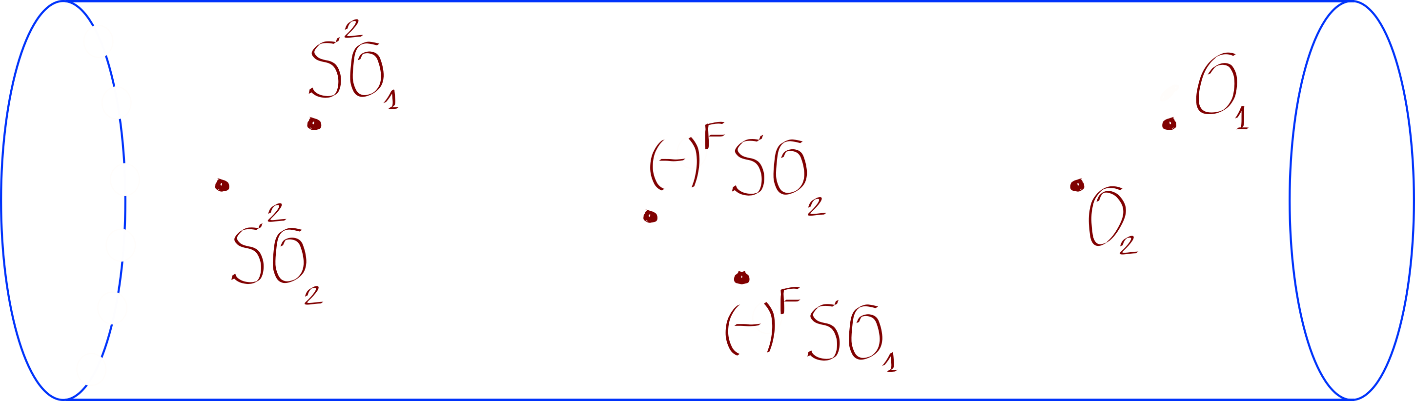
\delta S=\epsilon_{1}\sum_{n=-\infty}^{\infty}\left((-1)^{F}S\right)^{n}\int d^{4}x\rho_{1}(x){\cal O}_{1}+\epsilon_{2}\sum_{n=-\infty}^{\infty}\left((-1)^{F}S\right)^{n}\int d^{4}x\rho_{2}(x){\cal O}_{2}

(219)

where $\epsilon_{1}$ and $\epsilon_{2}$ are two nilpotent coefficients. This is, essentially, an infinite periodic array (designed to satisfy Eq. (157)) of compactly supported deformations.

At the linearized level, i.e. assuming $\epsilon_{1}\epsilon_{2}=0$ , the two terms in the deformation transform in two infinite-dimensional representations, ${\cal H}_{1}$ and ${\cal H}_{2}$ . But if we do not assume $\epsilon_{1}\epsilon_{2}=0$ , then there will be a term in the SUGRA solution proportional to $\epsilon_{1}\epsilon_{2}$ , and it will not transform in ${\cal H}_{1}\otimes{\cal H}_{2}$ . We can consider the space of all possible completions of linearized solutions to nonlinear solutions. The terms proportional to $\epsilon_{1}\epsilon_{2}$ form a linear space $X$ , which, as a representation of $\bf g$ , is an extension:

0\longrightarrow\left[\begin{array}[]{c}\mbox{\tt\small solutions of}\cr\mbox{\tt\small linearized equations}\end{array}\right]\longrightarrow X\longrightarrow{\cal H}_{1}\otimes{\cal H}_{2}\longrightarrow 0

(220)

Even if we restrict on ${\bf g}_{\rm even}$ , there are such nontrivial extensions. The corresponding cocycle:

\psi\in H^{1}\left({\bf g}_{\rm even}\;,\;\mbox{Hom}\left({\cal H}_{1}\otimes{\cal H}_{2}\;,\;\left[\begin{array}[]{c}\mbox{\tt\small solutions of}\cr\mbox{\tt\small linearized }\cr\mbox{equations}\end{array}\right]\right)\right)

(221)

is nontrivial, the average of $\psi(\partial/\partial t)$ over the period (see Eq. (29)) is nonzero.

Let us insert, instead of an infinite array, just two operators: ${\cal O}_{1}$ and ${\cal O}_{2}$ . Consider the “retarded” solution excited by them. The waves will keep bouncing from the boundary of AdS, interacting in the middle. Therefore the $\epsilon_{1}\epsilon_{2}$ part will grow in global time like square of $t$ . We consider this a complication. To simplify the analysis, let us make four insertions (instead of just two):

\epsilon_{1}{\cal O}_{1}\;,\quad\epsilon_{2}{\cal O}_{2}\;,\quad\epsilon_{1}(-1)^{F}S{\cal O}_{1}\;,\quad\epsilon_{2}(-1)^{F}S{\cal O}_{2}

(222)

Then the terms linear in $\epsilon_{1}$ , as well as the terms linear in $\epsilon_{2}$ , will cancel in the future. But, before they cancel, there will be some interaction, generating terms proportional to $\epsilon_{1}\epsilon_{2}$ . In the future, the $\epsilon_{1}\epsilon_{2}$ -terms become a solution of the free equation. This is the “retarted” solution generated by these insertions, i.e. the one which is pure $AdS_{5}\times S^{5}$ in the past.

6.2 Monodromy vs boundary S-matrix

Let us suppose that $\rho_{1}$ is a delta-function at the point $b_{1}$ on the boundary, and $\rho_{2}$ delta-function at the point $b_{2}$ . Genarally speaking, every point $b$ on the boundary of AdS defines a Poincare patch, which can be defined as follows. Consider the future of $b$ , denote it ${\cal F}(b)$ (a subset of AdS). Notice that for any $n>0$ : $S^{n}{\cal F}(b)\subset{\cal F}(b)$ . Consider the “first fundamental domain” of ${\cal F}(b)$ with respect to the action of $S$ , i.e. the set of points $x\in{\cal F}(b)$ such $S^{-1}x\notin{\cal F}(b)$ . This is the Poincare patch ${\cal P}(b)$ corresponding to $b$ (the beige area on Figure 2). For the retarded solution corresponding to the insertions (222) all the interaction happens inside ${\cal P}(b_{1})\cap{\cal P}(b_{2})$ .

This implies that the average of $\psi(\partial/\partial t)$ , in the sense of Eq. (29) can be computed as the integral over ${\cal P}(b_{1})\cap{\cal P}(b_{2})$ . In fact, since the boundary-to-bulk propagator has support on the light cone, see Eq. (158), the integral is supported on $\partial{\cal P}(b_{1})\cap\partial{\cal P}(b_{2})$ . The integrand is the retarded propagator times triple-interaction vertex.

On the other hand, in the definition of the boundary S-matrix [29] the integration of the interaction vertex is over the whole Euclidean AdS. It is not clear to us how these two definitions are related.

6.3 Normalizable and non-normalizable contributions to monodromy

Notice that $\partial{\cal P}(b_{1})\cap\partial{\cal P}(b_{2})$ goes all the way to the boundary, therefore there is no reason why the monodromy would be a normalizable solution. However, the non-normalizable part is due to waves bouncing back and forth in AdS reflecting from the boundary. Therefore all the non-normalizable terms can be damped by making adjustments, of the order $\epsilon_{1}\epsilon_{2}$ , of the boundary conditions. In other words, correcting the defining Eq. (222) by adding some operators of the order $\epsilon_{1}\epsilon_{2}$ . Then, the monodromy of the modified array will be a normalizable solution. We used this in Section 5.5.

7 Discussion and open questions

A general theme of AdS/CFT is comparison of field theory computations with supergravity computations. The analysis of the present paper is incomplete, and potentially leaves a mismatch between field theory and supergravity. Indeed, on the field theory side we use the formalism of Sections 1.1, 1.2, 1.4. While on the supergravity side, we use the formalism of Sections 4.3, 4.4, which is similar but different.

7.1 Is it true that symmetries of QFT naturally act on the space of its deformations?

It is essential for our reasoning, that there is a natural action of the symmetries of QFT on the space of its deformations, Section 1.2. This action should be natural, i.e. should not depend on how we describe deformations. Strictly speaking, our reasoning in Section 1.2 used a particular way of thinking about the deformations. Therefore, we are in danger of using an unnatural definition.

7.2 Gauge group is not an invariant

Renormgroup invariants in QFT match certain cohomological invariants of the action of the group of gauge transformations of supergravity, as described in Section 4.4. But gauge group is not actually an invariant of the theory ¹³¹³ 13 Gauge transformations characterize the redundancy of the given Lagrangian desciption of the theory. A different Lagrangian descriptions of the same theory can have slightly different gauge symmetries.. Therefore, we are in danger of being non-invariant. However, the invariants which we describe in Section 4.4 actually depend, in some sense, on the cohomology of the gauge transformations. Our construction uses certain “flabbyness” of the algebra of gauge transformations, essentially allowing to reduce the cohomologies to those of $\bf g$ (using the Shapiro’s lemma). We hope that the cohomologies are invariant.

7.3 Maybe there is no mismatch

If our conjectures in Section 4.4 hold, namely:

•

Exists $M_{gauge-fixed}$ and
•

Solution of MC Equation does not depend on the choice of $M_{gauge-fixed}$

then the invariants of Section 4.4 just match the invariants on the QFT side, so there is no discrepancy. We think that this is, most likely, what actually happens.

7.4 Computation of the MC invariants

As we already mentioned in Section 5.10, an important open question is to develop the homological perturbation theory of [13, 14] and to actually compute the Maurer-Cartan invariants which we defined.

Acknowledgments

We want to thank Alexei Rosly for many useful discussions. This work was supported in part by FAPESP grant 2014/18634-9 “Dualidade Gravitac $\!\!,\tilde{\rm a}$ o/Teoria de Gauge”. and in part by RFBR grant RFBR 18-01-00460 “String theory and integrable systems”.

Appendix A AdS notations

A.1 Embedding formalism

We here consider massless Laplace equation in $AdS_{D}$ . We realize $AdS_{D}$ as a hyperboloid in ${\bf R}^{2,D-1}$ parametrized by coordinates $Z,\overline{Z},X^{1},\ldots,X^{D-1}$ . The equation of the hyperboloid is:

|Z|^{2}-\vec{X}^{2}=R^{2}

(223)

		$\displaystyle 2{\partial\over\partial Z}{\partial\over\partial\overline{Z}}-{\partial\over\partial\vec{X}}{\partial\over\partial\vec{X}}\;=\;{1\over R^{D}}{\partial\over\partial R}R^{D}{\partial\over\partial R}+{1\over R^{2}}{\bf L}\;=$		(224)
	$\displaystyle\;=\;$	$\displaystyle{1\over R^{2}}\left((\Delta+D-1)\Delta+{\bf L}\right)$		(225)

where $\Delta=R{\partial\over\partial R}$ and ${\bf L}$ is the Laplace operator on $AdS_{D}$ . Therefore, on harmonic functions:

{\bf L}=-\Delta(\Delta+D-1)

(226)

Our space-time is not just $AdS_{D}$ , but $AdS_{D}\times S^{D}$ . The formulas for Laplace operator on the sphere are completely analogous. To distinguish between AdS and sphere, we use indices $\rm A$ and $\rm S$ : ${\bf L}_{\rm A}$ , $\Delta_{\rm A}$ , ${\bf L}_{\rm S}$ , $\Delta_{\rm S}$ . The total Laplace operator on $AdS_{5}\times S^{5}$ is:

\square={\bf L}_{A}-{\bf L}_{S}

(227)

Therefore, for the scalar function to be harmonic in $AdS_{D}\times S^{D}$ :

\Delta_{\rm A}(\Delta_{\rm A}+D-1)\;=\;\Delta_{\rm S}(\Delta_{\rm S}+D-1)

(228)

This means:

\mbox{\tt\small either }\Delta_{\rm A}=\Delta_{\rm S}\quad\mbox{\tt\small or }\Delta_{\rm A}=-\Delta_{\rm S}-(D-1)

(229)

A.2 Solutions of wave equations

Consider the following family of scalar field profiles, parameterized by a real parameter $\alpha$ :

\phi_{\alpha}={f(\vec{X})+\sum_{n=1}^{[\mbox{deg}f\,/2]}(Z\overline{Z})^{n}f_{n,\alpha}(\vec{X})\over Z^{{\rm deg}f+\alpha}}

(230)

where $f_{n,\alpha}$ can be determined recursively from:

	$\displaystyle f_{n,\alpha}(\vec{X})\;=\;$	$\displaystyle-{n({\rm deg}f_{(n-1),\alpha}+\alpha-n)\over 2}{\partial\over\partial\vec{X}}{\partial\over\partial\vec{X}}f_{(n-1),\alpha}(\vec{X})$		(231)
	$\displaystyle f_{0,\alpha}(\vec{X})\;=\;$	$\displaystyle f(\vec{X})$		(232)

This solves the wave equation in ${\bf R}^{2,D-1}$

\left(2{\partial\over\partial Z}{\partial\over\partial\overline{Z}}-{\partial\over\partial\vec{X}}{\partial\over\partial\vec{X}}\right)\phi_{\alpha}=0

(233)

Therefore:

{\bf L}_{\rm A}\phi_{\alpha}=\alpha(D-1-\alpha)\phi_{\alpha}

(234)

Massless scalar in $AdS_{D}$

To solve the wave equation on $AdS_{D}$ , we take $\alpha=0$ :

{\bf L}_{\rm A}\phi_{0}=0

(235)

Massless scalar in $AdS_{D}\times S^{D}$

Let us parametrize $S^{D}$ by a unit vector ${\bf N}\in{\bf R}^{D+1}$ . Suppose that the $S^{D}$ dependence is a harmonic polynomial $Y({\bf N})$ of order $\Delta_{\rm S}$ . We must either take $\alpha=-\Delta_{S}$ or $\alpha=\Delta_{S}+D-1$ . The solution is:

\phi_{\alpha}(Z,\overline{Z},\vec{X})Y({\bf N})

(236)

Inhomogeneous equations, appearence of log terms

Consider the equation with nonzero right hand side: ${\bf L}_{\rm A}\phi=f$ . When $f$ is proportional to $\phi$ , the logarithmic terms appear. Indeed:

{\bf L}_{\rm A}\left.{\partial\over\partial\alpha}\right|_{\alpha=0}\phi_{\alpha}=-(D-1)\phi_{0}

(237)

and therefore:

{\bf L}^{-1}\phi_{0}=-{1\over D-1}\left.{\partial\over\partial\alpha}\right|_{\alpha=0}\phi_{\alpha}

(238)

This expression contains $\log Z$ . A somewhat special case is the equation:

{\bf L}_{\rm A}\phi_{1}=1

(239)

The solution is:

\phi_{1}={1\over 2(D-1)}\left.{\partial\over\partial\alpha}\right|_{\alpha=0}\left({1\over Z^{\alpha}}+{1\over\overline{Z}^{\alpha}}\right)={1\over 2(D-1)}\log(Z\overline{Z})

(240)

One can think of $\phi_{\alpha}$ as a family, parametrized by $\alpha$ , of field profiles, taking values in a different representation for each $\alpha$ . (All these representations are subspaces of one large space.) The value of the Casimir operator ${\bf L}_{\rm A}$ is given by Eq. (234). When $\alpha=0$ it is zero. From this point of view, Eq. (238) is a particular case of the following general construction. Suppose that we have an operator $\bf L$ acting on a representation space $V$ of $\bf g$ , commuting with $\bf g$ , and $V$ is a continuous direct sum of subrepresentations $V_{\alpha}$ parametrized by a parameter $\alpha$ , such that the restriction of ${\bf L}$ on each $V_{\alpha}$ is the multiplication by $\alpha$ . For $v_{0}\in V_{0}$ , we want to find $w$ such that $Lw=v_{0}$ . Consider a 1-parameter family of vectors $v(\alpha)\in V_{\alpha}$ such that $v(0)=v_{0}$ . Then $w=\left.{d\over d\alpha}\right|_{\alpha=0}v(\alpha)$ . We only need a 1-jet of the family. If it is possible to find a map:

V_{0}\rightarrow\mbox{\tt\small the space of 1-jets of paths in }V\mbox{ \tt\small passing through }V_{0}

(241)

commuting with with the symmetry, then the equation $Lw=v_{0}$ can be solved in a covariant way:

w=\left.{d\over d\alpha}\right|_{\alpha=0}v(\alpha)

(242)

For example, if $V$ were equipped with a metric, we could pick for each $v_{0}$ the path going through $v_{0}$ with the velocity perpendicular to $V_{0}$ . But in our context, there is no invariant metric, and there is no ${\bf g}$ -covariant invertion of ${\bf L}$ .

We can construct a sequence of $t$ -independent functions:

$\displaystyle\phi_{0}\;=\;$	$\displaystyle 1$	(243)
$\displaystyle\phi_{1}\;=\;$	$\displaystyle\log(Z\overline{Z})$	(244)
$\displaystyle{\bf L}_{\rm A}\phi_{n}\;=\;$	$\displaystyle\phi_{n-1}$	(245)

They all depend only on $Z\overline{Z}$ and grow near the boundary of AdS as powers of $\log(Z\overline{Z})$ .

A.3 Functions participating in the perturbative expansion of nonlinear beta-deformation

We expect that nonlinear beta-deformation (and other finite-dimensional deformations) is expressed in terms of functions $\phi_{n}$ of Eq. (245) and their derivatives w.r.to $Z$ and $\bar{Z}$ , multiplied by polynomials of $\vec{X}$ and rational functions of $Z,\overline{Z}$ .

References

[1] M. Bianchi, D. Z. Freedman, and K. Skenderis, Holographic renormalization, Nucl. Phys. B631 (2002) 159–194 doi: 10.1016/S0550-3213(02)00179-7 [arXiv/hep-th/0112119].
[2] K. Skenderis, Lecture notes on holographic renormalization, Class. Quant. Grav. 19 (2002) 5849–5876 doi: 10.1088/0264-9381/19/22/306 [arXiv/hep-th/0209067].
[3] O. Aharony, B. Kol, and S. Yankielowicz, On exactly marginal deformations of N = 4 SYM and type IIB supergravity on AdS(5) x S**5, JHEP 06 (2002) 039 [arXiv/hep-th/0205090].
[4] M. A. Vasiliev, Higher spin gauge theories in various dimensions, Fortsch. Phys. 52 (2004) 702–717 doi: 10.1002/prop.200410167, 10.22323/1.011.0003 [arXiv/hep-th/0401177]. [,137(2004)].
[5] A. A. Sharapov and E. D. Skvortsov, Formal higher-spin theories and Kontsevich–Shoikhet–Tsygan formality, Nucl. Phys. B921 (2017) 538–584 doi: 10.1016/j.nuclphysb.2017.06.005 [arXiv/1702.08218].
[6] V. Arnold, Mathematical Methods of Classical Mechanics. Springer, 1997.
[7] R. G. Leigh and M. J. Strassler, Exactly marginal operators and duality in four-dimensional N=1 supersymmetric gauge theory, Nucl. Phys. B447 (1995) 95–136 doi: 10.1016/0550-3213(95)00261-P [arXiv/hep-th/9503121].
[8] A. W. Knapp, Lie Groups, Lie Algebras, and Cohomology. Princeton University Press, 1988.
[9] W. Schulgin and J. Troost, The Algebra of Diffeomorphisms from the World Sheet, JHEP 09 (2014) 146 doi: 10.1007/JHEP09(2014)146 [arXiv/1407.1385].
[10] N. Berkovits and P. S. Howe, Ten-dimensional supergravity constraints from the pure spinor formalism for the superstring, Nucl. Phys. B635 (2002) 75–105 [hep-th/0112160].
[11] A. Mikhailov, Symmetries of massless vertex operators in AdS(5) x S**5, Adv.Theor.Math.Phys. 15 (2011) 1319–1372 doi: 10.4310/ATMP.2011.v15.n5.a3.
[12] S. P. Milian, Supermultiplet of $\beta-$ deformations from twistors, arXiv/1607.06506 .
[13] O. A. Bedoya, L. Bevilaqua, A. Mikhailov, and V. O. Rivelles, Notes on beta-deformations of the pure spinor superstring in AdS(5) x S(5), Nucl.Phys. B848 (2011) 155–215 doi: 10.1016/j.nuclphysb.2011.02.012 [arXiv/1005.0049].
[14] H. A. Benítez and V. O. Rivelles, Yang-Baxter deformations of the $AdS_{5}\times S^{5}$ pure spinor superstring, JHEP 02 (2019) 056 doi: 10.1007/JHEP02(2019)056 [arXiv/1807.10432].
[15] A. Fayyazuddin and S. Mukhopadhyay, Marginal perturbations of N=4 Yang-Mills as deformations of AdS(5) x S**5, arXiv/hep-th/0204056 .
[16] O. Lunin and J. M. Maldacena, Deforming field theories with U(1) x U(1) global symmetry and their gravity duals, JHEP 05 (2005) 033 [arXiv/hep-th/0502086].
[17] H.-Y. Chen and K. Okamura, The Anatomy of gauge/string duality in Lunin-Maldacena background, JHEP 02 (2006) 054 doi: 10.1088/1126-6708/2006/02/054 [arXiv/hep-th/0601109].
[18] H. Flores and A. Mikhailov, On worldsheet curvature coupling in pure spinor sigma-model, arXiv/1901.10586 .
[19] B. L. Feigin and D. B. Fuchs, Cohomology of Lie groups and algebras (in Russian). VINITI t. 21, 1988.
[20] A. Mikhailov, Cornering the unphysical vertex, JHEP 082 (2012) doi: 10.1007/JHEP11(2012)082 [arXiv/1203.0677].
[21] D. Berenstein and S. A. Cherkis, Deformations of N=4 SYM and integrable spin chain models, Nucl. Phys. B702 (2004) 49–85 doi: 10.1016/j.nuclphysb.2004.09.005 [arXiv/hep-th/0405215].
[22] D. Bundzik and T. Mansson, The General Leigh-Strassler deformation and integrability, JHEP 01 (2006) 116 doi: 10.1088/1126-6708/2006/01/116 [arXiv/hep-th/0512093].
[23] C. Klimcik, On integrability of the Yang-Baxter sigma-model, J. Math. Phys. 50 (2009) 043508 doi: 10.1063/1.3116242 [arXiv/0802.3518].
[24] F. Delduc, M. Magro, and B. Vicedo, An integrable deformation of the AdS5xS5 superstring action, Phys. Rev. Lett. 112 (2014), no. 5 051601 doi: 10.1103/PhysRevLett.112.051601 [arXiv/1309.5850].
[25] T. J. Hollowood, J. L. Miramontes, and D. M. Schmidtt, An Integrable Deformation of the $AdS_{5}\times S^{5}$ Superstring, J. Phys. A47 (2014), no. 49 495402 doi: 10.1088/1751-8113/47/49/495402 [arXiv/1409.1538].
[26] B. Hoare and A. A. Tseytlin, Type IIB supergravity solution for the T-dual of the $\eta$ -deformed AdS ${}_{5}\times$ S⁵ superstring, JHEP 10 (2015) 060 doi: 10.1007/JHEP10(2015)060 [arXiv/1508.01150].
[27] A. Mikhailov, Finite dimensional vertex, JHEP 1112 (2011) 5 doi: 10.1007/JHEP12(2011)005 [arXiv/1105.2231].
[28] A. Mikhailov and S. P. Milián, A geometrical point of view on linearized beta-deformations, Lett Math Phys (2019) doi: 10.1007/s11005-019-01165-z [arXiv/1703.00902].
[29] E. Witten, Anti-de Sitter space and holography, Adv. Theor. Math. Phys. 2 (1998) 253–291 [arXiv/hep-th/9802150].

1 Introduction

1.1 Renormalization of the deformations of the action

1.2 Symmetries of undeformed theory act on deformations

1.3 Holographic renormalization

1.4 Geometrical abstraction

Tangent vectors as equivalence classes of trajectories

The role of supergeometry and infinite-dimensional geometry

1.5 Summary of this paper

Cohomological framework for holographic renormalization

Finite-dimensional representations have nontrivial cohomology

Plan

2 Obstacles to linearization of symmetry

2.1 Action of a symmetry in local coordinates

2.2 Maurer-Cartan equation

2.3 Gauge transformations

2.4 Tangent space to the moduli space of solutions of MC equation

2.5 Monodromy transformation

Additional assumption

2.6 Symmetries

2.7 Closed subsectors

3 Relation to tree level Feynman diagrams

3.1 Perturbation theory as a map T​M→Ω​MTM\rightarrow\Omega M

Lemma 0:

Proof

Lemma 1:

Proof

3.2 Amputation of the last leg

3.3 Trivial example

3.4 Example: classical CFT on 𝐑×Sd−1{\bf R}\times S^{d-1}

3.4.1 Realization of 𝐑×Sd−1{\bf R}\times S^{d-1} as the base of the lightcone

3.4.2 Conformal symmetry

3.4.3 Amputator

3.4.4 Relation to renormgroup

3.5 Comments on the structure of Ψ\Psi

3.5.1 Ψ\Psi is simpler than perturbative classical solutions

3.5.2 The condition of 𝐠\bf g-covariance is complicated

3.5.3 Can Ψ\Psi be bootstrapped?

4 Supergravity in AdS space

4.1 Holographic renormgroup

- Renormgroup flow on the boundary

- Classical solutions of SUGRA in the bulk

4.2 Gauge transformations of supergravity

4.3 Geometrical abstraction

4.4 Normal form of the action of 𝐚\bf a

4.4.1 General vector field tangent to 𝒪\cal O

Big Maurer-Cartan equation

4.4.2 Reduction to 𝐠⊂𝐚{\bf g}\subset{\bf a}

Assuming that there are no obstacles of the type Eq. (116)

4.4.3 Is Ψ\Psi an invariant? Deformations of Mg​a​u​g​e−f​i​x​e​dM_{gauge-fixed}.

Geometrical picture

In coordinates

4.4.4 Conclusion

4.5 Pure spinor formalism

When n=1n=1

4.6 If Mg​a​u​g​e−f​i​x​e​dM_{gauge-fixed} does not exist

In the rest of this Section

4.7 Normalizable SUGRA solutions

4.8 Non-normalizable SUGRA solutions

4.9 Simplest non-periodic linearized solution

5 Beta-deformation and its generalizations

5.1 Description of beta-deformation in pure spinor formalism

5.2 Restriction of Ψ\Psi to even subalgebra

5.3 Infinite-dimensional extension of finite-dimensional ℋ\cal H

Log terms

Structure of ℋ^\widehat{\cal H}

Example of cocycle

5.4 Renormgroup flow generates infinite-dimensional representations

5.5 Nonlinear beta-deformations have trivial monodromy

5.6 Lifting of Ψ\Psi to superalgebra

Step 1: construct an element of H1​(𝐠,Hom​(𝐠,ℋ))H^{1}\left({\bf g},\mbox{Hom}({\bf g},{\cal H})\right)

Step 2: compose it with an intertwiner S2​ℋ→𝐠S^{2}{\cal H}\rightarrow{\bf g}

5.7 Construction of the intertwiner S2​ℋ→𝐠S^{2}{\cal H}\rightarrow{\bf g}

Algebraic preliminaries

Description of ℋ\cal H

Description of the intertwiner

Intertwiner maps H1​(𝐠,Hom​(𝐠,ℋ))H^{1}\left({\bf g},\mbox{Hom}({\bf g},{\cal H})\right) to H1​(𝐠,Hom​(S2​ℋ,ℋ))H^{1}\left({\bf g},\mbox{Hom}(S^{2}{\cal H},{\cal H})\right)

5.8 Structure of S2​ℋS^{2}{\cal H}

5.9 Role of ψ\psi in anomaly cancellation

5.10 Outline of computation

5.11 Other finite-dimensional deformations

3.1 Perturbation theory as a map $TM\rightarrow\Omega M$

3.4 Example: classical CFT on ${\bf R}\times S^{d-1}$

3.4.1 Realization of ${\bf R}\times S^{d-1}$ as the base of the lightcone

3.5 Comments on the structure of $\Psi$

3.5.1 $\Psi$ is simpler than perturbative classical solutions

3.5.2 The condition of $\bf g$ -covariance is complicated

3.5.3 Can $\Psi$ be bootstrapped?

4.4 Normal form of the action of $\bf a$

4.4.1 General vector field tangent to $\cal O$

4.4.2 Reduction to ${\bf g}\subset{\bf a}$

4.4.3 Is $\Psi$ an invariant? Deformations of $M_{gauge-fixed}$ .

When $n=1$

4.6 If $M_{gauge-fixed}$ does not exist

5.2 Restriction of $\Psi$ to even subalgebra

5.3 Infinite-dimensional extension of finite-dimensional $\cal H$

Structure of $\widehat{\cal H}$

5.6 Lifting of $\Psi$ to superalgebra

Step 1: construct an element of $H^{1}\left({\bf g},\mbox{Hom}({\bf g},{\cal H})\right)$

Step 2: compose it with an intertwiner $S^{2}{\cal H}\rightarrow{\bf g}$

5.7 Construction of the intertwiner $S^{2}{\cal H}\rightarrow{\bf g}$

Description of $\cal H$

Intertwiner maps $H^{1}\left({\bf g},\mbox{Hom}({\bf g},{\cal H})\right)$ to $H^{1}\left({\bf g},\mbox{Hom}(S^{2}{\cal H},{\cal H})\right)$

5.8 Structure of $S^{2}{\cal H}$

5.9 Role of $\psi$ in anomaly cancellation

Massless scalar in $AdS_{D}$

Massless scalar in $AdS_{D}\times S^{D}$