Automated Detection of Solar Radio Bursts using a Statistical Method
keywords
Corona, Radio Emission; Radio Bursts; Instrumentation and Data Management1 Introduction
Radio bursts from the Sun play an important role in understanding solar atmosphere, solar wind, and particularly coronal mass ejections. Many of these bursts provide clues to understand space weather. Radio bursts are observed over a wide range of frequencies (from few GHz to kHz), and they help to probe the solar atmosphere from chromospheric heights to 1 AU and beyond. Based on their morphology and frequency drift speeds (drift rates) in the dynamic spectrograms, they are classified into five primary types viz. Type I, Type II, Type III, Type IV and Type V bursts (Wild 1967). Type J and Type U are the other complex bursts which are often observed in the solar corona (Kundu 1965; McLean and Labrum 1985).
Technology advancements have enabled us to observe solar radio bursts with sophisticated telescopes both from ground and space. For example, some ground based solar dedicated radio spectrographs are: Radio Solar Telescope Network (RSTN) operated by US airforce (Guidice et al. 1981), Gauribidanur Low frequency Solar Spectrograph (GLOSS) in India (Kishore et al. 2014), Hiraiso Radio Spectrograph (HiRAS) in Japan (Kondo et al. 1994), IZMIRAN in Russia (Gorgutsa et al. 2001), ARTEMIS-IV in Greece (Caroubalos et al. 2001) and many others11 1 https://www.astro.gla.ac.uk/users/eduard/cesra/?page_id=187. Apart from these, there are more than 150 observing stations setup around the world to monitor the Sun, 24 hours a day. Presently about 52 of them regularly upload/provide data to a server at the University of Applied Sciences (FHNW) in Brugg/Windisch, Switzerland. The data processing is managed at Swiss Federal Institute of Technology (ETH) in Zurich, Switzerland. All these stations jointly constitute the e-CALLISTO network22 2 http://www.e-callisto.org/(Benz et al. 2009; Sasikumar Raja et al. 2018). Space based observations at MHz are carried out using WAVES-WIND (Bougeret et al. 1995), and WAVES-STEREO (Kaiser 2005; Rucker et al. 2005) instruments. There are attempts to combine these space-based observations with the ground-based observations also (see for example Hariharan et al. 2016). All these spectrometers produce large datasets. For instance, in the present work, we used data observed using the CALLISTO spectrometer located at Gauribidanur observatory, India (Monstein, Ramesh, and Kathiravan 2007) that recorded files in two years. Therefore, manual identification of the radio bursts is not possible - hence the present work.
In recent times, machine learning applications are widely used in classification problems. It is known that, if we want to apply them to classify various types of solar radio bursts, the machine needs to be ‘trained’ and we need large set of data for each type of burst. As mentioned previously, manual identification of bursts in a training dataset is an onerous task. We also know that more the training data, better the performance of classifier (classification method). Hence, in this paper, we present an algorithm to automatically identify the radio bursts using a statistical method. The developed algorithm could detect whether or not there is a radio burst present in the spectrogram. Our primary motivation is to use the database prepared using the algorithm described in the paper, and develop an automated classifier which would classify various types of individual bursts. So far, there have attempts to automatically identify specific type of bursts (Lobzin et al. 2009; Lobzin et al. 2010; Lobzin, Cairns, and Zaslavsky 2014; Salmane et al. 2018; Zhang, Wang, and Ye 2018). However, automatic recognition of all types of bursts was never reported in the literature to the best of our knowledge.
In this paper, \irefsec:obs describes the observational details of the data used. In \irefsec:method, a novel statistical method to automatically identify the radio bursts is explained. \irefsec:res describes the performance of the algorithm using the receiver operating characteristics and analysis of all type III bursts observed in the year 2014. The summary, conclusion and future scope are discussed in \irefsec:sum.
2 Observations
sec:obs
The observations of e-CALLISTO spectrometers began in the year 2009. Since then, so far stations are installed around the globe as previously mentioned. Most of the stations use the log-periodic dipole antenna (LPDA) as the primary receiving element (see for example Kishore et al. 2014; Sasikumar Raja et al. 2013a). The e-CALLISTO receiver is designed to operate over the bandwidth 45-870 MHz. But different e-CALLISTO stations operate over different user selected radio windows based on the local conditions. For this study, we used the data observed at Gauribidanur observatory, located at longitude E, latitude N and meters above sea level (Ebenezer et al. 2007; Ramesh 2011; Kishore et al. 2015). At Gauribidanur observatory, spectral radio observations of the Sun with the e-CALLISTO are carried out everyday during 02:30 - 11:30 UT. The frequency range of operation is 45-450 MHz. The observed data, about 400 frequencies per sweep, are stored as FITS-files. The time resolution of the instrument is 0.25 sec at the rate of 200 channels per spectrum (i.e. 800 pixels/sec). The integration time is 1 msec and the radiometric bandwidth is about 300 kHz. The overall dynamic range of the e-CALLISTO is dB.
Statistically, the number of radio bursts observed during the solar maximum are larger (in comparison to the solar minimum). Therefore, we selected the years 2013 and 2014 (solar maximum of solar cycle 24) for this study. The detailed method and results are discussed in the subsequent sections.
3 Method
sec:method


(a) (b)

(c) (d)
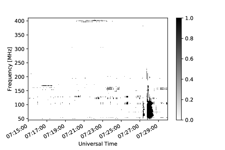
In order to classify the radio bursts, the basic observed parameters used from the dynamic spectrograms are area, slope, relative intensity, start and end time of the bursts, and the frequency range over which they were observed. We carefully inspected the above parameters to identify the radio bursts. The terrestrial radio frequency interference (RFI) appear as continuous features in dynamic spectra (for example FM, television, satellite signals, etc.); in some cases they appear as sharp pulses. By contrast, solar radio bursts drift as they propagate from high to low frequencies. We identify and eliminate the RFI making use of this key difference between RFI and radio bursts. The drift rate of the radio bursts can be measured using the Equation \irefeq:vd. This is one of the main parameters which we use to identify solar radio bursts from the data. Figure \ireffig:rb shows the spectrogram observed on 04 January 2013. Panel (a) shows the observed raw spectrogram (before processing). We calculate the median over time for every frequency channel and the resultant column matrix is subtracted from every column of the raw data corresponding to the spectrogram shown in panel (a). After median filtering (background subtraction) most of the continuous local RFI were eliminated (see panel (b)). We repeated this process for the entire dataset observed in the year 2013 (Set-P). We found the standard deviation (i.e. ) of the entire processed Set-P to be 0.6 dB. We selected the dB as the initial cut-off to identify whether or not there is a solar radio burst present in the frame. To reduce complexity, we converted every processed image to a binary image; i.e., if the signal is greater than 3 dB count we assigned the number one; else the number is zero. The binary image is shown in panel (c). Using the binary images, contours of the images were traced using the ‘opencv’ python library and measured the area () and coordinates of the contours. In the e-CALLISTO spectrometers, channels with high RFI are avoided due to practical reasons. Therefore, in the cases where the radio bursts intercept the RFI band, our algorithm underestimates the area. For instance, at Gauribidanur observatory, the FM band ( MHz) was not used and therefore, the measured was underestimated by a factor duration of the radio burst. However, this factor does not significantly impact our results.
By knowing the coordinates, we calculated the slope (, also called f-t range ratio) of the radio bursts using
| (1) |
where and are the maximum and minimum frequencies respectively, , are the start and end times of the radio burst. As previously described, most of the RFI appear as horizontal and vertical lines. They are successfully eliminated by selecting the in the range .
We find that and alone are not sufficient to automatically identify the bursts. The area depends on the bandwidth and duration of the observed burst. At the same time, we found that the drift rate can mislead the algorithm for smaller and . Therefore, we defined a new parameter called the Area Slope Index (ASI):
| (2) |
If the maximum ASI measured for each file is greater than a certain threshold, we conclude that there is at least one solar radio burst present in the image. If the ASI is less than threshold, we conclude that no significant solar radio burst is present in the image.


In order to decide the ASI threshold, we manually separated the bursts observed in the year 2013 and named it as Set-B. We measured the probability of finding the number of bursts for a given ASI value (), for Set-B using
| (3) |
where , are the number of bursts for a given ASI and the total number of bursts in Set-B respectively.
Similarly, using the complete dataset observed in 2013 (Set-U, that includes the data with bursts and without bursts), we defined another parameter,
| (4) |
where , are the number of bursts for given ASI and the total number of bursts in the Set-U respectively.
The ratio of equations \irefeq:pb and \irefeq:pu (which gives , the probability ratio) for different ASI is calculated using
| (5) |
The probability ratio is then plotted with respect to ASI as shown in Figure \ireffig:ratio. From Figure \ireffig:ratio, we find that corresponds to an . As mentioned in the flowchart (Figure \ireffig:fc), if the is greater than the cut-off value of , we conclude that the corresponding image has at least one solar radio burst. Otherwise, there is no burst present in the image. We used this method to identify all the solar radio bursts in the years 2013 and 2014. We note here that for certain ASI values, there might be no images with radio bursts present - hence the value is zero as seen in Figure \ireffig:ratio.
Radio emission from the ‘quiet’ Sun component remains relatively constant throughout the solar cycle. The slowly varying component varies with the solar cycle, but this is mostly observed at microwave frequencies. Due to sensitivity limitations neither the quiet Sun, nor the slowly varying components of radio emission can be observed using e-CALLISTO. The non-thermal radio bursts are easily observed with the e-CALLISTO, since they are comparatively stronger. Furthermore, although the occurrence rate of solar radio bursts varies with solar cycle, their characteristic properties (i.e. , bandwidth and duration of the radio burst) vary only minimally. Therefore the ASI cut-off (which depends on , bandwidth and duration of the radio burst) remains unchanged throughout the solar cycle. The performance of the classifier is discussed in the \irefsec:res.


4 Results and Discussions
sec:res
4.1 Performance of the algorithm
We processed the raw data and identified the radio bursts using the method described in the \irefsec:method and Figure \ireffig:fc. Using the receiver operating characteristics (ROC), we studied the performance of the classifier (Fawcett 2006). Herewith, we summarize the necessary terms for the sake of completeness. If the instance is positive and it is classified as positive then it is termed as ‘true positive’. If the instance is negative and is classified as positive, then it is called ‘false positive’. By manually counting these parameters in the classified dataset (by the algorithm), we measured the ‘true positive’ rate (tp rate or recall) using
| (6) |
where TP and P are the positives correctly classified and the total number of positive instances.
We also measured the ‘false positive’ rate (fp rate or false alarm rate) of the classifier using
| (7) |
where FP and N are negatives incorrectly classified and the total negative number of instances.
By knowing the tp rate and fp rate (see Equations \irefeq:tpr and \irefeq:fpr), we calculated the recall and precision using
| (8) |
| (9) |
Note that the high value of recall and precision indicate the small number of ‘false negatives’ (i.e., where the instance is positive and classified as negative) and ‘false positives’ respectively. The calculated values of recall and precision for different ASI cut-offs are tabulated in Table \ireftable-1. In the year 2013, for the significant ASI (i.e., ), the calculated recall and precision are and respectively. The recall and precission for the dataset observed in 2014 (Set-Q, for the same ASI value) are and respectively. The recall and precision for different ASI values are shown in Figure \ireffig:scales. It shows that the parameter recall is more or less consistent for both Set-P and Q. However, the precision shows a difference of between Set-P and Q. We found that the improved precision in the year 2014 is due to the reduced RFI and the availability of the dataset.
| S. | ASI | Set-P | Set-Q | ||
|---|---|---|---|---|---|
| No. | () | Recall | Precision | Recall | Precision |
| (1) | (2) | (3) | (4) | (5) | (6) |
| 1 | 1312 | 95.82 | 50.00 | 95.67 | 61.70 |
| 2 | 1394 | 93.59 | 51.85 | 93.75 | 63.40 |
| 3 | 1476 | 92.76 | 53.45 | 92.55 | 63.90 |
| 4 | 1558 | 92.20 | 55.26 | 90.87 | 66.08 |
| 5 | 1640 | 91.09 | 56.57 | 89.18 | 66.85 |
| 6 | 1722 | 91.09 | 56.97 | 87.74 | 67.72 |
| 7 | 1804 | 90.25 | 57.86 | 86.30 | 68.38 |
4.2 Preliminary analysis of Type III bursts
sec:typeIII We carried out a preliminary analysis of all the type III bursts detected during the year 2014 using the automatic detection method described in this paper. We found a total of 238 type III bursts during our observing period ( 02:30 - 11:30 UT). Out of the above, 88 type III bursts were associated with GOES soft X-ray and/or Halpha flares33 3 https://cdaw.gsfc.nasa.gov/CME˙list/NOAA/org˙events˙text/, 44 4 https://www.ngdc.noaa.gov/stp/space-weather/solar-data/solar-features/solar-flares/x-rays/goes/xrs/goes-xrs-report˙2014.txt, 55 5 http://www.lmsal.com/solarsoft/ssw/last˙events-2014/, 66 6 http://hec.helio-vo.eu/hec/hec˙gui.php. Note that we define a type III burst to be flare associated if it occurred during the onset-end phase of the flare. The observational details of the Type III bursts and associated flares are provided in Appendix (see Table \ireftab-2). The remaining 150 type III bursts were not associated with any flare. These 150 bursts were probably due to weak energy releases in the solar atmosphere reported earlier in the literature (for example, Ramesh et al. 2010; Ramesh et al. 2013; Saint-Hilaire, Vilmer, and Kerdraon 2013; Sasikumar Raja and Ramesh 2013b; Mugundhan, Hariharan, and Ramesh 2017; James, Subramanian, and Kontar 2017; James and Subramanian 2018; Sharma, Oberoi, and Arjunwadkar 2018).


We also find that of the type III bursts in our list were observed below 200 MHz (left panel of Figure \ireffig:type3). An inspection of the source region of the associated flares indicate a pattern. While the flare locations are uniformly distributed between and longitude for bursts with upper frequency cut-off MHz, they are limited to longitude for bursts with upper frequency cut-off MHz (see right panel of Figure 5). This seems to indicate that bursts with higher starting frequencies are more directive. A detailed investigation of these results (using more data) will be reported elsewhere.
5 Summary and Conclusions
sec:sum
In this paper, we have presented an automated method to detect solar radio bursts. Although this method doesn’t classify the types of radio bursts, it is able to discriminate between dynamic spectra with and without solar radio bursts. Our algorithm can operate with all standard image formats and does not need FITS files. The method is tested on two years of e-CALLISTO data observed at Gauribidanur observatory. Using this method, we have identified 1182 radio bursts during January 2013 - April 2018. The list of these bursts can be found at (http://www.iiserpune.ac.in/˜p.subramanian/Bursts.zip). Furthermore, we studied all type III bursts observed in the year 2014 and found that of the bursts observed were below 200 MHz. The source region of the associated flares were close to the disk center (i.e. heliographic longitude ) for bursts with upper frequency cut-off MHz (Figure \ireffig:type3).
We have defined an Area Slope Index (ASI) and found that the dynamic spectra images with ASI have at least one solar radio burst. Using this ASI threshold, the recall for this method is over 95% and the precision is between 50 and 61%. The precision and recall for different ASI values are shown in Figure \ireffig:scales. The precision of the method can be improved (at the cost of poor recall by increasing the ASI cut-off) and vice versa. The precision can also be improved by comparing with the observations at other e-CALLISTO stations. One of the drawbacks of this method is that the weak radio bursts whose SNR is are insensitive to this method. Better data (which can allow for a lower SNR cutoff) can overcome this drawback.
A successful classifier with good performance can play a crucial role in understanding properties of solar radio bursts like drift rates, spectral indices and emission mechanisms, which are in turn are very useful in solving long-standing solar physics problems associated with coronal heating, propagation of coronal mass ejections and others. For instance, it is known that some kinds of radio bursts (such as Type II and Type IV) correlate with the geomagnetic storms, auroras and other space weather effects.
Accordingly, we plan to develop an automated burst classifier (that can discriminate between different kinds of bursts) in the future. We know that more the number of training datasets, better the performance of the classifier. However, this is a challenge by way of data processing. Since the e-CALLISTO stores one frame every 15 min and since observations are carried out for hours per day, it produces files in 5 years. Therefore, a 52 station e-CALLISTO network produces million files in 5 years. Each file size is kB. The file sizes are expected to be much higher for digital back end instrumentation based on FPGAs and fast ADCs (see for example Kumari et al. 2017; Mugundhan et al. 2018). Hence the necessity of a sophisticated algorithm to classify solar radio radio bursts. We would remark here that, there are another type of short duration ( s) spike bursts (for e.g., Tarnstrom and Philip 1972) with a small area are difficult to identify using the reported algorithm. In the future, we would like to develop an algorithm which would identify such bursts by cross-comparing the dynamic spectrograms observed by different observatories (which would help in mitigating local RFI). Such an algorithm can not only identify spike bursts, but also improve the efficiency of the scheme reported in this paper.
Acknowledgment
DS acknowledges the INSPIRE-SHE program of Department of Science Technology, India.
KSR acknowledges the financial support from the Science Engineering Research Board (SERB),
Department of Science Technology, India
(PDF/2015/000393). KSR acknowledges the NVIDIA Corporation for supporting this project by
donating the Titan Xp GPU. The authors would like to thank the anonymous
referee for his/her comments that helped in improving the manuscript.
Details of flare associated solar radio Type III bursts mentioned in Section \irefsec:typeIII are listed in Table \ireftab-2.
| Type III bursts | Flares | ||||||||
|---|---|---|---|---|---|---|---|---|---|
| Start | Frequency | Time | Active | Location | |||||
| S. | Date | time | (MHz) | (UT) | Class | region | |||
| No. | (UT) | Start | Stop | Onset | End | ||||
| (1) | (2) | (3) | (4) | (5) | (6) | (7) | (8) | (9) | (10) |
| 1 | 20140101 | 7:25:14 | 47 | 143 | 07:21 | 07:29 | C | 11940 | S12W47 |
| 2 | 20140126 | 8:28:44 | 45 | 219 | 08:26 | 09:33 | C | 11967 | S14E85 |
| 3 | 20140126 | 10:07:31 | 45 | 171 | 10:05 | 10:19 | C | 11960 | S15W24 |
| 4 | 20140129 | 4:16:44 | 45 | 157 | 04:06 | 04:42 | C | 11967 | S12E65 |
| 5 | 20140129 | 6:54:50 | 45 | 161 | 06:53 | 07:34 | C | 11967 | S12E65 |
| 6 | 20140129 | 7:00:25 | 45 | 98 | 06:53 | 07:34 | C | 11967 | S12E65 |
| 7 | 20140129 | 7:28:47 | 45 | 168 | 06:53 | 07:34 | C | 11967 | S12E65 |
| 8 | 20140130 | 7:53:54 | 45 | 127 | 07:54 | 08:41 | M | 11967 | S12E52 |
| 9 | 20140131 | 5:32:56 | 45 | 168 | 04:46 | 05:17 | C | 11967 | S14E37 |
| 10 | 20140210 | 5:03:01 | 45 | 177 | 05:04 | 05:23 | C | 11974 | S12E30 |
| 11 | 20140215 | 8:24:09 | 45 | 148 | 08:25 | 08:39 | C | 11974 | S13W38 |
| 12 | 20140303 | 7:22:29 | 45 | 135 | 07:10 | 07:19 | C | 11989 | N07W31 |
| 13 | 20140415 | 7:06:00 | 45 | 315 | 07:04 | 07:11 | C | 12035 | S15E27 |
| 14 | 20140415 | 9:16:07 | 45 | 284 | 09:15 | 09:25 | C | 12035 | S14E25 |
| 15 | 20140416 | 3:20:38 | 45 | 106 | 03:03 | 03:16 | C | 12035 | S15E16 |
| 16 | 20140416 | 4:15:03 | 45 | 163 | 04:11 | 04:14 | C | 12042 | N19E79 |
| 17 | 20140416 | 5:01:50 | 45 | 181 | 04:57 | 05:14 | C | 12035 | S15E14 |
| 18 | 20140416 | 5:15:00 | 45 | 242 | 04:57 | 05:14 | C | 12035 | S15E14 |
| 19 | 20140416 | 5:34:13 | 45 | 111 | 05:21 | 05:38 | C | 12042 | N19E78 |
| 20 | 20140416 | 6:37:11 | 45 | 358 | 06:37 | 06:48 | C | 12035 | S17E13 |
| 21 | 20140416 | 6:44:04 | 45 | 312 | 06:37 | 06:48 | C | 12035 | S17E13 |
| 22 | 20140416 | 7:16:59 | 45 | 253 | 07:17 | 07:26 | C | 12034 | N03W01 |
| 23 | 20140416 | 8:19:42 | 45 | 152 | 08:12 | 08:20 | C | 12034 | N03W01 |
| 24 | 20140416 | 8:48:38 | 45 | 166 | 08:36 | 08:51 | C | 12035 | N19E75 |
| 25 | 20140419 | 9:18:44 | 45 | 105 | 09:17 | 09:22 | C | 2032 | N12W76 |
| 26 | 20140419 | 9:25:00 | 45 | 254 | 09:24 | 09:29 | C | 2036 | S15W42 |
| 27 | 20140501 | 4:06:00 | 45 | 180 | 03:58 | 04:04 | B | 12048 | N19W78 |
| 28 | 20140506 | 8:49:46 | 45 | 104 | 08:41 | 09:21 | M | 12051 | S15W84 |
| 29 | 20140604 | 7:20:52 | 45 | 105 | 07:07 | 07:16 | B | 12080 | S11E51 |
| 30 | 20140611 | 4:40:50 | 45 | 103 | 04:39 | 04:56 | C | 12087 | S12E71 |
| 31 | 20140611 | 5:31:15 | 45 | 152 | 05:30 | 05:36 | M | 12080 | S12W35 |
| 32 | 20140611 | 7:07:46 | 45 | 140 | 07:09 | 07:15 | C | 12080 | S12W36 |
| 33 | 20140611 | 8:58:06 | 45 | 104 | 08:59 | 09:10 | X | 12087 | S18E65 |
| 34 | 20140613 | 7:44:00 | 45 | 105 | 07:49 | 07:59 | M | 12089 | N18W01 |
| 35 | 20140613 | 7:50:30 | 45 | 108 | 07:49 | 07:59 | M | 12089 | N18W01 |
| 36 | 20140613 | 9:14:28 | 45 | 236 | 09:14 | 09:20 | C | 12087 | S17E41 |
| 37 | 20140613 | 9:16:20 | 45 | 180 | 09:14 | 09:20 | C | 12087 | S18E39 |
| 38 | 20140617 | 6:29:04 | 45 | 183 | 06:29 | 06:31 | B | 12087 | S20W07 |
| 39 | 20140617 | 7:38:40 | 45 | 154 | 07:36 | 07:46 | B | 12085 | S23W65 |
| 40 | 20140617 | 8:22:55 | 45 | 103 | 08:13 | 08:49 | C | 12093 | S11E61 |
| 41 | 20140617 | 10:07:01 | 45 | 169 | 09:59 | 10:05 | B | 12085 | S22W68 |
| 42 | 20140625 | 7:57:44 | 45 | 101 | 07:53 | 08:26 | B | 12096 | N09E42 |
| 43 | 20140628 | 7:35:57 | 45 | 173 | 07:36 | 07:49 | C | 12104 | S12E89 |
| 44 | 20140630 | 6:51:43 | 45 | 100 | 06:52 | 07:10 | C | 12100 | N09E20 |
| 45 | 20140630 | 7:04:16 | 45 | 104 | 06:52 | 07:10 | C | 12100 | N09E20 |
| 46 | 20140702 | 6:56:33 | 53 | 100 | 06:41 | 06:49 | C | 12106 | N15E45 |
| 47 | 20140702 | 7:39:07 | 53 | 153 | 07:34 | 07v38 | C | 12108 | S08E64 |
| 48 | 20140702 | 10:50:03 | 53 | 152 | 10:26 | 10:58 | C | 12102 | N15E28 |
| 49 | 20140708 | 2:31:09 | 54 | 98 | 02:31 | 02:36 | C | 12114 | S19E88 |
| 50 | 20140708 | 5:30:00 | 45 | 100 | 05:31 | 05:39 | C | 12113 | N09E60 |
| 51 | 20140709 | 4:37:42 | 51 | 176 | 04:37 | 04:39 | C | 12114 | S12E61 |
| 52 | 20140709 | 6:17:00 | 45 | 107 | 05:29 | 06:12 | C | 12113 | N11E48 |
| 53 | 20140723 | 7:28:02 | 45 | 228 | 07:28 | 07:51 | B | 12121 | N07E69 |
| 54 | 20140724 | 9:24:06 | 45 | 192 | 09:10 | 09:17 | B | 12121 | N08E56 |
| 55 | 20140725 | 6:58:50 | 45 | 280 | 06:57 | 07:07 | C | 12121 | N11E35 |
| 56 | 20140731 | 4:39:22 | 45 | 156 | 04:39 | 05:09 | B | 12127 | S05E30 |
| 57 | 20140810 | 6:41:42 | 45 | 138 | 06:44 | 06:52 | B | 12137 | S18W10 |
| 58 | 20140811 | 6:16:52 | 45 | 104 | 06:21 | 06:27 | B | 12137 | S17W24 |
| 59 | 20140811 | 10:07:26 | 45 | 208 | 10:09 | 10:12 | B | 12137 | S19W26 |
| 60 | 20140905 | 6:50:42 | 45 | 174 | 06:16 | 07:18 | C | 12152 | S13W45 |
| 61 | 20141003 | 3:04:36 | 45 | 179 | 02:57 | 03:15 | C | 12173 | S13W85 |
| 62 | 20141009 | 7:43:13 | 45 | 111 | 07:35 | 07:51 | C | 12182 | S18W46 |
| 63 | 20141011 | 4:12:09 | 45 | 104 | 03:26 | 04:25 | B | 12187 | S13E88 |
| 64 | 20141018 | 6:50:00 | 45 | 176 | 06:43 | 06:48 | C | 12192 | S13E72 |
| 65 | 20141021 | 4:05:18 | 45 | 177 | 04:03 | 04:07 | B | 12192 | S09E30 |
| 66 | 20141021 | 8:08:16 | 45 | 243 | 08:08 | 08:12 | C | 12192 | S09E31 |
| 67 | 20141024 | 3:55:45 | 45 | 107 | 03:56 | 04:02 | C | 12192 | S22W00 |
| 68 | 20141027 | 7:25:58 | 45 | 106 | 07:11 | 07:20 | C | 12192 | S18W48 |
| 69 | 20141031 | 9:21:06 | 45 | 280 | 09:19 | 09:27 | C | 12201 | S02E59 |
| 70 | 20141101 | 10:22:45 | 45 | 220 | 10:20 | 10:30 | C | 12201 | S05E47 |
| 71 | 20141102 | 3:06:28 | 45 | 184 | 03:05 | 03:11 | B | 12201 | S05E36 |
| 72 | 20141102 | 5:53:36 | 45 | 228 | 05:41 | 05:50 | B | 12201 | S05E34 |
| 73 | 20141103 | 3:47:59 | 45 | 360 | 03:47 | 03:56 | C | 12201 | S03E21 |
| 74 | 20141103 | 4:48:34 | 45 | 330 | 04:50 | 04:56 | C | 12201 | S03E18 |
| 75 | 20141103 | 7:04:00 | 45 | 253 | 07:06 | 07:09 | B | 12201 | S03E17 |
| 76 | 20141104 | 5:25:25 | 45 | 111 | 05:19 | 05:40 | C | 12205 | N16E84 |
| 77 | 20141108 | 4:54:31 | 45 | 108 | 05:02 | 05:10 | C | 12207 | S12E88 |
| 78 | 20141130 | 5:17:48 | 45 | 251 | 04:52 | 05:38 | C | 12222 | S18E31 |
| 79 | 20141130 | 8:42:58 | 45 | 404 | 07:58 | 09:15 | B | 12222 | S18E29 |
| 80 | 20141201 | 5:12:59 | 45 | 180 | 05:11 | 05:22 | C | 12217 | S16W25 |
| 81 | 20141203 | 2:33:05 | 45 | 186 | 02:30 | 02:37 | C | 12217 | S16W54 |
| 82 | 20141214 | 4:26:57 | 45 | 156 | 04:17 | 04:41 | C | 12241 | S11E74 |
| 83 | 20141214 | 4:30:29 | 45 | 107 | 04:17 | 04:41 | C | 12241 | S11E74 |
| 84 | 20141214 | 6:17:18 | 45 | 97 | 06:19 | 06:24 | C | 12227 | S02W79 |
| 85 | 20141214 | 6:21:12 | 45 | 166 | 06:19 | 06:24 | C | 12227 | S02W79 |
| 86 | 20141214 | 8:02:41 | 45 | 140 | 08:04 | 08:12 | C | 12237 | S20E51 |
| 87 | 20141214 | 8:25:05 | 45 | 187 | 08:25 | 08:37 | C | 12237 | S18E49 |
| 88 | 20141226 | 5:31:00 | 45 | 186 | 05:18 | 05:36 | C | 12249 | S12W37 |
References
- Benz et al. (2009) Benz, A.O., Monstein, C., Meyer, H., Manoharan, P.K., Ramesh, R., Altyntsev, A., Lara, A., Paez, J., Cho, K.-S.: 2009, A World-Wide Net of Solar Radio Spectrometers: e-CALLISTO. Earth Moon and Planets 104, 277. DOI. ADS.
- Bougeret et al. (1995) Bougeret, J.-L., Kaiser, M.L., Kellogg, P.J., Manning, R., Goetz, K., Monson, S.J., Monge, N., Friel, L., Meetre, C.A., Perche, C., Sitruk, L., Hoang, S.: 1995, Waves: The Radio and Plasma Wave Investigation on the Wind Spacecraft. Space Sci. Rev. 71, 231. DOI. ADS.
- Caroubalos et al. (2001) Caroubalos, C., Maroulis, D., Patavalis, N., Bougeret, J.-L., Dumas, G., Perche, C., Alissandrakis, C., Hillaris, A., Moussas, X., Preka-Papadema, P., Kontogeorgos, A., Tsitsipis, P., Kanelakis, G.: 2001, The New Multichannel Radiospectrograph ARTEMIS-IV/HECATE, of the University of Athens. Experimental Astronomy 11, 23. ADS.
- Ebenezer et al. (2007) Ebenezer, E., Subramanian, K.R., Ramesh, R., Sundararajan, M.S., Kathiravan, C.: 2007, Gauribidanur radio array solar spectrograph (GRASS). Bulletin of the Astronomical Society of India 35, 111. ADS.
- Fawcett (2006) Fawcett, T.: 2006, An introduction to roc analysis. Pattern Recognition Letters 27(8), 861 . ROC Analysis in Pattern Recognition. DOI. http://www.sciencedirect.com/science/article/pii/S016786550500303X.
- Gorgutsa et al. (2001) Gorgutsa, R.V., Gnezdilov, A.A., Markeev, A.K., Sobolev, D.E.: 2001, An upgrade of the izmiran’s solar digital radio spectrograph: First results. Astronomical and Astrophysical Transactions 20, 547. DOI. ADS.
- Guidice et al. (1981) Guidice, D.A., Cliver, E.W., Barron, W.R., Kahler, S.: 1981, The Air Force RSTN System. In: Bulletin of the American Astronomical Society, BAAS 13, 553. ADS.
- Hariharan et al. (2016) Hariharan, K., Ramesh, R., Kathiravan, C., Abhilash, H.N., Rajalingam, M.: 2016, High Dynamic Range Observations of Solar Coronal Transients at Low Radio Frequencies with a Spectro-correlator. ApJS 222, 21. DOI. ADS.
- James and Subramanian (2018) James, T., Subramanian, P.: 2018, Energetics of small electron acceleration episodes in the solar corona from radio noise storm observations. MNRAS 479, 1603. DOI. ADS.
- James, Subramanian, and Kontar (2017) James, T., Subramanian, P., Kontar, E.P.: 2017, Small electron acceleration episodes in the solar corona. MNRAS 471, 89. DOI. ADS.
- Kaiser (2005) Kaiser, M.L.: 2005, The STEREO mission: an overview. Advances in Space Research 36, 1483. DOI. ADS.
- Kishore et al. (2014) Kishore, P., Kathiravan, C., Ramesh, R., Rajalingam, M., Barve, I.V.: 2014, Gauribidanur Low-Frequency Solar Spectrograph. Sol. Phys. 289, 3995. DOI. ADS.
- Kishore et al. (2015) Kishore, P., Ramesh, R., Kathiravan, C., Rajalingam, M.: 2015, A Low-Frequency Radio Spectropolarimeter for Observations of the Solar Corona. Sol. Phys. 290, 2409. DOI. ADS.
- Kondo et al. (1994) Kondo, T., Isobe, T., Igi, S., Watari, S.-i., Tokumaru, M.: 1994, The New Solar Radio Observation System At Hiraiso. Communications Research Laboratory Review 40, 85. ADS.
- Kumari et al. (2017) Kumari, A., Ramesh, R., Kathiravan, C., Wang, T.J.: 2017, Strength of the Solar Coronal Magnetic Field - A Comparison of Independent Estimates Using Contemporaneous Radio and White-Light Observations. Sol. Phys. 292(11), 161. DOI. ADS.
- Kundu (1965) Kundu, M.R.: 1965, Solar radio astronomy. ADS.
- Lobzin, Cairns, and Zaslavsky (2014) Lobzin, V.V., Cairns, I.H., Zaslavsky, A.: 2014, Automatic recognition of type III solar radio bursts in STEREO/WAVES data for onboard real-time and archived data processing. Journal of Geophysical Research (Space Physics) 119, 742. DOI. ADS.
- Lobzin et al. (2009) Lobzin, V.V., Cairns, I.H., Robinson, P.A., Steward, G., Patterson, G.: 2009, Automatic recognition of type III solar radio bursts: Automated Radio Burst Identification System method and first observations. Space Weather 7, S04002. DOI. ADS.
- Lobzin et al. (2010) Lobzin, V.V., Cairns, I.H., Robinson, P.A., Steward, G., Patterson, G.: 2010, Automatic Recognition of Coronal Type II Radio Bursts: The Automated Radio Burst Identification System Method and First Observations. ApJ 710, L58. DOI. ADS.
- McLean and Labrum (1985) McLean, D.J., Labrum, N.R.: 1985, Solar radiophysics: Studies of emission from the sun at metre wavelengths. ADS.
- Monstein, Ramesh, and Kathiravan (2007) Monstein, C., Ramesh, R., Kathiravan, C.: 2007, Radio spectrum measurements at the Gauribidanur observatory. Bull. Astron. Soc. India 35, 473.
- Mugundhan, Hariharan, and Ramesh (2017) Mugundhan, V., Hariharan, K., Ramesh, R.: 2017, Solar Type IIIb Radio Bursts as Tracers for Electron Density Fluctuations in the Corona. Sol. Phys. 292, 155. DOI. ADS.
- Mugundhan et al. (2018) Mugundhan, V., Ramesh, R., Kathiravan, C., Gireesh, G.V.S., Hegde, A.: 2018, Spectropolarimetric Observations of Solar Noise Storms at Low Frequencies. Sol. Phys. 293(3), 41. DOI. ADS.
- Ramesh (2011) Ramesh, R.: 2011, Low frequency solar radio astronomy at the Indian Institute of Astrophysics (IIA). In: Astronomical Society of India Conference Series, Astronomical Society of India Conference Series 2. ADS.
- Ramesh et al. (2010) Ramesh, R., Kathiravan, C., Barve, I.V., Beeharry, G.K., Rajasekara, G.N.: 2010, Radio Observations of Weak Energy Releases in the Solar Corona. ApJ 719, L41. DOI. ADS.
- Ramesh et al. (2013) Ramesh, R., Sasikumar Raja, K., Kathiravan, C., Narayanan, A.S.: 2013, Low-frequency Radio Observations of Picoflare Category Energy Releases in the Solar Atmosphere. ApJ 762, 89. DOI. ADS.
- Rucker et al. (2005) Rucker, H.O., Macher, W., Fischer, G., Oswald, T., Bougeret, J.L., Kaiser, M.L., Goetz, K.: 2005, Analysis of spacecraft antenna systems: Implications for STEREO/WAVES. Advances in Space Research 36, 1530. DOI. ADS.
- Saint-Hilaire, Vilmer, and Kerdraon (2013) Saint-Hilaire, P., Vilmer, N., Kerdraon, A.: 2013, A Decade of Solar Type III Radio Bursts Observed by the Nançay Radioheliograph 1998-2008. ApJ 762, 60. DOI. ADS.
- Salmane et al. (2018) Salmane, H., Weber, R., Abed-Meraim, K., Klein, K.-L., Bonnin, X.: 2018, A method for the automated detection of solar radio bursts in dynamic spectra. Journal of Space Weather and Space Climate 8(27), A43. DOI. ADS.
- Sasikumar Raja and Ramesh (2013b) Sasikumar Raja, K., Ramesh, R.: 2013b, Low-frequency Observations of Transient Quasi-periodic Radio Emission from the Solar Atmosphere. ApJ 775, 38. DOI. ADS.
- Sasikumar Raja et al. (2013a) Sasikumar Raja, K., Kathiravan, C., Ramesh, R., Rajalingam, M., Barve, I.V.: 2013a, Design and Performance of a Low-frequency Cross-polarized Log-periodic Dipole Antenna. ApJS 207, 2. DOI. ADS.
- Sasikumar Raja et al. (2018) Sasikumar Raja, K., Subramanian, P., Ananthakrishnan, S., Monstein, C.: 2018, CALLISTO Spectrometer at IISER-Pune. ArXiv e-prints. ADS.
- Sharma, Oberoi, and Arjunwadkar (2018) Sharma, R., Oberoi, D., Arjunwadkar, M.: 2018, Quantifying Weak Nonthermal Solar Radio Emission at Low Radio Frequencies. ApJ 852, 69. DOI. ADS.
- Tarnstrom and Philip (1972) Tarnstrom, G.L., Philip, K.W.: 1972, Solar Radio Spike Bursts. A&A 16, 21. ADS.
- Wild (1967) Wild, J.P.: 1967, The Radioheliograph and the Radio Astronomy Programme of the Culgoora Observatory. Proceedings of the Astronomical Society of Australia 1, 38. DOI. ADS.
- Zhang, Wang, and Ye (2018) Zhang, P.J., Wang, C.B., Ye, L.: 2018, A type III radio burst automatic analysis system and statistic results for a half solar cycle with Nançay Decameter Array data. A&A 618, A165. DOI. ADS.