Uncertainty Estimates for Ordinal Embeddings
Abstract
To investigate objects without a describable notion of distance, one can gather ordinal information by asking triplet comparisons of the form “Is object closer to or is closer to ?” In order to learn from such data, the objects are typically embedded in a Euclidean space while satisfying as many triplet comparisons as possible. In this paper, we introduce empirical uncertainty estimates for standard embedding algorithms when few noisy triplets are available, using a bootstrap and a Bayesian approach. In particular, simulations show that these estimates are well calibrated and can serve to select embedding parameters or to quantify uncertainty in scientific applications.
1 Introduction
In a typical machine learning problem, we are given a data set of examples and a (dis)similarity function that quantifies the distance between the objects in . The inductive bias assumption of machine learning is then that similar objects should lead to a similar output. However, in poorly specified tasks such as clustering the biographies of celebrities, an obvious computable dissimilarity function does not exist. Nonetheless, humans often possess intuitive information about which objects should be dissimilar. While it might be difficult to access this information by quantitative questions (“On a scale from to , how similar are celebrities and ?”), it might be revealed using comparison-based questions of the type “Is object closer to or closer to ?” The answer to this distance comparison is called a triplet. The clear advantage of such an approach is that it removes the issues of a subjective scale across different participants. A common application for such ordinal data is crowd sourcing, where many untrained workers complete given tasks (Tamuz et al. 2011, Heikinheimo and Ukkonen 2013, Ukkonen et al. 2015). Ordinal information emerges for example as real data in search-engine query logs (Schultz and Joachims 2004). Given a list of search results, a document , on which a user clicked, is closer to a second clicked document than to a document , on which the user did not click.
The standard approach to deal with ordinal data in machine learning is to create Euclidean representations of all data points using ordinal embedding. In the classic literature, this approach is called non-metric multidimensional scaling (NMDS) (Borg and Groenen 2005) and has its origins in the analysis of psychometric data by Shepard 1962 and Kruskal 1964. In NMDS the objects are embedded into a low-dimensional Euclidean space while fulfilling as many triplet answers as possible. In recent years, such embedding methods have been extensively studied, and various optimization problems were proposed (Agarwal et al. 2007, Terada and von Luxburg 2014, Amid and Ukkonen 2015, Jain et al. 2016, Anderton et al. 2018), also including probabilistic models (Tamuz et al. 2011, van der Maaten and Weinberger 2012, Karaletsos et al. 2016).
Theoretical aspects of ordinal embeddings have been studied for the scenario where the original data comes from a Euclidean space of dimension . The consistency of ordinal embeddings in the large-sample limit as well as the consistency for the finite sample case up to a similarity transformation have been established (Kleindessner and von Luxburg 2014, Arias-Castro 2017). It is also known that actively chosen triplets are necessary to learn an embedding of points in (Jamieson and Nowak 2011, Jain et al. 2016) . As of now, there has been no theoretical analysis on the distortion of embeddings that are constructed from a set of much fewer than triplets. In this paper, we develop empirical methods that provide uncertainty estimates to characterize how certain a given embedding method is about its result when only few and possibly noisy training triplets are available.
We present two methods to obtain uncertainty estimates: one is based on a bootstrap approach, the other on a Bayesian approach. In both cases, we generate a distribution over embeddings which can then be used to compute the uncertainty about the answer of a triplet comparison or the point location. These uncertainty estimates improve upon ordinal embedding and address its limitations. In particular, we apply our uncertainty estimates to estimate the embedding dimension or to quantify uncertainty in psychophysics applications. In the experiments we examine whether the triplet uncertainty estimates are well calibrated. Lastly, we use the estimates to improve active selection of triplets. We find that our uncertainty estimates provide a valuable add-on to judge the quality of ordinal embeddings.
2 Setup and background on ordinal embedding
2.1 Setup
Let be a metric space and a finite data set. We consider a latent dissimilarity function on and abbreviate . In the following, we assume that no explicit dissimilarity values nor any other representations of the objects in are given to us. Instead, for three distinct points , and , we can observe the (possibly noisy) answer to the comparison: “Is or is ?” We call the answer to this question a triplet. Formally, a triplet is an ordered set of three points , encoding that the answer is “”. Similarly, denotes that the answer is “”. This answer can be noisy in the sense that it might be wrong compared to the ground truth dissimilarity. However, this ground truth is considered unknown and we only observe a set of noisy triplets, which we refer to as the training set.
A Euclidean embedding of the data set consists of points , written more compactly as . The parameter is called the embedding dimension. The function denotes the Euclidean distance function, abbreviated as . Let be the Euclidean distance matrix corresponding to the embedding .
Given a (noisy) triplet set , the goal of ordinal embedding is to find a representation of the data set in a low-dimensional space that recovers as many triplets as possible, that is we want to construct points such that
2.2 Ordinal embedding methods
The goal of this paper is to provide uncertainty estimates for ordinal embeddings and improve upon existing embedding methods. In the following, we briefly recall two popular embedding methods.
Crowd Kernel.
Tamuz et al. 2011 assume an explicit noise model by which the observed triplets have been generated. Given three points , the likelihood to obtain the triplet answer is given by
| (1) |
where is a parameter for regularization and numerical stability. A high value of indicates that a triplet is well modeled by the current embedding. Given a noisy set of triplets , the final embedding is obtained by minimizing the negative log-likelihood .
Stochastic Triplet Embedding (STE, van der Maaten and Weinberger 2012 ) suggests a more local variant where large violations receive nearly constant penalties and clearly satisfied triplets induce a nearly constant reward. Their Gaussian noise model leads to the triplet likelihood
| (2) |
In the same paper, the authors also suggest a more robust version of STE that replaces the Gaussian distribution by the more heavy-tailed -distribution, leading to what is called -STE (see supplement). The final embedding is constructed by minimizing the negative log-likelihood.
3 Computing uncertainty estimates of pairwise comparisons
Assume we are given a data set of abstract points, a noisy triplet set and an embedding algorithm. The goal is to generate a set of embedding samples and use the variance of such samples to capture uncertainty over point locations or triplet answers. We consider two approaches to generate embeddings in order to compute uncertainty estimates for ordinal embedding algorithms.
In a Bayesian approach, we use a prior distribution, either over embeddings or over distance matrices. As the second ingredient we use a likelihood function, encoding the probability of observing a certain triplet given an embedding or distances. Sampling from the corresponding posterior leads to a set of embeddings, or a set of distance matrices, respectively.
Our bootstrap approach proceeds like the following: we first subsample triplets (not points!) and secondly, we embed the points based on these triplets by the given embedding algorithm. Each repetition leads to a new embedding of the data points. As in the Bayesian approach, we can use this set of embeddings to evaluate uncertainties.
These uncertainty estimates capture uncertainties caused by the limited number of observed triplets and their possibly noisy nature. By construction, they cannot account for systematic model bias, which could be introduced by an inapt choice of embedding algorithm in the bootstrap, or a bad choice of likelihood in the Bayesian approach.
3.1 Bayesian approach for sampling embeddings
A Bayesian model is defined by a generative model that specifies prior and likelihood. We consider two variants. Our first attempt is to consider a prior over distance matrices. In order to calculate an uncertainty estimate for triplets, it is preferable to know directly the uncertainty of the two distances involved. However, this turns out to be challenging due to the specific properties of Euclidean distance matrices that would need to be modeled. Our second approach specifies a prior over embeddings. This turns out to be much more manageable despite the “detour” via embeddings to distances. In both cases, we use Gaussian distributions for the prior. Gaussians are a frequent choice of prior in the Bayesian literature. They are closely related to -norm regularizers in the statistical literature (Kanagawa et al. 2018) and amount to a similar set of assumptions and restrictions.
A prior over the distance matrix is supposed to incorporate as much prior knowledge about Euclidean distance matrices as possible, yet it should be easy to handle. Simple prior knowledge about Euclidean distance matrices is that they are symmetric, all entries are non-negative, diagonal entries are zero, and the entries fulfill the triangle inequality. These properties alone are not sufficient to characterize Euclidean distance matrices. We would need to incorporate even more complicated conditions (Dattorro 2005). However, it is hard to find a distribution of matrices that has its support exactly on Euclidean distance matrices. See the supplementary material for a first approach that employs a multivariate Gaussian prior over distance matrices to encode symmetry. It is non-trivial to encode more specific properties of distance matrices in an expressible prior. Because Bayesian models based on this simplistic but tractable prior did not behave satisfactorily in initial experiments we turn to a different approach.
A prior over embeddings is more manageable. We regard an embedding as a vector in . We assume the prior with . Furthermore, we assume that the embedded points are independently and identically distributed, that is is a block diagonal matrix. Overall, the Gaussian prior over embeddings is more restrictive than a prior over distance matrices since a distance matrix can originate from any point configuration. Yet, a prior over embeddings is a reasonable assumption because triplets put strong constraints on the embedding. Hence, the prior mainly provides a scale for the embeddings.
For a likelihood, we can use any function that appropriately describes how well a triplet is modeled, for example the STE likelihood (2) or other likelihood functions used by other embedding algorithms.
Combining either of the two priors with the chosen likelihood function yields two posterior distributions. When using the prior over embeddings we obtain
| (3) |
Both posterior distributions are not analytically tractable. However, it is possible to sample from them using a Markov Chain Monte Carlo algorithm or by applying variational methods. In this paper, we use the MCMC framework of elliptical slice sampling (ESS) by Murray et al. 2010. It is applicable for multivariate Gaussian priors and any likelihood function and can therefore be used for both posteriors. Elliptical slice sampling requires an initial sample . We use the fact that some embedding methods maximize a likelihood; for example we use STE to generate when sampling from a posterior that relies on the STE likelihood. As a result, the MCMC random walk begins at a maximum likelihood estimate and discovers the posterior distribution from there. Once we can sample from the posterior, we obtain distance matrices , either directly from , or via embeddings from .
3.2 Bootstrap approach for generating embeddings
In this section we propose a bootstrap approach to generate a set of embeddings. Given a training set of triplets and a sampling parameter , we uniformly draw many triplets out of without replacement to obtain a subset . After that, the given embedding method uses to embed the points into . Subsampling and embedding are repeated times, which results in embeddings. Note that we draw triplets without replacement for a single subset, but we do not divide into subsets. Therefore, we can choose arbitrarily high. The resulting embeddings can widely differ in scale and orientation. To make the embeddings comparable, we randomly select one of them as a reference embedding and use a Procrustes analysis to rotate and scale all the other embeddings to match the reference embedding as well as possible (Borg and Groenen 2005). This procedure results in embeddings , which give rise to distance matrices .
3.3 Computing uncertainty estimates
Given a set of distance matrices computed with either the Bayesian approach or the bootstrap, we can now compute uncertainties for all triplet answers. A naive approach is to compute the uncertainty of a triplet by evaluating in how many of the embeddings this triplet is true. However, this majority vote leads to bad results because it does not take the corresponding distances of a triplet into account. We propose the following model-based approach. From the set of distance matrices we first compute the entry-wise means and standard deviations :
We now assume that the distances are distributed as (an assumption that approximately holds in many applications). With these ingredients, a natural uncertainty estimate can be assigned to any triplet answer: the likelihood to observe the triplet answer is
| (4) |
where denotes the cdf of the standard normal distribution. If is close to , it signifies high uncertainty about . If is close to (or ), then the triplet is likely to be true (or the opposite is true).
Rather than computing the uncertainty of triplets, we can also evaluate uncertainties for each point position. Among embeddings we consider the mean and sample covariance of a single point:
where is the embedding of in the -th embedding . Note that these estimates make sense because in both our approaches, the embeddings are well-aligned and the distance matrices “comparable”: due to Procrustes analysis in the bootstrap approach, and due to the model-based approach in the Bayesian setting.
4 Using uncertainty estimates
In this section, we discuss four applications for our uncertainty estimates. First, we use our triplet uncertainty estimates to predict the true answers of triplet comparisons. Secondly, we estimate an appropriate embedding dimension for ordinal training data. Thirdly, we quantify the uncertainty of a psychophysics experiment by applying the point uncertainties. Finally, we query the most uncertain triplets in an active triplet selection setting.
4.1 Triplet prediction
Given a set of noisy triplets, the aim of triplet prediction is to predict the true answers both for unobserved triplet comparisons and noisy observed triplets. To use our uncertainty estimates for the triplet prediction problem, we introduce the possibility to abstain from a prediction. To this end, we introduce an “uncertainty threshold” . We predict if and if . If there is no prediction and we “abstain”. Note that by construction of the values we have that and thus, the above construction cannot lead to any inconsistencies.
The threshold can be used for a trade-off between the triplet prediction error and the abstention rate: when the threshold increases, we abstain more often, but the prediction error on the remaining predicted triplets decreases. It can also be observed that for a fixed threshold , the abstention rate decreases when we increase the number of training triplets because we are more and more certain about our predictions. See Section 5 for results.
4.2 Estimating the embedding dimension
When we employ an ordinal embedding approach and we are given real world ordinal information, it is often not clear how to choose the embedding dimension because the true dimension of the data is unknown. The naive approach is to use some measure to quantify the error of the embedding, and choose the dimension which leads to the best result. However, many such measures improve trivially with increasing dimension. This is analogous to overfitting – we achieve a low error for training triplets, but suffer a high error for unobserved triplets.
Instead, we now use uncertainty estimates to find a good embedding dimension. Given an embedding dimension we sample many embeddings as described above and compute the average uncertainty over all triplet answers. In regions of overfitting the uncertainty estimates reveal a higher variance due to many degrees of freedom, and in regions of underfitting the estimates reveal uncertainty due to contradicting triplets. As we can see in the experiments in Section 5.3, the average uncertainty is typically minimized for the correct dimension when using the bootstrap method. In other cases it can give an indication for a good embedding dimension depending on the intrinsic dimension of the data set. Additionally, the uncertainty estimates do not trivially decrease by increasing the embedding dimension.
4.3 Application in psychophysics
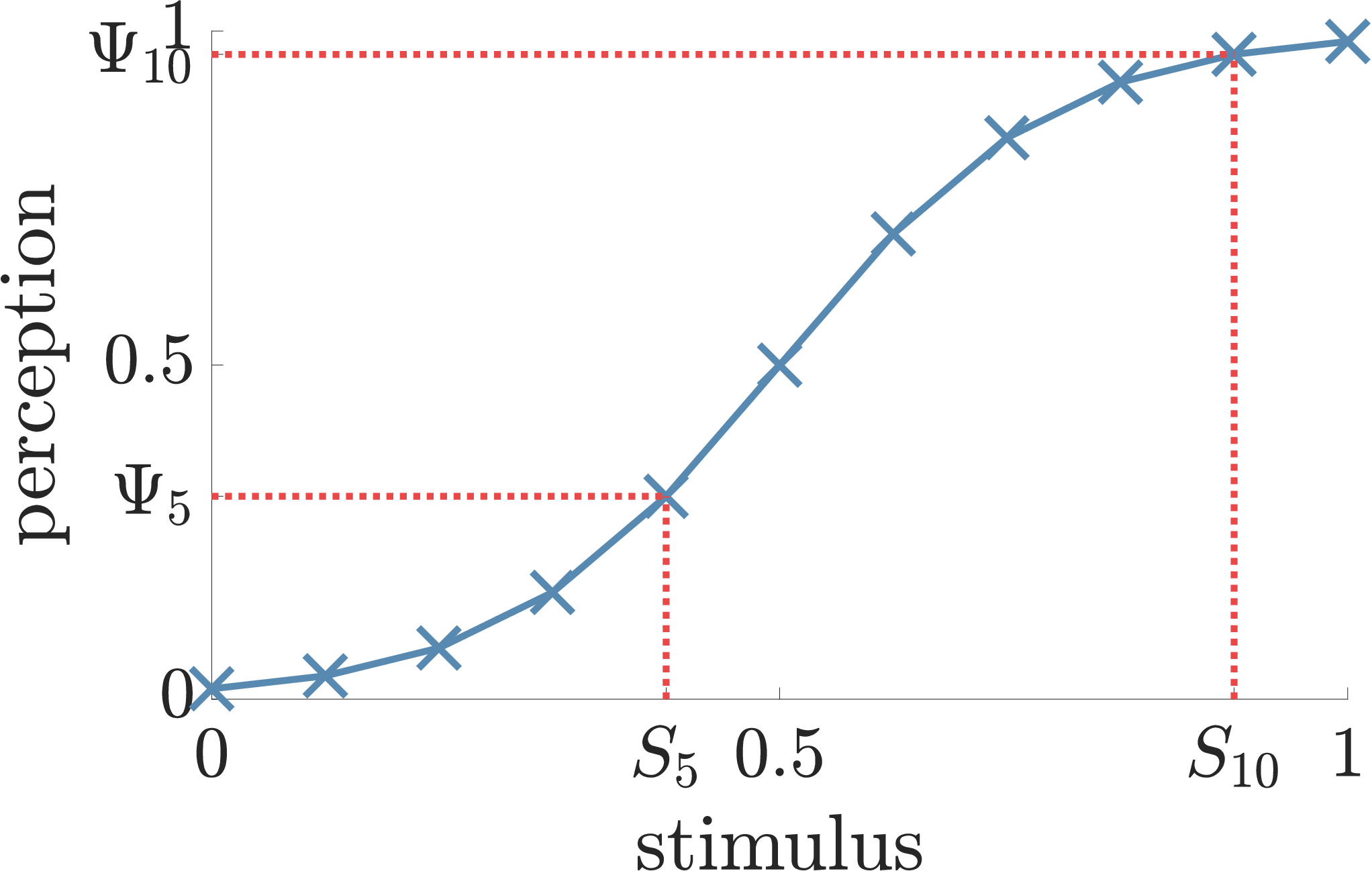
When ordinal embedding is used in a context of scientific data analysis, an analysis of uncertainties is often a crucial step. We want to illustrate this with an application in psychophysics. A standard task in this field is to estimate how physical stimuli are perceived by human observers. For example, the input might consist of images of increasing contrast, or of sounds of increasing frequency. The outcome of an experiment is supposed to show how this translates to the perceived increase of contrast, or sounds. See Figure 1 for an illustration where we plot a non-linear relation between an exemplary stimulus and its perception. While traditional methods such as the Steven’s Magnitude estimation (Gescheider 1997) try to quantitatively measure aspects of this relationship, a different approach is to use ordinal embeddings. Here, the idea is to ask participants to compare triplets of stimuli, and generate a one-dimensional embedding based on their triplet answers. This embedding corresponds to the projection of the curve in Figure 1 on the y-axis. We can now use our uncertainty estimates to additionally evaluate the uncertainties along the estimated perception curve.
To simulate a psychophysics experiment with a couple of human observers we assume that each observer perceives a stimulus following a fixed perception function (similar to Figure 1). The triplets that the human observer provides are created based on her corresponding perception function. Since every human observer perceives the stimuli differently, each observer has a different perception function and hence, gives different triplet answers. Finally, the set of all observed triplets contains contradictions depending on how different the perception functions of the observers are. In Section 4 we show that the uncertainties over point positions reveal how much the perception curves differ.
4.4 Active learning
For human observers providing triplets can be monotonous and boring after a while (Bijmolt and Wedel 1995), and crowd sourcing experiments are time consuming. Therefore, instead of asking all triplet comparisons, it can be advantageous to collect a small amount of the most informative triplets by an active approach. We propose our uncertainty estimates as a means to obtain a practical procedure for active triplet selection.
In this section we assume that there is a limited budget of triplets that can be collected. Before we query, the crowd provides a small set of random “seed triplets”. These triplets are answers to comparisons that have been drawn randomly with replacement from the set of all possible comparisons. Our estimates derived in (4) capture the uncertainty, which was introduced by the given seed set, for all triplets and determine which comparisons we should query next. The intuition is that the seed triplets determine the location of some points, while other points still have a lot of freedom. Therefore, we ask comparisons for which the answers are considered uncertain.
[.3]

[.3]

[.3]


Given a seed training set , we augment in the following way. First, we detect the triplets with highest uncertainty:
| (5) |
Triplets are binary answers, and our estimates assess the uncertainty about them: if is uncertain, then is uncertain to the same degree, since . Therefore, two complementary triplets will minimize (5). Then, we query the corresponding comparison from the crowd in order to observe the triplet answer, and add it to the training set . When collecting more triplets, we can query one by one, each time updating the uncertainty estimates, or we query bigger batches. Also note that a comparison might be queried several times.
In Section 5, we perform classification, clustering, and triplet prediction using actively queried triplet comparisons. Unfortunately, the results are disappointing: triplet prediction improves only by a small amount, which does not translate to an improvement for classification and clustering. This finding is in accord with our own experience in many simulations with a large variety of triplet selection mechanisms (landmark settings, geometry-based sampling): often, none of the intricate triplet sampling schemes significantly beat the naive strategy of random selection (Jamieson et al. 2015). However, it is in fact good news for practitioners. The advice based on the experiments in our paper is to simply query as many random comparisons as possible.
Related work on active triplet selection.
Some active approaches have already been reported in the literature on ordinal embeddings, however they are not practical for various reasons. Jamieson and Nowak 2011 consider an active triplet selection mechanism that is motivated from a theoretical point of view. It relies on a subroutine that outputs a consistent embedding if one exists (that is, an embedding that satisfies all true triplet answers). However, in a setting of noisy triplets, no algorithm can solve this problem.
Tamuz et al. 2011 propose an adaptive selection algorithm, which is similar to our Bayesian perspective. In order to collect a triplet for any point , they consider the posterior distribution over the location of in , involving all those triplets that have as the anchor. Then a pair of points is selected by a procedure that maximizes an information gain criterion, and the corresponding comparison is queried. Unfortunately, no code for this method is made available, but a data-driven approximation of the information gain can be used from Jamieson et al. 2015. However, it was not possible to produce competitive results within our framework. For the sake of completeness see the supplementary material for results comparing to the information gain criterion.


5 Experiments
In this section, we first examine the behavior of our uncertainty estimates when the number of training triplets or the noise level changes. Secondly, we consider the task of triplet prediction. Thirdly, we use our estimates to find an appropriate embedding dimension. Additionally, we simulate a psychophysics experiment and estimate point uncertainties. Lastly, we employ our estimates for an active learning approach and examine the performance with respect to triplet prediction, classification and clustering.
Method setup.
With STE Bootstrap we denote our bootstrap approach based on the STE embedding method. We use the code by van der Maaten and Weinberger 2012 for the embedding algorithms. With random subsamples of percent of the training triplets (without replacement), we generate bootstrap embeddings.
By Bayesian STE we denote our Bayesian approach (3) using the STE likelihood (2). Here we use the MCMC method as described above to sample embeddings. Since we start with a maximum likelihood solution as described above, no burn-in phase is necessary. For the prior covariance matrix in (3), we simply use .
All experiments except for triplet prediction and the application in psychophysics have been repeated times, using the same set of Euclidean points, but independent training triplets. The figures always display means and standard deviations. Given a fixed number of points from the data sets in question, we use the Euclidean distance for the underlying distance . The training set of noisy triplets is generated as follows: we model two random variables via and via . The two positive random variables and take the role of distances between points; if , then the triplet is added to , or vice versa. This ensures that the are positive, and two similar distances can cause a wrong triplet independent of their magnitude.
The number of triplets that we use in these experiments is in the range of up to times . If the number of triplets grows much further, there is no uncertainty for the estimates to reveal except for high noise levels. Besides, the goal of active learning is to query as few triplets as possible. Moreover, computing uncertainty estimates requires repeated embedding or sampling, and hence, running time profits from a low number of triplets.
5.1 Are the uncertainty estimates well calibrated?
We first need to verify that our estimates are well calibrated, in the sense that they react “correctly” under the influence of noise and the amount of training triplets. To this end, we compare the changes of both the embedding error and the average uncertainty over triplets when increasing the noise or the amount of training triplets.
In the following, we use a two-dimensional mixture of three Gaussians. The means of the three components are and the covariance matrices are and . We randomly draw points, generate triplets as described above, and embed again in . We compute the error of an embedding in relation to the ground truth by performing a Procrustes analysis. We then report the procrustes distance , which uses the Frobenius norm and minimizes over orthogonal . For the overall uncertainty, we compute the average over the uncertainties of all true triplets. The values displayed in the figures are the averages of the overall uncertainties over the independent runs of the experiments.
Increasing noise.
Given a fixed fraction of true triplets, we generate noisy training sets by the mentioned noise model for a range of values for . We expect that increasing the noise level leads to an increase in the embedding errors. Simultaneously, we expect that the uncertainty increases, as the data contains more contradicting triplets. In Figure 2(e) we can see both effects for the example of the STE embedding algorithm: both the Bayesian and the bootstrap uncertainty increases with increasing noise and converge to (completely uncertain). Both our uncertainty measures qualitatively behave similarly, but the bootstrap approach seems to be more conservative in the sense that it produces higher values of uncertainty. Experiments with other embedding algorithms yield similar results, see the supplementary for details.
Increasing the number of triplets.
In this case, we have , but we increase the number of all true triplets in from to . In Figure 2(f), we can see that the procrustes distance decreases as rapidly as the average uncertainty when the size of the noise-free training set increases. When the number of triplets is roughly , the uncertainty estimates identify that sufficiently many triplets are used.
5.2 Triplet prediction.
On the same mixture of Gaussians, we perform the task of triplet prediction as described in Section 4. We consider noise-free training sets with varying size, and we consider different choices for the abstention threshold . For all combinations of parameters we then report the trade-off between abstention rate and triplet prediction error (the proportion of wrongly predicted triplets).
First, we expect that the prediction error decreases with an increasing threshold , because we predict triplets with low uncertainty. Surely, the abstention rate increases with increasing threshold and if we abstained on every prediction, the triplet prediction error would be zero. Therefore, we expect, secondly, the abstention rate to decrease, when the number of training triplets increases. In Figure 3 we show that both effects take place.
5.3 Estimating the embedding dimension
To test whether our uncertainty estimates are a good tool to estimate the embedding dimension, we first generate a data set with known ground truth. To this end, we use the digits and of MNIST (LeCun et al. 1998) and project the data set on its first principal components using components. Then we sample points from this low-dimensional data set, evaluate % of all corresponding triplets, and add noise with the described noise model (). Then we use ordinal embedding to embed into various dimensions, and we report the cost function of STE and evaluate the average triplet uncertainty with our bootstrap and Bayesian approach.
In Figure 2(d) we can see the results for the case of (other results look similar, see the supplement for different ). The cost function of the STE algorithm decreases with an increasing embedding dimension, but in case of the Bayesian approach, the average uncertainty drops and stays constant at . Furthermore, we find that the bootstrap method picks up the true dimension because the average triplet uncertainty is low or minimal for the correct dimension.


5.4 Application in psychophysics
In order to simulate a psychophysics experiment as described in Section 4.3 we discretize the stimulus in steps in and represent every human observer with her individual perception function. The triplet answers of each observer are created based on their perception function. The overall training data is the collection of all triplet answers and is used to construct the one-dimensional ordinal embedding, which estimates the relative positions of the perceived stimuli on the y-axis. Due to different perception functions the training data contains inconsistent triplet answers and hence, there is uncertainty about these locations. We use our Bootstrap approach and the STE embedding method to estimate the point uncertainties.
We control how different each observers perception function is by drawing them from a Gaussian Process (Rasmussen and Williams 2006) and changing the covariance function . The mean function for the Gaussian Process is given by a logistic function . For the covariance function we choose the squared exponential kernel where denotes the lengthscale, which we use to control the covariances. Additionally, we fix all functions to be the identity at stimulus and at stimulus . See the supplementary material for the exact posterior Gaussian Process and an illustration for a fixed lengthscale.
For observers we draw perception functions on stimuli and create triplet answers from each function. On a total of triplets we perform a bootstrap (with and ) and obtain several embeddings. Since ordinal embeddings are invariant to scale and rotation, we normalize each embedding such that the stimulus is perceived as and the stimulus is perceived as . Lastly, we compute the mean position and standard deviation for each embedded stimulus . We repeat this procedure for three different lengthscales and . When we decrease the lengthscale , the perception functions differ more from the mean and we obtain more contradicting triplet answers. Correspondingly, the uncertainty of each point position increases (see Figure 4).
5.5 Active learning
We now evaluate our active learning approach using three different learning tasks on different data sets. The tasks are (i) triplet prediction, evaluated by the triplet prediction error, which in this context is the ratio of true triplets that are not satisfied in an embedding; (ii) classification on the embedded data points using a simple kNN classifier, evaluated by classification error; (iii) clustering using the normalized spectral clustering algorithm, evaluated with the Adjusted Rand Index (ARI) against the clusters provided by the true labels.
The active learning approach is realized as follows. As described in Section 4.4, we start with a random seed of triplets and the noise level . We then use our uncertainty estimates to identify the most uncertain triplet comparisons, query them, and add the noisy triplet answers to the training set. We then evaluate the resulting embedding corresponding to the respective task. Subsequently, we compute new uncertainty estimates and, based on them, query more triplet comparisons. We repeat this procedure of adding batches of uncertain triplets until triplets are in the training set. For the passive experiments, random triplets are added each step. For both the active and passive approach, we embed the current triplet set with the respective embedding method into dimensions. Note that in these experiments we compute the uncertainty estimates for all possible triplets. Therefore, the framework allows for repeatedly querying the same triplet comparison.
In Figure 5 we examine the results of our two active strategies with the STE embedding method on the Landsat Satellite data set (Dheeru and Karra Taniskidou 2017). Results with -STE and other data sets like MNIST (LeCun et al. 1998), and Breast Cancer (Wolberg and Mangasarian 1990) are reported in the supplementary. In terms of triplet prediction error the active approaches improve the embeddings by a noticeable margin, although not overwhelmingly. For the other tasks the active methods do not show an effect on classification error and ARI.
6 Discussion
We presented both a bootstrap and a Bayesian approach that compute uncertainty estimates for a given embedding model when few and noisy triplets are available. They are well calibrated, and they can be used for the triplet prediction problem. In a negative result, we found that the uncertainty estimates are not overly helpful for active learning. This agrees with our experience that random triplet selection often outperforms elaborate ideas. In an application in psychophysics the estimates quantified the uncertainty about the outcome of the experiment. Additionally, the uncertainty estimates are helpful for embedding parameters: when using the bootstrap they can give an indication about an appropriate embedding dimension.
Acknowledgments
This work has been supported by the International Max Planck Research School for Intelligent Systems (IMPRS-IS), the Institutional Strategy of the University of Tübingen (DFG, ZUK 63) and the DFG Cluster of Excellence “Machine Learning – New Perspectives for Science”, EXC 2064/1, project number 390727645. Philipp Hennig gratefully acknowledges financial support by the European Research Council through ERC StG Action 757275-PANAMA.
References
- Agarwal et al. (2007) S. Agarwal, J. Wills, L. Cayton, G. Lanckriet, D. Kriegman, and S. Belongie. Generalized non-metric multidimensional scaling. In Artificial Intelligence and Statistics, 2007.
- Amid and Ukkonen (2015) E. Amid and A. Ukkonen. Multiview triplet embedding: Learning attributes in multiple maps. In International Conference on Machine Learning, 2015.
- Anderton et al. (2018) J. Anderton, V. Pavlu, and J. Aslam. Revealing the Basis: Ordinal Embedding Through Geometry. arXiv e-prints, art. arXiv:1805.07589, 2018.
- Arias-Castro (2017) E. Arias-Castro. Some theory for ordinal embedding. Bernoulli, 2017.
- Bartels and Hennig (2016) S. Bartels and P. Hennig. Probabilistic approximate least-squares. In Artificial Intelligence and Statistics, 2016.
- Bijmolt and Wedel (1995) T. H.A. Bijmolt and M. Wedel. The effects of alternative methods of collecting similarity data for multidimensional scaling. International Journal of Research in Marketing, 1995.
- Borg and Groenen (2005) I. Borg and P.J.F. Groenen. Modern Multidimensional Scaling: Theory and Applications. Springer, 2005.
- Dattorro (2005) J. Dattorro. Convex Optimization & Euclidean Distance Geometry. 2005.
- Dheeru and Karra Taniskidou (2017) D. Dheeru and E. Karra Taniskidou. UCI machine learning repository, 2017.
- Gescheider (1997) G. A. Gescheider. Psychophysics: The Fundamentals. Lawrence Erlbaum Associates, 1997.
- Heikinheimo and Ukkonen (2013) H. Heikinheimo and A. Ukkonen. The crowd-median algorithm. In HCOMP, 2013.
- Jain et al. (2016) L. Jain, K. G. Jamieson, and R. D. Nowak. Finite sample prediction and recovery bounds for ordinal embedding. In Advances in Neural Information Processing Systems. 2016.
- Jamieson and Nowak (2011) K. G. Jamieson and R. D. Nowak. Low-dimensional embedding using adaptively selected ordinal data. In 49th Annual Allerton Conference on Communication, Control, and Computing, 2011.
- Jamieson et al. (2015) K. G. Jamieson, L. Jain, C. Fernandez, N. J. Glattard, and R. D. Nowak. Next: A system for real-world development, evaluation, and application of active learning. In Advances in Neural Information Processing Systems. 2015.
- Kanagawa et al. (2018) M. Kanagawa, P. Hennig, D. Sejdinovic, and B.K. Sriperumbudur. Gaussian Processes and Kernel Methods: A Review on Connections and Equivalences. arXiv e-prints, art. arXiv:1807.02582, 2018.
- Karaletsos et al. (2016) T. Karaletsos, S. Belongie, and G. Rätsch. Bayesian representation learning with oracle constraints. In International Conference on Learning Representations, 2016.
- Kleindessner and von Luxburg (2014) M. Kleindessner and U. von Luxburg. Uniqueness of ordinal embedding. In Conference on Learning Theory, 2014.
- Kruskal (1964) J. B. Kruskal. Nonmetric multidimensional scaling: A numerical method. Psychometrika, 1964.
- LeCun et al. (1998) Y. LeCun, L. Bottou, Y. Bengio, and P. Haffner. Gradient-based learning applied to document recognition. Proceedings of the IEEE, 1998.
- Murray et al. (2010) I. Murray, R. P. Adams, and D. J. C. MacKay. Elliptical slice sampling. In Artificial Intelligence and Statistics, 2010.
- Rasmussen and Williams (2006) C. E. Rasmussen and C. K. I. Williams. Gaussian Processes for Machine Learning. MIT Press, 2006.
- Schultz and Joachims (2004) M. Schultz and T. Joachims. Learning a distance metric from relative comparisons. In Advances in Neural Information Processing Systems. 2004.
- Shepard (1962) R. N. Shepard. The analysis of proximities: Multidimensional scaling with an unknown distance function. Psychometrika, 1962.
- Tamuz et al. (2011) O. Tamuz, C. Liu, S. Belongie, O. Shamir, and A. T. Kalai. Adaptively learning the crowd kernel. In International Conference on Machine Learning, 2011.
- Terada and von Luxburg (2014) Y. Terada and U. von Luxburg. Local ordinal embedding. In International Conference on Machine Learning, 2014.
- Ukkonen et al. (2015) A. Ukkonen, B. Derakhshan, and H. Heikinheimo. Crowdsourced nonparametric density estimation using relative distances. In HCOMP, 2015.
- van der Maaten and Weinberger (2012) L. van der Maaten and K. Q. Weinberger. Stochastic triplet embedding. In IEEE International Workshop on Machine Learning for Signal Processing, 2012.
- Wolberg and Mangasarian (1990) W. H. Wolberg and O. L. Mangasarian. Multisurface method of pattern separation for medical diagnosis applied to breast cytology. Proceedings of the National Academy of Sciences, 1990.
In the following, we shortly recap the GNMDS and -STE embedding methods.
Appendix A Embedding algorithms
Generalized Non-Metric Multidimensional Scaling (GNMDS) by Agarwal et al. 2007 aims to find a kernel matrix that satisfies the given triplet constraints in with a large margin. It minimizes the trace norm of the corresponding kernel matrix to obtain a low dimensional embedding, which leads to the following semidefinite program:
The final embedding can be computed by an SVD of the kernel matrix . Replacing rank by trace, this program solves a relaxed version of the ordinal embedding problem, and hence one may not always find the correct embedding.
-Distributed Stochastic Triplet Embedding (-STE, van der Maaten and Weinberger 2012 ) is a more robust version of STE that replaces the Gaussian distribution by the more heavy-tailed -distribution with degrees of freedom. As the authors suggested, we use . The final embedding is constructed by minimizing the negative log-likelihood with
| (6) |


Appendix B Bayesian approach for sampling embeddings
For a prior over the distance matrix we take a simple approach. We employ a multivariate Gaussian prior over the distance matrix and encode symmetry. For a matrix , we stack the rows into a vector and denote it with . The function is the indicator function where equals when and otherwise. The operator denotes the usual Kronecker product. Following the definition of Bartels and Hennig 2016, symmetry is encoded in the covariance matrix of the Gaussian prior via the symmetric Kronecker product. It uses a matrix with . The symmetric Kronecker product is defined as . Any positive semi-definite matrix , leads to a prior distribution that encodes symmetry of the resulting matrix with mean . However, as described in the main paper, this approach fails to incorporate more specific properties of distance matrices.
Combining this prior with a triplet likelihood function yields the posterior distribution
| (7) |
This posterior distribution is not analytically tractable. However, we can also use the MCMC framework of elliptical slice sampling (ESS) by Murray et al. 2010 since it is applicable for multivariate Gaussian priors and any likelihood function.
[.3]

[.3]

[.3]


Appendix C Are the uncertainty estimates well calibrated?
As reported in the experiments of Section 5.1, other embedding methods were used to examine if the uncertainty estimates are well calibrated. As in the main paper, we use a two-dimensional mixture of three Gaussians (see Figure 8). The means of the three components are and the covariance matrices are and . We randomly draw points, generate triplets, and embed again in . We use -STE and GNMDS to see how our uncertainty estimates behave under more noise (see Figure 9(c)) or an increasing number of training triplets (see Figure 9(d)). Note, that GNMDS does not use a probabilistic model, and therefore, we just perform a bootstrap for GNMDS. For the overall uncertainty, we compute the average over the uncertainties of all true triplets, and, for visualization purposes, flip the average on such that the uncertainty decreases to rather than increases to .
Additionally, we performed the task of triplet prediction, as described in Section 4, on the same data set. Here, we report the results for our Bayesian STE method in Figure 10. The abstention rate decreases faster than for the STE Bootstrap with an increasing number of triplets. On the other hand, the prediction error for Bayesian STE is quite high when only very few triplets are available, whereas the STE Bootstrap abstains more in this regime, which leads to a low triplet prediction error.
[.4]

Appendix D Estimating the embedding dimension
In order to evaluate how well our uncertainty estimates are calibrated, we report the overall uncertainty which is the average over the uncertainties of all true triplets. When estimating the embedding dimension, we often have not access to all ground-truth triplets. Here, we proceed slightly differently when computing the average uncertainty: first, we compute the triplet uncertainty of every possible triplet . If , we include into the average, otherwise we include . Since uncertainty is expressed only by the distance of to , the average uncertainty computed this way is meaningful.
| Name | Dimension | Size | Classes |
|---|---|---|---|
| MNIST ( and ) | |||
| Breast Cancer | |||
| Satellite |
Appendix E Application in psychophysics
We model the perception functions with a Gaussian Process as described in Section 4. We fix all functions to be the identity function to map on and on . We summarize our training points in with the outcome . When we use the kernel function on two vectors, we evaluate covariances of all pairs of entries, hence, denotes the matrix of pairwise covariances. Then, our posterior kernel is given by . The posterior mean function is given by .
Appendix F Active Learning
Tamuz et al. 2011 suggest an adaptive approach to select the next query using the triplet probabilities (1) developed for the Crowd Kernel embedding algorithm. This sampling strategy can also be used with the STE or -STE triplet probabilities. By STE–IG (or -STE–IG) we denote that we use the information gain (IG) sampling scheme with the STE (or -STE) likelihood.
For the active learning experiment described in Section 4, we use three data sets — MNIST, Breast Cancer, and Landsat Satellite (see Table 1). Here, we report all results for all three data sets. For Breast Cancer see Figure 11, for MNIST see Figure 12, and for Landsat Satellite see Figure 13.
Recall, that we use points and the noise level is . We start with a random seed of triplets and repeatedly add triplets to the training set by determining the most uncertain triplet comparisons. In the case of the information gain criterion, we add those triplets that have the highest information gain. We measure the embeddings after each step by performing the three tasks: triplet prediction, classification and clustering.
For the following results we denote our bootstrap approach based on the -STE embedding method with -STE Bootstrap and our bootstrap approach based on the GNMDS embedding method with GNMDS Bootstrap. By Bayesian -STE we denote our Bayesian approach using the -STE likelihood (6).
[.3]

[.3]


[.175] i) Triplet Prediction
[.32]

[.32]

[.175] ii) Classification
[.32]

[.32]

[.175] iii) Clustering


[.175] i) Triplet Prediction
[.255]

[.255]

[.175] ii) Classification
[.255]

[.255]

[.175] iii) Clustering


[.175] i) Triplet Prediction
[.255]
[.255]

[.175] ii) Classification
[.255]
[.255]

[.175] iii) Clustering
