Relaxation of spherical stellar systems
Abstract
10 000 simulations of 1000-particle realisations of the same cluster are computed by direct force summation. Over three crossing times the original Poisson noise is amplified more than tenfold by self-gravity. The cluster’s fundamental dipole mode is strongly excited by Poisson noise, and this mode makes a major contribution to driving diffusion of stars in energy. The diffusive flow through action space is computed for the simulations and compared with the predictions of both local-scattering theory and the Balescu-Lenard (BL) equation. The predictions of local-scattering theory are qualitatively wrong because the latter neglects self-gravity. These results imply that local-scattering theory is of little value. Future work on cluster evolution should employ either N-body simulation or the BL equation. However, significant code development will be required to make use of the BL equation practicable.
Keywords:
Galaxy: kinematics and dynamics – galaxies: kinematics and dynamics – methods: numerical1 Introduction
The central idea of stellar dynamics is that in a first approximation stars move in the ‘mean-field’ gravitational potential that one obtains by smearing the mass of each star over a region that is somewhat larger than the local inter-star distance. Then in a second step one considers how stars drift between orbits in the mean-field potential on account of differences between the actual potential of the cluster and the mean-field potential. This process of drift between orbits is termed ‘dynamical relaxation’ because it drives secular increase in a cluster’s entropy. Relaxation causes stars with larger masses to be more strongly concentrated towards the cluster centre than less massive stars (‘equipartition’) and the cluster’s central density to increase while its halo becomes more extended (‘core collapse’). It also causes the mass of the cluster to diminish through stars being occasionally accelerated to velocities larger than the local escape speed (‘evaporation’).
These general principles have been understood since the seminal work of Eddington 1916, Jeans 1915 and Hénon 1961. For decades it was not feasible to follow the relaxation of a globular cluster by brute-force computation. Hence relaxation was investigated, both analytically and numerically, by adopting an ansatz for the difference between the gravitational field of the cluster and its mean-field model. The ansatz was that this consisted of the field of a point mass around each star, the idea being that close to each star the mean field of the cluster is negligible compared to the Kepler field, while far from each star the reverse condition holds (Chandrasekhar 1949). Hence relaxation can be modelled by summing large numbers of deflections as pairs of stars scatter off each other at relatively close quarters. Each such scattering could be computed via a hyperbolic Kepler orbit of the reduced particle.
When this ‘local’ relaxation theory is worked out in detail, the rate of relaxation emerges as an integral over the impact parameters of these hyperbolic orbits that diverges as at large (Binney & Tremaine 2008, e.g.). This weak divergence was mastered by imposing a largest impact parameter to be considered, . Chandrasekhar 1949 took to be the local inter-particle distance. Theuns 1996 argues that it should rather be the larger of the cluster’s core radius and distance to the cluster centre. Since the divergence is only logarithmic, the relaxation rate computed using either of these choices of does not differ hugely, even though the chosen values of are typically very different.
Quite recently Heyvaerts 2010 and Chavanis 2012 developed a radically different approach to relaxation. A rather formal analysis in the framework of angle-action variables and using potential-density pairs to solve Poisson’s equation yields the ‘Balescu-Lenard equation’, hereafter the BL equation. This equation states that a star diffuses through phase space as a consequence of interacting resonantly with other stars in the cluster. Chavanis 2012 does not start from the assumption that relaxation proceeds by interaction in pairs, but arrives at this conclusion as a consequence of the structure of the Boltzmann equation
| (1) |
Here is the one-particle distribution function (DF), is the cluster’s full (fluctuating) potential and denotes a Poisson bracket. When and are decomposed into mean-field and fluctuating parts , , and , it follows that the evolution of (i.e., relaxation) is given by
| (2) |
That is, relaxation is driven by correlations between the fluctuating parts of the potential and the DF. Two processes drive correlations: (i) by Poisson’s equation, the potential will be deeper where there are more particles, and (ii) there will be more particles where the potential pushes particles together. Mechanism (ii) operates even on a population of test particles, whereas mechanism (i) operates only when particles bear mass. Roughly, mechanism (ii) is responsible for evaporation and mechanism (i) is responsible for equipartition and dynamical friction.
Thus the sophisticated BL equation confirms Chandrasekhar’s ansatz that relaxation occurs through interactions in pairs. However, it does not confirm that these interactions are local. In fact, it replaces the local criterion with a requirement that the stars can resonate in the sense that there exist vectors , with integer components such that , where and are (two- or three-dimensional) vectors formed by the stars’ fundamental orbital frequencies.
Unlike Chandrasekhar and his followers, Heyvaerts and Chavanis included the self-gravity of the cluster in their computation of the diffusion rate. Thus stars interact with each other not through the vacuum but through the polarisable medium formed by the rest of the system. Julian & Toomre 1966 first demonstrated that polarisation effects could be important by computing the wake that a mass that is on a circular orbit in stellar disc raises in the surrounding star field. The temperature of the disc is best quantified by the parameter (Toomre 1964), which is the ratio of the velocity dispersion in the disc to the critical value below which the disc is (Jeans) unstable to axisymmetric disturbances. Julian & Toomre 1966 showed that for a realistic value the mass in the wake is several times larger than . Hence the effective mass of a disc star is several times larger than its real mass because it polarises the disc around it, and we must expect this increase in mass to facilitate exchanges of energy and momentum with other disc stars.
The BL equation tells us that each star shakes the system at its natural frequencies . If the system has a natural mode of vibration near this frequency, the star excites this mode, and the mode’s energy may be absorbed by a star that is quite distant but also happens to resonate with the mode.
Fouvry et al. 2015 showed that inclusion of self gravity accelerates the relaxation of a razor-thin disc by a factor nearer 1000 than 10 on account of swing amplification, which Julian & Toomre 1966 first worked out for a stellar disc following its discovery in a gas disc by Goldreich & Lynden-Bell 1965. Stars, afforced by their wakes, launch running spiral waves, which are swing-amplified at their corotation annulus and are finally resonantly absorbed at a Lindblad resonance. Thus because disc stars communicate via running waves that have an amplifier on the line, their interaction is by no means local. The interaction is also times stronger than it would be in the absence of self gravity. This strengthening, together with the insight that the coupling is resonant, resolved a decades-old puzzle as to why N-body simulations of discs that only have stable normal modes develop strong spiral structure and then bars (Sellwood & Carlberg 2014; Fouvry et al. 2015).
Thus the BL equation has led to a major advance in our understanding of stellar discs. Hamilton et al. 2018 (hereafter H18) asked what its implications were for globular clusters, which unlike discs, have been thought to be adequately described by local-scattering theory. After all, there is no known analogue of the swing amplifier in a globular cluster.
The BL equation describes the diffusion of stars through action space, and provides a prescription for the computation of the relevant diffusion coefficients. Local theory provides an alternative prescription for computing the diffusion coefficients, so key questions are (i) do the two frameworks yield materially different coefficients? and, if so, (ii) which framework’s coefficients are more accurate?
A razor-thin disc and a spherical cluster both have an effectively two-dimensional action space (H18). To compute the BL coefficients at a location in this space, one must (i) identify lines in action space on which the resonance condition is satisfied, and then (ii) integrate a certain function along each such line (i.e., vary so the condition remains satisfied). In the case of a razor-thin disc, it is physically plausible that a small number of lines dominate the diffusion coefficients, but in a spherical cluster this is not true. Given that it was not feasible to evaluate the necessary integrals along all resonant lines, H18 evaluated them along lines defined by integers . Since this scheme led them to omit very many resonant lines, including the lines most likely to be effectively included by local theory, it would be natural for their values of the diffusion coefficients to be smaller than the coefficients computed in the local approximation. But their values were not smaller. By repeating their calculation with self-gravity neglected, they were able to show that their diffusion coefficients are strongly enhanced by self-gravity, which is neglected in the local approximation. This finding cast doubt of the applicability of the local approximation to globular clusters, but in light of the incompleteness of their treatment H18 had no basis to claim that their diffusion coefficients were more accurate than those yielded by the local approximation.
In a spherical system, the second component of the vector in a resonant condition is always the angular-momentum quantum number . Hence, H18’s sums over were sums over certain monopole, dipole and quadrupole distortions of the cluster. That is, they computed the contributions to diffusion coefficients that arise from stars exciting/damping simple global distortions of the cluster. In these circumstances it is no surprise that neglect of self-gravity much diminishes the diffusion coefficients. For example, the simplest dipole () mode involves displacing the core of the cluster with respect to its envelope. If this is done with self-gravity neglected, so in a fixed potential, the core being anchored by the potential, can barely move. By contrast, when self-gravity is included the core is free to move because it will take its potential with it. Similar, though weaker, arguments apply to motion of the envelope.
H18 showed that their (incomplete) BL coefficients and the coefficients from the local approximation predict qualitatively different diffusive flux vectors in action space. So the two theories will predict different evolutionary tracks. Given that the work of H18 strongly suggests that the cluster’s low-order global modes, which are excluded from the local approximation, contribute significantly to the diffusion coefficients, one can have no confidence in the essential validity of the local approximation. Yet decades of work by many groups has been underpinned by the local approximation. Can it really be seriously in error?
It is now feasible to integrate directly the equations of motion of clusters with realistic numbers of stars. By examining orbital diffusion in such simulations, one can rigorously test any theory of diffusion. Surprisingly few studies have done this, however. An early attempt was that of Theuns 1996, who measured the second-order diffusion coefficient in the energies of stars in King 1966 models with different particle numbers, and compared these measurements with values obtained in the local approximation. He concluded that ‘overall’ the values agreed to an ‘impressive’ extent although the measured values were larger than predicted by factors 1.5–2 in a more centrally concentrated model and smaller than expected by similar factors in a less centrally concentrated model. Kim et al. 2008 used a Fokker-Planck (FP) code, which is based on the local approximation to compute the evolution of rotating King models with stars and compared its predictions for the evolution of the central density, velocity dispersion, rotation rate and velocity anisotropy with what they found by direct integration of bodies. The FP predictions were qualitatively correct but gave rise to quantitative discrepancies.
Given that the local approximation has in the Coulomb logarithm an effectively free parameter, it calls for more rigorous validation than checking consistency with a few numbers. A more demanding comparison of the predictions of local theory with direct N-body integration is by comparing diffusive fluxes at each point in action space. It is these fluxes that drive the evolution in density and velocity profiles studied by Kim et al. 2008, and diffusion coefficients in actions are more meaningful than the diffusion coefficients in energy studied by Theuns 1996 because changes in , unlike changes in the adiabatic invariants are not solely caused by the fluctuating component of the potential, but have a significant contribution from the secular evolution of the mean-field potential .
In this paper we use direct N-body integration to determine the diffusive flux in action space for a cluster of stars that has the isochrone DF (Hénon 1960), and we compare this with the fluxes computed by H18 for the same system from (i) the local approximation, and (ii) the BL equation. Section 2 describes the simulations, Section 3 discusses the key issue of choice of cluster centre and presents evidence for powerful excitation of a dipole distortion. Section 4 characterises the fluctuating component of a cluster’s gravitational field and links this to diffusion of stars in energy. Section 5 presents the drift of stars through action space and discusses rates of entropy generation. Section 6 sums up. Appendices summarise units for N-body models and the computation of diffusion coefficients for energy in the local-scattering approximation.
2 The simulations
The isochrone is a spherical system of mass that has the gravitational potential
| (3) |
where is the system’s scale radius. We created realisations of the isochrone, each with equal-mass stars. Each star’s radial coordinate was chosen by picking a random number uniformly on and then inverting the isochrone’s cumulative mass distribution
| (4) |
where is given by equation (2.49) of Binney & Tremaine 2008. Once had been chosen, a second random number was picked and the particle’s speed was determined by inverting
| (5) |
where is the DF of the isochrone (Binney & Tremaine 2008, eqn 4.54) and the function of on the right of this equation was inferred by interpolation on a grid of numerically computed values. The directions of the position and velocity vectors and were chosen randomly. This sampling procedure was validated by binning the stars in energy and comparing the resulting histogram with the analytically determined differential energy distribution (Binney & Tremaine 2008, §4.3.1(b)).
NBODY6 (Aarseth 2000) was then used to integrate the equations of motion of each realisation. NBODY6 automatically boosts to the zero-momentum frame of the initial conditions, and rescales positions and velocities such that distances and times are measured in units of a length and time that are derived from the potential and kinetic energies of the initial conditions (Appendix A). The ratio varies slightly from realisation to realisation, but in Appendix A we show that . The isochrone has a natural timescale
| (6) |
In Appendix A we show that the N-body time unit . In the following distances and times are given in units of and , ignoring the small scatter in and between realisations.
The equations of motion of each realisation were integrated for a time , with snapshots of the phase-space coordinates saved after each elapse of . Thus the data comprise 10 000 sets of 21 1000-particle snapshots.
3 Choice of centre
We wish to study relaxation via changes in quantities that in the mean-field model are constants of motion. To do this we have to choose a centre. Three possible choices spring to mind:
- 1.
The mean-field centre, i.e., the point around which each realisation was assembled. By symmetry it must coincide with the expectation value of any credible estimator of the centre. The mean-field centre is the only centre that is defined in the context of the BL equation.
- 2.
The barycentre. Momentum conservation ensures that a realisation’s barycentre defines an inertial frame of reference. Moreover, in our chosen zero-momentum frame the barycentre is absolutely stationary. A severe disadvantage of the barycentre is that it is sensitive to the small number of stars that are at large radii, and the distribution of its offsets from the mean-field centre is long-tailed: a Gaussian fit to any component of this offset yields a dispersion yet percent of realisations had barycentres that lay more than from the mean-field centre. In view of this finding, we did not use the barycentre.
- 3.
The potential centre. Our procedure for initialising the simulations makes it exceedingly unlikely that a realisation initially includes a hard binary, and the timescale for hard binaries to form via three-body interactions is much longer than the duration of our integrations (Binney & Tremaine 2008, §7.5.7(c)). So binaries are not a concern. This being so, the star with the most negative potential energy is likely to lie close to a cluster’s physical centre. Consequently, serious consideration should be given to computing actions with respect to this centre.
The problem with the use of the potential centre is its erratic motion. In as much as it is displaced from the barycentre, it must be in orbit around that fixed point. This orbit can be considered to be a consequence of the force that the somewhat lop-sided halo exerts on the core. On top of this smooth motion, the potential centre occasionally jumps discontinuously when the distinction of being the most bound star switches between stars. These jumps can be made more frequent but smaller in magnitude by adopting as the potential centre not the location of the most bound particle but the barycentre of the most bound particles. We found to be a sensible choice.
If we use the mean-field centre to compute actions, those actions will have non-zero rates of change because the actual potential differs from the mean-field potential . For this centre the rate of change of any action is
| (7) |
where is a Poisson bracket and
| (8) |
If we define actions relative to the potential centre, the actual potential will be much more nearly a function of distance fronm the potential centre, so if equation (7) applied with equal to the difference between and the closest function of distance from the potential centre, would be small. However, since the potential centre does not define an inertial coordinate system, terms describing pseudo-forces would need to be added to the right side of equation (7), and typical values of would probably be comparable to the values encountered when using the mean-field centre.
In the following actions will be defined with respect to the mean-field centre.
3.1 Dynamics of the potential centre
The practical difficulties with defining integrals of motion with respect to the potential centre do not alter the fact that it has physical significance. In fact, understanding its motion is crucial for understanding how clusters relax.
Given that the potential centre of each cluster is independently and isotropically scattered around the mean-field centre, by the central limit theorem the distribution of the distances between these centres must be Maxwellian. Fig. 1 shows the variance of these distances as a function of integration time . The variance starts small and grows as NBODY6 advances the particles. We confirmed that it does not grow if the mean-field potential is used to advance particles. Thus the growth of evident in Fig. 1 is an effect of self-gravity.
The initial variance is small because it is entirely due to Poisson noise in sampling the core of the cluster. As the equations of motion are integrated, it grows at a rate that for settles to a constant. Thus the variance tends to linear dependence on integration time: . This is the signature of a random walk rather than steady motion, which would imply . This establishes that the potential centre experiences significant acceleration.
Given that each cluster’s barycentre is absolutely fixed, the potential centre cannot execute an unconstrained random walk, for that would eventually take it arbitrarily far from the barycentre. Hence the potential centre must executes a tethered random walk, like a randomly kicked ball that is attached by a piece of elastic to a fixed peg. The standard deviation of the distances of the barycentres from the mean-field centre sets the scale of the region over which we expect the potential centre to wander. Since this scale is bigger than the standard deviations plotted in Fig. 1, the elastic is slack throughout our integrations because they start with the potential centre anomalously close to the mean-field centre. The elastic being slack, the potential centre is for the moment executing an essentially random walk and in consequence.


Fig. 2 indicates that the picture just deduced is an oversimplification. It shows estimates of the autocorrelation
| (9) |
of the positions of the potential centres. The bottom curve uses all snapshots, while the next curve up discards the first snapshot but uses all the other ones, and the second curve up discards the first two snapshots, and so on. The more snapshots are discarded, the shorter is the range of delays that can be probed. Aside from this progressive shortening of the curves, they have remarkably similar shapes: a steep initial decline is followed by a small bump before a plateau is reached. Note that this structure in the bottom curve emerges from snapshots that have no overlap with the snapshots that give rise to the structure in the topmost curves. Thus the structure is highly reproducible.
The curves’ vertical offsets are a straightforward consequence of the steady rise in shown in Fig. 1: is simply the mean of over the snapshots used to compute .
The horizontal plateaus of the curves are simple consequences of the random walk we inferred above. In this picture is the sum of and a series of random increments , so
| (10) |
So long as the steps are distributed isotropically, the expectation value of , so is independent of .

What then is the cause of the initial steep drop in ? Since this feature occurs in curves that discard the initial conditions and the immediately following snapshots, this steep decline cannot be connected to our starting the simulations from anomalously regular initial conditions. The argument just given to explain the plateaus, suggests that declines initially because the first steps satisfy . This condition will be satisfied if steps have a tangential bias. Fig. 3 illustrates this idea. If the motion of the potential centre over short timescales resembles an orbit, will be negative for of order half an orbital period. Later it will be positive for a similar time. When this type of variation is averaged over realisations, in each of which the potential centre is on a slightly different orbit, the positive and negative contributions to tend to cancel once is comparable to an orbital period, and a plateau in ensues.
This discussion leads to the tentative conclusion that the delay at which the plateaus start in Fig. 2 is the time over which the motion of the potential centre resembles an orbit, and after which it is dominated by noise. The noise is initially highly non-stationary because the simulations start from anomalously regular initial conditions that reflect Poisson noise in the absence of self gravity. As the equations of motion are integrated, self-gravity amplifies this noise by a significant factor.
4 Global potential fluctuations
We now quantify the stochastic perturbing potential , which is the difference between the true and mean-field potentials. NBODY6 returns the value of the true potential at the locations of each particle, so it is trivial to compute the value of at each particle’s location. However, to make contact with the work of H18 we want to decompose in spherical harmonics around the mean-field centre. Unfortunately, there is no straightforward way to compute this decomposition from the NBODY6 values on account of the biased distribution of particle locations. Consequently, we obtain the desired expansion by using spherical harmonics to solve Poisson’s equation afresh. That is we compute the true potential from the standard formula (Binney & Tremaine 2008)
| (11) |
where
| (12) | ||||
| (13) |
Here are polar coordinates around the mean-field centre and
| (14) |
Our knowledge of the density is limited to the Monte Carlo sample provided by NBODY6. Given this fact, a natural procesdure is to estimate by binning particles in spherical shells of finite thickness and then discretising the integrals in equation (12) into sums over bins. It is not hard to show that the statistical noise in the resulting estimate of is essentially invariant as we reduce the thickness of shells: the increase in the noise level of a each is precisely compensated by the increase in the number of shells that contribute effectively to at a given radius. Hence, it is safe to reduce the width of shells so each shell contains at most one particle. In this limit the sum over shells in equation (12) becomes a sum over particles, with replaced by the value of at the particle’s angular location.


Each black curve in Fig. 4 shows the average over all realisations of the spectral power
| (15) |
of the dipole component of the potential at a given time. The lowest curve is for , i.e., the initial conditions, and as the time of integration increases, the corresponding curve moves upwards. Fig. 5 shows as a function of time. The curve strongly resembles the curve of shown in Fig. 1. In particular, at later times . The growth of the dipole in by a factor in excess of 10 puts a lower limit on the extent to which the initial conditions are unnaturally symmetric because they neglect the long-range correlations that grow rapidly when stars move in the self-consistent potential.
Each red curve in Fig. 4 plots the ensemble average of the magnitude
| (16) |
of the quadrupole component of . The curves are similar to the dipole curves, but depressed by a factor of order 10 and displaying weaker growth of quadrupole distortions as NBODY6 advances the particles.

From the perspective of perturbation theory, displacement of the physical centre from the mean-field centre causes the perturbing potential (eqn 8) to be dominated by a dipole term, so the results of this section are natural consequences of the random walk we inferred in the last section.
The dominance of the dipole component of explains why H18 found from the Balescu-Lenard equation that the rate of relaxation was dominated by the dipole of the perturbing potential. The much reduced values of when the mean-field potential is used to advance particles corresponds to strong reduction in the relaxation rate when H18 switched off self gravity. On account of the random nature of the motion of the physical centre, the perturbing dipole potential has the stochastic nature assumed in the derivation of the Balecu-Lenard equation.
H18 found that the largest contribution to the relaxation rate came from the mode in which the cluster’s core and halo move in antiphase. In such a mode, the dipoles in the density distribution at small and large should have opposite directions. The complex numbers define a vector
| (17) |
Each curve in Fig. 6 plots the average over all realisations of
| (18) |
where is the vector (17) defined by the dipole formed by all the particles interior to radius , while is the vector associated with the remaining particles. The blue curve shows that in the initial conditions the interior and exterior dipoles have random relative orientations, regardless of the radius taken to define ‘interior’. As NBODY6 advances the particles, anti-alignment of the dipoles emerges rapidly. We take the radius at which a curve passes its minimum as the measure of the boundary between the zones of opposite alignment: if is decreased from this value, decreases because shells with interior alignments are classified as exterior. Conversely, if is increased decreases because shells with exterior alignment are classified as interior. Fig. 6 shows that in the first snapshot, the boundary lies at while in the last snapshot the boundary has reached . In the initial snapshot is very small for , indicating that shells outside have randomly aligned dipoles. As NBODY6 advances the cluster, the point at which becomes small moves rapidly outwards as larger and larger shells align their dipole in opposition to the cluster’s core.
4.1 Impact of global fluctuations
How much relaxation can be attributed to the large-scale fluctuations in that we have just quantified?
To answer this question we start from the equation for the rate of change of a particle’s energy :
| (19) |
which yields the change in during an interval as
| (20) |
Squaring both sides and taking the expectation value over orbits we find
| (21) |
With the expansion of equation (11) this becomes
| (23) | ||||
| (24) |
Since we are taking the expectation over spherical clusters, we are effectively integrating over angles. If the primed angles were independent of the unprimed angles, the expectation value would vanish for . But when , the primed and unprimed angles are similar, and the expectation value approximates
| (25) |
Let be the time during which the primed and unprimed angles are sufficiently nearly equal for to be a useful approximation to the expectation of the product of spherical harmonics in equation (23). Then we have
| (26) |
If were a stationary random process, the integrand of the integral over would be independent of and equation (26) would predict that as we expect from a diffusive process. In our simulations, is not a stationary process because the simulations start from anomalously small , but is still given by the integrand of equation (26).
To estimate the typical size of we first note the expression for the fluctuating part of the potential:
| (27) |
This yields the mean-square amplitude of the fluctuations as
| (28) |
Hence in equation (26) we may use the estimate
| (29) |
where is an appropriate average of the . With this estimate equation (26) becomes
| (30) |
where the second equality requires that the expectation now involves averaging over particle radii as well as angles.
Now we estimate by ranking stars by radius in each cluster snapshot, and for the particle ranked in the th realisation we compute the values for of
| (31) |
i.e., the contributions of the monopole, dipole and quadrupole to the potential energy of the th ranked particle in a particular realisation. Then we compute the sums over realisations
| (32) |
where is obtained from the potential computed from the locations of all 10 million stars at the given time. When we average in this way over all realisations we obtain a potential that has negligible dipole and quadrupole contributions, but a monopole contribution that is very similar to, but significantly different from the analytic isochrone potential. is a measure of the amplitude of the fluctuations in contributed by the multipole at the typical radius of the th ranked particle. Hence the quantity encountered above is just summed over and averaged over :
| (33) |
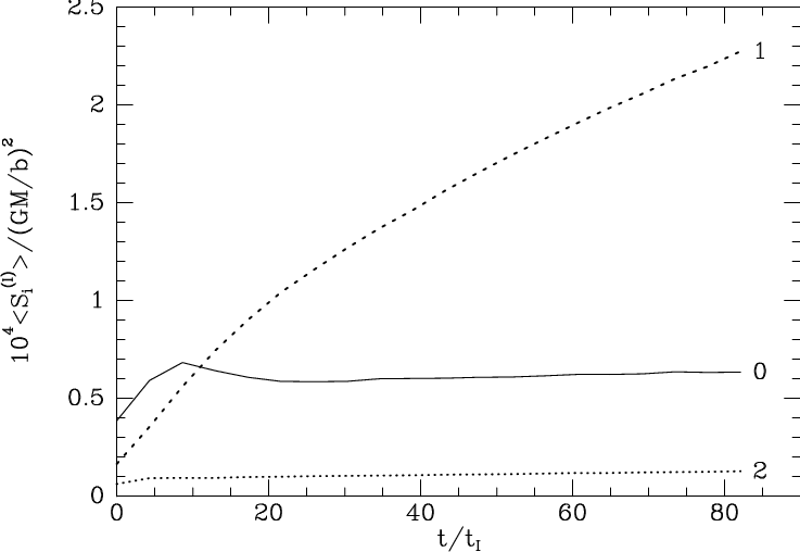
The full, dashed and dotted curves in Fig. 7 show for , respectively, the values of versus time. Initially, the monopole is largest, but it is soon overtaken by the dipole, which continues to rise throughout the simulated period, whereas the monopole stagnates. The quadrupole continues to rise but is much smaller than either the monopole or dipole.
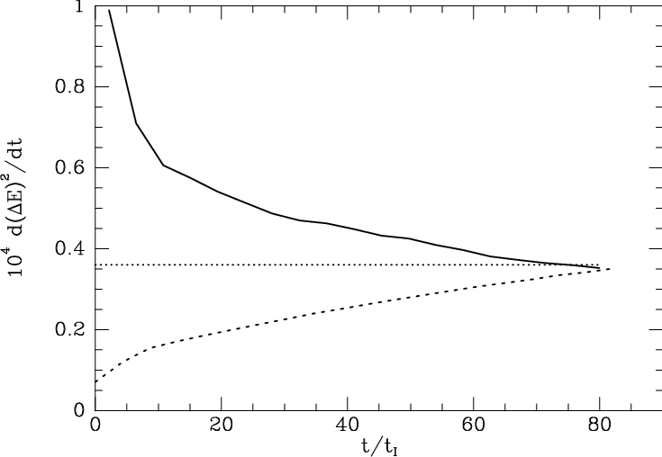
The dashed curve in Fig. 8 shows the resulting estimate from equations (30) and (33) of the rate of growth of when one sets (Appendix A). The full curve in Fig. 8 shows the actual rate of growth of . Although the shapes of the two curves are very different, at the latest time they agree in magnitude better than one has any right to expect given the approximations involved in the computation of the dashed curve.
In Appendix B we quote the formulae for the diffusion coefficients in energy that are yielded by local scattering theory. When the second-order diffusion coefficient is integrated over the isochrone, we find
| (34) |
where . The theory predicts that when we average over all particles, we should find that
| (35) |
The dotted line in Fig. 8 shows this prediction when we adopt .
Interpretation of Fig. 8 is not straightforward. With our chosen value of , local scattering theory yields the correct order of magnitude for but it predicts that the latter should be constant rather than falling. The hypothesis that relaxation is driven by large-scale fluctuations also yields the right order of magnitude for and it correctly predicts that the latter’s value should be a strong function of time rather than constant. Fig. 8, however, suggests that it should be a rising rather than a falling function of time.
Careful consideration reveals that this prediction is likely be an artifact of how we have estimated the right side of equation (26): we have taken the time derivatives of to be their values divided by the characteristic time . This procedure makes sense once the system has settled to an approximate steady state, but initially it is misleading because the fluctuations start from anomalously small amplitudes, so we estimate that they initially have very small time derivatives. Fig. 5 shows clearly that the dipole’s time derivative is initially large, presumably because over-dense regions are falling together, even though its initial magnitude is small. A better estimate of the initial time derivatives of the would be the values they will acquire a time later, divided by . If we liken the large-scale fluctuations to harmonic oscillators, they start with zero amplitude and maximum velocity, and consequently have large time derivatives.
5 Drift velocities in action space
We now use the NBODY6 data to compute the velocities with which stars drift through action space. This is a more sophisticated and direct probe of relaxation than , which is just a global average of the extent to which stars shuffle parallel to a particular direction in action space and takes no account of the fact that most shuffles cancel one another: the distribution function is unchanged when two stars at similar action-space locations exchange energy but is incremented.
H18 show that in the case of a spherical system, action space, which is generically three-dimensional with Cartesian coordinates , can be reduced to the two-dimensional space spanned by , where is the magnitude of the angular momentum vector. The mass density of stars in this space is times
| (36) |
where is the full DF, normalised such that . H18 present plots of the stellar fluxes in two-dimensional action space computed both from the BL equation and from local scattering theory. Their fluxes were normalised to the case of stars in a cluster. In our comparisons below we renormalise their fluxes to clusters of stars.

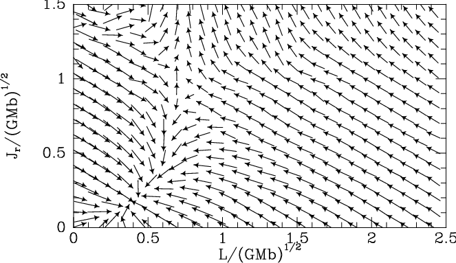

The flux in the plane is associated with a drift velocity
| (37) |
From each snapshot it is straightforward to compute each particle’s value of from its energy and angular momentum because for the isochrone we have an expression for the Hamiltonian
| (38) |
so we can solve for . We divide two-dimensional action space into cells of varying size and we compute the mean of the changes in experienced by stars in each cell during the last half of the simulations, i.e., a time . The drift velocity at the centre of the cell is taken to be
| (39) |
The centre panel of Fig. 9 shows the resulting velocities, while the top and bottom panels show the velocities that correspond to the flux vectors computed by H18 from the BL equation and local scattering theory, respectively. The length of an arrow encodes the speed to the flow via the non-linear scaling
| (40) |
where . The length of an arrow is then a linear function of for and a logarithmic function for .
The three panels differ considerably from one another. The BL vectors in the top panel have a very strong tendency to point towards the origin, while outside the bottom left corner, the local-scattering vectors in the bottom panel point resolutely upward. The NBODY6 vectors are something of a compromise between these two extremes, consistent with the BL and local-scattering vectors capturing opposite halves of what actually happens in a cluster. A feature of the NBODY6 vectors that is captured by the BL vectors is the tendency to converge on a point at low and non-zero . However, the point of convergence lies at substantially larger in the BL panel than in the NBODY6 panel. A striking feature of the NBODY6 panel that is captured by neither the other panels is a strong tendency for vectors to align with lines of constant , which run from upper left to lower right. The NBODY6 and the BL vectors have similar lengths at all points, while the vectors from the local approximation are shorter, especially at low . Thus the local approximation materially under-estimates the speed of relaxation.
Given that H18 included only a handful of resonant pairings, it is inevitable that the BL vectors differ significantly from the NBODY6 vectors. The conflict between the local-scattering and NBODY6 vectors clearly confirms that important physics is missed by local-scattering theory. That physics is the excitation of system-scale oscillations that is made possible by self-gravitation. Thus Fig. 9 further confirms the essential message of H18 that the traditional theory of cluster evolution is highly unsatisfactory.
5.1 Entropy generation
In the central panel Fig. 9, the NBODY6 velocity vectors appear to converge around the point . This convergence implies that in this region is increasing and consequently the entropy density is decreasing. In this subsection we show that notwithstanding the local rise of , the cluster’s entropy is increasing as it must be.
With normalised to unit integral through action space, the entropy of a cluster in equilibrium is
| (41) |
where is a constant with the dimension of Planck’s constant to ensure that the argument of the logarithm is dimensionless. We need to apply this formula to the case of an spherical system, when . As in H18 we define as a third coordinate for action space the cosine of an orbit’s inclination angle, and then we have that . Substituting this expression into equation (41) and integrating over allowed values of we obtain
| (42) |
Differentiating with respect to time, we obtain
| (43) | ||||
| (44) |
where the second equality uses equation (36). Differentiation of the normalisation condition on leads to the conclusion that we can drop the from the square bracket. Then we use the BL equation to eliminate in favour of the flux in space to obtain
| (45) |
The divergence theorem and the fact that in the case of an isotropic system the DF has the form allow us to obtain from this
| (46) | ||||
| (47) |
Given that , this equation states that entropy increases if on average the action-space flux crosses contours of constant outwards.
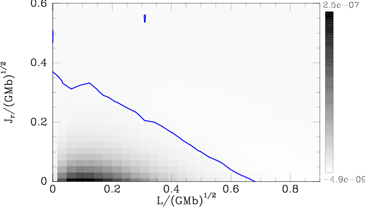
The upper panel of Fig. 10 combines velocity vectors in action space with contours of constant (in red). We see that in much of the space stars flow approximately along lines of constant . In the lower left of the figure there is strong upward movement of stars and thus entropy creation, while in the upper right region stars are moving to lower energy, so entropy is being destroyed. The lower panel of Fig. 10 shows the rate of entropy generation in a grey-scale plot, with the boundary between entropy creation and destruction marked by a blue contour. Entropy is destroyed in most of the depicted part of action space, but the typical creation rates far exceed the destruction rates, so overall net entropy is created, as is physically mandatory.

6 Conclusions
A suite of 10 000 simulations of different realisations of 1000-particle isochrone clusters demonstrates that the neglect of self-gravity by the traditional theory of cluster evolution leads to a seriously incomplete picture of how clusters relax. Over the short durations ( crossing times) of our simulations, self-gravity amplified the original Poisson noise by an order-of magnitude. Figs. 4 and 5 show that the amplification was still some distance from attaining statistical equilibrium by the end of our simulations, so our estimates of the importance of self-gravity must be on the low side. An important implication of this finding is that when a simulations is started by randomly sampling a DF, it starts from an anomalously regular configuration that would not occur in nature. Several crossing times are required for the noise level in the system to settle to a stationary level.
Our experiments were stimulated by the finding of H18 from the BL equation that self-gravity substantially increases the relaxation rate of clusters. Their conclusion was in large measure based on the demonstration of strong excitation by Poisson noise of a cluster’s fundamental dipole mode, a result presaged by the far-sighted work of Weinberg 1993; Weinberg 1998. Our direct-summation N-body simulations confirm that the dipole mode, in which the centre moves in opposition to the halo, is powerfully excited.
We have investigated the extent to which system-scale fluctuations in the gravitational potential can account for diffusion in energy, which is traditionally ascribed to the cumulative effect of stars scattering off other stars. This analysis is tricky because the fluctuations are far from a stationary random process during our brief simulations. However, Fig. 8 provides strong evidence that these fluctuations are at least as effective as star-star scattering in causing the energies of stars to evolve.
Clusters evolve through stars changing their locations in action space. H18 showed that the action space of a spherical system can be reduced to the two-dimensional space spanned by radial action and the magnitude of the angular-momentum vector. Within cells in this space we have determined the mean drift velocity of stars in the N-body simulations and compared these with predictions from the BL equation and local-scattering theory. Fig. 9 shows that the complex action-space flow recovered from the N-body simulations differs from those predicted from the BL equation on the one hand and local-scattering theory on the other in ways that suggest that each of the competing predictions captures roughly a half of the whole picture. The theoretical predictions differ from one another in that the prediction obtained from the BL equation by H18 is known to be incomplete, and is in principle capable of improvement, while that derived from local-scattering theory is definitive and incapable of modification.
Our final conclusion is, therefore, that local-scattering theory is of very limited value. With a judiciously chosen value of its free parameter, , it can be forced to yield a reasonable value for the relaxation rate. It also correctly predicts that stars in the cluster’s halo gain energy at the expense of stars in the core. But it is seriously misleading as regards the basic physics of relaxation and predicts the flow of stars through action space wrongly.
It seems then that to continue work on cluster evolution based on local-scattering theory would be a mistake. Future work should either rely on N-body simulations, or employ the BL equation. For the latter to become a realistic option, one would have to develop a much more efficient code for the computation of diffusion coefficients than that used by H18. the extent to which this is possible is unclear, but it is surely worth a try.
We employed the direct-summation code NBODY6 because we were anxious to exclude any suggestion that our simulations did not handle star-star scattering accurately. If, as now seems likely, relaxation is largely driven by system-scale fluctuations, costly direct-summation could be replaced by a less costly ‘collisionless’ method of force determination, such as tree summation or Fourier transforms. This is another promising direction for future work.
References
- Aarseth (2000) Aarseth S. J., 2000, in Gurzadyan V. G., Ruffini R., eds, The Chaotic Universe NBODY 6: A New Star Cluster Simulation Code. pp 286–287
- Binney & Tremaine (2008) Binney J., Tremaine S., 2008, Galactic Dynamics: Second Edition. Princeton University Press
- Chandrasekhar (1949) Chandrasekhar S., 1949, Reviews of Modern Physics, 21, 383
- Chavanis (2012) Chavanis P.-H., 2012, Physica A, 391, 3680
- Eddington (1916) Eddington A. S., 1916, MNRAS, 76, 572
- Fouvry et al. (2015) Fouvry J. B., Pichon C., Magorrian J., Chavanis P. H., 2015, A&A, 584, A129
- Goldreich & Lynden-Bell (1965) Goldreich P., Lynden-Bell D., 1965, MNRAS, 130, 125
- Hamilton et al. (2018) Hamilton C., Fouvry J.-B., Binney J., Pichon C., 2018, MNRAS, 481, 2041
- Hénon (1960) Hénon M., 1960, Annales d’Astrophysique, 23, 474
- Hénon (1961) Hénon M., 1961, Annales d’Astrophysique, 24, 369
- Heyvaerts (2010) Heyvaerts J., 2010, MNRAS, 407, 355
- Jeans (1915) Jeans J. H., 1915, MNRAS, 76, 70
- Julian & Toomre (1966) Julian W. H., Toomre A., 1966, ApJ, 146, 810
- Kim et al. (2008) Kim E., Yoon I., Lee H. M., Spurzem R., 2008, MNRAS, 383, 2
- King (1966) King I. R., 1966, AJ, 71, 64
- Sellwood & Carlberg (2014) Sellwood J. A., Carlberg R. G., 2014, ApJ, 785, 137
- Spitzer (1987) Spitzer L., 1987, Dynamical evolution of globular clusters. Princeton University Press
- Theuns (1996) Theuns T., 1996, MNRAS, 279, 827
- Toomre (1964) Toomre A., 1964, ApJ, 139, 1217
- Weinberg (1993) Weinberg M. D., 1993, ApJ, 410, 543
- Weinberg (1998) Weinberg M. D., 1998, MNRAS, 297, 101
Appendix A Units
The isochrone has natural length- and time-scales, and . Initial conditions for an N-body simulation of an equilibrium system also define natural length- and time-scales, and . Here we determine the relations between these two systems when the initial conditions are those of an isochrone.
From the initial conditions one can compute the cluster’s potential energy
| (48) |
where is the mass of each of the stars in the cluster. For any given value of , we have
| (49) |
where is a dimensionless vector. NBODY6 rescales the coordinates by choosing such that the expectation value in equation (49) is unity. Then the cluster’s potential energy is
| (50) |
From the initial conditions we can compute the mean-square speed
| (51) |
By the virial theorem, is related to by
| (52) |
With any time, and and
| (53) |
dimensionless times and velocities, the mean-square of the dimensionless velocities is
| (54) |
NBODY6 scales times with chosen such that , so
| (55) |
The potential energy of the isochrone is
| (56) |
Comparing this with equation (50) we find
| (57) |
From equation (55) we have
| (58) |
The period of orbits confined to the core is .

Appendix B Diffusion coefficients in energy
Here we list the formulae from Theuns 1996 and Spitzer 1987 from which we have computed the coefficients that govern diffusion in energy in the approximation of local scattering.
In a system of total mass comprising stars the density of states is
| (59) |
where and is the radius at which vanishes. A related quantity, the density of states weighted by , is given by
| (60) |
With the DF normalised so that , the diffusion coefficients are
| (61) | ||||
| (62) | ||||
| (63) | ||||
| (64) |
Fig. 11 shows the diffusion coefficients. The first-order coefficient changes sign from positive to negative as the binding energy decreases. A useful check on the numerics is provided by the requirement of energy conservation that .