A Survey and Experimental Analysis of Distributed Subgraph Matching
Abstract
Recently there emerge many distributed algorithms that aim at solving subgraph matching at scale. Existing algorithm-level comparisons failed to provide a systematic view to the pros and cons of each algorithm mainly due to the intertwining of strategy and optimization. In this paper, we identify four strategies and three general-purpose optimizations from representative state-of-the-art works. We implement the four strategies with the optimizations based on the common Timely dataflow system for systematic strategy-level comparison. Our implementation covers all representation algorithms. We conduct extensive experiments for both unlabelled matching and labelled matching to analyze the performance of distributed subgraph matching under various settings, which is finally summarized as a practical guide.
Keywords Graph Pattern Matching, Query Optimization, Distributed Processing, Experiments
1 Introduction
Given a query graph and a data graph , subgraph matching is defined as finding all subgraph instances of that are isomorphic to . In this paper, we assume that the query graph and data graph are undirected 11 1 Our implementation can seamlessly handle directed case. simple graphs, and may be unlabelled or labelled. In this work, we mainly focus on unlabelled case given that most distributed algorithms are developed under this setting. We also demonstrate some results of labelled case due to its practical usefulness. Subgraph matching is one of the most fundamental operations in graph analysis, and has been used in a wide spectrum of applications [16, 27, 37, 39, 40].
As subgraph matching problem is in general computationally intractable [47], and data graph nowadays is growing beyond the capacity of one single machine, people are seeking efficient and scalable algorithms in the distributed context. Unless otherwise specified, in this paper we consider a simple hash partition of the graph data, that is the graph is randomly partitioned by vertices, and each vertex’s neighbors will be placed in the same partition.
By treating query vertices as attributes and the matched results as relational tables, we can express subgraph matching via natural joins. The problem is accordingly transformed into seeking optimal join plan, where the optimization goal is typically to minimize the communication cost. In this paper, we focus on an in-depth survey and comparison of representative distributed subgraph matching algorithms that follow such join scheme.
1.1 State-of-the-arts.
In order to solve subgraph matching using join, existing works studied various join strategies, which can be categorized into three classes, namely “Binary-join-based subgraph-growing algorithms" (BinJoin), “Worst-case optimal vertex-growing algorithms" (WOptJoin) and “Shares of Hypercube" (ShrCube). We also include Others category for algorithms that do not clearly belong to the above categories.
BinJoin. The strategy computes subgraph matching via a series of binary joins. It first decomposes the original query graph into a set of join units whose matches can serve the base relation of the join. Then the base relations are joined based on a predefined join order. The BinJoin algorithms differ in the selections of join unit and join order. Typical choices of join unit are star (a tree of depth 1) in [51], TwinTwig (an edge or intersection of two edges) in [35], and clique (a graph whose vertices are mutually connected) in [37]. Most existing algorithms adopt the easier-solving left-deep join order [31] except , which explores the optimality-guaranteed bushy join [31].
WOptJoin. Given as the query vertices, WOptJoin strategy first computes all matches of that can present in the results, then matches of , and so forth until constructing the results. Ngo et al. proposed the worst-case optimal join algorithm GenericJoin [44], based on which Ammar et al. implemented in Timely dataflow system [43] and showed its worst-case optimality [13]. In this paper, we also find out that the BinJoin algorithm (with ‘‘overlapped decomposition’’ 22 2 Decompose the query graph into join units that are allowed to overlap edges) is also a variant of GenericJoin, and is hence worst-case optimal.
ShrCube. ShrCube strategy treats the computation of the query with vertices as an -dimensional hypercube. It partitions the hypercube across workers in the cluster, and then each worker can compute its own share locally with no need of exchanging data. As a result, it typically renders much less communication cost than that of BinJoin and WOptJoin algorithms. adopts the idea of ShrCube for subgraph matching. In order to properly partition the computation without missing results, needs to duplicate each edge in multiple workers. As a result, can almost carry the whole graph in each worker for certain queries [35, 13] and thus scale out poorly.
Others. Shao et al. proposed [50] that processes subgraph matching via breadth-first-style traversal. Staring from an initial query vertex, iteratively expands the partial results by merging the matches of certain vertex’s unmatched neighbors. It has been pointed out in [35] that is actually a variant of . Very recently, Qiao et al. proposed [45] that aims at resolving the “output crisis” by compressing the (intermediate) results. The idea is to first compute the matches of the vertex cover of the query graph, then the remaining vertices’ matches can be compressed as intersection of the vertex cover’s neighbors to avoid costly cartesian product.
Optimizations. Apart from join strategies, existing algorithms also explored a variety of optimizations, some of which are query- or algorithm-specific, while we spotlight three general-purpose optimizations, Batching, TrIndexing and Compression. Batching aims to divide the whole computation into sub-tasks that can be evaluated independently in order to save resource (memory) allocation. TrIndexing precomputes and indices the triangles (3-cycles) of the graph to facilitate pruning. Compression attempts to maintain the (intermediate) results in a compressed form to reduce resource allocation and communication cost.
1.2 Motivations.
In this paper, we survey seven representative algorithms to solve distributed subgraph matching: [51], [12], [50], [35], [37], [45] and [13]. While all these algorithms embody some good merits in theory, existing algorithm-level comparisons failed to provide a systematic view to the pros and cons of each algorithm due to several reasons. Firstly, the prior experiments did not take into consideration the differences of languages and the cost of the systems on which each implementation is based (Table 1). Secondly, some implementations hardcode query-specific optimizations for each query, which makes it hard to judge whether the observed performance is from the algorithmic advancement or hardcoded optimization. Thirdly, all BinJoin and WOptJoin algorithms (more precisely, their implementations) intertwined join strategy with some optimizations of Batching, TrIndexing and Compression. We show in Table 1 how each optimization has been applied in current implementation. For example, only adopted TrIndexing and some query-specific Compression, while considered Batching in general, but TrIndexing only for one specific query (Compression was only discussed in paper, but not implemented). People naturally wonder that “maybe it is better to adopt A strategy with B optimization”, but unfortunately none of existing implementation covers that combination. Last but not least, there misses an important benchmarking of the FullRep strategy, that is to maintain the whole graph in each partition and parallelize embarrassingly [29]. FullRep strategy requires no communication, and it should be the most efficient strategy when each machine can hold the whole graph (the case for most experimental settings nowadays).
| Algorithm | Category | Worst-case Optimality | Platform | Optimizations |
| [51] | BinJoin | No | Trinity [49] | None |
| [12] | ShrCube | N/A | Hadoop [35], Myria [20] | N/A |
| [50] | Others | No | Giraph [4] | None |
| [35] | BinJoin | No | Hadoop | Compression [36] |
| [37] | BinJoin | Yes (Section 6) | Hadoop | TrIndexing, some Compression |
| [45] | Others | N/A | Hadoop | TrIndexing, Compression |
| [13] | WOptJoin | Yes [13] | Timely Dataflow [43] | Batching, specific TrIndexing |
Table 1 summarizes the surveyed algorithms via the category of strategy, the optimality guarantee, and the status of current implementations including the based platform and how the three optimizations are adopted.
1.3 Our Contributions
To address the above issues, we aims at a systematic, strategy-level benchmarking of distributed subgraph matching in this paper. To achieve that goal, we implement all strategies, together with the three general-purpose optimizations for subgraph matching based on the Timely dataflow system [43]. Note that our implementation covers all seven representative algorithms. Here, we use Timely as the base system as it incurs less cost [42] than other popular systems like Giraph [4], Spark [54] and GraphLab [38], so that the system’s impact can be reduced to the minimum.
We implement the benchmarking platform using our best effort based on the papers of each algorithm and email communications with the authors. Our implementation is (1) generic to handle arbitrary query, and does not include any hardcoded optimizations; (2) flexible that can configure Batching, TrIndexing and Compression optimizations in any combination for BinJoin and WOptJoin algorithms; and (3) efficient that are comparable to and sometimes even faster than the original hardcoded implementation. Note that the three general-purpose optimizations are mainly used to reduce communication cost, and is not useful to the ShrCube and FullRep strategies, while we still devote a lot of efforts into their implementations. Aware that their performance heavily depends on the local algorithm, we implement and compare the state-of-the-art local subgraph matching algorithms proposed in [34], [11] (for unlabelled matching), and [16] (for labelled matching), and adopt the best-possible implementation. For ShrCube, we refer to [20] to implement “Hypercube Optimization” for better hypercube sharing.
We make the following contributions in the paper.
(1) A benchmarking platform based on Timely dataflow system for distributed subgraph matching. We implement four distributed subgraph matching strategies (and the general optimizations) that covers seven state-of-the-art algorithms: [51], [12], [50], [35], [37], [45] and [13]. Our implementation is generic to handle arbitrary query, including the labelled and directed query, and thus can guide practical use.
(2) Three general-purpose optimizations - Batching, TrIndexing and Compression. We investigate the literature on the optimization strategies, and spotlight the three general-purpose optimizations. We propose heuristics to incorporate the three optimizations into BinJoin and WOptJoin strategies, with no need of query-specific adjustments from human experts. The three optimizations can be flexibly configured in any combination.
(3) In-depth experimental studies. In order to extensively evaluate the performance of each strategy and the effectiveness of the optimizations, we use data graphs of different sizes and densities, including sparse road network, dense ego network, and web-scale graph that is larger than each machine’s configured memory. We select query graphs of various characteristics that are either from existing works or suitable for benchmarking purpose. In addition to running time, we measure the communication cost, memory usage and other metrics to help reason the performance.
(4) A practical guide of distributed subgraph matching. Through empirical analysis covering the variances of join strategies, optimizations, join plans, we propose a practical guide for distributed subgraph matching. We also inspire interesting future work based on the experimental findings.
1.4 Organizations
. The rest of the paper is organized as follows. Section 2 defines the problem of subgraph matching and introduces preliminary knowledge. Section 3 surveys the representative algorithms, and our implementation details following the categories of BinJoin, WOptJoin, ShrCube and Others. Section 4 investigates the three general-purpose optimizations and devises heuristics of applying them to BinJoin and WOptJoin algorithms. Section 5 demonstrates the experimental results and our in-depth analysis. Section 7 discusses the related works, and Section 8 concludes the whole paper.
2 Preliminaries
2.1 Problem Definition
Graph Notations. A graph is defined as a 3-tuple, , where is the vertex set and is the edge set of , and is a label function that maps each vertex and/or each edge to a label. Note that for unlabelled graph, simply maps all vertices and edges to . For a vertex , denote as the set of neighbors, as the degree of , and as the average and maximum degree, respectively. A subgraph of , denoted , is a graph that satisfies and .
Given , we define induced subgraph as the subgraph induced by , that is , where . We say is a vertex cover of , if , or . A minimum vertex cover is a vertex cover of that contains minimum number of vertices. A connected vertex cover is a vertex cover whose induced subgraph is connected, among which a minimum connected vertex cover, denoted , is the one with the minimum number of vertices.
Data and Query Graph. We denote the data graph as , and let , . Denote a data vertex of id as where . Note that the data vertex has been reordered such that if , then . We denote the query graph as , and let , , and .
Subgraph Matching. Given a data graph and a query graph , we define subgraph isomorphism:
Definition 2.1.
(Subgraph Isomorphism.) Subgraph isomorphism is defined as a bijective mapping such that, (1) , ; (2) , , and . A subgraph isomorphism is called a Match in this paper. With the query vertices listed as , we can simply represent a match as , where for .
The Subgraph Matching problem aims at finding all matches of in . Denote (or when the context is clear) as the result set of in . As prior works [35, 37, 50], we apply symmetry breaking for unlabelled matching to avoid duplicate enumeration caused by automorphism. Specifically, we first assign partial order to the query graph according to [26]. Here, , and means . In unlabelled matching, a match must satisfy the order constraint: , it holds . Note that we do not consider order constraint in labelled matching.
Example 2.1.
In Figure 1, we present a query graph and a data graph . For unlabelled matching, we give the partial order under the query graph. There are three matches: , and . It is easy to check that these matches satisfy the order constraint. Without the order constraint, there are actually four automorphic33 3 Automorphism is an isomorphism from one graph to itself. matches corresponding to each above match [12]. For labelled matching, we use different fillings to represent the labels. There are two matches accordingly - and .

By treating the query vertices as attributes and data edges as relational table, we can write subgraph matching query as a multiway-way join of the edge relations. For example, regardless of label and order constraints, the query of Example 2.1 can be written as the following join
| (1) | ||||
2.2 Timely Dataflow System
Timely is a distributed data-parallel dataflow system [43]. The minimum processing unit of Timely is a worker, which can be simply seen as a process that occupies a CPU core. Typically, one physical multi-core machine can run several workers. Timely follows the shared-nothing dataflow computation model [22] that abstracts the computation as a dataflow graph. In the dataflow graph, the vertex (a.k.a. operator) defines the computing logics and the edges in between the operators represent the data streams. One operator can accept multiple input streams, feed them to the computing, and produce (typically) one output stream. After the dataflow graph for certain computing task is defined, it is distributed to each worker in the cluster, and further translated into a physical execution plan. Based on the physical plan, each worker can accordingly process the task in parallel while accepting the corresponding input portion.
3 Algorithm Survey
We survey the distributed subgraph matching algorithms following the categories of BinJoin, WOptJoin, ShrCube, and Others. We also show that is a variant of GenericJoin [44], and is thus worst-case optimal.
3.1 BinJoin
The simplest BinJoin algorithm uses data edges as the base relation, which starts from one edge, and expands by one edge in each join. For example, to solve the join of Equation 1, a simple plan is shown in Figure 2(a). The join plan is straightforward, but the intermediate results, especially (a 3-path), can be huge.

To improve the performance of BinJoin, people devoted their efforts into: (1) using more complex base relations other than edge; (2) devising better join plan . The base relations represent the matches of a set of sub-structures of the query graph . Each is called a join unit, and it must satisfy and . With the data graph partitioned across the cluster, [37] constrains the join unit to be the structure whose results can be independently computed within each partition (i.e. embarrassingly parallel [29]). It is not hard to see that when each vertex has full access to the neighbors in the partition, we can compute the matches of a -star (a star of leaves) rooted on the vertex by enumerating all -combinations within . Therefore, star is a qualified and indeed widely used join unit.
Given the base relations, the join plan determines an order of processing binary joins. A join plan is left-deep44 4 More precisely it is deep, and can further be left-deep and right-deep. In this paper, we assume that it is left-deep following the prior work [35]. if there is at least a base relation involved in each join, otherwise it is bushy. For example, the join plan in Figure 2(a) is left-deep, and a bushy join plan is shown in Figure 2(b). Note that the bushy plan avoids the expensive in the left-deep plan, and is generally better.
StarJoin. As the name suggests, uses star as the join unit, and it follows the left-deep join order. To decompose the query graph, it first locates the vertex cover of the query graph, and each vertex in the cover and its unused neighbors naturally form a star [51]. A plan for Equation 1 is
where denotes a Star relation (the matches of the star) with as the root, and as the set of leaves.
TwinTwigJoin. Enumerating a -star on a vertex of degree will render cost. We refer star explosion to the case while enumerating stars on a large-degree vertex. Lai et al. proposed [35] to address the issue of by forcing the join plan to use TwinTwig (a star of at most two edges) instead of a general star as the join unit. Intuitively, this would help ameliorate the star explosion by constraining the cost of each join unit from of arbitrary to at most . follows to use left-deep join order. The authors proved that is instance optimal to , that is given any general plan in the left-deep join order, we can rewrite it as an alternative plan that draws no more cost (in the big sense) than the original , where the cost is evaluated based on Erdös-Rényi random graph () model [23]. A plan for Equation 1 is
| (2) | ||||
where denotes a TwinTwig relation with as the root, and as the leaves.
CliqueJoin. hampers star explosion to some extent, but still suffers from the problems of long execution ( rounds) and suboptimal left-deep join plan. resolves the issues by extending in two aspects. Firstly, applies the “triangle partition” strategy (Section 4.2), which enables to use clique, in addition to star, as the join unit. The use of clique can greatly shorten the execution especially when the query is dense, although it still degenerates to when the query contains no clique subgraph. Secondly, exploits the bushy join plan to approach optimality. A plan for Equation 1 is:
| (3) |
where denotes a Clique relation of the involving vertices .
Implementation Details. We implement the BinJoin strategy based on the join framework proposed in [37] to cover , and .
We use power-law random graph () model [21] to estimate the cost as [37], and implement the dynamic programming algorithm [37] to compute the cost-optimal join plan. Once the join plan is computed, we translate the plan into Timely dataflow that processes each binary join using a Join operator. We implement the Join operator following Timely’s official “pipeline” HashJoin example55 5 https://github.com/TimelyDataflow/timely-dataflow/blob/master/examples/hashjoin.rs. We modify it into “batching-style” - the mappers (senders) shuffle the data based on the join key, while the reducers (receivers) maintain the received key-value pairs in a hash table (until mapper completes) for join processing. The reasons that we implement the join as “batching-style” are, (1) its performance is similar to “pipeline” join as a whole; (2) it replays the original implementation in Hadoop; and (3) it favors the Batching optimization (Section 4.1).
3.2 WOptJoin
WOptJoin strategy processes subgraph matching by matching vertices in a predefined order. Given the query graph and as the matching order, the algorithm starts from an empty set, and computes the matches of the subset in the rounds. Denote the partial results after the () round as , and is one of the tuples. In the round, the algorithm expands the results by matching with for iff. , . It is immediate that the candidate matches of , denoted , can be obtained by intersecting the relevant neighbors of the matched vertices as
| (4) |
BiGJoin. adopts the WOptJoin strategy in Timely dataflow system. The main challenge is to implement the intersection efficiently using Timely dataflow. For that purpose, the authors designed the following three operators:
- •
Count: Checking the number of neighbors of each in Equation 4 and recording the location (worker) of the one with the smallest neighbor set.
- •
Propose: Attaching the smallest neighbor set to as .
- •
Intersect: Sending to the worker that maintains each and update .
After intersection, we will expand by pushing into every vertex of .
Implementation Details. We directly use the authors’ implementation [5], but slightly modify the codes to use the common graph data structure. We do not consider the dynamic version of in this paper, as the other strategies currently only support static context. The matching order is determined using a greedy heuristic that starts with the vertex of the largest degree, and consequently selects the next vertex with the most connections (id as tie breaker) with already-selected vertices.
3.3 ShrCube
ShrCube strategy treats the join processing of the query as a hypercube of dimension. It attempts to divide the hypercube evenly across the workers in the cluster, so that each worker can complete its own share without data communication. However, it is normally required that each data tuple is duplicated into multiple workers. This renders a space requirement of for each worker, where is size of the input data, is the number of workers and is a query-dependent parameter. When is close to , the algorithm ends up with maintaining the whole input data in each worker.
MultiwayJoin. applies the ShrCube strategy to solve subgraph matching in one single round. Consider workers in the cluster, a query graph with vertices and , where . Regarding each query vertex , assign a positive integer as bucket number that satisfies . The algorithm then divides the candidate data vertices for evenly into parts via a hash function , where . This accordingly divides the whole computation into shares, each of which can be indiced via an -ary tuple , and is assigned to one worker. Afterwards, regarding each query edge , maps a data edge as , where other than and , each above iterates through , and the edge will be routed to the workers accordingly. Taking triangle query with as an example. According to [12], is an optimal bucket number assignment. Each edge is then routed to the workers as: (1) regarding ; (2) regarding ; (3) regarding , where the above iterates through . Consequently, each data edge is duplicated by roughly times, and by expectation each worker will receive edges. For unlabelled matching, utilizes the partial order of the query graph (Section 2.1) to reduce edge duplication, and details can be found in [12].
Implementation Details. There are two main impact factors of the performance of ShrCube. Firstly, the hypercube sharing by assigning proper for . Beame et al. [15] generalized the problem of computing optimal hypercube sharing for arbitrary query as linear programming. However, the optimal solution may assign fractional bucket number that is unwanted in practice. An easy refinement is to round down to an integer, but it will apparently result in idle workers. Chu et al. [20] addressed this issue via “Hypercube Optimization”, that is to enumerate all possible bucket sequences around the optimal solutions, and choose the one that produces shares (product of bucket numbers) closest to the number of workers. We adopt this strategy in our implementation.
Secondly, the local algorithm. When the edges arrive at the worker, we collect them into a local graph (duplicate edges are removed), and use local algorithm to compute the matches. For unlabelled matching. we study the state-of-the-art local algorithms from “EmptyHeaded” [11] and “DualSim”[34]. “EmptyHeaded” is inspired by Ngo’s worst-case optimal algorithm [44] that decomposes the query graph via “Hyper-Tree Decomposition”, computes each decomposed part using worst-case optimal join and finally glues all parts together using hash join. “DualSim” was proposed by [34] for subgraph matching in the external-memory setting. The idea is to first compute the matches of , then the remaining vertices can be efficiently matched by enumerating the intersection of ’s neighbors. We find out that “DualSim” actually produces the same query plans as “EmptyHeaded” for all our benchmarking queries (Figure 4) except . We implement both algorithms for and “DualSim” performs better than “EmptyHeaded” on the GO, US, GP and LJ datasets (Table 2). As a result, we adopt “DualSim” as the local algorithm for . For labelled matching, we implement “CFLMatch” proposed in [16] that has been shown so far to have the best performance.
Now we let each worker independently compute matches in its local graph. Simply doing so will result in duplicates, so we process deduplication as follows: given a match that is computed in the worker identified by , we can recover the tuple of the matched edge regarding the query edge , then the match is retained if and only if for every . To explain this, let’s consider , and a match for a triangle query , where . It is easy to see that the match will be computed in workers of and , while the match in worker will be eliminated as that matches the query edge can not be hashed to regarding . We can also avoid deduplication by separately maintaing each edge regarding different query edges it stands for, and use the local algorithm proposed in [20], but it results in too many edge duplicates that drain our memory even when processing a medium-size graph.
3.4 Others
PSgL and its implementation. iteratively processes subgraph matching via breadth-first traversal. All query vertices are configured three status, “white” (initialized), “gray” (candidate) and “black” (matched). Denote as the vertex to match in the round. The algorithm starts from matching initial query vertex , and coloring the neighbors as “gray”. In the round, the algorithm applies the workload-aware expanding strategy at runtime, that is to select the to expand among all current “gray” vertices based on a greedy heuristic to minimize the communication cost [49]; the partial results from previous round (specially, ) will be distributed among the workers based on the candidate data vertices that can match ; in the certain worker, the algorithm computes by merging with the matches of the Star formed by and its “white” neighbors , namely ; after is matched, is colored as “black” and its “white” neighbors will be colored as “gray”; essentially, this process is analogous to by processing . Thus, can be seen as an alternative implementation of on Pregel [41]. In this work, we also implement using a Pregel on Timely. Note that we introduce Pregel api to as much as possible replay the implementation of . In fact, it is simply wrapping Timely’s primitive operators such as binary_notify and loop 66 6 https://github.com/frankmcsherry/blog/blob/master/posts/2015-09-21.md, and barely introduces extra cost to the implementation. Our experimental results demonstrate similar findings as prior work [37] that ’s performance is dominated by [37]. Thus, we will not further discuss this algorithm in this paper.
CrystalJoin and its implementation. aims at resolving the “output crisis” by compressing the results of subgraph matching [45]. The authors defined a structure called crystal, denoted . A crystal is a subgraph of that contains two sets of vertices and ( and ), where the induced subgraph is a -clique, and every vertex in connects to all vertices of . We call clique vertices, and the bud vertices. The algorithm first obtains the minimum vertex cover , and then applies the Core-Crystal Decomposition to decompose the query graph into the core and a set of crystals . The crystals must satisfy that , , namely, the clique part of each crystal is a subgraph of the core. As an example, we plot a query graph and the corresponding core-crystal decomposition in Figure 3. Note that in the example, both crystals have an edge (i.e. 2-clique) as the clique part.
With core-crystal decomposition, the computation has accordingly split into three stages:
- 1.
Core computation. Given that itself is a query graph, the algorithm can be recursively applied to compute according to [45].
- 2.
Crystal computation. A special case of crystal is , which is indeed a -clique. Suppose an instance of the is , we can represent the matches w.r.t. as , where denotes the set of vertices that can match . This can naturally be extended to the case with , where any -combinations of the vertices of together with represent a match. This way, the matches of crystals can be largely compressed.
- 3.
One-time assembly. This stage assembles the core instances and the compressed crystal matches to produce the final results. More precisely, this stage is to join the core instance with the crystal matches.
We notice two technical obstacles to implement according to the paper. Firstly, it is worth noting that the core may be disconnected, a case that can produce exponential number of results. The authors applied a query-specific optimization in the original implementation to resolve this issue. Secondly, the authors proposed to precompute the cliques up to certain , while it is often cost-prohibitive to do so in practice. Take UK (Table 2) dataset as an example, the triangles, 4-cliques and 5-cliques are respectively about , and times larger than the graph itself. It is worth noting that the main purpose of this paper is not to study how well each algorithm performs for a specific query, which has its theoretical value, but can barely guide practice. After communicating with the authors, we adapt in the following. Firstly, we replace the core with the induced subgraph of the minimum connected vertex cover . Secondly, instead of implementing as a strategy, we use it as an alternative join plan (matching order) for WOptJoin. According to , we first match , while the matching order inside and outside still follows WOptJoin’s greedy heuristic (Section 3.2). It is worth noting that this adaptation achieves high performance comparable to the original implementation. In fact, we also apply plan to BinJoin, while it does not perform as well as the WOptJoin version, thus we do not discuss this implementation.
FullRep and its implementation. FullRep simply maintains a full replica of the graph in each physical machine. Each worker picks one independent share of computation and solves it using existing local algorithm.
The implementation is straightforward. We let each worker pick its share of computation via a Round-Robin strategy, that is we settle an initial query vertex , and let first worker match with to continue the remaining process, and second worker match with , and so on. This simple strategy already works very well on balancing the load of our benchmarking queries (Figure 4). We use “DualSim” for unlabelled matching and “CFLMatch” for labelled matching as .
3.5 Worst-case Optimality.
Given a query and the data graph , we denote the maximum possible result set as . Simply speaking, an algorithm is worst-case optimal if the aggregation of the total intermediate results is bounded by . Ngo et al. proposed a class of worst-case optimal join algorithm called GenericJoin [44], and we first overview this algorithm.
GenericJoin. Let the join be , where and . Given a vertex subset , let , and for a tuple , denote as ’s projection on . We then show the GenericJoin in Algorithm 1.
if then 1
;
forall do 2
; Return ;
In Algorithm 1, the original join is recursively decomposed into two parts and regarding the disjoint sets and . From line 5, it is clear that will record ’s projection on , thus we have , where is the maximum possible results of the query. Meanwhile, in line 7, the semi-join only retains those w.r.t. that can end up in the join result, which infers that the must also be bounded by the final results. This intuitively explains the worst-case optimality of GenericJoin, while we refer interested readers to [44] for a complete proof.
It is easy to see that is worst-case optimal. In Algorithm 1, we select in line 4 by popping the edge relation in the step. In line 7, the recursive call to solve the semi-join actually corresponds to the intersection process.
Worst-case Optimality of CliqueJoin. Note that the two clique relations in Equation 3 interleave one common edge in the query graph. This optimization, called “overlapping decomposition” [37], eventually contributes to ’s worst-cast optimality. Note that it is not possible to apply this optimization to and . We have the following theorem.
Theorem 3.1.
is worst-case optimal while applying “overlapped decomposition”.
Proof.
We implement using Algorithm 1 in the following. Note that denotes a subgraph of induced by . In line 2, we change the stopping condition to “ is either a clique or a star”. In line 4, the is selected such that is either a clique or a star. Note that by applying the “overlapping decomposition” in , the sub-query of the part must be the -induced graph , and it will also include the edges of , which infers that , and just reflects the semi-join in line 7. Therefore, belongs to GenericJoin, and is thus worst-case optimal. ∎
4 Optimizations
We introduce the three general-purpose optimizations, Batching, TrIndexing and Compression in this section, and how we orthogonally apply them to BinJoin and WOptJoin algorithms. In the rest of the paper, we will use the strategy BinJoin, WOptJoin, ShrCube instead of their corresponding algorithms, as we focus on strategy-level comparison.
4.1 Batching
Let be the partial results that match the given vertices ( for short if follows a given order), and denote the more complete results with . Denote as the tuples in whose projection on equates . Let’s partition into disjoint parts . We define Batching on as the technique to independently process the following sub-tasks that compute . Obviously, .
WOptJoin. Recall from Section 3.2 that WOptJoin progresses according to a predefined matching order . In the round, WOptJoin will Propose on each to compute . It is not hard to see that we can easily apply Batching to the computation of by randomly partitioning . For simplicity, the authors implemented Batching on . Note that in unlabelled matching, which means that we can achieve Batching simply by partitioning the data vertices77 7 Practically, it is more efficient to start from matching the edges instead of the vertices, and we can batch on , where .. For short, we also say the strategy batches on , and call the batching vertex. We follow the same idea to apply Batching to BinJoin algorithms.
BinJoin. While it is natural for WOptJoin to batch on , it is non-trivial to pick such a vertex for BinJoin. Given a decomposition of the query graph , where each is a join unit, we have . If we partition so as to batch on , we correspondingly split the join task, and one of the sub-task is ( is one partition of ). Observe that if there exists a join unit where , we must have , which means have to be fully computed in each sub-task. Let’s consider the example query in Equation 2.
Suppose we batch on , the above join can be divided into the following independent sub-tasks:
It is not hard to see that we will have to re-compute and in all the above sub-tasks. Alternatively, if we batch on , we can avoid such re-computation as and can all be partitioned in each sub-task. Inspired by this, for BinJoin, we come up with the heuristic to apply Batching on the vertex that presents in as many join units as possible. Note that such vertex can only be in the join key, as otherwise it must at least not present in one side of the join. For complex query, we can still have join unit that does not contain any vertex for Batching after applying the above heuristic. In this case, we either re-compute the join unit, or cache it on disk. Another problem caused by this is potential memory burden of the join. Thus, we devise the join-level Batching following the idea of external MergeSort. Specifically, we inject a Buffer-and-Batch operator for the two data streams before they arrive at the Join operator. Buffer-and-Batch functions in two parts:
- •
Buffer: While the operator receives data from the upstream, it buffers the data until reaching a given threshold. Then the buffer is sorted according to the join key’s hash value and spilled to the disk. The buffer is reused for the next batch of data.
- •
Batch: After the data to join is fully received, we read back the data from the disk in a batching manner, where each batch must include all join keys whose hash values are within a certain range.
While one batch of data is delivered to the Join operator, Timely allows us to supervise the progress and hold the next batch until the current batch completes. This way, the internal memory requirement is one batch of the data. Note that such join-level Batching is natively implemented in Hadoop’s “Shuffle” stage, and we replay this process in Timely to improve the scalability of the algorithm.
4.2 Triangle Indexing
As the name suggests, TrIndexing precomputes the triangles of the data graph and indices them along with the graph data to prune infeasible results. The authors of [13] optimized the 4-clique query by using the triangles as base relations to join, which reduces the rounds of join and network communication. In [45], the authors proposed to not only maintain triangles, but all -cliques up to a given . As we mentioned earlier, it incurs huge extra cost of maintaining triangles already, let alone larger cliques.
In addition to the default hash partition, Lai et al. proposed “triangle partition” [37] by also incorporating the edges among the neighbors (it forms triangles with the anchor vertex) in the partition. “Triangle partition” allows BinJoin to use clique as the join unit [37], which greatly reduces the intermediate results of certain queries and improves the performance. “Triangle partition” is in de facto a variant of TrIndexing, which instead of explicitly materializing the triangles, maintains them in the local graph structure (e.g. adjacency list). As we will show in the experiment (Section 5), this will save a lot of space compared to explicit triangle materialization. Therefore, we adopt the “triangle partition” for TrIndexing optimization in this work.
BinJoin. Obviously, BinJoin becomes with TrIndexing, and (or ) otherwise. With worst-case optimality guarantee (Section 3.5), BinJoin should perform much better with TrIndexing, which is also observed in “Exp-1” of Section 5.
WOptJoin. In order to match in the round, WOptJoin utilizes Count, Propose and Intersect to process the intersection of Equation 4. For ease of presentation, suppose connects to the first query vertices , and given a partial match, , we have . In the original implementation, it is required to send via network to all machines that contain each to process the intersection, which can render massive communication cost. In order to reduce the communication cost, we implement TrIndexing for WOptJoin in the following. We first group such that for each group , we have
Because of TrIndexing, we have () maintain in ’s partition. Thus, we only need to send the prefix to ’s machine, and the intersection within can be done locally. We process the grouping using a greedy strategy that always constructs the largest group from the remaining vertices.
Remark 4.1.
The “triangle partition” may result in maintaining a large portion of the data graph in certain partition. Lai et al. pointed out this issue, and proposed a space-efficient alternative by leveraging the vertex orderings [37]. That is, given the partitioned vertex as , and two neighbors and that close a triangle, we place the edge in the partition only when . Although this alteration reduces storage, it may affect the effectiveness of TrIndexing for WOptJoin and the implementations of Batching and Compression for BinJoin algorithms. Take WOptJoin as an example, after using the space-efficient “triangle partition”, we should modify the above grouping as:
Note that the order between query vertices are for symmetry breaking (Section 2.1), and it may not present in certain query, which makes TrIndexing completely useless for WOptJoin.
4.3 Compression
Subgraph matching is a typical combinatorial problem, and can easily produce results of exponential size. Compression aims to maintain the (intermediate) results in a compressed form to reduce resource allocation and communication cost. In the following, when we say “compress a query vertex”, we mean maintaining its matched data vertices in the form of an array, instead of unfolding them in line with the one-one mapping of a match (Definiton 2.1). Qiao et al. proposed to study Compression in general for subgraph matching. As we introduced in Section 3.4, first extracts the minimum vertex cover as uncompressed part, and then it can compress the remaining query vertices as the intersection of certain uncompressed matches’ neighbors. Such Compression leverages the fact that all dependencies (edges) of the compressed part that requires further computation are already covered by the uncompressed part, thus it can stay compressed until the actual matches are requested. inspires a heuristic for doing Compression, that is to compress the vertices whose matches will not be used in any future computation. In the following, we will apply the same heuristic to the other algorithms.
BinJoin. Obviously we can not compress any vertex that presents in the join key. What we need to do is to simply locate the vertices to compress in the join unit, namely star and clique. For star, the root vertex must remain uncompressed, as the leaves’ computation depends on it. For clique, we can only compress one vertex, as otherwise the mutual connection between the compressed vertices will be lost. In a word, we compress two types of vertices for BinJoin, (1) non-key and non-root vertices of a star join unit, (2) one non-key vertex of a clique join unit.
WOptJoin. Based on a predefined join order , we can compress (), if there does not exist () such that . In other words, ’s matches will never be involved in any future intersection (computation). Note that ’s can be trivially compressed. With Compression, when is compressed, we will maintain its matches as an array instead of unfolding it into the prefix like a normal vertex.
5 Experiments
5.1 Experimental settings
Environments. We deploy two clusters for the experiments: (1) a local cluster of 10 machines connected via one 10GBps switch and one 1GBps switch. Each machine has 64GB memory, 1 TB disk and 1 Intel Xeon CPU E3-1220 V6 3.00GHz with 4 physical cores; (2) an AWS cluster of 40 “r5-2xlarge” instances connected via a 10GBps switch, each with 64GB memory, 8 vCpus and 500GB Amazon EBS storage. By default we use the local cluster of 10 machines with 10GBps switch. We run 3 workers in each machine in the local cluster, and 6 workers in the AWS cluster for Timely. The codes are implemented based on the open-sourced Timely dataflow system [8] using Rust 1.32. We are still working towards open-sourcing the codes, and the bins together with their usages are temporarily provided88 8 https://goo.gl/Xp5BrW to verify the results.
Metrics. In the experiments, we measure query time as the slowest worker’s wall clock time from an average of three runs. We allow 3 hours as the maximum running time for each test. We use OT and OOM to indicate a test case runs out of the time limit and out of memory, respectively. By default we will not show the OOM results for clear presentation. We divide into two parts, the computation time and the communication time . We measure as the time the slowest worker spends on actual computation by timing every computing function. We are aware that the actual communication time is hard to measure as Timely overlaps computation and communication to improve throughput. We consider , which mainly records the time the worker waits data from the network channel (a.k.a. communication time). While the other part of communication that overlaps computation is of less interest as it does not affect the query progress. As a result, we simply let in the experiments. We measure the maximum peak memory using Linux’s “time -v” in each machine. We define the communication cost as the number of integers a worker receives during the process, and measure the maximum communication cost among the workers accordingly.
Dataset Formats. We preprocess each dataset as follows: we treat it as a simple undirected graph by removing self-loop and duplicate edges, and format it using “Compressed Sparse Row” (CSR) [3]. We relabel the vertex id according to the degree and break the ties arbitrarily.
Compared Strategies. In the experiments, we implement BinJoin and WOptJoin with all Batching, TrIndexing and Compression optimizations (Section 4). ShrCube is implemented with “Hypercube Optimization” [20], and “DualSim” (unlabelled) [34] and “CFLMatch” (labelled) [16] as local algorithms. FullRep is implemented with the same local algorithms as ShrCube.
Auxiliary Experiments. We have also conducted several auxiliary experiments in the appendix to study the strategies of BinJoin, WOptJoin, ShrCube and FullRep.
5.2 Unlabelled Experiments
Datasets. The datasets used in this experiment are shown in Table 2. All datasets except SY are downloaded from public source, which are indicated by the letter in the bracket (S [9], W [10], D [1]). All statistics are measured as is an undirected graph. Among the datasets, GO is a small dataset to study cases of extremely large (intermediate) result set; LJ, UK and FS are three popular datasets used in prior works, featuring statistics of real social network and web graph; GP is the google plus ego network, which is exceptionally dense; US and EU, on the other end, are sparse road networks. These datasets vary in number of vertices and edges, densities and maximum degree, as shown in Table 2. We synthesize the SY data according to [18] that generates data with real-graph characteristics. Note that the data occupies roughly 80GB space, and is larger than the configured memory of our machine. We synthesize the data because we do not find public accessible data of this size. Larger dataset like Clueweb [2] is available, but it is beyond the processing power of our current cluster.
Each data is hash partitioned (“hash”) across the cluster. We also implement the “triangle partition” (“tri.”) for TrIndexing optimization (Section 4.2). To do so, we use to compute the triangles and send the triangle edges to corresponding partition. We record the time and average number of edges of the two partition strategies. The partition statistics are recorded using the local cluster, except for SY that is processed in the AWS cluster. From Table 2, we can see that is noticeably larger, around 1-10 times larger than . Note that in GP and UK, which either is dense, or must contain a large dense community, the “triangle partition” can maintain a large portion of data in each partition. While compared to complete triangle materialization, “triangle partition” turns out to be much cheaper. For example, the UK dataset contains around 27B triangles, which means each partition in our local cluster should by average take 0.9B triangles (three integers); in comparison, UK’s “triangle partition” only maintains an average of 0.16B edges (two integers) according to Table 2.
We use US, GO and LJ as default datasets in the experiments “Exp-1”, “Exp-2” and “Exp-3” in order to collect useful feedbacks from successful queries, while we may not present certain cases when they do not give new findings.
| Datasets | Name | /mil | /mil | /s | /mil | /s | /mil | ||
| google(S) | GO | 0.86 | 4.32 | 5.02 | 6,332 | 1.53 | 0.28 | 2.31 | 1.23 |
| gplus(S) | GP | 0.11 | 12.23 | 218.2 | 20,127 | 5.57 | 0.80 | 46.5 | 10.68 |
| usa-road(D) | US | 23.95 | 28.85 | 2.41 | 9 | 12.43 | 1.89 | 3.69 | 1.90 |
| livejournal(S) | LJ | 4.85 | 43.37 | 17.88 | 20,333 | 14.25 | 2.81 | 20.33 | 12.49 |
| uk2002(W) | UK | 18.50 | 298.11 | 32.23 | 194,955 | 61.99 | 17.16 | 266.60 | 156.05 |
| eu-road(D) | EU | 173.80 | 342.70 | 3.94 | 20 | 72.96 | 22.47 | 16.98 | 22.98 |
| friendster(S) | FS | 65.61 | 1806.07 | 55.05 | 5,214 | 378.26 | 118.40 | 368.95 | 395.31 |
| Synthetic | SY | 372.00 | 10,000.00 | 53 | 613,461 | 2027 | 493.75 | 5604.00 | 660.61 |
Queries. The queries are presented in Figure 4. We also give the partial order under each query for symmetry breaking. The queries except and are selected based on all prior works [13, 35, 37, 45, 50], while varying in number of vertices, densities, and the vertex cover ratio , in order to better evaluate the strategies from different perspectives. The three queries , and are relatively challenging given their result scale. For example, the smallest dataset GO contains B(illion) , B and B , respectively. For short of space, we record the number of results of each successful query on each dataset in the appendix. Note that and are absent from existing works, while we benchmark considering the importance of path query in practice, and considering the varieties of the join plans.
Exp-1: Optimizations. We study the effectiveness of Batching, TrIndexing and Compression for both BinJoin and WOptJoin strategies, by comparing BinJoin and WOptJoin with their respective variants with one optimization off, namely “without Batching”, “without Trindexing” and “without Compression”. In the following, we use the suffix of “(w.o.b.)”, “(w.o.t.)” and “(w.o.c.)” to represent the three variants. We use the queries and , and the results of US and LJ are shown in Figure 5. By default, we use the batch size of for both BinJoin and WOptJoin (according to [13]) in this experiment, and we reduce the batch size when it runs out of memory, as will be specified.
While comparing BinJoin with BinJoin(w.o.b.), we observe that Batching barely affects the performance of , but severely for on LJ (1800s vs 4000s (w.o.b.) ). The reason is that we still apply join-level Batching for BinJoin(w.o.b.) that dumps the intermediate data to the disk (Section 4.1). While ’s intermediate data includes the massive results of sub-query , which incurs huge amount of disk I/O (US does not have this problem as it produces very few results). We also run without the join-level Batching on LJ, but it fails with OOM. For BinJoin, TrIndexing is a critical optimization, with the observed performance of BinJoin better than that of BinJoin(w.o.t.), especially so on LJ. This is expected as BinJoin(w.o.t.) actually degenerates to . Compression, on the one hand, allows BinJoin to run much faster than BinJoin(w.o.c.) for both queries on LJ, on the other hand, makes it slower on US. The reason is that US is a sparse dataset with few room for Compression, while Compression itself incurs extra cost. We also compare BinJoin with BinJoin(w.o.c.) on the other sparse graph EU, and the results are the same.
For WOptJoin strategy, Batching has little impact to the performance. Surprisingly, after using TrIndexing to WOptJoin, the improvement by average is only around 18%. We do another experiment in the same cluster but using 1GBps switch, which shows WOptJoin is over 6 times faster than WOptJoin(w.o.t.) for both queries on LJ. Note that Timely uses separate threads to buffer received data from the network. Given the same computing speed, a faster network allows the data to be more fully buffered and hence less wait for the following computation. Similar to BinJoin, Compression greatly improves the performance while querying on LJ, but the opposite on US.
Exp-2 Challenging Queries. We study the challenging queries , and in this experiment. We run this experiment using BinJoin, WOptJoin, ShrCube and FullRep, and show the results of US and GO (LJ failed all cases) in Figure 6. Recall that we split the time into computation time and communication time (Section 5.1), here we plot the communication time as gray filling in each bar of Figure 6.
FullRep beats all the other strategies, while ShrCube fails and on GO because of OT. Although ShrCube uses the same local algorithm as FullRep, it spends a lot of time on deduplication (Section 3.3).
We focus on comparing BinJoin and WOptJoin on GO dataset. On the one hand, WOptJoin outperforms BinJoin for and . Their join plans of are nearly the same except that BinJoin relies on a global shuffling on to processing join, while WOptJoin sends the partial results to the machine that maintains the vertex to grow. It is hence reasonable to observe BinJoin’s poorer performance for as shuffling is typically a more costly operation. The case of is similar, so we do not further discuss. On the other hand, even living with costly shuffling, BinJoin still performs better for . Due to the vertex-growing nature, WOptJoin’s “optimal plan” will have to process the costly sub-query . On US dataset, WOptJoin consistently outperforms BinJoin for these queries. This is because that US does not produce massive intermediate results as LJ, thus BinJoin’s shuffling cost consistently dominates.
While processing complex queries like and , we can study varieties of join plans for BinJoin and WOptJoin. First of all, we want the readers to note that BinJoin’s join plan for is different from the optimal plan originally given [37]. The original “optimal” plan computes by joining two tailed triangles (triangle tailed with an edge), while this alternative plan works better by joining the uppers “house-shape” sub-query with the bottom triangle. In theory, the tailed triangle has worse-case bound (AGM bound [44]) of , smaller than the house’s , and BinJoin’s actually favors this plan based on cost estimation. However, we find out that the number of tailed triangles is very close to that of the houses on GO, which renders costly process for the original plan to join two tailed triangles. This indicates insufficiency of both cost estimation proposed in [37] and worst-case optimal bound [13] while computing the join plan, which will be further discussed in Section 6.
Secondly, it is worth noting that we actually report the result of WOptJoin for while using the plan, as it works better than WOptJoin’s original “optimal” plan. For , will first compute , namely the 2-path , thereafter it can compress all remaining vertices and . In comparison, the “optimal” plan can only compress and . In this case, performs better because it configures larger compression. In [45], the authors proved that it renders maximum compression to use the vertex cover as the uncompressed core. However, this may not necessarily result in the best performance, considering that it can be costly to compute the core part. In our experiments, the unlabelled , and labelled are cases that plan performs worse than the original plan (with Compression optimization), where plan does not render strictly larger compression while having to process the costly core part. As a result, we only recommend plan when it leads to strictly larger compression.
The final observation is that the computation time dominates most of the evaluated cases, except BinJoin’s , WOptJoin and ShrCube’s on US. We will further discuss this in Exp-3.
Exp-3 All-Around Comparisons. In this experiment, we run using BinJoin, WOptJoin, ShrCube and FullRep across the datasets GP, LJ, UK, EU and FS. We also run WOptJoin with plan in as it is the only query that renders different plan from plan, and the results show that the performance with plan is consistently better. We report the results in Figure 7, where the communication time is plotted as gray filling. As a whole, among all 35 test cases, FullRep achieves the best 85% completion rate, followed by WOptJoin and BinJoin which complete 71.4% and 68.6% respectively, and ShrCube performs the worst with just 8.6% completion rate.
FullRep typically outperforms the other strategies. Observe that WOptJoin’s performance is often very close to FullRep. The reason is that the WOptJoin’s computing plans for these evaluated queries are similar to “DualSim” adopted by FullRep. The extra communication cost of WOptJoin has been reduced to very low while adopting TrIndexing optimization. While comparing WOptJoin with BinJoin, BinJoin is better for , a clique query (join unit) that requires no join (a case of embarrassingly parallel). BinJoin performs worse than WOptJoin in most other queries, which, as we mentioned before, is due to the costly shuffling. There is an exception - querying on GP - where BinJoin performs better than both FullRep and WOptJoin. We explain this using our best speculation. GP is a very dense graph, where we observe nearly 100 vertices with degree around 10,000. To process , after computing the sub-query , WOptJoin (and “DualSim”) processes the intersection of and (their matches) for . Those larger-degree vertices are now frequently pairing, leading to expensive intersection. In comparison, BinJoin computes by joining the sub-query with . Because both strategies compute , we consider how BinJoin computes . BinJoin first locate the matched vertex of , then matches and among its neighbors, which is generally cheaper than intersecting the neighbors of and to compute . Due to the existence of these high-degree pairs, the cost WOptJoin’s intersection can exceed BinJoin’s shuffling.
We observe that the computation time dominates in most cases as we mentioned in Exp-2. This is trivially true for ShrCube and FullRep, but it may not be clearly so for WOptJoin and BinJoin given that they all need to transfer a massive amount of intermediate data. We investigate this and find out two potential reasons. The first one attributes to Timely’s highly optimized communication component, which allows the computation to overlap communication by using extra threads to receive and buffer the data from the network so that it can be mostly ready for the following computation. The second one is the fast network. We re-run these queries using the 1GBps switch, while the results show the opposite trend that the communication time in turn takes over.
Exp-4 Web-Scale. We run the SY datasets in the AWS cluster of 40 instances. Note that FullRep can not be used as SY is larger than the machine’s memory. We use the queries and , and present the results of BinJoin and WOptJoin (ShrCube fails all cases due to OOM) in Table 3. The results are consistent with the prior experiments, but observe that the gap between BinJoin and WOptJoin while querying is larger. This is because that we now deploy 40 AWS instances, and BinJoin’s shuffling cost increases.
| Queries | BinJoin ()/s | WOptJoin ()/s |
| 8810 (6893) | 1751 (1511) | |
| 76 (75) | 518 (443) |
5.3 Labelled Experiments
We use the LDBC social network benchmarking (SNB) [6] for labelled matching experiment due to the lack of labelled big graphs in the public. SNB provides a data generator that generates a synthetic social network of required statistics, and a document [7] that describes the benchmarking tasks, in which the complex tasks are actually subgraph matching. The join plans of BinJoin and WOptJoin for labelled experiments are generated as unlabelled case, but we use the label frequencies to break tie.
Datasets. We list the datasets and their statistics in Table 4. These datasets are generated using the "Facebook" mode with a duration of 3 years. The dataset’s name, denoted as DG, represents a scale factor of . The labels are preprocessed into integers.
| Name | # Labels | ||||
| DG10 | 29.99 | 176.48 | 11.77 | 4,282,812 | 10 |
| DG60 | 187.11 | 1246.66 | 13.32 | 26,639,563 | 10 |
Queries. The queries, shown in Figure 8, are selected from the SNB’s complex tasks with some adaptions: (1) removing the direction of the edges; (2) removing the edge labels; (3) using one-hop edge for multi-hop edges; (4) removing the “no edge” condition; (5) removing all properties except the node types as labels. For (1) and (2), note that our current implementation can support both cases, and we do the adaptations for consistency and simplicity. For (3) and (4), we adapt them because currently they do not conform with the subgraph matching problem studied in this paper. For (5), it is due to our current limitation in supporting property graph. We leave (3), (4) and (5) as interesting future work.
Exp-5 All-Around Comparisons. We now conduct the experiment using all queries on DG10 and DG60, and present the results in Figure 9. Here we compute the join plans for BinJoin and WOptJoin by using the unlabelled method, but further using the label frequencies to break tie. The gray filling again represents communication time. FullRep outperforms the other strategies in many cases, except that it performs slightly slower than BinJoin for and . This is because that and are join units, and BinJoin processes them locally in each machine as FullRep, and it does not build indices as “CFLMatch” used in FullRep. When comparing to WOptJoin, Among all these queries, we only have that configures different plan (w.r.t. plan) for WOptJoin. The results show that the performance of WOptJoin drops about 10 times while using plan. Note that the core part of is a 5-path of “Psn-City-Cty-City-Psn” with enormous intermediate results. As we mentioned in unlabelled experiments, it may not always be wise to first compute the vertex-cover-induced core.
We now focus on comparing BinJoin and WOptJoin. There are three cases that intrigue us. Firstly, observe that BinJoin performs much better than WOptJoin while querying . The reason is high intersection cost as we discovered on GP dataset in unlabelled matching. Secondly, BinJoin performs worse than WOptJoin in , which again is because of BinJoin’s costly shuffling. The third case is , the most complex query in the experiment. BinJoin performs much better while querying . The bad performance of WOptJoin comes from the long execution plan together with costly intermediate results. The two algorithms all expand the three “Psn”s, and then grow via one of the “City”s to “Cty”, but BinJoin approaches this using one join (a triangle a TwinTwig), while WOptJoin will first expand to “City” then further “Cty”, and the “City” expansion is the culprit of the slower run.
6 Discussions and Future Work.
We discuss our findings and potential future work based on the experiments in Section 5. Eventually, we summarize the findings into a practical guide.
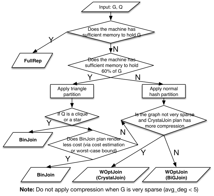
Strategy Selection. FullRep is obviously the preferred choice when the machine can hold the graph data, while both WOptJoin and BinJoin are good alternatives when the graph is larger than the capacity of the machine. For BinJoin and WOptJoin, on one side, BinJoin may perform worse than WOptJoin (e.g. unlabelled , , ) due to the expensive shuffling operation, on the other side, BinJoin can also outperform WOptJoin (e.g. unlabelled and labelled ) while avoiding costly sub-queries due to query decomposition. One way to choose between BinJoin and WOptJoin is to compare the cost of their respective join plans, and select the one with less cost. For now, we can either use cost estimation proposed in [37], or summing the worst-case bound, but none of them consistently gives the best solution, as will be discussed in “Optimal Join Plan”. Alternatively, we refer to “EmptyHeaded” [11] to study a potential hybrid strategy of BinJoin and WOptJoin. Note that “EmptyHeaded” is developed in single-machine setting, and it does not take into consideration the impact of Compression, we hence leave such hybrid strategy in the distributed context as an interesting future work.
Optimizations. Our experimental results suggest always using Batching, using TrIndexing when each machine has sufficient memory to hold “triangle partition”, and using Compression when the data graph is not very sparse (e.g. ). Batching often does not impact performance, so we recommend always using Batching due to the unpredictability of the size of (intermediate) results. TrIndexing is critical for BinJoin, and it can greatly improve WOptJoin by reducing communication cost, while it requires extra storage to maintain “triangle partition”. Amongst the evaluated datasets, each “triangle partition” maintains an average of 30% data in our 10-machine cluster. Thus, we suggest a memory threshold of (half for graph and half for running algorithm) for TrIndexing in a cluster of the same or larger scale. Note that the threshold does not apply to extremely dense graph. Among the three optimizations, Compression is the primary performance booster that improves the performance of BinJoin and WOptJoin by 5 times on average in all but the cases on the very sparse road networks. For such very sparse data graphs, Compression can render more cost than benefits.
Optimal Join Plan. It is challenging to systematically determine the optimal join plans for both BinJoin and WOptJoin. From the experiments, we identify three impact factors: (1) the worst-case bound; (2) cost estimation based on data statistics; (3) favoring the optimizations, especially Compression. All existing works only partially consider these factors, and we have observed sub-optimal join plans in the experiments. For example, BinJoin bases the “optimal” join plan on minimizing the cost estimation, but the join plan does not render the best performance for unlabelled ; WOptJoin follows the worst-case optimality, while it may encounter costly sub-queries for labelled and unlabelled ; focuses on maximizing the compression, while ignoring the facts that the vertex-cover-induced core part itself can be costly to compute. Additionally, there are other impact factors such as the partial orders of query vertices and the label frequencies, which have not been studied in this work due to short of space. It is another very interesting future work to thoroughly study the optimal join plan while considering all above impact factors.
Computation vs. Communication. We argue that distributed subgraph matching nowadays is a computation-intensive task. This claim holds when the cluster configures high-speed network (e.g. GBps), and the data processor can efficiently overlap computation with communication. Note that computation cost (either BinJoin’s join or WOptJoin’s intersection) is lower-bounded by the output size that is equal to the communication cost. Therefore, computation becomes the bottleneck if the network condition is good to guarantee the data to be delivered in time. Nowadays, the bandwidth of local cluster commonly exceeds 10GBps, and the overlapping of computation and communication is widely used in distributed systems (e.g. Spark [54], Flink [17]). As a result, we tend to see distributed subgraph matching as a computation-intensive task, and we advocate future research to devote more efforts into optimizing the computation while considering the following perspectives: (1) the new advancements of hardware, for example the co-processing on GPU in the coupled CPU-GPU architectures [28] and the SIMD programming model on modern CPU [30]; (2) general computing optimizations such as load balancing strategy and cache-aware graph data accessing [53].
A Practical Guide. Based on the experimental findings, we propose a practical guide for distributed subgraph matching in Figure 10. Note that this program guide is based on current progress of the literature, and future work is needed, for examples to study the hybrid strategy and the impact factors of the optimal join plan, before we can arrive at a solid decision-making to choose between BinJoin and WOptJoin.
7 Related Work
Isomorphism-based Subgraph Matching. In the labelled case, Shang et al. [48] used the spanning tree of the query graph to filter infeasible results. Han et al. [27] observed the importance of matching order. In [46], the authors proposed to utilize the symmetry properties in the data graph to compress the results. Bi et al. [16] proposed based on the “core-forest-leaves” matching order, and obtained performance gain by postponing the notorious cartesian product.
The unlabelled case is also known as subgraph listing/enumeration, and due to the gigantic (intermediate) results, people have been either seeking scalable algorithms in parallel, or devising techniques to compress the results. Other than the algorithms studied in this paper (Section 3), Kim et al. proposed the external-memory-based parallel algorithm DualSim [34], which maintains the data graph in blocks on the disk, and matches the query graph by swapping in/out blocks of data to improve I/O efficiency.
Incremental Subgraph Matching. Computing subgraph matching in a continuous context has recently drawn a lot of attentions. Fan et al. [24] proposed incremental algorithm that identifies a portion of the data graph affected by the update regarding the query. The authors in [19] used the join scheme as BinJoin algorithms (Section 3.1). The algorithm maintained a left-deep join tree for the query, with each vertex maintaining a partial query and the corresponding partial results. Then one can compute the incremental answers of each partial query in response to the update, and utilizes the join tree to re-construct the results. Graphflow [33] solved incremental subgraph matching using join, in the sense that the incremental query can be transformed into independent joins, where is the number of query edges. Then they used the worst-case-optimal join algorithm to solve these joins in parallel. Most recently, Kim et al. proposed TurboFlux that maintains data-centric index for incremental queries, which achieves good tradeoff between performance and storage.
Query Languages and Systems. As the increasing demand of subgraph matching in graph analysis, people start to investigate easy-use and highly expressive subgraph matching language. Neo4j introduced Cypher [25], and now people are working on standardizing the semantics of subgraph matching based on Cypher [14]. Gradoop [32] is a system based on Apache Hadoop that translates a Cypher query into a MapReduce job. Aberger et al. proposed EmptyHeaded based on relational semantics for graph processing, in which they leveraged worst-case optimal join algorithm to solve subgraph matching. Arabesque [52] was designed to solve graph mining (continuously computing frequent subgraphs) at scale, while it can be configured for single subgraph query.
8 Conclusions
In this paper, we implement four strategies and three general-purpose optimizations for distributed subgraph matching based on Timely dataflow system, aiming for a systematic, strategy-level comparisons among the state-of-the-art algorithms. Based on thorough empirical analysis, we summarize a practical guide, and we also motivate interesting future work for distributed subgraph matching.
References
- [1] The challenge9 datasets. http://www.dis.uniroma1.it/challenge9.
- [2] The clubweb12 dataset. https://lemurproject.org/clueweb12.
- [3] Compressed sparse row. https://en.wikipedia.org/wiki/Sparse_matrix.
- [4] Giraph. http://giraph.apache.org/.
- [5] The implementation of bigjoin. https://github.com/frankmcsherry/dataflow-join/.
- [6] Ldbc benchmarks. http://ldbcouncil.org/benchmarks.
- [7] The ldbc social network benchmark. https://ldbc.github.io/ldbc_snb_docs/ldbc-snb-specification.pdf.
- [8] The open-sourced timely dataflow system. https://github.com/frankmcsherry/timely-dataflow.
- [9] The snap datasets. http://snap.stanford.edu/data/index.html.
- [10] The webgraph datasets. http://law.di.unimi.it/datasets.php.
- [11] C. R. Aberger, S. Tu, K. Olukotun, and C. Ré. Emptyheaded: A relational engine for graph processing. SIGMOD ’16, pages 431–446.
- [12] F. N. Afrati, D. Fotakis, and J. D. Ullman. Enumerating subgraph instances using map-reduce. In Proc. of ICDE’13, 2013.
- [13] K. Ammar, F. McSherry, S. Salihoglu, and M. Joglekar. Distributed evaluation of subgraph queries using worst-case optimal low-memory dataflows. PVLDB, 11(6):691–704, 2018.
- [14] R. Angles, M. Arenas, P. Barceló, A. Hogan, J. Reutter, and D. Vrgoč. Foundations of modern query languages for graph databases. ACM Comput. Surv., 50(5), 2017.
- [15] P. Beame, P. Koutris, and D. Suciu. Communication steps for parallel query processing. J. ACM, 64(6):40:1–40:58, 2017.
- [16] F. Bi, L. Chang, X. Lin, L. Qin, and W. Zhang. Efficient subgraph matching by postponing cartesian products. SIGMOD ’16, pages 1199–1214, 2016.
- [17] P. Carbone, A. Katsifodimos, Kth, S. Sweden, S. Ewen, V. Markl, S. Haridi, and K. Tzoumas. Apache flink™: Stream and batch processing in a single engine. 38, 01 2015.
- [18] D. Chakrabarti, Y. Zhan, and C. Faloutsos. R-mat: A recursive model for graph mining. In SDM, 2004.
- [19] S. Choudhury, L. B. Holder, G. Chin, K. Agarwal, and J. Feo. A selectivity based approach to continuous pattern detection in streaming graphs. In EDBT, 2015.
- [20] S. Chu, M. Balazinska, and D. Suciu. From theory to practice: Efficient join query evaluation in a parallel database system. SIGMOD ’15, pages 63–78.
- [21] F. R. K. Chung, L. Lu, and V. H. Vu. The spectra of random graphs with given expected degrees. Internet Mathematics, 1(3), 2003.
- [22] D. J. DeWitt and J. Gray. Parallel database systems: The future of database processing or a passing fad? SIGMOD Rec., 19(4):104–112.
- [23] P. Erdos and A. Renyi. On the evolution of random graphs. In Publ. Math. Inst. Hungary. Acad. Sci., 1960.
- [24] W. Fan, J. Li, J. Luo, Z. Tan, X. Wang, and Y. Wu. Incremental graph pattern matching. SIGMOD ’11, pages 925–936, 2011.
- [25] S. Gorka and R. Philip. Improving first-party bank fraud detection with graph databases, 2016.
- [26] J. A. Grochow and M. Kellis. Network motif discovery using subgraph enumeration and symmetry-breaking. In Proc. of RECOMB’07, 2007.
- [27] W.-S. Han, J. Lee, and J.-H. Lee. Turboiso: Towards ultrafast and robust subgraph isomorphism search in large graph databases. In Proc. of SIGMOD’13, 2013.
- [28] J. He, S. Zhang, and B. He. In-cache query co-processing on coupled cpu-gpu architectures. PVLDB, 8(4):329–340, 2014.
- [29] M. Herlihy and N. Shavit. The Art of Multiprocessor Programming. 2008.
- [30] H. Inoue, M. Ohara, and K. Taura. Faster set intersection with simd instructions by reducing branch mispredictions. PVLDB, 8(3):293–304, 2014.
- [31] Y. E. Ioannidis and Y. C. Kang. Left-deep vs. bushy trees: An analysis of strategy spaces and its implications for query optimization. In SIGMOD’91, pages 168–177, 1991.
- [32] M. Junghanns, M. Kiesling, A. Averbuch, A. Petermann, and E. Rahm. Cypher-based graph pattern matching in gradoop. GRADES’17, pages 3:1–3:8.
- [33] C. Kankanamge, S. Sahu, A. Mhedbhi, J. Chen, and S. Salihoglu. Graphflow: An active graph database. SIGMOD ’17, pages 1695–1698.
- [34] H. Kim, J. Lee, S. S. Bhowmick, W.-S. Han, J. Lee, S. Ko, and M. H. Jarrah. Dualsim: Parallel subgraph enumeration in a massive graph on a single machine. SIGMOD ’16, pages 1231–1245, 2016.
- [35] L. Lai, L. Qin, X. Lin, and L. Chang. Scalable subgraph enumeration in mapreduce. PVLDB, 8(10):974–985, 2015.
- [36] L. Lai, L. Qin, X. Lin, and L. Chang. Scalable subgraph enumeration in mapreduce: A cost-oriented approach. The VLDB Journal, 26(3):421–446, June 2017.
- [37] L. Lai, L. Qin, X. Lin, Y. Zhang, L. Chang, and S. Yang. Scalable distributed subgraph enumeration. PVLDB, 10(3):217–228, 2016.
- [38] Y. Low, D. Bickson, J. Gonzalez, C. Guestrin, A. Kyrola, and J. M. Hellerstein. Distributed graphlab: A framework for machine learning and data mining in the cloud. PVLDB, 5(8):716–727, 2012.
- [39] Y. Luo, W. Wang, and X. Lin. Spark: A keyword search engine on relational databases. In ICDE, pages 1552–1555, April 2008.
- [40] Y. Luo, W. Wang, X. Lin, X. Zhou, J. Wang, and K. Li. Spark2: Top-k keyword query in relational databases. IEEE Transactions on Knowledge and Data Engineering, 23(12):1763–1780, Dec 2011.
- [41] G. Malewicz, M. H. Austern, A. J. Bik, J. C. Dehnert, I. Horn, N. Leiser, and G. Czajkowski. Pregel: A system for large-scale graph processing. In Proc. of SIGMOD’10, 2010.
- [42] F. McSherry, M. Isard, and D. G. Murray. Scalability! but at what cost? HOTOS’15, 2015.
- [43] D. G. Murray, F. McSherry, R. Isaacs, M. Isard, P. Barham, and M. Abadi. Naiad: A timely dataflow system. SOSP ’13, pages 439–455, 2013.
- [44] H. Q. Ngo, E. Porat, C. Ré, and A. Rudra. Worst-case optimal join algorithms. J. ACM, 65(3), 2018.
- [45] M. Qiao, H. Zhang, and H. Cheng. Subgraph matching: On compression and computation. PVLDB, 11(2):176–188, 2017.
- [46] X. Ren and J. Wang. Exploiting vertex relationships in speeding up subgraph isomorphism over large graphs. PVLDB, 8(5):617–628, 2015.
- [47] R. Shamir and D. Tsur. Faster subtree isomorphism. In Proceedings of the Fifth Israeli Symposium on Theory of Computing and Systems, pages 126–131, 1997.
- [48] H. Shang, Y. Zhang, X. Lin, and J. X. Yu. Taming verification hardness: An efficient algorithm for testing subgraph isomorphism. PVLDB, 1(1):364–375, 2008.
- [49] B. Shao, H. Wang, and Y. Li. Trinity: A distributed graph engine on a memory cloud. SIGMOD ’13, pages 505–516, 2013.
- [50] Y. Shao, B. Cui, L. Chen, L. Ma, J. Yao, and N. Xu. Parallel subgraph listing in a large-scale graph. In SIGMOD’14, pages 625–636. ACM, 2014.
- [51] Z. Sun, H. Wang, H. Wang, B. Shao, and J. Li. Efficient subgraph matching on billion node graphs. PVLDB, 5(9):788–799, 2012.
- [52] C. H. C. Teixeira, A. J. Fonseca, M. Serafini, G. Siganos, M. J. Zaki, and A. Aboulnaga. Arabesque: A system for distributed graph mining. SOSP ’15, pages 425–440.
- [53] H. Wei, J. X. Yu, C. Lu, and X. Lin. Speedup graph processing by graph ordering. SIGMOD ’16, pages 1813–1828.
- [54] M. Zaharia, M. Chowdhury, M. J. Franklin, S. Shenker, and I. Stoica. Spark: Cluster computing with working sets. In HotCloud’10, pages 10–10.
Appendix A Auxiliary Experiments
Exp-6 Scalability of Unlabelled Matching. We vary the number of machines as 1, 2, 4, 6, 8, 10, and run the unlabelled queries and to see how each strategy (BinJoin, WOptJoin, ShrCube and FullRep) scales out. We further evaluate “Single Thread”, a serial algorithm that is specially implemented for these two queries. According to [42], we define COST of a strategy as the number of workers it needs to outperform the “Single Thread”, which is a comprehensive measurement of both efficiency and scalability. In this experiment, we query and on the popular dataset LJ, and show the results in Figure 11. Note that we only plot the communication and memory consumption for , as follows similar trend. We also test on the other datasets, such as the dense dataset GP, the results are also similar.
All strategies demonstrate reasonable scaling regarding both queries. In terms of COST, note that FullRep is slightly larger than 1, because “DualSim” is implemented in general for arbitrary query, while “SingleThread” uses a hand-tuned implementation. We first analyze the results of . The COST ranking is FullRep (1.6), WOptJoin (2.0), BinJoin (3.1) and ShrCube (3.7). As expected, WOptJoin scales worse than FullRep, while BinJoin scales worse than WOptJoin because shuffling cost is increasing with the number of machines. In terms of memory consumption, it is trivial that FullRep constantly consumes memory of graph size. Due to the use of Batching, both BinJoin and WOptJoin consume very low memory for both queries. Observe that ShrCube consumes much more memory than WOptJoin and BinJoin, even more than the graph data itself. This is because that certain worker may receive more edges (with duplicates) than the graph itself, which increases the peak memory consumption. For communication cost, both BinJoin and WOptJoin demonstrate reasonable drops as the increment of machines. ShrCube renders much less communication as expected, but it shows increasing trend. This is actually a reasonable behavior of ShrCube, as more machines also means more data duplicates. For , the COST ranking is FullRep (2.4), WOptJoin (2.75), BinJoin (3.82) and ShrCube (71.2). Here, ShrCube is dramatically larger, with most time spending on deduplication (Section 3.3). The trend of memory consumption and communication cost of is similar with that of , thus is not further discussed.
Exp-7 Vary Desities for Labelled Matching. Based on DG10, We generate the datasets with densities 10, 20, 40, 80 and 160 by randomly adding edges into DG10. Note that the density-10 dataset is the original DG10 in Table 4. We use the labelled queries and in this experiment, and show the results in Figure 12.
Exp-8 Vary Labels for Labelled Matching. We generate the datasets with number of labels 0, 5, 10, 15 and 20 based on DG10. Note that there are 5 labels in labelled queries and , which are called the target labels. The 10-label dataset is the original DG10. For the one with 5 labels, we will replace each label not in the target labels as one random target label. For the ones with more than 10 labels, we randomly choose some nodes to change their labels into some other pre-defined labels until they contain the required number of labels. For the one with zero label, it degenerates into unlabelled matching, and we use unlabelled version of and instead. The experiment demonstrates the transition from unlabelled matching to labelled matching, where the biggest drop happens for all algorithms. The drops continue with the increment of the number of labels, but less sharply when there are sufficient number of labels (). Observe that when there are very few labels, for example, the 5-label case of , FullRep actually performs worse than BinJoin and WOptJoin. The “CFLMatch” algorithm [16] used by FullRep relies heavily on label-based pruning. Fewer labels render larger candidate set and more recursive calls, resulting in performance drop of FullRep. While fewer labels may enlarge the intermediate results of BinJoin and WOptJoin, but they are relatively small in the labelled case, and does not create much burden for the 10GBps network.
Appendix B Auxiliary Materials
All Query Results. In Table 5, We show the number of results of every successful query on each dataset evaluated in this work. Note that DG10 and DG60 record the labelled queries of .
| Dataset | |||||||||
| GO | 539.58M | 621.18M | 39.88M | 38.20B | 27.80B | 9.28B | 2,168.86B | 330.68B | 1.88T |
| GP | 1.42T | 1.16T | 78.40B | - | - | - | - | - | - |
| US | 1.61M | 21,599 | 90 | 117,996 | 2,186 | 1 | 160.93M | 2,891 | 89 |
| LJ | 51.52B | 76.35B | 9.93B | 53.55T | 44.78T | 18.84T | - | - | - |
| UK | 2.49T | 2.73T | 157.19B | - | - | - | - | - | - |
| EU | 905,640 | 2,223 | 6 | 12,790 | 450 | 0 | 342.48M | 436 | 71 |
| FS | - | 185.19B | 8.96B | - | - | 3.18T | - | - | - |
| SY | - | 834.78B | 5.47B | - | - | - | - | - | - |
| DG10* | 40.14M | 26.76M | 28.73M | 22.59M | 23.08B | 1.49M4 | 47,556 | 42.56M | 10.07M |
| DG60* | 302.41M | 169.86M | 267.38M | 161.69M | 203.33B | 12.44M | 983,370 | 4.14B | 114.19M |