Automatic Coverage Selection for Surface-Based Visual Localization
Abstract
Localization is a critical capability for robots, drones and autonomous vehicles operating in a wide range of environments. One of the critical considerations for designing, training or calibrating visual localization systems is the coverage of the visual sensors equipped on the platforms. In an aerial context for example, the altitude of the platform and camera field of view plays a critical role in how much of the environment a downward facing camera can perceive at any one time. Furthermore, in other applications, such as on roads or in indoor environments, additional factors such as camera resolution and sensor placement altitude can also affect this coverage. The sensor coverage and the subsequent processing of its data also has significant computational implications. In this paper we present for the first time a set of methods for automatically determining the trade-off between coverage and visual localization performance, enabling the identification of the minimum visual sensor coverage required to obtain optimal localization performance with minimal compute. We develop a localization performance indicator based on the overlapping coefficient, and demonstrate its predictive power for localization performance with a certain sensor coverage. We evaluate our method on several challenging real-world datasets from aerial and ground-based domains, and demonstrate that our method is able to automatically optimize for coverage using a small amount of calibration data. We hope these results will assist in the design of localization systems for future autonomous robot, vehicle and flying systems.
I INTRODUCTION
Over the past two decades, robotics and autonomous vehicle systems have increasingly utilized vision sensors, using them to provide critical capabilities including localization. This usage is due in part to the rapid increase in both camera capabilities and computational processing power. Cameras have benefits over other sensors such as radar, providing far more information about the environment including texture and colour. Furthermore, cameras have other advantages including being passive sensing modalities, and the potential to be relatively inexpensive, have small form factors and relatively low power consumption [1].
One of the critical system design considerations for camera-equipped autonomous platforms is the coverage of the cameras, which is affected by a range of factors including the altitude of the platform (for aerial contexts), mounting point (for ground-based vehicles), the camera field of view and the sensor resolution. The choices made with regards to these system properties can also affect other critical system considerations like compute – if a subset of the entire field of view of a camera can be used for effective localization, significant reductions in compute can be achieved.
We addresses this challenge by presenting a novel technique that automatically identifies the trade-off between visual sensor coverage and the performance of a visual localization algorithm. The technique enables automatic selection of the minimum visual sensor coverage required to obtain optimal performance – specifically, optimal localization recall without expending unnecessary compute on processing a larger sensor coverage field than required. We focus our research within the area of vision based surface localization, such as that demonstrated by Kelly et al [2, 3] for warehouse localization, Conte and Doherty [4] in aerial environments and Hover et al [5] in ship hull inspection. We evaluate the proposed method using two surface-based visual localization techniques, on several challenging real-world aerial and ground-based surface datasets, showing that the technique can automatically select the optimal coverage by using calibration data from environments analogous to the deployment environment.
The paper proceeds as follows. Section II summarizes related works, such as surface-based visual localization and procedures for parameter tuning. Sections III and IV provide an overview of the calibration procedure and the experimental setup respectively. The performance of our algorithm and a discussion is presented in Sections V and VI respectively.

II RELATED WORK
In this section we present research related to surface-based visual localization and calibration procedures for parameter tuning. The coverage here is of localization techniques themselves rather than coverage calibration approaches; as to the best of our knowledge we do not believe there is a system that is directly comparable to the technique outlined in this paper.
II-A Surface-Based Visual Localization
In several mobile robotics applications the system moves relative to a surface, such as a drone across the ground, an autonomous vehicle over the road or a submarine relative to a ship’s hull. As a result, several approaches have proposed using the surface that the robot moves relative to as a visual reference map for localization. For example, Kelly et al. thoroughly demonstrated that surface-based visual localization using pixel-based techniques for mobile ground platforms is feasible within warehouse environments with controlled lighting using a monocular camera [2, 3]. Mount et al. also demonstrated this technique can be applied to autonomous vehicles and a road surface, even with day to night image data [6]. Additionally, [7, 8] demonstrate the use of local features for road surface-based visual localization.
Unmanned aerial vehicles (UAVs) regularly use geo-referenced aerial imagery to help alleviate errors caused by GPS outages [4, 9, 10, 11]. For example, Conte et al. demonstrated that they could incorporate feature-based image registration to develop a drift-free state estimation technique for UAVs [4].
The research presented on underwater visual ship hull inspection and navigation further demonstrates that vision based surface localization is feasible even in challenging conditions [5, 12, 13]. There has also been a variety of research into utilizing the surface as the input image stream for visual odometry [14, 15, 16].
All these systems either have a hard-coded empirically tuned parameter defining the amount of the visual sensor to use, or simply use the entire field of view. Therefore, they could be performing unnecessary computations without any performance gains. In contrast, our system automatically selects the optimal visual sensor coverage for maximizing performance while minimizing unnecessary computation.
II-B Calibration Procedures for Visual Localization
The altering of configuration parameters in both deep learning and traditional computer vision algorithms can have a drastic effect on performance [17], such as the the size of images used within appearance-based techniques [18]. This can cause difficulties in successfully making the transition between research and application, as well as between domains [19, 20, 21]. Due to these difficulties, there have been several research areas investigating the development of automatic calibration routines to improve the performance of visual localization alogrithms. Lowry et al. demonstrated online training-free procedures that could determine the probabilistic model for evaluating whether a query image came from the same location as a reference image, even under significant appearance variation [22, 23]. In [24, 25] and [26] Jacobson et al. explored novel calibration methods to automatically optimize sensor threshold parameters for place recognition. Several bodies of work have also used the system’s state estimate to reduce the search space in subsequent iterations, such as that in [16, 15]. In all bodies of work the authors demonstrated that parameter calibration outperformed their state-of-the-art counterparts. However, these techniques typically focused on optimizing a single metric, mainly recall/accuracy, and did not explicitly consider calibrating for both localization performance and computation load in parallel, which is the focus of the research described in this paper.
There has been considerable research into calibration routines to identify spatial and temporal transforms between pre-determined sensor configurations [27, 28, 29, 30, 31, 32]. Significant investigations into using visual sensors to overcome kinematic and control model errors used in robotics platforms has also been an area of key research [33, 34, 35]. These approaches in general have addressed a different set of challenges to those addressed here, instead focusing on the relationship between sensors and robotic platforms or between sensors and other non-localization-based competencies. The automatic selection of hyper-parameters is also related, especially in the deep learning field [17, 36, 37, 38, 39].
III Approach
This section provides an overview of the approach for automatic selection of the sensor coverage required for an optimal combination of visual surface based localization performance and computational requirements. The primary aim and scope of the techniques presented here is to identify the amount of coverage with respect to the sensor field of view and the altitude of a downward-facing camera above the ground plane. The technique requires a small number of aligned training image pairs from an environment analogous to the deployment environment; although we do not attack that particular problem here, there are a multitude of techniques that could potentially be used to bootstrap this data online such as SeqSLAM [18]. We outline the complete calibration procedure in Algorithm 1.
store ground truth and all other localization scores;
end for
fit distribution to all other scores;
calculate OVL between distributions;
store patch radius and OVL in matrix; end for
else
end if
III-A Optimal Coverage Calibration Procedure
The calibration procedure works under the assumption that the similarity of the normal distributions between the ground truth only scores and all scores diverges as sensor coverage, resolution and placement changes. This divergence in distribution similarity is indicative of better single frame matching performance (see Figure 2 for an example). In this paper we use the Overlapping Coefficient (OVL), which is an appropriate measure of distribution similarity [40, 41]. There are various measures for OVL, including Morisita’s [42], Matusita’s [43] and Weitzman’s [44]. We use Weitzman’s measure which is given by,
| (1) |
where and are two normal distributions and is the resulting OVL value. The bounds of the integral, and , are the numerical limits of the technique being utilised. For example, and would be and respectively for NCC. The Overlapping Coefficient was used as the measure of distribution similarity over other methods, such as the Kullback-Leibler divergence, as it decays to zero as two distributions become more dissimilar and because it is symmetric.
Once the OVL value goes below a given threshold there is limited to no performance gains in localization performance. It is at this point we consider the visual sensor coverage to be optimal. As the OVL threshold is most likely between two of the tested calibration OVL values, as in Figure 2, we use linear interpolation to select the point of intersection. If no tested calibration points achieve less than the required OVL we simply take the largest coverage tested. The selection of the optimal operating value hence is given by the following,
| (2) |
where , and are the optimal operating value, and the value above and below the required OVL threshold, , respectively. and are the corresponding OVL values for the tested calibration values and . are all the values tested during calibration.

Within this research our calibration procedure attempts to automatically select the optimal patch radius. We demonstrate the calibration algorithm using two surface-based visual localization techniques, Normalized Cross Correlation (NCC) and local features with sub-patch comparisons. NCC was selected as it has been shown to have relatively good performance within surface-based visual systems, [3, 6, 15, 16]. The local features technique (LFT) is used to demonstrate that the calibration procedure is agnostic to the front-end employed. Figure 3 shows an example of the local feature with sub-patch comparisons technique. This makes the local feature matching more sensitive to translational shifts and is similar to the regional-MAC descriptor outlined in [45] or the patch verification technique described in [46]

IV Experimental Setup
This section describes the experimental setup, including the dataset acquisition and key parameter values. All experiments were performed either on a standard desktop running 64-bit Ubuntu 16.04 and MATLAB-2018b or on Queensland’s University of Technology’s High Performance Cluster running MATLAB-2018b.
IV-A Image Datasets
Datasets were either acquired from aerial photography provided by Nearmap, or from road surface imagery collected using a full-frame Sony A7s DSLR. The datasets are summarised in Table I.
IV-A1 Aerial Datasets
The aerial datasets were acquired by downloading high-resolution aerial photography provided by Nearmap [47]. To ensure suitable dataset variation for validation of our algorithm, the authors collected imagery from forest, field, rural and suburban areas at various altitudes as well as at different qualitative levels of appearance variation. Each Nearmap dataset consists of two pixel aligned images, a reference and a query map. Patches from the query map are compared to the reference map. Figure 4 shows the reference and query maps for each Nearmap dataset.
The Nearmap Datasets 7a to 7c are from the same location with differing altitudes. Similarly, the Nearmap Datasets 8a to 8c are from the same location with the same reference image, but with different query images with various levels of appearance variation (missing buildings and hue variations).
Each Nearmap image was down-sampled to a fixed width while maintaining its aspect ratio. This down-sampling was to increase ease of comparison between different datasets.

IV-A2 Road Surface Datasets
The road surface imagery datasets were acquired using a consumer grade Sony A7s, with a standard lens, capturing video while mounted to the bonnet of a Hyundai iLoad van. Three traversals of the same stretch of road were made, two during the day and one at night. Corresponding day-day (Road Surface 1) and day-night (Road Surface 2) frames with significant overlap were then selected, and the corresponding frames manually pixel aligned. This resulted in two datasets, Road Surface 1 and 2. Both datasets have four pixel aligned images, with day-day and day-night images in datasets 1 and 2 respectively. Similarly to the Nearmap datasets, the first image in each image pair is used as the reference map, while the second is used to generate query patches. Figure 4 shows the four reference and query maps for each Road Surface dataset.
The road surface images were pre-processed, including down-sampling and local patch normalization, to remove the effects of lighting variation and motion blur. This has been shown to improve visual localization performance [18].
| Dataset Name | Dataset Name | Dataset Name |
|---|---|---|
| Nearmap 1 | Nearmap 2 | Nearmap 3 |
| Nearmap 4 | Nearmap 5 | Nearmap 6 |
| Nearmap 7a | Nearmap 7b | Nearmap 7c |
| Nearmap 8a | Nearmap 8b | Nearmap 8c |
| Road Surface 1a | Road Surface 1b | Road Surface 1c |
| Road Surface 2a | Road Surface 2b | Road Surface 2c |
IV-B Parameter Values
The key parameter values are given in Table II. All parameters were empirically determined over a range of test datasets, and then applied to all experimental datasets. As shown by the results, the system was generally able to select a near optimal patch radius across a range of environment appearances and domains (aerial versus ground-based), even with an almost identical set of parameter values.
The selection of the required Overlapping Coefficient () is a trade off between reducing computational overhead at the risk of reduced localization performance and is dependent on the localization front-end. An initial OVL value can be computed by finding the patch radius that achieves high recall on several test datasets. The remaining parameters, which are mostly dependent on the environment domain and sensor parameters, could also be tuned using exemplary data.
| Parameter | Nearmap | Road Surface | Description | |
| NCC | LFT | NCC | ||
| 200 | 400 | 100 | Image Width | |
| N/A | 2 | Patch Normalization Radius | ||
| 0.005 | 0.0225 | 0.005 | Required OVL Threshold | |
| 10 | 5 | True Match Distance Threshold | ||
| 200 | 100 | 200 | Number of Calibration Samples | |
| 1000 | 100 | 1000 | Number of Validation Samples | |
V Experiments and Results
This section presents the results from the various experiments we conducted. To evaluate performance we calculate the recall, as well as a new performance metric which takes into account both recall and computational efficiency. We defined recall as the number of true single frame matches divided by the total number of samples. The second new performance metric is used to test that the calibration procedure does choose the optimal operating point. Optimal performance is defined as maximizing recall with as little computational overhead necessary. This new metric, which we call the max recall to computation efficiency, is given by
| (3) |
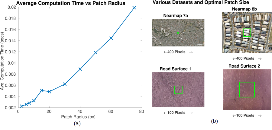
where is the max recall to computation efficiency at patch radius . and are optimal ground truth patch radius for the dataset and all patch radii used during validation. The is used to normalize the distances to be in the range from 0 to 1, while the is used to invert the normalized distances so that a higher value means a higher recall to computation efficiency. The optimal ground truth patch radius, , is defined as the patch radius which achieves 95% of the maximum recall for that dataset. This distance metric naturally encodes the recall and computational efficiency into a single value, and it will punish either unnecessary computational overhead or points that achieve poor relative recall. Patch radius is indicative of computational load, as demonstrated in Figure 7a, which shows that computation time is proportional to patch radius.
V-A Automatic Coverage Selection Evaluation
The first experiment was to investigate the performance of the calibration procedure and test whether it indeed selects the optimal coverage required to maximize localization performance. To evaluate this we ran the calibration routine on a single calibration image that was the same size as and representative of, each Nearmap reference map. We then verified the calibration procedure by testing several patch radii, including the selected patch radius from the calibration routine, on each Nearmap dataset. It should be noted that no image pairs used for calibration are used during validation; and there is no physical overlap between the calibration and validation image pairs in any experiment (see Figure 4).
To validate the calibration procedure we compute the percentage recall and performance metric for several patch radii on the validation image pairs. The results are shown in Figure 5 and 6. Figure 5 shows the results for Nearmap datasets 1-6. Figure 6 shows the results for 7a-c and 8a-c which represent various altitudes and appearance variation.
The Overlap Coefficient for Nearmap 6 does not decay to 0 because the calibration image has an extremely limited amount of unique data (i.e. almost impossible to successfully perform patch localization). Additionally, the validation image does have some unique information which is why 100% percent recall can be achieved.
Figure 7a shows the average computation time is proportional to the patch radius. Additionally, it should be noted that the optimal coverage varies between datasets, as shown in Figure 7b. In Figure 8 we provide a visual example of a traversal through the Nearmap 8b dataset using the optimal patch radius of 30 pixels, as well as a patch radius above and below. As can be seen, the optimal patch radius results in near perfect recall with minimal computational overhead.



V-B Automatic Coverage Selection on a Different Domain
The second experiment investigated how well the automatic selection of the optimal visual coverage worked on a different data domain. For this experiment we used the two road surface datasets. For each dataset, image pair 1 was used for calibration while all four image pairs were used for validation. The results for Road Surface datasets 1 and 2 can be found in Figures 9 and 10 respectively. Please note we validated on all four images, even though image pair 1 is used for training, to allow us to compare results in the following experiment. We will only discuss the results of image pairs 2 to 4 here.
As can be seen, the calibration procedure successfully selects the near optimal patch radius in both Road Surface datasets. The slightly lower max recall to computational efficiency performance of the selected patch radius on the Road Surface 2 dataset is due to the fact that the training data in this case was less representative of the deployment data than the other cases. The higher performance on validation image pairs 2 and 3 compared to validation image pair 4 is probably caused by the fact that the unique features in image pairs 2 and 3 (i.e. cracks, identifiable rocks/patterns) are more evenly distributed throughout the entire image. This means that smaller patches have a higher chance of successful localization in validation image pairs 2 and 3, despite any visual variations (i.e. hue) to the calibration image pair. However, these results still show that the calibration procedure can select an optimal coverage that generalizes to other data (assuming the calibration data is representative of the rest of the dataset).


V-C Automatic Coverage Selection using Multiple Training Images
The previous experiments on Road Surface 2 demonstrate what happens when the training data is not representative of the deployment environment. To mitigate this issue multiple training image pairs can be used. For this experiment we calibrate on image pairs 1 and 2 of the Road Surface 2 dataset and averaged the two optimal patch radii, which were and respectively. This average optimal patch radius, , was then validated on all four images. The results are shown in Figure 11.
The results show that training on multiple images both positively and negatively affects performance. In the case of images 2 and 3 we can see that the selected patch radius is closer to the peak of the max recall to computational efficiency curve. However, for image pairs 1 and 4 we can see that the selected patch radius has resulted in a decrease on the max recall to computational efficiency curve. For image pairs 1 and 4 this shift on the max recall to computational efficiency curve means the overall recall is decreased (i.e. worse localization performance). In contrast, for image pairs 2 and 3, recall is still maximized but computation efficiency has been increased. This suggests the averaging of multiple training image pairs does lead to a better overall performance, since there is only a slight decrease in recall performance for image pairs 1 and 4. However, a more sophisticated approach to selecting the optimal patch radius when using multiple image pairs for training may lead to further improvements; this is an avenue for future investigation.

V-D Automatic Coverage Selection Evaluation using a Feature-Based Localization Approach
To evaluate the generality of the automatic coverage selection process, we performed a second set of experiments with the local feature-based technique previously described as the localization front-end. Due to the extremely challenging appearance change present in much of the Nearmaps datasets, the feature-based approach only produced competitive performance on datasets 4, 7a and 7b, a result mirroring what has been observed in a range of other feature-based localization systems [46]. However, for these environments where the underlying front-end was functional, the calibration routine successfully selected the optimal patch radius in all cases, as can be seen in Figure 12. These results indicate that the coverage selection process can generalize across different localization front-ends.

VI Discussion and Future Work
The presented automatic calibration procedure takes a set of aligned imagery from an environment analogous to the deployment domain, and selects the minimum sensor coverage required to achieve optimal localization performance with minimal compute requirements. Experiments run across both aerial and ground-based surface imagery demonstrated that the approach is able to consistently find this optimal coverage amount, even when it varies hugely across application domains and environments.
There are a range of enhancements and extensions that can be pursued in future work. The first is to investigate the potential use of appearance-invariant visual localization algorithms to generate the aligned training data “on the fly” at deployment time, removing the need to have training data beforehand and allowing for continuous online calibration. The second is to investigate other criteria for finding the optimal operating point beyond the implementation used in this research – such as defining a “plateau” threshold in the overlap coefficient curve at which point performance gains diminish with increased sensor coverage.
Thirdly, we have investigated sensor coverage of the environment here but not other properties like sensor resolution. Such properties could likely be optimized through a similar process to the one used here for coverage. Fourthly, the technique has been demonstrated to be agnostic to surface-based visual localization techniques – it will be interesting to investigate how it performs on other visual localization systems, for example forward-facing cameras. Additionally, there may be absolute criteria that can be used to determine the optimal coverage for a given environment, again removing the requirement to have training data with aligned imagery. Finally, while the required OVL value is dependent on the localization technique, the heuristically determined OVL thresholds selected appear to be robust across a range of very different datasets and domains, including various image sizes and pre-processing steps. However, a sensitivity analysis would be worth investigating. Additionally, further work into the automatic selection of parameter values as well as a probabilistic interpretation of how to select the OVL value could draw on existing methods, such as [23, 24]
Choosing the right camera configuration with respect to mounting and field of view, as well as the operating altitude of an unmanned aerial vehicle, is a critical process both during system design and during deployment operations. We hope that the research presented here will provide an additional tool with which to address these challenges.
ACKNOWLEDGMENT
James Mount and Michael Milford are with the Australian Centre for Robotic Vision at the Queensland University of Technology. This work was supported by an ARC Centre of Excellence for Robotic Vision Grant CE140100016, an Australian Research Council Future Fellowship FT140101229 to Michael Milford and an Australia Postgraduate Award and a QUT Excellence Scholarship to James Mount. The authors also appreciate the support and computing resources provided by QUT’s High Performance Centre (HPC).
References
- [1] M. Milford, W. Scheirer, E. Vig, A. Glover, O. Baumann, J. Mattingley, and D. Cox, “Condition-invariant, top-down visual place recognition,” in 2014 IEEE International Conference on Robotics and Automation (ICRA). IEEE, 2014, pp. 5571–5577.
- [2] A. Kelly, “Mobile robot localization from large-scale appearance mosaics,” The International Journal of Robotics Research, vol. 19, no. 11, pp. 1104–1125, 2000. [Online]. Available: http://dx.doi.org/10.1177/02783640022067896
- [3] A. Kelly, B. Nagy, D. Stager, and R. Unnikrishnan, “Field and service applications - an infrastructure-free automated guided vehicle based on computer vision - an effort to make an industrial robot vehicle that can operate without supporting infrastructure,” IEEE Robotics Automation Magazine, vol. 14, no. 3, pp. 24–34, Sept 2007.
- [4] G. Conte and P. Doherty, “Vision-based unmanned aerial vehicle navigation using geo-referenced information,” EURASIP Journal on Advances in Signal Processing, vol. 2009, p. 10, 2009.
- [5] F. S. Hover, R. M. Eustice, A. Kim, B. Englot, H. Johannsson, M. Kaess, and J. J. Leonard, “Advanced perception, navigation and planning for autonomous in-water ship hull inspection,” The International Journal of Robotics Research, vol. 31, no. 12, pp. 1445–1464, 2012.
- [6] J. Mount and M. Milford, “Image rejection and match verification to improve surface-based localization,” in Australasian Conference on Robotics and Automation (ACRA), 2017.
- [7] K. Kozak and M. Alban, “Ranger: A ground-facing camera-based localization system for ground vehicles,” in 2016 IEEE/ION Position, Location and Navigation Symposium (PLANS), April 2016, pp. 170–178.
- [8] L. Zhang, A. Finkelstein, and S. Rusinkiewicz, “High-precision localization using ground texture,” CoRR, vol. abs/1710.10687, 2017. [Online]. Available: http://arxiv.org/abs/1710.10687
- [9] D.-G. Sim, R.-H. Park, R.-C. Kim, S. U. Lee, and I.-C. Kim, “Integrated position estimation using aerial image sequences,” IEEE Trans. Pattern Anal. Mach. Intell., vol. 24, pp. 1–18, 2002.
- [10] F. Caballero, L. Merino, J. Ferruz, and A. Ollero, “Vision-based odometry and slam for medium and high altitude flying uavs,” Journal of Intelligent and Robotic Systems, vol. 54, no. 1-3, pp. 137–161, 2009.
- [11] R. Madison, G. Andrews, P. DeBitetto, S. Rasmussen, and M. Bottkol, “Vision-aided navigation for small uavs in gps-challenged environments,” in AIAA Infotech@ Aerospace 2007 Conference and Exhibit, 2007, p. 2986.
- [12] A. Kim and R. M. Eustice, “Real-time visual slam for autonomous underwater hull inspection using visual saliency,” IEEE Transactions on Robotics, vol. 29, no. 3, pp. 719–733, June 2013.
- [13] P. Ozog and R. M. Eustice, “Toward long-term, automated ship hull inspection with visual slam, explicit surface optimization, and generic graph-sparsification,” in 2014 IEEE International Conference on Robotics and Automation (ICRA), May 2014, pp. 3832–3839.
- [14] M. Dille, B. Grocholsky, and S. Singh, “Outdoor downward-facing optical flow odometry with commodity sensors,” in Field and Service Robotics. Springer, 2010, pp. 183–193.
- [15] N. Nourani-Vatani and P. V. K. Borges, “Correlation-based visual odometry for ground vehicles,” Journal of Field Robotics, vol. 28, no. 5, pp. 742–768, 2011.
- [16] M. O. Aqel, M. H. Marhaban, M. I. Saripan, and N. B. Ismail, “Adaptive-search template matching technique based on vehicle acceleration for monocular visual odometry system,” IEEJ Transactions on Electrical and Electronic Engineering, vol. 11, no. 6, pp. 739–752, 2016.
- [17] J. S. Bergstra, R. Bardenet, Y. Bengio, and B. Kégl, “Algorithms for hyper-parameter optimization,” in Advances in neural information processing systems, 2011, pp. 2546–2554.
- [18] M. J. Milford and G. F. Wyeth, “Seqslam: Visual route-based navigation for sunny summer days and stormy winter nights,” in 2012 IEEE International Conference on Robotics and Automation. IEEE, 2012, pp. 1643–1649.
- [19] A. Jacobson, F. Zeng, D. Smith, N. Boswell, T. Peynot, and M. Milford, “Semi-supervised slam: Leveraging low-cost sensors on underground autonomous vehicles for position tracking,” in 2018 IEEE/RSJ International Conference on Intelligent Robots and Systems (IROS). IEEE, 2018, pp. 3970–3977.
- [20] F. Zeng, A. Jacobson, D. Smith, N. Boswell, T. Peynot, and M. Milford, “I2-s2: Intra-image-seqslam for more accurate vision-based localisation in underground mines,” in Australasian Conference on Robotics and Automation (ACRA), 2018.
- [21] ——, “Enhancing underground visual place recognition with shannon entropy saliency,” in Australasian Conference on Robotics and Automation (ACRA), 2017.
- [22] S. M. Lowry, G. F. Wyeth, and M. J. Milford, “Towards training-free appearance-based localization: probabilistic models for whole-image descriptors,” in 2014 IEEE international conference on robotics and automation (ICRA). IEEE, 2014, pp. 711–717.
- [23] S. Lowry and M. J. Milford, “Building beliefs: Unsupervised generation of observation likelihoods for probabilistic localization in changing environments,” in 2015 IEEE/RSJ International Conference on Intelligent Robots and Systems (IROS). IEEE, 2015, pp. 3071–3078.
- [24] A. Jacobson, Z. Chen, and M. Milford, “Online place recognition calibration for out-of-the-box slam,” in 2015 IEEE/RSJ International Conference on Intelligent Robots and Systems (IROS). IEEE, 2015, pp. 1357–1364.
- [25] ——, “Autonomous multisensor calibration and closed-loop fusion for slam,” Journal of Field Robotics, vol. 32, no. 1, pp. 85–122, 2015.
- [26] ——, “Autonomous movement-driven place recognition calibration for generic multi-sensor robot platforms,” in 2013 IEEE/RSJ International Conference on Intelligent Robots and Systems. IEEE, 2013, pp. 1314–1320.
- [27] W. Maddern, A. Harrison, and P. Newman, “Lost in translation (and rotation): Rapid extrinsic calibration for 2d and 3d lidars,” in 2012 IEEE International Conference on Robotics and Automation. IEEE, 2012, pp. 3096–3102.
- [28] P. Furgale, J. Rehder, and R. Siegwart, “Unified temporal and spatial calibration for multi-sensor systems,” in 2013 IEEE/RSJ International Conference on Intelligent Robots and Systems. IEEE, 2013, pp. 1280–1286.
- [29] J. Kelly and G. S. Sukhatme, “Visual-inertial sensor fusion: Localization, mapping and sensor-to-sensor self-calibration,” The International Journal of Robotics Research, vol. 30, no. 1, pp. 56–79, 2011.
- [30] D. Scaramuzza, A. Harati, and R. Siegwart, “Extrinsic self calibration of a camera and a 3d laser range finder from natural scenes,” in 2007 IEEE/RSJ International Conference on Intelligent Robots and Systems. IEEE, 2007, pp. 4164–4169.
- [31] G. Pandey, J. R. McBride, S. Savarese, and R. M. Eustice, “Automatic extrinsic calibration of vision and lidar by maximizing mutual information,” Journal of Field Robotics, vol. 32, no. 5, pp. 696–722, 2015.
- [32] S. Weiss, M. W. Achtelik, S. Lynen, M. Chli, and R. Siegwart, “Real-time onboard visual-inertial state estimation and self-calibration of mavs in unknown environments,” in 2012 IEEE International Conference on Robotics and Automation. IEEE, 2012, pp. 957–964.
- [33] Y. Meng and H. Zhuang, “Autonomous robot calibration using vision technology,” Robotics and Computer-Integrated Manufacturing, vol. 23, no. 4, pp. 436–446, 2007.
- [34] M. Švaco, B. Šekoranja, F. Šuligoj, and B. Jerbić, “Calibration of an industrial robot using a stereo vision system,” Procedia Engineering, vol. 69, pp. 459–463, 2014.
- [35] G. Du and P. Zhang, “Online robot calibration based on vision measurement,” Robotics and Computer-Integrated Manufacturing, vol. 29, no. 6, pp. 484–492, 2013.
- [36] J. Bergstra and Y. Bengio, “Random search for hyper-parameter optimization,” Journal of Machine Learning Research, vol. 13, no. Feb, pp. 281–305, 2012.
- [37] C. Thornton, F. Hutter, H. H. Hoos, and K. Leyton-Brown, “Auto-weka: Combined selection and hyperparameter optimization of classification algorithms,” in Proceedings of the 19th ACM SIGKDD international conference on Knowledge discovery and data mining. ACM, 2013, pp. 847–855.
- [38] R. Bardenet, M. Brendel, B. Kégl, and M. Sebag, “Collaborative hyperparameter tuning,” in International conference on machine learning, 2013, pp. 199–207.
- [39] C. Gold, A. Holub, and P. Sollich, “Bayesian approach to feature selection and parameter tuning for support vector machine classifiers,” Neural Networks, vol. 18, no. 5-6, pp. 693–701, 2005.
- [40] H. F. Inman and E. L. Bradley Jr, “The overlapping coefficient as a measure of agreement between probability distributions and point estimation of the overlap of two normal densities,” Communications in Statistics-Theory and Methods, vol. 18, no. 10, pp. 3851–3874, 1989.
- [41] B. Reiser and D. Faraggi, “Confidence intervals for the overlapping coefficient: the normal equal variance case,” Journal of the Royal Statistical Society: Series D (the Statistician), vol. 48, no. 3, pp. 413–418, 1999.
- [42] M. Morisita, “Measuring of interspecific association and similarity between communities,” Mem. Fac. Sci. Kyushu Univ. Series E, vol. 3, pp. 65–80, 1959.
- [43] K. Matusita et al., “Decision rules, based on the distance, for problems of fit, two samples, and estimation,” The Annals of Mathematical Statistics, vol. 26, no. 4, pp. 631–640, 1955.
- [44] M. S. Weitzman, Measures of overlap of income distributions of white and Negro families in the United States. US Bureau of the Census, 1970, vol. 22.
- [45] G. Tolias, R. Sicre, and H. Jégou, “Particular object retrieval with integral max-pooling of cnn activations,” arXiv preprint arXiv:1511.05879, 2015.
- [46] M. Milford, E. Vig, W. Scheirer, and D. Cox, “Vision-based simultaneous localization and mapping in changing outdoor environments,” Journal of Field Robotics, vol. 31, no. 5, pp. 780–802, 2014. [Online]. Available: https://onlinelibrary.wiley.com/doi/abs/10.1002/rob.21532
- [47] “Nearmap - aerial photography,” https://www.nearmap.com.au/, accessed: 2019-01-24.