USTC-ICTS-19-15 A New Littlest Seesaw Model

The Standard Model (SM) has been well established by the discovery of the Higgs boson. However, the discovery of neutrino oscillations implies that neutrinos have masses and there are flavour mixing in lepton sector. Non-zero neutrino masses open up a window to the new physics beyond SM. However, the origin of neutrino mass generation and the flavour mixings in quark and lepton sectors are still unknown [1, 2]. In order to elegantly generate the tiny neutrino mass, the most appealing theory seems to be type I seesaw mechanism involving heavy right-handed Majorana neutrinos [3, 4, 5].

The type I seesaw mechanism can qualitatively explain the smallness of neutrino masses through the heavy right-handed neutrinos. However, if one doesn’t make other assumptions, the seesaw model with three right-handed neutrinos (RHN) contains too many parameters to make any particular predictions for neutrino mass and mixing. As we know, the idea of sequential dominance (SD) [6, 7] of right-handed neutrinos is an effective method to produce the mass hierarchy between the two mass squared differences $\Delta m^{2}_{21}$ and $\Delta m^{2}_{31}$ [8], it requires that the mass spectrum of heavy Majorana neutrinos is strongly hierarchical, i.e. $M_{\text{atm}}\ll M_{\text{sol}}\ll M_{\text{dec}}$. It arises from the proposal that a dominant heavy right-handed (RH) neutrino is mainly responsible for the atmospheric neutrino mass, a heavier subdominant RH neutrino for the solar neutrino mass, and a possible third largely decoupled RH neutrino for the lightest neutrino mass. It leads to an effective two right-handed neutrino (2RHN) model  [9, 10]. This simple idea leads to equally simple predictions which makes the scheme falsifiable. Indeed, the litmus test of such SD is a very light (or massless) neutrino. These predictions will be tested soon. In order to further increase predictive power of the minimal seesaw mechanism, various proposals have been suggested, such as postulating one [11] or two [10] texture zeros in the neutrino Yukawa coupling. The models with two texture zero are excluded by the present data for normal ordering neutrino masses [12, 13, 14].

A very predictive minimal seesaw model with one texture zero is the so-called CSD($n$) model  [15, 16, 17, 18, 19, 20, 21, 22, 23, 24], where the parameter $n$ was usually assumed to be a positive integer. The CSD($n$) scheme assumes that the two columns of the Dirac neutrino mass matrix are proportional to $(0,1,-1)$ and $(1,n,2-n)$ respectively in the RHN diagonal basis. As a consequence, the lepton mixing matrix is predicted to be TM1 pattern, the neutrino masses are normal ordering and the lightest neutrino is massless with $m_{1}=0$. At present only the CSD($3$) (also called Littlest Seesaw model) [17, 18, 19, 20, 21] and CSD($4$) models [22, 23] can give rise to phenomenologically viable predictions for lepton mixing parameters and the two neutrino mass squared differences $\Delta m^{2}_{21}$ and $\Delta m^{2}_{31}$.

It has been shown that CSD($n$) can be enforced by a residual symmetry of $S_{4}$ [19] in the semi-direct approach where different residual flavour symmetries $G_{l}=Z^{T}_{3}$ and $G_{\nu}=Z_{2}^{SU}$ are assumed in the charged lepton and neutrino sectors. However, it was not possible to identify any residual CP symmetry for CSD($n$) in the semi-direct approach. This means that the parameter $n$ of CSD($n$), which is usually assumed to be integer valued, could in fact be a complex number in general. In order to preserve the predictions of CSD($n$), we would like to fix the parameter $n$ to be real (although not necessarily an integer). This suggests that we should seek to somehow use residual CP symmetry, even though it is not possible within the semi-direct approach.

In the past years, discrete flavour symmetry has been combined with generalized CP symmetry to provide a powerful framework to explain the lepton mixing angles and predict leptonic CP violation phases [25, 26, 27, 28, 29, 30, 31, 32, 33, 34, 35, 36, 37, 38, 39, 40, 41, 42, 43, 44, 45, 46, 47, 48, 49, 50, 51, 52, 53, 54, 55, 56, 57]. Furthermore, a simultaneous description of quark and lepton flavour mixing and CP violation can be achieved through spontaneous breaking of a discrete family symmetry and CP symmetry [52, 53, 54]. Since the generalized CP symmetry may play a critical role in understanding the flavour puzzle of SM, recently we extended the widely studied direct model of discrete flavour symmetry [1] to propose a new predictive neutrino mass model building scheme for the minimal seesaw model with two right-handed neutrinos called the tri-direct CP approach [58, 59].

The basic idea of the tri-direct CP approach is that the Yukawa interactions associated with each of the two right-handed neutrinos preserve different residual flavour and CP symmetries, and the charged lepton sector also has a different residual flavour symmetry. As a consequence, the flavour and generalized CP symmetry $G_{f}\rtimes H_{CP}$ is spontaneously broken down to $G_{l}$, $G_{\text{atm}}\rtimes H^{\text{atm}}_{CP}$ and $G_{\text{sol}}\rtimes H^{\text{sol}}_{CP}$ in the charged lepton, “atmospheric” and “solar” right-handed neutrino sectors, respectively [58]. Here $G_{l}$ is an abelian subgroup of $G_{f}$ and it allows the distinction of three generations of charged leptons as usual direct model. The residual subgroups $G_{\text{atm}}\rtimes H^{\text{atm}}_{CP}$ and $G_{\text{sol}}\rtimes H^{\text{sol}}_{CP}$ fix the alignments associated with each right-handed neutrino. We have performed a comprehensive analysis of lepton mixing patterns which can be obtained from the flavour group $S_{4}$ and CP symmetry in the tri-direct CP approach in a model independent fashion [59]. The model construction along the tri-direct CP approach was also illustrated [58, 59]. In the minimal seesaw model, a phenomenologically viable pattern of lepton mixing and neutrino masses can also be obtained from the breaking of $A_{5}$ flavour symmetry into three different subgroups in the charged lepton, atmospheric neutrino and solar neutrino sectors [60].

It is remarkable that the original Littlest Seesaw model for CSD(3) can be reproduced from the tri-direct CP approach [58, 59], if the $S_{4}$ flavour symmetry and CP symmetry are broken to the remnant symmetries $Z^{T}_{3}$, $Z^{U}_{2}\times H^{\text{atm}}_{CP}$ and $Z_{2}^{SU}\times H^{\text{sol}}_{CP}$ in the charged lepton sector, the atmospheric sector and the solar neutrino sector, respectively, corresponding to the $\mathcal{N}_{1}$ case. In this case, one row of the neutrino Dirac mass matrix is proportional to $(0,-1,1)$ and the other row is proportional to $(1,2-x,x)$, where $x$ is enforced to be a real parameter by the residual symmetry, thereby overcoming the previous problem where it could be complex in general. Then the light neutrino mass matrix is determined to be¹¹ 1 Note that the seesaw mechanism results in a light effective Majorana mass matrix was defined in the convention ${\cal L_{\rm eff}}=-\frac{1}{2}\overline{\nu_{L}^{c}}m_{\nu}\nu_{L}+\text{h.c.}$ Also note that here the second entries of the vacuum alignments which enter the Dirac mass matrix are multiplied by minus one as compared to the usual Littlest Seesaw convention. [59]

where an overall phase has been neglected, $m_{a}$, $m_{s}$, $\eta$ and $x$ are four real free parameters. In a concrete model, the parameters $x$ and $\eta$ could be fixed to certain values through the technique of vacuum alignment [58, 59]. For example, CSD(3) corresponding to $x=3$ and $\eta=2\pi/3$, can be achieved within the $\mathcal{N}_{1}$ case. Then all three mixing angles, two CP phases and three neutrino masses only depend on two real parameters $m_{a}$ and $m_{s}$ which can be determined by the mass squared differences $\Delta m^{2}_{21}\equiv m^{2}_{2}-m^{2}_{1}$ and $\Delta m^{2}_{31}\equiv m^{2}_{3}-m^{2}_{1}$ precisely measured in neutrino oscillation experiments. Then one can extract the predictions for all other mixing parameters. Obviously this kind of model is highly predictive.

In this paper, we shall focus on a particularly interesting example of the $\mathcal{N}_{1}$ case with $x=-1/2$ and $\eta=-\pi/2$, henceforth referred to as the new Littlest Seesaw, which was one of the best fit points found in [59] where the lepton mixing parameters and neutrino masses are predicted to lie in rather narrow regions, with an atmospheric angle in the second octant as preferred by the latest global fits. Motivated by the excellent agreement of this case with experimental data, in this work we develop further this new Littlest Seesaw model in two different ways: we discuss leptogenesis and we also construct a concrete model to demonstrate how it could arise from a realistic theory. We emphasise that the model involves a particularly simple and “maximal” phase $\eta=-\pi/2$ which is the unique source of CP violation for both neutrino oscillations and leptogenesis. It is noteworthy that the observed value of the baryon asymmetry $Y_{B}$ of our Universe will be obtained through flavoured thermal leptogenesis in both the SM and the Minimal Supersymmetric Standard Model (MSSM). We will propose an explicit supersymmetric (SUSY) model in the framework of minimal seesaw mechanism with 2RHN based on $S_{4}\rtimes H_{CP}$ and show that the mass hierarchies of the charged lepton and the light neutrino mass matrix in Eq. (1) with $x=-1/2$ and $\eta=-\pi/2$ may be naturally derived in such a model.

The rest of this paper is organized as follows. In section 2, we revisit the $\mathcal{N}_{1}$ case of tri-direct CP models with the alignments $\langle\phi_{\text{atm}}\rangle\propto\left(0,1,-1\right)^{T}$, $\langle\phi_{\text{sol}}\rangle\propto\left(1,x,2-x\right)^{T}$ which can be derived from the $S_{4}$ flavour symmetry in combination with CP symmetry, assuming the $\mathcal{N}_{1}$ residual symmetry. We show that the new Littlest Seesaw model, which corresponds to a benchmark point in the $\mathcal{N}_{1}$ case with $x=-1/2$ and $\eta=-\pi/2$, provides an excellent fit to the experimental data of lepton mixing angles and neutrino masses. We study the predictions of the new Littlest Seesaw model for leptogenesis in the section 3, and show that the observed baryon asymmetry of the Universe can be produced for certain values of the lightest right-handed neutrino mass. In section 4, we construct a supersymmetric littlest tri-direct CP model based on the flavour symmetry $S_{4}\times Z_{5}\times Z_{8}$, the alignment parameter $x=-1/2$ and relative phase $\eta=-\pi/2$ are achieved. The predictions for the charged lepton flavour violation radiative decays $\l_{i}\rightarrow l_{j}\gamma$ are studied, and we show a UV completion of the model. In section 5, we summarize our main results and draw the conclusions. We present the group theory and the Clebsch-Gordan coefficients of the $S_{4}$ group in Appendix A.

The tri-direct CP approach is based on the minimal seesaw model with 2RHN. We denote the two right-handed neutrinos as $N^{c}_{\text{atm}}$ (called “atmospheric”) and $N^{c}_{\text{sol}}$ (called “solar”). Then the most general Lagrangian of the minimal seesaw model can be written as

where two-component fermion notation for the fermion fields is adopted. The lepton doublets $L$ are assumed to transform as an irreducible triplet under $S_{4}$ ($L\sim\mathbf{3}$), $\phi_{\text{atm}}$ and $\phi_{\text{sol}}$ can be either Higgs fields or combinations of the electroweak Higgs doublet together with flavons, and they are also $S_{4}$ triplets ($\phi_{\text{atm}}\sim\mathbf{3}$ and $\phi_{\text{sol}}\sim\mathbf{3^{\prime}}$). The two right-handed neutrinos are singlets of $S_{4}$ with $N^{c}_{\text{atm}}\sim\mathbf{1}$ and $N^{c}_{\text{sol}}\sim\mathbf{1^{\prime}}$, the two flavons $\xi_{\textrm{atm}}$ and $\xi_{\textrm{sol}}$ are invariant under $S_{4}$. The combination of flavons $\phi_{l}$ and the right-handed charged leptons $E^{c}\equiv(e^{c},\mu^{c},\tau^{c})^{T}$ must be embedded into the faithful three-dimensional representation $\mathbf{3}$ of $S_{4}$. Moreover, all coupling constants $y_{\text{atm}}$, $y_{\text{sol}}$, $x_{\text{atm}}$ and $x_{\text{sol}}$ are real because of the generalized CP symmetry.

We have performed an exhaustive analysis of all possible residual symmetries arising from $S_{4}\rtimes H_{CP}$ in tri-direct CP approach and the resulting predictions for neutrino masses and flavour mixing parameters in [59]. Many independent phenomenologically viable residual symmetry cases are found (eight cases for normal ordering and eighteen cases for inverted ordering). In the present work, we shall consider the breaking pattern in which the residual symmetries in the charged lepton, atmospheric neutrino and solar neutrino sectors are $Z^{T}_{3}$, $Z^{U}_{2}\times H^{\text{atm}}_{CP}$ and $Z_{2}^{SU}\times H^{\text{sol}}_{CP}$ respectively, the two residual CP symmetries are $H^{\text{atm}}_{CP}=\{1,U\}$ and $H^{\text{sol}}_{CP}=\{1,SU\}$. This is exactly the case $\mathcal{N}_{1}$ of Ref. [59]. The residual symmetries in atmospheric neutrino and solar neutrino sectors require that the vacuum expectation values (VEVs) of the flavons $\phi_{\textrm{atm}}$ and $\phi_{\textrm{sol}}$ should take the following form

where the parameters $v_{\text{atm}}$, $v_{\text{sol}}$ and $x$ are real. Applying the well-known seesaw formula, the light neutrino mass matrix $m_{\nu}$ is really given by Eq. (1).

In our working basis (see Appendix A), requiring that the subgroup $Z^{T}_{3}$ is a symmetry of the charged neutrino mass matrix $m_{l}$ entails that $m^{\dagger}_{l}m_{l}$ is diagonal and thus does not contribute to the lepton mixing. The lepton mixing matrix is found to be of the following form [59]:

where $P_{\nu}=\text{diag}(1,e^{i(\psi+\rho)/2},e^{i(-\psi+\sigma)/2})$ is a diagonal phase matrix. We see that the first column of the mixing matrix is in common with that of the tri-bimaximal mixing matrix, and the so-called TM1 mixing matrix is obtained. The neutrino mass spectrum is normal ordering, the lightest neutrino is massless ($m_{1}=0$) since only two right-handed neutrinos are involved. The other two non-zero light neutrino masses $m_{2}$ and $m_{3}$ are given by

where

The expressions for the angles and phases $\theta$, $\psi$, $\rho$ and $\sigma$ in Eq. (4) are:

From the lepton mixing matrix in Eq. (4), one can straightforwardly extract the following results for the lepton mixing angles and CP invariants,

where $J_{CP}$ is the Jarlskog invariant [61] and $I_{1}$ is the Majorana invariant [62] related to the Majorana phase $\varphi$. We find that all mixing parameters and mass ratio $m_{2}/m_{3}$ depend on the three input parameters $x$, $\eta$ and $r=m_{s}/m_{a}$. However, the neutrino absolute masses $m_{2}$ and $m_{3}$ depend on all the four input parameters $x$, $\eta$, $m_{a}$ and $r$. We find that the agreement with data is optimised by choosing

which give rise to the following values of observables

where $m_{ee}$ refers to the effective Majorana mass in neutrinoless double beta decay, and $\varphi$ is the Majorana phase. These predictions for lepton mixing angles agree with the experimental data quite well, and the global minimum of the $\chi^{2}$ function is $\chi^{2}_{\text{min}}=0.384$. Note that the $\chi^{2}$ function includes the contributions of three mixing angles and two squared mass differences as usual. Because the indication of a preferred value of the Dirac phase $\delta_{CP}$ from global data analyses is rather weak [8], we do not include any information on $\delta_{CP}$ in the $\chi^{2}$ function. We emphasise that the values of the parameter $x$, $\eta$, $r$ and $m_{a}$ are not fixed by the residual symmetry, and can only be fixed by explicit model construction. This task is easier for the simpler values of $x$ and $\eta$ where the solar vacuum alignment $\langle\phi_{\text{sol}}\rangle$ is easier to achieve, therefore we are interested in the simplest values of these parameters.

We report the results of $\chi^{2}$ analysis for some representative values of $x$ and $\eta$ in table 1. Once the values of $x$ and $\eta$ are fixed, all the mixing parameters and neutrino masses only depend on the input parameters $m_{a}$ and $r$ whose values can be determined by the mass squared differences $\Delta m^{2}_{21}$ and $\Delta m^{2}_{31}$. Then the three lepton mixing angles, two CP violation phases and the absolute neutrino mass scale are uniquely predicted by the theory. We notice that the effective Majorana mass $m_{ee}$ lies in the range of 1 to 4 meV, consequently it is impossible to be measured in foreseeable future.

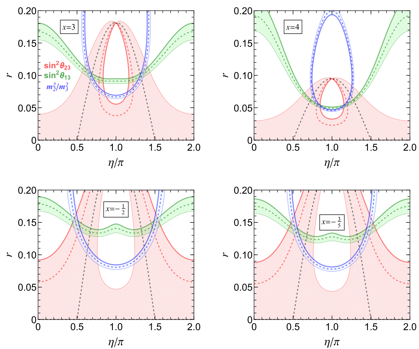
The original Littlest Seesaw model [18, 19, 20, 21] corresponds to the cases of $(x,\eta)=(3,2\pi/3)$, $(-1,-2\pi/3)$, and the CSD(4) model [22, 23] can be exactly reproduced for $(x,\eta)=(4,4\pi/5)$. From table 1, we see that the values $(x,\eta)=(-1/2,\pm\pi/2)$, $(-3/4,\pm 3\pi/5)$ and $(-4/5,\pm 3\pi/5)$ can give rise to a smaller $\chi^{2}_{\text{min}}$ than the original Littlest Seesaw model and CSD(4) model [18, 19, 20, 21, 22, 23]. We have shown $\chi^{2}_{\text{min}}$ as a function of $\eta$ for $x=3,4,-1/2,-3/4,-3/5$ in figure 1. Moreover, we plot the contour regions for the $3\sigma$ intervals of mixing angles $\theta_{13}$ and $\theta_{23}$ and mass ratio $m_{2}/m_{3}$ in the plane $r$ versus $\eta/\pi$ in figure 2. The result for $\theta_{12}$ is not displayed here, because it is related to the reactor angle $\theta_{13}$ by the TM1 mixing sum rule $\cos^{2}\theta_{12}\cos^{2}\theta_{13}=2/3$ which leads to $0.316\leq\sin^{2}\theta_{12}\leq 0.319$ for the $3\sigma$ allowed range of $\theta_{13}$ [8].

From figures 1 and 2, we notice that the values of $\chi^{2}_{\text{min}}$ is quite sensitive to the phase $\eta$ and predictions for the mixing angles and neutrino masses can agree very well with the experimental data for certain choices of $\eta$. Henceforth we shall focus on the new Littlest Seesaw model defined by the simple values $x=-1/2$ and $\eta=\pm\pi/2$ which give a phenomenologically successful and predictive description of lepton mixing parameters and neutrino masses, as highlighted with cyan background in table 1. Moreover, the corresponding vacuum alignment $\langle\phi_{\text{sol}}\rangle\propto\left(1,-1/2,5/2\right)$ and the phase $\eta=\pm\pi/2$ should be easy to realize in a concrete model. This new Littlest Seesaw model and the original Littlest Seesaw model differ in their predictions for $\theta_{23}$ and $\delta_{CP}$. The atmospheric mixing angle $\theta_{23}$ deviates from maximal mixing in the new Littlest Seesaw model while it is close to $45^{\circ}$ in the original Littlest Seesaw. Since deviation of $\theta_{23}$ from maximal mixing is preferred by the present data [8], the new littlest tri-direct CP model provides a better fit to the data of $\theta_{23}$ than the original Littlest Seesaw.

It is well-known fact that there is a predominance of matter over antimatter present in the observable Universe. The value of baryon asymmetry of the Universe normalised to the entropy density is [63],

Apart from elegantly explaining the tiny neutrino masses, the seesaw mechanism provides a simple and attractive mechanism for understanding the matter-antimatter asymmetry of the Universe via leptogenesis [64]. The out-of-equilibrium decays of right-handed neutrinos in the early Universe generates a lepton asymmetry because of the CP violating Yukawa couplings. The lepton asymmetry is subsequently converted into a baryon asymmetry via sphaleron processes in the SM.

In our concerned model, the phase $\eta$ is the unique source of CP violation, and it controls CP violation in both neutrino oscillations and leptogenesis. Therefore the measurable CP violation in future neutrino oscillation experiments are closely related to the baryon asymmetry of the Universe. In the present work, we shall focus on the simplest version of the leptogenesis in which the lepton asymmetry is dominantly generated by the interactions and decay of the lightest right-handed neutrino. The phase $\eta$ is fixed to $\eta=-\pi/2$ in the new Littlest Seesaw model, and it yields a Dirac CP violation phase $\delta_{CP}\simeq 1.646\pi$. In this section, we shall study the prediction for leptogenesis within the framework of SM and MSSM. The condition of successful baryogenesis will allow us to determine the mass of the lightest right-handed neutrino in the new Littlest Seesaw model.

References

- [1] S. F. King and C. Luhn, “Neutrino Mass and Mixing with Discrete Symmetry,” Rept. Prog. Phys. 76 (2013) 056201, arXiv:1301.1340 [hep-ph].
- [2] S. F. King, “Models of Neutrino Mass, Mixing and CP Violation,” J. Phys. G42 (2015) 123001, arXiv:1510.02091 [hep-ph].
- [3] P. Minkowski, “ at a Rate of One Out of Muon Decays?,” Phys. Lett. 67B (1977) 421–428.
- [4] R. N. Mohapatra and G. Senjanovic, “Neutrino Mass and Spontaneous Parity Nonconservation,” Phys. Rev. Lett. 44 (1980) 912. [,231(1979)].
- [5] J. Schechter and J. W. F. Valle, “Neutrino Masses in SU(2) x U(1) Theories,” Phys. Rev. D22 (1980) 2227.
- [6] S. F. King, “Atmospheric and solar neutrinos with a heavy singlet,” Phys. Lett. B439 (1998) 350–356, arXiv:hep-ph/9806440 [hep-ph].
- [7] S. F. King, “Atmospheric and solar neutrinos from single right-handed neutrino dominance and U(1) family symmetry,” Nucl. Phys. B562 (1999) 57–77, arXiv:hep-ph/9904210 [hep-ph].
- [8] I. Esteban, M. C. Gonzalez-Garcia, A. Hernandez-Cabezudo, M. Maltoni, and T. Schwetz, “Global analysis of three-flavour neutrino oscillations: synergies and tensions in the determination of , and the mass ordering,” JHEP 01 (2019) 106, arXiv:1811.05487 [hep-ph].
- [9] S. F. King, “Large mixing angle MSW and atmospheric neutrinos from single right-handed neutrino dominance and U(1) family symmetry,” Nucl. Phys. B576 (2000) 85–105, arXiv:hep-ph/9912492 [hep-ph].
- [10] P. H. Frampton, S. L. Glashow, and T. Yanagida, “Cosmological sign of neutrino CP violation,” Phys. Lett. B548 (2002) 119–121, arXiv:hep-ph/0208157 [hep-ph].
- [11] S. F. King, “Constructing the large mixing angle MNS matrix in seesaw models with right-handed neutrino dominance,” JHEP 09 (2002) 011, arXiv:hep-ph/0204360 [hep-ph].
- [12] W.-l. Guo, Z.-z. Xing, and S. Zhou, “Neutrino Masses, Lepton Flavor Mixing and Leptogenesis in the Minimal Seesaw Model,” Int. J. Mod. Phys. E16 (2007) 1–50, arXiv:hep-ph/0612033 [hep-ph].
- [13] K. Harigaya, M. Ibe, and T. T. Yanagida, “Seesaw Mechanism with Occam’s Razor,” Phys. Rev. D86 (2012) 013002, arXiv:1205.2198 [hep-ph].
- [14] J. Zhang and S. Zhou, “A Further Study of the Frampton-Glashow-Yanagida Model for Neutrino Masses, Flavor Mixing and Baryon Number Asymmetry,” JHEP 09 (2015) 065, arXiv:1505.04858 [hep-ph].
- [15] S. F. King, “Predicting neutrino parameters from SO(3) family symmetry and quark-lepton unification,” JHEP 08 (2005) 105, arXiv:hep-ph/0506297 [hep-ph].
- [16] S. Antusch, S. F. King, C. Luhn, and M. Spinrath, “Trimaximal mixing with predicted from a new type of constrained sequential dominance,” Nucl. Phys. B856 (2012) 328–341, arXiv:1108.4278 [hep-ph].
- [17] S. F. King, “Minimal predictive see-saw model with normal neutrino mass hierarchy,” JHEP 07 (2013) 137, arXiv:1304.6264 [hep-ph].
- [18] S. F. King, “Littlest Seesaw,” JHEP 02 (2016) 085, arXiv:1512.07531 [hep-ph].
- [19] S. F. King and C. Luhn, “Littlest Seesaw model from S U(1),” JHEP 09 (2016) 023, arXiv:1607.05276 [hep-ph].
- [20] P. Ballett, S. F. King, S. Pascoli, N. W. Prouse, and T. Wang, “Precision neutrino experiments vs the Littlest Seesaw,” JHEP 03 (2017) 110, arXiv:1612.01999 [hep-ph].
- [21] S. F. King, S. Molina Sedgwick, and S. J. Rowley, “Fitting high-energy Littlest Seesaw parameters using low-energy neutrino data and leptogenesis,” JHEP 10 (2018) 184, arXiv:1808.01005 [hep-ph].
- [22] S. F. King, “Minimal see-saw model predicting best fit lepton mixing angles,” Phys. Lett. B724 (2013) 92–98, arXiv:1305.4846 [hep-ph].
- [23] S. F. King, “A model of quark and lepton mixing,” JHEP 01 (2014) 119, arXiv:1311.3295 [hep-ph].
- [24] F. Bjrkeroth and S. F. King, “Testing constrained sequential dominance models of neutrinos,” J. Phys. G42 no. 12, (2015) 125002, arXiv:1412.6996 [hep-ph].
- [25] F. Feruglio, C. Hagedorn, and R. Ziegler, “Lepton Mixing Parameters from Discrete and CP Symmetries,” JHEP 07 (2013) 027, arXiv:1211.5560 [hep-ph].
- [26] M. Holthausen, M. Lindner, and M. A. Schmidt, “CP and Discrete Flavour Symmetries,” JHEP 04 (2013) 122, arXiv:1211.6953 [hep-ph].
- [27] G.-J. Ding, S. F. King, C. Luhn, and A. J. Stuart, “Spontaneous CP violation from vacuum alignment in models of leptons,” JHEP 05 (2013) 084, arXiv:1303.6180 [hep-ph].
- [28] G.-J. Ding, S. F. King, and A. J. Stuart, “Generalised CP and Family Symmetry,” JHEP 12 (2013) 006, arXiv:1307.4212 [hep-ph].
- [29] C.-C. Li and G.-J. Ding, “Generalised CP and trimaximal lepton mixing in family symmetry,” Nucl. Phys. B881 (2014) 206–232, arXiv:1312.4401 [hep-ph].
- [30] G.-J. Ding and Y.-L. Zhou, “Predicting lepton flavor mixing from (48) and generalized symmetries,” Chin. Phys. C39 no. 2, (2015) 021001, arXiv:1312.5222 [hep-ph].
- [31] G.-J. Ding and S. F. King, “Generalized and family symmetry,” Phys. Rev. D89 no. 9, (2014) 093020, arXiv:1403.5846 [hep-ph].
- [32] G.-J. Ding and Y.-L. Zhou, “Lepton mixing parameters from family symmetry and generalised CP,” JHEP 06 (2014) 023, arXiv:1404.0592 [hep-ph].
- [33] C.-C. Li and G.-J. Ding, “Deviation from bimaximal mixing and leptonic CP phases in S4 family symmetry and generalized CP,” JHEP 08 (2015) 017, arXiv:1408.0785 [hep-ph].
- [34] G.-J. Ding, S. F. King, and T. Neder, “Generalised CP and family symmetry in semi-direct models of leptons,” JHEP 12 (2014) 007, arXiv:1409.8005 [hep-ph].
- [35] P. Chen, C.-C. Li, and G.-J. Ding, “Lepton Flavor Mixing and CP Symmetry,” Phys. Rev. D91 (2015) 033003, arXiv:1412.8352 [hep-ph].
- [36] L. L. Everett, T. Garon, and A. J. Stuart, “A Bottom-Up Approach to Lepton Flavor and CP Symmetries,” JHEP 04 (2015) 069, arXiv:1501.04336 [hep-ph].
- [37] G. C. Branco, I. de Medeiros Varzielas, and S. F. King, “Invariant approach to CP in family symmetry models,” Phys. Rev. D92 no. 3, (2015) 036007, arXiv:1502.03105 [hep-ph].
- [38] C.-C. Li and G.-J. Ding, “Lepton Mixing in Family Symmetry and Generalized CP,” JHEP 05 (2015) 100, arXiv:1503.03711 [hep-ph].
- [39] A. Di Iura, C. Hagedorn, and D. Meloni, “Lepton mixing from the interplay of the alternating group A5 and CP,” JHEP 08 (2015) 037, arXiv:1503.04140 [hep-ph].
- [40] P. Ballett, S. Pascoli, and J. Turner, “Mixing angle and phase correlations from A5 with generalized CP and their prospects for discovery,” Phys. Rev. D92 no. 9, (2015) 093008, arXiv:1503.07543 [hep-ph].
- [41] G. C. Branco, I. de Medeiros Varzielas, and S. F. King, “Invariant approach to in unbroken ,” Nucl. Phys. B899 (2015) 14–36, arXiv:1505.06165 [hep-ph].
- [42] P. Chen, C.-Y. Yao, and G.-J. Ding, “Neutrino Mixing from CP Symmetry,” Phys. Rev. D92 no. 7, (2015) 073002, arXiv:1507.03419 [hep-ph].
- [43] G.-J. Ding and S. F. King, “Generalized CP and Family Symmetry for Semi-Direct Predictions of the PMNS Matrix,” Phys. Rev. D93 (2016) 025013, arXiv:1510.03188 [hep-ph].
- [44] P. Chen, G.-J. Ding, F. Gonzalez-Canales, and J. W. F. Valle, “Generalized reflection symmetry and leptonic CP violation,” Phys. Lett. B753 (2016) 644–652, arXiv:1512.01551 [hep-ph].
- [45] C.-C. Li, C.-Y. Yao, and G.-J. Ding, “Lepton Mixing Predictions from Infinite Group Series with Generalized CP,” JHEP 05 (2016) 007, arXiv:1601.06393 [hep-ph].
- [46] P. Chen, G.-J. Ding, and S. F. King, “Leptogenesis and residual CP symmetry,” JHEP 03 (2016) 206, arXiv:1602.03873 [hep-ph].
- [47] C.-Y. Yao and G.-J. Ding, “CP Symmetry and Lepton Mixing from a Scan of Finite Discrete Groups,” Phys. Rev. D94 no. 7, (2016) 073006, arXiv:1606.05610 [hep-ph].
- [48] C.-C. Li, J.-N. Lu, and G.-J. Ding, “ and CP symmetry and a model with maximal CP violation,” Nucl. Phys. B913 (2016) 110–131, arXiv:1608.01860 [hep-ph].
- [49] J.-N. Lu and G.-J. Ding, “Alternative Schemes of Predicting Lepton Mixing Parameters from Discrete Flavor and CP Symmetry,” Phys. Rev. D95 no. 1, (2017) 015012, arXiv:1610.05682 [hep-ph].
- [50] L. L. Everett and A. J. Stuart, “Lepton Sector Phases and Their Roles in Flavor and Generalized CP Symmetries,” Phys. Rev. D96 no. 3, (2017) 035030, arXiv:1611.03020 [hep-ph].
- [51] C.-C. Li and G.-J. Ding, “Implications of residual CP symmetry for leptogenesis in a model with two right-handed neutrinos,” Phys. Rev. D96 no. 7, (2017) 075005, arXiv:1701.08508 [hep-ph].
- [52] C.-C. Li, J.-N. Lu, and G.-J. Ding, “Toward a unified interpretation of quark and lepton mixing from flavor and CP symmetries,” JHEP 02 (2018) 038, arXiv:1706.04576 [hep-ph].
- [53] J.-N. Lu and G.-J. Ding, “Quark and lepton mixing patterns from a common discrete flavor symmetry with a generalized CP symmetry,” Phys. Rev. D98 no. 5, (2018) 055011, arXiv:1806.02301 [hep-ph].
- [54] J.-N. Lu and G.-J. Ding, “Dihedral flavor group as the key to understand quark and lepton flavor mixing,” JHEP 03 (2019) 056, arXiv:1901.07414 [hep-ph].
- [55] P. Chen, S. Centelles Chuli¨¢, G.-J. Ding, R. Srivastava, and J. W. F. Valle, “Neutrino Predictions from Generalized CP Symmetries of Charged Leptons,” JHEP 07 (2018) 077, arXiv:1802.04275 [hep-ph].
- [56] C. Hagedorn and E. Molinaro, “Flavor and CP symmetries for leptogenesis and decay,” Nucl. Phys. B919 (2017) 404–469, arXiv:1602.04206 [hep-ph].
- [57] L. A. Delgadillo, L. L. Everett, R. Ramos, and A. J. Stuart, “Predictions for the Dirac CP-Violating Phase from Sum Rules,” Phys. Rev. D97 no. 9, (2018) 095001, arXiv:1801.06377 [hep-ph].
- [58] G.-J. Ding, S. F. King, and C.-C. Li, “Tri-Direct CP in the Littlest Seesaw Playground,” JHEP 12 (2018) 003, arXiv:1807.07538 [hep-ph].
- [59] G.-J. Ding, S. F. King, and C.-C. Li, “Lepton Mixing Predictions from in the Tri-Direct CP approach to Two Right-handed Neutrino Models,” arXiv:1811.12340 [hep-ph].
- [60] G.-J. Ding, S. F. King, and C.-C. Li, “Golden Littlest Seesaw,” Nucl. Phys. B925 (2017) 470–499, arXiv:1705.05307 [hep-ph].
- [61] C. Jarlskog, “Commutator of the Quark Mass Matrices in the Standard Electroweak Model and a Measure of Maximal CP Violation,” Phys. Rev. Lett. 55 (1985) 1039.
- [62] G. C. Branco, L. Lavoura, and M. N. Rebelo, “Majorana Neutrinos and CP Violation in the Leptonic Sector,” Phys. Lett. B180 (1986) 264–268.
- [63] Planck Collaboration, N. Aghanim et al., “Planck 2018 results. VI. Cosmological parameters,” arXiv:1807.06209 [astro-ph.CO].
- [64] M. Fukugita and T. Yanagida, “Baryogenesis Without Grand Unification,” Phys. Lett. B174 (1986) 45–47.
- [65] E. Nardi, Y. Nir, E. Roulet, and J. Racker, “The Importance of flavor in leptogenesis,” JHEP 01 (2006) 164, arXiv:hep-ph/0601084 [hep-ph].
- [66] A. Abada, S. Davidson, A. Ibarra, F. X. Josse-Michaux, M. Losada, and A. Riotto, “Flavour Matters in Leptogenesis,” JHEP 09 (2006) 010, arXiv:hep-ph/0605281 [hep-ph].
- [67] A. Abada, S. Davidson, F.-X. Josse-Michaux, M. Losada, and A. Riotto, “Flavor issues in leptogenesis,” JCAP 0604 (2006) 004, arXiv:hep-ph/0601083 [hep-ph].
- [68] S. Antusch, S. F. King, and A. Riotto, “Flavour-Dependent Leptogenesis with Sequential Dominance,” JCAP 0611 (2006) 011, arXiv:hep-ph/0609038 [hep-ph].
- [69] G. F. Giudice, A. Notari, M. Raidal, A. Riotto, and A. Strumia, “Towards a complete theory of thermal leptogenesis in the SM and MSSM,” Nucl. Phys. B685 (2004) 89–149, arXiv:hep-ph/0310123 [hep-ph].
- [70] W. Buchmuller, P. Di Bari, and M. Plumacher, “Leptogenesis for pedestrians,” Annals Phys. 315 (2005) 305–351, arXiv:hep-ph/0401240 [hep-ph].
- [71] L. Covi, E. Roulet, and F. Vissani, “CP violating decays in leptogenesis scenarios,” Phys. Lett. B384 (1996) 169–174, arXiv:hep-ph/9605319 [hep-ph].
- [72] W. Buchmuller, R. D. Peccei, and T. Yanagida, “Leptogenesis as the origin of matter,” Ann. Rev. Nucl. Part. Sci. 55 (2005) 311–355, arXiv:hep-ph/0502169 [hep-ph].
- [73] S. Davidson, E. Nardi, and Y. Nir, “Leptogenesis,” Phys. Rept. 466 (2008) 105–177, arXiv:0802.2962 [hep-ph].
- [74] J. A. Harvey and M. S. Turner, “Cosmological baryon and lepton number in the presence of electroweak fermion number violation,” Phys. Rev. D42 (1990) 3344–3349.
- [75] G. Altarelli and F. Feruglio, “Tri-bimaximal neutrino mixing, A(4) and the modular symmetry,” Nucl. Phys. B741 (2006) 215–235, arXiv:hep-ph/0512103 [hep-ph].
- [76] F. Feruglio, “Are neutrino masses modular forms?,” in From My Vast Repertoire …: Guido Altarelli’s Legacy, A. Levy, S. Forte, and G. Ridolfi, eds., pp. 227–266. 2019. arXiv:1706.08749 [hep-ph].
- [77] G.-J. Ding, S. F. King, X.-G. Liu, and J.-N. Lu, “Modular S4 and A4 symmetries and their fixed points: new predictive examples of lepton mixing,” JHEP 12 (2019) 030, arXiv:1910.03460 [hep-ph].
- [78] F. Borzumati and A. Masiero, “Large Muon and electron Number Violations in Supergravity Theories,” Phys. Rev. Lett. 57 (1986) 961.
- [79] J. Hisano, T. Moroi, K. Tobe, and M. Yamaguchi, “Lepton flavor violation via right-handed neutrino Yukawa couplings in supersymmetric standard model,” Phys. Rev. D53 (1996) 2442–2459, arXiv:hep-ph/9510309 [hep-ph].
- [80] Particle Data Group Collaboration, M. Tanabashi et al., “Review of Particle Physics,” Phys. Rev. D98 no. 3, (2018) 030001.