跳到论文正文
W Papers独立论文阅读器 arXiv:1906.11364 论文正文 计算阅读时间 · 0%
引用这篇论文根据当前论文元数据生成,正式投稿前建议核对。


License: arXiv.org perpetual non-exclusive license
arXiv:1906.11364v3 [math.ST] 09 Oct 2021

Daren Wang, Zifeng Zhao, Kevin Z. Lin and Rebecca Willett

Statistically and Computationally Efficient Change Point Localization in Regression Settings

Daren Wang dwang24@nd.edu Affiliation: Department of ACMS Affiliation: University of Notre Dame Affiliation: Indiana, USA    Zifeng Zhao zifeng.zhao@nd.edu Affiliation: Mendoza College of Business Affiliation: University of Notre Dame Affiliation: Indiana, USA    Kevin Z. Lin kevinl1@wharton.upenn.edu Affiliation: Department of Statistics and Data Science Affiliation: University of Pennsylvania Affiliation: Pennsylvania, USA    Rebecca Willett willett@uchicago.edu Affiliation: Department of Statistics Affiliation: University of Chicago Affiliation: Illinois, USA
Abstract

Detecting when the underlying distribution changes for the observed time series is a fundamental problem arising in a broad spectrum of applications. In this paper, we study multiple change-point localization in the high-dimensional regression setting, which is particularly challenging as no direct observations of the parameter of interest is available. Specifically, we assume we observe {xt,yt}t=1n\{x_{t},y_{t}\}_{t=1}^{n} where {xt}t=1n\{x_{t}\}_{t=1}^{n} are pp-dimensional covariates, {yt}t=1n\{y_{t}\}_{t=1}^{n} are the univariate responses satisfying 𝔼⁡(yt)=xt⊤​βt∗​ for ​1≤t≤n\mathbb{E}(y_{t})=x_{t}^{\top}\beta_{t}^{*}\text{ for }1\leq t\leq n and {βt∗}t=1n\{\beta_{t}^{*}\}_{t=1}^{n} are the unobserved regression coefficients that change over time in a piecewise constant manner. We propose a novel projection-based algorithm, Variance Projected Wild Binary Segmentation (VPWBS), which transforms the original (difficult) problem of change-point detection in pp-dimensional regression to a simpler problem of change-point detection in mean of a one-dimensional time series. VPWBS is shown to achieve sharp localization rate Op​(1/n)O_{p}(1/n) up to a log factor, a significant improvement from the best rate Op​(1/n)O_{p}(1/\sqrt{n}) known in the existing literature for multiple change-point localization in high-dimensional regression. Extensive numerical experiments are conducted to demonstrate the robust and favorable performance of VPWBS over two state-of-the-art algorithms, especially when the size of change in the regression coefficients {βt∗}t=1n\{\beta_{t}^{*}\}_{t=1}^{n} is small.

††heading: 22 2021 1- 6/19; Revised 7/21 10/21 19-531††shortheadings: Regression Change Point Detection in High-dimension / Wang, Zhao, Lin, Willett††firstpage: 1††editor: Zaid Harchaoui


keywords
Change-point detection; High-dimensional regression; CUSUM statistics; Wild binary segmentation; Time series analysis

1 Introduction

Change-point detection and localization is a classical problem in time series analysis, in which we record a series of measurements and wish to determine whether and at what time(s) the underlying generative model has changed. Due to its flexibility, the model of a time series with multiple structural changes has a wide range of applications including econometrics [Bai and Perron 1998], epidemiology [Jiang et al. 2021], stock price analysis [Chen and Gupta 1997], Internet security monitoring [Peng et al. 2004], and genetics [Castro et al. 2018; Zhao and Yau 2021].

Change-point detection is mostly studied and well understood in the mean change-point model, where we typically assume we observe a time series {yt}t=1n⊂ℝp\{y_{t}\}_{t=1}^{n}\subset\mathbb{R}^{p} such that

yt=βt∗+εt, for all ​1≤t≤n.y_{t}=\beta_{t}^{*}+\varepsilon_{t},\text{ for all }1\leq t\leq n.

Here {εt}t=1n\{\varepsilon_{t}\}_{t=1}^{n} are independently and identically distributed measurement noise with mean zero and {βt∗}t=1n\{\beta_{t}^{*}\}_{t=1}^{n} are the population mean vectors that change over time in a piecewise constant manner. The important task is to determine whether and where the structural changes of {βt∗}t=1n\{\beta_{t}^{*}\}_{t=1}^{n} take place. There is a vast literature of change-point detection in mean for both low and high dimensions, see for example Frick et al. 2014, Cho and Fryzlewicz 2015, Cho et al. 2016, Yau and Zhao 2016 and Wang and Samworth 2018. More recently, Pein et al. 2017 introduced a method that can handle mean and variance changes simultaneously. Cribben and Yu 2017, Wang et al. 2021 and Zhao et al. 2019, among others, investigated the mean change-point problem for the dynamic Bernoulli network models. Enikeeva and Harchaoui 2019 studied the optimal change point detection boundary in the high-dimensional settings. Xie et al. 2020 considered online monitoring change point detection for streaming data in high dimensions.

However, in some other practical settings , we can only obtain indirect measurements of the (potentially high-dimensional) vectors {βt∗}t=1n\{\beta_{t}^{*}\}_{t=1}^{n}. Specifically, in this paper, we consider change-point detection in high-dimensional linear regression. We assume we observe the time series {xt,yt}t=1n\{x_{t},y_{t}\}_{t=1}^{n}, where {xt}t=1n\{x_{t}\}_{t=1}^{n} are pp-dimensional covariates, {yt}t=1n\{y_{t}\}_{t=1}^{n} are the univariate responses satisfying 𝔼⁡(yt|xt)=xt⊤​βt∗​ for all ​1≤t≤n\mathbb{E}(y_{t}|x_{t})=x_{t}^{\top}\beta_{t}^{*}\text{ for all }1\leq t\leq n and {βt∗}t=1n\{\beta_{t}^{*}\}_{t=1}^{n} are the unobserved regression coefficients that potentially change over time. We formally summarize the model as follows.

Model 1 (Change-point model in the regression setting).

Suppose for 1≤t≤n1\leq t\leq n, the random covariate xt∈ℝpx_{t}\in\mathbb{R}^{p} and response yt∈ℝy_{t}\in\mathbb{R} satisfy

yt=xt⊤​βt∗+εt,\displaystyle y_{t}=x_{t}^{\top}\beta_{t}^{*}+\varepsilon_{t}, (1)

where the noise εt​∼i.i.d.​𝒩​(0,σε2)\varepsilon_{t}\overset{i.i.d.}{\sim}\mathcal{N}(0,\sigma_{\varepsilon}^{2}) and is independent of the covariate xt​∼i.i.d.​𝒩​(0,Σ)x_{t}\overset{i.i.d.}{\sim}\mathcal{N}(0,\Sigma)11 1 We assume for convenience that εt\varepsilon_{t} and xtx_{t} are normally distributed. However our results remain valid as long as εt\varepsilon_{t} and xtx_{t} are i.i.d. sub-Gaussian random variables.. In addition, there exist K≥0K\geq 0 change-points {ηk}k=1K⊂{1,…,n−1}\{\eta_{k}\}_{k=1}^{K}\subset\{1,\ldots,n-1\} such that

βt∗=βt′∗ if ηk−1+1≤t≤t′≤ηk, for all k=1,⋯,K+1,\beta_{t}^{*}=\beta_{t^{\prime}}^{*}\text{\hskip 10.22217ptif \ }\eta_{k-1}+1\leq t\leq t^{\prime}\leq\eta_{k},\text{\hskip 10.22217ptfor all \ }k=1,\cdots,K+1,

where by convention we define η0=0\eta_{0}=0 and ηK+1=n\eta_{K+1}=n.

Notation: Before we proceed, for clarity of presentation, we first introduce necessary notation used throughout the paper. For two positive sequences {an}n=1∞\{a_{n}\}_{n=1}^{\infty} and {bn}n=1∞\{b_{n}\}_{n=1}^{\infty}, we write an=O⁡(bn)a_{n}=O(b_{n}) if there exists C>0C>0 such that limsupn→∞an/bn<C\lim\sup_{n\to\infty}a_{n}/b_{n}<C and write an≍bna_{n}\asymp b_{n} or an=Θ⁡(bn)a_{n}=\Theta(b_{n}) if an=O⁡(bn)a_{n}=O(b_{n}) and bn=O⁡(an)b_{n}=O(a_{n}). We write an⪰bna_{n}\succeq b_{n} if liminfn→∞an/bn=∞.\lim\inf_{n\to\infty}a_{n}/b_{n}=\infty. Let {xn}n=1∞\{x_{n}\}_{n=1}^{\infty} be a sequence of random variables. We write xn=Op​(bn)x_{n}=O_{p}(b_{n}) if xn/bn=Op​(1)x_{n}/b_{n}=O_{p}(1) and write xn=op​(bn)x_{n}=o_{p}(b_{n}) if xn/bn=op​(1)x_{n}/b_{n}=o_{p}(1), where Op​(1)O_{p}(1) and op​(1)o_{p}(1) follow the standard probability notation of big OO (stochastic boundedness) and small oo (convergence to zero in probability). For a vector β∈ℝp\beta\in\mathbb{R}^{p}, denote ‖β‖2=∑i=1pβi2\|\beta\|_{2}=\sqrt{\sum_{i=1}^{p}{\beta_{i}^{2}}} as its l2l_{2} norm, denote ‖β‖∞=max1≤i≤p⁡|βi|\|\beta\|_{\infty}=\max_{1\leq i\leq p}|\beta_{i}| as its l∞l_{\infty} norm, and denote ‖β‖0=∑i=1p𝕀⁡(βi≠0)\|\beta\|_{0}=\sum_{i=1}^{p}\mathbb{I}(\beta_{i}\neq 0) as its l0l_{0} norm, where βi\beta_{i} denotes the iith element of β\beta and 𝕀\mathbb{I} is the indicator function. Given two natural numbers s<es<e, for simplicity, with a slight abuse of notation, we denote [s,e]:={t∈ℕ|s≤t≤e}[s,e]:=\{t\in\mathbb{N}|s\leq t\leq e\} and denote (s,e]:={t∈ℕ|s<t≤e}(s,e]:=\{t\in\mathbb{N}|s<t\leq e\}. In other words, [s,e][s,e] contains all natural numbers from ss to ee (inclusive) and (s,e](s,e] contains all natural numbers from s+1s+1 to ee (inclusive). Throughout the paper, we use cc and CC to denote generic absolute constants independent of nn and pp, and the value of cc and CC may vary from place to place.

For change-point detection in Model (1), the key task is to estimate the unknown {ηk}k=1K\{\eta_{k}\}_{k=1}^{K}. For any change-point estimator {η^k}k=1K′\{\widehat{\eta}_{k}\}_{k=1}^{K^{\prime}}, we say it is consistent if, with probability approaching 1, K′=KK^{\prime}=K and the sup-norm error satisfies

ϵ:=max1≤k≤K⁡|η^k−ηk|n=op​(1).\displaystyle\epsilon:=\max_{1\leq k\leq K}\frac{|\widehat{\eta}_{k}-\eta_{k}|}{n}=o_{p}(1). (2)

for all sufficiently large nn.

In the literature, change-point detection for low-dimensional (p≪n)(p\ll n) linear regression models has been extensively studied by many authors including Bai and Perron 1998, Qu and Perron 2007, and more recently Zhang et al. 2015b. Most of the existing works in this setting focus on the case where the number of change-points, KK, is a fixed constant.

Change-point detection for the high-dimensional linear regression model where p≫np\gg n, has also received recent attention. In particular, Lee et al. 2016 extended Lasso to the high-dimensional single change-point setting and showed that both the change-point and the regression parameters {βt∗}t=1n\{\beta_{t}^{*}\}_{t=1}^{n} can be consistently estimated. Later, Lee et al. 2018 extended their results to the high-dimensional quantile regression model. Kaul et al. 2019 proposed a highly efficient algorithm for the setting of exactly one change-point. Both Lee et al. 2016 and Kaul et al. 2019 showed that in the single change-point setting, the change-point can be estimated with sup-norm error satisfying ϵ=Op​(1/n)\epsilon=O_{p}(1/n). Zhang et al. 2015a studied the Sparse Group Lasso (SGL) algorithm for the multiple change-points setting. The authors showed that SGL returns consistent change-point estimators with ϵ=op​(1)\epsilon=o_{p}(1) when the number of change-points KK is bounded. Leonardi and Bühlmann 2016 showed that, by using a binary search algorithm, consistent estimation can be achieved with ϵ=Op​(1/n)\epsilon=O_{p}(1/\sqrt{n}) even when the number of change-points KK diverges as n→∞n\to\infty.

In this paper, we focus on the high-dimensional regime (p≫np\gg n) and propose a computationally efficient algorithm that can consistently estimate the unknown multiple change-points at the minimax optimal localization rate Op​(1/n)O_{p}(1/n) up to a log factor. To the best of our knowledge, no other method in the literature can achieve this rate for multiple change-points estimation under such setting. We refer to more detailed discussion of our contribution at the end of this section.

We proceed by imposing some mild general assumptions on the high-dimensional regression setting in Model (1) and define key quantities that are used to quantify the localization error rate and requirements on the signal-to-noise ratio (SNR) of various change-point estimation methods for Model (1).

{assumption}


a. [Design matrix] There exist absolute positive constants cxc_{x} and CxC_{x} such that the minimal and maximal eigenvalues of the covariance matrix Σ\Sigma satisfy Λmin​(Σ)≥cx\Lambda_{\min}(\Sigma)\geq c_{x} and Λmax​(Σ)≤Cx\Lambda_{\max}(\Sigma)\leq C_{x}.
b. [Sparse support] There exist a collection of subsets {Sk}k=1K+1⊂ℝp\{S_{k}\}_{k=1}^{K+1}\subset\mathbb{R}^{p} such that, for all k=1,⋯,K+1k=1,\cdots,K+1,

βt,j∗=0​ if ​ηk−1+1≤t≤ηk+1​ and ​j∉Sk.\beta^{*}_{t,j}=0\text{ if }\eta_{k-1}+1\leq t\leq\eta_{k+1}\text{ and }j\not\in S_{k}.

In addition, the size of the support satisfies max1≤k≤K+1⁡|Sk|≤𝔰\max_{1\leq k\leq K+1}|S_{k}|\leq\mathfrak{s} and there exists an absolute constant CβC_{\beta} such that max1≤t≤n⁡‖βt∗‖∞≤Cβ<∞.\max_{1\leq t\leq n}\|\beta_{t}^{*}\|_{\infty}\leq C_{\beta}<\infty.

Key quantities: Define 𝔑:=max1≤t≤n⁡‖βt∗‖22\mathfrak{N}:=\max_{1\leq t\leq n}\|\beta_{t}^{*}\|_{2}^{2}. By Assumption 1b, we have 𝔑≤Cβ2​𝔰\mathfrak{N}\leq C_{\beta}^{2}{\mathfrak{s}}. Moreover, by Assumption 1a, we have Var​(yt)=βt∗⁣⊤​Σ​βt∗+σε2>cx​‖βt∗‖22\text{Var}(y_{t})=\beta_{t}^{*\top}\Sigma\beta_{t}^{*}+\sigma_{\varepsilon}^{2}>c_{x}\|\beta_{t}^{*}\|_{2}^{2}, and thus 𝔑<max1≤t≤n⁡Var​(yt)/cx{\mathfrak{N}}<\max_{1\leq t\leq n}\text{Var}(y_{t})/c_{x}. For k=1,⋯,K+1k=1,\cdots,K+1, denote Δk=ηk−ηk−1\Delta_{k}=\eta_{k}-\eta_{k-1} as the spacing between two consecutive change-points and define Δ=min1≤k≤K+1⁡Δk\Delta=\min_{1\leq k\leq K+1}\Delta_{k} as the minimum spacing. In addition, for k=1,⋯Kk=1,\cdots K, denote κk=‖βηk+1∗−βηk∗‖2\kappa_{k}=\left\|\beta^{*}_{\eta_{k}+1}-\beta_{\eta_{k}}^{*}\right\|_{2} as the l2l_{2}-norm of the change in regression coefficients and define κ=min1≤k≤K⁡κk\kappa=\min_{1\leq k\leq K}\kappa_{k} as the minimum change size. Intuitively, the difficulty of change-point detection for Model 1 depends on the interplay among KK, κ\kappa, Δ\Delta, 𝔰\mathfrak{s}, the dimension pp and the sample size nn.

We remark that our later theoretical analysis allows the number of change-points KK, the minimum change size κ\kappa, the minimum spacing Δ\Delta, the sparsity 𝔰\mathfrak{s} and the dimension pp to vary with the sample size nn. To our best knowledge, this is among the most flexible frameworks in the literature.

Our contributions: For change-point estimation in the high-dimensional regression model, we propose a novel two-stage detection procedure named Variance Projected Wild Binary Segmentation (VPWBS). Given the observations {xt,yt}t=1n\{x_{t},y_{t}\}_{t=1}^{n}, in Stage 1, VPWBS estimates the regression coefficients {βt∗}t=1n\{\beta_{t}^{*}\}_{t=1}^{n} using a group Lasso based local screening algorithm carefully tailored for the high-dimensional regression change-point setting. In Stage 2, via a novel projection step, VPWBS projects the high-dimensional regression data {xt,yt}t=1n\{x_{t},y_{t}\}_{t=1}^{n} into a one-dimensional time series, where the optimal projection direction is derived from the estimated {β^t}t=1n\{\widehat{\beta}_{t}\}_{t=1}^{n} in Stage 1. Subsequently, VPWBS achieves change-point estimation by performing mean change detection via CUSUM statistics on the resulting one-dimensional time series.

Our theoretical analysis shows that VPWBS can achieve consistent estimation even when the number of change-points KK diverges as n→∞n\to\infty. Furthermore, the sup-norm error ϵ\epsilon (defined in (2)) of the VPWBS change-point estimator is, up to a log factor, of order Op​(1/n)O_{p}(1/n), which is the known minimax optimal rate. To the best of our knowledge, this is a significant improvement for multiple change-point estimation in the high-dimensional regression setting, as the aforementioned existing literature can only achieve ϵ=Op​(1/n)\epsilon=O_{p}(1/\sqrt{n}) at best. A key step of VPWBS is the estimation of an optimal projection direction. In the theoretical analysis, we establish error bounds on the estimated high-dimensional projection direction, which may be of independent interest. VPWBS admits a reasonable computational cost of order O⁡(n​(log⁡(n))2⋅GroupLasso​(n,p))O(n(\log(n))^{2}\cdot\text{GroupLasso}(n,p)), which enables its implementation in the high-dimensional regression setting. Here GroupLasso​(n,p)\text{GroupLasso}(n,p) denotes the computational cost of the group Lasso for a pp-dimensional regression with nn samples. Similar definition applies to Lasso​(n,p)\text{Lasso}(n,p). We summarize the localization error bound and computational cost of VPWBS and two other state-of-the-art methods in Table 1 and refer more detailed discussions to Sections 3 and 4.

Localization Error Bound ϵ\epsilon SNR Condition Computational Complexity
VPWBS Op​(𝔑​log⁡(n)​n−1)O_{p}\big(\mathfrak{N}\log(n)n^{-1}\big) Δ​κ2⪰𝔰​log⁡(p​n)\Delta\kappa^{2}\succeq{\mathfrak{s}}\log(pn) O⁡(n​(log⁡(n))2⋅GroupLasso ​(n,p))O(n(\log(n))^{2}\cdot\text{GroupLasso }(n,p))
EBSA Op(𝔰log(p)n−1/2)O_{p}\big({\mathfrak{s}}\log(p)n^{-1/2}\big) Δ​κ2⪰𝔑​𝔰​log⁡(p)\Delta\kappa^{2}\succeq\mathfrak{N}{\mathfrak{s}}\log(p) O⁡(n​log⁡(n)⋅Lasso ​(n,p))O(n\log(n)\cdot\text{Lasso }(n,p))
SGL op​(1)o_{p}(1) Δ​κ2≍n\Delta\kappa^{2}\asymp n O​(Lasso​(n,n​p))O(\text{Lasso}(n,np))
Table 1: SGL (Zhang et al. 2015b) and EBSA (Leonardi and Bühlmann 2016) are two state-of-the-art methods developed for change-point estimation in high-dimensional regression. Recall 𝔑≤Cβ2​𝔰\mathfrak{N}\leq C_{\beta}^{2}{\mathfrak{s}} and we refer the detailed definition of notation n,p,Δ,κ,𝔰,𝔑n,p,\Delta,\kappa,{\mathfrak{s}},\mathfrak{N} to Assumption 1 and the discussion on key quantities.

The rest of the paper is organized as follows. In Section 2, we introduce the projection based change-point estimation framework and a group Lasso based local screening algorithm for the estimation of the optimal projection direction. Building upon wild binary segmentation, Section 3 proposes the VPWBS for multiple change-point estimation in high-dimensional regression and further establishes its optimal theoretical properties. Extensive numerical experiments are conducted in Section 4 to demonstrate the promising performance of VPWBS when compared with state-of-the-art methods in the literature. Section 5 concludes with a discussion. Technical proofs can be found in the supplementary material.

2 A General Framework and Group Lasso Based Screening

In this section, we introduce the general framework of the proposed change-point estimation procedure for the high-dimensional regression problem in Model (1). Specifically, Section 2.1 discusses the essential idea of a projection based change-point detection framework and Section 2.2 proposes a group Lasso based screening algorithm for estimating the unknown projection direction.

2.1 A projection based change-point estimation framework

To ease presentation, we start the discussion with the problem of single change-point estimation. Specifically, given a sample of high-dimensional regression {xt,yt}t=1n\{x_{t},y_{t}\}_{t=1}^{n} with yt=xt⊤​βt∗+εty_{t}=x_{t}^{\top}\beta_{t}^{*}+\varepsilon_{t}, assume there is a single change-point at an unknown time point η\eta such that

βt∗=β(1)​ for ​1≤t≤η​ and ​βt∗=β(2)​ for ​η+1≤t≤n.\beta_{t}^{*}=\beta^{(1)}\text{ for }1\leq t\leq\eta\text{ and }\beta_{t}^{*}=\beta^{(2)}\text{ for }\eta+1\leq t\leq n.

To detect the existence of η\eta and further estimate its location, we need to measure and test the difference between the unknown regression coefficients β(1)\beta^{(1)} and β(2)\beta^{(2)}.

For two regression coefficients β(1)\beta^{(1)} and β(2)\beta^{(2)}, it is natural to directly measure their difference via the l2l_{2}-norm ‖β(1)−β(2)‖22.\|\beta^{(1)}-\beta^{(2)}\|_{2}^{2}. However, under the regression context, an arguably more relevant alternative is (β(1)−β(2))⊤​Σ​(β(1)−β(2)){(\beta^{(1)}-\beta^{(2)})^{\top}\Sigma(\beta^{(1)}-\beta^{(2)})}, which equals to Var​(xt⊤​(β(1)−β(2))){\text{Var}(x_{t}^{\top}(\beta^{(1)}-\beta^{(2)}))} as Var​(xt)=Σ\text{Var}(x_{t})=\Sigma. Note that under Assumption 1a, we have that

cx​‖β(1)−β(2)‖22≤(β(1)−β(2))⊤​Σ​(β(1)−β(2))≤Cx​‖β(1)−β(2)‖22.c_{x}\|\beta^{(1)}-\beta^{(2)}\|_{2}^{2}\leq{(\beta^{(1)}-\beta^{(2)})^{\top}\Sigma(\beta^{(1)}-\beta^{(2)})}\leq C_{x}\|\beta^{(1)}-\beta^{(2)}\|_{2}^{2}.

Thus, in terms of theoretical magnitude, ‖β(1)−β(2)‖22\|\beta^{(1)}-\beta^{(2)}\|_{2}^{2} and (β(1)−β(2))⊤​Σ​(β(1)−β(2)){(\beta^{(1)}-\beta^{(2)})^{\top}\Sigma(\beta^{(1)}-\beta^{(2)})} are the same and both can capture the change in the regression coefficient. However, compared to ‖β(1)−β(2)‖22\|\beta^{(1)}-\beta^{(2)}\|_{2}^{2}, the quantity (β(1)−β(2))⊤​Σ​(β(1)−β(2)){(\beta^{(1)}-\beta^{(2)})^{\top}\Sigma(\beta^{(1)}-\beta^{(2)})} further incorporates the covariance structure Σ\Sigma of the covariates and thus can better reflect the difference between two regression models y=x⊤​β(1)+εy=x^{\top}\beta^{(1)}+\varepsilon and y=x⊤​β(2)+εy=x^{\top}\beta^{(2)}+\varepsilon. We therefore prefer (β(1)−β(2))⊤​Σ​(β(1)−β(2)){(\beta^{(1)}-\beta^{(2)})^{\top}\Sigma(\beta^{(1)}-\beta^{(2)})} for change-point estimation. We remark that (β(1)−β(2))⊤​Σ​(β(1)−β(2)){(\beta^{(1)}-\beta^{(2)})^{\top}\Sigma(\beta^{(1)}-\beta^{(2)})} is closely related to the explained variance in the regression literature, see for example Cai and Guo 2020.

For any 1≤m≤n−11\leq m\leq n-1, define βm(1)=∑t=1mβt∗/m\beta^{(1)}_{m}=\sum_{t=1}^{m}\beta_{t}^{*}/m and βm(2)=∑t=m+1nβt∗/(n−m)\beta^{(2)}_{m}=\sum_{t=m+1}^{n}\beta_{t}^{*}/(n-m). Note that βm(1)\beta^{(1)}_{m} and βm(2)\beta^{(2)}_{m} are the unique minimizer of the population squared loss function 𝔼⁡(∑t=1m(yt−xt⊤​β)2)\mathbb{E}(\sum_{t=1}^{m}(y_{t}-x_{t}^{\top}\beta)^{2}) and 𝔼⁡(∑t=m+1n(yt−xt⊤​β)2)\mathbb{E}(\sum_{t=m+1}^{n}(y_{t}-x_{t}^{\top}\beta)^{2}), respectively. As a function of mm, (βm(1)−βm(2))⊤​Σ​(βm(1)−βm(2)){(\beta_{m}^{(1)}-\beta_{m}^{(2)})^{\top}\Sigma(\beta_{m}^{(1)}-\beta_{m}^{(2)})} achieves its maximum at the true change-point m=ηm=\eta due to the fact that βm(1)−βm(2)=min⁡(ηm,n−ηn−m)​(β(1)−β(2))\beta_{m}^{(1)}-\beta_{m}^{(2)}=\min(\frac{\eta}{m},\frac{n-\eta}{n-m})(\beta^{(1)}-\beta^{(2)}). Thus, the sample estimate of (βm(1)−βm(2))⊤​Σ​(βm(1)−βm(2)){(\beta_{m}^{(1)}-\beta_{m}^{(2)})^{\top}\Sigma(\beta_{m}^{(1)}-\beta_{m}^{(2)})} can be valuable for the detection and estimation of η.\eta.

Given a time point mm, to estimate (βm(1)−βm(2))⊤​Σ​(βm(1)−βm(2)){(\beta_{m}^{(1)}-\beta_{m}^{(2)})^{\top}\Sigma(\beta_{m}^{(1)}-\beta_{m}^{(2)})}, a natural choice is the plug-in estimator. Specifically, via a penalized M-estimator, we can obtain β^m(1)\widehat{\beta}^{(1)}_{m} from {xt,yt}t=1m\{x_{t},y_{t}\}_{t=1}^{m} and β^m(2)\widehat{\beta}^{(2)}_{m} from {xt,yt}t=m+1n\{x_{t},y_{t}\}_{t=m+1}^{n}. Combined with a covariance matrix estimator Σ^\widehat{\Sigma}, the plug-in estimator takes the form (β^m(1)−β^m(2))⊤​Σ^​(β^m(1)−β^m(2))(\widehat{\beta}^{(1)}_{m}-\widehat{\beta}^{(2)}_{m})^{\top}\widehat{\Sigma}(\widehat{\beta}^{(1)}_{m}-\widehat{\beta}^{(2)}_{m}). This in some sense resembles the classical Wald-type statistics used in the change-point literature, see for example Richard A. Davis 1995 and Hušková et al. 2007. However, the plug-in estimator requires the estimation of Σ\Sigma. Without strong structural assumptions on Σ\Sigma, this is known to be a difficult task in high dimensions.

To bypass this difficulty, we slightly alter the estimation target and propose an alternative estimator via projection. Specifically, given a pp-dimensional unit vector uu with ‖u‖2=1\|u\|_{2}=1, we define the one-dimensional variance-projected time series {zt​(u)}t=1n\{z_{t}(u)\}_{t=1}^{n} as

zt(u)=u⊤xtyt, for t=1,⋯,n.z_{t}(u)=u^{\top}x_{t}y_{t},\text{ for }t=1,\cdots,n.

A key observation is that {zt​(u)}t=1n\{z_{t}(u)\}_{t=1}^{n} has a single change-point in mean at time point η\eta as long as u⊤​Σ​(β(1)−β(2))≠0u^{\top}\Sigma(\beta^{(1)}-\beta^{(2)})\neq 0. Importantly, if u=(β(1)−β(2))/‖β(1)−β(2)‖2u=(\beta^{(1)}-\beta^{(2)})/\|\beta^{(1)}-\beta^{(2)}\|_{2}, we have that

𝔼⁡(1m​∑t=1mzt​(u)−1n−m​∑t=m+1nzt​(u))=u⊤​Σ​(βm(1)−βm(2))\displaystyle\mathbb{E}\left(\frac{1}{m}\sum_{t=1}^{m}z_{t}(u)-\frac{1}{n-m}\sum_{t=m+1}^{n}z_{t}(u)\right)=u^{\top}\Sigma(\beta^{(1)}_{m}-\beta^{(2)}_{m})
=\displaystyle= min⁡(ηm,n−ηn−m)​(β(1)−β(2))⊤​Σ​(β(1)−β(2))‖β(1)−β(2)‖2,\displaystyle\min(\frac{\eta}{m},\frac{n-\eta}{n-m})\frac{(\beta^{(1)}-\beta^{(2)})^{\top}\Sigma(\beta^{(1)}-\beta^{(2)})}{\|\beta^{(1)}-\beta^{(2)}\|_{2}}, (3)

which is proportional to the key quantity (β(1)−β(2))⊤​Σ​(β(1)−β(2))(\beta^{(1)}-\beta^{(2)})^{\top}\Sigma(\beta^{(1)}-\beta^{(2)}) and also achieves its maximum at m=η.m=\eta. Note that we further have

(2.1)≥min⁡(ηm,n−ηn−m)​cx​‖β(1)−β(2)‖2.\eqref{eq:projection_mean}\geq\min(\frac{\eta}{m},\frac{n-\eta}{n-m})c_{x}\|\beta^{(1)}-\beta^{(2)}\|_{2}.

Thus, the projection direction u=(β(1)−β(2))/‖β(1)−β(2)‖2u=(\beta^{(1)}-\beta^{(2)})/\|\beta^{(1)}-\beta^{(2)}\|_{2} is optimal in the sense that it preserves the original change size ‖β(1)−β(2)‖2\|\beta^{(1)}-\beta^{(2)}\|_{2} of the regression coefficients. Therefore, if the projection direction uu is reasonably aligned with β(1)−β(2)\beta^{(1)}-\beta^{(2)}, we can efficiently detect and estimate the change-point η\eta by performing change-point estimation in mean on the univariate time series {zt​(u)}t=1n\{z_{t}(u)\}_{t=1}^{n}. To estimate the optimal projection direction, in Section 2.2, we propose a group Lasso based local screening (LGS) algorithm which provides an estimated β^(1)−β^(2)\widehat{\beta}^{(1)}-\widehat{\beta}^{(2)}.

Note that the above projection framework loses its intuition and becomes less effective when {xt,yt}t=1n\{x_{t},y_{t}\}_{t=1}^{n} contains multiple change-points. To tackle this issue, in Section 3, we further combine the projection idea with the wild binary segmentation (WBS) in Fryzlewicz 2014 and propose a multiple change-point detection algorithm named variance-projected WBS (VPWBS). Roughly speaking, the strategy is to perform the projection based change-point detection for {xt,yt}t=1n\{x_{t},y_{t}\}_{t=1}^{n} on many randomly generated intervals {(am,bm]}m=1M\{(a_{m},b_{m}]\}_{m=1}^{M} with 1≤am+1<bm≤n1\leq a_{m}+1<b_{m}\leq n, instead of focusing on the whole sample on (0,n](0,n]. The hope is that for a sufficiently large MM, some random intervals will contain only one change-point and the projection based detection method will succeed.

An illustrative example: To facilitate understanding, we provide an illustrative example of how VPWBS works in practice. Specifically, we generate the data {xt,yt}t=1n\{x_{t},y_{t}\}_{t=1}^{n} according to simulation setting (i) in Section 4.2, where we have n=300,p=100n=300,p=100 and there are two change-points of {βt∗}t=1n\{\beta_{t}^{*}\}_{t=1}^{n} at η1=100\eta_{1}=100 and η2=200\eta_{2}=200 with change size κ=1.6​40\kappa=1.6\sqrt{40}. For illustration, we focus on one of the randomly generated intervals (104,290](104,290], which contains a single change-point at η2=200\eta_{2}=200. Figure 1(a)-(b) plots the subsample observations {xt,yt}t=105290\{x_{t},y_{t}\}_{t=105}^{290}, where no clear pattern of changes can be seen. Based on the above discussion, the optimal projection direction is

u∗=(βη2∗−βη2+1∗)/‖βη2∗−βη2+1∗‖2=(1,−1,1,−1​…,−1⏟10,0,…,0⏟90)/10.u^{*}=(\beta^{*}_{\eta_{2}}-\beta^{*}_{\eta_{2}+1})/\|\beta^{*}_{\eta_{2}}-\beta^{*}_{\eta_{2}+1}\|_{2}=(\underbrace{1,-1,1,-1\ldots,-1}_{10},\underbrace{0,\ldots,0}_{90})/\sqrt{10}.

Figure 1(c) plots the projected univariate time series {zt(u∗)=u∗⁣⊤xtyt}t=105290\{z_{t}(u^{*})=u^{*\top}x_{t}y_{t}\}_{t=105}^{290} and its one-dimensional CUSUM statistics (see definition in (5) later). Note that there is a clear pattern of mean change for {zt​(u∗)}t=105290\{z_{t}(u^{*})\}_{t=105}^{290} around the true change-point η2=200\eta_{2}=200 and the CUSUM statistics is indeed maximized at t=200t=200. Figure 1(d) plots the projected univariate time series {zt(u^)=u^⊤xtyt}t=105290\{z_{t}(\widehat{u})=\widehat{u}^{\top}x_{t}y_{t}\}_{t=105}^{290} and its CUSUM statistics, where u^\widehat{u} is estimated by the LGS algorithm in Section 2.2 using {xt,yt}t=105290\{x_{t},y_{t}\}_{t=105}^{290} As can be seen, Figure 1(d) closely resembles Figure 1(c) and thus confirms the success of the proposed projection based change-point estimation framework.

Refer to caption
Figure 1: Plots of (a) {xt}t=105290\{x_{t}\}_{t=105}^{290} (b) {yt}t=105290\{y_{t}\}_{t=105}^{290} (c) {zt​(u∗)}t=105290\{z_{t}(u^{*})\}_{t=105}^{290} and its CUSUM statistics (d) {zt​(u^)}t=105290\{z_{t}(\widehat{u})\}_{t=105}^{290} and its CUSUM statistics.
Remark 1.

Given the estimated pp-dimensional vector β^(1)−β^(2)\widehat{\beta}^{(1)}-\widehat{\beta}^{(2)}, an intuitive and tempting alternative option is to detect change-points directly based on ‖β^(1)−β^(2)‖22\|\widehat{\beta}^{(1)}-\widehat{\beta}^{(2)}\|_{2}^{2}. However, we remark that the extra projection step in our proposed framework helps further turn (and simplify) the pp-dimensional problem into one-dimensional change-point detection in mean. This projection step acts as a refinement and is essential for the proposed method to achieve the minimax optimal rate (up to a log factor). In comparison, estimation error may accumulate along the pp coordinates for ‖β^(1)−β^(2)‖22\|\widehat{\beta}^{(1)}-\widehat{\beta}^{(2)}\|_{2}^{2}, making its theoretical analysis much more challenging. See Wang and Samworth 2018 for a similar observation in change-point detection for high-dimensional mean.

2.2 Local Group Lasso Screening (LGS)

In this section, we propose a local group Lasso based screening (LGS) algorithm for estimating the optimal projection direction given the observed high-dimensional regression {xt,yt}t=1n\{x_{t},y_{t}\}_{t=1}^{n}.

Specifically, denote 1≤s+1<e≤n1\leq s+1<e\leq n as the subsample index, LGS performs a variant of the group Lasso on the subsample {xt,yt}t=s+1e\{x_{t},y_{t}\}_{t=s+1}^{e} and computes

(α^1,α^2,ν^)←arg​minν∈[s′+1,e′−1],α1,α2∈ℝp{∑t=s+1ν(yt−xt⊤​α1)2+∑t=ν+1e(yt−xt⊤​α2)2+λ∑i=1p(ν−s)​(α1,i)2+(e−ν)​(α2,i)2},\displaystyle\begin{split}\left(\widehat{\alpha}_{1},\widehat{\alpha}_{2},\widehat{\nu}\right)\leftarrow\argmin_{\begin{subarray}{c}\nu\in[s^{\prime}+1,e^{\prime}-1],\\ \alpha_{1},\alpha_{2}\in\mathbb{R}^{p}\end{subarray}}\Bigg\{&\sum_{t=s+1}^{\nu}(y_{t}-x_{t}^{\top}\alpha_{1}\bigr)^{2}+\sum_{t=\nu+1}^{e}(y_{t}-x_{t}^{\top}\alpha_{2})^{2}\\ +&\lambda\sum_{i=1}^{p}\sqrt{(\nu-s)(\alpha_{1,i})^{2}+(e-\nu)(\alpha_{2,i})^{2}}\Bigg\},\end{split} (4)

where s′s^{\prime} and e′e^{\prime} serve as boundary trimming parameters with s+1≤s′+1<e′≤es+1\leq s^{\prime}+1<e^{\prime}\leq e, and λ\lambda is the tuning parameter for the group penalty. In the following, for convenience, we set s′=s+⌊(e−s)/10⌋s^{\prime}=s+\lfloor(e-s)/10\rfloor and e′=e−⌊(e−s)/10⌋e^{\prime}=e-\lfloor(e-s)/10\rfloor, and summarize the detailed implementation of LGS in Algorithm 1.

data {xt,yt}t=1n\{x_{t},y_{t}\}_{t=1}^{n}, subsample index (s,e](s,e], tuning parameter λ\lambda.
Set s′=s+⌊(e−s)/10⌋s^{\prime}=s+\lfloor(e-s)/10\rfloor and e′=e−⌊(e−s)/10⌋e^{\prime}=e-\lfloor(e-s)/10\rfloor and compute
(α^1,α^2,ν^)←arg​minν∈[s′+1,e′−1],α1,α2∈ℝp{∑t=s+1ν(yt−xt⊤​α1)2+∑t=ν+1e(yt−xt⊤​α2)2+λ∑i=1p(ν−s)​(α1,i)2+(e−ν)​(α2,i)2}.\displaystyle\begin{split}\left(\widehat{\alpha}_{1},\widehat{\alpha}_{2},\widehat{\nu}\right)\leftarrow\argmin_{\begin{subarray}{c}\nu\in[s^{\prime}+1,e^{\prime}-1],\\ \alpha_{1},\alpha_{2}\in\mathbb{R}^{p}\end{subarray}}\Bigg\{&\sum_{t=s+1}^{\nu}(y_{t}-x_{t}^{\top}\alpha_{1}\bigr)^{2}+\sum_{t=\nu+1}^{e}(y_{t}-x_{t}^{\top}\alpha_{2})^{2}\\ +&\lambda\sum_{i=1}^{p}\sqrt{(\nu-s)(\alpha_{1,i})^{2}+(e-\nu)(\alpha_{2,i})^{2}}\Bigg\}.\end{split}
{α^1,α^2,ν^}\{\widehat{\alpha}_{1},\widehat{\alpha}_{2},\widehat{\nu}\}.
Algorithm 1 Local group Lasso based Screening. LGS ({xt,yt}t=1n,(s,e],λ)(\{x_{t},y_{t}\}_{t=1}^{n},(s,e],\lambda).

The proposed LGS algorithm in (4) is different from the classical group Lasso or sparse group Lasso, as LGS explicitly targets the single change-point alternative in its formulation by incorporating two separate regression coefficients α1\alpha_{1} and α2.\alpha_{2}. Intuitively, when the subsample is sufficiently large w.r.t. the signal-to-noise ratio (SNR) and contains only one change-point η\eta, the output α^1−α^2\widehat{\alpha}_{1}-\widehat{\alpha}_{2} of LGS can estimate the optimal projection direction βη∗−βη+1∗\beta_{\eta}^{*}-\beta_{\eta+1}^{*} accurately. Assumption 2.2 formalizes this intuition and Theorem 2 further establishes the approximation quality of α^1−α^2\widehat{\alpha}_{1}-\widehat{\alpha}_{2}. Recall the definition in Section 1 that κ=min1≤k≤K⁡‖βηk+1∗−βηk∗‖2\kappa=\min_{1\leq k\leq K}\left\|\beta^{*}_{\eta_{k}+1}-\beta_{\eta_{k}}^{*}\right\|_{2} denotes the minimum change size and Δ=min1≤k≤K+1⁡(ηk−ηk−1)\Delta=\min_{1\leq k\leq K+1}(\eta_{k}-\eta_{k-1}) denotes the minimum spacing between change-points.

{assumption}


a. There exists an absolute constant CκC_{\kappa} such that ‖βηk+1∗−βηk∗‖2≤Cκ\left\|\beta^{*}_{\eta_{k}+1}-\beta_{\eta_{k}}^{*}\right\|_{2}\leq C_{\kappa} for all k=1,⋯,K.k=1,\cdots,K.
b. [SNR] We have Δ​κ2≥Cs​n​r​𝔰​log⁡(p​n)\Delta\kappa^{2}\geq C_{snr}{\mathfrak{s}}\log(pn) where Cs​n​r=Cs​n​r​(n)C_{snr}=C_{snr}(n) is a diverging sequence as n→∞.n\to\infty. Assumption 2.2a is a technical condition needed in the proof, which is also used in Lee et al. 2016 and Kaul et al. 2019. Assumption 2.2b implies that Δ≥Cs​n​r​κ−2​𝔰​log⁡(p​n)≥Cs​n​r​Cκ−2​𝔰​log⁡(p​n)\Delta\geq C_{snr}\kappa^{-2}{\mathfrak{s}}\log(pn)\geq C_{snr}C_{\kappa}^{-2}{\mathfrak{s}}\log(pn), which is the standard SNR condition in the Lasso literature. Note that we require Cs​n​r→∞C_{snr}\to\infty as n→∞n\to\infty, but the divergence rate can be arbitrarily slow.

Theorem 2.

Suppose Assumptions 1-2.2 hold and λ=Cλ​log⁡(p​n)\lambda=C_{\lambda}\sqrt{\log(pn)} for some sufficiently large constant CλC_{\lambda}. Let (α^1,α^2,ν^)\left(\widehat{\alpha}_{1},\widehat{\alpha}_{2},\widehat{\nu}\right) be the output of LGS ({xt,yt}t=1n,(s,e],λ)(\{x_{t},y_{t}\}_{t=1}^{n},(s,e],\lambda). Suppose that (s,e](s,e] satisfies e−s≥Δ/2e-s\geq\Delta/2 and contains exactly one change-point η\eta such that

min⁡{η−s,e−η}≥e−s10.\min\{\eta-s,e-\eta\}\geq\frac{e-s}{10}.

Then with probability at least 1−2​(p​n)−41-2(pn)^{-4}, it holds that

‖(α^1−α^2)−(βη∗−βη+1∗)‖2≤cx32​Cx​‖βη∗−βη+1∗‖2.\big\|(\widehat{\alpha}_{1}-\widehat{\alpha}_{2})-(\beta^{*}_{\eta}-\beta^{*}_{\eta+1})\big\|_{2}\leq\frac{c_{x}}{32C_{x}}\|\beta^{*}_{\eta}-\beta^{*}_{\eta+1}\|_{2}.

Theorem 2 states that when the subsample {xt,yt}t=s+1e\{x_{t},y_{t}\}_{t=s+1}^{e} contains only one change-point η\eta and has sufficient number of observations, the proposed LGS algorithm can accurately estimate the optimal projection direction βη∗−βη+1∗\beta_{\eta}^{*}-\beta_{\eta+1}^{*}, which serves as the foundation for the later theoretical analysis of the projection based framework.

3 Variance-Projected Wild Binary Segmentation

In this section, we formalize the discussion in Section 2 and present the variance-projected wild binary segmentation (VPWBS) algorithm for multiple change-point estimation in high-dimensional linear regression of Model (1).

Note that the LGS algorithm and the projection framework in Section 2 are discussed under the single change-point scenario. To further extend to multiple change-point estimation, VPWBS employs the mechanism of wild binary segmentation in Fryzlewicz 2014, where the essential idea is to perform single change-point estimation on MM randomly generated intervals {(am,bm]}m=1M\left\{(a_{m},b_{m}]\right\}_{m=1}^{M} where 1≤am+1<bm≤n1\leq a_{m}+1<b_{m}\leq n. For a sufficiently large MM, with high probability, for every true change-point in {ηk}k=1K\{\eta_{k}\}_{k=1}^{K}, there exists at least one random interval (am,bm](a_{m},b_{m}] such that ηk\eta_{k} is the only change-point contained in (am,bm](a_{m},b_{m}]. More specifically, the good event

ℳ=⋂k=1K{am∈𝒮k,bm∈ℰk, for some ​m∈{1,2,⋯,M}}\displaystyle\mathcal{M}=\bigcap_{k=1}^{K}\{a_{m}\in\mathcal{S}_{k},b_{m}\in\mathcal{E}_{k},\text{ for some }m\in\{1,2,\cdots,M\}\}

will hold with high probability, where 𝒮k=(ηk−3Δ/4,ηk−Δ/2]\mathcal{S}_{k}=(\eta_{k}-3\Delta/4,\eta_{k}-\Delta/2] and ℰk=(ηk+Δ/2,ηk+3Δ/4]\mathcal{E}_{k}=(\eta_{k}+\Delta/2,\eta_{k}+3\Delta/4], for k=1,2,⋯,K.k=1,2,\cdots,K. It is easy to see that if am∈𝒮ka_{m}\in\mathcal{S}_{k} and bm∈ℰkb_{m}\in\mathcal{E}_{k}, we have (am,bm](a_{m},b_{m}] only contains a single change-point ηk\eta_{k}, as by definition the minimum spacing between two consecutive change-points is Δ.\Delta. Theorem 3 later provides a rigorous bound for the probability that event ℳ\mathcal{M} holds.

Another issue that needs to be addressed is that for the projection idea in (2.1) to be theoretically valid, the projection direction uu is required to be independent from the observations {xt,yt}t=1n.\{x_{t},y_{t}\}_{t=1}^{n}. To tackle this issue, we use sample splitting, a commonly used technique in high-dimensional statistics, see for example Wang and Samworth 2018, Wang et al. 2021 and Zou et al. 2020. Without loss of generality, we assume the original sample {xt,yt}t=12​n\{x_{t},y_{t}\}_{t=1}^{2n} is of length 2​n2n (i.e. even) and we estimate the projection direction using LGS on the oddly-indexed observations {xt(1),yt(1)}t=1n\{x_{t}^{(1)},y_{t}^{(1)}\}_{t=1}^{n} and perform change-point estimation on the projected univariate series based on the evenly-indexed observations {xt(2),yt(2)}t=1n\{x_{t}^{(2)},y_{t}^{(2)}\}_{t=1}^{n}, where

(xt(1),yt(1))=(x2​t−1,y2​t−1)​ and ​(xt(2),yt(2))=(x2​t,y2​t)​ for ​t=1,⋯,n.(x_{t}^{(1)},y_{t}^{(1)})=(x_{2t-1},y_{2t-1})\text{ and }(x_{t}^{(2)},y_{t}^{(2)})=(x_{2t},y_{2t})\text{ for }t=1,\cdots,n.

To summarize, VPWBS implements the following two-stage procedure. In the first stage, given MM random intervals {(am,bm]}m=1M\left\{(a_{m},b_{m}]\right\}_{m=1}^{M}, the LGS in Algorithm 1 is implemented on {xt(1),yt(1)}t=1n\{x_{t}^{(1)},y_{t}^{(1)}\}_{t=1}^{n} for each of the MM subsamples indexed by (am,bm](a_{m},b_{m}] and returns MM projection directions {um}m=1M\{{u}_{m}\}_{m=1}^{M}. In the second stage, based on {um}m=1M\{{u}_{m}\}_{m=1}^{M} and {xt(2),yt(2)}t=1n\{x_{t}^{(2)},y_{t}^{(2)}\}_{t=1}^{n}, we conduct mean change-point detection on the projected univariate time series {zt(um)=um⊤xt(2)yt(2)}t=am+1bm\{z_{t}({u}_{m})={u}_{m}^{\top}x_{t}^{(2)}y_{t}^{(2)}\}_{t=a_{m}+1}^{b_{m}} for m=1,⋯,Mm=1,\cdots,M via the classical CUSUM statistics. For a univariate series {zt​(um)}t=am+1bm\{z_{t}(u_{m})\}_{t=a_{m}+1}^{b_{m}} and am≤sm<ν<em≤bma_{m}\leq s_{m}<\nu<e_{m}\leq b_{m}, the CUSUM statistics computed on {zt​(um)}t=sm+1em\{z_{t}(u_{m})\}_{t=s_{m}+1}^{e_{m}} is defined as

Z~νsm,em​(um)=em−ν(em−sm)​(ν−sm)​∑t=sm+1νzt​(um)−ν−sm(em−sm)​(em−ν)​∑t=ν+1emzt​(um).\displaystyle\widetilde{Z}^{s_{m},e_{m}}_{\nu}(u_{m})=\sqrt{\frac{e_{m}-\nu}{(e_{m}-s_{m})(\nu-s_{m})}}\sum_{t=s_{m}+1}^{\nu}z_{t}(u_{m})-\sqrt{\frac{\nu-s_{m}}{(e_{m}-s_{m})(e_{m}-\nu)}}\sum_{t=\nu+1}^{e_{m}}z_{t}(u_{m}). (5)

We summarize the detailed description of VPWBS in Algorithm 2. In total, there are four tuning parameters (M,λ,τ,ζ)(M,\lambda,\tau,\zeta) of the algorithm, where MM is the number of random intervals, λ\lambda regulates the group Lasso penalty, τ\tau is the threshold level of the maximum CUSUM statistics and 2​ζ2\zeta is the minimum length required for a subsample (sm,em](s_{m},e_{m}] to be considered for change-point detection. Theorem 3 establishes the consistency and localization rate of VPWBS and gives the theoretical orders required for the tuning parameters (M,λ,τ,ζ)(M,\lambda,\tau,\zeta). We refer more details to the discussion after Theorem 3.

1st sample {xt(1),yt(1)}t=1n\{x_{t}^{(1)},y_{t}^{(1)}\}_{t=1}^{n}, 2nd sample {xt(2),yt(2)}t=1n\{x_{t}^{(2)},y_{t}^{(2)}\}_{t=1}^{n}, random intervals {(am,bm]}m=1M\{(a_{m},b_{m}]\}_{m=1}^{M}, tuning parameters λ>0\lambda>0, τ>0\tau>0, ζ>0\zeta>0. Initialize the set of estimated change-points as S=∅\textbf{S}=\varnothing and set (s,e]=(0,n](s,e]=(0,n]. Stage 1: LGS and projection
for m=1,…,Mm=1,\ldots,M do
  compute {α^1m,α^2m}← LGS ​({xt(1),yt(1)}t=1n,(am,bm],λ).\{\widehat{\alpha}_{1}^{m},\widehat{\alpha}_{2}^{m}\}\leftarrow\text{ LGS }(\{x_{t}^{(1)},y_{t}^{(1)}\}_{t=1}^{n},(a_{m},b_{m}],\lambda).
  set the projection direction: um←(α^2m−α^1m)/‖α^2m−α^1m‖2.u_{m}\leftarrow{(\widehat{\alpha}_{2}^{m}-\widehat{\alpha}_{1}^{m})}/{\|\widehat{\alpha}_{2}^{m}-\widehat{\alpha}_{1}^{m}\|_{2}}.
  set the projected univariate series: zt​(um)←um⊤​xt(2)​yt(2)​ for ​t∈(am,bm].z_{t}(u_{m})\leftarrow u_{m}^{\top}x_{t}^{(2)}y_{t}^{(2)}\text{ for }t\in(a_{m},b_{m}].
end for Stage 2: WBS((s,e],{(am,bm]}m=1M,τ,ζ(s,e],\{(a_{m},b_{m}]\}_{m=1}^{M},\tau,\zeta )
for m=1,…,Mm=1,\ldots,M do
  (sm,em]←(s,e]∩(am,bm](s_{m},e_{m}]\leftarrow(s,e]\cap(a_{m},b_{m}]
  if em−sm≥2​ζe_{m}-s_{m}\geq 2\zeta then
   Dm←arg⁡maxsm+ζ≤t≤em−ζ​|Z~tsm,em​(um)|D_{m}\leftarrow\arg\max_{s_{m}+\zeta\leq t\leq e_{m}-\zeta}|\widetilde{Z}^{s_{m},e_{m}}_{t}(u_{m})| ⊳\triangleright Recall Equation 5
   Am←maxsm+ζ≤t≤em−ζ⁡|Z~tsm,em​(um)|A_{m}\leftarrow\max_{s_{m}+\zeta\leq t\leq e_{m}-\zeta}|\widetilde{Z}^{s_{m},e_{m}}_{t}(u_{m})|
  else
   Am←−1A_{m}\leftarrow-1
  end if
end for
m∗←arg⁡maxm=1,…,M⁡Amm^{*}\leftarrow\arg\max_{m=1,\ldots,M}A_{m}
if Am∗>τA_{m^{*}}>\tau then
  add Dm∗D_{m^{*}} to the set S
  WBS ((s,Dm∗],{(am,bm]}m=1M,τ,ζ)((s,D_{m^{*}}],\{(a_{m},b_{m}]\}_{m=1}^{M},\tau,\zeta)
  WBS ((Dm∗,e],{(am,bm]}m=1M,τ,ζ)((D_{m^{*}},e],\{(a_{m},b_{m}]\}_{m=1}^{M},\tau,\zeta)
end if
The set of estimated change-points S.
Algorithm 2 Variance-Projected Wild Binary Segmentation. VPWBS ({(am,bm]}m=1M,λ,τ,ζ)(\{(a_{m},b_{m}]\}_{m=1}^{M},\lambda,\tau,\zeta)

We remark that the sample splitting step of VPWBS in Algorithm 2 is mainly needed for establishing its theoretical validity in Theorem 3. In practice, we find that VPWBS is often more efficient without sample splitting. In other words, we can set both {xt(1),yt(1)}t=1n\{x_{t}^{(1)},y_{t}^{(1)}\}_{t=1}^{n} and {xt(2),yt(2)}t=1n\{x_{t}^{(2)},y_{t}^{(2)}\}_{t=1}^{n} as the original sample in Algorithm 2. See Wang and Samworth 2018 for similar phenomenon in high-dimensional mean change-point estimation. Recall from Section 1 that 𝔑:=max1≤t≤n⁡‖βt∗‖22\mathfrak{N}:=\max_{1\leq t\leq n}\|\beta_{t}^{*}\|_{2}^{2} and by assumption 1, we have 𝔑≤Cβ2​𝔰\mathfrak{N}\leq C_{\beta}^{2}{\mathfrak{s}} and 𝔑<max1≤t≤n⁡Var​(yt)/cx.{\mathfrak{N}}<\max_{1\leq t\leq n}\text{Var}(y_{t})/c_{x}.

Theorem 3.

Suppose Assumptions 1-2.2 hold. Let {(am,bm]}m=1M\{(a_{m},b_{m}]\}_{m=1}^{M} be a collection of intervals whose end points are drawn independently and uniformly from {1,…,n}\{1,\ldots,n\} and that max1≤m≤M⁡(bm−am)≤CR​Δ\max_{1\leq m\leq M}(b_{m}-a_{m})\leq C_{R}\Delta for some absolute constant CR>0C_{R}>0.
Let {η^k}k=1K^\{\widehat{\eta}_{k}\}_{k=1}^{\widehat{K}} be the estimated change-points by VPWBS with data {xt(1),yt(1)}t=1n\{x_{t}^{(1)},y_{t}^{(1)}\}_{t=1}^{n}, {xt(2),yt(2)}t=1n\{x_{t}^{(2)},y_{t}^{(2)}\}_{t=1}^{n}, random intervals {(am,bm]}m=1M\{(a_{m},b_{m}]\}_{m=1}^{M}, and tuning parameters λ>0\lambda>0, τ>0\tau>0, ζ>0\zeta>0, where

λ=Cλlog⁡(p​n),τ=Cτ(𝔑+1)​log⁡(n),andζ=Cζ(𝔑+1)log(n)\lambda=C_{\lambda}\sqrt{\log(pn)},\quad\tau=C_{\tau}\sqrt{({\mathfrak{N}}+1)\log(n)},\quad\text{and}\quad\zeta=C_{\zeta}({\mathfrak{N}}+1)\log(n)

for sufficiently large constants Cλ,CτC_{\lambda},C_{\tau} and CζC_{\zeta}. Then there exists an absolute constant CC such that

ℙ{K^=K;|ηk−η^k|≤\displaystyle\mathbb{P}\Bigl\{\widehat{K}=K;\ |\eta_{k}-\widehat{\eta}_{k}|\leq C⁡(𝔑+1)​log⁡(n)κk2 for all 1≤k≤K}\displaystyle\frac{C({\mathfrak{N}}+1)\log(n)}{\kappa^{2}_{k}}\text{ for all }1\leq k\leq K\Bigr\}
≥\displaystyle\geq 1−n−2−exp⁡(log⁡(nΔ)−M​Δ216​n2).\displaystyle 1-n^{-2}-\exp\bigg(\log\big(\frac{n}{\Delta}\big)-\frac{M\Delta^{2}}{16n^{2}}\bigg). (6)

Theorem 3 establishes the consistency of VPWBS and further provides the localization error rate. Note that since 𝔑≤Cβ2​𝔰\mathfrak{N}\leq C_{\beta}^{2}{\mathfrak{s}} and 𝔑<max1≤t≤n⁡Var​(yt)/cx{\mathfrak{N}}<\max_{1\leq t\leq n}\text{Var}(y_{t})/c_{x}, we have 𝔑=O⁡(1)\mathfrak{N}=O(1) if the sparsity level 𝔰{\mathfrak{s}} is a constant or the maximum variance of the response yty_{t} is upper bounded, which is a rather mild condition. In such case, the localization error bound in Theorem 3 further implies

ϵ=max1≤k≤K⁡|ηk−η^k|n≤max1≤k≤K⁡C​log⁡(n)n​κk2,\epsilon=\max_{1\leq k\leq K}\frac{\ |\eta_{k}-\widehat{\eta}_{k}|}{n}\leq\max_{1\leq k\leq K}C\frac{\log(n)}{n\kappa^{2}_{k}},

where ϵ\epsilon is the localization error defined in (2) and κk=‖βηk−βηk+1‖2\kappa_{k}=\|\beta_{\eta_{k}}-\beta_{\eta_{k}+1}\|_{2} is the change size at ηk\eta_{k}. Up to a log factor, this matches the well-known minimax optimal rate for change-point estimation, see Wang et al. 2018 and references therein.

Theorem 3 requires max1≤m≤M⁡(bm−am)≤CR​Δ\max_{1\leq m\leq M}(b_{m}-a_{m})\leq C_{R}\Delta, which essentially implies that the random intervals cannot contain too many change-points. See similar assumptions in Kaul et al. 2019. Note that if Δ≍n\Delta\asymp n, the assumption becomes minimal as we can simply set CR​Δ=n.C_{R}\Delta=n. We remark that Theorem 3 still holds without the assumption max1≤m≤M⁡(bm−am)≤CR​Δ\max_{1\leq m\leq M}(b_{m}-a_{m})\leq C_{R}\Delta, however, the localization error rate in (6) will be inflated to (n/Δ)2⋅(C⁡(𝔑+1)​log⁡(n)/κk2)({n}/{\Delta})^{2}\cdot({C({\mathfrak{N}}+1)\log(n)}/{\kappa^{2}_{k}}) by a factor (n/Δ)2({n}/{\Delta})^{2}. This is a phenomenon commonly seen in the high-dimensional change-point literature, see for example Wang and Samworth 2018, Wang et al. 2021 and Li et al. 2021.

Discussion on tuning parameters (M,λ,τ,ζ)(M,\lambda,\tau,\zeta): By the probability bound (6) in Theorem 3, for the consistency of VPWBS, it is necessary to choose the number of random intervals M⪰n2​log⁡(n)/Δ2M\succeq{n^{2}{\log(n)}}/{\Delta^{2}}. In particular, suppose that Δ≍n\Delta\asymp n (i.e. there are finite number of change-points), it suffices to choose M=(log⁡(n))2M=(\log(n))^{2}. The tuning parameter λ\lambda is needed in the LGS algorithm and assumes the standard order Cλ​log⁡(p​n)C_{\lambda}\sqrt{\log(pn)} of the group Lasso penalty in the literature (see also Theorem 2). The parameter τ\tau is commonly seen in the change-point literature, and is needed to threshold the maximum CUSUM statistics and controls false positive detection. To derive τ\tau, we need to study the order of the maximum CUSUM statistics under the no change-point scenario. As for the tuning parameter ζ\zeta, intuitively, for small subsamples, the estimation error of LGS and the CUSUM statistics become difficult to control. The parameter ζ\zeta is designed to handle such scenario and regulates the minimum length required for a subsample (s,e](s,e] to be considered for change-point detection. See similar tuning parameters in Leonardi and Bühlmann 2016 and Kaul et al. 2019. Note that simple algebra gives that Δ⪰ζ.\Delta\succeq\zeta. In practice, it suffices to set ζ=log⁡(n)\zeta=\log(n).

In general, VPWBS is highly robust to the choices of MM and ζ\zeta, and the key tuning parameters affecting the performance of VPWBS are λ\lambda and τ\tau. In Section 4, we propose a cross-validation procedure to select λ\lambda and τ\tau in a fully data-driven fashion.

4 Simulations

In this section, we conduct extensive numerical experiments to examine the performance of VPWBS under various simulation settings and further compare it with two other state-of-the-art methods in the literature, specifically, EBSA in Leonardi and Bühlmann 2016 and SGL in Zhang et al. 2015b. Implementations of the numerical experiments can be found at the GitHub link here. We discuss the implementation details such as settings for each algorithm and estimation accuracy metrics in Section 4.1 and present the simulation results in Section 4.2.

4.1 Implementation details

Given estimated change-point estimators {η^k}k=1K^\{\widehat{\eta}_{k}\}_{k=1}^{\widehat{K}}, we measure the estimation accuracy via the scaled Hausdorff distance, a popular metric used in the change-point literature. Specifically, denoting the true change-points as {ηk}k=1K\{\eta_{k}\}_{k=1}^{K}, the scaled Hausdorff distance is defined as

𝒟⁡({η^k}k=1K^,{ηk}k=1K)=d⁡({η^k}k=1K^,{ηk}k=1K)/n,\mathcal{D}(\{\widehat{\eta}_{k}\}_{k=1}^{\widehat{K}},\{\eta_{k}\}_{k=1}^{K})={d(\{\widehat{\eta}_{k}\}_{k=1}^{\widehat{K}},\{\eta_{k}\}_{k=1}^{K})}/{n},

where d⁡(⋅,⋅)d(\cdot,\cdot) denotes the Hausdorff distance between two compacts sets A,BA,B in ℝ\mathbb{R}, given by

d⁡(A,B)=max⁡{maxa∈A⁡minb∈B​|a−b|,maxb∈B⁡mina∈A​|a−b|}.d(A,B)=\max\left\{\max_{a\in A}\min_{b\in B}|a-b|,\,\max_{b\in B}\min_{a\in A}|a-b|\right\}.

Note that 𝒟⁡({η^k}k=1K^,{ηk}k=1K)≤1\mathcal{D}(\{\widehat{\eta}_{k}\}_{k=1}^{\widehat{K}},\{\eta_{k}\}_{k=1}^{K})\leq 1 when both K,K^≥1K,\widehat{K}\geq 1. Therefore, following the convention in the change-point literature, we set 𝒟⁡(∅,{ηk}k=1K)=1\mathcal{D}(\varnothing,\{\eta_{k}\}_{k=1}^{K})=1.

Implementation of VPWBS: As discussed in Section 3, there are four tuning parameters (M,λ,τ,ζ)(M,\lambda,\tau,\zeta) in VPWBS. Throughout the simulation section, we set M=40M=40 and set ζ=5\zeta=5, which roughly corresponds to M=(log⁡(n))2M=(\log(n))^{2} and ζ=log⁡(n)\zeta=\log(n) across all simulation settings in Section 4.2. We remark that the performance of VPWBS is robust to the choices of (M,ζ)(M,\zeta), and the key tuning parameters are (λ,τ)(\lambda,\tau).

In the following, we provide a sample splitting based cross-validation procedure that selects (λ,τ)(\lambda,\tau) in a fully data-driven fashion. Specifically, given the original sample {xt,yt}t=1n\{x_{t},y_{t}\}_{t=1}^{n}, we set the training data to be the oddly-indexed observations {x2​t−1,y2​t−1}t=1n/2\{x_{2t-1},y_{2t-1}\}_{t=1}^{n/2} and the test data to be the evenly-indexed observations {x2​t,y2​t}t=1n/2\{x_{2t},y_{2t}\}_{t=1}^{n/2}, where we assume, without loss of generality, nn is even. Note that the training data and test data share the same number and locations of change-points (up to one time point difference).

Denote the candidate sets of λ,τ\lambda,\tau as Λ,𝒯⊂ℝ+\Lambda,\mathcal{T}\subset\mathbb{R}^{+}. For each pair of (λ,τ)∈Λ×𝒯(\lambda,\tau)\in\Lambda\times\mathcal{T}, using the training data, we compute the estimated change-points via VPWBS and further estimate the (piecewise constant) regression coefficients {β^t}t=1n/2\{\widehat{\beta}_{t}\}_{t=1}^{n/2} conditional on the estimated change-points as in Model (1). We then compute the prediction error of {β^t}t=1n/2\{\widehat{\beta}_{t}\}_{t=1}^{n/2} using the test data via

et=y2​t−x2​t⊤β^t,t=1,2,⋯,n/2.e_{t}=y_{2t}-x_{2t}^{\top}\widehat{\beta}_{t},\quad t=1,2,\cdots,n/2.

The tuning parameters (λ,τ)(\lambda,\tau) are then selected as the pair of (λ,τ)∈Λ×𝒯(\lambda,\tau)\in\Lambda\times\mathcal{T} that achieves the minimum squared prediction error ∑t=1n/2et2\sum_{t=1}^{n/2}e_{t}^{2} on the test data. Note that in the cross-validation procedure, the random intervals {(am,bm]}m=1M\{(a_{m},b_{m}]\}_{m=1}^{M} and the minimum length ζ\zeta are kept the same across all pairs of (λ,τ)(\lambda,\tau). For all simulation experiments in Section 4.2, we set Λ={0.5,1,1.5,2}\Lambda=\{0.5,1,1.5,2\} and 𝒯={1,4,7,10,⋯,49}\mathcal{T}=\{1,4,7,10,\cdots,49\}.

Implementation of competing methods: The EBSA algorithm is proposed in Leonardi and Bühlmann 2016, which performs change-point detection for high-dimensional regression via a model selection point of view. Specifically, a dynamic programming algorithm is proposed to directly estimate the unknown change-points by minimizing an l0l_{0}-penalized goodness of fit function. In contrast, VPWBS utilizes a group Lasso based local screening (LGS) algorithm for estimating an optimal projection direction and uses CUSUM statistics for change-point estimation, where the LGS is an l1l_{1}-penalized M-estimator. For computational efficiency, a binary segmentation based algorithm is further proposed in Leonardi and Bühlmann 2016 to find an approximate minimizer of the penalized function with strong theoretical guarantees. We choose the tuning parameters of EBSA using its default settings as specified in Leonardi and Bühlmann 2016. We note that EBSA gives slightly worse performance when its tuning parameters are selected via the sample splitting based cross-validation.

The sparse group Lasso (SGL) is first introduced by Simon et al. 2013 and is later used by Zhang et al. 2015b for change-point detection in the high-dimensional regression setting. See also Harchaoui and Lévy-Leduc 2007; Harchaoui and Lévy-Leduc 2010, Bleakley and Vert 2011 and references therein for earlier work along this line of research, where the classical fused Lasso is used for change-point detection in mean for low-dimensional time series.

Given {xt,yt}t=1n\{x_{t},y_{t}\}_{t=1}^{n}, SGL computes

{β^t}t=1n=\displaystyle\{\widehat{\beta}_{t}\}_{t=1}^{n}= arg⁡min⁡∑t=1n(β1,…,βn)⁡(yt−Xt​βt)22+λ​∑t=1n−1‖βt+1−βt‖2+γ​∑t=1n−1‖βt+1−βt‖1,\displaystyle\arg\min_{(\beta_{1},\ldots,\beta_{n})}\sum_{t=1}^{n}(y_{t}-X_{t}\beta_{t})_{2}^{2}+\lambda\sum_{t=1}^{n-1}\|\beta_{t+1}-\beta_{t}\|_{2}+\gamma\sum_{t=1}^{n-1}\|\beta_{t+1}-\beta_{t}\|_{1}, (7)

which can be seen as a variant of the classical fused Lasso with an extra group sparsity penalty. Note that SGL is a global method as it estimates {β^t}t=1n\{\widehat{\beta}_{t}\}_{t=1}^{n} (and thus multiple change-points) based on the entire sample. In comparison, the local group Lasso based screening (LGS) algorithm in Stage 1 of the proposed VPWBS is a local method and is designed to directly target single change-points.

Define the function f:{1,2,⋯,n−1}→ℝf:\{1,2,\cdots,n-1\}\to\mathbb{R} where f⁡(t):=‖β^t−β^t−1‖2.f(t):=\|\widehat{\beta}_{t}-\widehat{\beta}_{t-1}\|_{2}. Note that {β^t}t=1n\{\widehat{\beta}_{t}\}_{t=1}^{n} estimated by SGL in (7) may not directly lead to accurate change-point estimation as ∑t=1n−1𝕀⁡(f⁡(t)>0)\sum_{t=1}^{n-1}\mathbb{I}(f(t)>0) is generally a large number and leads to uncontrollable false positives, where 𝕀\mathbb{I} denotes the indicator function. In practice, the SGL estimator {β^t}t=1n\{\widehat{\beta}_{t}\}_{t=1}^{n} typically exhibits the so-called staircase pattern, a pattern commonly seen in fused Lasso based estimation (Rojas and Wahlberg 2014; Owrang et al. 2017, e.g.), where {β^t}t=1n\{\widehat{\beta}_{t}\}_{t=1}^{n} contains large-scale changes accompanied by many small-scale jumps. See Figure 5 of the supplementary material for an illustration of such phenomenon. To avoid false positive estimation, given knowledge of the true number of change-points KK, a common practice in the literature, see e.g. Harchaoui and Lévy-Leduc 2010, is to estimate the change-points as the locations where the function ff achieves its KK largest values.

However, in practice, KK is typically unknown. Thus, to further improve the applicability of SGL, in our experiments we consider a variant of the SGL algorithm combined with wild binary segmentation in Fryzlewicz 2014, which we refer to as Wild Binary Segmentation via SGL (WBSSGL). Specifically, WBSSGL further post-processes the estimated {β^t}t=1n\{\widehat{\beta}_{t}\}_{t=1}^{n} by SGL on MM random intervals {(am,bm]}m=1M\{(a_{m},b_{m}]\}_{m=1}^{M}. For a subsample {β^t}t=am+1bm\{\widehat{\beta}_{t}\}_{t=a_{m}+1}^{b_{m}} and am≤sm<ν<em≤bma_{m}\leq s_{m}<\nu<e_{m}\leq b_{m}, WBSSGL computes the (pp-dimensional) subsample CUSUM statistics for {β^t}t=sm+1em\{\widehat{\beta}_{t}\}_{t=s_{m}+1}^{e_{m}} defined as

ℬ^νsm,em=(em−ν)(em−sm)​(ν−sm)​∑t=sm+1νβ^t−(ν−sm)(em−sm)​(em−ν)​∑t=ν+1emβ^t,\displaystyle\widehat{\mathcal{B}}^{s_{m},e_{m}}_{\nu}=\sqrt{\frac{(e_{m}-\nu)}{(e_{m}-s_{m})(\nu-s_{m})}}\sum_{t=s_{m}+1}^{\nu}\widehat{\beta}_{t}-\sqrt{\frac{(\nu-s_{m})}{(e_{m}-s_{m})(e_{m}-\nu)}}\sum_{t=\nu+1}^{e_{m}}\widehat{\beta}_{t}, (8)

and further compares it with a suitable threshold. The detailed implementation of WBSSGL is given in Algorithm 3. For all simulation experiments in Section 4.2, numerical results indicate that WBSSGL outperforms the original SGL algorithm by a wide margin. Thus, in the following we only present the results for WBSSGL.

There are five tuning parameters (M,λ,γ,τ,ζ)(M,\lambda,\gamma,\tau,\zeta) of WBSSGL, which are selected in the same way as VPWBS. Specifically, we set the random intervals {(am,bm]}m=1M\{(a_{m},b_{m}]\}_{m=1}^{M} and the minimum length ζ\zeta of WBSSGL to be the same as VPWBS. The key tuning parameters (λ,γ,τ)(\lambda,\gamma,\tau) of WBSSGL are selected using the same cross-validation procedure as the one implemented for VPWBS. For each combination of (λ,γ)(\lambda,\gamma), we solve the original SGL in (7) via the R package SGL.

data {xt,yt}t=1n\{x_{t},y_{t}\}_{t=1}^{n}, random intervals {(am,bm]}m=1M\{(a_{m},b_{m}]\}_{m=1}^{M},
tuning parameters λ>0,γ>0,τ>0,ζ>0\lambda>0,\gamma>0,\tau>0,\zeta>0. Initialize the set of estimated change-points as S=∅\textbf{S}=\varnothing and set (s,e]=(0,n](s,e]=(0,n]. Stage 1: SGL
Compute {β^t}t=1n\{\widehat{\beta}_{t}\}_{t=1}^{n} via (7) with tuning parameters λ,γ\lambda,\gamma. Stage 2: WBS((s,e],{(am,bm]}m=1M,τ,ζ(s,e],\{(a_{m},b_{m}]\}_{m=1}^{M},\tau,\zeta )
for m=1,…,Mm=1,\ldots,M do
  (sm,em]←(s,e]∩(am,bm](s_{m},e_{m}]\leftarrow(s,e]\cap(a_{m},b_{m}]
  if em−sm≥2​ζe_{m}-s_{m}\geq 2\zeta then
   Dm←arg⁡maxsm+ζ≤t≤em−ζ⁡‖ℬ^tsm,em‖2D_{m}\leftarrow\arg\max_{s_{m}+\zeta\leq t\leq e_{m}-\zeta}\|\widehat{\mathcal{B}}^{s_{m},e_{m}}_{t}\|_{2} ⊳\triangleright Recall Equation 8
   Am←maxsm+ζ≤t≤em−ζ⁡‖ℬ^tsm,em‖2A_{m}\leftarrow\max_{s_{m}+\zeta\leq t\leq e_{m}-\zeta}\|\widehat{\mathcal{B}}^{s_{m},e_{m}}_{t}\|_{2}
  else
   Am←−1A_{m}\leftarrow-1
  end if
end for
m∗←arg⁡maxm=1,…,M⁡Amm^{*}\leftarrow\arg\max_{m=1,\ldots,M}A_{m}
if Am∗>τA_{m^{*}}>\tau then
  add Dm∗D_{m^{*}} to the set S
  WBS ((s,Dm∗],{(am,bm]}m=1M,τ,ζ)((s,D_{m^{*}}],\{(a_{m},b_{m}]\}_{m=1}^{M},\tau,\zeta)
  WBS ((Dm∗,e],{(am,bm]}m=1M,τ,ζ)((D_{m^{*}},e],\{(a_{m},b_{m}]\}_{m=1}^{M},\tau,\zeta)
end if
The set of estimated change-points S.
Algorithm 3 Wild Binary Segmentation via SGL. WBSSGL({(am,bm]}m=1M,λ,γ,τ,ζ)(\{(a_{m},b_{m}]\}_{m=1}^{M},\lambda,\gamma,\tau,\zeta)

4.2 Simulation results

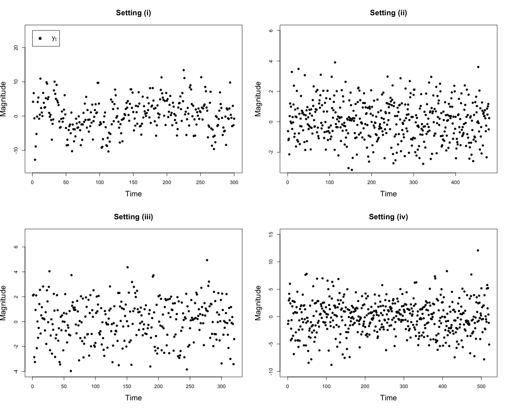
In this section, we conduct extensive numerical experiments to examine the performance of VPWBS, EBSA and WBSSGL in terms of estimation accuracy and computational cost. We design a wide range of simulation settings by varying change size κ\kappa, spacing between change-points Δ\Delta, number of change-points KK, sparsity level 𝔰{\mathfrak{s}}, sample size nn and dimension pp. The variance of noise σε2\sigma_{\varepsilon}^{2} is set at 1 for all settings. For each simulation setting, we repeat the experiments 100 times. The detailed simulation setting is as follows. We further plot typical realizations of {yt}t=1n\{y_{t}\}_{t=1}^{n} for each setting in Figure 2, where it can be seen clearly that information contained in {yt}t=1n\{y_{t}\}_{t=1}^{n} is not sufficient for change-point estimation.

Setting (i): two change-points with varying change size κ\kappa. In this setting, we fix n=300n=300, p=100p=100, K=2K=2 and set the covariance matrix Σ\Sigma of xtx_{t} to be the Toeplitz matrix with Σi,j=0.6|i−j|\Sigma_{i,j}=0.6^{|i-j|} for i,j=1,⋯,pi,j=1,\cdots,p. The two change-points occur at η1=n/3=100\eta_{1}=n/3=100 and η2=2​n/3=200\eta_{2}=2n/3=200. The regression coefficients {βt∗}t=1n\{\beta_{t}^{*}\}_{t=1}^{n} take the form

βt∗={κ⋅α/40, for ​1≤t≤n/3,−κ⋅α/40, for ​n/3+1≤t≤2​n/3,κ⋅α/40, for ​2​n/3+1≤t≤n,\beta_{t}^{*}=\begin{cases}{\kappa}\cdot\alpha/{\sqrt{40}},&\text{ for }1\leq t\leq{n}/{3},\\ -{\kappa}\cdot\alpha/{\sqrt{40}},&\text{ for }{n}/{3}+1\leq t\leq{2n}/{3},\\ {\kappa}\cdot\alpha/{\sqrt{40}},&\text{ for }{2n}/{3}+1\leq t\leq n,\end{cases}

where α=(1,−1,1,−1​…,−1⏟10,0,…,0⏟p−10)\alpha=(\underbrace{1,-1,1,-1\ldots,-1}_{10},\underbrace{0,\ldots,0}_{p-10}) and we vary κ∈40⋅{1,1.2,1.4,1.6}\kappa\in\sqrt{40}\cdot\{1,1.2,1.4,1.6\}. Simple calculation shows that the change size of βt∗\beta_{t}^{*} at both change-points equals κ\kappa.

Setting (ii): three change-points with varying sample size nn. In this setting, we vary n∈{480,560,640,720,800}n\in\{480,560,640,720,800\}, fix p=100p=100, K=3K=3 and set the covariance matrix Σ\Sigma of xtx_{t} to be the identity matrix IpI_{p}. The three change-points occur evenly at ηi=i​n/4\eta_{i}=in/4 for i=1,2,3i=1,2,3. The regression coefficients {βt∗}t=1n\{\beta_{t}^{*}\}_{t=1}^{n} take the form

βt∗={2/5​α, for ​1≤t≤n/4,−2/5α, for ​n/4+1≤t≤n/2,2/5​α, for ​n/2+1≤t≤3​n/4,−2/5α, for ​3​n/4+1≤t≤n,\beta_{t}^{*}=\begin{cases}{2}/{5}\alpha,&\text{ for }1\leq t\leq{n}/{4},\\ -{2}/{5}\alpha,&\text{ for }{n}/{4}+1\leq t\leq{n}/{2},\\ {2}/{5}\alpha,&\text{ for }{n}/{2}+1\leq t\leq{3n}/{4},\\ -{2}/{5}\alpha,&\text{ for }{3n}/{4}+1\leq t\leq n,\end{cases}

where α=(1,−1,1,−1,0,⋯,0)\alpha=(1,-1,1,-1,0,\cdots,0). The change size of βt∗\beta_{t}^{*} at each change-point equals 8/5.8/5.

Setting (iii): two change-points with varying pp and varying support of βt\beta_{t}. In this setting, we fix n=320n=320, K=2K=2, vary p∈{90,100,110,120}p\in\{90,100,110,120\} and set the covariance matrix Σ\Sigma of xtx_{t} to be IpI_{p}. The two change-points occur unevenly at η1=120\eta_{1}=120 and η2=220\eta_{2}=220. The regression coefficients {βt∗}t=1n\{\beta_{t}^{*}\}_{t=1}^{n} take the form

βt∗={2/3⋅(1,…,1⏟8,0,…,0), for ​1≤t≤120,2/3⋅(0,…,0⏟8,1,…,1⏟8,0,…,0), for ​121≤t≤220,2/3⋅(0,…,0⏟16,1,…,1⏟8,0,…,0), for ​221≤t≤320.\beta_{t}^{*}=\begin{cases}{2}/{3}\cdot(\underbrace{1,\ldots,1}_{8},0,\ldots,0),&\text{ for }1\leq t\leq 120,\\ {2}/{3}\cdot(\underbrace{0,\ldots,0}_{8},\underbrace{1,\ldots,1}_{8},0,\ldots,0),&\text{ for }121\leq t\leq 220,\\ {2}/{3}\cdot(\underbrace{0,\ldots,0}_{16},\underbrace{1,\ldots,1}_{8},0,\ldots,0),&\text{ for }221\leq t\leq 320.\end{cases}

Simple calculation shows the change size of βt∗\beta_{t}^{*} at each change-point equals 8/3.8/3.

Setting (iv): two change-points with uneven spacing and varying support size ss. In this setting, we fix n=520n=520, K=2K=2, p=100p=100 and set the covariance matrix of xtx_{t} to be Σ=Ip\Sigma=I_{p}. The two change-points occur unevenly at η1=160\eta_{1}=160 and η2=360\eta_{2}=360. The regression coefficients {βt∗}t=1n\{\beta_{t}^{*}\}_{t=1}^{n} take the form

βt∗={2/s⋅(1,…,1⏟s/2,3,…,3⏟s/2,0,…,0), for ​1≤t≤160,2/s⋅(2,…,2⏟s/2,1,…,1⏟s/2,0,…,0), for ​161≤t≤360,2/s⋅(1,…,1⏟s/2,3,…,3⏟s/2,0,…,0), for ​361≤t≤520,\beta_{t}^{*}=\begin{cases}\sqrt{{2}/{s}}\cdot(\underbrace{1,\ldots,1}_{s/2},\underbrace{3,\ldots,3}_{s/2},0,\ldots,0),&\text{ for }1\leq t\leq 160,\\ \sqrt{{2}/{s}}\cdot(\underbrace{2,\ldots,2}_{s/2},\underbrace{1,\ldots,1}_{s/2},0,\ldots,0),&\text{ for }161\leq t\leq 360,\\ \sqrt{{2}/{s}}\cdot(\underbrace{1,\ldots,1}_{s/2},\underbrace{3,\ldots,3}_{s/2},0,\ldots,0),&\text{ for }361\leq t\leq 520,\end{cases}

and we vary s∈{16,20,24,28}{s}\in\{16,20,24,28\}. Simple calculation shows that the change sizes of βt∗\beta_{t}^{*} at both change-points equal κ=5\kappa=\sqrt{5}.

Refer to caption
Figure 2: Typical realizations of {yt}t=1n\{y_{t}\}_{t=1}^{n} for Setting (i) with κ=40\kappa=\sqrt{40}, Setting (ii) with n=480n=480, Setting (iii) with p=90p=90 and Setting (iv) with κ=0.35​40\kappa=0.35\sqrt{40}.

Estimation accuracy: Table 2 reports the scaled Hausdorff distance (averaged over 100 repetitions) achieved by VPWBS, EBSA and WBSSGL across all simulation settings. For better visualization, Figure 3 further provides the bar plots based on the results reported in Table 2. First, as expected, the performance of all three algorithms improve with larger sample size nn (setting (ii)) and with larger change size κ\kappa (setting (i)), and worsen with higher dimension pp (setting (iii)) and with higher sparsity (setting (iv)).

Overall, VPWBS offers robust and competitive performance for change-point estimation across all simulation settings, and consistently outperforms its competitors under the low SNR scenario where the sample size nn or the change size κ\kappa is small. Compared to WBSSGL, which conducts change-point estimation directly on the estimated {β^t}t=1n\{\widehat{\beta}_{t}\}_{t=1}^{n} by a penalized M-estimator (i.e. SGL), VPWBS in general gives more favorable performance, which could be seen as numerical evidence confirming the importance of the projection step in VPWBS. It is worth noting that when the SNR is large, EBSA becomes highly competitive. We conjecture that EBSA is also minimax optimal when the signal strength Δ​κ2\Delta\kappa^{2} is sufficiently large, though rigorous proof of such result seems challenging.

VPWBS EBSA WBSSGL
Setting (i) κ=40\kappa=\sqrt{40} 0.011 (0.015) 0.090 (0.055) 0.151 (0.094)
κ=1.2​40\kappa=1.2\sqrt{40} 0.009 (0.017) 0.060 (0.052) 0.118 (0.069)
κ=1.4​40\kappa=1.4\sqrt{40} 0.010 (0.024) 0.033 (0.044) 0.101 (0.058)
κ=1.6​40\kappa=1.6\sqrt{40} 0.009 (0.016) 0.025 (0.039) 0.098 (0.061)
Setting (ii) n=480n=480 0.062 (0.080) 0.128 (0.177) 0.101 (0.052)
n=560n=560 0.044 (0.042) 0.064 (0.112) 0.098 (0.053)
n=640n=640 0.034 (0.060) 0.034 (0.084) 0.094 (0.055)
n=720n=720 0.026 (0.054) 0.015 (0.023) 0.093 (0.075)
n=800n=800 0.022 (0.046) 0.009 (0.010) 0.091 (0.072)
Setting (iii) p=80p=80 0.025 (0.047) 0.052 (0.047) 0.103 (0.065)
p=90p=90 0.039 (0.068) 0.068 (0.051) 0.109 (0.068)
p=100p=100 0.033 (0.056) 0.056 (0.050) 0.120 (0.072)
p=110p=110 0.041 (0.063) 0.055 (0.046) 0.125 (0.072)
p=120p=120 0.049 (0.078) 0.061 (0.048) 0.140 (0.079)
Setting (iv) s=16s=16 0.027 (0.072) 0.055 (0.023) 0.116 (0.059)
s=20s=20 0.024 (0.060) 0.059 (0.024) 0.141 (0.033)
s=24s=24 0.043 (0.089) 0.057 (0.020) 0.141 (0.032)
s=28s=28 0.057 (0.106) 0.063 (0.022) 0.144 (0.023)
Table 2: Scaled Hausdorff distance for VPWBS, EBSA (Leonardi and Bühlmann 2016) and WBSSGL (Zhang et al. 2015b). For each cell, the experiment is repeated 100 times. The numbers in the brackets indicate the sample standard errors of the scaled Hausdorff distance. Each highlighted number indicates the best performance in the corresponding setting.
Refer to caption
Figure 3: Bar plots for estimation results reported in Table 2. Plots 1-4 correspond to Setting (i) with κ∈40⋅{1,1.2,1.4,1.6}\kappa\in\sqrt{40}\cdot\{1,1.2,1.4,1.6\}. Plots 5-9 correspond to Setting (ii) with n∈{480,560,640,720,800}n\in\{480,560,640,720,800\}. Plots 10-14 correspond to Setting (iii) with p∈{80,90,100,110,120}p\in\{80,90,100,110,120\}. Plots 15-18 correspond to Setting (iv) with s∈{16,20,24,28}s\in\{16,20,24,28\}.

Computational cost: It is straightforward to derive that the computational cost of VPWBS is O​(M​n⋅GroupLasso​(n,p))O(Mn\cdot\text{GroupLasso}(n,p)), where MM is the number of random intervals used and recall that GroupLasso​(n,p)\text{GroupLasso}(n,p) denotes the computational cost of the group Lasso for a pp-dimensional regression with nn samples. Since we set M=(log⁡(n))2M=(\log(n))^{2}, the computational complexity of VPWBS equals O⁡(n​(log⁡(n))2⋅GroupLasso​(n,p))O(n(\log(n))^{2}\cdot\text{GroupLasso}(n,p)). On the other hand, referring to Table 1, the complexity of EBSA and WBSSGL are O⁡(n​log⁡(n)⋅Lasso​(n,p))O(n\log(n)\cdot\text{Lasso}(n,p)) and O​(Lasso​(n,n​p))O(\text{Lasso}(n,np)) respectively.

Note that the computational cost of solving Lasso and group Lasso for a pp-dimensional linear regression with nn observations is both O⁡(n​p2)O(np^{2}), see for example Efron et al. 2004 and Wright et al. 2009. Thus, it is easy to see that in terms of computational efficiency, ESBA is the best, VPWBS comes second, and WBSSGL comes last. In practice, popular R packages typically implement gradient or coordinate descent to obtain an approximate solution of Lasso and group Lasso and the computation can be much faster than O⁡(n​p2)O(np^{2}).

We conduct further numerical experiments to exam the computational performance of each algorithm in practice. Specifically, given (n,p)(n,p), we generate the regression coefficients {βt∗}t=1n\{\beta_{t}^{*}\}_{t=1}^{n} and observations {xt,yt}t=1n\{x_{t},y_{t}\}_{t=1}^{n} using Setting (i) with κ=1.6​40\kappa=1.6\sqrt{40}. In the first set of experiments, we fix n=450n=450 and vary p∈{80,100,120,140,160,180,200,220}p\in\{80,100,120,140,160,180,200,220\}; in the second set of experiments, we fix p=100p=100 and vary n∈{240,300,360,420,480,540,600,660}n\in\{240,300,360,420,480,540,600,660\}. For each simulation setting, we repeat the experiments 100 times and report the average execution time of VPWBS, EBSA and WBSSGL in Figure 4.

As can be seen in Figure 4, the computational costs of VPWBS and EBSA increase linearly with both the dimension pp and the sample size nn. On the other hand, while the computational cost of WBSSGL grows linearly with pp, it does not scale well with nn. This is not surprising, as the SGL approach (7) is essentially solving a Lasso with nn samples and n​pnp covariates.

Refer to caption
Figure 4: Average execution time of VPWBS, EBSA and WBSSGL across different simple sizes nn and dimensions pp.

5 Discussion

In this paper, we study the problem of multiple change-point estimation in high-dimensional linear regression model. We propose a novel projection-based algorithm, VPWBS, which performs change-point detection from a dimension reduction angle. Based on an estimated (optimal) projection direction, VPWBS transforms the original (difficult) problem of change-point detection in pp-dimensional regression to a simpler problem of change-point detection in mean of a one-dimensional time series. VPWBS is shown to achieve the minimax optimal localization rate Op​(1/n)O_{p}(1/n) up to a log factor, a significant improvement from the best rate Op​(1/n)O_{p}(1/\sqrt{n}) known in the existing literature. In addition, VPWBS is computationally efficient with a complexity of O⁡(n​(log⁡(n))2⋅GroupLasso​(n,p))O(n(\log(n))^{2}\cdot\text{GroupLasso}(n,p)). Extensive numerical experiments are conducted to demonstrate the robust and favorable performance of VPWBS over two state-of-the-art algorithms in a wide range of simulation settings.

Besides the high-dimensional regression problem, we believe the projection based change-point estimation framework can be useful under other important contexts as well, such as change in covariance matrices and tensors. The key is to design an algorithm that utilizes the structure of the specific problem (such as sparsity or low rank) and provides a provably accurate estimation of the (optimal) projection direction.

Acknowledgments

We would like to thank the editor, Dr. Zaid Harchaoui, as well as the three anonymous reviewers for their thoughtful assessment and constructive comments which helped us to improve the quality and the presentation of our paper. The work of RW was supported in part by AFOSR FA9550-18-1-0166, NSF DMS-1925101, NSF OAC-1934637, and DOE DE-AC02-06CH11357.

References

  • Bai and Perron (1998) Jushan Bai and Pierre Perron. Estimating and testing linear models with multiple structural changes. Econometrica, pages 47–78, 1998.
  • Bleakley and Vert (2011) Kevin Bleakley and Jean-Philippe Vert. The group fused lasso for multiple change-point detection. Technical report HAL-00602121, 2011.
  • Cai and Guo (2020) T. Tony Cai and Zijian Guo. Semi-supervised inference for explained variance in high-dimensional linear regression and its applications. Journal of the Royal Statistical Society: Series B, 82(2):391–419, 2020.
  • Castro et al. (2018) Bruno M Castro, Renan B Lemes, Jonatas Cesar, Tábita Hünemeier, and Florencia Leonardi. A model selection approach for multiple sequence segmentation and dimensionality reduction. Journal of Multivariate Analysis, 167:319–330, 2018.
  • Chen and Gupta (1997) Jie Chen and Arjun K Gupta. Testing and locating variance changepoints with application to stock prices. Journal of the American Statistical association, 92(438):739–747, 1997.
  • Cho and Fryzlewicz (2015) Haeran Cho and Piotr Fryzlewicz. Multiple-change-point detection for high dimensional time series via sparsified binary segmentation. Journal of the Royal Statistical Society: Series B (Statistical Methodology), 77(2):475–507, 2015.
  • Cho et al. (2016) Haeran Cho et al. Change-point detection in panel data via double cusum statistic. Electronic Journal of Statistics, 10(2):2000–2038, 2016.
  • Cribben and Yu (2017) Ivor Cribben and Yi Yu. Estimating whole-brain dynamics by using spectral clustering. Journal of the Royal Statistical Society: Series C (Applied Statistics), 66(3):607–627, 2017.
  • Efron et al. (2004) Bradley Efron, Trevor Hastie, Iain Johnstone, and Robert Tibshirani. Least angle regression. The Annals of Statistics, 32(2):407–499, 2004.
  • Enikeeva and Harchaoui (2019) Farida Enikeeva and Zaid Harchaoui. High-dimensional change-point detection under sparse alternatives. The Annals of Statistics, 47(4):2051–2079, 2019.
  • Frick et al. (2014) Klaus Frick, Axel Munk, and Hannes Sieling. Multiscale change point inference. Journal of the Royal Statistical Society: Series B (Statistical Methodology), 76(3):495–580, 2014.
  • Fryzlewicz (2014) Piotr Fryzlewicz. Wild binary segmentation for multiple change-point detection. The Annals of Statistics, 42(6):2243–2281, 2014.
  • Harchaoui and Lévy-Leduc (2007) Zaid Harchaoui and Céline Lévy-Leduc. Catching change-points with lasso. Advances inNeural Information Processing Systems 20, 2007.
  • Harchaoui and Lévy-Leduc (2010) Zaid Harchaoui and Céline Lévy-Leduc. Multiple change-point estimation with a total-variation penalty. Journal of the American Statistical Association, 105(492):1480–1493, 2010.
  • Hušková et al. (2007) Marie Hušková, Zuzana Prášková, and Josef Steinebach. On the detection of changes in autoregressive time series i. asymptotics. Journal of Statistical Planning and Inference, 137(4):1243–1259, 2007.
  • Jiang et al. (2021) Feiyu Jiang, Zifeng Zhao, and Xiaofeng Shao. Modelling the covid‐19 infection trajectory: A piecewise linear quantile trend model. Journal of the Royal Statistical Society: Series B, 2021.
  • Kaul et al. (2019) Abhishek Kaul, Venkata K Jandhyala, and Stergios B Fotopoulos. An efficient two step algorithm for high dimensional change point regression models without grid search. Journal of Machine Learning Research, (20):1–40, 2019.
  • Lee et al. (2016) Sokbae Lee, Myung Hwan Seo, and Youngki Shin. The lasso for high dimensional regression with a possible change point. Journal of the Royal Statistical Society: Series B (Statistical Methodology), 78(1):193–210, 2016.
  • Lee et al. (2018) Sokbae Lee, Yuan Liao, Myung Hwan Seo, and Youngki Shin. Oracle estimation of a change point in high-dimensional quantile regression. Journal of the American Statistical Association, 113(523):1184–1194, 2018.
  • Leonardi and Bühlmann (2016) Florencia Leonardi and Peter Bühlmann. Computationally efficient change point detection for high-dimensional regression. arXiv preprint arXiv:1601.03704, 2016.
  • Li et al. (2021) Yu-Ning Li, Degui Li, and Piotr Fryzlewicz. Detection of multiple structural breaks in largecovariance matrices. Working paper, 2021.
  • Owrang et al. (2017) Arash Owrang, Mohammadreza Malek-Mohammadi, Alexandre Proutiere, and Magnus Jansson. Consistent change point detection for piecewise constant signals with normalized fused lasso. IEEE Signal Processing Letters, 24(6):799 – 803, 2017.
  • Pein et al. (2017) Florian Pein, Hannes Sieling, and Axel Munk. Heterogeneous change point inference. Journal of the Royal Statistical Society: Series B (Statistical Methodology), 79(4):1207–1227, 2017.
  • Peng et al. (2004) Tao Peng, Christopher Leckie, and Kotagiri Ramamohanarao. Proactively detecting distributed denial of service attacks using source ip address monitoring. In International conference on research in networking, pages 771–782. Springer, 2004.
  • Qu and Perron (2007) Zhongjun Qu and Pierre Perron. Estimating and testing structural changes in multivariate regressions. Econometrica, 75(2):459–502, 2007.
  • Raskutti et al. (2010) Garvesh Raskutti, Martin J Wainwright, and Bin Yu. Restricted eigenvalue properties for correlated gaussian designs. Journal of Machine Learning Research, 11(Aug):2241–2259, 2010.
  • Richard A. Davis (1995) Yi-Ching Yao Richard A. Davis, Dawei Huang. Testing for a change in the parameter values and order of an autoregressive model. The Annals of Statistics, 23(1):282–304, 1995.
  • Rojas and Wahlberg (2014) Cristian R. Rojas and Bo Wahlberg. On change point detection using the fused lasso method. arXiv:1401.5408, 2014.
  • Simon et al. (2013) Noah Simon, Jerome Friedman, Trevor Hastie, and Robert Tibshirani. A sparse-group lasso. Journal of Computational and Graphical Statistics, 22(2):231–245, 2013.
  • Wang et al. (2017) Daren Wang, Yi Yu, and Alessandro Rinaldo. Optimal covariance change point localization in high dimension. arXiv preprint arXiv:1712.09912, 2017.
  • Wang et al. (2018) Daren Wang, Yi Yu, and Alessandro Rinaldo. Univariate mean change point detection: Penalization, cusum and optimality. arXiv preprint arXiv:1810.09498, 2018.
  • Wang et al. (2021) Daren Wang, Yi Yu, and Alessandro Rinaldo. Optimal change point detection and localization in sparse dynamic networks. The Annals of Statistics, 49(1):203–232, 2021.
  • Wang and Samworth (2018) Tengyao Wang and Richard J Samworth. High dimensional change point estimation via sparse projection. Journal of the Royal Statistical Society: Series B (Statistical Methodology), 80(1):57–83, 2018.
  • Wright et al. (2009) Stephen J. Wright, Robert D. Nowak, and MÁrio A. T. Figueiredo. Sparse reconstruction by separable approximation. IEEE Transactions on Signal Processing, 57(7):2479 – 2493, 2009.
  • Xie et al. (2020) Liyan Xie, Yao Xie, and George V Moustakides. Sequential subspace change point detection. Sequential Analysis, 39(3):307–335, 2020.
  • Yau and Zhao (2016) Chun Yip Yau and Zifeng Zhao. Inference for multiple change points in time series via likelihood ratio scan statistics. Journal of the Royal Statistical Society: Series B, 78(4):895–916, 2016.
  • Zhang et al. (2015a) Bingwen Zhang, Jun Geng, and Lifeng Lai. Change-point estimation in high dimensional linear regression models via sparse group lasso. In Communication, Control, and Computing (Allerton), 2015 53rd Annual Allerton Conference on, pages 815–821. IEEE, 2015a.
  • Zhang et al. (2015b) Bingwen Zhang, Jun Geng, and Lifeng Lai. Multiple change-points estimation in linear regression models via sparse group lasso. IEEE Trans. Signal Processing, 63(9):2209–2224, 2015b.
  • Zhao and Yau (2021) Zifeng Zhao and Chun Yip Yau. Alternating pruned dynamic programming for multiple epidemic change-point estimation. Journal of Computational and Graphical Statistics, 30(3):808–821, 2021.
  • Zhao et al. (2019) Zifeng Zhao, Li Chen, and Lizhen Lin. Change-point detection in dynamic networks via graphon estimation. arXiv:1908.01823, 2019.
  • Zou et al. (2020) Changliang Zou, Guanghui Wang, and Runze Li. Consistent selection of the number of change-points via sample-splitting. The Annals of Statistics, 48(1):413–439, 2020.

Appendix A Proofs Related to Theorem 2

In this section, we provide all the technical details for the proof of Theorem 2

Proof of Theorem 2 .

Denote

κ′=‖βη∗−βη+1∗‖2.\kappa^{\prime}=\|\beta^{*}_{\eta}-\beta^{*}_{\eta+1}\|_{2}.

Since (α^1,α^2,ν^)\left(\widehat{\alpha}_{1},\widehat{\alpha}_{2},\widehat{\nu}\right) be the output of LGS ({yi,xi}i=1n,(s,e],λ)(\{y_{i},x_{i}\}_{i=1}^{n},(s,e],\lambda), it holds that

(α^1,α^2)=arg​minα1,α2∈ℝp{\displaystyle(\widehat{\alpha}_{1},\widehat{\alpha}_{2})=\argmin_{\alpha_{1},\alpha_{2}\in\mathbb{R}^{p}}\Bigg\{ ∑i=s+1ν^(yi−xi⊤​α1)2+∑i=ν^+1e(yi−xi⊤​α2)2\displaystyle\sum_{i=s+1}^{\widehat{\nu}}(y_{i}-x_{i}^{\top}\alpha_{1}\bigr)^{2}+\sum_{i=\widehat{\nu}+1}^{e}(y_{i}-x^{\top}_{i}\alpha_{2})^{2}
+\displaystyle+ λ∑j=1p(ν^−s)​(α1,j)2+(e−ν^)​(α2,j)2},\displaystyle\lambda\sum_{j=1}^{p}\sqrt{(\widehat{\nu}-s)(\alpha_{1,j})^{2}+(e-\widehat{\nu})(\alpha_{2,j})^{2}}\Bigg\}\ ,

and that by Lemma 4,

|η−ν^|≤C​𝔰​log⁡(p​n)(κ′)2.|\eta-\widehat{\nu}|\leq C\frac{{\mathfrak{s}}\log(pn)}{(\kappa^{{}^{\prime}})^{2}}.

Without loss of generality, assume that s<η<ν^≤e.s<\eta<\widehat{\nu}\leq e. Then by Lemma 5,

‖α^1−β(s,ν^]∗‖22≤C​𝔰​log⁡(p​n)Δ≤C​𝔰​log⁡(p​n)Cs​n​r​𝔰​log⁡(p​n)​κ−2≤C​κ2Cs​n​r≤C​(κ′)2Cs​n​r,\big\|\widehat{\alpha}_{1}-\beta^{*}_{(s,\widehat{\nu}]}\big\|_{2}^{2}\leq C\frac{{\mathfrak{s}}\log(pn)}{\Delta}\leq\frac{C{\mathfrak{s}}\log(pn)}{C_{snr}{\mathfrak{s}}\log(pn)\kappa^{-2}}\leq\frac{C\kappa^{2}}{C_{snr}}\leq\frac{C(\kappa^{\prime})^{2}}{C_{snr}},

For sufficient large constant Cs​n​rC_{snr}, it holds that

‖α^1−β(s,ν^]∗‖2≤cx128​Cx​κ′and‖α^2−β(ν^,e]∗‖2≤cx128​Cx​κ′.\big\|\widehat{\alpha}_{1}-\beta^{*}_{(s,\widehat{\nu}]}\big\|_{2}\leq\frac{c_{x}}{128C_{x}}\kappa^{\prime}\quad\text{and}\quad\big\|\widehat{\alpha}_{2}-\beta^{*}_{(\widehat{\nu},e]}\big\|_{2}\leq\frac{c_{x}}{128C_{x}}\kappa^{\prime}.

Since β(ν^,e]∗=βη+1∗,\beta^{*}_{(\widehat{\nu},e]}=\beta_{\eta+1}^{*}, it follows that

‖α^2−βη+1∗‖2≤cx128​Cx​κ′.\displaystyle\big\|\widehat{\alpha}_{2}-\beta^{*}_{\eta+1}\big\|_{2}\leq\frac{c_{x}}{128C_{x}}\kappa^{\prime}. (9)

Note that

‖α^1−β(s,ν^]∗‖2=\displaystyle\big\|\widehat{\alpha}_{1}-\beta^{*}_{(s,\widehat{\nu}]}\big\|_{2}= ‖α^1−(s−η)​βη∗+(ν^−η)​βη+1∗ν^−s‖2\displaystyle\bigg\|\widehat{\alpha}_{1}-\frac{(s-\eta)\beta^{*}_{\eta}+(\widehat{\nu}-\eta)\beta^{*}_{\eta+1}}{\widehat{\nu}-s}\bigg\|_{2}
≥\displaystyle\geq ‖α^1−βη∗‖2−‖βη∗−(s−η)​βη∗+(ν^−η)​βη+1∗ν^−s‖2\displaystyle\|\widehat{\alpha}_{1}-\beta_{\eta}^{*}\|_{2}-\bigg\|\beta_{\eta}^{*}-\frac{(s-\eta)\beta^{*}_{\eta}+(\widehat{\nu}-\eta)\beta^{*}_{\eta+1}}{\widehat{\nu}-s}\bigg\|_{2}
≥\displaystyle\geq ‖α^1−βη∗‖2−ν^−ην^−s​‖βη∗−βη+1∗‖2\displaystyle\|\widehat{\alpha}_{1}-\beta_{\eta}^{*}\|_{2}-\frac{\widehat{\nu}-\eta}{\widehat{\nu}-s}\|\beta_{\eta}^{*}-\beta^{*}_{\eta+1}\|_{2}
≥\displaystyle\geq ‖α^1−βη∗‖2−C𝔰log(pn)/(κ′)2120​Cs​n​r​𝔰​log⁡(p​n)/κ2​(κ′)\displaystyle\|\widehat{\alpha}_{1}-\beta_{\eta}^{*}\|_{2}-\frac{C{\mathfrak{s}}\log(pn)/(\kappa^{{}^{\prime}})^{2}}{{\frac{1}{20}}C_{snr}{\mathfrak{s}}\log(pn)/\kappa^{2}}(\kappa^{\prime})
≥\displaystyle\geq ‖α^1−βη∗‖2−cx128​Cx​κ2κ′\displaystyle\|\widehat{\alpha}_{1}-\beta_{\eta}^{*}\|_{2}-\frac{c_{x}}{128C_{x}}\frac{\kappa^{2}}{\kappa^{\prime}}
≥\displaystyle\geq ‖α^1−βη∗‖2−cx128​Cx​κ′,\displaystyle\|\widehat{\alpha}_{1}-\beta_{\eta}^{*}\|_{2}-\frac{c_{x}}{128C_{x}}\kappa^{\prime},

where the third inequality follows from the fact that ν^−s≥e−s10≥Δ20≥120​Cs​n​r​κ−2​𝔰​log⁡(p​n)\widehat{\nu}-s\geq\frac{e-s}{10}\geq\frac{\Delta}{20}\geq\frac{1}{20}C_{snr}\kappa^{-2}{\mathfrak{s}}\log(pn) and the fourth inequality holds if Cs​n​rC_{snr} is sufficiently large. As a result

‖α^1−βη∗‖2≤cx64​Cx​κ′.\displaystyle\|\widehat{\alpha}_{1}-\beta_{\eta}^{*}\|_{2}\leq\frac{c_{x}}{64C_{x}}\kappa^{\prime}. (10)

The desired result is an immediate consequence of Equation 9 and Equation 10. ∎

Lemma 4.

Suppose that [s+1,e]⊂[1,n][s+1,e]\subset[1,n] is any interval such that e−s≥Δ2e-s\geq\frac{\Delta}{2} and that [s+1,e][s+1,e] contains exactly one change point η\eta which satisfies

min⁡{η−s,e−η}≥e−s10.\min\{\eta-s,e-\eta\}\geq\frac{e-s}{10}.

Suppose Assumptions 1-2.2 hold and λ=Cλ​log⁡(p​n)\lambda=C_{\lambda}\sqrt{\log(pn)} for a sufficiently large constant CλC_{\lambda}. Let (α^1,α^2,ν^)\left(\widehat{\alpha}_{1},\widehat{\alpha}_{2},\widehat{\nu}\right) be the output of LGS ({yi,xi}i=1n,(s,e],λ)(\{y_{i},x_{i}\}_{i=1}^{n},(s,e],\lambda). Denote

κ′=‖βη∗−βη+1∗‖2.\kappa^{\prime}=\|\beta^{*}_{\eta}-\beta^{*}_{\eta+1}\|_{2}.

Then with probability at least 1−(p​n)−41-(pn)^{-4}, it holds that

|η−ν^|≤C​𝔰​log⁡(p​n)(κ′)2.|\eta-\widehat{\nu}|\leq C\frac{{\mathfrak{s}}\log(pn)}{(\kappa^{{}^{\prime}})^{2}}.
Proof of Lemma 4.

Let S1S_{1} be the support of βi∗\beta_{i}^{*} when i∈(s,η]i\in(s,\eta] and S2S_{2} be the support of βi∗\beta_{i}^{*} when i∈(η,e]i\in(\eta,e]. Denote

S=S1∪S2.S=S_{1}\cup S_{2}.

Note that |S|≤2​𝔰|S|\leq 2{\mathfrak{s}} and that SS is the common support for βi∗\beta_{i}^{*} for i∈(s,e]i\in(s,e]. Without loss of generality, we assume that s<η<ν^<es<\eta<\widehat{\nu}<e. Denote

β^i={α^1,i∈(s,ν^],α^2,i∈(ν^,e].\widehat{\beta}_{i}=\begin{cases}\widehat{\alpha}_{1},&i\in(s,\widehat{\nu}],\\ \widehat{\alpha}_{2},&i\in(\widehat{\nu},e].\end{cases}

If ν^−η<C1​𝔰​log⁡(p​n)κ2\widehat{\nu}-\eta<C_{1}\frac{{\mathfrak{s}}\log(pn)}{\kappa^{2}} for some sufficiently large constant C1C_{1}, then the desired result holds.

So suppose that

ν^−η≥C1​𝔰​log⁡(p​n)κ2.\displaystyle\widehat{\nu}-\eta\geq C_{1}\frac{{\mathfrak{s}}\log(pn)}{\kappa^{2}}. (11)

Note that since κ<Cκ<∞\kappa<C_{\kappa}<\infty, Equation 11 implies that

ν^−η≥C1​Cκ−2​𝔰​log⁡(p​n).\displaystyle\widehat{\nu}-\eta\geq C_{1}C_{\kappa}^{-2}{\mathfrak{s}}\log(pn). (12)

By assumption,

min⁡{η−s,e−ν^}≥e−s10≥Δ20≥120​Cs​n​r​Cκ−2​𝔰​log⁡(p​n).\displaystyle\min\{\eta-s,e-\widehat{\nu}\}\geq\frac{e-s}{10}\geq\frac{\Delta}{20}\geq\frac{1}{20}C_{snr}C_{\kappa}^{-2}{\mathfrak{s}}\log(pn). (13)


Step 1. In this step, it is shown that with probability at least 1−C​(n​p)−51-C(np)^{-5},

∑i=s+1e‖β^i−βi∗‖22≤C3​𝔰​λ2.\sum_{i=s+1}^{e}\|\widehat{\beta}_{i}-\beta^{*}_{i}\|_{2}^{2}\leq C_{3}{\mathfrak{s}}\lambda^{2}.

From Equation 4, it holds that

∑i=s+1e(yi−xi⊤​β^i)2+λ​∑j=1p∑i=s+1e(β^i,j)2≤∑i=s+1e(yi−xi⊤​βi∗)2+λ​∑j=1p∑i=s+1e(βi,j∗)2.\displaystyle\sum_{i=s+1}^{e}(y_{i}-x_{i}^{\top}\widehat{\beta}_{i})^{2}+\lambda\sum_{j=1}^{p}\sqrt{\sum_{i=s+1}^{e}\bigl(\widehat{\beta}_{i,j}\bigr)^{2}}\leq\sum_{i=s+1}^{e}(y_{i}-x_{i}^{\top}\beta^{*}_{i})^{2}+\lambda\sum_{j=1}^{p}\sqrt{\sum_{i=s+1}^{e}\bigl(\beta^{*}_{i,j}\bigr)^{2}}. (14)

Let δi=β^i−βi∗\delta_{i}=\widehat{\beta}_{i}-\beta^{*}_{i}. It holds that

∑i=s+1e−1𝟙{δi≠δi+1}=2.\sum_{i=s+1}^{e-1}\mathbbm{1}\left\{\delta_{i}\neq\delta_{i+1}\right\}=2.

Equation 14 implies that

∑i=s+1e‖δi⊤​xi‖22+λ​∑j=1p∑i=s+1e(β^i,j)2≤2​∑i=s+1e(yi−xi⊤​βi∗)​δi⊤​xi+λ​∑j=1p∑i=s+1e(βi,j∗)2.\displaystyle\sum_{i=s+1}^{e}\|\delta_{i}^{\top}x_{i}\|_{2}^{2}+\lambda\sum_{j=1}^{p}\sqrt{\sum_{i=s+1}^{e}\bigl(\widehat{\beta}_{i,j}\bigr)^{2}}\leq 2\sum_{i=s+1}^{e}(y_{i}-x_{i}^{\top}\beta^{*}_{i})\delta_{i}^{\top}x_{i}+\lambda\sum_{j=1}^{p}\sqrt{\sum_{i=s+1}^{e}\bigl(\beta^{*}_{i,j}\bigr)^{2}}. (15)


Note that since SS is the common support for βi∗\beta_{i}^{*} for i∈(s,e]i\in(s,e], it holds that

∑j=1p∑i=s+1e(βi,j∗)2−∑j=1p∑i=s+1e(β^i,j)2\displaystyle\sum_{j=1}^{p}\sqrt{\sum_{i=s+1}^{e}\bigl(\beta^{*}_{i,j}\bigr)^{2}}-\sum_{j=1}^{p}\sqrt{\sum_{i=s+1}^{e}\bigl(\widehat{\beta}_{i,j}\bigr)^{2}}
=\displaystyle= ∑j∈S∑i=s+1e(βi,j∗)2−∑j∈S∑i=s+1e(β^i,j)2−∑j∈Sc∑i=s+1e(β^i,j)2\displaystyle\sum_{j\in S}\sqrt{\sum_{i=s+1}^{e}\bigl(\beta^{*}_{i,j}\bigr)^{2}}-\sum_{j\in S}\sqrt{\sum_{i=s+1}^{e}\bigl(\widehat{\beta}_{i,j}\bigr)^{2}}-\sum_{j\in S^{c}}\sqrt{\sum_{i=s+1}^{e}\bigl(\widehat{\beta}_{i,j}\bigr)^{2}}
≤\displaystyle\leq ∑j∈S∑i=s+1e(δi,j)2−∑j∈Sc∑i=s+1e(δi,j)2.\displaystyle\sum_{j\in S}\sqrt{\sum_{i=s+1}^{e}\bigl(\delta_{i,j}\bigr)^{2}}-\sum_{j\in S^{c}}\sqrt{\sum_{i=s+1}^{e}\bigl(\delta_{i,j}\bigr)^{2}}. (16)

Note that for any j∈[1,…,p]j\in[1,\ldots,p], from Equation 12, Equation 13 and Lemma 8, it holds that

sups<i≤eδi,j∑i=s+1e(δi,j)2≤C4​1𝔰​log⁡(p​n).\displaystyle\sup_{s<i\leq e}\frac{\delta_{i,j}}{\sqrt{\sum_{i=s+1}^{e}\left(\delta_{i,j}\right)^{2}}}\leq C_{4}\frac{1}{\sqrt{{\mathfrak{s}}\log(pn)}}. (17)

As a result, with probability at least 1−(n​p)−51-(np)^{-5}

|∑i=s+1e(yi−xi⊤​βi∗)​δi⊤​xi|=|∑i=s+1eεi​δi⊤​xi|=|∑j=1p{(∑i=s+1eεi​δi,j​xi,j∑i=s+1e(δi,j)2)​∑i=s+1e(δi,j)2}|\displaystyle\left|\sum_{i=s+1}^{e}(y_{i}-x_{i}^{\top}\beta^{*}_{i})\delta_{i}^{\top}x_{i}\right|=\left|\sum_{i=s+1}^{e}\varepsilon_{i}\delta_{i}^{\top}x_{i}\right|=\bigg|\sum_{j=1}^{p}\left\{\left(\frac{\sum_{i=s+1}^{e}\varepsilon_{i}\delta_{i,j}x_{i,j}}{\sqrt{\sum_{i=s+1}^{e}\left(\delta_{i,j}\right)^{2}}}\right)\sqrt{\sum_{i=s+1}^{e}\left(\delta_{i,j}\right)^{2}}\right\}\bigg|
≤\displaystyle\leq supj=1,…,p|∑i=s+1eεi​δi,j​xi,j∑i=s+1e(δi,j)2|​∑j=1p∑i=s+1e(δi,j)2≤C5​log⁡(p​n)​∑j=1p∑i=s+1e(δi,j)2\displaystyle\sup_{j=1,\ldots,p}\left|\frac{\sum_{i=s+1}^{e}\varepsilon_{i}\delta_{i,j}x_{i,j}}{\sqrt{\sum_{i=s+1}^{e}\left(\delta_{i,j}\right)^{2}}}\right|\sum_{j=1}^{p}\sqrt{\sum_{i=s+1}^{e}\left(\delta_{i,j}\right)^{2}}\leq C_{5}\sqrt{\log(pn)}\sum_{j=1}^{p}\sqrt{\sum_{i=s+1}^{e}\left(\delta_{i,j}\right)^{2}}
≤\displaystyle\leq (λ/4)​∑j=1p∑i=s+1e(δi,j)2,\displaystyle(\lambda/4)\sum_{j=1}^{p}\sqrt{\sum_{i=s+1}^{e}\left(\delta_{i,j}\right)^{2}}, (18)

where the second inequality follows from Lemma 7 and Equation 17 if C5C_{5} is a sufficiently large constant, and the last inequality follows from λ=Cλ​log⁡(p​n)\lambda=C_{\lambda}\sqrt{\log(pn)}.
Combining (14), (15), (16) and (18) yields

∑i=s+1e(δi⊤​xi)2+λ2​∑j∈Sc∑i=s+1e(δi,j)2≤3​λ2​∑j∈S∑i=s+1e(δi,j)2.\sum_{i=s+1}^{e}(\delta_{i}^{\top}x_{i})^{2}+\frac{\lambda}{2}\sum_{j\in S^{c}}\sqrt{\sum_{i=s+1}^{e}\bigl(\delta_{i,j}\bigr)^{2}}\leq\frac{3\lambda}{2}\sum_{j\in S}\sqrt{\sum_{i=s+1}^{e}\bigl(\delta_{i,j}\bigr)^{2}}. (19)


Step 2. To apply restricted eigenvalue conditions, let

I=(s,e],I1=(s,η],I2=(η,ν^],I3=(ν^,e].I=(s,e],\quad I_{1}=(s,\eta],\quad I_{2}=(\eta,\widehat{\nu}],\quad I_{3}=(\widehat{\nu},e].

Denote

ℰI:={v⊤(1|I|∑i∈Ixixi⊤)v≥116v⊤Σv−Crlog⁡(p)|I|∥v∥12}.\mathcal{E}_{I}:=\Bigg\{v^{\top}\bigg(\frac{1}{|I|}\sum_{i\in I}x_{i}x_{i}^{\top}\bigg)v\geq\frac{1}{16}v^{\top}\Sigma v-C_{r}\frac{\log(p)}{|I|}\|v\|_{1}^{2}\Bigg\}.

If C1C_{1} in Equation 12 and Cs​n​rC_{snr} in Equation 13 are sufficiently large constants, it holds that

min⁡{|I1|,|I2|,|I3|}≥C6​𝔰​log⁡(n​p)\displaystyle\min\{|I_{1}|,\ |I_{2}|,\ |I_{3}|\}\geq C_{6}{\mathfrak{s}}\log(np) (20)

for some sufficiently large C6C_{6}. For h=1,2,3h=1,2,3, denote ℰIh\mathcal{E}_{I_{h}} the same way as ℰI\mathcal{E}_{I}. So by Theorem 9, P⁡(ℰIh)≥1−(n​p)−5P(\mathcal{E}_{I_{h}})\geq 1-(np)^{-5} for h=1,2,3h=1,2,3. Denote δIh=δi\delta_{I_{h}}=\delta_{i} for any i∈Ihi\in I_{h}. With probability at least 1−3​(n​p)−51-3(np)^{-5}, on the event ⋂h=1,2,3ℰIh\bigcap_{h=1,2,3}\mathcal{E}_{I_{h}},

∑i=s+1e(δi⊤​xi)2=∑h=1,2,3∑i∈Ih(δIh⊤​xi)2\displaystyle\sum_{i=s+1}^{e}(\delta_{i}^{\top}x_{i})^{2}=\sum_{h=1,2,3}\sum_{i\in I_{h}}(\delta_{I_{h}}^{\top}x_{i})^{2}
≥\displaystyle\geq ∑h=1,2,3|Ih|16​δIh⊤​Σ​δIh−Cr​log⁡(p)​‖δIh‖12\displaystyle\sum_{h=1,2,3}\frac{|I_{h}|}{16}\delta_{I_{h}}^{\top}\Sigma\delta_{I_{h}}-C_{r}\log(p)\|\delta_{I_{h}}\|_{1}^{2}
=\displaystyle= ∑h=1,2,3|Ih|16​δIh⊤​Σ​δIh−Cr​log⁡(p)​(‖δIh​(S)‖1+‖δIh​(Sc)‖1)2\displaystyle\sum_{h=1,2,3}\frac{|I_{h}|}{16}\delta_{I_{h}}^{\top}\Sigma\delta_{I_{h}}-C_{r}\log(p)\big(\|\delta_{I_{h}}(S)\|_{1}+\|\delta_{I_{h}}(S^{c})\|_{1}\big)^{2}
≥\displaystyle\geq ∑h=1,2,3cx​|Ih|16​‖δIh‖22−2​Cr​|S|​log⁡(p)​‖δIh‖22−2​Cr​log⁡(p)​‖δIh​(Sc)‖12\displaystyle\sum_{h=1,2,3}\frac{c_{x}|I_{h}|}{16}\|\delta_{I_{h}}\|_{2}^{2}-2C_{r}|S|\log(p)\|\delta_{I_{h}}\|_{2}^{2}-2C_{r}\log(p)\|\delta_{I_{h}}(S^{c})\|_{1}^{2}
≥\displaystyle\geq ∑h=1,2,3cx​|Ih|20​‖δIh‖22−2​Cr​log⁡(p)​‖δIh​(Sc)‖12,\displaystyle\sum_{h=1,2,3}\frac{c_{x}|I_{h}|}{20}\|\delta_{I_{h}}\|_{2}^{2}-2C_{r}\log(p)\|\delta_{I_{h}}(S^{c})\|_{1}^{2}, (21)

where the last inequality follows from (20) and |S|≤2​𝔰|S|\leq 2{\mathfrak{s}} and ‖δIh​(S)‖1=∑j∈S|δIh,j|\|\delta_{I_{h}}(S)\|_{1}=\sum_{j\in S}|\delta_{I_{h},j}|.

Step 3. Note that

∑h=1,2,3‖δIh​(Sc)‖12=\displaystyle\sqrt{\sum_{h=1,2,3}\|\delta_{I_{h}}(S^{c})\|_{1}^{2}}= ∑h=1,2,3(∑j∈Sc|δIh,j|)2=∑h=1,2,3(|Ih||Ih|​∑j∈Sc|δIh,j|)2\displaystyle\sqrt{\sum_{h=1,2,3}\left(\sum_{j\in S^{c}}|\delta_{I_{h},j}|\right)^{2}}=\sqrt{\sum_{h=1,2,3}\left(\sqrt{\frac{|I_{h}|}{|I_{h}|}}\sum_{j\in S^{c}}|\delta_{I_{h},j}|\right)^{2}}
≤\displaystyle\leq min{|I1|,|I2|,|I3|}−1/2∑i=s+1e(∑j∈Sc|δi,j|)2\displaystyle\min\{|I_{1}|,|I_{2}|,|I_{3}|\}^{-1/2}\sqrt{\sum_{i=s+1}^{e}\left(\sum_{j\in S^{c}}|\delta_{i,j}|\right)^{2}}
≤\displaystyle\leq min{|I1|,|I2|,|I3|}−1/2∑j∈Sc∑i=s+1e(δi,j)2\displaystyle\min\{|I_{1}|,|I_{2}|,|I_{3}|\}^{-1/2}\sum_{j\in S^{c}}\sqrt{\sum_{i=s+1}^{e}(\delta_{i,j})^{2}}
≤\displaystyle\leq 3min{|I1|,|I2|,|I3|}−1/2∑j∈S∑i=s+1e(δi,j)2\displaystyle 3\min\{|I_{1}|,|I_{2}|,|I_{3}|\}^{-1/2}\sum_{j\in S}\sqrt{\sum_{i=s+1}^{e}(\delta_{i,j})^{2}}
≤\displaystyle\leq 3min{|I1|,|I2|,|I3|}−1/2|S|​∑j∈S∑i=s+1e(δi,j)2\displaystyle 3\min\{|I_{1}|,|I_{2}|,|I_{3}|\}^{-1/2}\sqrt{|S|\sum_{j\in S}\sum_{i=s+1}^{e}(\delta_{i,j})^{2}}
≤\displaystyle\leq cx200​Cr​log⁡(p)​∑i=s+1e‖δi‖22,\displaystyle\sqrt{\frac{c_{x}}{200C_{r}\log(p)}}\sqrt{\sum_{i=s+1}^{e}\|\delta_{i}\|_{2}^{2}}\quad,

where the second inequality follows from the generalized Minkowski’s inequality, the third inequality follows from Equation 19, which implies that

∑j∈Sc∑i=s+1e(δi,j)2≤3​∑j∈S∑i=s+1e(δi,j)2,\sum_{j\in S^{c}}\sqrt{\sum_{i=s+1}^{e}\bigl(\delta_{i,j}\bigr)^{2}}\leq 3\sum_{j\in S}\sqrt{\sum_{i=s+1}^{e}\bigl(\delta_{i,j}\bigr)^{2}},

and the last inequality follows from Equation 20 for sufficiently large C6C_{6}. So

∑i=1,2,3‖δIh​(Sc)‖12≤cx200​Cr​log⁡(p)​∑i=s+1e‖δi‖22.\displaystyle\sqrt{\sum_{i=1,2,3}\|\delta_{I_{h}}(S^{c})\|_{1}^{2}}\leq\sqrt{\frac{c_{x}}{200C_{r}\log(p)}}\sqrt{\sum_{i=s+1}^{e}\|\delta_{i}\|_{2}^{2}}\ . (22)

Therefore, for any

(21)=\displaystyle\eqref{eq:restricted eigenvalue group lasso 1}= ∑h=1,2,3cx​|Ih|20​‖δIh‖22−2​Cr​log⁡(p)​‖δIh​(Sc)‖12\displaystyle\sum_{h=1,2,3}\frac{c_{x}|I_{h}|}{20}\|\delta_{I_{h}}\|_{2}^{2}-2C_{r}\log(p)\|\delta_{I_{h}}(S^{c})\|_{1}^{2}
=\displaystyle= ∑i=s+1ecx20​‖δi‖22−2​Cr​log⁡(p)​‖δIh​(Sc)‖12\displaystyle\sum_{i=s+1}^{e}\frac{c_{x}}{20}\|\delta_{i}\|_{2}^{2}-2C_{r}\log(p)\|\delta_{I_{h}}(S^{c})\|_{1}^{2}
≥\displaystyle\geq ∑i=s+1ecx20​‖δi‖22−2​Cr​log⁡(p)​cx200​Cr​log⁡(p)​∑i=s+1e‖δi‖22\displaystyle\sum_{i=s+1}^{e}\frac{c_{x}}{20}\|\delta_{i}\|_{2}^{2}-2C_{r}\log(p)\frac{c_{x}}{200C_{r}\log(p)}\sum_{i=s+1}^{e}\|\delta_{i}\|_{2}^{2}
≥\displaystyle\geq ∑i=s+1ecx25​‖δi‖22,\displaystyle\sum_{i=s+1}^{e}\frac{c_{x}}{25}\|\delta_{i}\|_{2}^{2}\ ,

where the second last inequality follows from Equation 22.

Step 4. Putting the previous steps together, it holds that

∑i=s+1ecx25​‖δi‖22+λ2​∑j∈Sc∑i=s+1e(δi,j)2\displaystyle\sum_{i=s+1}^{e}\frac{c_{x}}{25}\|\delta_{i}\|_{2}^{2}+\frac{\lambda}{2}\sum_{j\in S^{c}}\sqrt{\sum_{i=s+1}^{e}\bigl(\delta_{i,j}\bigr)^{2}}
≤\displaystyle\leq ∑i=s+1e(δi⊤​xi)2+λ2​∑j∈Sc∑i=s+1e(δi,j)2\displaystyle\sum_{i=s+1}^{e}(\delta_{i}^{\top}x_{i})^{2}+\frac{\lambda}{2}\sum_{j\in S^{c}}\sqrt{\sum_{i=s+1}^{e}\bigl(\delta_{i,j}\bigr)^{2}}
≤\displaystyle\leq 3​λ2​∑j∈S∑i=s+1e(δi,j)2\displaystyle\frac{3\lambda}{2}\sum_{j\in S}\sqrt{\sum_{i=s+1}^{e}\bigl(\delta_{i,j}\bigr)^{2}}
≤\displaystyle\leq 3​λ2​|S|​∑j∈S∑i=s+1e(δi,j)2\displaystyle\frac{3\lambda}{2}\sqrt{|S|\sum_{j\in S}\sum_{i=s+1}^{e}\bigl(\delta_{i,j}\bigr)^{2}}
≤\displaystyle\leq 3​λ​𝔰​∑i=s+1e‖δi‖22.\displaystyle 3\lambda\sqrt{{\mathfrak{s}}}\sqrt{\sum_{i=s+1}^{e}\|\delta_{i}\|_{2}^{2}}\ .

Therefore,

∑i=s+1e‖β^i−βi∗‖22=∑i=s+1e‖δi‖22≤\displaystyle\sum_{i=s+1}^{e}\|\widehat{\beta}_{i}-\beta^{*}_{i}\|_{2}^{2}=\sum_{i=s+1}^{e}\|\delta_{i}\|_{2}^{2}\leq C7​λ2​𝔰.\displaystyle C_{7}\lambda^{2}{\mathfrak{s}}\ . (23)


Step 5. From Equation 23 and the definition of β^i\widehat{\beta}_{i}, it holds that

∑i=s+1e‖β^i−βi∗‖22=|I1|​‖βη∗−α^1‖22+|I2|​‖βη+1∗−α^1‖22+|I3|‖βη+1∗−α^2‖22≤C7​λ2​𝔰.\displaystyle\sum_{i=s+1}^{e}\|\widehat{\beta}_{i}-\beta^{*}_{i}\|_{2}^{2}=|I_{1}|\|\beta^{*}_{\eta}-\widehat{\alpha}_{1}\|_{2}^{2}+|I_{2}|\|\beta^{*}_{\eta+1}-\widehat{\alpha}_{1}\|_{2}^{2}+|I_{3}|\|\beta^{*}_{\eta+1}-\widehat{\alpha}_{2}\|_{2}^{2}\leq C_{7}\lambda^{2}{\mathfrak{s}}. (24)

Let

κ′=‖βη∗−βη+1∗‖2.\kappa^{\prime}=\|\beta^{*}_{\eta}-\beta^{*}_{\eta+1}\|_{2}.

By Equation 13

min⁡{|I1|,|I3|}≥Δ20.\min\{|I_{1}|,\ |I_{3}|\}\geq\frac{\Delta}{20}.

Therefore it holds that

‖βη∗−α^1‖22≤C7​λ2​𝔰|I1|≤C7​λ2​𝔰120​Δ≤C7​Cλ2​log⁡(p​n)​𝔰120​Cs​n​r​log⁡(p​n)​𝔰/κ2≤116​κ2,\|\beta^{*}_{\eta}-\widehat{\alpha}_{1}\|_{2}^{2}\leq\frac{C_{7}\lambda^{2}{\mathfrak{s}}}{|I_{1}|}\leq\frac{C_{7}\lambda^{2}{\mathfrak{s}}}{\frac{1}{20}\Delta}\leq\frac{C_{7}C_{\lambda}^{2}\log(pn){\mathfrak{s}}}{\frac{1}{20}C_{snr}\log(pn){\mathfrak{s}}/\kappa^{2}}\leq\frac{1}{16}\kappa^{2},

where the first inequality follows from Equation 24, the third inequality follows from Assumption 2.2 b and the last inequality holds for sufficiently large Cs​n​rC_{snr}. Similarly

‖βη+1∗−α^2‖22≤116​κ2.\|\beta^{*}_{\eta+1}-\widehat{\alpha}_{2}\|_{2}^{2}\leq\frac{1}{16}\kappa^{2}.

So

‖βη+1∗−α^1‖2≥‖βη+1∗−βη∗‖2−‖βη∗−α^1‖2≥κ′−14​κ≥κ′/2.\displaystyle\|\beta^{*}_{\eta+1}-\widehat{\alpha}_{1}\|_{2}\geq\|\beta^{*}_{\eta+1}-\beta^{*}_{\eta}\|_{2}-\|\beta^{*}_{\eta}-\widehat{\alpha}_{1}\|_{2}\geq\kappa^{\prime}-\frac{1}{4}\kappa\geq\kappa^{\prime}/2.

Equation 24 further implies that

(ν^−η)​(κ′)2/4≤|I2|​‖βη∗−α^1‖22≤C7​λ2​𝔰,\displaystyle(\widehat{\nu}-\eta)(\kappa^{\prime})^{2}/4\leq|I_{2}|\|\beta^{*}_{\eta}-\widehat{\alpha}_{1}\|_{2}^{2}\leq C_{7}\lambda^{2}{\mathfrak{s}},

which implies that

ν^−η≤4​C7​λ2​𝔰(κ′)2,\widehat{\nu}-\eta\leq\frac{4C_{7}\lambda^{2}{\mathfrak{s}}}{(\kappa^{\prime})^{2}},

as desired. ∎

Lemma 5.

Suppose that [s+1,e]⊂[1,n][s+1,e]\subset[1,n] is any interval such that e−s≥Δ2e-s\geq\frac{\Delta}{2} and that [s+1,e][s+1,e] contains exactly one change point η\eta which satisfies

min⁡{η−s,e−η}≥e−s10.\min\{\eta-s,e-\eta\}\geq\frac{e-s}{10}.

Suppose

(α^1,α^2)=arg​minα1,α2∈ℝp{\displaystyle(\widehat{\alpha}_{1},\widehat{\alpha}_{2})=\argmin_{\alpha_{1},\alpha_{2}\in\mathbb{R}^{p}}\Bigg\{ ∑i=s+1ν(yi−xi⊤​α1)2+∑i=ν+1e(yi−xi⊤​α2)2\displaystyle\sum_{i=s+1}^{\nu}(y_{i}-x_{i}^{\top}\alpha_{1}\bigr)^{2}+\sum_{i=\nu+1}^{e}(y_{i}-x^{\top}_{i}\alpha_{2})^{2}
+\displaystyle+ λ∑j=1p(ν−s)​(α1,j)2+(e−ν)​(α2,j)2}.\displaystyle\lambda\sum_{j=1}^{p}\sqrt{(\nu-s)(\alpha_{1,j})^{2}+(e-\nu)(\alpha_{2,j})^{2}}\Bigg\}.

If in addition, Assumptions 1-2.2 hold and that λ=Cλ​log⁡(p​n)\lambda=C_{\lambda}\sqrt{\log(pn)} for sufficiently large CλC_{\lambda}, then with probability at least 1−(p​n)−41-(pn)^{-4}, it holds that

‖α^1−β(s,ν]∗‖22≤C​𝔰​log⁡(p​n)Δand‖α^2−β(ν,e]∗‖22≤C​𝔰​log⁡(p​n)Δ,\big\|\widehat{\alpha}_{1}-\beta^{*}_{(s,\nu]}\big\|_{2}^{2}\leq C\frac{{\mathfrak{s}}\log(pn)}{\Delta}\quad\text{and}\quad\big\|\widehat{\alpha}_{2}-\beta^{*}_{(\nu,e]}\big\|_{2}^{2}\leq C\frac{{\mathfrak{s}}\log(pn)}{\Delta},

where

β(a,b]∗=1b−a​∑i=a+1bβi∗.\beta^{*}_{(a,b]}=\frac{1}{b-a}\sum_{i=a+1}^{b}\beta_{i}^{*}.
Proof of Lemma 5.

Let S1S_{1} be the support of βη∗\beta_{\eta}^{*} and S2S_{2} be the support of βη+1∗\beta_{\eta+1}^{*}. Denote

S=S1∪S2.S=S_{1}\cup S_{2}.

Note that |S|≤2​𝔰|S|\leq 2{\mathfrak{s}} and that SS is the common support for βi∗\beta_{i}^{*} for i∈(s,e]i\in(s,e]. Without loss of generality, assume that s<η<ν<es<\eta<\nu<e. Note that

min⁡{ν−s,e−ν}>Δ20≥120​Cs​n​r​Cκ−2​𝔰​log⁡(p​n).\displaystyle\min\{\nu-s,e-\nu\}>\frac{\Delta}{20}\geq\frac{1}{20}C_{snr}C_{\kappa}^{-2}{\mathfrak{s}}\log(pn). (25)

For brevity, denote

I1=(s,ν],I2=(ν,e],α1∗=β(s,ν]∗andα2∗=β(ν,e]∗.I_{1}=(s,\nu],\quad I_{2}=(\nu,e],\quad\alpha_{1}^{*}=\beta^{*}_{(s,\nu]}\quad\text{and}\quad\alpha_{2}^{*}=\beta^{*}_{(\nu,e]}\ .


Step 1. From Equation 4, it holds that

∑i∈I1(yi−xi⊤​α^1)2+∑i∈I2(yi−xi⊤​α^2)2+λ​∑j=1p|I1|​(α^1,j)2+|I2|​(α^2,j)2≤∑i∈I1(yi−xi⊤​α1∗)2+∑i∈I2(yi−xi⊤​α2∗)2+λ​∑j=1p|I1|​(α1,j∗)2+|I2|​(α2,j∗)2.\displaystyle\begin{split}\sum_{i\in I_{1}}(y_{i}-x_{i}^{\top}\widehat{\alpha}_{1}\bigr)^{2}+\sum_{i\in I_{2}}(y_{i}-x^{\top}_{i}\widehat{\alpha}_{2})^{2}+\lambda\sum_{j=1}^{p}\sqrt{|I_{1}|(\widehat{\alpha}_{1,j})^{2}+|I_{2}|(\widehat{\alpha}_{2,j})^{2}}\\ \leq\sum_{i\in I_{1}}(y_{i}-x_{i}^{\top}\alpha_{1}^{*}\bigr)^{2}+\sum_{i\in I_{2}}(y_{i}-x^{\top}_{i}\alpha_{2}^{*})^{2}+\lambda\sum_{j=1}^{p}\sqrt{|I_{1}|(\alpha_{1,j}^{*})^{2}+|I_{2}|(\alpha^{*}_{2,j})^{2}}.\end{split} (26)

Let ϕi=α^i−αi∗\phi_{i}=\widehat{\alpha}_{i}-\alpha^{*}_{i}. Equation 26 implies that

∑i∈I1(xi⊤​ϕ1)2+∑i∈I2(xi⊤​ϕ2)2+λ​∑j=1p|I1|​(α^1,j)2+|I2|​(α^2,j)2\displaystyle\sum_{i\in I_{1}}(x_{i}^{\top}\phi_{1}\bigr)^{2}+\sum_{i\in I_{2}}(x_{i}^{\top}\phi_{2}\bigr)^{2}+\lambda\sum_{j=1}^{p}\sqrt{|I_{1}|(\widehat{\alpha}_{1,j})^{2}+|I_{2}|(\widehat{\alpha}_{2,j})^{2}}
≤\displaystyle\leq 2​∑i∈I1(yi−xi⊤​α1∗)​xi⊤​ϕ1+2​∑i∈I2(yi−xi⊤​α2∗)​xi⊤​ϕ2+λ​∑j=1p|I1|​(α1,j∗)2+|I2|​(α2,j∗)2\displaystyle 2\sum_{i\in I_{1}}(y_{i}-x_{i}^{\top}\alpha_{1}^{*})x_{i}^{\top}\phi_{1}+2\sum_{i\in I_{2}}(y_{i}-x_{i}^{\top}\alpha_{2}^{*})x_{i}^{\top}\phi_{2}+\lambda\sum_{j=1}^{p}\sqrt{|I_{1}|(\alpha_{1,j}^{*})^{2}+|I_{2}|(\alpha^{*}_{2,j})^{2}}
=\displaystyle= 2​∑i∈I1(βi∗−α1∗)​xi​xi⊤​ϕ1+2​∑i∈I2(βi∗−α2∗)​xi​xi⊤​ϕ2\displaystyle 2\sum_{i\in I_{1}}(\beta_{i}^{*}-\alpha^{*}_{1})x_{i}x_{i}^{\top}\phi_{1}+2\sum_{i\in I_{2}}(\beta_{i}^{*}-\alpha^{*}_{2})x_{i}x_{i}^{\top}\phi_{2} (27)
+\displaystyle+ 2​∑i∈I1εi​xi⊤​ϕ1+2​∑i∈I2εi​xi⊤​ϕ2\displaystyle 2\sum_{i\in I_{1}}\varepsilon_{i}x_{i}^{\top}\phi_{1}+2\sum_{i\in I_{2}}\varepsilon_{i}x_{i}^{\top}\phi_{2} (28)
+\displaystyle+ λ​∑j=1p|I1|​(α1,j∗)2+|I2|​(α2,j∗)2.\displaystyle\lambda\sum_{j=1}^{p}\sqrt{|I_{1}|(\alpha_{1,j}^{*})^{2}+|I_{2}|(\alpha^{*}_{2,j})^{2}}.


Note that SS is the common support for α1∗\alpha_{1}^{*} and α2∗\alpha_{2}^{*} for i∈(s,e]i\in(s,e]. So

∑j=1p|I1|​(α1,j∗)2+|I2|​(α2,j∗)2−∑j=1p|I1|​(α^1,j)2+|I2|​(α^2,j)2\displaystyle\sum_{j=1}^{p}\sqrt{|I_{1}|(\alpha_{1,j}^{*})^{2}+|I_{2}|(\alpha^{*}_{2,j})^{2}}-\sum_{j=1}^{p}\sqrt{|I_{1}|(\widehat{\alpha}_{1,j})^{2}+|I_{2}|(\widehat{\alpha}_{2,j})^{2}}
=\displaystyle= ∑j∈S|I1|​(α1,j∗)2+|I2|​(α2,j∗)2−∑j∈S|I1|​(α^1,j)2+|I2|​(α^2,j)2−∑j∈Sc|I1|​(α^1,j)2+|I2|​(α^2,j)2\displaystyle\sum_{j\in S}\sqrt{|I_{1}|(\alpha_{1,j}^{*})^{2}+|I_{2}|(\alpha^{*}_{2,j})^{2}}-\sum_{j\in S}\sqrt{|I_{1}|(\widehat{\alpha}_{1,j})^{2}+|I_{2}|(\widehat{\alpha}_{2,j})^{2}}-\sum_{j\in S^{c}}\sqrt{|I_{1}|(\widehat{\alpha}_{1,j})^{2}+|I_{2}|(\widehat{\alpha}_{2,j})^{2}}
≤\displaystyle\leq ∑j∈S|I1|​(ϕ1,j)2+|I2|​(ϕ2,j)2−∑j∈Sc|I1|​(α^1,j)2+|I2|​(α^2,j)2\displaystyle\sum_{j\in S}\sqrt{|I_{1}|(\phi_{1,j})^{2}+|I_{2}|(\phi_{2,j})^{2}}-\sum_{j\in S^{c}}\sqrt{|I_{1}|(\widehat{\alpha}_{1,j})^{2}+|I_{2}|(\widehat{\alpha}_{2,j})^{2}}
=\displaystyle= ∑j∈S|I1|​(ϕ1,j)2+|I2|​(ϕ2,j)2−∑j∈Sc|I1|​(ϕ1,j)2+|I2|​(ϕ2,j)2.\displaystyle\sum_{j\in S}\sqrt{|I_{1}|(\phi_{1,j})^{2}+|I_{2}|(\phi_{2,j})^{2}}-\sum_{j\in S^{c}}\sqrt{|I_{1}|(\phi_{1,j})^{2}+|I_{2}|(\phi_{2,j})^{2}}.

Step 2. Note that for any h=1,2h=1,2 and j∈[1,p]j\in[1,p], from Equation 25, it holds that

ϕh,j|I1|​(ϕ1,j)2+|I2|​(ϕ2,j)2≤1|Ih|≤C4​1𝔰​log⁡(p​n).\displaystyle\frac{\phi_{h,j}}{\sqrt{|I_{1}|(\phi_{1,j})^{2}+|I_{2}|(\phi_{2,j})^{2}}}\leq\frac{1}{\sqrt{|I_{h}|}}\leq C_{4}\frac{1}{\sqrt{{\mathfrak{s}}\log(pn)}}. (29)


As a result, with probability at least 1−C​(n​p)−51-C(np)^{-5}

|(28)|=|∑j=1p{∑i∈I1εi​ϕ1,j​xi,j+∑i∈I2εi​ϕ2,j​xi,j|I1|​(ϕ1,j)2+|I2|​(ϕ2,j)2}​|I1|​(ϕ1,j)2+|I2|​(ϕ2,j)2|\displaystyle|\eqref{eq:gle minimization 3}|=\Bigg|\sum_{j=1}^{p}\Bigg\{\frac{\sum_{i\in I_{1}}\varepsilon_{i}\phi_{1,j}x_{i,j}+\sum_{i\in I_{2}}\varepsilon_{i}\phi_{2,j}x_{i,j}}{\sqrt{|I_{1}|(\phi_{1,j})^{2}+|I_{2}|(\phi_{2,j})^{2}}}\Bigg\}\sqrt{|I_{1}|(\phi_{1,j})^{2}+|I_{2}|(\phi_{2,j})^{2}}\Bigg|
≤\displaystyle\leq supj=1,…,p|∑i∈I1εi​ϕ1,j​xi,j+∑i∈I2εi​ϕ2,j​xi,j|I1|​(ϕ1,j)2+|I2|​(ϕ2,j)2|​∑j=1p|I1|​(ϕ1,j)2+|I2|​(ϕ2,j)2\displaystyle\sup_{j=1,\ldots,p}\Bigg|\frac{\sum_{i\in I_{1}}\varepsilon_{i}\phi_{1,j}x_{i,j}+\sum_{i\in I_{2}}\varepsilon_{i}\phi_{2,j}x_{i,j}}{\sqrt{|I_{1}|(\phi_{1,j})^{2}+|I_{2}|(\phi_{2,j})^{2}}}\Bigg|\sum_{j=1}^{p}\sqrt{|I_{1}|(\phi_{1,j})^{2}+|I_{2}|(\phi_{2,j})^{2}}
≤\displaystyle\leq C5​log⁡(p​n)​∑j=1p|I1|​(ϕ1,j)2+|I2|​(ϕ2,j)2≤(λ/8)​∑j=1p|I1|​(ϕ1,j)2+|I2|​(ϕ2,j)2,\displaystyle C_{5}\sqrt{\log(pn)}\sum_{j=1}^{p}\sqrt{|I_{1}|(\phi_{1,j})^{2}+|I_{2}|(\phi_{2,j})^{2}}\leq(\lambda/8)\sum_{j=1}^{p}\sqrt{|I_{1}|(\phi_{1,j})^{2}+|I_{2}|(\phi_{2,j})^{2}},

where the second inequality follows from Lemma 7 and Equation 29, and the last inequality follows from λ=Cλ​log⁡(p​n)\lambda=C_{\lambda}\sqrt{\log(pn)}.
In addition, since s<η<ν<e,s<\eta<\nu<e, it holds that

α2∗=1(e−ν)​∑i=ν+1eβi∗=βη+1∗.\alpha_{2}^{*}=\frac{1}{(e-\nu)}\sum_{i=\nu+1}^{e}\beta_{i}^{*}=\beta_{\eta+1}^{*}.

As a result

(27)=\displaystyle\eqref{eq:gle minimization 2}= ∑i∈I1(βi∗−α1∗)⊤​xi​xi⊤​ϕ1+∑i∈I2(βi∗−α2∗)⊤​xi​xi⊤​ϕ2\displaystyle\sum_{i\in I_{1}}(\beta_{i}^{*}-\alpha_{1}^{*})^{\top}x_{i}x_{i}^{\top}\phi_{1}+\sum_{i\in I_{2}}(\beta_{i}^{*}-\alpha_{2}^{*})^{\top}x_{i}x_{i}^{\top}\phi_{2}
=\displaystyle= ∑i∈I1(βi∗−1|I1|​∑i′∈I1βi′∗)⊤​xi​xi⊤​ϕ1\displaystyle\sum_{i\in I_{1}}\bigg(\beta_{i}^{*}-\frac{1}{|I_{1}|}\sum_{{i^{\prime}}\in I_{1}}\beta_{i^{\prime}}^{*}\bigg)^{\top}x_{i}x_{i}^{\top}\phi_{1}
≤\displaystyle\leq sup1≤j≤p|∑i∈I1(βi∗−1|I1|​∑i′∈I1βi′∗)⊤​xi​xi,j|​‖ϕ1‖1\displaystyle\sup_{1\leq j\leq p}\Bigg|\sum_{i\in I_{1}}\bigg(\beta_{i}^{*}-\frac{1}{|I_{1}|}\sum_{{i^{\prime}}\in I_{1}}\beta_{i^{\prime}}^{*}\bigg)^{\top}x_{i}x_{i,j}\Bigg|\|\phi_{1}\|_{1}
=\displaystyle= sup1≤j≤p|1|I1|​∑i∈I1(βi∗−1|I1|​∑i′∈I1βi′∗)⊤​xi​xi,j|​|I1|​‖ϕ1‖1\displaystyle\sup_{1\leq j\leq p}\Bigg|\frac{1}{\sqrt{|I_{1}|}}\sum_{i\in I_{1}}\bigg(\beta_{i}^{*}-\frac{1}{|I_{1}|}\sum_{{i^{\prime}}\in I_{1}}\beta_{i^{\prime}}^{*}\bigg)^{\top}x_{i}x_{i,j}\Bigg|\sqrt{|I_{1}|}\|\phi_{1}\|_{1}
≤\displaystyle\leq sup1≤j≤p|1|I1|​∑i∈I1(βi∗−1|I1|​∑i′∈I1βi′∗)⊤​xi​xi,j|​∑j=1p|I1|​(ϕ1,j)2+|I2|​(ϕ2,j)2.\displaystyle\sup_{1\leq j\leq p}\Bigg|\frac{1}{\sqrt{|I_{1}|}}\sum_{i\in I_{1}}\bigg(\beta_{i}^{*}-\frac{1}{|I_{1}|}\sum_{{i^{\prime}}\in I_{1}}\beta_{i^{\prime}}^{*}\bigg)^{\top}x_{i}x_{i,j}\Bigg|\sum_{j=1}^{p}\sqrt{|I_{1}|(\phi_{1,j})^{2}+|I_{2}|(\phi_{2,j})^{2}}\quad. (30)

For any j∈[1,p]j\in[1,p], denote Σ[,j]\Sigma[,j] to be the jj-th column of Σ\Sigma. Then

∑i∈I1(βi∗−1|I1|∑i′∈I1βi′∗)⊤Σ[,j]=0.\sum_{i\in I_{1}}\bigg(\beta_{i}^{*}-\frac{1}{|I_{1}|}\sum_{{i^{\prime}}\in I_{1}}\beta_{i^{\prime}}^{*}\bigg)^{\top}\Sigma[,j]=0.

In addition, it is straightforward to see that

supi∈I1‖βi∗−1|I1|​∑i′∈I1βi′∗‖≤Cκ.\sup_{i\in I_{1}}\bigg\|\beta_{i}^{*}-\frac{1}{|I_{1}|}\sum_{{i^{\prime}}\in I_{1}}\beta_{i^{\prime}}^{*}\bigg\|\leq C_{\kappa}.

So (βi∗−1|I1|​∑i′∈I1βi′∗)⊤​xi​xi,j\bigg(\beta_{i}^{*}-\frac{1}{|I_{1}|}\sum_{{i^{\prime}}\in I_{1}}\beta_{i^{\prime}}^{*}\bigg)^{\top}x_{i}x_{i,j} is a sub-exponential random variable with parameter Cx2​CκC_{x}^{2}C_{\kappa} for any i∈I1i\in I_{1}. As a result

P⁡(|1|I1|​∑i∈I1(βi∗−1|I1|​∑i′∈I1βi′∗)⊤​xi​xi,j|≥δ​ for all ​1≤j≤p)\displaystyle P\Bigg(\Bigg|\frac{1}{\sqrt{|I_{1}|}}\sum_{i\in I_{1}}\bigg(\beta_{i}^{*}-\frac{1}{|I_{1}|}\sum_{{i^{\prime}}\in I_{1}}\beta_{i^{\prime}}^{*}\bigg)^{\top}x_{i}x_{i,j}\Bigg|\geq\delta\text{ for all }1\leq j\leq p\Bigg)
=\displaystyle= P(|∑i∈I1(βi∗−1|I1|∑i′∈I1βi′∗)⊤{xixi,j−Σ[,j]}|≥δ|I1| for all 1≤j≤p)\displaystyle P\Bigg(\Bigg|\sum_{i\in I_{1}}\bigg(\beta_{i}^{*}-\frac{1}{|I_{1}|}\sum_{{i^{\prime}}\in I_{1}}\beta_{i^{\prime}}^{*}\bigg)^{\top}\big\{x_{i}x_{i,j}-\Sigma[,j]\big\}\Bigg|\geq\delta\sqrt{|I_{1}|}\text{ for all }1\leq j\leq p\Bigg)
≤\displaystyle\leq p​exp⁡(−c​min​{δ24​Cx2​Cκ,δ​|I1|2​Cx​Cκ})≤p​exp⁡(−c′​min​{δ2,δ​|I1|}),\displaystyle p\exp\bigg(-c\min\{\frac{\delta^{2}}{4C_{x}^{2}C_{\kappa}},\frac{\delta\sqrt{|I_{1}|}}{2C_{x}\sqrt{C_{\kappa}}}\}\bigg)\leq p\exp\bigg(-c^{\prime}\min\{\delta^{2},\delta\sqrt{|I_{1}|}\}\bigg),

where the second to the last inequality follows from standard sub-exponential tail bounds. Since |I1|≥Δ20≥120​Cs​n​r​Cκ−2​𝔰​log⁡(p​n),|I_{1}|\geq\frac{\Delta}{20}\geq\frac{1}{20}C_{snr}C_{\kappa}^{-2}{\mathfrak{s}}\log(pn), letting δ=Cδ​log⁡(p)\delta=C_{\delta}\sqrt{\log(p)} for sufficiently large constant CδC_{\delta}, it holds that with probability at least 1−(p​n)−51-(pn)^{-5},

sup1≤i≤p|1|I1|​∑i∈I1(βi∗−1|I1|​∑i′∈I1βi′∗)⊤​xi​xi,j|≤Cδ​log⁡(p)≤18​λ.\sup_{1\leq i\leq p}\Bigg|\frac{1}{\sqrt{|I_{1}|}}\sum_{i\in I_{1}}\bigg(\beta_{i}^{*}-\frac{1}{|I_{1}|}\sum_{{i^{\prime}}\in I_{1}}\beta_{i^{\prime}}^{*}\bigg)^{\top}x_{i}x_{i,j}\Bigg|\leq C_{\delta}\sqrt{\log(p)}\leq\frac{1}{8}\lambda.

Therefore (30) gives

(27)≤(λ/8)​∑j=1p|I1|​(ϕ1,j)2+|I2|​(ϕ2,j)2.\eqref{eq:gle minimization 2}\leq(\lambda/8)\sum_{j=1}^{p}\sqrt{|I_{1}|(\phi_{1,j})^{2}+|I_{2}|(\phi_{2,j})^{2}}.


Step 3. Combing the previous two steps gives

∑i∈I1(xi⊤​ϕ1)2+∑i∈I2(xi⊤​ϕ2)2+λ​∑j∈Sc|I1|​(ϕ1,j)2+|I2|​(ϕ2,j)2\displaystyle\sum_{i\in I_{1}}(x_{i}^{\top}\phi_{1}\bigr)^{2}+\sum_{i\in I_{2}}(x_{i}^{\top}\phi_{2}\bigr)^{2}+\lambda\sum_{j\in S^{c}}\sqrt{|I_{1}|(\phi_{1,j})^{2}+|I_{2}|(\phi_{2,j})^{2}}
≤\displaystyle\leq λ​∑j∈S|I1|​(ϕ1,j)2+|I2|​(ϕ2,j)2+λ4​∑j=1p|I1|​(ϕ1,j)2+|I2|​(ϕ2,j)2.\displaystyle\lambda\sum_{j\in S}\sqrt{|I_{1}|(\phi_{1,j})^{2}+|I_{2}|(\phi_{2,j})^{2}}+\frac{\lambda}{4}\sum_{j=1}^{p}\sqrt{|I_{1}|(\phi_{1,j})^{2}+|I_{2}|(\phi_{2,j})^{2}}.

This gives

∑i∈I1(xi⊤​ϕ1)2+∑i∈I2(xi⊤​ϕ2)2+λ2​∑j∈Sc|I1|​(ϕ1,j)2+|I2|​(ϕ2,j)2≤3​λ2​∑j∈S|I1|​(ϕ1,j)2+|I2|​(ϕ2,j)2.\displaystyle\sum_{i\in I_{1}}(x_{i}^{\top}\phi_{1}\bigr)^{2}+\sum_{i\in I_{2}}(x_{i}^{\top}\phi_{2}\bigr)^{2}+\frac{\lambda}{2}\sum_{j\in S^{c}}\sqrt{|I_{1}|(\phi_{1,j})^{2}+|I_{2}|(\phi_{2,j})^{2}}\leq\frac{3\lambda}{2}\sum_{j\in S}\sqrt{|I_{1}|(\phi_{1,j})^{2}+|I_{2}|(\phi_{2,j})^{2}}. (31)

Using exactly the same argument as in Step 4 and Step 5 in the proof of Lemma 4, it can be shown that

∑i∈I1(xi⊤​ϕ1)2+∑i∈I2(xi⊤​ϕ2)2≥cx25​(|I1|​‖ϕ1‖22+|I2|​‖ϕ2‖22).\displaystyle\sum_{i\in I_{1}}(x_{i}^{\top}\phi_{1}\bigr)^{2}+\sum_{i\in I_{2}}(x_{i}^{\top}\phi_{2}\bigr)^{2}\geq\frac{c_{x}}{25}\big(|I_{1}|\|\phi_{1}\|_{2}^{2}+|I_{2}|\|\phi_{2}\|_{2}^{2}\big). (32)

Therefore

|I1|​‖ϕ1‖22+|I2|​‖ϕ2‖22≤\displaystyle|I_{1}|\|\phi_{1}\|_{2}^{2}+|I_{2}|\|\phi_{2}\|_{2}^{2}\leq C6​λ​∑j∈S|I1|​(ϕ1,j)2+|I2|​(ϕ2,j)2\displaystyle C_{6}\lambda\sum_{j\in S}\sqrt{|I_{1}|(\phi_{1,j})^{2}+|I_{2}|(\phi_{2,j})^{2}}
≤\displaystyle\leq C6​λ​|S|​∑j∈S{|I1|​(ϕ1,j)2+|I2|​(ϕ2,j)2}\displaystyle C_{6}\lambda\sqrt{|S|\sum_{j\in S}\big\{|I_{1}|(\phi_{1,j})^{2}+|I_{2}|(\phi_{2,j})^{2}\big\}}
≤\displaystyle\leq C6​λ​|S|​|I1|​‖ϕ1‖22+|I2|​‖ϕ2‖22\displaystyle C_{6}\lambda\sqrt{|S||I_{1}|\|\phi_{1}\|_{2}^{2}+|I_{2}|\|\phi_{2}\|_{2}^{2}}
≤\displaystyle\leq 2​C6​λ​𝔰​|I1|​‖ϕ1‖22+|I2|​‖ϕ2‖22,\displaystyle 2C_{6}\lambda\sqrt{{\mathfrak{s}}}\sqrt{|I_{1}|\|\phi_{1}\|_{2}^{2}+|I_{2}|\|\phi_{2}\|_{2}^{2}}\quad,

where the first inequality follows from (31) and (32). This directly gives

|I1|​‖ϕ1‖22+|I2|​‖ϕ2‖22≤8​C62​λ2​𝔰.|I_{1}|\|\phi_{1}\|_{2}^{2}+|I_{2}|\|\phi_{2}\|_{2}^{2}\leq 8C^{2}_{6}\lambda^{2}{\mathfrak{s}}.

The desired result follows from the assumption that

min⁡{|I1|,|I2|}>120​Δ.\min\{|I_{1}|,|I_{2}|\}>\frac{1}{20}\Delta.

∎

A.1 Additional Technical Lemmas

Lemma 6.

Let ℛ\mathcal{R} be any linear subspace in ℝn\mathbb{R}^{n} and 𝒩1/4\mathcal{N}_{1/4} be a 1/41/4-net of ℛ∩B⁡(0,1)\mathcal{R}\cap B(0,1), where B⁡(0,1)B(0,1) is the unit ball in ℝn\mathbb{R}^{n}. For any u∈ℝnu\in\mathbb{R}^{n}, it holds that

supv∈ℛ∩B⁡(0,1)⟨v,u⟩≤2​supv∈𝒩1/4⟨v,u⟩,\sup_{v\in\mathcal{R}\cap B(0,1)}\langle v,u\rangle\leq 2\sup_{v\in\mathcal{N}_{1/4}}\langle v,u\rangle,

where ⟨⋅,⋅⟩\langle\cdot,\cdot\rangle denotes the inner product in ℝn\mathbb{R}^{n}.

Proof.

Due to the definition of 𝒩1/4\mathcal{N}_{1/4}, it holds that for any v∈ℛ∩B⁡(0,1)v\in\mathcal{R}\cap B(0,1), there exists a vk∈𝒩1/4v_{k}\in\mathcal{N}_{1/4}, such that ‖v−vk‖2<1/4\|v-v_{k}\|_{2}<1/4. Therefore,

⟨v,u⟩=⟨v−vk+vk,u⟩=⟨xk,u⟩+⟨vk,u⟩≤14​⟨v,u⟩+14​⟨v⟂,u⟩+⟨vk,u⟩,\displaystyle\langle v,u\rangle=\langle v-v_{k}+v_{k},u\rangle=\langle x_{k},u\rangle+\langle v_{k},u\rangle\leq\frac{1}{4}\langle v,u\rangle+\frac{1}{4}\langle v^{\perp},u\rangle+\langle v_{k},u\rangle,

where the inequality follows from xk=v−vk=⟨xk,v⟩​v+⟨xk,v⟂⟩​v⟂x_{k}=v-v_{k}=\langle x_{k},v\rangle v+\langle x_{k},v^{\perp}\rangle v^{\perp}. Then we have

34​⟨v,u⟩≤14​⟨v⟂,u⟩+⟨vk,u⟩.\frac{3}{4}\langle v,u\rangle\leq\frac{1}{4}\langle v^{\perp},u\rangle+\langle v_{k},u\rangle.

It follows from the same argument that

34​⟨v⟂,u⟩≤14​⟨v,u⟩+⟨vl,u⟩,\frac{3}{4}\langle v^{\perp},u\rangle\leq\frac{1}{4}\langle v,u\rangle+\langle v_{l},u\rangle,

where vl∈𝒩1/4v_{l}\in\mathcal{N}_{1/4} satisfies ‖v⟂−vl‖2<1/4\|v^{\perp}-v_{l}\|_{2}<1/4. Combining the previous two equation displays yields

⟨v,u⟩≤2​supv∈𝒩1/4⟨v,u⟩.\langle v,u\rangle\leq 2\sup_{v\in\mathcal{N}_{1/4}}\langle v,u\rangle.

∎


For any vector v∈ℝmv\in\mathbb{R}^{m}, denote 𝒟⁡(v)\mathcal{D}(v) to be the number of change point of vv. That is,

𝒟(v)=∑i=1m𝟙{vi≠vi+1}.\mathcal{D}(v)=\sum_{i=1}^{m}\mathbbm{1}\{v_{i}\not=v_{i+1}\}.
Lemma 7.

For data generated according to Model 1, for any interval I=(s,e]⊂{1,…,n}I=(s,e]\subset\{1,\ldots,n\}, it holds that for any δ>0\delta>0 and any j∈{1,…,p}j\in\{1,\ldots,p\},

ℙ{supv∈ℝ(e−s)‖v‖2=1,𝒟⁡(v)=2|∑i=s+1eviεixi[j]|>δ}≤Cnexp{−cmin{δ2,δ‖v‖∞}}.\mathbb{P}\left\{\sup_{\begin{subarray}{c}v\in\mathbb{R}^{(e-s)}\\ \|v\|_{2}=1,\mathcal{D}(v)=2\end{subarray}}\left|\sum_{i=s+1}^{e}v_{i}\varepsilon_{i}x_{i}[j]\right|>\delta\right\}\leq Cn\exp\left\{-c\min\left\{\delta^{2},\,\frac{\delta}{\|v\|_{\infty}}\right\}\right\}.
Proof.

This is a standard covering lemma. We provide a proof for completeness. For any v∈ℝ(e−s)v\in\mathbb{R}^{(e-s)} satisfying 𝒟⁡(v)=2\mathcal{D}(v)=2 and ‖v‖2=1\|v\|_{2}=1, let η<η′\eta<\eta^{\prime} be the change points of vv. Then there are (e−s)​(e−s−1)/2(e-s)(e-s-1)/2 possible choice of η,η′\eta,\eta^{\prime}. For any η,η′\eta,\eta^{\prime}, denote

ℛ(η,η′)={w∈ℝ(e−s),w1=…=wη≠wη+1=…=wη′≠wη′+1=…=w(e−s)}\mathcal{R}(\eta,\eta^{\prime})=\{w\in\mathbb{R}^{(e-s)},w_{1}=\ldots=w_{\eta}\not=w_{\eta+1}=\ldots=w_{\eta^{\prime}}\not=w_{\eta^{\prime}+1}=\ldots=w_{(e-s)}\}

Then ℛ⁡(η,η′)\mathcal{R}(\eta,\eta^{\prime}) is a 3-dimensional subspace. Denote 𝒩1/4​(η,η′)\mathcal{N}_{1/4}(\eta,\eta^{\prime}) to be the covering number a the unit ball in ℛ⁡(η,η′)\mathcal{R}(\eta,\eta^{\prime}). Then 𝒩1/4​(η,η′)≤92.\mathcal{N}_{1/4}(\eta,\eta^{\prime})\leq 9^{2}. Therefore we have,

ℙ{supv∈ℝ(e−s)‖v‖2=1,𝒟⁡(v)=2|∑i=s+1eviεixi[j]|>δ}\displaystyle\mathbb{P}\left\{\sup_{\begin{subarray}{c}v\in\mathbb{R}^{(e-s)}\\ \|v\|_{2}=1,\mathcal{D}(v)=2\end{subarray}}\left|\sum_{i=s+1}^{e}v_{i}\varepsilon_{i}x_{i}[j]\right|>\delta\right\}
≤\displaystyle\leq (e−s)​(e−s−1)292supη∈(s,e],v∈𝒩1/4​(η,η′)ℙ{|∑i=s+1eviεixi[j]|>δ/2}\displaystyle\frac{(e-s)(e-s-1)}{2}9^{2}\sup_{\eta\in(s,e],\ v\in\mathcal{N}_{1/4}(\eta,\eta^{\prime})}\mathbb{P}\left\{\left|\sum_{i=s+1}^{e}v_{i}\varepsilon_{i}x_{i}[j]\right|>\delta/2\right\}
≤\displaystyle\leq C​n2​exp⁡{−c′​min⁡{δ24​Cx2,δ2​Cx​‖v‖∞}}\displaystyle Cn^{2}\exp\left\{-c^{\prime}\min\left\{\frac{\delta^{2}}{4C_{x}^{2}},\,\frac{\delta}{2C_{x}\|v\|_{\infty}}\right\}\right\}
≤\displaystyle\leq C​n2​exp⁡{−c​min⁡{δ2,δ‖v‖∞}},\displaystyle Cn^{2}\exp\left\{-c\min\left\{\delta^{2},\,\frac{\delta}{\|v\|_{\infty}}\right\}\right\},

where the first inequality follows from Lemma 6 and union bounds, the second last inequality holds because for any fixed vv, vi​εi​xi,jv_{i}\varepsilon_{i}x_{i,j} is a sub-Exponential random variable with parameter bounded by Cx.C_{x}. ∎

Lemma 8.

Suppose

v=(a,…,a⏟K1,b,…,b⏟K2,c,…,c⏟K3)v=(\underbrace{a,\ldots,a}_{K_{1}},\underbrace{b,\ldots,b}_{K_{2}},\underbrace{c,\ldots,c}_{K_{3}})

and that v≠0v\not=0. Then

‖v‖v‖2‖∞≤1min⁡{K1,K2,K3}.\bigg\|\frac{v}{\|v\|_{2}}\bigg\|_{\infty}\leq\frac{1}{\sqrt{\min\{K_{1},K_{2},K_{3}\}}}.
Proof.

It suffices to show a/‖v‖2≤1min⁡{K1,K2,K3}.a/\|v\|_{2}\leq\frac{1}{\sqrt{\min\{K_{1},K_{2},K_{3}\}}}. If a=0a=0, then this trivially holds. Otherwise

a‖v‖2=aa2​K1+b2​K2+c2​K3≤1K1.\frac{a}{\|v\|_{2}}=\frac{a}{\sqrt{a^{2}K_{1}+b^{2}K_{2}+c^{2}K_{3}}}\leq\frac{1}{\sqrt{K_{1}}}.

∎

Theorem 9.

Suppose {xi}1≤i≤n​∼i.i.d.​Np​(0,Σ)\{x_{i}\}_{1\leq i\leq n}\overset{i.i.d.}{\sim}N_{p}(0,\Sigma). Let Σ^=1n​∑i=1nxi​xi⊤.\widehat{\Sigma}=\frac{1}{n}\sum_{i=1}^{n}x_{i}x_{i}^{\top}. Then there exists constants cc and CC such that for all v∈ℝpv\in\mathbb{R}^{p},

v⊤​Σ^​v≥116​v⊤​Σ​v−Cr​log⁡(p)n​‖v‖12\displaystyle v^{\top}\widehat{\Sigma}v\geq\frac{1}{16}v^{\top}\Sigma v-C_{r}\frac{\log(p)}{n}\|v\|_{1}^{2}

with probability at least 1−exp⁡(−c​n).1-\exp(-cn).

Proof.

This is the well known restricted eigenvalue condition. The proof cam be found in Raskutti et al. 2010. ∎

Appendix B Proofs Related to Theorem 3

For any univariate time series {zi}i=1n\{z_{i}\}_{i=1}^{n} and any 1≤s<t<e<n1\leq s<t<e<n, denote the CUSUM statistics as

Z~ts,e=e−t(e−s)​(t−s)​∑i=s+1tzi−t−s(e−s)​(e−t)​∑i=t+1ezi.\displaystyle\widetilde{Z}^{s,e}_{t}=\sqrt{\frac{e-t}{(e-s)(t-s)}}\sum_{i=s+1}^{t}z_{i}-\sqrt{\frac{t-s}{(e-s)(e-t)}}\sum_{i=t+1}^{e}z_{i}.
Proof of Theorem 3.

Throughout the proof, assume that event 𝒜⁡({yi(2),xi(2)}i=1n,{um}m=1M,ξ=C1​(𝔑+1)​log⁡(n))\mathcal{A}(\{y_{i}^{(2)},x_{i}^{(2)}\}_{i=1}^{n},\{u_{m}\}_{m=1}^{M},\xi=C_{1}\sqrt{({\mathfrak{N}}+1)\log(n)}) in Equation 44, event ℬ⁡({yi(2),xi(2)}i=1n,{um}m=1M,ξ=C1​(𝔑+1)​log⁡(n))\mathcal{B}(\{y_{i}^{(2)},x_{i}^{(2)}\}_{i=1}^{n},\{u_{m}\}_{m=1}^{M},\xi=C_{1}\sqrt{({\mathfrak{N}}+1)\log(n)}) in Equation 45, event ℳ\mathcal{M} in Equation 39 and the good event in Theorem 2 (with data {yi(1),xi(1)}i=1n\{y_{i}^{(1)},x_{i}^{(1)}\}_{i=1}^{n}) hold. Denote

δk=C⁡(𝔑+1)​log⁡(n)κk2andδmax=C⁡(𝔑+1)​log⁡(n)κ2.\delta_{k}=\frac{C({\mathfrak{N}}+1)\log(n)}{\kappa_{k}^{2}}\quad\text{and}\quad\delta_{\max}=\frac{C({\mathfrak{N}}+1)\log(n)}{\kappa^{2}}.

Since δk\delta_{k} is the desired localization rate, by induction, it suffices to consider any generic (s,e]⊂(0,n](s,e]\subset(0,n] that satisfies the following three conditions:

ηr−1≤s≤ηr≤…≤ηr+q≤e≤ηr+q+1,q≥−1;\displaystyle\eta_{r-1}\leq s\leq\eta_{r}\leq\ldots\leq\eta_{r+q}\leq e\leq\eta_{r+q+1},\quad q\geq-1;
either ​ηr−s≤δrors−ηr−1≤δr−1;\displaystyle\text{ either }\eta_{r}-s\leq\delta_{r}\quad\text{or}\quad s-\eta_{r-1}\leq\delta_{r-1};
either ​ηr+q+1−e≤δr+q+1ore−ηr+q≤δr+q.\displaystyle\text{ either }\eta_{r+q+1}-e\leq\delta_{r+q+1}\quad\text{or}\quad e-\eta_{r+q}\leq\delta_{r+q}.

Here q=−1q=-1 indicates that there is no change point contained in (s,e](s,e].

Observe that under Assumption 2.2, for sufficiently large constant Cs​n​rC_{snr}, it holds that δmax<Δ/4\delta_{\max}<\Delta/4. Therefore, it has to be the case that for any true change point ηr∈(0,n]\eta_{r}\in(0,n], either |ηr−s|≤δr|\eta_{r}-s|\leq\delta_{r} or |ηr−s|≥Δ−δmax≥Δ/4|\eta_{r}-s|\geq\Delta-\delta_{\max}\geq\Delta/4. This means that min⁡{|ηr−e|,|ηr−s|}≤δr\min\{|\eta_{r}-e|,|\eta_{r}-s|\}\leq\delta_{r} indicates that ηr\eta_{r} is a detected change point in the previous induction step, even if ηr∈(s,e]\eta_{r}\in(s,e]. We refer to ηr∈(s,e]\eta_{r}\in(s,e] as an undetected change point if min⁡{ηr−s,ηr−e}≥Δ/4\min\{\eta_{r}-s,\eta_{r}-e\}\geq\Delta/4.

To complete the induction step, it suffices to show that VPWBS((s,e],{(am,bm)}m=1M,λ,τ,ζ)((s,e],\{(a_{m},b_{m})\}_{m=1}^{M},\lambda,\tau,\zeta)
(i) will not detect any new change point in (s,e](s,e] if all the change points in that interval have been previous detected, and
(ii) will find a point Dm∗D_{m*} in (s,e](s,e] such that |ηr−Dm∗|≤δr|\eta_{r}-D_{m*}|\leq\delta_{r} if there exists at least one undetected change point in (s,e)(s,e).

Let {α^1m,α^2m,ν^m}\{\widehat{\alpha}_{1}^{m},\widehat{\alpha}_{2}^{m},\widehat{\nu}^{m}\} be the output of  LGS ​({yi(1),xi(1)}i=1n,(am,bm),λ)\text{ LGS }(\{y_{i}^{(1)},x_{i}^{(1)}\}_{i=1}^{n},(a_{m},b_{m}),\lambda), and

um=α^2m−α^1m‖α^2m−α^1m‖2∈ℝpu_{m}=\frac{\widehat{\alpha}_{2}^{m}-\widehat{\alpha}_{1}^{m}}{\|\widehat{\alpha}_{2}^{m}-\widehat{\alpha}_{1}^{m}\|_{2}}\in\mathbb{R}^{p}\quad

for all 1≤m≤M1\leq m\leq M . Since the intervals {(am,bm)}m=1M\{(a_{m},b_{m})\}_{m=1}^{M} are sampled independently from the data, the rest of the argument is made on the event ℳ\mathcal{M}, which is defined in Equation 39 and this event has no effects on the distribution of the data.

Step 1. Denote

fi​(um)=E⁡{zi​(um)}andf~tsm,em​(um)=E⁡{Z~tam,bm​(um)}.f_{i}(u_{m})=E\{z_{i}(u_{m})\}\quad\text{and}\quad\widetilde{f}_{t}^{s_{m},e_{m}}(u_{m})=E\{\widetilde{Z}_{t}^{a_{m},b_{m}}(u_{m})\}.

Note that

fi​(um)=um​Σ​βi.f_{i}(u_{m})=u_{m}\Sigma\beta_{i}.

On the event ℳ\mathcal{M}, for any ηk∈(0,n]\eta_{k}\in(0,n], without loss of generality, there exists

ak∈[ηk−3​Δ/4,ηk−Δ/2]andbk∈[ηk+Δ/2,ηk+3​Δ/4].\displaystyle a_{k}\in[\eta_{k}-3\Delta/4,\eta_{k}-\Delta/2]\quad\text{and}\quad b_{k}\in[\eta_{k}+\Delta/2,\eta_{k}+3\Delta/4]. (33)

In this step, it is shown that for each k∈[1,…,K]k\in[1,\ldots,K], it holds that

maxak+ζ≤t≤bk−ζ⁡|f~tak,bk​(uk)|≥7​cx32​Δ​κk,\displaystyle\max_{a_{k}+\zeta\leq t\leq b_{k}-\zeta}|\widetilde{f}_{t}^{a_{k},b_{k}}(u_{k})|\geq\frac{7c_{x}}{32}\sqrt{\Delta}\kappa_{k}, (34)

where

uk=α^2k−α^1k‖α^2k−α^1k‖2,u_{k}=\frac{\widehat{\alpha}_{2}^{k}-\widehat{\alpha}_{1}^{k}}{\|\widehat{\alpha}_{2}^{k}-\widehat{\alpha}_{1}^{k}\|_{2}},

and

{α^1k,α^2k,ν^k}= LGS ​({yi(1),xi(1)}i=1n,(ak,bk),λ).\{\widehat{\alpha}_{1}^{k},\widehat{\alpha}_{2}^{k},\widehat{\nu}^{k}\}=\text{ LGS }(\{y_{i}^{(1)},x_{i}^{(1)}\}_{i=1}^{n},(a_{k},b_{k}),\lambda).

By Equation 33, [ak,bk][a_{k},b_{k}] contains exactly one change point ηk\eta_{k}. Since fi​(uk)f_{i}(u_{k}) is a one dimensional population time series, it holds that

f~tak,bk​(uk)={t−ak(bk−ak)​(bk−t)​(bk−ηk)​uk⊤​Σ​(βηk∗−βηk−1∗),am<t≤ηk,bk−t(bk−ak)​(t−ak)​(ηk−ak)​uk⊤​Σ​(βηk∗−βηk−1∗),ηk<t≤bm.\displaystyle\widetilde{f}_{t}^{a_{k},b_{k}}(u_{k})=\begin{cases}\sqrt{\frac{t-a_{k}}{(b_{k}-a_{k})(b_{k}-t)}}(b_{k}-\eta_{k})u_{k}^{\top}\Sigma(\beta_{\eta_{k}}^{*}-\beta_{\eta_{k-1}}^{*}),&a_{m}<t\leq\eta_{k},\\ \sqrt{\frac{b_{k}-t}{(b_{k}-a_{k})(t-a_{k})}}(\eta_{k}-a_{k})u_{k}^{\top}\Sigma(\beta_{\eta_{k}}^{*}-\beta_{\eta_{k-1}}^{*}),&\eta_{k}<t\leq b_{m}.\end{cases} (35)


Let

{α^1k,α^2k,ν^k}← LGS ​({yi(1),xi(1)}i=1n,(ak,bk),λ).\{\widehat{\alpha}_{1}^{k},\widehat{\alpha}_{2}^{k},\widehat{\nu}^{k}\}\leftarrow\text{ LGS }(\{y_{i}^{(1)},x_{i}^{(1)}\}_{i=1}^{n},(a_{k},b_{k}),\lambda).

From Theorem 2, with probability at least 1−n−51-n^{-5}, it holds that

‖(α^1k−α^2k)−(βηk∗−βηk−1∗)‖2≤cx32​Cx​‖βηk∗−βηk−1∗‖2.\big\|(\widehat{\alpha}_{1}^{k}-\widehat{\alpha}_{2}^{k})-(\beta_{\eta_{k}}^{*}-\beta_{\eta_{k-1}}^{*})\big\|_{2}\leq\frac{c_{x}}{32C_{x}}\|\beta_{\eta_{k}}^{*}-\beta_{\eta_{k-1}}^{*}\|_{2}.

Since cx<Cxc_{x}<C_{x} by definition, it holds that

3233≤‖βηk∗−βηk−1∗‖2‖α^1−α^2‖2≤3231.\frac{32}{33}\leq\frac{\|\beta_{\eta_{k}}^{*}-\beta_{\eta_{k-1}}^{*}\|_{2}}{\|\widehat{\alpha}_{1}-\widehat{\alpha}_{2}\|_{2}}\leq\frac{32}{31}.


As a result,

uk⊤​Σ​(βηk∗−βηk−1∗)\displaystyle u_{k}^{\top}\Sigma(\beta_{\eta_{k}}^{*}-\beta_{\eta_{k-1}}^{*})
=\displaystyle= (α^1−α^2)⊤‖α^1−α^2‖2​Σ​(βηk∗−βηk−1∗)\displaystyle\frac{(\widehat{\alpha}_{1}-\widehat{\alpha}_{2})^{\top}}{\|\widehat{\alpha}_{1}-\widehat{\alpha}_{2}\|_{2}}\Sigma(\beta_{\eta_{k}}^{*}-\beta_{\eta_{k-1}}^{*})
=\displaystyle= (βηk∗−βηk−1∗)⊤‖βηk∗−βηk−1∗‖2​Σ​(βηk∗−βηk−1∗)+((α^1−α^2)⊤‖α^1−α^2‖2−(βηk∗−βηk−1∗)⊤‖βηk∗−βηk−1∗‖2)​Σ​(βηk∗−βηk−1∗)\displaystyle\frac{(\beta_{\eta_{k}}^{*}-\beta_{\eta_{k-1}}^{*})^{\top}}{\|\beta_{\eta_{k}}^{*}-\beta_{\eta_{k-1}}^{*}\|_{2}}\Sigma(\beta_{\eta_{k}}^{*}-\beta_{\eta_{k-1}}^{*})+\bigg(\frac{(\widehat{\alpha}_{1}-\widehat{\alpha}_{2})^{\top}}{\|\widehat{\alpha}_{1}-\widehat{\alpha}_{2}\|_{2}}-\frac{(\beta_{\eta_{k}}^{*}-\beta_{\eta_{k-1}}^{*})^{\top}}{\|\beta_{\eta_{k}}^{*}-\beta_{\eta_{k-1}}^{*}\|_{2}}\bigg)\Sigma(\beta_{\eta_{k}}^{*}-\beta_{\eta_{k-1}}^{*})
≥\displaystyle\geq (βηk∗−βηk−1∗)⊤‖βηk∗−βηk−1∗‖2​Σ​(βηk∗−βηk−1∗)−2​‖α^1−α^2−(βηk∗−βηk−1∗)‖​‖Σ‖op​‖βηk∗−βηk−1∗‖22‖α^1−α^2‖2​‖βηk∗−βηk−1∗‖2\displaystyle\frac{(\beta_{\eta_{k}}^{*}-\beta_{\eta_{k-1}}^{*})^{\top}}{\|\beta_{\eta_{k}}^{*}-\beta_{\eta_{k-1}}^{*}\|_{2}}\Sigma(\beta_{\eta_{k}}^{*}-\beta_{\eta_{k-1}}^{*})-2\frac{\|\widehat{\alpha}_{1}-\widehat{\alpha}_{2}-(\beta_{\eta_{k}}^{*}-\beta_{\eta_{k-1}}^{*})\|\|\Sigma\|_{{\text{op}}}\|\beta_{\eta_{k}}^{*}-\beta_{\eta_{k-1}}^{*}\|_{2}^{2}}{\|\widehat{\alpha}_{1}-\widehat{\alpha}_{2}\|_{2}\|\beta_{\eta_{k}}^{*}-\beta_{\eta_{k-1}}^{*}\|_{2}}
≥\displaystyle\geq cx​‖βηk∗−βηk−1∗‖2−3​Cx​cx32​Cx​‖βηk∗−βηk−1∗‖2≥78​cx​‖βηk∗−βηk−1∗‖2.\displaystyle c_{x}\|\beta_{\eta_{k}}^{*}-\beta_{\eta_{k-1}}^{*}\|_{2}-3C_{x}\frac{c_{x}}{32C_{x}}\|\beta_{\eta_{k}}^{*}-\beta_{\eta_{k-1}}^{*}\|_{2}\geq\frac{7}{8}c_{x}\|\beta_{\eta_{k}}^{*}-\beta_{\eta_{k-1}}^{*}\|_{2}. (36)

Therefore Equation 35 gives

|f~ηkak,bk​(uk)|=(ηk−ak)​(bk−ηk)bk−ak​|uk⊤​Σ​(βηk∗−βηk−1∗)|≥14​Δ​78​cx​‖βηk∗−βηk−1∗‖2=7​cx32​Δ​κk,\displaystyle|\widetilde{f}_{\eta_{k}}^{a_{k},b_{k}}(u_{k})|=\sqrt{\frac{(\eta_{k}-a_{k})(b_{k}-\eta_{k})}{b_{k}-a_{k}}}\bigg|u_{k}^{\top}\Sigma(\beta_{\eta_{k}}^{*}-\beta_{\eta_{k-1}}^{*})\bigg|\geq\frac{1}{4}\sqrt{\Delta}\frac{7}{8}c_{x}\|\beta_{\eta_{k}}^{*}-\beta_{\eta_{k-1}}^{*}\|_{2}=\frac{7c_{x}}{32}\sqrt{\Delta}\kappa_{k},

where the last inequality follows from Equation 33 and Equation 36. Under Assumption 1 and Assumption 2.2, for sufficiently large constant Cs​n​rC_{snr}, it holds that ζ≤Δ/4\zeta\leq\Delta/4. Therefore Equation 33 also implies that ηk∈[ak+ζ,bk−ζ]\eta_{k}\in[a_{k}+\zeta,b_{k}-\zeta]

maxak+ζ≤t≤bk−ζ⁡|f~tak,bk​(uk)|≥|f~ηkak,bk​(uk)|≥7​cx32​Δ​κk.\max_{a_{k}+\zeta\leq t\leq b_{k}-\zeta}|\widetilde{f}_{t}^{a_{k},b_{k}}(u_{k})|\geq|\widetilde{f}_{\eta_{k}}^{a_{k},b_{k}}(u_{k})|\geq\frac{7c_{x}}{32}\sqrt{\Delta}\kappa_{k}.

This directly gives Equation 34.

Step 2. In this step, we will show that VPWBS((s,e],{(am,bm)}m=1M,λ,τ,ζ)((s,e],\{(a_{m},b_{m})\}_{m=1}^{M},\lambda,\tau,\zeta) consistently detect or reject the existence of undetected change points within (s,e](s,e].

Let am,bma_{m},b_{m} and m∗m^{*} be defined as in VPWBS((s,e],{(am,bm)}m=1M,λ,τ,ζ)((s,e],\{(a_{m},b_{m})\}_{m=1}^{M},\lambda,\tau,\zeta). Denote zi​(um)=(um)⊤​xi(2)​yi(2)z_{i}(u_{m})=(u_{m})^{\top}x_{i}^{(2)}y_{i}^{(2)} and fi​(um)=E⁡{zi​(um)}=um​Σ​βi∗f_{i}(u_{m})=E\{z_{i}(u_{m})\}=u_{m}\Sigma\beta_{i}^{*}. Let Z~ts,e​(um)\widetilde{Z}_{t}^{s,e}(u_{m}) and f~ts,e​(um)\widetilde{f}_{t}^{s,e}(u_{m}) be the CUSUM statistics of the time series zi​(um)z_{i}(u_{m}) and fi​(um)f_{i}(u_{m}), respectively.

Suppose there exists a change point ηr∈(s,e]\eta_{r}\in(s,e] such that min⁡{ηr−s,e−ηr}≥3​Δ/4\min\{\eta_{r}-s,e-\eta_{r}\}\geq 3\Delta/4. Then, on the event ℳ\mathcal{M}, there exists an interval (ak,bk](a_{k},b_{k}] selected by VPWBS such that ak∈[ηr−3​Δ/4,ηr−Δ/2]a_{k}\in[\eta_{r}-3\Delta/4,\eta_{r}-\Delta/2] and bk∈[ηr+Δ/2,ηr+3​Δ/4]b_{k}\in[\eta_{r}+\Delta/2,\eta_{r}+3\Delta/4]. Then [ak,bk]⊂[s,e][a_{k},b_{k}]\subset[s,e] and so

(sk,ek]=(ak,bk]∩(s,e]=(ak,bk].(s_{k},e_{k}]=(a_{k},b_{k}]\cap(s,e]=(a_{k},b_{k}].

Since Equation 34 in Step 1 holds for (ak,bk](a_{k},b_{k}], we have that

Ak\displaystyle A_{k} =maxak+ζ≤t≤bk−ζ⁡|Z~tak,bk​(uk)|\displaystyle=\max_{a_{k}+\zeta\leq t\leq b_{k}-\zeta}|\widetilde{Z}_{t}^{a_{k},b_{k}}(u_{k})|
≥maxak+ζ≤t≤bk−ζ⁡|f~tak,bk​(uk)|−C1​(𝔑+1)​log⁡(n)\displaystyle\geq\max_{a_{k}+\zeta\leq t\leq b_{k}-\zeta}|\widetilde{f}_{t}^{a_{k},b_{k}}(u_{k})|-C_{1}\sqrt{({\mathfrak{N}}+1)\log(n)}
≥7​cx32​Δ​κr−C1​(𝔑+1)​log⁡(n)\displaystyle\geq\frac{7c_{x}}{32}\sqrt{\Delta}\kappa_{r}-C_{1}\sqrt{({\mathfrak{N}}+1)\log(n)}
≥7​cx64​Δ​κr,\displaystyle\geq\frac{7c_{x}}{64}\sqrt{\Delta}\kappa_{r}\ ,

where the first inequality holds on the event 𝒜⁡({yi(2),xi(2)}i=1n,{um}m=1M,ξ=C1​(𝔑+1)​log⁡(n))\mathcal{A}(\{y_{i}^{(2)},x_{i}^{(2)}\}_{i=1}^{n},\{u_{m}\}_{m=1}^{M},\xi=C_{1}\sqrt{({\mathfrak{N}}+1)\log(n)}), the second inequality follows from Equation 34, and the last inequality follows from Assumption 2.2 with sufficiently large constant Cs​n​rC_{snr}. Thus for any undetected change point ηr\eta_{r} within (s,e](s,e], it holds that

Am∗=sup1≤m≤MAm≥Ak≥c′​Δ​κr.\displaystyle A_{m^{*}}=\sup_{1\leq m\leq M}A_{m}\geq A_{k}\geq c^{\prime}\sqrt{\Delta}\kappa_{r}. (37)

By Assumption 2.2 with sufficiently large constant Cs​n​rC_{snr}, Appendix B gives

Am∗≥c′​Δ​κr>Cτ​(𝔑+1)​log⁡(n)=τ.\displaystyle A_{m^{*}}\geq c^{\prime}\sqrt{\Delta}\kappa_{r}>C_{\tau}\sqrt{({\mathfrak{N}}+1)\log(n)}=\tau.


As a result, VPWBS((s,e],{(am,bm)}m=1M,λ,τ,ζ)((s,e],\{(a_{m},b_{m})\}_{m=1}^{M},\lambda,\tau,\zeta) correctly accepts the existence of undetected change points.

Suppose there does not exist any undetected change points in (s,e](s,e]. Then for any (sm,em]=(am,bm]∩(s,e](s_{m},e_{m}]=(a_{m},b_{m}]\cap(s,e], one of the following situations must hold.

  • (a)

    There is no change point within (sm,em](s_{m},e_{m}];

  • (b)

    there exists only one change point ηr\eta_{r} within (sm,em](s_{m},e_{m}] and min⁡{ηr−sm,em−ηr}≤δr\min\{\eta_{r}-s_{m},e_{m}-\eta_{r}\}\leq\delta_{r};

  • (c)

    there exist two change points ηr,ηr+1\eta_{r},\eta_{r+1} within (sm,em](s_{m},e_{m}] and

    ηr−sm≤δrandem−ηr+1≤δr+1.\eta_{r}-s_{m}\leq\delta_{r}\quad\text{and}\quad e_{m}-\eta_{r+1}\leq\delta_{r+1}.

The calculations of (c) is provided as the other two cases are similar and simpler. Note that for any ‖um‖2=1\|u_{m}\|_{2}=1, it holds that

|fηr+1​(um)−fηr+1+1​(um)|=|um⊤​Σ​(βηr+1∗−βηr+1+1∗)|≤‖um‖2​‖Σ‖op​‖βηr+1∗−βηr+1+1∗‖≤Cx​κr+1|f_{\eta_{r+1}}(u_{m})-f_{\eta_{r+1}+1}(u_{m})|=|u_{m}^{\top}\Sigma(\beta_{\eta_{r+1}}^{*}-\beta_{\eta_{r+1}+1}^{*})|\leq\|u_{m}\|_{2}\|\Sigma\|_{\text{op}}\|\beta_{\eta_{r+1}}^{*}-\beta_{\eta_{r+1}+1}^{*}\|\leq C_{x}\kappa_{r+1}

and similarly

|fηr​(um)−fηr+1​(um)|≤Cx​κr.|f_{\eta_{r}}(u_{m})-f_{\eta_{r}+1}(u_{m})|\leq C_{x}\kappa_{r}.

By Lemma 12 and the assumption that (sm,em](s_{m},e_{m}] contains only two change points, it holds that

maxsm≤t≤em⁡|f~tsm,em​(um)|≤\displaystyle\max_{s_{m}\leq t\leq e_{m}}|\widetilde{f}^{s_{m},e_{m}}_{t}(u_{m})|\leq em−ηr+1​|fηr+1​(um)−fηr+1+1​(um)|+ηr−sm​|fηr​(um)−fηr+1​(um)|\displaystyle\sqrt{e_{m}-\eta_{r+1}}|f_{\eta_{r+1}}(u_{m})-f_{\eta_{r+1}+1}(u_{m})|+\sqrt{\eta_{r}-s_{m}}|f_{\eta_{r}}(u_{m})-f_{\eta_{r}+1}(u_{m})|
≤\displaystyle\leq C2​δr+1​κr+1+C2​δr​κr≤C3​(𝔑+1)​log⁡(n).\displaystyle C_{2}\sqrt{\delta_{r+1}}\kappa_{r+1}+C_{2}\sqrt{\delta_{r}}\kappa_{r}\leq C_{3}\sqrt{({\mathfrak{N}}+1)\log(n)}.

Therefore under event 𝒜⁡({yi,xi}i=1n,{um}m=1M,ξ=C1​(𝔑+1)​log⁡(n))\mathcal{A}(\{y_{i},x_{i}\}_{i=1}^{n},\{u_{m}\}_{m=1}^{M},\xi=C_{1}\sqrt{({\mathfrak{N}}+1)\log(n)}),

Am:=maxsm+ζ≤t≤em−ζ⁡|Z~tsm,em​(um)|≤maxsm+ζ≤t≤em−ζ⁡|f~tsm,em​(um)|+C1​(𝔑+1)​log⁡(n)≤C4​(𝔑+1)​log⁡(n).A_{m}:=\max_{s_{m}+\zeta\leq t\leq e_{m}-\zeta}|\widetilde{Z}_{t}^{s_{m},e_{m}}(u_{m})|\leq\max_{s_{m}+\zeta\leq t\leq e_{m}-\zeta}|\widetilde{f}^{s_{m},e_{m}}_{t}(u_{m})|+C_{1}\sqrt{({\mathfrak{N}}+1)\log(n)}\leq C_{4}\sqrt{({\mathfrak{N}}+1)\log(n)}.

So if τ=Cτ​(𝔑+1)​log⁡(n)\tau=C_{\tau}\sqrt{({\mathfrak{N}}+1)\log(n)} for sufficiently large CτC_{\tau}, it holds that

Am≤τfor all ​1≤m≤M.A_{m}\leq\tau\quad\text{for all }1\leq m\leq M.

As a result, VPWBS((s,e],{(am,bm)}m=1M,λ,τ,ζ)((s,e],\{(a_{m},b_{m})\}_{m=1}^{M},\lambda,\tau,\zeta) correctly reject if (s,e](s,e] contains no undetected change points.

Step 3. Assume that there exists a change point ηr∈(s,e]\eta_{r}\in(s,e] such that

min⁡{ηr−s,ηr−e}≥3​Δ/4.\min\{\eta_{r}-s,\eta_{r}-e\}\geq 3\Delta/4.

Let am,bma_{m},b_{m} and m∗m^{*} be defined as in VPWBS((s,e],{(am,bm)}m=1M,λ,τ,ζ)((s,e],\{(a_{m},b_{m})\}_{m=1}^{M},\lambda,\tau,\zeta).

To complete the induction, it suffices to show that, there exists a change point ηk∈(sm∗,em∗]\eta_{k}\in(s_{m*},e_{m*}] such that min⁡{ηk−s,ηk−e}≥3​Δ/4\min\{\eta_{k}-s,\eta_{k}-e\}\geq 3\Delta/4 and |Dm∗−ηk|≤δk|D_{m*}-\eta_{k}|\leq\delta_{k}.

Consider the univariate time series

zi(um∗)=(um⊤xi(2))yi(2),fi(um∗)=E{zi(um∗)} for all 1≤i≤n.z_{i}(u_{m*})=(u_{m}^{\top}x_{i}^{(2)})y_{i}^{(2)},\quad f_{i}(u_{m*})=E\{z_{i}(u_{m*})\}\quad\text{ for all }1\leq i\leq n.

Since the collection of the change points of the time series {fi(um∗)}i=sm∗+1em∗\{f_{i}(u_{m*})\}_{i=s_{m*}+1}^{e_{m*}} is a subset of that of {ηk}k=0K+1∩[s,e]\{\eta_{k}\}_{k=0}^{K+1}\cap[s,e], we may apply Lemma 11 to the time series {zi(um∗)}i=sm∗+1em∗\{z_{i}(u_{m*})\}_{i=s_{m*}+1}^{e_{m*}} and {fi(um∗)}i=sm∗+1em∗\{f_{i}(u_{m*})\}_{i=s_{m*}+1}^{e_{m*}}. Therefore, it suffices to justify that all the assumptions of Lemma 11 hold.

Let ζ=Cζ​(𝔑+1)​log⁡(n)\zeta=C_{\zeta}({\mathfrak{N}}+1)\log(n) and ξ=C1​(𝔑+1)​log⁡(n)\xi=C_{1}\sqrt{({\mathfrak{N}}+1)\log(n)}. Observe that from Step 2 Appendix B, it holds that

Am∗≥c′​Δ​κr.\displaystyle A_{m^{*}}\geq c^{\prime}\sqrt{\Delta}\kappa_{r}.

for all rr such that min⁡{ηr−s,e−ηr}≥3​Δ/4\min\{\eta_{r}-s,e-\eta_{r}\}\geq 3\Delta/4. So Equation 40 holds. Equation 41 and Equation 42 are direct consequences of 𝒜⁡({yi(2),xi(2)}i=1n,{um}m=1M,ξ=C1​(𝔑+1)​log⁡(n))\mathcal{A}(\{y_{i}^{(2)},x_{i}^{(2)}\}_{i=1}^{n},\{u_{m}\}_{m=1}^{M},\xi=C_{1}\sqrt{({\mathfrak{N}}+1)\log(n)}) and ℬ⁡({yi(2),xi(2)}i=1n,{um}m=1M,ξ=C1​(𝔑+1)​log⁡(n))\mathcal{B}(\{y_{i}^{(2)},x_{i}^{(2)}\}_{i=1}^{n},\{u_{m}\}_{m=1}^{M},\xi=C_{1}\sqrt{({\mathfrak{N}}+1)\log(n)}). Equation 43 is a direct consequence of Assumptions 1 and 2.2.

Thus, all the conditions in Lemma 11 are met, and we therefore conclude that there exists a change point ηk\eta_{k} of {fi(um∗)}i=sm∗+1em∗\{f_{i}(u_{m*})\}_{i=s_{m^{*}}+1}^{e_{m^{*}}}, satisfying

min⁡{em∗−ηk,ηk−sm∗}>Δ/4,\min\{e_{m^{*}}-\eta_{k},\eta_{k}-s_{m^{*}}\}>\Delta/4, (38)

and

|Dm∗−ηk|≤max{C3ξ2κk−2,ζ}≤C(𝔑+1)log(n)κk−2,|D_{m*}-\eta_{k}|\leq\max\{C_{3}\xi^{2}\kappa_{k}^{-2},\zeta\}\leq C({\mathfrak{N}}+1)\log(n)\kappa_{k}^{-2},

where the last inequality holds because

C⁡(𝔑+1)​log⁡(n)​κk−2≥C⁡(𝔑+1)​log⁡(n)​Cκ−2≥Cζ​(𝔑+1)​log⁡(n)=ζC({\mathfrak{N}}+1)\log(n)\kappa_{k}^{-2}\geq C({\mathfrak{N}}+1)\log(n)C_{\kappa}^{-2}\geq C_{\zeta}({\mathfrak{N}}+1)\log(n)=\zeta

for sufficiently large CC. Observe that
i) The change points of {fi​(um∗)}i=s+1e\{f_{i}(u_{m^{*}})\}_{i=s+1}^{e} belong to (s,e]∩{ηk}k=1K(s,e]\cap\{\eta_{k}\}_{k=1}^{K}; and
ii) Equation 38 and (sm∗,em∗]⊂(s,e](s_{m^{*}},e_{m^{*}}]\subset(s,e] imply that

min⁡{e−ηk,ηk−s}>Δ/4>C⁡(𝔑+1)​log⁡(n)κ2=δmax.\min\{e-\eta_{k},\eta_{k}-s\}>\Delta/4>\frac{C({\mathfrak{N}}+1)\log(n)}{\kappa^{2}}=\delta_{\max}.

As discussed in the argument before Step 1, this implies that ηk\eta_{k} must be an undetected change point of {βi∗}i=1n\{\beta_{i}^{*}\}_{i=1}^{n}. ∎

B.1 Additional Technical Lemmas

Let {am}m=1M,{bm}m=1M\{a_{m}\}_{m=1}^{M},\{b_{m}\}_{m=1}^{M} be two sequences independently selected at random from {1,…,n}\{1,\ldots,n\}, and

ℳ={For each k∈{1,…,K},there exist one m∈{1,…,M} such that am∈𝒮k,bm∈ℰk},\mathcal{M}=\bigl\{\text{For each }k\in\{1,\ldots,K\},\text{there exist one }m\in\{1,\ldots,M\}\text{ such that }a_{m}\in\mathcal{S}_{k},b_{m}\in\mathcal{E}_{k}\bigr\}, (39)

where 𝒮k=[ηk−3​Δ/4,ηk−Δ/2]\mathcal{S}_{k}=[\eta_{k}-3\Delta/4,\eta_{k}-\Delta/2] and ℰk=[ηk+Δ/2,ηk+3​Δ/4]\mathcal{E}_{k}=[\eta_{k}+\Delta/2,\eta_{k}+3\Delta/4]. In the following lemma below, we give a lower bound on the probability of ℳ\mathcal{M}.

Lemma 10.

For the event ℳ\mathcal{M} defined in (39), we have

ℙ⁡(ℳ)≥1−exp⁡{log⁡(nΔ)−M​Δ216​n2}.\mathbb{P}(\mathcal{M})\geq 1-\exp\left\{\log\left(\frac{n}{\Delta}\right)-\frac{M\Delta^{2}}{16n^{2}}\right\}.
Proof.

Since the number of change points are bounded by n/Δn/\Delta,

ℙ⁡(ℳc)≤\displaystyle\mathbb{P}\bigl(\mathcal{M}^{c}\bigr)\leq ∑k=1K∏m=1M{1−ℙ⁡(am∈𝒮k,bm∈ℰk)}\displaystyle\sum_{k=1}^{K}\prod_{m=1}^{M}\bigl\{1-\mathbb{P}\bigl(a_{m}\in\mathcal{S}_{k},b_{m}\in\mathcal{E}_{k}\bigr)\bigr\}
≤\displaystyle\leq K​(1−Δ2/(16​n2))M≤(n/Δ)​(1−Δ2/(16​n2))M\displaystyle K(1-\Delta^{2}/(16n^{2}))^{M}\leq(n/\Delta)(1-\Delta^{2}/(16n^{2}))^{M}
≤\displaystyle\leq exp⁡{log⁡(nΔ)−M​Δ216​n2}.\displaystyle\exp\left\{\log\left(\frac{n}{\Delta}\right)-\frac{M\Delta^{2}}{16n^{2}}\right\}.

∎

B.1.1 Univariate CUSUM Statistics

We introduce some notations for one dimensional change point detection and the corresponding CUSUM statistics. Let {zi}i=1n,{fi}i=1n⊂ℝ\{z_{i}\}_{i=1}^{n},\{f_{i}\}_{i=1}^{n}\subset\mathbb{R} be two univariate sequences. We will make the following assumptions.

{assumption}

[Univariate mean change points] Let {ηk}k=0K+1⊂{0,…,n}\{\eta_{k}\}_{k=0}^{K+1}\subset\{0,\ldots,n\}, where η0=0\eta_{0}=0 and ηK+1=n\eta_{K+1}=n, and

fηk−1+1=fηk−1+2=…=fηkfor all1≤k≤K+1,f_{\eta_{k-1}+1}=f_{\eta_{k-1}+2}=\ldots=f_{\eta_{k}}\quad\text{for all}\quad 1\leq k\leq K+1,

Assume

mink=1,…,K+1⁡(ηk−ηk−1)≥Δ>0,\displaystyle\min_{k=1,\ldots,K+1}(\eta_{k}-\eta_{k-1})\geq\Delta>0,
0<|fηk+1−fηk|:=κk​ for all ​k=1,…,K.\displaystyle 0<|f_{\eta_{k+1}}-f_{\eta_{k}}|:=\kappa_{k}\text{ for all }k=1,\ldots,K.

We also have the corresponding CUSUM statistics over any generic interval [s,e]⊂[1,T][s,e]\subset[1,T] defined as

Z~ts,e\displaystyle\widetilde{Z}_{t}^{s,e} =e−t(e−s)​(t−s)​∑i=s+1tzi−t−s(e−s)​(e−t)​∑i=t+1ezi,\displaystyle=\sqrt{\frac{e-t}{(e-s)(t-s)}}\sum_{i=s+1}^{t}z_{i}-\sqrt{\frac{t-s}{(e-s)(e-t)}}\sum_{i=t+1}^{e}z_{i},
f~ts,e\displaystyle\widetilde{f}_{t}^{s,e} =e−t(e−s)​(t−s)​∑i=s+1tfi−t−s(e−s)​(e−t)​∑i=t+1efi.\displaystyle=\sqrt{\frac{e-t}{(e-s)(t-s)}}\sum_{i=s+1}^{t}f_{i}-\sqrt{\frac{t-s}{(e-s)(e-t)}}\sum_{i=t+1}^{e}f_{i}.

Throughout this section, all of our results are proven by regarding {Zi}i=1T\{Z_{i}\}_{i=1}^{T} and {fi}i=1T\{f_{i}\}_{i=1}^{T} as two deterministic sequences. We will frequently assume that f~ts,e\widetilde{f}_{t}^{s,e} is a good approximation of Z~ts,e\widetilde{Z}_{t}^{s,e} in ways that we will specify through appropriate assumptions.

Lemma 11.

Suppose Assumption B.1.1 holds. Let [s0,e0][s_{0},e_{0}] be an interval with e0−s0≤CR​Δe_{0}-s_{0}\leq C_{R}\Delta and contain at lest one change point ηr\eta_{r} such that

ηr−1≤s0≤ηr≤…≤ηr+q≤e0≤ηr+q+1,q≥0.\eta_{r-1}\leq s_{0}\leq\eta_{r}\leq\ldots\leq\eta_{r+q}\leq e_{0}\leq\eta_{r+q+1},\quad q\geq 0.

Suppose that min⁡{ηp′−s0,e0−ηp′}≥Δ/16\min\{\eta_{p^{\prime}}-s_{0},e_{0}-\eta_{p^{\prime}}\}\geq\Delta/16 for some p′p^{\prime} and let κmaxs,e=max⁡{κp:min⁡{ηp−s0,e0−ηp}≥Δ/16}{\kappa_{\max}^{s,e}}=\max\{\kappa_{p}:\min\{\eta_{p}-s_{0},e_{0}-\eta_{p}\}\geq\Delta/16\}. Let [s,e]⊂[s0,e0][s,e]\subset[s_{0},e_{0}] be any generic intervals. and

b∈arg⁡maxs<t<e​|Z~ts,e|.b\in\arg\max_{s<t<e}|\widetilde{Z}_{t}^{s,e}|.

For some c1>0c_{1}>0, λ>0\lambda>0 and δ>0\delta>0, suppose that

|Z~bs,e|≥c1​κmaxs,e​Δ,\displaystyle|\widetilde{Z}_{b}^{s,e}|\geq c_{1}{\kappa_{\max}^{s,e}}\sqrt{\Delta}, (40)
sups+ζ≤t≤e−ζ|Z~ts,e−f~ts,e|≤ξ,and\displaystyle\sup_{s+\zeta\leq t\leq e-\zeta}|\widetilde{Z}_{t}^{s,e}-\widetilde{f}_{t}^{s,e}|\leq\xi,\quad\text{and} (41)
sups1<t<e11e1−s1​|∑t=s1+1e1(zt−ft)|≤ξfor everye1−s1≥ζ.\displaystyle\sup_{s_{1}<t<e_{1}}\frac{1}{\sqrt{e_{1}-s_{1}}}\left|\sum_{t=s_{1}+1}^{e_{1}}(z_{t}-f_{t})\right|\leq\xi\quad\text{for every}\quad e_{1}-s_{1}\geq\zeta. (42)

If there exists a sufficiently small c2>0c_{2}>0 such that

ξ≤c2​κmaxs,e​Δandζ≤c2​Δ,\xi\leq c_{2}{\kappa_{\max}^{s,e}}\sqrt{\Delta}\quad\text{and}\quad\zeta\leq c_{2}\Delta, (43)

then there exists a change point ηk∈(s,e)\eta_{k}\in(s,e) such that

min⁡{e−ηk,ηk−s}>Δ/4and|ηk−b|≤min⁡{C3​ξ2​κk−2,ζ}.\min\{e-\eta_{k},\eta_{k}-s\}>\Delta/4\quad\text{and}\quad|\eta_{k}-b|\leq\min\{C_{3}\xi^{2}\kappa_{k}^{-2},\zeta\}.
Proof.

This is Lemma 22 in Wang et al. 2017. ∎

Lemma 12.

If [s,e][s,e] contain two and only two change points ηr\eta_{r} and ηr+1\eta_{r+1}, then

sups≤t≤e|f~ts,e|≤e−ηr+1​κr+1+ηr−s​κr.\sup_{s\leq t\leq e}\left|\widetilde{f}^{s,e}_{t}\right|\leq\sqrt{e-\eta_{r+1}}\kappa_{r+1}+\sqrt{\eta_{r}-s}\kappa_{r}.
Proof.

This is Lemma 24 in Wang et al. 2021. ∎

B.1.2 Projected CUSUM Statistics

Given a collection of deterministic vectors {um}m=1M∈ℝp\{u_{m}\}_{m=1}^{M}\in\mathbb{R}^{p}, denote

zi​(um)=um⊤​xi​yi∈ℝ for ​1≤m≤M​ and ​1≤i≤n.z_{i}(u_{m})=u_{m}^{\top}x_{i}y_{i}\in\mathbb{R}\quad\text{ for }1\leq m\leq M\text{ and }1\leq i\leq n.

Let Z~ts,e​(um)\widetilde{Z}^{s,e}_{t}(u_{m}) denote the corresponding one-dimensional CUSUM statistics. That is

Z~ts,e​(um)=e−t(e−s)​(t−s)​∑i=s+1tzi​(um)−t−s(e−s)​(e−t)​∑i=t+1ezi​(um).\displaystyle\widetilde{Z}^{s,e}_{t}(u_{m})=\sqrt{\frac{e-t}{(e-s)(t-s)}}\sum_{i=s+1}^{t}z_{i}(u_{m})-\sqrt{\frac{t-s}{(e-s)(e-t)}}\sum_{i=t+1}^{e}z_{i}(u_{m}).

Consider the following events

𝒜⁡({yi,xi}i=1nCLOSE,\displaystyle\mathcal{A}(\{y_{i},x_{i}\}_{i=1}^{n}, OPEN{um}m=1M,ξ)\displaystyle\{u_{m}\}_{m=1}^{M},\xi) (44)
=\displaystyle= {sup1≤m≤Msup0≤s<t<e≤n|Z~ts,e(um)−E(Z~ts,e(um))|≥ξ,min{t−s,e−t}≥(𝔑+1)log(n)};\displaystyle\Bigg\{\sup_{1\leq m\leq M}\sup_{0\leq s<t<e\leq n}|\widetilde{Z}^{s,e}_{t}(u_{m})-E(\widetilde{Z}^{s,e}_{t}(u_{m}))|\geq\xi,\min\{t-s,e-t\}\geq({\mathfrak{N}}+1)\log(n)\Bigg\};
ℬ⁡({yi,xi}i=1nCLOSE,\displaystyle\mathcal{B}(\{y_{i},x_{i}\}_{i=1}^{n}, OPEN{um}m=1M,ξ)\displaystyle\{u_{m}\}_{m=1}^{M},\xi) (45)
=\displaystyle= {sup1≤m≤Msup0≤s<t<e≤n|∑i=s+1e{zi​(um)−E⁡(zi​(um))}e−s|≥ξ,min{e−s}≥(𝔑+1)log(n)}.\displaystyle\Bigg\{\sup_{1\leq m\leq M}\sup_{0\leq s<t<e\leq n}\bigg|\frac{\sum_{i=s+1}^{e}\{z_{i}(u_{m})-E(z_{i}(u_{m}))\}}{\sqrt{e-s}}\bigg|\geq\xi,\min\{e-s\}\geq({\mathfrak{N}}+1)\log(n)\Bigg\}.
Lemma 13 (Deviation Bounds for Variance-Projected CUSUM statistics).

Suppose Assumption 1 a holds. Let {um}m=1M\{u_{m}\}_{m=1}^{M} be a collection of vectors in ℝp\mathbb{R}^{p} such that ‖um‖2=1\|u_{m}\|_{2}=1 for all mm. Then there exists an absolute constants C1C_{1} and C2C_{2} such that

P⁡[𝒜⁡({yi,xi}i=1n,{um}m=1M,C1​(𝔑+1)​log⁡(n))]≥1−C​M​n−3, and\displaystyle P\big[\mathcal{A}(\{y_{i},x_{i}\}_{i=1}^{n},\{u_{m}\}_{m=1}^{M},C_{1}\sqrt{({\mathfrak{N}}+1)\log(n)})\big]\geq 1-CMn^{-3},\text{ and }
P⁡[ℬ⁡({yi,xi}i=1n,{um}m=1M,C1​(𝔑+1)​log⁡(n))]≥1−C​M​n−3.\displaystyle P\big[\mathcal{B}(\{y_{i},x_{i}\}_{i=1}^{n},\{u_{m}\}_{m=1}^{M},C_{1}\sqrt{({\mathfrak{N}}+1)\log(n)})\big]\geq 1-CMn^{-3}.
Proof.

The deviation bounds can be established by standard sub-Exponential tail bounds. The analysis for the event 𝒜\mathcal{A} will be provided, as the analysis for event ℬ\mathcal{B} is exactly the same.

Step 1. Note that

Z~ts,e​(um)−E⁡(Z~ts,e​(um)=∑i=s+1ebi​[um⊤​xi​yi−E⁡{um⊤​xi​yi}]CLOSE,\displaystyle\widetilde{Z}^{s,e}_{t}(u_{m})-E(\widetilde{Z}^{s,e}_{t}(u_{m})=\sum_{i=s+1}^{e}b_{i}\Big[u_{m}^{\top}x_{i}y_{i}-E\{u_{m}^{\top}x_{i}y_{i}\}\Big]\ ,

where

bi={e−t(e−s)​(t−s)when​s+1≤i≤t,−t−s(e−s)​(e−t)when​t+1≤i≤e.b_{i}=\begin{cases}\sqrt{\frac{e-t}{(e-s)(t-s)}}&\text{when}s+1\leq i\leq t,\\ -\sqrt{\frac{t-s}{(e-s)(e-t)}}&\text{when}t+1\leq i\leq e.\end{cases}


Note that um⊤​xi​yi=um⊤​xi​(xi⊤​βi∗+εi)u_{m}^{\top}x_{i}y_{i}=u_{m}^{\top}x_{i}(x_{i}^{\top}\beta_{i}^{*}+\varepsilon_{i}) where xi⊤​βi∗+εix_{i}^{\top}\beta_{i}^{*}+\varepsilon_{i} is centered Gaussian with

V​a​r​(xi⊤​βi∗+εi)=(βi∗)⊤​Σ​βi∗+σε2≤𝔑​Cx+σε2,Var(x_{i}^{\top}\beta_{i}^{*}+\varepsilon_{i})=(\beta_{i}^{*})^{\top}\Sigma\beta_{i}^{*}+\sigma_{\varepsilon}^{2}\leq{\mathfrak{N}}C_{x}+\sigma_{\varepsilon}^{2},

and um​xiu_{m}x_{i} is centered Gaussian with with

V​a​r​(um⊤​xi)=um⊤​Σ​um≤Cx,Var(u_{m}^{\top}x_{i})=u_{m}^{\top}\Sigma u_{m}\leq C_{x},

where ‖um‖22=1\|u_{m}\|_{2}^{2}=1 is used in the last inequality. So um⊤​xi​yiu_{m}^{\top}x_{i}y_{i} is sub-Exponential with parameter 𝔑​Cx2+σε2​Cx{\mathfrak{N}}C_{x}^{2}+\sigma_{\varepsilon}^{2}C_{x}. In addition, note that

∑i=s+1ebi2=1and|bi|≤(𝔑log(n))−1/2.\sum_{i=s+1}^{e}b_{i}^{2}=1\quad\text{and}\quad|b_{i}|\leq({\mathfrak{N}}\log(n))^{-1/2}.

So by sub-Exponential tail bound, it holds that

P⁡(|∑i=s+1ebi​[um⊤​xi​yi−E⁡{um⊤​xi​yi}]|≥δ)≤2​exp⁡(−c​min⁡{δ2𝔑​Cx2+Cx​σε2,δ​(𝔑+1)​log⁡(n)𝔑​Cx2+Cx​σε2}).P\bigg(\bigg|\sum_{i=s+1}^{e}b_{i}\Big[u_{m}^{\top}x_{i}y_{i}-E\{u_{m}^{\top}x_{i}y_{i}\}\Big]\bigg|\geq\delta\bigg)\leq 2\exp\bigg(-c\min\bigg\{\frac{\delta^{2}}{{\mathfrak{N}}C_{x}^{2}+C_{x}\sigma_{\varepsilon}^{2}},\frac{\delta\sqrt{({\mathfrak{N}}+1)\log(n)}}{\sqrt{{\mathfrak{N}}C_{x}^{2}+C_{x}\sigma_{\varepsilon}^{2}}}\bigg\}\bigg).

So by picking δ=Cδ​(𝔑+1)​log⁡(n)\delta=C_{\delta}\sqrt{({\mathfrak{N}}+1)\log(n)} for sufficiently large constant CδC_{\delta}, it holds that with probability at most 1−n−61-n^{-6},

|Z~ts,e(um)−E(Z~ts,e(um)|=|∑i=s+1ebi[um⊤xiyi−E{um⊤xiyi}]|≥Cδ(𝔑+1)​log⁡(n).\bigg|\widetilde{Z}^{s,e}_{t}(u_{m})-E(\widetilde{Z}^{s,e}_{t}(u_{m})\bigg|=\bigg|\sum_{i=s+1}^{e}b_{i}\Big[u_{m}^{\top}x_{i}y_{i}-E\{u_{m}^{\top}x_{i}y_{i}\}\Big]\bigg|\geq C_{\delta}\sqrt{({\mathfrak{N}}+1)\log(n)}.

Since there are at most n2n^{2} possible choice for (s,e]⊂(0,n](s,e]\subset(0,n], a straightforward union bound argument shows that

P⁡[𝒜⁡({yi,xi}i=1n,{um}m=1M,C1​(𝔑+1)​log⁡(n))]≥1−C​M​n−3.P\big[\mathcal{A}(\{y_{i},x_{i}\}_{i=1}^{n},\{u_{m}\}_{m=1}^{M},C_{1}\sqrt{({\mathfrak{N}}+1)\log(n)})\big]\geq 1-CMn^{-3}.

∎

Refer to caption
Figure 5: Plots of SGL estimator {β^t}t=1n\{\widehat{\beta}_{t}\}_{t=1}^{n} in (7). The data {xt,yt}t=1n\{x_{t},y_{t}\}_{t=1}^{n} is the same as the one used to generate the illustration of VPWBS in Figure 1, where we have n=300,p=100n=300,p=100 and that two change-points are at η1=100\eta_{1}=100 and η2=200\eta_{2}=200 with change size κ=1.6​40\kappa=1.6\sqrt{40}. For better comparison with Figure 1, we plot the estimated β^t\widehat{\beta}_{t} for t=105,⋯,290t=105,\cdots,290. The true coefficient {βt∗}t=105290\{\beta_{t}^{*}\}_{t=105}^{290} contains a single change-point at η2=200\eta_{2}=200.