Fairness criteria through the lens of directed acyclic graphical models
Abstract
A substantial portion of the literature on fairness in algorithms proposes, analyzes, and operationalizes simple formulaic criteria for assessing fairness. Two of these criteria, Equalized Odds and Calibration by Group, have gained significant attention for their simplicity and intuitive appeal, but also for their incompatibility. This chapter provides a perspective on the meaning and consequences of these and other fairness criteria using graphical models which reveals Equalized Odds and related criteria to be ultimately misleading. An assessment of various graphical models suggests that fairness criteria should ultimately be case-specific and sensitive to the nature of the information the algorithm processes.
Keywords— Fairness in algorithms, graphical model, causality, equalized odds
1 Introduction
The emergence of artificial intelligence’s algorithmic tools represents one of the most important social and technological developments of the last several decades. Machine learning based scoring systems now determine creditworthiness of consumers and insurance prices (Robinson and Yu 2014) and social media metrics (Duffy 2016), algorithmic hiring platforms target job advertisements and screen résumés to calculate who should and should not be seen by human resource managers (Ajunwa et al. 2016; Gillum and Tobin 2019), and predictive analytics are deployed as sentencing tools in the criminal justice system (Eubanks 2018). Big data’s algorithmic tools have come to play a decisive role in many aspects of our lives. However, there is concern that these algorithmic tools may lack fairness and exacerbate existing social inequalities (Barocas and Selbst 2016; Ziewitz 2016; O’Neil 2017; Lum 2017).
One might imagine that because algorithms are inherently procedural, ensuring fairness should be a simple matter of not explicitly using race or gender as features (Grgic-Hlaca et al. 2016). This notion of fairness has been called Fairness Through Unawareness, and it is easy to see why it is insufficient. First of all, other features will generally redundantly encode sensitive variables (Barocas and Selbst 2016). We could trivially skirt around Fairness Through Unawareness by including variables which are close proxies for gender or race like hair length or name, but even less suspicious and eminently predictive features such as zip code, language usage, or GPA will allow an algorithm to partially infer an individual’s sensitive characteristics and make generalizations on those bases. Furthermore, including information about an individual’s sensitive characteristics can actually serve to make a predictive algorithm more fair, especially when there are interaction effects between sensitive characteristics and other features. The area of algorithmic fairness constitutes an attempt to move beyond Fairness Through Unawareness and develop a link between the mathematical properties of algorithms and our philosophical and intuitive notions of fairness. Unfortunately, there is little consensus on the philosophical bedrock upon which algorithmic fairness should rest (Binns 2017; Chouldechova and Roth 2018).
Much of the literature on fairness in algorithms has been influenced by a controversy surrounding the Northpointe COMPAS algorithm, an algorithm for predicting criminal recidivism. Angwin et al. 2016 analyzed the output of the algorithm and determined that its predictions were unfair due to the fact that the rate of false positives and false negatives differed significantly between racial groups. In response, Northpointe published a rejoinder arguing the criteria used by Angwin et al. 2016 to assess fairness were nonstandard, and a proper analysis reveals that the predictions made by the COMPAS algorithm are in fact calibrated by race (Flores et al. 2016).
Beyond merely inspiring interest in the study of algorithmic fairness, this controversy may have influenced the early direction of the field. One significant branch of the field is concerned with the development, study, comparison, and implementation of simple fairness criteria, much like the balanced-odds criterion implicit in Angwin et al. 2016 or the calibration criterion used in Flores et al. 2016. These fairness criteria have largely been tailored to the classification setting.
Furthermore, Angwin et al. 2016 had access to limited information in assessing the COMPAS algorithm; the authors were able to acquire the COMPAS scores for 11,575 pretrial defendants, along with information about their criminal histories, race, and whether that defendant in fact went on to reoffend (Larson et al. 2016). However, these authors did not have access to the precise features used by the COMPAS algorithm nor the specifications of the COMPAS algorithm itself. Therefore, the authors assessed the fairness of the COMPAS algorithm by examining its false positive and false negative rates across races, which can be calculated using only the COMPAS predictions, the races of the defendants, and whether they reoffended.
Other commonly considered fairness-apt data sets have a similar form; we often desire to assess whether a predictive algorithm is fair using only information about the predictions, the observed outcomes, and the race or gender of the subjects. Perhaps for this reason, much of the early work on algorithmic fairness has centered around so-called oblivious fairness criteria, which assess algorithms only on the basis of their outputs compared to the ground truth. The three central oblivious criteria are most often called Demographic Parity, Equalized Odds, and Calibration by Group, although it is common to encounter these and related concepts under a host of names.
Two prominent strains of criticism have emerged which cast doubt on the utility of simple one-size-fits-all metrics for the fairness of algorithms. The first criticism concerns obliviousness; even alongside the introduction of Equalized Odds, Hardt et al. 2016 note that intuitively fair and intuitively unfair algorithmic procedures can appear identical if we only compare the algorithm’s output to the ground truth. Indeed, many of our intuitive notions of fairness have to do with the nature of the information used to make a prediction, rather than the outcome.
A second strain of criticism concerns incompatibility between the three oblivious fairness criteria, and thus their lack of universality. Most notably, Chouldechova 2017 and Kleinberg et al. 2017 proved that Calibration and Equalized Odds could not simultaneously be achieved; this recast the disagreement between ProPublica and Northpointe as a philosophical rather than statistical debate.
Various review papers have been written which tie together the outpouring of early ideas in fairness in algorithms. In this paper, we do not intend to exhaustively catalogue the world of fairness criteria: instead we will focus on a small number of basic criteria which have received significant attention, similar to Yeom and Tschantz 2018. For a comprehensive map of fairness measures and their relationships to one another, see Mitchell et al. 2018. Corbett-Davies and Goel 2018 elucidates the incompatibility of Calibration and Equalized Odds using visualizations of outcome distributions. These authors argue that the problem of infra-marginality suggests that Equalized Odds is a poor criterion for fairness.
We agree. We are concerned that work which generalizes and operationalizes Equalized Odds may further obscure the criterion’s underlying flaws. The purpose of this article is to provide an alternate source of intuition about fairness criteria using probabilistic directed acyclic graphical models. Graphical models have been used to motivate and expose fairness criteria in other works, especially those which work with explicitly causal criteria for fairness. We believe that graphical models provide an invaluable source of intuition even in non-causal scenarios, and themselves reveal the weakness of Equalized Odds.
Using Bayesian networks, we can view fairness criteria in a way which is easily generalized beyond classification settings. Considering generalizations as defined in Barocas et al. 2018 of Demographic Parity, Equalized Odds, and Calibration helps to expose certain fundamental aspects of these criteria which the classification setting obscures.
In Section 2, we provide a brief overview of probabilistic directed graphical models and the associated causal theory. In Section 3, we define the three oblivious fairness criteria and their generalizations. In Section 4, we discuss two graphical scenarios and the implications of various fairness criteria therein. In Section 5, we review the incompatibility between Equalized Odds and Calibration and give a graphical view of the problem with Equalized Odds. This motivates a modified class of criteria which we call Separation by Signal. Finally, in Section 6, we discuss the relationship between causality and fairness.
2 Graphical Models
A directed acyclic graph (DAG) is a pair where is a set of nodes and is a set of directed edges, each pointing from one node to another. The acyclic property of DAGs requires that the edges in never form a directed path leading from one variable back to itself. Let the parents of , , refer to the set of nodes which share an edge with such that the edge is pointing to .
2.1 Probabilistic Directed Acyclic Graphical Models
A probabilistic directed acyclic graphical (PDAG) model, sometimes known as a Bayesian Network, is a pair where is a DAG and is a probability distribution over the nodes of (Pearl 2009b; Spirtes et al. 2000). Each node in represents a random variable, and these random variables are jointly governed by the probability distribution . In this paper, we will consider only PDAG models which satisfy the Markov Condition. A PDAG model satisfies the Markov Condition only if the probability distribution can be factored into the conditional distributions of each node given its parents. That is,
| (1) |
Node is considered an ancestor of node if there is a directed path leading from to . In that case, node is a descendent of . A node is a root if it has no ancestors and a leaf if it has no descendants. The random variables associated with root nodes we call exogenous because their distribution does not depend on any of the other modelled variables.
In discussing PDAG models, three common relationships between nodes are of particular interest. Nodes and are confounded by node if is an ancestor of both and . In this case, we say there is a backdoor path between and . If is an ancestor of and is an ancestor of , then is a mediator of the relationship between and . Finally, if and are both ancestors of , then is said to be a collider for and . See Figure 1 for a depiction of these relationships.
We can determine certain marginal and conditional independence relationships between the random variables using the structure of the DAG. The nodes and are d-separated if the structure of the DAG implies that and are (marginally) independent, i.e., . A set of nodes d-separates and if the structure of the DAG implies that and are independent given the variables in , i.e. . Specifically, under the Markov Condition, the nodes and are d-separated given if blocks all paths between and . A connected sequence of edges between two nodes is considered a path regardless of the edges’ orientation. A path is blocked if either:
- •
it contains a mediator or confounder where , or
- •
it contains a collider where and if is a descendent of , .
Thus, conditioning on colliders (or their descendents) actually unblocks paths and can induce dependency between marginally independent variables. See Figure 3 for examples. Note that while d-separation implies conditional independence, d-connection or lack of d-separation does not necessarily imply dependence. Therefore, it is sometimes useful to make the assumption that a PDAG model is faithful, which means that every conditional d-connection relationship in the graph implies dependence between those variables.
Unfaithfulness can occur because whenever there exist multiple paths leading from to , the dependencies along those paths can cancel each other out. For example, consider a PDAG model associated with the DAG in Figure 2. Let , , and . Then , thus is independent of , despite the fact that and are d-connected. Thus this PDAG model is unfaithful. Note, however, it is unusual for path effects to precisely cancel each other except when variables are carefully constructed to do so.
2.2 Causality
Strictly speaking, the directed edges in PDAG models need not have any causal interpretation, as long as they are consistent with the conditional dependencies in . However, DAGs are not fully determined by their associated probability distributions: a given probability distribution is usually consistent with multiple DAGs with differently oriented edges. Thus it is natural to use a PDAG model to convey causal meaning, so that an edge pointing from to then means that has a causal effect on . When PDAG models are used in the context of causal inference, they are often called Structural Causal Models and the associated DAG may be called a Causal Graph.
Pearl’s theory of causality addresses two types of causal questions: questions about the effects of manipulating variables and questions about counterfactual states of affairs (Pearl 2009b). We will focus on inferences about variable manipulations. Pearl uses a construct called the do() operator to express do-statements such as . This statement can be interpreted as “the probability that when we intervene to set .” Formally, to intervene on the variable by setting it to means to construct an alternate PDAG model in which the edges between and its ancestors are deleted and the distribution of the root is set to be a point mass at .
These do-statements can sometimes be resolved into equivalent see-statements using Pearl’s three rules of do-calculus, which are consequences of the Markov Condition. See-statements are expressions which may involve various conditional probabilities, but do not contain the do-operator. Thus, see-statements can be evaluated using only information about the joint probability distribution of the variables in the original PDAG. Note that in some cases, we may include unobserved variables in a PDAG model. We will indicate that a variable is unobserved in a DAG with a dotted outline as in Figure 4. When do-statements cannot be resolved into see-statements depending only on observed variables, they are called unidentifiable.
For an accessible and more complete introduction to PDAG models and Pearl’s causal theory, see Pearl et al. 2016; Pearl 2009a. The purpose of our use of PDAG models in this paper is mostly to provide intuition regarding sets of variables with various conditional dependency relationships. However, in Section 6 we will discuss certain aspects of fairness which require a properly causal treatment.
3 Three Criteria for Fairness
We will review the definitions of three prominent fairness criteria: Independence, Separation, and Sufficiency, which we will examine through the lens of PDAG models in this paper. Let be a response, an outcome of interest measured for an individual. For example, could be whether an individual will repay a loan, or whether she will click on an advertisement. Let be a sensitive characteristic, a categorical variable indicating that individual’s class with respect to a fairness-apt feature such as race or gender. Let be a prediction, an estimated response for that individual.
If we select an individual at random from the population, the quantities , , and can be modelled as random variables. We are concerned with assessing whether is a fair prediction. The three fairness criteria we examine in this paper are oblivious criteria, which means they assess only the joint distribution of the tuple (Hardt et al. 2016). In other words, these criteria are not concerned with the functional form of or the information upon which it is based; they treat as a black box.
Most of the work that has been done on fairness criteria for machine learning has considered the classification setting, in which is a categorical (and often binary) variable. Therefore it is no surprise that each of the three fairness criteria defined in this section were first introduced as criteria for assessing classifiers. These fairness criteria for the classification setting are known as Demographic Parity, Equalized Odds, and Calibration by Group. However, Barocas et al. 2018 offers sensible generalizations of these three criteria to settings with arbitrary, possibly continuous and . Here we will introduce both the original and generalized versions of each of the three criteria.
3.1 Demographic Parity and Independence
As a starting point for assessing the fairness of a prediction algorithm, we may ask whether the algorithm is making systematically different predictions for different groups. Suppose is a categorical sensitive characteristic taking values in the set . Considering only the binary classification case for the moment, suppose that the response and the prediction .
Definition 1.
A prediction satisfies Demographic Parity if
for every sensitive characteristic .
In the binary case, this is equivalent to the statement . Therefore, the natural generalization of Demographic Parity as suggested by Barocas et al. 2018 is as follows. For arbitrary random variables , and ,
Definition 2.
A prediction satisfies Independence if .
This is a strong criterion in the sense that it requires that no aspect of the distribution of depend on . A weaker form of Independence could require only that the expected value and possibly the variance of not depend on . See Johndrow and Lum 2019; Calders et al. 2009; Calders and Verwer 2010; Del Barrio et al. 2018; Hacker and Wiedemann 2017 for methods for achieving full or partial Independence in predictions.
3.2 Equalized Odds and Separation
The Independence criterion does not take the response into account; that is, it enforces equality of the distributions of the prediction across the protected characteristic even when the distribution of the response may differ across protected classes. For binary classifiers, Hardt et al. 2016 argues:
Demographic Parity is seriously flawed on two counts. First, it doesn’t ensure fairness. The notion permits that we accept the qualified applicants in one demographic, but random individuals in another, so long as the percentages of acceptance match. This behavior can arise naturally, when there is little or no training data available for one of the demographics. Second, demographic parity often cripples the utility that we might hope to achieve, especially in the common scenario in which an outcome to be predicated, e.g. whether the loan will be defaulted, is correlated with the protected attribute.
In light of this, Hardt et al. 2016 proposes an alternative criterion for fairness. Suppose and the prediction .
Definition 3.
A prediction satisfies Equalized Odds if
for every sensitive characteristic and response .
Hardt et al. 2016 argues that when and are not independent, itself does not satisfy Demographic Parity, and therefore nor would a “perfect” classifier . On the other hand, a “perfect” classifier will always satisfy Equalized Odds. Thus unless we are attempting to modify our predictions as a form of affirmative action, Equalized Odds seems to have an advantage over Demographic Parity. In Section 5.2 we argue that this intuition regarding “perfect” classifiers is an artifact of the discrete classification setting and its motivation has less force in arbitrary regression settings. Thus we will consider a general form of Equalized Odds offered by Barocas et al. 2018.
Definition 4.
A prediction satisfies Separation if .
Like Independence, this is a strong criterion, and can be relaxed by requiring only that the conditional expectation and possibly the conditional variance do not depend on . See Hardt et al. 2016; Pleiss et al. 2017; Donini et al. 2018; Zafar et al. 2017; Corbett-Davies et al. 2017 for expositions of Separation-like criteria and methods for enforcing them.
3.3 Calibration by Group and Sufficiency
Calibration itself is not a fairness concept; it is a popular criterion for assessing an aspect of the performance of predicted probabilities (Lichtenstein et al. 1981). Consider the case where the response is binary and the predicted probability that is .
Definition 5.
A predicted probability satisfies Calibration if for any .
This would suggest that classifications generated by a calibrated predicated probability are trustworthy in the sense that a practitioner has no incentive to make post-hoc adjustments to compensate for known biases in ranges of the prediction.
A related criterion, which is directly relevant to fairness, is whether a predicted probability is calibrated across subpopulations, that is, whether a given predicted probability has the same meaning when generated for individuals from different subpopulations. Suppose and .
Definition 6.
A predicted probability satisfies Calibration by Group if for each sensitive attribute and probability .
Calibration by Group is intuitively appealing because if it is not satisfied, some individuals’ predictions must deviate from the model-grounded truth in a manner depending on their group membership. That is, a predicted probability which satisfies Calibration by Group has equal performance across the sensitive attribute. Indeed, Calibration by Group is a combination of Calibration and lack of dependence on the sensitive attribute . The lack of dependence can be isolated, in terms of a prediction , through the following definition.
Definition 7.
A prediction rule satisfies Predictive Parity if where the prediction and the sensitive characteristic .
Predictive Parity was discussed and coined by Chouldechova 2017. Barocas et al. 2018 present a natural generalization of predictive parity for a not necessarily binary and .
Definition 8.
A prediction satisfies Sufficiency if .
4 Fairness Criteria in Two Scenarios
To supplement the basic motivations of these three fairness criteria, we will discuss their implications in two prediction scenarios. We will find that these various criteria do not represent equally viable choices with different subjective implications, but rather that certain criteria are operational in certain scenarios, and seemingly meaningless in others. Independence has clear use cases and represents an assumption about the relationships between the sensitive characteristic and the response, or else a desire to impose a regime of special intervention in favor of a particular group. Sufficiency, on the other hand, serves more as a measure of the extent to which a prediction takes advantage of all of the information relevant in predicting the response. And finally, Separation does have meaningful use cases in esoteric scenarios such as Scenario 2. However, in most scenarios of interest, Separation has counterproductive and destructive implications.
4.1 Scenario 1: Loan Repayment
We wish to predict whether an individual will repay a loan. Suppose we model the situation using the PDAG in Figure 5.
|
We consider three features with different conditional dependency structures encoded by this PDAG model. The applicant’s hair color is a descendant of her race and is not a mediator of the effect of on the whether she repays the loan, . Perhaps for this reason, it seems intuitively unfair (and is illegal in some places (Stowe 2019)) to determine an applicant’s loan premium based on her hair color. However, in some cases it may be tempting to do so because there is a backdoor path connecting and , thus and are statistically marginally dependent. The nature of illustrates one shortcoming of Fairness Through Unawareness, which demands we do not use itself as an input into our prediction. It would be no violation of Fairness Through Unawareness to use alone to predict . However, if we do so, we are merely taking advantage of the backdoor path through ; in other words, we are using a noisy version of to predict rather than itself.
The applicant’s credit rating is a mediator between and . Therefore, it is statistically dependent on race, but is also predictive of whether the applicant will repay the loan even after taking race into consideration. While an applicant’s credit rating is a natural feature for predicting loan repayment, it redundantly encodes race to some extent. Finally, the interest rate of the loan influences but is marginally independent of race. Therefore, itself seems to be an innocuous prediction.
We now assess the implications of the Independence, Separation, and Sufficiency criteria in this context.
4.1.1 Independence
The Independence criterion requires that our prediction is marginally independent of the applicant’s race . Thus, assuming that our PDAG model is faithful, we can achieve Independence only by positioning such that it is unconditionally d-separated from . The applicant’s hair color is itself d-separated from , therefore any prediction which is a descendant only of will always satisfy Independence.
However, a prediction which descends from either the applicant’s hair color or credit rating would fail to satisfy Independence. Nonetheless, there may remain valuable information within which may help us predict while maintaining Independence. We can extract this information by constructing a model which can be represented by the PDAG in Figure 7.
By decomposing into a component which depends on and an exogenous component which is marginally independent of , we can construct a prediction which uses more information but is still d-separated from and thus satisfies Independence. While is observed in our model, this exogenous component is unobserved, and must be recovered in a model-specific manner. Consider a simple case, in which . Then would satisfy the conditional independencies encoded by this PDAG model, and thus we may safely allow our prediction to depend on .
In the context of this scenario, satisfying Independence while using information about entails that we use a version of which is de-meaned by race. That is, we would use as a feature an individual’s credit rating relative only to others of the same race.
This procedure may seem justifiable if credit ratings are themselves racially biased and thus an inaccurate indicator of an individual’s likelihood of repaying the loan. However this is untrue by assumption in our model, because is conditionally independent of given . Thus in this case, the procedure of de-meaning credit ratings by race to satisfy Independence should be interpreted as a special modification of the prediction to benefit a particular (likely disadvantaged) group. If credit ratings are in fact racially biased, we may use a modification of the model in Scenario 1.
In this modified scenario, is a racially biased credit rating which unfairly modifies information about an applicant’s true driver of default risk, . Under these assumptions, we can achieve Independence without sacrificing any predictive accuracy.
Finally, in Scenario 1, no information about an applicant’s hair color can be productively used while maintaining Independence. Any exogenous components which resulted from a decomposition of would be independent of ; in this scenario, Independence bars us from considering an applicant’s hair color entirely.
4.1.2 Separation
The Separation criterion requires that our prediction is independent of an applicant’s race conditional on whether she does in fact repay the loan, . We have seen that Independence is a strong criterion that requires that has no dependency on despite the fact that itself is dependent on . In Scenario 1, we may desire a criterion which allows us to take into account more information about the applicant’s credit rating (because has a direct and perhaps causal relationship with ). Nonetheless, we may we still desire that our criterion prohibits the use of spurious information like hair color, .
However, in this scenario, Separation does no such thing. To see this clearly, we will consider all prediction rules which are descendants of only one feature. Let denote an arbitrary prediction rule which depends on only the feature , for each .
Any prediction depending on only violates Separation as expected, since does not d-separate and . But this is also the case for : does not block the path between and . Even more surprisingly, because is a collider, conditioning on actually unblocks the path between and . Therefore even though the interest rate of the loan was eligible for use under Independence due to its independence with , it cannot be used under Separation. Extracting components from the features , or is also futile; any graphical descendent or ancestor of these features would still be d-connected to given .
In general, Separation prevents us from constructing any predictions which are descendants of , or in a faithful PDAG model. We can, however, induce a violation of faithfulness to force independence between and . To do so, we must let be a direct descendent of . For example, considering for simplicity a prediction using information about credit rating, , suppose we the PDAG model contains the following Gaussian linear model:
As throughout this paper, assume that all of the model parameters, , , , and are known. Then, by basic properties of the multivariate normal distribution (Moser 1996),
where . As we may have anticipated due to the structure of the PDAG model, the mean and variance of given still depend on race . However, we can use this conditional distribution to construct the optimal linear prediction which cancels out these dependencies by explicitly taking into account the race . It is:
where is an independent source of noise, and across all races, . Thus, ’s dependencies are encoded by the new PDAG model which is not faithful, depicted in Figure 10.
Note that , and this distribution does not depend on . However, this prediction rule is suspicious perhaps most notably because it requires that the addition of Harrison Bergeron-esque noise to to the predictions for certain individuals in order to achieve parity in prediction error across groups. The inclusion of additional noise is similar to a result found in Pleiss et al. 2017 for discrete classifiers. A depiction of the prediction above is in Figure 11.
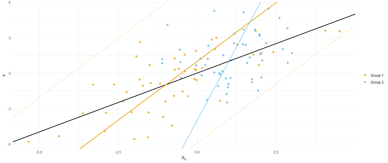
Thus, in Scenario 1, Separation does not seem to be a natural criterion for fairness because it suggests only counterproductive procedures for constructing estimators. However, we will show that in Scenario 2, Separation sometimes has the power to discriminate between subjectively different prediction rules.
4.1.3 Sufficiency
The Sufficiency criterion demands that whether an applicant will repay her loan is independent of her race conditional on the prediction . Because will always be a graphical descendent of some subset of the features, , , and , we can see from Figure 9 that we cannot achieve Sufficiency merely by carefully choosing ’s arguments. Conditioning on will never d-separate from .
However, we can see that the applicant’s credit rating d-separates from , and therefore any invertible function will satisfy Sufficiency. This argument will not generally work when the prediction rule is a function of more than one feature, though, since it is not generally possible to invert such a function. Indeed, in order to construct a prediction rule which satisfies Separation, the prediction must explicitly block the path between and . This can be done when the response only depends on the features and through a parameter : in this case, the predictor satisfies Sufficiency. Of course, the parameter which controls the way in which the probability of loan repayment depends on the loan interest rate and an applicant’s credit rating is not known in practice, so this exact predictor is not available for use. This argument further shows that, in this case, the only way that prediction rules which are estimated from training data can be Sufficient is through their recovery of the signal.
4.2 Scenario 2: Job Advertisement
In this scenario, modelled after a similar scenario from Barocas et al. 2018, we are looking to serve advertisements for a programming job to web users who are likely to be programmers. To predict whether or not the user is a programmer, we use information about his or her browsing history. For a real life example of issues in fairness which may arise from serving job advertisements, see Gillum and Tobin 2019. Suppose we model the relationship between measurements on an individual user using the PDAG in Figure 12.
|
We assume , a variable indicating whether a user has visited pinterest.com, has no relationship to whether or not the individual is a programmer except by virtue of the information it encodes about gender. The novelty of this scenario is that we observe , a variable indicating whether a user has visited stackexchange.com, which we assume is a graphical descendant of whether a user is a programmer, . According to this model, a user’s gender affects the likelihood that he or she is a programmer, but a programmer has a certain likelihood of visiting stackexchange.com regardless of his or her gender.
Therefore if we do not wish to target users for this employment advertisement based on gender, is a suspicious candidate, but may reasonably be considered fair game. We now examine the implications of the oblivious criteria in this scenario.
4.2.1 Independence
As in Scenario 1, if the prediction depends on whether a user has visited pinterest.com, , will violate Independence, and any information in which is independent of a user’s gender will also be independent of whether he or she is a programmer, . Furthermore, because is a descendant of with no backdoor connection to , any component of whether the user has visited stackexchange.com, , which is independent of will also be independent of . Therefore, we cannot construct any non-trivial predictions in Scenario 2 which satisfy Independence.
4.2.2 Separation
On the other hand, Scenario 2 is where Separation shines. Consider again estimators which depend on only one feature: let denote an arbitrary prediction rule which depends on only , and, likewise, let denote an arbitrary prediction rule which depends on only .
A prediction will fail to satisfy Separation because conditioning on whether a user is a programmer, , does not d-separate whether he or she has visited pinterest.com, , and his or her gender, . Clearly, this will be the case regardless of what information we extract from . However, any prediction which is a descendent only of whether the user has visited stackexchange.com, , will in fact satisfy Separation, because conditioning on blocks the path between and .
Thus we can interpret Separation as a criterion which encourages us to use information which depends on only through the response, . However, it is not clear that there are many situations in which we observe features which behave as graphical descendants of the response. We are generally interested in using features which temporally precede the observation of ; usually causes and not the other way around.
In fact Scenario 2, which was designed to illustrate a possible use of the Separation criterion, is unrealistic. A modification to Scenario 2 which is more realistic can be modelled with the PDAG in Figure 14.
|
Here, whether or not a user is a programmer is actually an unobserved variable, , and is relevant to us only because it determines the likelihood of the observable event that the user clicks on our advertisement, . From this more realistic model we can see that no longer d-separates from . Thus to the extent that is not identical to , Separation will not hold.
4.2.3 Sufficiency
In contrast to Scenario 1, we cannot construct a non-trivial prediction satisfying Sufficiency. Neither nor are mediators of the effect of on . The only way our prediction could block the direct path between and would be for to perfectly encode the information in .
5 Understanding Separation
Among the three oblivious criteria of fairness discussed, we are most skeptical of Separation. As mentioned in Section 3.2, there is a significant literature focused on applying and generalizing the criterion. However, unlike the other criteria, Separation has fundamental limitations, which we now explore.
In Section 4.2.2, we found that predictions which are a function of features that are descendants of the response will satisfy Separation, so we will now focus on other cases. In particular, we will focus on an arrangement of the features, sensitive characteristic, and response which we feel is most likely to occur in practice. We assume the DAG is arranged so that the sensitive characteristic is a root, the response is a leaf, and none of the features are descendants of the response. We feel that this DAG is ubiquitous since predictions are often made about the future, so that the features will need to be causal ancestors of the response. An example of such an arrangement is provided in Scenario 1. To be concrete, we will focus on a typical example of a DAG which encodes dependencies between the features, visualized in Figure 15.
We will let be a root node which may be an ancestor of any of the features, . Furthermore, features may be ancestors or descendants of each other, but all of the features are ancestors of the response, .
We will now argue that Separation will tend not to hold by examining the structure of the typical DAG, which is visualized with a prediction in the leftmost graph of Figure 17. There, conditioning on a leaf of the graph, the response , will not generally block paths from the root, the sensitive characteristic , to the prediction , which depends on the mediators, the features . This is due to a nondegeneracy of the graph: the response will be influenced by exogenous random noise, say , in addition to a signal through the features . Due to the interference of the noise , the information in the response is fundamentally different than the information in the features, which leads to the impossibility of blocking, and the failure of Separation.
This argument is easiest to see in the case of the visualized Figure 17, but holds more generally. Whenever there is at least one feature which is an ancestor of the response : the exogenous noise will still interfere with the response , leading to an inability to recover the information in the feature. Specializing the conclusion of this argument to the binary case uncovers a peculiarity in Equalized Odds, despite that Equalized Odds is derived from common measures for summarizing the accuracy of a classifier.
5.1 Incompatibility between Separation and Sufficiency
Measures of fairness were beginning to be intensely studied and debated when Kleinberg et al. 2017 and Chouldechova 2017 established the surprising result that Calibration and Equalized Odds cannot simultaneously hold in all but degenerate settings. Specifically, it was established:
Theorem 1.
Consider the binary setting, where the response and the prediction . When , the prediction can only satisfy both Equalized Odds and Calibration by Group if for all , i.e., the mean response does not differ between levels of the protected characteristic .
The theorem has been generalized beyond the binary case to hold for Separation and Sufficiency. Barocas et al. 2018 provide an argument using undirected graphs, which we now reproduce. In Theorem 1, we assumed that . In the general case, we similarly, but more generally, assume that all events in the joint distribution of have positive probability. This assumption makes it so that there’s no degeneracy between the random variables. Consider an undirected graphical model of the variables , and .
Separation requires that , so that there can be no edge between and . Similarly, Sufficiency requires that , so that there can be no edge between and . We indicate the impossibility of an edge with a dashed line. Therefore, it must hold that , since there can be no path drawn connecting and . This establishes the result: under the non-degeneracy assumption, if Separation and Sufficiency both hold, it must be that . The condition is a generalization of the condition in Theorem 1 that the mean response does not differ between levels of the protected characteristic .
These results cast the disagreement between ProPublica (Angwin et al. 2016) and Northpointe (Flores et al. 2016) in a new light. On one hand, the failure of the COMPAS algorithm to achieve equal error rates between groups does not seem to be an objective form of unfairness if it is mathematically impossible for a calibrated classifier to do so. On the other hand, there remains the question of whether disparate impact caused by unbalanced error rates is sufficient cause to dispense with calibration.
In binary classification settings, it is common to characterize the performance of a classifier using the false positive and false negative rate. These quantities specify the distribution of given . However, as we have seen using the example of a simple linear regression model in Section 4.1.2, attempting to enforce parity between quantities conditional on can lead to counterproductive procedures. Furthermore, as we have argued, even when Calibration by Group does not hold, in general there is no reason to expect conditioning on to block the paths between and . Thus we believe that the choice between Calibration by Group and Equalized Odds is not a mere subjective trade-off; instead we find Separation to be a fundamentally unhelpful fairness criterion.
5.2 Parity by Signal
The original motivation of Equalized Odds (Hardt et al. 2016) was to overcome limitations of Independence. In addition to the stringency of the criterion, the authors argue that a limitation of the criterion is that the response itself does not satisfy Independence whenever there is dependence between and the sensitive characteristic . This is undesirable, they write, since the response is an “ideal [prediction], which can hardly be considered discriminatory as it represents the actual outcome.”
This line of reasoning seems to obscure a crucial point. When the probability distribution of the response depends on the features only through a signal parameter , which we could take without loss of generality to be the conditional mean when is one-dimensional, the signal will not be an allowable prediction under Separation.
This follows by the same reasoning as in Section 5: in non-degenerate settings, conditioning on the response will not block the dependence between any of its ancestors. This is a significant limitation since the discrepancy between the response and the signal is generally unique to each individual and cannot be predicted. Indeed, no prediction rule can achieve zero prediction error when the response has an exogenous noise component. Therefore, in practicality, the perfect prediction is the signal , not the response . With this in mind, we explicitly define a new measure of fairness.
Definition 9.
Represent , where is exogenous noise, that is, , and is a function indexed by a signal parameter . Then a prediction satisfies Parity by Signal when is conditionally independent of the sensitive attribute given the signal , i.e. .
Another way to view this definition of fairness is that the predictions for similar people do not unnecessarily depend on the sensitive characteristic, where similar people are defined to be those whose features contribute—via the signal —in the same way to the outcome. This is related to the measure of fairness described by Dwork et al. 2012, wherein Separation by Signal would be considered as utilizing a perfect similarity metric. In Scenario 1, an optimal prediction rule which satisfies Separation was presented, and it was found to be unusual: however, in that same scenario, the true mean does indeed satisfy Parity by Signal.
This definition of fairness is not without its limitations. Evaluating whether a prediction satisfies Separation by Signal requires the signal , which is generally not known in practice. Above we demonstrated that Separation by Signal is a useful device to develop understanding, but a close variant of it can also be made operational. Separation by Signal compares the prediction to the signal , but, instead, could be compared to another prediction which we believe to be more accurate than .
Definition 10.
A prediction satisfies Parity by if is conditionally independent of the sensitive attribute given , i.e. .
Notice that a prediction satisfies Separation by Signal if and only if satisfies Separation by .
We can interpret a variety of fairness-testing procedures as a form of testing for Parity by . For example, in the context of testing whether various police precincts exhibit racial bias in contraband searches, Simoiu et al. 2017 develop a threshold test which is a test for a kind of Parity by Signal. They are in the binary setting and consider the prediction to be that an individual is carrying contraband when the probability of the individual carrying contraband is larger than a threshold and to be that an individual is not carrying contraband otherwise. They develop Bayesian tests for whether the threshold depends on the race , since they argue that a fundamental form of unfairness occurs when minorities are ruled against more stringent thresholds. Due to the prediction depending only on the probability and the threshold , this is a test for whether satisfies Parity by .
In the above example, the threshold test sought to determine whether there was a specific form of bias in police officers’ decisions to search for contraband. This is an example of testing subjective human predictions, with some modeling assumptions. However, a Separation by criterion can also be desirable to hold for a prediction even when both and are generated by machine algorithms. Consider cases in which we believe that a model is unfair due to misspecification; perhaps this model is missing necessary features or fails to model interactions between the sensitive characteristic and other features in a way which leads the predictions generated by the algorithm to disparately impact certain groups. (See in particular Scenario 1: The Red Car in Kusner et al. 2017.) Specifically, suppose that the prediction and the prediction , where each coefficient differs based on the sensitive characteristic . In this case, a likelihood ratio test (Agresti 2015) between these models would be a test for whether satisfies Separation by .
6 Causal Considerations
In various discussions of Independence and Separation-like criteria, authors propose generalizations which enforce parity only after conditioning on certain features (Barocas et al. 2018; Hardt et al. 2016; Donini et al. 2018). Consider the following generalizations of Independence. Suppose is some subvector of the features .
Definition 11.
A prediction satisfies Conditional Independence with respect to if .
Notice that Conditional Independence with respect to always holds when the prediction is a deterministic function of the features . This reinforces that the purpose of Conditional Independence is to study the influence of a subvector of the features. Notice also the connection to Parity by Signal and Parity by a prediction , discussed in Section 5.2, which involve evaluating independence conditional on a specific function of the features.
Conditional Independence criteria themselves convey little information about the underlying desires of the practitioner. However, causal reasoning can provide principled methods for developing fairness criteria which may ultimately be expressed as Conditional Independence criteria. Here, we discuss two scenarios in which Conditional Independence criteria can be derived using causal reasoning. For a variety of perspectives on the role of Pearl’s causality theory in fairness, see Kusner et al. 2017; Kilbertus et al. 2017; Nabi and Shpitser 2018 and Chiappa 2019.
6.1 Scenario 3: College Admissions
For the purpose of college admissions, we wish to predict whether a student will drop out before completing his or her degree. Suppose we model the situation using the PDAG in Figure 18.
|
Suppose that the admissions committee wishes to use all of the relevant information about student performance contained in the student’s SAT score , but otherwise wishes to ignore the student’s race-laden socioeconomic status , despite the fact that socioeconomic factors do have a direct effect on a student’s probability of dropping out. In the language of Kilbertus et al. 2017, this means that is a resolving variable. The Independence criterion would not allow us to use all of the information in , since we would have to extract the component of which is independent of the student’s race . Separation or Parity by Signal, on the other hand, would not allow us to fully make use of while entirely excluding information in .
In fact we actually desire for to have no direct effect on that is not mediated by . We can express this criterion using the formula for Controlled Direct Effect (CDE) as:
| (2) |
for all and all in the range of . In this case, this do-expression is identifiable and simplifies to the expression . However, in cases when a resolving variable is itself confounded with other variables, the do-expressions in (2) may be unidentifiable or require some do-calculus to resolve into observational expressions.
6.2 Scenario 4: Insurance Prices
In the scenarios we have discussed so far, we model the sensitive characteristic as an exogenous variable. Thus has always been a root in our PDAG models, and the total causal effects of on endogenous entities such as and coincide with the observed effects. However, when is an endogenous variable, there may be backdoor paths from to our predictions or response. Consider the following scenario, which makes clear the need for causal reasoning in fairness.
We wish to predict whether an individual is likely to have a car accident for the purpose of determining her insurance premium. Suppose we model the relevant variables using the PDAG in Figure 19.
|
We may deem it unfair to use an individual’s religion, , as a factor in our prediction, . However, there is a backdoor path between and , and thus and are marginally dependent. For the same reason, any prediction which is a non-trivial descendent of the individual’s driving record will fail to satisfy Independence. Of course, as in all of the ubiquitous cases when the features are ancestors of the response, conditioning on will not black the path between and either, thus our prediction will also fail to satisfy Separation.
In this case, we need not consider to be a resolving variable. Whatever dependence results between and is spurious. We are interested in ensuring that has no Total Effect (TE) on , which we can express as:
| (3) |
Note that this is a special case of the Counterfactual Fairness criterion in Kusner et al. 2017, although these authors do not explicitly consider cases in which is endogenous. The consequence of this criterion is that we can freely construct predictions which are based on traffic tickets, , or other inferred aspects of personality, .
7 Conclusion
In Scenarios 1 through 4, PDAGs have proven to be fertile ground for developing intuition about the three basic oblivious criteria for fairness: Independence, Separation, and Sufficiency. In general, constructing a PDAG model relating the sensitive characteristic, features, and response is a clarifying exercise, because it allows us to more directly connect our senses about what is intuitively fair to the implications of the decisions we make in specifying an algorithm. In contrast to the project of constructing statistically optimal estimators, a fundamental concern in constructing fair estimators is blocking the use of information which is subjectively unacceptable. Here, PDAGs and d-separation are natural tools.
In contrast, the oblivious fairness criteria alone are limited, because their behavior is opaque and sensitive to the particularities of the scenario. Enforcing Independence between the sensitive characteristic and the prediction was seen to have wildly different implications in scenarios when the response was dependent on race and when it was not. In the former case, Independence prohibited discrimination which could not be statistically justified, and in the latter case, Independence was an intervention in favor of adversely affected groups.
Sufficiency can be achieved by blocking all paths through which information can flow between the sensitive characteristic and the response. Generally this is only possible by accurately recovering the signal. That is, it was shown that Sufficiency can be achieved by appropriately choosing the features through which information flows from race to the response and appropriately choosing a prediction that blocks that flow of information.
Separation naturally allows for the use of features which are descendants of the response, but exhibits strange behavior whenever there are features which are non-descendants of the response, even when those features are independent of the sensitive characteristic. For non-degenerate and faithful PDAG models, Separation will not hold since the response is comprised of not only the signal, but also the noise, which obscures the information about the signal in the response. In Scenario 1, a violation of faithfulness was induced to produce an optimal prediction rule that turned out to be highly inappropriate, for some groups even requiring the addition of further random noise.
For the most part, these measures have been found wanting. We join the recent consensus that the assessment of fairness in algorithms should not start and end with the use of a singular criterion. The constraints we wish to impose on predictions should be sensitive to each scenario, and PDAG models can help to explore them.
More generally, we notice that there is little consensus on the underlying philosophical principles that should provide the foundation for the quantification of fairness. While much work in fairness seems to be framed around preventing unfairness like that allegedly exhibited by the COMPAS algorithm, there is no consensus that the COMPAS algorithm was ever unfair. We worry that as constructs from fairness are taken out of context and treated as black boxes for mathematical study and elaboration, the implicit underlying notions of fairness will be obscured. We hope that fairness research can be grounded in clear, practical examples of the ways algorithms can be unfair.
Acknowledgements
Thanks to David Kent for helpful conversations.
References
- Agresti (2015) Alan Agresti. Foundations of linear and generalized linear models. John Wiley & Sons, 2015.
- Ajunwa et al. (2016) Ifeoma Ajunwa, Sorelle Friedler, Carlos E Scheidegger, and Suresh Venkatasubramanian. Hiring by algorithm: predicting and preventing disparate impact. SSRN Electronic Journal, 2016.
- Angwin et al. (2016) Julia Angwin, Jeff Larson, Surya Mattu, and Lauren Kirchner. Machine bias: There’s software used across the country to predict future criminals. And it’s biased against blacks. ProPublica, 23, 2016.
- Barocas and Selbst (2016) Solon Barocas and Andrew D Selbst. Big data’s disparate impact. Calif. L. Rev., 104:671, 2016.
- Barocas et al. (2018) Solon Barocas, Moritz Hardt, and Arvind Narayanan. Fairness and Machine Learning. fairmlbook.org, 2018. http://www.fairmlbook.org.
- Binns (2017) Reuben Binns. Fairness in machine learning: Lessons from political philosophy. In Proceedings of Machine Learning Research, volume 81, 2017.
- Calders and Verwer (2010) Toon Calders and Sicco Verwer. Three naive bayes approaches for discrimination-free classification. Data Mining and Knowledge Discovery, 21(2):277–292, 2010.
- Calders et al. (2009) Toon Calders, Faisal Kamiran, and Mykola Pechenizkiy. Building classifiers with independency constraints. In 2009 IEEE International Conference on Data Mining Workshops, pages 13–18. IEEE, 2009.
- Chiappa (2019) Silvia Chiappa. Path-specific counterfactual fairness. In Thirty-Third AAAI Conference on Artificial Intelligence, 2019.
- Chouldechova (2017) Alexandra Chouldechova. Fair prediction with disparate impact: A study of bias in recidivism prediction instruments. Big data, 5(2):153–163, 2017.
- Chouldechova and Roth (2018) Alexandra Chouldechova and Aaron Roth. The frontiers of fairness in machine learning. arXiv:1810.08810, 2018.
- Corbett-Davies and Goel (2018) Sam Corbett-Davies and Sharad Goel. The measure and mismeasure of fairness: A critical review of fair machine learning. arXiv:1808.00023, 2018.
- Corbett-Davies et al. (2017) Sam Corbett-Davies, Emma Pierson, Avi Feller, Sharad Goel, and Aziz Huq. Algorithmic decision making and the cost of fairness. In Proceedings of the 23rd ACM SIGKDD International Conference on Knowledge Discovery and Data Mining, pages 797–806. ACM, 2017.
- Del Barrio et al. (2018) Eustasio Del Barrio, Fabrice Gamboa, Paula Gordaliza, and Jean-Michel Loubes. Obtaining fairness using optimal transport theory. arXiv:1806.03195, 2018.
- Donini et al. (2018) Michele Donini, Luca Oneto, Shai Ben-David, John S Shawe-Taylor, and Massimiliano Pontil. Empirical risk minimization under fairness constraints. In Advances in Neural Information Processing Systems, pages 2796–2806, 2018.
- Duffy (2016) Brooke Duffy. The romance of work: Gender and aspirational labour in the digital culture industries. International Journal of Cultural Studies, 19(4):441–457, 2016.
- Dwork et al. (2012) Cynthia Dwork, Moritz Hardt, Toniann Pitassi, Omer Reingold, and Richard Zemel. Fairness through awareness. In Proceedings of the 3rd innovations in theoretical computer science conference, pages 214–226. ACM, 2012.
- Eubanks (2018) Virginia Eubanks. Automating inequality: How high-tech tools profile, police, and punish the poor. St. Martin’s Press, 2018.
- Flores et al. (2016) Anthony W Flores, Kristin Bechtel, and Christopher T Lowenkamp. False positives, false negatives, and false analyses: A rejoinder to machine bias: There’s software used across the country to predict future criminals. and it’s biased against blacks. Fed. Probation, 80:38, 2016.
- Gillum and Tobin (2019) Jack Gillum and Ariana Tobin. Facebook won’t let employers, landlords or lenders discriminate in ads anymore. ProPublica, 2019.
- Grgic-Hlaca et al. (2016) Nina Grgic-Hlaca, Muhammad Bilal Zafar, Krishna P Gummadi, and Adrian Weller. The case for process fairness in learning: Feature selection for fair decision making. In NIPS Symposium on Machine Learning and the Law, volume 1, page 2, 2016.
- Hacker and Wiedemann (2017) Philipp Hacker and Emil Wiedemann. A continuous framework for fairness. arXiv:1712.07924, 2017.
- Hardt et al. (2016) Moritz Hardt, Eric Price, Nati Srebro, et al. Equality of opportunity in supervised learning. In Advances in neural information processing systems, pages 3315–3323, 2016.
- Johndrow and Lum (2019) James E Johndrow and Kristian Lum. An algorithm for removing sensitive information: application to race-independent recidivism prediction. The Annals of Applied Statistics, 13(1):189–220, 2019.
- Kilbertus et al. (2017) Niki Kilbertus, Mateo Rojas Carulla, Giambattista Parascandolo, Moritz Hardt, Dominik Janzing, and Bernhard Schölkopf. Avoiding discrimination through causal reasoning. In Advances in Neural Information Processing Systems, pages 656–666, 2017.
- Kleinberg et al. (2017) Jon Kleinberg, Sendhil Mullainathan, and Manish Raghavan. Inherent trade-offs in the fair determination of risk scores. In The 8th Innovations in Theoretical Computer Science Conference, 2017.
- Kusner et al. (2017) Matt J Kusner, Joshua Loftus, Chris Russell, and Ricardo Silva. Counterfactual fairness. In Advances in Neural Information Processing Systems, pages 4066–4076, 2017.
- Larson et al. (2016) Jeff Larson, Surya Mattu, Lauren Kirchner, and Julia Angwin. How we analyzed the compas recidivism algorithm. ProPublica, 9, 2016.
- Lichtenstein et al. (1981) Sarah Lichtenstein, Baruch Fischhoff, and Lawrence D Phillips. Calibration of probabilities: The state of the art to 1980. Technical report, Perceptronics: Decision Research, 1981.
- Lum (2017) Kristian Lum. Limitations of mitigating judicial bias with machine learning. Nature Human Behaviour, 2017.
- Mitchell et al. (2018) Shira Mitchell, Eric Potash, and Solon Barocas. Prediction-based decisions and fairness: A catalogue of choices, assumptions, and definitions. arXiv:1811.07867, 2018.
- Moser (1996) William R Moser. Linear models: A mean model approach. Elsevier, 1996.
- Nabi and Shpitser (2018) Razieh Nabi and Ilya Shpitser. Fair inference on outcomes. In Thirty-Second AAAI Conference on Artificial Intelligence, 2018.
- O’Neil (2017) Cathy O’Neil. Weapons of math destruction: How big data increases inequality and threatens democracy. Broadway Books, 2017.
- Pearl (2009a) Judea Pearl. Causal inference in statistics: An overview. Statistics surveys, 3:96–146, 2009a.
- Pearl (2009b) Judea Pearl. Causality. Cambridge University Press, 2009b.
- Pearl et al. (2016) Judea Pearl, Madelyn Glymour, and Nicholas P Jewell. Causal inference in statistics: A primer. John Wiley & Sons, 2016.
- Pleiss et al. (2017) Geoff Pleiss, Manish Raghavan, Felix Wu, Jon Kleinberg, and Kilian Q Weinberger. On fairness and calibration. In Advances in Neural Information Processing Systems, pages 5680–5689, 2017.
- Robinson and Yu (2014) Yu Robinson and H Yu. Knowing the score: New data, underwriting and marketing in the consumer credit marketplace. A Guide for Financial Inclusion Stakeholders, pages 1–34, 2014.
- Simoiu et al. (2017) Camelia Simoiu, Sam Corbett-Davies, Sharad Goel, et al. The problem of infra-marginality in outcome tests for discrimination. The Annals of Applied Statistics, 11(3):1193–1216, 2017.
- Spirtes et al. (2000) Peter Spirtes, Clark N Glymour, Richard Scheines, David Heckerman, Christopher Meek, Gregory Cooper, and Thomas Richardson. Causation, prediction, and search. MIT press, 2000.
- Stowe (2019) Stacy Stowe. New york city to ban discrimination based on hair. New York Times, 2019.
- Yeom and Tschantz (2018) Samuel Yeom and Michael Carl Tschantz. Discriminative but not discriminatory: A comparison of fairness definitions under different worldviews. arXiv:1808.08619, 2018.
- Zafar et al. (2017) Muhammad Bilal Zafar, Isabel Valera, Manuel Gomez Rodriguez, and Krishna P Gummadi. Fairness beyond disparate treatment & disparate impact: Learning classification without disparate mistreatment. In Proceedings of the 26th International Conference on World Wide Web, pages 1171–1180. International World Wide Web Conferences Steering Committee, 2017.
- Ziewitz (2016) Malte Ziewitz. Governing algorithms: Myth, mess, and methods. Science, Technology & Human Values, 41(1):3–16, 2016.