Morpheus: A Deep Learning Framework For Pixel-Level Analysis of Astronomical Image DataJournal: AAS Journals Python (Rossum 1995), NumPy (van der Walt et al. 2011), astropy (Price-Whelan et al. 2018), scikit-learn (Pedregosa et al. 2011), matplotlib (Hunter 2007), Docker (Merkel 2014), TensorFlow (Abadi et al. 2016)
Abstract
We present Morpheus, a new model for generating pixel-level morphological classifications of astronomical sources. Morpheus leverages advances in deep learning to perform source detection, source segmentation, and morphological classification pixel-by-pixel via a semantic segmentation algorithm adopted from the field of computer vision. By utilizing morphological information about the flux of real astronomical sources during object detection, Morpheus shows resiliency to false-positive identifications of sources. We evaluate Morpheus by performing source detection, source segmentation, morphological classification on the Hubble Space Telescope data in the five CANDELS fields with a focus on the GOODS South field, and demonstrate a high completeness in recovering known GOODS South 3D-HST sources with AB. We release the code publicly, provide online demonstrations, and present an interactive visualization of the Morpheus results in GOODS South.
I Introduction
Morphology represents the structural end state of the galaxy formation process. Since at least Hubble 1926, astronomers have connected the morphological character of galaxies to the physics governing their formation. Morphology can reflect the initial conditions of galaxy formation, dissipation, cosmic environment and large-scale tidal fields, merger and accretion history, internal dynamics, star formation, the influence of supermassive black holes, and a range of other physics (Binney 1978; Dressler 1980; Binney & Tremaine 1987; Djorgovski & Davis 1987; Dressler et al. 1987; Bender et al. 1992; Tremaine et al. 2002, e.g.,). The development of morphological measures for galaxies, therefore, comprises an important task in observational astronomy. To help realize the potential of current and future surveys for understanding galaxy formation through morphology, this work presents Morpheus, a deep learning-based model for the simultaneous detection and morphological classification of objects through the pixel-level semantic segmentation of large astronomical image datasets.
The established connections between morphology and the physics of galaxy formation run deep, and the way these connections manifest themselves observationally depends on the measures of morphology used. Galaxy size and surface brightness profile shape have served as common proxies for morphology, as quantitatively measured from the light distribution of objects (Vaucouleurs 1959; Sersic 1968; Peng et al. 2010). Size, radial profile, and isophotal shape or ellipticity vary with stellar mass and luminosity (Kormendy 1977; Roberts & Haynes 1994; Shen et al. 2003; Sheth et al. 2010; Bruce et al. 2012; van der Wel et al. 2012; van der Wel et al. 2014; Morishita et al. 2014; Huertas-Company et al. 2015; Allen et al. 2017; Jiang et al. 2018; Miller et al. 2019; Zhang et al. 2019, e.g.,). When controlled for other variables, these measures of galaxy morphology may show variations with cosmic environment (Dressler et al. 1997; Smail et al. 1997; Cooper et al. 2012; Huertas-Company et al. 2016; Kawinwanichakij et al. 2017), redshift (Abraham & van den Bergh 2001; Trujillo et al. 2004; Conselice et al. 2005; Elmegreen et al. 2005; Trujillo et al. 2006; Lotz et al. 2008; van Dokkum et al. 2010; Patel et al. 2013; Shibuya et al. 2015), color (Franx et al. 2008; Yano et al. 2016), star formation rate or quiescence (Toft et al. 2007; Zirm et al. 2007; Wuyts et al. 2011; Bell et al. 2012; Lee et al. 2013; Whitaker et al. 2015), internal dynamics (Bezanson et al. 2013), the presence of active galactic nuclei (Kocevski et al. 2012; Bruce et al. 2016; Powell et al. 2017), and stellar age (Williams et al. 2017). The presence and size of bulge, disk, and bar components also vary with mass and redshift (Sheth et al. 2008; Simmons et al. 2014; Margalef-Bentabol et al. 2016; Dimauro et al. 2018), and provide information about the merger rate (Lofthouse et al. 2017; Weigel et al. 2017, e.g.,). Galaxy morphology encodes a rich spectrum of physical processes and can augment what we learn from other galaxy properties.
While complex galaxy morphologies may be easily summarized with qualitative descriptions (e.g., “disky”, “spheroidal”, “irregular”), providing quantitative descriptions of this complexity represents a long-standing goal for the field of galaxy formation and has motivated ingenuitive analysis methods including measures of galaxy asymmetry, concentration, flux distribution (Abraham et al. 1994; Abraham et al. 1996; Conselice et al. 2000; Conselice 2003; Lotz et al. 2004, e.g.,), shapelet decompositions (Kelly & McKay 2004; Kelly & McKay 2005), morphological principal component analyses (Peth et al. 2016), and unsupervised morphological hierarchical classifications (Hocking et al. 2018). These measures provide well-defined characterizations of the surface brightness distribution of galaxies and can be connected to their underlying physical state by, e.g., calibration through numerical simulation (Huertas-Company et al. 2018). The complementarity between these quantitative measures and qualitative morphological descriptions of galaxies means that developing both classes of characterizations further can continue to improve our knowledge of galaxy formation physics.
Characterizing large numbers of galaxies with descriptive classifications simultaneously requires domain knowledge of galaxy morphology (“expertise”), the capability to evaluate quickly each galaxy (“efficiency”), a capacity to work on significant galaxy populations (“scalability”), some analysis of the data to identify galaxy candidates for classification (“pre-processing”), a presentation of galaxy images in a format that enables the characteristic structures to be recognized (“data model”), and an output production of reliable classifications (“accuracy”). Methods for the descriptive classification of galaxy morphology have addressed these challenges in complementary ways.
Perhaps the most important and influential framework for galaxy morphological classification to date has been the Galaxy Zoo project (Lintott et al. 2008; Willett et al. 2013; Willett et al. 2017), which enrolls the public in the analysis of astronomical data including morphological classification. This project has addressed the expertise challenge by training users in the classification of galaxies and statistically accounting for the distribution of users’ accuracies. The efficiency of users varies, but by leveraging the power of the public interest and enthusiasm, and now machine learning (Beck et al. 2018; Walmsley et al. 2019), the project can use scalability to offset variability in the performance of individual users. The pre-processing and delivery of suitable images to the users has required significant investment and programming, but has led to a robust data model for both the astronomical data and the data provided by user input. Science applications of Galaxy Zoo include quantitative morphological descriptions of 50,000 galaxies (Simmons et al. 2017) in the CANDELS survey (Grogin et al. 2011; Koekemoer et al. 2011), probes of the connection between star formation rate and morphology in spiral galaxies (Willett et al. 2015), and measuring galaxy merger rates (Weigel et al. 2017).
Other efforts have emphasized different dimensions of the morphological classification task. Kartaltepe et al. 2015 organized the visual classification of 10,000 galaxies in CANDELS by a team of dozens of professional astronomers. This important effort performed object detection and source extraction on the CANDELS science data, assessed their completeness, and provided detailed segmentation maps of the regions corresponding to classified objects. The use of high expertise human classifiers leads to high accuracy, but poses a challenge for scalability to larger samples. The work of Kartaltepe et al. 2015 also leveraged a significant investment in the preprocessing and presentation of the data to their users with a custom interface with a high-quality data model for the results.
Leveraging human classifiers, be they highly expert teams or well-calibrated legions, to provide descriptive morphologies for forthcoming datasets will prove challenging. These challenges motivate a consideration of other approaches, and we present two salient examples in James Webb Space Telescope (Gardner et al. 2006, JWST;) and the Large Synoptic Survey Telescope (Ivezić et al. 2019; LSST Science Collaboration et al. 2009, LSST;).
JWST enables both sensitive infrared imaging with NIRCam and multiobject spectroscopy with NIRSpec free of atmospheric attenuation. The galaxy population discovered by JWST will show a rich range of morphologies, star formation histories, stellar masses, and angular sizes (Williams et al. 2018), which makes identifying NIRCam-selected samples for spectroscopic follow-up with NIRSpec challenging. The efficiency gain of parallel observations with NIRCam and NIRSpec will lead to programs where the timescale for constructing NIRCam-selected samples will be very short (2 months) to enable well-designed parallel survey geometries. For this application, the ability to generate quick morphological classifications for thousands of candidate sources will enhance the spectroscopic target selection in valuable space-based observations.
LSST presents a challenge of scale, with an estimated 30 billion astronomical sources, including billions of galaxies over 17,000 (LSST Science Collaboration et al. 2009). The morphological classification of these galaxies will require the development of significant analysis methods that can both scale to the enormity of the LSST dataset and perform well enough to allow imaging data to be reprocessed in pace with the LSST data releases. Indeed, morphological classification methods have been identified as keystone preparatory science tasks by in the LSST Galaxies Science Roadmap (Robertson et al. 2017, see also Robertson et al. 2019.).
Recently, advances in the field of machine learning called deep learning have enjoyed success in morphological classification. Dieleman et al. 2015 (D15) and Dai & Tong 2018 use deep learning to classify the Galaxy Zoo Survey. Huertas-Company et al. 2015 used a deep learning model derived from D15 and the classifications from K15 to classify the CANDELS survey. González et al. 2018 used deep learning to perform galaxy detection and morphological classification, an approach that has also been used to characterize Dark Energy Survey galaxy morphologies (Tarsitano et al. 2018). Deep learning models have been further applied to infer the surface brightness profiles of galaxies (Tuccillo et al. 2018) and measure their fluxes (Boucaud et al. 2019), and now to simulate entire surveys (Smith & Geach 2019).
Here, we extend previous efforts by applying a semantic segmentation algorithm to both classify pixels and identify objects in astronomical images using our deep learning framework called Morpheus. The software architecture of the Morpheus framework is described in Section II, with the essential convolutional neural network and deep learning components reviewed in Appendix A. The Morpheus framework has been engineered by using TensorFlow (Abadi et al. 2016) implementations of these components to perform convolutions and tensorial operations, and is not a port of existing deep learning frameworks or generated via “transfer learning”(Pratt 1993, e.g.,) of existing frameworks pre-trained on non-astronomical data such as ImageNet (Deng et al. 2009).
We train Morpheus using multiband Flexible Image Transport System (Wells et al. 1981, FITS;) images of CANDELS galaxies visually classified by Kartaltepe et al. 2015 and their segmentation maps derived from standard sextractor analyses (Bertin & Arnouts 1996). The training procedure is described in Section III, including the “loss function” used to optimize the Morpheus framework. Since Morpheus provides local estimates of whether image pixels contain source flux, the Morpheus output can be used to perform source segmentation and deblending. We present fiducial segmentation and deblending algorithms for Morpheus in Section IV.
We then apply Morpheus to the Hubble Legacy Fields (Illingworth et al. 2016) reduction of the CANDELS and GOODS data in the GOODS South region, the v1.0 data release (Grogin et al. 2011; Koekemoer et al. 2011) for the other four CANDELS regions, and generate FITS data files of the same pixel format as the input FITS images, each containing the pixel-by-pixel model classifications of the image data into spheroid, disk, irregular, point source/compact, and background classes, as described in Section VI. We release publicly these Morpheus pixel-level classification data products and detailed them in Appendix D. We evaluate the performance of Morpheus in Section VII, including tests that use the catalog of 3D-HST photometric sources (Skelton et al. 2014; Momcheva et al. 2016) to measure the completeness of Morpheus in recovering sources as a function of source magnitude. We find that Morpheus is highly complete () for sources up to one magnitude fainter than objects used to train the model. Using the Morpheus results, we provide estimates of the morphological classification of 3D-HST sources as a public value-added catalog, described in Section VIII. In Section IX, we discuss applications of Morpheus and semantic segmentation, which extend well beyond morphological classification, and connect the capabilities of Morpheus to other research areas in astronomical data analysis. We publicly release the Morpheus code, provide on-line tutorials for using the framework via Jupyter notebooks, and present an interactive website to visualize the Morpheus classifications and segmentation maps in the context of the HLF images and 3D-HST catalog. These software and data releases are described in Appendices B, C, and D. A summary of our work is presented with some conclusions in Section X. Throughout the paper, we have used the AB magnitude system (Oke & Gunn 1983) and assumed a flat CDM universe (, ) with a Hubble parameter km/s/Mpc when necessary.
II Morpheus Deep Learning Framework
Morpheus provides a deep learning framework for analyzing astronomical images at the pixel level. Using a semantic segmentation algorithm, Morpheus identifies which pixels in an image are likely to contain source flux and separates them from “background” or sky pixels. Morpheus, therefore, allows for the definition of corresponding segmentation regions or “segmentation maps” by finding contiguous regions of source pixels distinct from the sky. Within the same framework, Morpheus enables for further classification of the source pixels into additional “classes”. In this paper, we have trained Morpheus to classify the source pixels into morphological categories (spheroid, disk, irregular, point source/compact, and background) approximating the visual classifications performed by the CANDELS collaboration in K15. These source pixel classes identified by Morpheus could, in principle, be trained to reproduce other properties of the galaxies, such as, e.g., photometric redshift, provided a sufficient training dataset is available. In the sections below, we describe the architecture of the Morpheus deep learning framework. Readers unfamiliar with the primary computational elements of deep learning architectures may refer to Appendix A where more details are provided.
II.1 Input Data
We engineered the Morpheus deep learning framework to accept astronomical image data as direct input for pixel-level analysis. Morpheus operates on science-quality FITS images, with sufficient pipeline processing (e.g., flat fielding, background subtraction, etc.) to enable photometric analysis. Morpheus accepts multiband imaging data, with a FITS file for each of the bands used to train the model (see Section III). The pixel format of the input FITS images (or image region) matches the format of FITS images used to perform training, reflecting the size of the convolutional layers of the neural network determined before training. Morpheus allows for arbitrarily large images to be analyzed by subdividing them into regions that the model processes in parallel, as described in Section II.3 below.
For the example application of morphological classification presented in this paper, we use the (), (), (), and () band images from Hubble Space Telescope for training, testing, and our final analysis. Our training and testing images were FITS thumbnails and segmentation maps provided by Kartaltepe et al. 2015. Once trained, Morpheus can be applied to arbitrarily large images via a parallelization scheme described below in Section II.3. We have used the CANDELS public release data (Grogin et al. 2011; Koekemoer et al. 2011) in additional performance tests and the Hubble Legacy Fields v2.0 data (Illingworth et al. 2016) for our Morpheus data release.
We note that the approach taken by Morpheus differs from deep learning models that use traditional image formats, e.g., three-color Portable Network Graphics (PNG) or Joint Photographic Experts Group (JPEG) images as input. Using PNG or JPEG files as input is convenient because deep learning models trained on existing PNG or JPEG datasets, such as ImageNet (Deng et al. 2009; Russakovsky et al. 2015), can be retrained via transfer learning to classify galaxies. However, the use of these inputs requires additional pre-processing beyond the science pipeline, including arbitrary decisions about how to weight the FITS images to represent the channels of the multicolor PNG or JPEG. With the goal of including Morpheus framework analyses as part of astronomical pipelines, we have instead used FITS images directly as input to the neural network.
II.2 Neural Network
Morpheus uses a neural network inspired by the U-Net architecture (Ronneberger et al. 2015, See Section A.5) and is implemented using Python 3 (Rossum 1995) and the TensorFlow library (Abadi et al. 2016). We construct Morpheus from a series of “blocks” that combine multiple operations used repeatedly by the model. Each block performs a sequence of “block operations”. Figure 1 provides an illustration of a Morpheus block and its block operations. Block operations are parameterized by the number of convolved output images, or “feature maps”, they produce, one for each convolutional artificial neuron in the layer. We describe this process in more detail below.
Consider input data , consisting of layers of images with pixels. We define a block operation on as
| (1) |
where ReLU is the Rectified Linear Unit activation function (ReLU; Hahnloser et al. 2000; Lecun et al. 2015, See also Appendix A.1), is a convolutional layer (see Appendix A.3) with a number convolutional artificial neurons (see Appendix A.3), and BN is the batch normalization procedure (Ioffe & Szegedy 2015, and Appendix A.4.4). Note that the values of appearing in and are equal. For example, would indicate that the convolutional layer within the function has 4 convolutional artificial neurons. Unless stated otherwise, all inputs into a convolutional layer are zero-padded to preserve the width and height of the input, and all convolutional artificial neurons have kernel dimensions . Given Equation 1, for an input with dimensions the output of the function would have dimensions .
Equation 1 allows for a recursive definition of a function describing a series of block operations, where the input data to one block operation consist of the output from a previous block operation. This recursion can be written as
| (2) |
Equation 2 introduces a new parameter , shown with a superscript in . The parameter establishes the conditions of a base case for the recursion. Note that in Equation 2 the input is processed directly when , and when the input to the function is the output from . It can be seen from the formulation of Equations 1 and 2 that .
Since a block performs a number block operations, we can define a block mathematically as
| (3) |
An example block and its block operations can be seen diagrammatically in Figure 1. With these definitions, we can present the neural network architecture used in Morpheus.
Like the U-Net architecture, the Morpheus architecture consists of a contraction phase and an expansion phase. The contraction phase consists of three blocks with parameters , , and . Each block is followed by a max-pooling operation with size=() (see Section A.4.1), halving the width and height of its input. After the contraction phase there is a single intermediary block preceding the expansion phase with the parameters . The expansion phase consists of three blocks with the parameters , , . Each block is preceded by a bicubic interpolation operation that doubles the width and the height of its input. Importantly, the output from each block in the contraction phase is concatenated (see Section A.4.3) with the output from the bicubic interpolation operation in the expansion phase whose output matches its width and height (see Figure 2). The output from the final block in the expansion phase is passed through a single convolutional layer with 5 convolutional artificial neurons. A softmax operation (see Equation 4) is performed on the values in each pixel, ensuring the values sum to unity. The final output is a matrix with the same width and height as the input into the network, but where the last dimension, 5, now represents a classification distribution describing the confidence the corresponding pixel from the input belongs to one of the 5 specified morphological classes.
The blocks in Morpheus are organized into the U-Net structure, shown in Figure 2. The model proceeds clockwise, starting from “Input” on the upper left through to “Output” on the lower left. The very first step involves the insertion of the input FITS images into the model. Each FITS image is normalized to have a mean of 0 and unit variance before processing by Morpheus. We will refer to the number of input bands as , and in the application presented here, we take (i.e., ). The input images each have pixel dimensions , and we can, therefore, consider the astronomical input data to have dimensions . Only the first block operation takes the FITS images as input, and every subsequent block operation in the model takes the output from previous blocks as input.
The first convolution in the first block operation convolves the normalized astronomical data with three-dimensional kernels of size , and each element of the kernel is a variable parameter of the model to be optimized. The convolutions operate only in the two pixel dimensions, such that convolutions are performed, one for each pixel image, using a different kernel for each convolution. The convolved images are then summed pixel by pixel to create an output feature map of size . The convolutional layer repeats this process times with different kernels, generating output feature maps and an output dataset of size . For the first block in Morpheus we use (see Figure 2). After the first convolution on the astronomical data, every subsequent convolution in the first block has both input and output data of size .
Each block performs a number block operations, resulting in output data with dimensions of emerging from the block. The number of feature maps changes with each block. For a block producing filters, if the data incoming into the block has size with , then the first convolutional layer in the first block operation will have kernels of size . All subsequent convolutional layers in the block will then ingest and produce data of size by using kernels of size .
We can apply further operations on the data in between the blocks, and the character of these operations can affect the dimensions of the data. The first half of the model is a contraction phase, where each block is followed by a max-pooling operation (Cireşan et al. 2012, and Appendix A.4.1). The max-pooling is applied to each feature map output by the block, taking the local maximum over small areas within each feature map (in the version of Morpheus presented here, a pixel region) and reducing the size of the data input to the next block by the same factor. For this paper, the contraction phase in the Morpheus framework uses three pairs of blocks plus max-pooling layers.
After the contraction phase, the model uses a series of blocks, bicubic interpolation layers, and data concatenations in an expansion phase to grow the data back to the original format. Following each block in the expansion phase, a bicubic interpolation layer expands the feature maps by the same areal factor as the max-pooling layers applied in the contraction phase ( in the version of Morpheus presented here). The output feature maps from the interpolation layers are concatenated with the output feature maps from the contraction phase blocks where the data have the same format. Finally, the output from the last block in the expansion phase is input into a convolutional layer that produces the final output images that we call “Morpheus classification images”, one image for each class. The pixel values in these images contain the model estimates for their classification, normalized such that the element-wise sum of the classification images equals unity. For this paper, where we are performing galaxy morphological classification, there are five classification images (spheroid, disk, irregular, point source /compact, and background).
As the data progresses through the model, the number of feature maps and their shapes change owing to the max-pooling and interpolation layers. For reference, in Table 1, we list the dimensions of the data at each stage in the model, assuming input images in bands, each with pixels, and a total of classification images produced by the model.

| Layer | Input | Output Dimensions |
|---|---|---|
| Input Images | Bands, Pixels | [, , ] |
| Block 1a | Input Images | [, , 8] |
| Block 1b | Block 1a | [, , 8] |
| Block 1c | Block 1b | [, , 8] |
| Block 1d | Block 1c | [, , 8] |
| Max Pooling 1 | Block 1d | [, , 8] |
| Block 2a | Max Pooling 1 | [, , 16] |
| Block 2b | Block 2a | [, , 16] |
| Block 2c | Block 2b | [, , 16] |
| Block 2d | Block 2c | [, , 16] |
| Max Pooling 2 | Block 2d | [, , 16] |
| Block 3a | Max Pooling 2 | [, , 32] |
| Block 3b | Block 3a | [, , 32] |
| Block 3c | Block 3b | [, , 32] |
| Block 3d | Block 3c | [, , 32] |
| Max Pooling 3 | Block 3d | [, , 32] |
| Block 4a | Max Pooling 3 | [, , 16] |
| Interpolation 1 | Block 4a | [, , 16] |
| Block 5a | Interp. 1 + Block 3d | [, , 8] |
| Block 5b | Block 5a | [, , 8] |
| Interpolation 2 | Block 5b | [, , 8] |
| Block 6a | Interp. 2 + Block 2d | [, , 16] |
| Block 6b | Block 6a | [, , 16] |
| Interpolation 3 | Block 6b | [, , 16] |
| Block 7a | Interp. 3 + Block 1d | [, , 32] |
| Block 7b | Block 7a | [, , 32] |
| Convolution | Block 7b | [, , ] |
II.3 Parallelization for Large Images
While the Morpheus neural network performs semantic segmentation on pixels in FITS images with a size determined by the training images, the model can process and classify pixels in arbitrarily large images. To process large images, Morpheus uses a sliding window strategy by breaking the input FITS files into thumbnails of size (the size of the training images) and classifying them individually. Morpheus proceeds through the large format image, first column by column, and then row by row, shifting the active window by a unit pixel stride and then recomputing the classification for each pixel.
As the classification process continues with unit pixel shifts, each pixel is deliberately classified many times. We noticed heuristically that the output Morpheus classification of pixels depended on their location within the image, and that the pixel classifications were more accurate relative to our training data when they resided in the inner region of the classification area, where the lesser accuracy region consisted of a border about pixels wide on each side. Outside of the very outer pixels in the large format image, Morpheus classifies each pixel times. For the large FITS data images used in this paper, this repetition corresponds to separate classifications per pixel per output class, where each classification occurs when the pixel lies at a different location within the active window. This substantial additional information can be leveraged to improve the model, but storing the full “distribution” of classifications produced by this method would increase our data volume by roughly three orders of magnitude.
While Morpheus would enable full use of these distributions, for practical considerations, we instead record some statistical information as the computation proceeds and do not store the entire set of samples. To avoid storing the full distribution, we track running estimates of the mean and variance of the distribution11 1 See, e.g., http://people.ds.cam.ac.uk/fanf2/hermes/doc/antiforgery/stats.pdf for an example of running mean and variance estimators.. Once the mean for each class for each pixel is computed, we normalize the means across classes to sum to unity. We further record a statistic we call rank voting, which is a tally of the number of times each output class was computed by the model to be the top class for each pixel. The sum of rank votes across classes for a single pixel equals the number of times Morpheus processed the pixels (i.e., for most pixels). After the computation, the rank votes are normalized to sum to unity across the classes for each pixel.
The strips of classified regions produce fifteen output images, containing the mean and variance estimators for the classification distribution and normalized rank votes for each class. This striped processing of the image can be performed in parallel across multiple Morpheus instances and then stitched back together. The weak scaling of this processing is, in principle, trivial and is limited only by the number of available GPUs and the total memory of the computer used to perform the calculation.
III Model Training
The training of deep learning frameworks involves important decisions about the training data, the metrics used to optimize the network, numerical parameters of the model, and the length of training. We provide some rationale for these choices below.
III.1 Training Data
To train a model to perform semantic segmentation, we require a dataset that provides both information on the segmentation of regions of interest and classifications associated with those regions. For galaxy morphological classification, we use 7,629 galaxies sampled from the K15 dataset. Their 2-epoch CANDELS data provide an excellent combination of multiband FITS thumbnails, segmentation maps in FITS format, and visually-classified morphologies in tabulated form. The K15 classifications consisted of votes by expert astronomers, between per object, who inspected images of galaxies and then selected from several morphological categories to assign to the object. The number of votes for each category for each object are provided, allowing Morpheus to use the distribution of votes across classifications for each object when training. We downloaded and used the publicly available K15 thumbnail FITS files for the , , , and bands as input into the model for training and testing. In training Morpheus to reproduce the K15 classifications, multiband data approximates the information provided to the astronomers who performed the K15 classifications. Morpheus is trained using the same , , , and -band image thumbnails used in the K15 classification process. Other bands or different numbers of bands could be used for training as necessary, and Morpheus allows for reconfiguration and retraining depending on the available training images. Of the K15 data set, we used of the objects to form our training sample and to form our test sample. Various statistical properties of the test and training samples are described throughout the rest of the paper.
The primary K15 classifications spheroid, disk, irregular, and point source/compact were used in the example Morpheus application presented here. We added one additional class, background, to represent sky pixels absent significant source flux. We classify pixels as belonging to the background category if those pixels fell outside the K15 segmentation maps. Pixels inside the segmentation maps were assigned the distribution of classifications provided by the K15 experts.
The K15 classification scheme also included an unknown class for objects. Since Morpheus works at the pixel level and could provide individual pixel classifications that were locally accurate within a source but that collectively could sum to an object whose morphology expert astronomers might classify as unknown, we were posed with the challenge of how to treat the K15 unknown class. Given our addition of the background class constructed from large image regions dominated by sky, one might expect overlap in the features of regions that are mostly noise and amorphous regions classified as unknown. Since one might also expect overlap between unknown and irregular classifications, we wanted to preserve some distinction in the object classes. We, therefore, removed the unknown class by removing any sources that had unknown as their primary classification from the training sample (213 sources). For any sources where the non-dominant K15 classifications included unknown, we redistributed the unknown votes proportionally to the other classes.
III.2 Data Augmentation
To increase the effective size of the training dataset, Morpheus uses a data augmentation method. Augmentation supplements the input training data set by performing transformations on the training images to alter them with the intent of adding similar but not identical images with known classifications. Augmentation has been used successfully in the context of galaxy morphological classification (Dieleman et al. 2015, e.g.,), and Morpheus adopts a comparable approach to previous implementations.
During training, Morpheus produces a series of pixel augmented versions of the training images. The augmentation approach is illustrated in Figure 3. For each band in the original training image, the image is collectively rotated by a random angle , flipped horizontally with a random probability, and then flipped vertically with a random probability. A crop of the inner pixels of the resulting image is produced, and then a random pixel subset of the image is selected and passed to the model for training. This method allows us to increase the effective number of images available for training by a factor of and helps ameliorate over-training on the original training image set.

III.3 Loss Function
A standard method for training deep learning frameworks is to define a loss function that provides a statistic based on the output classifications to optimize via stochastic gradient descent with gradients computed using back-propagation (Rumelhart et al. 1986). Here, we describe how the Morpheus loss function is constructed.
The first task is to assign a distribution of input classifications on a per-pixel basis, choosing between the classes available to the Morpheus model. For this work, we choose (background, disk, spheroid, irregular, and point source/compact), but Morpheus can adopt an arbitrary number of classes. We use the index to indicate a given class, with . Consider an image of an astronomical object that has been visually classified by a collection of experts, and a segmentation map defining the extent of the object in the image. Outside the segmentation map of the object, the pixels are assumed to belong to the sky and are assigned the background class. Inside the segmentation map, pixels are assigned the distribution of disk, spheroid, irregular, and point source/compact classifications determined by the experts for the entire object. For each pixel , with rows and columns, we then have the vector whose elements contain the input distribution of classifications. Here, the index runs over the number of classes and for each pixel with indices . The goal of the model is to reproduce this normalized distribution of discrete classes for each pixel of the training images. We wish to define a total loss function that provides a single per-image statistic for the model to optimize when attempting to reproduce . Morpheus combines a weighted cross entropy loss function with a Dice loss (Novikov et al. 2017; Milletari et al. 2016) for its optimization statistic, which we describe below.
At the end of the Morpheus data flow, as outlined in Figure 2, the raw output of the model consists of vectors with elements per-pixel estimates that represent unnormalized approximations to the input per-pixel distributions . The model outputs for each pixel are then normalized to form a probability distribution using the softmax function
| (4) |
The distribution then represents the pixel-by-pixel classifications computed by Morpheus for each of the classes. For a pixel with indices , we can define the per-pixel cross entropy loss function as
| (5) |
where and are again the two per-pixel probability distributions, with representing the true distribution of the input classifications for the pixel and representing the model output.
Equation 5 provides the per-pixel contribution to the entropy loss function. However, for many images, the majority of pixels lie outside the segmentation maps of sources identified in the training data and are therefore labeled as background. To overcome this imbalance and disincentivize the model from erroneously learning to classify pixels containing source flux as background, we apply a weighting to the per-pixel loss. We define an index that indicates which class is the maximum of the input classification distribution for each pixel, written as
| (6) |
with . For each class , we then define a weight that is inversely proportional to the number of pixels with . We can write
| (7) |
Here, is the Kronecker delta function. The vector has size and each of its elements contain the inverse of the sum of for pixels with . In a given image, we ignore any classes that do not appear in the input classification distribution (i.e., any class for which ).
Using , we define a weighted cross entropy loss for each pixel as
| (8) |
A mean weighted loss function is then computed by averaging Equation 8 over all pixels as
| (9) |
This mean weighted loss function serves as a summary statistic of the cross entropy between the output of Morpheus and the input classification distribution.
When segmenting images primarily comprised of background pixels, the classification distributions of the output pixels should be highly unbalanced, with the majority having background. In this case, the mean loss function statistic defined by Equation 9 will be strongly influenced by a single class. A common approach to handle unbalanced segmentations is to employ a Dice loss function to supplement the entropy loss function (Milletari et al. 2016; Sudre et al. 2017, e.g.,). The Dice loss function used by Morpheus is written as
| (10) |
Here, is the sigmoid function (see Equation A3) applied pixel-wise to the background classification image output by the model. The image is the input mask with values denoting background pixels and indicating source pixels, defined, e.g., by a segmentation map generated using sextractor. The symbol indicates a Hadamard product of the matrices and . Note that the output background matrix has not yet been normalized using a softmax function, and so and . The Dice loss then ranges from if and when and differ substantially. The addition of this loss function helps to maximize the spatial coincidence of the output background pixels assigned with the non-zero elements of the input segmentation mask .
To define the total loss function optimized during the training of Morpheus, the cross entropy and Dice losses are combined as a sum weighted by two parameters and . The total loss function is written as
| (11) |
For the implementation of Morpheus used in this paper, the entropy and Dice loss functions are weighted equally by setting and .
III.4 Optimization Method
To optimize the model parameters, the Adam stochastic gradient descent method (Kingma & Ba 2014) was used. The Adam algorithm uses the first and second moments of first-order gradients computed via backpropagation to find the minimum of a stochastic function (in this case, our loss function, see Section III.3, which depends on the many parameters of the neural network). The Adam optimizer, in turn, depends on hyper-parameters that determine how the algorithm iteratively finds a minimum. Since the loss function is stochastic, the gradients change each iteration, and Adam uses an exponential moving average of the gradients () and squared gradients () when searching for a minimum. Two dimensionless hyper-parameters ( and ) set the decay rates of these exponential averages (Kingma & Ba 2014, see Algorithm 1 of ). As the parameters of the function being optimized are iterated between steps and , they are updated according to
| (12) |
Here, is a small, dimensionless safety hyper-parameter that prevents division by zero, and is a small, dimensionless hyper-parameter that determines the magnitude of the iteration step. Table 2 lists the numerical values of the Adam optimizer hyper-parameters used by Morpheus. We use the default suggested values for , , and . After some experimentation, we adopted a more conservative step size for than used by Kingma & Ba 2014.
| Adam Optimizer Hyper-parameters | |
|---|---|
| Hyper-parameter | Value |
III.5 Model Evaluation
| Morpheus Training and Test Results | ||
|---|---|---|
| Metric | Training | Test |
| Accuracy | ||
| Background | 91.5% | 91.4% |
| Disk | 74.9% | 75.1% |
| Irregular | 80.6% | 68.6% |
| Point source/compact | 91.0% | 83.8% |
| Spheroid | 72.3% | 71.4% |
| All Classes | 86.8% | 85.7% |
| Intersection-Over-Union | ||
| 0.899 | 0.888 | |
| 0.900 | 0.891 | |
| 0.902 | 0.893 | |
| 0.902 | 0.895 | |
| 0.900 | 0.896 | |
As training proceeds, the performance of the model can be quantified using various metrics and monitored to determine when training has effectively completed. The actual performance of Morpheus will vary depending on the classification scheme used, and here we report the performance of the model relative to the CANDELS images morphologically classified in K15. Performance metrics reported in this Section refer to pixel-level quantities, and we discuss object-level comparisons of morphological classifications relative to K15 in Section V.
While the model training proceeds by optimizing the loss function defined in Section III.3, we want to quantify the accuracy of the model in recovering the per-pixel classification and the overlap of contiguous regions with the same classification. First, we will need to define the index with maximum probability to reflect either the input classification or the output classification . We define an equivalent of Equation 6 for as
| (13) |
We can then define a percentage accuracy
| (14) |
The accuracy then provides the percentage of pixels for which the maximum probability classes of the input and output distributions match.
In addition to accuracy, the intersection-over-union of pixels with background probabilities above some threshold is computed between the input and output distributions. If we define the index to represent the background class, we can express the input background probabilities as for and , and the equivalent for the output background probabilities . We can refer to and as the input and output background images, and the regions of these images with values above some threshold as and , respectively. Note that the input only contains values of zero or one, whereas the output has continuous values between zero and one. We can then define the metric for threshold as
| (15) |
Intuitively, this metric describes how well the pixels assigned by Morpheus as belonging to a source match up with the input source segmentation maps. A value of indicates a perfect match between source pixels identified by Morpheus and the input segmentation maps, while a value of would indicate no pixels in common between the two sets.
As training proceeds, the accuracy and intersection-over-union are monitored until they plateau with small variations. For the K15 training data, the model plateaued after about 400 epochs. The training then continues for another 100 epochs to find a local maximum in and , and the model parameters at this local maximum adopted for testing. Table 3 summarizes the per-pixel performance of Morpheus in terms of for each class separately, for all classes, and for . We also report the performance of the training and testing samples separately. The pixel-level classifications are accurate depending on the class, and the intersection-over-union is for all thresholds . The model shows some evidence for overfitting as accuracy declines slightly from the training to test sets for most classes.
IV Segmentation and Deblending
To evaluate the completeness of Morpheus in object detection and to compute an object-level classification, segmentation maps must be constructed and then deblended from the Morpheus pixel-level output. Morpheus uses the background class from the output of the neural network described in Section II.2 to create a segmentation map. The segmentation algorithm uses a watershed transform to separate background pixels from source pixels and then assigns contiguous source pixels a unique label. The deblending algorithm uses the flux from the input science images and the output of the segmentation algorithm to deblend under-segmented regions containing multiple sources. We summarize these procedures as Algorithms 1 and 2. Figure 4 illustrates the process for generating and deblending segmentation maps.
IV.1 Segmentation
The segmentation algorithm operates on the output background classification image and identifies contiguous regions of low background as sources. The algorithm begins with the background image defined in Section III.5 and an initially empty mask of the same size. For every pixel in the image, if we set and if we set . The background mask then indicates extreme regions of . The Sobel & Feldman 1968 algorithm is applied to the background image to produce a Sobel edge image . Morpheus then applies the watershed algorithm of Couprie & Bertrand 1997, using the Sobel image as the “input image” and the background mask as the “marker set”. We refer the reader to Couprie & Bertrand 1997 for more details on the watershed algorithm, but in summary, the watershed algorithm collects together regions with the same marker set value within basins in the input image. The Sobel image provide these basins by identifying edges in the background, and the background mask provides the marker locations for generating the individual sheds. The output of the watershed algorithm is then an image containing distinct regions generated from areas of low background that are bounded by edges where the background is changing quickly. The algorithm then visits each of the distinct regions in and assigns them a unique , creating the segmentation map before deblending.
Watershed(, )
for each contiguous set of pixels in do
IV.2 Deblending
The algorithm described in Section IV.1 provides a collection of segmented regions of contiguous areas, each with a unique index. Since this algorithm identifies contiguous regions of low background, neighboring sources with overlapping flux in the science images will be blended by the segmentation algorithm. The deblending algorithm used in Morpheus is ad hoc and is primarily designed to separate the segmented regions into distinct subregions containing a single pre-defined object. The locations of these objects may be externally specified, such as catalog entries from a source catalog (e.g., 3D-HST sources), or they may be internally derived from the science images themselves (e.g., local flux maxima).
The deblending algorithm we use applies another round of the watershed operation on each of the distinct regions identified by the segmentation algorithm, using the local flux distributions from the negative of a science image (e.g., ) as the basins to fill and object locations as the marker set. We assign the resulting subdivided segmentations a distinct in addition to their shared , allowing us to keep track of adjacent deblended regions that share the same parent segmentation region. The of deblended sources is indicated by decimal values and the parent is indicated by the whole number of the . For example, if a source with was actually two sources, after deblending the two deblended sources would have id values and .
In testing Morpheus, we find that the deblending algorithm may shred extended sources like large disks or point source diffraction spikes. However, the Morpheus algorithm successfully deblends some small or faint sources proximate to bright sources that are missing from the 3D-HST catalog.
end if
if Count() then
a zero matrix same size as
for indices , in do
end for

V Object-Level Classification
While Morpheus uses a semantic segmentation model to enable pixel-level classification of astronomical images using a deep learning framework, some applications, like the morphological classification of galaxies, additionally require object-level classification. Morpheus aggregates pixel-level classifications into an object-level classification by using a flux-weighted average.

Figure 5 shows the results of the Morpheus pixel-level classification for an example area of the CANDELS region of GOODS South. The leftmost panel shows a three-color composite of the example area for reference, though Morpheus operates directly on the science-quality FITS images. The central panels show the output pixel classifications (i.e., from Section III.3) for the background, spheroid, disk, irregular, and point source/compact classes, with the intensity of each pixel indicating the normalized probability . The segmentation map resulting from the algorithms described in Section IV is also shown in as a central panel. The rightmost panel shows a color composite of the Morpheus pixel-level classification, with the color of each pixel indicating its the dominant class and the saturation of the pixel being proportional to the difference between the dominant and second most dominant class. White pixels then indicate regions where the model did not strongly distinguish between two classes, such as in transition regions in the image between two objects with different morphological classes. The pixel intensities in the pixel-level classification image are set to 1-background and are not flux-weighted. The dominant classification for each object, as determined by Morpheus, is often clear visually. The brightest objects are well-classified and agree with the intuitive morphological classifications an astronomer might assign based on the color composite image. Faint objects in the image have less morphological information available and are typically classified as point source/compact, in rough agreement with their classifications in the K15 training set. However, these visual comparisons are qualitative, and we now turn to quantifying the object-level classification from the pixel values.
Consider a deblended object containing a total of contiguous pixels of arbitrary shape within a flux image, and a single index scanning through the pixels in . Each class in the distribution of classification probabilities for the object is computed as
| (16) |
Here, represents the pixel region in a science image assigned to the object, and is the flux in the th pixel of the object. The quantity is the th classification probability of the th pixel in . Equation 16 represents object-level classification computed as the flux-weighted average of the pixel-level classifications in the object.
VI Morpheus Data Products
Before turning the quantifications of the object-level performance, we provide a brief overview of the derived data products produced by Morpheus. A more detailed description of the data products is presented in Appendix D, where we describe a release of pixel-level morphologies for the 5 CANDELS fields and 3D-HST value-added catalog, including object-level morphologies. The Hubble Legacy Fields (Illingworth et al. 2016) GOODS South v2.0 release and 3D-HST survey (Momcheva et al. 2016) are the primary focus of the analysis of the Morpheus’ performance owing to their depth and completeness.
As described in Section V, Morpheus produces a set of “classification images” that correspond to the pixel-by-pixel model estimates for each class, normalized across classes such that . The value of each pixel is, therefore, bounded (). The classification images are stored in FITS format, and inherit the same () pixel dimensions as the input FITS science images provided to Morpheus. When presenting classification images used in this paper, we represent background images in negative grayscale, spheroid images in black-red, disk images in black-blue, irregular images in black-green, and point source/compact images in black-yellow color scales. Figure 5 shows spheroid, disk, irregular, point source/compact, and background images (central panels) for a region of CANDELS GOODS South.
Given the separate classification images, we can construct what we deem a “Morpheus morphological color image” that indicates the local dominant class for each pixel. To produce a Red-Blue-Green false color image to represent the morphological classes visually, we use the Hue-Saturation-Value (HSV) color space and convert from HSV to RGB via standard conversions. In the HSV color space, the Hue image indicates a hue on the color wheel, Saturation provides the richness of the color (from white or black to a deep color), and Value sets the brightness of a pixel (from dark to bright). On a color wheel of hues, ranges from red () to red () through yellow (), green (), and blue (), we can assign Hue pixel values corresponding to the dominant morphological class (spheroid as red, disk as blue, irregular as green, and point source/compact as yellow). We set the Saturation of the image to be the between the dominant class and the second most dominant class, such that cleanly classified pixels (, ) appear as deep red, blue, green, or yellow, and pixels where Morpheus produces an indeterminate classification () appear as white or desaturated. The Value channel is set equal to background, such that regions of low background containing sources are bright, and regions with high background are dark. Figure 5 also shows the Morpheus morphological color image (far right panel) for a region of CANDELS GOODS South.
VI.1 Morphological Images for GOODS South
As part of our data products, we have produced Morpheus morphological images of the Hubble Legacy Fields (Illingworth et al. 2016, HLF v2.0;) reduction of GOODS South. These data products are used in Section VII to quantify the performance of Morpheus relative to standard astronomical analyses, and we, therefore, introduce them here. The Morpheus morphological classification images for the HLF were computed as described in Section II.3, feeding Morpheus subregions of the HLF images for processing and then tracking the distribution of output pixel classifications to select the best classification for each. The pixels in each classification image are then stitched back together to produce contiguous background, spheroid, disk, irregular, and point source/compact images for the entire HLF GOODS South.
VI.1.1 Background Image
Figure 6 shows the background image for the Morpheus analysis of the HLF reduction of GOODS South. The background classification for each pixel is shown in negative gray scale, with black corresponding to background and white regions corresponding to background. The background image is used throughout Section VII to quantify the performance of Morpheus in object detection.

VI.1.2 Spheroid Image
Figure 7 shows the spheroid image for the Morpheus analysis of the HLF reduction of GOODS South. The spheroid classification for each pixel is shown on a black-to-red colormap, with black corresponding to spheroid and red regions corresponding to spheroid.

VI.1.3 Disk Image
Figure 8 shows the disk image for the Morpheus analysis of the HLF reduction of GOODS South. The disk classification for each pixel is shown on a black-to-blue colormap, with black corresponding to disk and blue regions corresponding to disk.

VI.1.4 Irregular Image
Figure 9 shows the disk image for the Morpheus analysis of the HLF reduction of GOODS South. The irregular classification for each pixel is shown on a black-to-green colormap, with black corresponding to irregular and green regions corresponding to irregular.

VI.1.5 Point source/compact Image
Figure 10 shows the point source/compact image for the Morpheus analysis of the HLF reduction of GOODS South. The point source/compact classification for each pixel is shown on a black-to-yellow colormap, with black corresponding to point source/compact and yellow regions corresponding to point source/compact.

VI.1.6 Morphological Color Image
Figure 10 shows the morphological color image for the Morpheus analysis of the HLF reduction of GOODS South. The false color image is constructed following Section VI, with the pixel intensities scaling with background, the pixel hues set according to the dominant class, and the saturation indicating the indeterminacy of the pixel classification. Pixels with a single dominant class appear as bright red, blue, green, or yellow for spheroid, disk, irregular, or point source/compact classifications, respectively. Bright white pixels indicate regions of the image where the model results were indeterminate in selecting a dominant class. Dark regions represent pixels the model classified as background. We note that the pixel intensities are not scaled with the flux in the image, and the per-object classifications require a local flux weighting following Equation 16 and the process described in Section V. This flux weighting usually results in a distinctive class for each object, since the bright regions of objects often have a dominant shared pixel classification. The outer regions of objects with low flux show more substantial variation in the per-pixel classifications, but these regions often do not contribute strongly to the flux-weighted per-object classifications computed from this morphological color image.

VII Morpheus Performance
Given the data products generated by Morpheus, we can perform a variety of tests to quantify the performance of the model. There are basic performance metrics relevant to how the model is optimized, reflecting the relative agreement between the output of the model and the training data classifications. However, given the semantic segmentation approach of Morpheus and the pixel-level classification it provides, there are additional performance metrics that can be constructed to mirror widely-used performance metrics in more standard astronomical analyses including the completeness of sources detected by Morpheus as regions of low background. In what follows, we attempt to address both kinds of metrics and provide some ancillary quantifications to enable translations between the performance of Morpheus as a deep learning framework and as an astronomical analysis tool. In particular, we focus our analysis on the 3D-HST catalog and HLF reduction of the GOODS South region in the CANDELS Survey.
VII.1 Object-Level Morphological Classifications
The semantic segmentation approach of Morpheus provides classifications for each pixel in an astronomical image. These pixel-level classifications can then be combined into object-level classifications using the flux-weighted average described by Equation 16. The Morpheus object-level classifications can then be compared directly with a test set of visually-classified object morphologies provided by Kartaltepe et al. 2015.
To understand the performance of Morpheus relative to the K15 visual classifications, we present some summary statistics of the training and test sets pulled from the K15 samples. During training, the loss function used by Morpheus is computed relative to the distribution of input K15 classifications for each object and not only their dominant classification. The goal is to retain a measure of the uncertainty in visual classifications for cases where the morphology of an object is not distinct.
VII.1.1 Distribution of Training Sample Classifications
Galaxies in the K15 training set have been visually classified by multiple experts, providing a distribution of possible classifications for each object in the sample. Figure 12 presents histograms of the fraction of K15 classifiers recording votes for spheroid, disk, irregular, and point source/compact classes for each object. Only classes with more than one vote are plotted.
VII.1.2 Classification Agreement in Training Sample
To aid these comparisons, we introduce the agreement statistic
| (17) |
where is the distribution of classifications and is the number of classes. The quantity
| (18) |
is the self entropy. According to these definitions, and . The agreement when the distribution of classifications is concentrated in a single class, and when the classifications are equally distributed. For reference, for two equal classes and for a 90% / 10% split between two classes for possible classes.
VII.1.3 Training and Test Set Statistics
The K15 classifications have substantial variation in their agreement . Figure 13 shows histograms and the cumulative distribution of for objects with spheroid, disk, irregular, and point source/compact dominant classes. These distributions of are roughly bimodal, consisting of a single peak near and a broader peak near with a tail to larger . As the cumulative distributions indicate, roughly 20%-60% of objects in the K15 sample had perfect agreement in their morphological classification, with disk and point source/compact being the most distinctive classes.


The breadth in the agreement statistic for the input K15 data indicates substantial variation in how expert astronomers would visually classify individual objects. As these data are used to train Morpheus, understanding exactly what Morpheus should reproduce requires further analysis of the K15 data. An important characterization of the input K15 data is the confusion matrix of object classifications. This matrix describes the typical classification distribution for objects of a given dominant class. Figure 14 presents the confusion matrix for the K15 classifications, showing the typical spread in classifications for objects assigned spheroid, disk, irregular, or point source/compact dominant morphologies. For reference, a confusion matrix for a distribution with perfect agreement is the identity matrix. Figure 14 provides some insight into the natural degeneracies present in visually-classified morphologies. Objects with a dominant disk classification are partially classified as spheroid (10%) and irregular (11%). The irregular objects frequently receive an alternative disk classification (19%). The point source/compact objects also are assigned spheroid classifications (14%). Objects with a dominant spheroid class have the highest variation and receive substantial disk (18%) and point source/compact (11%) classifications. This result is consistent with Figure 13, which shows a relatively large disagreement for objects with a dominant spheroid classification.
Since Morpheus is trained to reproduce the distribution of K15 classifications, the confusion matrix between the dominant Morpheus classifications and the K15 classification distributions should be similar to Figure 14. Indeed, Figure 15 shows the distribution of K15 classifications for objects with a given dominant Morpheus classification agrees well with the input K15 distributions shown in Figure 14. This result demonstrates Morpheus reproduces well the intrinsic uncertainty in the K15 classifications, as measured by the distribution of morphologies, recovered for a given K15 dominant classification.
The ability of Morpheus to reproduce the distribution of K15 classifications is not the only metric of interest, as it does not indicate whether the object-by-object Morpheus classifications agree with the K15 classifications for objects with distinctive morphologies. Figure 13 shows that 20-60% of objects in the K15 classifications have an agreement , meaning that all K15 visual classifiers agreed on the object morphology. The confusion matrix for these distinctive objects constructed from the K15 data is diagonal, and the confusion matrix for these objects constructed from the Morpheus output should also be diagonal if Morpheus perfectly reproduced the object-by-object K15 classifications. Further, to ensure that Morpheus captures the distribution of the K15 morphologies, the cumulative distribution of dominant K15 morphologies and dominant Morpheus morphologies as a function of color were compared using a two-sample Kolmogorov–Smirnov test. For each morphology, the p-values () indicate consistency between the Morpheus and K15 distributions as a function of color. These results suggest that Morpheus accurately captures the K15 representation of morphology without significant color bias.
To characterize the performance of Morpheus for the K15 subsample, we used the Morpheus output classification images computed from the HLF GOODS South images. The flux-weighted Morpheus morphological classifications were computed following Equation 16 and using the K15 segmentation maps to ensure the same pixels were being evaluated. Figure 16 presents the resulting confusion matrix showing the Morpheus dominant classification for each object’s dominant classification determined by K15. As Figure 16 demonstrates, Morpheus achieves extremely high agreement () with K15 for spheroid and point source/compact objects, and good agreement () for disk and irregular objects with some mixing between them. This performance is comparable to other object-by-object morphological classifications in the literature (Huertas-Company et al. 2015, e.g.,), but is constructed directly from a flux-weighted average of pixel-by-pixel classifications by Morpheus using real FITS image data of differing formats and depth.
VII.1.4 Redshift Evolution of Morphology in CANDELS Galaxies
To illustrate the scientific applications of Morpheus, we examine the morphological distribution of 54,000 3D-HST sources in the five CANDELS fields as a function of redshift and stellar mass (Figure 17). We combine together the flux-weighted Morpheus classifications of galaxies identified in CANDELS with the 3D-HST stellar masses and redshift, dividing the sample into coarse redshift bins. The fraction of objects with a flux-weighted classification of spheroid (red), disk (blue), or irregular (green) are shown as a function of stellar mass for each redshift bin, along with Poisson uncertainties on the binned values. The well-established trends of increasing fractions of irregular objects at small masses and high redshifts are correctly reproduced by Morpheus, as well as the growth of the disk population at low redshifts. These results can be compared with the results reported in Figure 3 of Huertas-Company et al. 2016. To ensure comparable samples between HC16 and this work, the Morpheus-classified samples in Figure 17 are limited to objects with 24.5AB. Since HC16 and Morpheus use similar but not identical morphological classifications, we adapt the sample definitions used by HC16 to the Morpheus classification scheme. To be counted as a part of a morphological class, each galaxy’s flux-weighted confidence value assigned by Morpheus must be greater than 0.7. This threshold ensures each classification is mutually exclusive, but low enough to ensure a comparable sample size to HC16.
The trends in Figure 17 agree with those found by HC16 in two important aspects. First, at lower redshifts, disks tend to dominate spheroids, and as redshift increases, spheroids tend to dominate disks. Second, irregular sources are a larger portion of the population than spheroids and disks at lower stellar masses and more become less abundant than spheroids and disks as stellar mass increases. The agreement between Morpheus and the results of HC16, which were based on object-level classifications, confirms the ability of Morpheus to capture source-level morphologies by aggregating pixel-level classifications.
VII.2 Simulated Detection Tests
The Morpheus framework enables the detection of astronomical objects by producing a background classification image, with source locations corresponding to regions where background. If generating points in the form of a source catalog are not supplied, the segmentation algorithm of Morpheus uses an even more restrictive condition that regions near sources must contain pixels with background. Given that the semantic segmentation algorithm of Morpheus was trained on the K15 sample that has a completeness limit, whether the regions identified by Morpheus to have background correspond to an approximate flux limit should be tested. Similarly, whether noise fluctuations lead to regions assigned background in error should also be evaluated.
Below, we summarize detection tests for Morpheus using simulated images. For these tests, a simulated sky background was generated using Gaussian random noise with RMS scatter measured in apertures after convolving with a model HST PSF and scaled to that measured from the K15 training images. The Tiny Tim software (Krist et al. 2011) software was used to produce the PSF models appropriate for each band.
VII.2.1 Simulated False Positive Test
Provided a large enough image of the sky, random sampling of the noise could produce regions with local fluctuation some factor above the RMS background and lead to a false positive detection. A classical extraction technique using aperture flux thresholds would typically identify such regions as a source. Here, we evaluate whether Morpheus behaves similarly.
Using the Gaussian random noise field, single-pixel fluctuations were added to the -band only such that the local flux measured in a aperture after convolving with Tiny Tim corresponded to . The false signals were inserted at well-separated locations such that Morpheus evaluated them independently. The , , and images were left as blank noise, and then all four images were supplied to Morpheus. We find that Morpheus assigns none of these fake signals pixels with background. However, the and regions have some background pixels, and while in the default algorithm, Morpheus would not assign these regions segmentation maps, a more permissive version of the algorithm could. An alternative test was performed by replacing the noise fluctuation in the -band image with a Tiny Tim -band PSF, added after the convolution step with an amplitude corresponding to measured in a aperture. This test evaluates whether the shape of flux distribution influences the detection of single-band noise fluctuations. In this case, the minimum pixel values decreased to background for a single band fluctuation shaped like an -band PSF, but did not lead to a detection. We conclude that Morpheus is robust to false positives arising from relatively large () noise fluctuations.
VII.2.2 False Negative Test
Given that Morpheus seems insensitive to false positives from noise fluctuations, it may also miss real but low sources. By performing a similar test to that presented in Section VII.2.1 but with sources inserted in all bands rather than noise fluctuations inserted in a single band, the typical where Morpheus becomes incomplete for real objects can be estimated.
Noise images were generated to have the same RMS noise as the K15 images by convolving Gaussian random variates with the Tiny Tim (Krist et al. 2011) model for the HST PSF. An array of well-separated point sources modeled by the PSF were then inserted with a range of into all four input band images. The Morpheus model was then applied to the images, and the output background image analyzed to find regions with background below some threshold value. Figure 18 shows the number of pixels below various background threshold values assigned to objects with different . Below about , the number of pixels identified as low background begins to decline rapidly. We therefore expect Morpheus to show incompleteness in real data for sources. However, we emphasize that this limitation likely depends on the training sample used. Indeed, the K15 training data set is complete to AB in images with source sensitivities of AB. If trained on deeper samples, Morpheus may prove more complete to fainter magnitudes. We revisit this issue in Section VII.4 below, but will explore training Morpheus on deeper training sets in future work.
VII.3 Morphological Classification vs. Surface Brightness Profile
In this paper, the Morpheus framework is trained on the K15 visual classifications to provide pixel-level morphologies for galaxies. The K15 galaxies are real astronomical objects with a range of surface brightness profiles for a given dominant morphology. Correspondingly, the typical classification that Morpheus would assign to idealized objects with a specified surface brightness profile is difficult to anticipate without computing it directly. Understanding how Morpheus would classify idealized galaxy models can provide some intuition about how the deep learning framework operates and what image features are related to output Morpheus classifications.
Figure 19 shows the output Morpheus classification distribution for simulated objects with circular Sersic 1968 surface brightness profiles, for objects with , Sersic indices , and effective radii ranging from three to nine pixels. Synthetic FITS images for each object in each band were constructed by assuming zero color gradients and a flat spectrum, populating the image with a Sersic profile object and noise consistent with the K15 images, and then convolving the images with a Tiny Tim point spread function model appropriate for each input HST filter.
The results from Morpheus reflect common expectations for the typical Sersic profile of morphological classes. Objects with were typically classified as disk or spheroid, while intermediate Sersic index objects (e.g., ) were classified as spheroid. More compact objects, with Sersic indices , were dominantly classified as point source/compact. Also, as expected for azimuthally-symmetric surface brightness profiles, Morpheus did not significantly classify any objects as irregular. Figure 20 provides a complementary summary of the Morpheus classification of Sersic profile objects, showing a matrix indicating the dominant classification assigned for each pair of values. The Morpheus model classifies large objects with low as disk, large objects with high as spheroid, and small objects with high as point source/compact.
Overall, this test indicates that for objects with circular Sersic profiles, Morpheus reproduces the expected morphological classifications and that asymmetries in the surface brightness are needed for Morpheus to return an irregular morphological classification.

VII.4 Source Detection and Completeness
The semantic segmentation capability of Morpheus allows for the detection of astronomical objects directly from the pixel classifications. In its simplest form, this object detection corresponds to regions of the output Morpheus classification images with low background class values. However, the Morpheus object detection capability raises several questions. The model was trained on the K15 sample, which has a reported completeness of AB, and given the pixel-by-pixel background classifications computed by Morpheus, it is unclear whether the object-level detection of sources in images would match the K15 completeness. In regions of low background, the transition to regions of high background likely depends on the individual pixel fluxes, but this transition should be characterized.
In what follows below, we provide some quantification of the Morpheus performance for identifying objects with different fluxes. To do this, we use results from the 3D-HST catalog of sources for the GOODS South (Skelton et al. 2014; Momcheva et al. 2016). Given the output Morpheus background classification images computed from the HLF GOODS South FITS images in , , , and , we can report the pixel-by-pixel background values and typical background values aggregated for objects. These measurements can be compared directly with sources in the Momcheva et al. 2016 catalog to characterize how Morpheus detects objects and the corresponding completeness relative to 3D-HST.
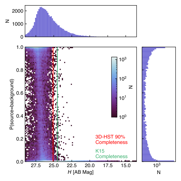
In a first test, we can locate the Momcheva et al. 2016 catalog objects based on their reported coordinates in the Morpheus background image, and then record the background pixel values at those locations. Figure 21 shows the two-dimensional histogram of Morpheus background value and 3D-HST source -band AB magnitude, along with the marginal distributions of both quantities. The figure also indicates the reported K15 sample and 3D-HST 90% completeness flux levels. The results demonstrate that for the majority of 3D-HST sources and for the vast majority of bright 3D-HST sources with , the local Morpheus background. The low background values computed by Morpheus extend to extremely faint magnitudes (e.g., ), indicating that for some faint sources, Morpheus reports background and that background is not a simple function of the local of an object. For many objects with fluxes below the 3D-HST completeness, the Morpheus background value does increase with decreasing flux, and there is a rapid transition between detected sources at to undetected sources at .
Owing to this transition in background with decreasing flux, the completeness of Morpheus relative to 3D-HST will depend on a threshold in background used to define a detection. Figure 22 shows the completeness of Morpheus in recovering 3D-HST objects as a function of -band source flux for different background levels defining a Morpheus detection. The completeness flux limits for K15 and 3D-HST are indicated for reference. For magnitudes AB, where 3D-HST and K15 are complete, Morpheus is highly complete and recovers more than of all 3D-HST sources. The Morpheus completeness declines rapidly at fluxes AB, where Morpheus is 90% relative to 3D-HST for background thresholds of . Perhaps remarkably, for all background thresholds Morpheus detects some objects as faint as , about fainter in flux than the training set objects.
We further examined the detection of 3D-HST sources as a function of color (-) to evaluate bias that may have been inherited as result of the training dataset. In our tests, we found that Morpheus is not biased with respect to color for those sources which are brighter than the K15 magnitude limit (Figure 23). When considering all sources within the 3D-HST catalog, Morpheus detects sources well, with a slight bias for bluer sources, but performs less well for very red () and () sources. However, it should be noted that there are very few such sources in the training set, and with a more extensive training sample, Morpheus could be more complete.
VII.5 Morphological Classification vs. Source Magnitude
The tests of Morpheus on simulated Sersic objects of different effective radii and the completeness study suggest that the ability of Morpheus to provide informative morphological information about astronomical sources will depend on the size and signal-to-noise of the object. While these are intuitive limitations on any morphological classification method, the distribution of morphological classifications with source flux determined by Morpheus should be quantified.
Figure 24 shows the fraction of 3D-HST objects detected and classified by Morpheus as spheroid, disk, irregular, and point source/compact as a function of their -band magnitude. Most of the brightest objects in the image are nearby stars, classified as point source/compact. At intermediate magnitudes, Morpheus classifies the objects as primarily a mix of disk () and spheroid (), with contributions from irregular () and point source/compact (). For fainter objects, below the completeness limit of the K15 training sample, Morpheus increasingly classifies objects as irregular and point source/compact. This behavior is in part physical, in that many low mass galaxies are irregular and distant galaxies are physically compact. In part, it reflects a natural bias in how the morphologies are defined during training. In K15, the class point/source compact can describe bright stars and compact unresolved sources (see Section 3.1 of K15). However, the trend also reflects how Morpheus becomes less effective at distinguishing morphologies in small, faint objects and returns either point source/compact and irregular for low and compact sources. While training Morpheus on fainter objects with well-defined morphologies could enhance the ability of Morpheus to distinguish the features of faint sources, the results of this test make sense in the context of the completeness limit of the K15 training sample used.
VII.6 False Positives in GOODS South
The segmentation and deblending of real astronomical datasets are challenging tasks. An important test of the efficacy of the Morpheus segmentation and deblending algorithms is to examine false positives generated when Morpheus is applied to a real image. To quantify the propensity for Morpheus to generate false positives, the segmentation and deblending algorithms were run on the HLF GOODS South image without the specified marker set parameter p (See Algorithms 1 and 2). For the purposes of this test, a false positive is then defined as a set of pixels classified by the Morpheus segmentation and deblending algorithms as a source but that does not contain a source from the 3DHST and CANDELS (Guo et al. 2013) catalogs. Additionally, since the edges of the GOODS South classified image are a frayed mix of pixels, to minimize the effects of data artifacts sources less than 20 pixels from the edge of the classified area were excluded from the analysis. Further, we conservatively use the “default” Morpheus algorithms that identify sources with , i.e., when Morpheus indicates a source detection with high confidence. With these choices, the sample used for the false positive analysis was a total of 19,481 sources.
Among the objects classified by the segmentation and deblending algorithms, 123 sources were not present in the CANDELS or 3D-HST catalogs. Upon visual inspection of these sources, each can be categorized as an image artifact, a poor deblend, a missed source, or an actual false positive. We list the number of sources in each category in Table 4.
Sources in the image artifiact category are false positives caused by image artifacts. The poor deblend category represents false positives caused by the Morpheus deblending algorithm, where single sources in the CANDELS or 3D-HST catalogs were shredded into multiple Morpheus sources. The missed sources are Morpheus sources that upon visual inspection correspond to real objects missed by the 3D-HST or CANDELS catalogs. Sources in the actual false positive category are false positives not associated with any image artifact or real source after visual inspection.
As Table 4 shows, Morpheus can identify real sources that other methods used to generate catalogs can miss, although the algorithms used by Morpheus can very rarely cause actual false positives (at roughly the rate). Given the delicate nature of deblending, this analysis suggests that the Morpheus deblending algorithm could be integrated with other methods to generate more robust segmentation maps.
| False Positives in GOODS South | |||
|---|---|---|---|
| Category | Count | % of False Positives | % of All Sources |
| Image Artifact | |||
| Poor Deblend | |||
| Missed Source | |||
| Actual False Positive | |||
| Total | 123 | 100% | 0.631% |
VIII Value Added Catalog for 3D-HST Sources with Morpheus Morphologies
The Morpheus framework provides a system for performing the pixel-level analysis of astronomical images and has been engineered to allow for the processing of large-format scientific FITS data. As described in Section VI.1, Morpheus was applied to the Hubble Legacy Fields (Illingworth et al. 2016, HLF;) reduction of HST imaging in GOODS South22 2 Some bright pixels in the released HLF images are censored with zeros. For the purpose of computing the segmentation maps only, we replaced these censored pixels with nearby flux values. and a suite of morphological classification images produced. Using the Morpheus background in GOODS South, the detection efficiency of Morpheus relative to the Momcheva et al. 2016 3D-HST catalog was computed (see Section VII.4) and a high level of completeness demonstrated for objects comparably bright to the Kartaltepe et al. 2015 galaxy sample used to train the model. By segmenting and deblending the HLF images, Morpheus can then compute flux-weighted morphologies for all the 3D-HST sources.
Table 5 provides the Morpheus morphological classifications for sources from the 3D-HST catalog of Momcheva et al. 2016. This value-added catalog lists the 3D-HST ID, the source right ascension and declination, the -band AB magnitude (or for negative flux objects), and properties for the sources computed by Morpheus. The value-added properties include a flag denoting whether and how Morpheus detected the object, the area in pixels assigned to each source, and the spheroid, disk, irregular, point source/compact, and background flux-weighted classifications determined by Morpheus. The size of the segmentation regions assigned to each 3D-HST object following Algorithms 1 and 2 is reported for all objects. If the segmentation region assigned to an object was smaller than a circle with a 0.36” radius, or the object was undetected, instead, use a 0.36” radius aperture (about 109 pixels) to measure flux-weighted quantities. Only objects with joint coverage in the HLF , , , and FITS images are classified and receive an assigned pixel area. The full results for the Morpheus morphological classifications of 3D-HST objects are released as a machine-readable table accompanying this paper. Appendix D describes the Morpheus Data Release associated with this paper, including FITS images of the classification images, the value-added catalog, and segmentation maps generated by Morpheus for the 3D-HST sources used to compute flux-weighted morphologies. Additionally, we release an interactive online map at https://morpheus-project.github.io/morpheus/, which provides an interface to examine the data and overlay the 3D-HST catalog on the Morpheus classification images, morphological color images, and segmentation maps.
| ID | RA | Dec | Detection | Area | spheroid | disk | irregular | ps/compact | background | min(background) | |
|---|---|---|---|---|---|---|---|---|---|---|---|
| [deg] | [deg] | [AB mag] | Flag | [pixels] | |||||||
| 1 | 53.093012 | -27.954546 | 19.54 | 1 | 4408 | 0.092 | 0.797 | 0.106 | 0.003 | 0.003 | 0.000 |
| 2 | 53.089613 | -27.959742 | 25.49 | 0 | – | – | – | – | – | – | – |
| 3 | 53.102913 | -27.959642 | 25.37 | 1 | 121 | 0.013 | 0.033 | 0.894 | 0.025 | 0.034 | 0.000 |
| 4 | 53.101709 | -27.958481 | 21.41 | 1 | 725 | 0.001 | 0.874 | 0.120 | 0.004 | 0.001 | 0.000 |
| 5 | 53.102277 | -27.958683 | 24.62 | 1 | 144 | 0.098 | 0.003 | 0.020 | 0.746 | 0.133 | 0.000 |
| 6 | 53.090577 | -27.958515 | 25.07 | 2 | 109 | 0.000 | 0.831 | 0.034 | 0.000 | 0.134 | 0.001 |
| 7 | 53.099964 | -27.958278 | 23.73 | 1 | 266 | 0.000 | 0.712 | 0.284 | 0.000 | 0.003 | 0.000 |
| 8 | 53.096144 | -27.957583 | 21.41 | 1 | 1322 | 0.001 | 0.752 | 0.238 | 0.003 | 0.006 | 0.000 |
| 9 | 53.091572 | -27.958367 | 25.90 | 2 | 109 | 0.000 | 0.044 | 0.083 | 0.081 | 0.792 | 0.431 |
| 10 | 53.091852 | -27.958181 | 25.88 | 2 | 109 | 0.000 | 0.000 | 0.038 | 0.186 | 0.776 | 0.570 |
Column 1 provides the 3D-HST source ID. Columns 2 and 3 list the right ascension and declination in degrees. Column 4 shows the AB magnitude of the 3D-HST source, with indicating a negative flux reported by 3D-HST. Column 5 lists the detection flag, with 0 indicating the object was not within the region of GOODS South classified by Morpheus, 1 indicating a detection with background at the source location, 2 indicating a possible detection with background at the source location, and 3 indicating a non-detection with background at the source location. Column 6 reports the area in pixels for the object determined by the Morpheus segmentation algorithm. For non-detections and objects with very small segmentation regions, we instead use a 0.36” radius circle (about 109 pixels) for their segmentation region. Columns 7-11 list the flux-weighted Morpheus morphological classifications of the objects within their assigned area. These columns are normalized such that the classifications sum to one for objects where the detection flag . Column 12 reports the minimum background value within the segmentation region. Table 5 is published in its entirety in the machine-readable format along with comparable tables for the other CANDELS fields. A portion is shown here for guidance regarding its form and content.
IX Discussion
The analysis of astronomical imagery necessarily involves pixel-level information to be used to characterize sources. The semantic segmentation approach of Morpheus delivers pixel-level separation between sources and the background sky, and provides an automated classification of the source pixels. In this paper, we trained Morpheus with the visual morphological classifications from Kartaltepe et al. 2015. We then characterized the performance of Morpheus in reproducing the object-level classifications of K15 after aggregating the pixel information through flux-weighted averages of pixels in Morpheus-derived segmentation maps, and in detecting objects via completeness measured relative to the 3D-HST catalog (Momcheva et al. 2016). The potential applications of Morpheus extend well beyond object-level morphological classification. Below, we discuss some applications of the pixel-level information to understanding the complexities of galaxy morphology and future applications of the semantic segmentation approach of Morpheus in areas besides morphological classification. We also comment on some features of Morpheus specific to its application on astronomical images.
IX.1 Pixel-Level Morphology
The complex morphologies of astronomical objects have been described by both visual classification schemes and quantitative morphological measures for many years. Both Hubble 1926 and Vaucouleurs 1959 sought to subdivide broad morphological classifications into more descriptive categories. Quantitative morphological decompositions of galaxies (Peng et al. 2010, e.g.,) also characterize the relative strength of bulge and disk components in galaxies, and quantitative morphological classifications often measure the degree of object asymmetry (Abraham et al. 1994; Conselice et al. 2000; Lotz et al. 2004, e.g.,).
The object-level classifications computed by Morpheus provide a mixture of the pixel-level morphologies from the Morpheus classification images. The classification distributions reported in the Morpheus value-added catalog in GOODS South provide many examples of flux-weighted measures of morphological type. However, more information is available in the pixel-level classifications than flux-weighted summaries provide.
Figure 25 shows an example object for which the Morpheus pixel-level classifications provide direct information about its complex morphology. The figure shows a disk galaxy with a prominent central bulge. The pixel-level classifications capture both the central bulge and the extended disk, with the pixels in each structural component receiving dominant bulge or disk classifications from Morpheus. Note that Morpheus was not trained to perform this automated bulge–disk decomposition, as in the training process, all pixels in a given object are assigned the same distribution of classifications as determined by the K15 visual classifiers. As the use of pixel-level morphological classifications becomes wide-spread, the development of standard datasets that include labels at the pixel-level will be needed to evaluate the efficacy of classifiers. Simulations of galaxy formation may be useful for generating such training datasets (Huertas-Company et al. 2019, e.g.,). We leave a more thorough analysis of automated morphological decompositions with Morpheus to future work.


IX.2 Morphological Deblending
The ability of Morpheus to provide pixel-level morphological classifications has applications beyond the bulk categorization of objects. One potential additional application is the morphological deblending of overlapping objects, where the pixel-level classifications are used to augment the deblending process. Figure 26 shows an example of two blended objects, 3D-HST IDs 543 and 601, where the Morpheus pixel-level classifications could be used to perform or augment star-galaxy separation. As the figure makes clear, when Morpheus correctly assigns dominant classifications to pixels, there exists an interface region between regions with distinctive morphologies (in this case, spheroid and point source/compact) that could serve as an interface between segmented regions in the image. The deblending algorithm used in this work could include other forms of machine learning (Masters et al. 2015; Hemmati et al. 2019, e.g.,) information in the deblending process. If Morpheus was trained on information other than morphology, such as photometric redshift, those pixel-level classifications could be used in the deblending process as well. We plan to explore this idea in future applications of Morpheus.
IX.3 Classifications Beyond Morphology
The semantic segmentation approach of Morpheus allows for complex features of astronomical objects to be learned from the data, as long as those features can be spatially localized by other means. In this paper, we used the segmentation maps of K15 to separate source pixels from the sky, and then assigned pixels within the segmentation maps the morphological classification determined by K15 on an object-by-object basis. In principle, this approach can be extended to identify regions of pixels that contain a wide variety of features. For instance, Morpheus could be trained to identify image artifacts, spurious cosmic rays, or other instrumental or data effects that lead to distinctive pixel-level features in images. Of course, real features in images could also be identified, such as the pixels containing arcs in gravitational lenses, or perhaps low-surface brightness features in interacting systems and stellar halos. These pixel-level applications of Morpheus complement machine learning-based methods already deployed, such as those that discover and model gravitational lenses (Agnello et al. 2015; Hezaveh et al. 2017; Morningstar et al. 2018; Morningstar et al. 2019). Pixel-level photometric redshift estimates could also be adopted by Morpheus and compared with existing methods based on SED fitting or other forms of machine learning (Masters et al. 2015; Hemmati et al. 2019, e.g.,).
IX.4 Deep Learning and Astronomical Imagery
An important difference in the approach of Morpheus, where a purpose-built framework was constructed from TensorFlow primitives, compared with the adaptation and retraining of existing frameworks like Inception (Szegedy et al. 2016, e.g.,) is the use of astronomical FITS images as training, test, and input data rather than preprocessed PNG or JPG files. The incorporation of deep learning into astronomical pipelines will benefit from the consistency of the data format. The output data of Morpheus are also FITS classification images, allowing pixel-by-pixel information to be easily referenced between the astronomical science images and the Morpheus model images. As indicated in Section II.2, the Morpheus framework is extensible and allows for any number of astronomical filter images to be used, as opposed to a fixed red-blue-green set of layers in PNG or JPG files. The Morpheus framework has been engineered to allow for the classification of arbitrarily-sized astronomical images. The same approach also provides Morpheus a measure of the dispersion of the classifications of individual pixels, allowing the user to choose a metric for the “best” pixel-by-pixel classification. The combination of these features allows for immense flexibility in adapting the Morpheus framework to problems in astronomical image classification.
X Summary and Conclusions
In this paper, we presented Morpheus, a deep learning framework for the pixel-level analysis of astronomical images. The architecture of Morpheus consists of our original implementation of a U-Net (Ronneberger et al. 2015) convolutional neural network. Morpheus applies the semantic segmentation technique adopted from computer vision to enable pixel-by-pixel classifications, and by separately identifying background and source pixels Morpheus combines object detection and classification into a single analysis. Morpheus represents a new approach to astronomical data analysis, with wide applicability in enabling per-pixel classification of images where suitable training datasets exist. Important results from this paper include:
- •
Morpheus provides pixel-level classifications of astronomical FITS images. By using user-supplied segmentation maps during training, the model learns to distinguish background pixels from pixels containing source flux. The pixels associated with astronomical objects are then classified according to the classification scheme of the training data set. The entire Morpheus source code has been publicly released, and a Python package installer for Morpheus provided. Further, we have a citable “frozen” version of code available through Zenodo (Hausen 2020).
- •
As a salient application, we trained Morpheus to provide pixel-level classifications of galaxy morphology by using the Kartaltepe et al. 2015 visual morphological classifications of galaxies in the CANDELS dataset (Grogin et al. 2011; Koekemoer et al. 2011) as our training sample.
- •
Applying Morpheus to the Hubble Legacy Fields (Illingworth et al. 2016) v2.0 reduction of the CANDELS data in GOODS South and the v1.0 data (Grogin et al. 2011; Koekemoer et al. 2011) for COSMOS, EGS, GOODS North and UDS, we generated morphological classifications for every pixel in the HLF mosaics. The resulting Morpheus morphological classification images have been publicly released.
- •
The pixel-level morphological classifications in GOODS South were then used to compute and publicly release a “value-added” catalog of morphologies for all objects in the public 3D-HST source catalog (Skelton et al. 2014; Momcheva et al. 2016).
- •
The CANDELS HLF and 3D-HST data were used to quantify the performance of Morpheus, both for morphological classification and its completeness in object detection. As trained, the Morpheus code shows high completeness at magnitudes AB. We demonstrate that Morpheus can detect objects in astronomical images at flux levels up to fainter than the completeness limit of its training sample (AB).
- •
Tutorials for using the Morpheus deep learning framework have been created and publicly released as Jupyter notebooks.
- •
An interactive visualization of the Morpheus model results for GOODS South, including the Morpheus segmentation maps and pixel-level morphological classifications of 3D-HST sources, has been publicly released.
We expect that semantic segmentation will be increasingly used in astronomical applications of deep learning, and Morpheus serves as an example framework that leverages this technique to identify and classify objects in astronomical images. We caution that Morpheus may be most effective at wavelengths similar to the data on which the model was trained (i.e., the , , , and bands). However, Domínguez Sánchez et al. 2019 have shown recent success in applying transfer learning on astronomical datasets with morphological labels. With the advent of large imaging data sets such those provided by Dark Energy Survey (Dark Energy Survey Collaboration et al. 2016) and Hyper Suprime-Cam (Aihara et al. 2018a; Aihara et al. 2018b), and next-generation surveys to be conducted by Large Synoptic Survey Telescope (Ivezić et al. 2019; Robertson et al. 2019), Euclid (Laureijs et al. 2011; Rhodes et al. 2017), and the Wide Field Infrared Survey Telescope (Akeson et al. 2019), pixel-level analysis of massive imaging data sets with deep learning will find many applications. While the details of the Morpheus neural network architecture will likely change and possibly improve, we expect the approach of using semantic segmentation to provide pixel-level analyses of astronomical images with deep learning models will be broadly useful. The public release of the Morpheus code, tutorials, and example data products should provide a basis for future applications of deep learning for astronomical datasets.
Appendix A Deep Learning
The Morpheus deep learning framework incorporates a variety of technologies developed for machine learning applications. The following descriptions of deep learning techniques complement the overview of Morpheus provided in Section II, and are useful for understanding optional configurations of the model.
A.1 Artificial Neuron
The basic unit of the Morpheus neural network is the artificial neuron (AN), which transforms an input vector to a single output . The AN is designed to mimic the activation of a neuron, producing a nonlinear response to an input stimulus value when it exceeds a rough threshold.
The first stage of an AN consists of a function
| (A1) |
that adds the dot product of the -element vector with a vector of weights to a bias . The values of the elements and are parameters of the model that are set during optimization. The function is equivalent to a linear transformation on input data .
In the second stage, a nonlinear function is applied to the output of . We write
| (A2) |
where is called the activation function. The Morpheus framework allows the user to specify the activation function, including the sigmoid
| (A3) |
the hyperbolic tangent
| (A4) |
and the rectified linear unit
| (A5) |
These functions share a thresholding behavior, such that the function activates a nonlinear behavior at a characteristic value of , but the domain of these functions differ. For the morphological classification problem presented in this paper, the rectified linear unit (Equation A5) was used as the activation function.
A.2 Neural Networks
Increasingly complex computational structures can be constructed from ANs. Single ANs are combined into layers, which are collections of distinct ANs that process the same input vector . A collection of layers forms a neural network (NN), with the layers ordered such that the outputs from one layer provide the inputs to the neurons in the subsequent layer. Figure 27 shows a schematic of a NN and how the initial input vector is processed by multiple layers. As shown, these layers are commonly called fully-connected since each neuron in a given layer receives the outputs from all neurons in the previous layer.
A.3 Convolutional Neural Networks
The Morpheus framework operates on image data with a convolutional neural network (CNN). A CNN includes at least one layer of ANs whose z function uses a discrete cross-correlation (convolution) in place of the dot product in Equation A1. For a convolutional artificial neuron (CAN), we write
| (A6) |
where represents the convolution of an input image and a kernel . The elements of the kernel are parameters of the model, and may differ in dimensions from . In Morpheus, the dimensions of are set to be throughout. The bias is a scalar as before, and represents a matrix of s with the same dimensions as the result of the convolution. In Morpheus, the convolution is zero-padded to maintain the dimensions of the input data.
The activation function of the neuron is computed element-wise after the convolution and bias have been applied to the input. We write
| (A7) |
We refer to the output from a CAN as a feature map.
As with fully-connected layers, convolutional layers consist of a group of CANs that process the same input data . Convolutional layers can also be arranged sequentially such that the output from one convolutional layer serves as input to the next. Morpheus’ neural network architecture, being U-Net based, is comprised of CANs (see Figure 28 for a schematic). In typical convolutional neural network topologies, CANs are used to extract features from input images. The resulting feature maps are eventually flattened into a single vector and processed by a fully connected layer to produce the output classification values.

A.4 Other Functions in Neural Networks
The primary computational elements of Morpheus are a convolutional neural network (Section A.3) and a fully connected layer (Section A.2). In detail, other layers are used to reformat or summarize the data, renormalize it, or combine data from different stages in the network.
A.4.1 Pooling
Pooling layers (Figure 29) are composed of functions that summarize their input data to reduce its size while preserving some information. These layers perform a moving average (average pooling) or maximum (max pooling) over a window of data elements, repeating these reductions as the window scans through the input image with a stride equal to the window size. In the morphological classification tasks described in this paper, Morpheus uses windows and max pooling.
A.4.2 Up-sampling
Up-sampling layers expand the size of feature maps by a specified factor through an interpolation between input data elements. The up-sampling layers operate in the image dimensions of the feature map and typically employ bicubic and bilinear interpolation. In the morphological classification application explored in this paper, Morpheus used up-sampling and bicubic interpolation.
A.4.3 Concatenation
Concatenation layers combine multiple feature maps by appending them without changing their contents. For instance, the concatenation of red, green, and blue (RGB) channels into a three-color image would append three images into an RGB image with dimensions . This operation is used in Morpheus to combine together data from the contraction phase with the output from bicubic interpolations in the expansion phase (see Figure 2).
A.4.4 Batch Normalization
A common preprocessing step for neural network architectures is to normalize the input data using, e.g., the operation
| (A8) |
where is the normalized data, and and are parameters of the model. Ioffe & Szegedy 2015 extended this normalization step to apply to the inputs of layers within the network, such that activations (AN) and feature maps (CAN) are normalized over each batch. A batch consists of a subset of the training examples used during the training process. Simple normalization operations like Equation A8 can reduce the range of values represented in the data provided to a layer, which can inhibit learning. Ioffe & Szegedy 2015 addressed this issue by providing an alternative normalization operation that introduces additional parameters to be learned during training. The input data elements are first rescaled as
| (A9) |
Here, is a single element from the data output by a single AN or CAN over a batch, is their mean, and is their variance. The parameter is learned during optimization. The new normalization is then taken to be a linear transformation
| (A10) |
The parameters and are also learned during optimization. Ioffe & Szegedy 2015 demonstrated that batch normalization, in the form of Equation A10, can increase overall accuracy and decrease training time, and we adopt this approach in the Morpheus framework.
A.5 U-Net Architecture
The Morpheus framework uses a U-Net architecture, first introduced by Ronneberger et al. 2015. The U-Net architecture was originally designed for segmentation of medical imagery, but has enjoyed success in other fields. The U-Net takes as input a set of images and outputs a classification image of pixel-level probability distributions. The architecture begins with a contraction phase composed of a series of convolutional and pooling layers, followed by an expansion phase composed of a series of convolutional and up-sampling layers. Each of the outputs from the down-sampling layers is concatenated with the output of an up-sampling layer when the height and width dimensions of the feature maps match. These concatenations help preserve the locality of learned features in the output of the NN.
Appendix B code release
The code for Morpheus has been release via GitHub (https://github.com/morpheus-project/morpheus). Morpheus is also available as a python package installable via pip (https://pypi.org/project/morpheus-astro/) and as Docker images available via Docker Hub (https://hub.docker.com/r/morpheusastro/morpheus). Morpheus includes both a Python API and a command-line interface, the documentation of which can be found online at https://morpheus-astro.readthedocs.io/en/latest/.
Appendix C code tutorial
An online tutorial demonstrating the Morpheus Python API in the form of a Jupyter
notebook can be found at
https://github.com/morpheus-project/morpheus/blob/master/examples/example_array.ipynb.
The tutorial walks through the classification of an example image. Additionally,
the tutorial explores other features of Morpheus, including generating
segmentation maps and morphological catalogs.
Appendix D Data Release
The data release associated with this work consists of multiple data products. For each field in the CANDELS survey, we provide the following data products: pixel-level morphological classifications, segmentation maps, and value-added catalogs(see also Section VIII) for the 3D-HST catalogs. Tables 6-10 provide the URLs for each of the data products. Each of the fields has two types of segmentation maps, a segmentation map informed by the 3D-HST survey and a segmentation map informed only by the background values provided by Morpheus (see Algorithm 1). The classifications for the EGS and UDS fields may vary as a result of using the band in place of the due to availability.
An interactive online visualization of the HST images, Morpheus classification images, and 3D-HST sources is available at https://morpheus-project.github.io/morpheus/.


Morpheus Data Products for the COSMOS Field File Name URL Pixel-level Morphological Classifications morpheus_COSMOS_spheroid.v1.0.fits morpheus-project.github.io/morpheus/data-release/cosmos/spheroid.html morpheus_COSMOS_disk.v1.0.fits morpheus-project.github.io/morpheus/data-release/cosmos/disk.html morpheus_COSMOS_irregular.v1.0.fits morpheus-project.github.io/morpheus/data-release/cosmos/irregular.html morpheus_COSMOS_ps_compact.v1.0.fits morpheus-project.github.io/morpheus/data-release/cosmos/ps_compact.html morpheus_COSMOS_background.v1.0.fits morpheus-project.github.io/morpheus/data-release/cosmos/background.html morpheus_COSMOS_mask.v1.0.fits morpheus-project.github.io/morpheus/data-release/cosmos/mask.html Segmentation Maps morpheus_COSMOS_segmap.v1.0.fits morpheus-project.github.io/morpheus/data-release/cosmos/segmap.html morpheus_COSMOS_3dhst-segmap.v1.0.fits morpheus-project.github.io/morpheus/data-release/cosmos/3dhst-segmap.html 3D-HST Value Added Catalog morpheus_COSOMS_3dhst_catalog.v1.0.csv morpheus-project.github.io/morpheus/data-release/cosmos/value-added-catalog.html morpheus_COSOMS_3dhst_catalog.v1.0.txt morpheus-project.github.io/morpheus/data-release/cosmos/value-added-catalog-mrt.html All Files morpheus_COSMOS_all.v1.0.tar.gz morpheus-project.github.io/morpheus/data-release/cosmos/all.html
Morpheus Data Products for the EGS Field File Name URL Pixel-level Morphological Classifications morpheus_EGS_spheroid.v1.0.fits morpheus-project.github.io/morpheus/data-release/egs/spheroid.html morpheus_EGS_disk.v1.0.fits morpheus-project.github.io/morpheus/data-release/egs/disk.html morpheus_EGS_irregular.v1.0.fits morpheus-project.github.io/morpheus/data-release/egs/irregular.html morpheus_EGS_ps_compact.v1.0.fits morpheus-project.github.io/morpheus/data-release/egs/ps_compact.html morpheus_EGS_background.v1.0.fits morpheus-project.github.io/morpheus/data-release/egs/background.html morpheus_EGS_mask.v1.0.fits morpheus-project.github.io/morpheus/data-release/egs/mask.html Segmentation Maps morpheus_EGS_segmap.v1.0.fits morpheus-project.github.io/morpheus/data-release/egs/segmap.html morpheus_EGS_3dhst-segmap.v1.0.fits morpheus-project.github.io/morpheus/data-release/egs/3dhst-segmap.html 3D-HST Value Added Catalogs morpheus_EGS_3dhst_catalog.v1.0.csv morpheus-project.github.io/morpheus/data-release/egs/value-added-catalog.html morpheus_EGS_3dhst_catalog.v1.0.txt morpheus-project.github.io/morpheus/data-release/egs/value-added-catalog-mrt.html All Files morpheus_EGS_all.v1.0.tar.gz morpheus-project.github.io/morpheus/data-release/egs/all.html
Morpheus Data Products for the GOODS North Field File Name URL Pixel-level Morphological Classifications morpheus_GOODS-N_spheroid.v1.0.fits morpheus-project.github.io/morpheus/data-release/goods-n/spheroid.html morpheus_GOODS-N_disk.v1.0.fits morpheus-project.github.io/morpheus/data-release/goods-n/disk.html morpheus_GOODS-N_irregular.v1.0.fits morpheus-project.github.io/morpheus/data-release/goods-n/irregular.html morpheus_GOODS-N_ps_compact.v1.0.fits morpheus-project.github.io/morpheus/data-release/goods-n/ps_compact.html morpheus_GOODS-N_background.v1.0.fits morpheus-project.github.io/morpheus/data-release/goods-n/background.html morpheus_GOODS-N_mask.v1.0.fits morpheus-project.github.io/morpheus/data-release/goods-n/mask.html Segmentation Maps morpheus_GOODS-N_segmap.v1.0.fits morpheus-project.github.io/morpheus/data-release/goods-n/segmap.html morpheus_GOODS-N_3dhst-segmap.v1.0.fits morpheus-project.github.io/morpheus/data-release/goods-n/3dhst-segmap.html 3D-HST Value Added Catalogs morpheus_GOODS-N_3dhst_catalog.v1.0.csv morpheus-project.github.io/morpheus/data-release/goods-n/value-added-catalog.html morpheus_GOODS-N_3dhst_catalog.v1.0.txt morpheus-project.github.io/morpheus/data-release/goods-n/value-added-catalog-mrt.html All Files morpheus_GOODS-N_all.v1.0.tar.gz morpheus-project.github.io/morpheus/data-release/goods-n/all.html
Morpheus Data Products for the GOODS South Field File Name URL Pixel-level Morphological Classifications morpheus_GOODS-S_spheroid.v1.0.fits morpheus-project.github.io/morpheus/data-release/goods-s/spheroid.html morpheus_GOODS-S_disk.v1.0.fits morpheus-project.github.io/morpheus/data-release/goods-s/disk.html morpheus_GOODS-S_irregular.v1.0.fits morpheus-project.github.io/morpheus/data-release/goods-s/irregular.html morpheus_GOODS-S_ps_compact.v1.0.fits morpheus-project.github.io/morpheus/data-release/goods-s/ps_compact.html morpheus_GOODS-S_background.v1.0.fits morpheus-project.github.io/morpheus/data-release/goods-s/background.html morpheus_GOODS-S_mask.v1.0.fits morpheus-project.github.io/morpheus/data-release/goods-s/mask.html morpheus_GOODS-S_spheroid.v1.0.fits morpheus-project.github.io/morpheus/data-release/goods-s/spheroid.html Segmentation Maps morpheus_GOODS-S_segmap.v1.0.fits morpheus-project.github.io/morpheus/data-release/goods-s/segmap.html morpheus_GOODS-S_3dhst_segmap.v1.0.fits morpheus-project.github.io/morpheus/data-release/goods-s/3dhst-segmap.html 3D-HST Value Added Catalogs morpheus_GOODS-S_3dhst_catalog.v1.0.csv morpheus-project.github.io/morpheus/data-release/goods-s/value-added-catalog.html morpheus_GOODS-S_3dhst_catalog.v1.0.txt morpheus-project.github.io/morpheus/data-release/goods-s/value-added-catalog-mrt.html All Files morpheus_GOODS-S_all.v1.0.tar.gz morpheus-project.github.io/morpheus/data-release/goods-s/all.html
Morpheus Data Products for the UDS Field File Name URL Pixel-level Morphological Classifications morpheus_UDS_spheroid.v1.0.fits morpheus-project.github.io/morpheus/data-release/uds/spheroid.html morpheus_UDS_disk.v1.0.fits morpheus-project.github.io/morpheus/data-release/uds/disk.html morpheus_UDS_irregular.v1.0.fits morpheus-project.github.io/morpheus/data-release/uds/irregular.html morpheus_UDS_ps_compact.v1.0.fits morpheus-project.github.io/morpheus/data-release/uds/ps_compact.html morpheus_UDS_background.v1.0.fits morpheus-project.github.io/morpheus/data-release/uds/background.html morpheus_UDS_mask.v1.0.fits morpheus-project.github.io/morpheus/data-release/uds/mask.html Segmentation Maps morpheus_UDS_segmap.v1.0.fits morpheus-project.github.io/morpheus/data-release/uds/segmap.html morpheus_UDS_3dhst-segmap.v1.0.fits morpheus-project.github.io/morpheus/data-release/uds/3dhst-segmap.html 3D-HST Value Added Catalogs morpheus_UDS_3dhst_catalog.v1.0.csv morpheus-project.github.io/morpheus/data-release/uds/value-added-catalog.html morpheus_UDS_3dhst_catalog.v1.0.txt morpheus-project.github.io/morpheus/data-release/uds/value-added-catalog-mrt.html All Files morpheus_UDS_all.v1.0.tar.gz morpheus-project.github.io/morpheus/data-release/uds/all.html
References
- Abadi et al. (2016) Abadi, M., Agarwal, A., Barham, P., et al. 2016, arXiv e-prints, arXiv:1603.04467
- Abraham et al. (1996) Abraham, R. G., Tanvir, N. R., Santiago, B. X., et al. 1996, MNRAS, 279, L47
- Abraham et al. (1994) Abraham, R. G., Valdes, F., Yee, H. K. C., & van den Bergh, S. 1994, ApJ, 432, 75
- Abraham & van den Bergh (2001) Abraham, R. G., & van den Bergh, S. 2001, Science, 293, 1273. http://science.sciencemag.org/content/293/5533/1273
- Agnello et al. (2015) Agnello, A., Kelly, B. C., Treu, T., & Marshall, P. J. 2015, MNRAS, 448, 1446
- Aihara et al. (2018a) Aihara, H., Arimoto, N., Armstrong, R., et al. 2018a, PASJ, 70, S4
- Aihara et al. (2018b) Aihara, H., Armstrong, R., Bickerton, S., et al. 2018b, PASJ, 70, S8
- Akeson et al. (2019) Akeson, R., Armus, L., Bachelet, E., et al. 2019, arXiv e-prints, arXiv:1902.05569
- Allen et al. (2017) Allen, R. J., Kacprzak, G. G., Glazebrook, K., et al. 2017, ApJ, 834, L11
- Beck et al. (2018) Beck, M. R., Scarlata, C., Fortson, L. F., et al. 2018, MNRAS, 476, 5516
- Bell et al. (2012) Bell, E. F., van der Wel, A., Papovich, C., et al. 2012, ApJ, 753, 167
- Bender et al. (1992) Bender, R., Burstein, D., & Faber, S. M. 1992, ApJ, 399, 462
- Bertin & Arnouts (1996) Bertin, E., & Arnouts, S. 1996, A&AS, 117, 393
- Bezanson et al. (2013) Bezanson, R., van Dokkum, P. G., van de Sande, J., et al. 2013, ApJ, 779, L21
- Binney (1978) Binney, J. 1978, MNRAS, 183, 501
- Binney & Tremaine (1987) Binney, J., & Tremaine, S. 1987, Galactic dynamics (Princeton, NJ: Princeton University Press)
- Boucaud et al. (2019) Boucaud, A., Huertas-Company, M., Heneka, C., et al. 2019, arXiv e-prints, arXiv:1905.01324
- Bruce et al. (2016) Bruce, V. A., Dunlop, J. S., Mortlock, A., et al. 2016, MNRAS, 458, 2391
- Bruce et al. (2012) Bruce, V. A., Dunlop, J. S., Cirasuolo, M., et al. 2012, MNRAS, 427, 1666
- Cireşan et al. (2012) Cireşan, D., Meier, U., & Schmidhuber, J. 2012, arXiv e-prints, arXiv:1202.2745
- Conselice (2003) Conselice, C. J. 2003, ApJS, 147, 1
- Conselice et al. (2000) Conselice, C. J., Bershady, M. A., & Jangren, A. 2000, ApJ, 529, 886
- Conselice et al. (2005) Conselice, C. J., Blackburne, J. A., & Papovich, C. 2005, ApJ, 620, 564
- Cooper et al. (2012) Cooper, M. C., Griffith, R. L., Newman, J. A., et al. 2012, MNRAS, 419, 3018
- Couprie & Bertrand (1997) Couprie, M., & Bertrand, G. 1997, in Society of Photo-Optical Instrumentation Engineers (SPIE) Conference Series, Vol. 3168, Vision Geometry VI, ed. R. A. Melter, A. Y. Wu, & L. J. Latecki, 136–146
- Dai & Tong (2018) Dai, J.-M., & Tong, J. 2018, ArXiv e-prints, arXiv:1807.10406
- Dark Energy Survey Collaboration et al. (2016) Dark Energy Survey Collaboration, Abbott, T., Abdalla, F. B., et al. 2016, MNRAS, 460, 1270
- Deng et al. (2009) Deng, J., Dong, W., Socher, R., et al. 2009, in CVPR09
- Dieleman et al. (2015) Dieleman, S., Willett, K. W., & Dambre, J. 2015, MNRAS, 450, 1441
- Dimauro et al. (2018) Dimauro, P., Huertas-Company, M., Daddi, E., et al. 2018, MNRAS, 478, 5410
- Djorgovski & Davis (1987) Djorgovski, S., & Davis, M. 1987, ApJ, 313, 59
- Domínguez Sánchez et al. (2019) Domínguez Sánchez, H., Huertas-Company, M., Bernardi, M., et al. 2019, MNRAS, 484, 93
- Dressler (1980) Dressler, A. 1980, ApJ, 236, 351
- Dressler et al. (1987) Dressler, A., Lynden-Bell, D., Burstein, D., et al. 1987, ApJ, 313, 42
- Dressler et al. (1997) Dressler, A., Oemler, Jr., A., Couch, W. J., et al. 1997, ApJ, 490, 577
- Elmegreen et al. (2005) Elmegreen, D. M., Elmegreen, B. G., Rubin, D. S., & Schaffer, M. A. 2005, ApJ, 631, 85
- Franx et al. (2008) Franx, M., van Dokkum, P. G., Förster Schreiber, N. M., et al. 2008, ApJ, 688, 770
- Gardner et al. (2006) Gardner, J. P., Mather, J. C., Clampin, M., et al. 2006, Space Sci. Rev., 123, 485
- González et al. (2018) González, R. E., Muñoz, R. P., & Hernández, C. A. 2018, ArXiv e-prints, arXiv:1809.01691
- Grogin et al. (2011) Grogin, N. A., Kocevski, D. D., Faber, S. M., et al. 2011, ApJS, 197, 35
- Guo et al. (2013) Guo, Y., Ferguson, H. C., Giavalisco, M., et al. 2013, ApJS, 207, 24
- Hahnloser et al. (2000) Hahnloser, R. H. R., Sarpeshkar, R., Mahowald, M. A., Douglas, R. J., & Seung, H. S. 2000, Nature, 405, 947
- Hausen (2020) Hausen, R. 2020, morpheus-project/morpheus: Zenodo Release, vv0.4.6, Zenodo, doi:10.5281/zenodo.3601680. https://doi.org/10.5281/zenodo.3601680
- Hemmati et al. (2019) Hemmati, S., Capak, P., Masters, D., et al. 2019, ApJ, 877, 117
- Hezaveh et al. (2017) Hezaveh, Y. D., Perreault Levasseur, L., & Marshall, P. J. 2017, Nature, 548, 555
- Hocking et al. (2018) Hocking, A., Geach, J. E., Sun, Y., & Davey, N. 2018, MNRAS, 473, 1108
- Hubble (1926) Hubble, E. P. 1926, ApJ, 64, doi:10.1086/143018
- Huertas-Company et al. (2015) Huertas-Company, M., Gravet, R., Cabrera-Vives, G., et al. 2015, The Astrophysical Journal Supplement Series, 221, 8
- Huertas-Company et al. (2016) Huertas-Company, M., Bernardi, M., Pérez-González, P. G., et al. 2016, MNRAS, 462, 4495
- Huertas-Company et al. (2018) Huertas-Company, M., Primack, J. R., Dekel, A., et al. 2018, ApJ, 858, 114
- Huertas-Company et al. (2019) Huertas-Company, M., Rodriguez-Gomez, V., Nelson, D., et al. 2019, MNRAS, 489, 1859
- Hunter (2007) Hunter, J. D. 2007, Computing in Science Engineering, 9, 90
- Illingworth et al. (2016) Illingworth, G., Magee, D., Bouwens, R., et al. 2016, arXiv e-prints, arXiv:1606.00841
- Ioffe & Szegedy (2015) Ioffe, S., & Szegedy, C. 2015, ArXiv e-prints, arXiv:1502.03167
- Ivezić et al. (2019) Ivezić, Ž., Kahn, S. M., Tyson, J. A., et al. 2019, ApJ, 873, 111
- Jiang et al. (2018) Jiang, D., Liu, F. S., Zheng, X., et al. 2018, ApJ, 854, 70
- Kartaltepe et al. (2015) Kartaltepe, J. S., Mozena, M., Kocevski, D., et al. 2015, ApJS, 221, 11
- Kawinwanichakij et al. (2017) Kawinwanichakij, L., Papovich, C., Quadri, R. F., et al. 2017, ApJ, 847, 134
- Kelly & McKay (2004) Kelly, B. C., & McKay, T. A. 2004, AJ, 127, 625
- Kelly & McKay (2005) Kelly, B. C., & McKay, T. A. 2005, The Astronomical Journal, 129, 1287. http://stacks.iop.org/1538-3881/129/i=3/a=1287
- Kingma & Ba (2014) Kingma, D. P., & Ba, J. 2014, ArXiv e-prints, arXiv:1412.6980
- Kocevski et al. (2012) Kocevski, D. D., Faber, S. M., Mozena, M., et al. 2012, ApJ, 744, 148
- Koekemoer et al. (2011) Koekemoer, A. M., Faber, S. M., Ferguson, H. C., et al. 2011, ApJS, 197, 36
- Kormendy (1977) Kormendy, J. 1977, ApJ, 218, 333
- Krist et al. (2011) Krist, J. E., Hook, R. N., & Stoehr, F. 2011, in Society of Photo-Optical Instrumentation Engineers (SPIE) Conference Series, Vol. 8127, Optical Modeling and Performance Predictions V, 81270J
- Laureijs et al. (2011) Laureijs, R., Amiaux, J., Arduini, S., et al. 2011, arXiv e-prints, arXiv:1110.3193
- Lecun et al. (2015) Lecun, Y., Bengio, Y., & Hinton, G. 2015, Nature, 521, 436
- Lee et al. (2013) Lee, B., Giavalisco, M., Williams, C. C., et al. 2013, ApJ, 774, 47
- Lintott et al. (2008) Lintott, C. J., Schawinski, K., Slosar, A., et al. 2008, MNRAS, 389, 1179
- Lofthouse et al. (2017) Lofthouse, E. K., Kaviraj, S., Conselice, C. J., Mortlock, A., & Hartley, W. 2017, MNRAS, 465, 2895
- Lotz et al. (2004) Lotz, J. M., Primack, J., & Madau, P. 2004, AJ, 128, 163
- Lotz et al. (2008) Lotz, J. M., Davis, M., Faber, S. M., et al. 2008, ApJ, 672, 177
- LSST Science Collaboration et al. (2009) LSST Science Collaboration, Abell, P. A., Allison, J., et al. 2009, arXiv e-prints, arXiv:0912.0201
- Margalef-Bentabol et al. (2016) Margalef-Bentabol, B., Conselice, C. J., Mortlock, A., et al. 2016, MNRAS, 461, 2728
- Masters et al. (2015) Masters, D., Capak, P., Stern, D., et al. 2015, ApJ, 813, 53
- Merkel (2014) Merkel, D. 2014, Linux J., 2014
- Miller et al. (2019) Miller, T. B., van Dokkum, P., Mowla, L., & van der Wel, A. 2019, ApJ, 872, L14
- Milletari et al. (2016) Milletari, F., Navab, N., & Ahmadi, S.-A. 2016, ArXiv e-prints, arXiv:1606.04797
- Momcheva et al. (2016) Momcheva, I. G., Brammer, G. B., van Dokkum, P. G., et al. 2016, ApJS, 225, 27
- Morishita et al. (2014) Morishita, T., Ichikawa, T., & Kajisawa, M. 2014, ApJ, 785, 18
- Morningstar et al. (2018) Morningstar, W. R., Hezaveh, Y. D., Perreault Levasseur, L., et al. 2018, arXiv e-prints, arXiv:1808.00011
- Morningstar et al. (2019) Morningstar, W. R., Perreault Levasseur, L., Hezaveh, Y. D., et al. 2019, arXiv e-prints, arXiv:1901.01359
- Novikov et al. (2017) Novikov, A. A., Lenis, D., Major, D., et al. 2017, ArXiv e-prints, arXiv:1701.08816
- Oke & Gunn (1983) Oke, J. B., & Gunn, J. E. 1983, ApJ, 266, 713
- Patel et al. (2013) Patel, S. G., Fumagalli, M., Franx, M., et al. 2013, ApJ, 778, 115
- Pedregosa et al. (2011) Pedregosa, F., Varoquaux, G., Gramfort, A., et al. 2011, Journal of Machine Learning Research, 12, 2825
- Peng et al. (2010) Peng, C. Y., Ho, L. C., Impey, C. D., & Rix, H.-W. 2010, AJ, 139, 2097
- Peth et al. (2016) Peth, M. A., Lotz, J. M., Freeman, P. E., et al. 2016, MNRAS, 458, 963
- Powell et al. (2017) Powell, M. C., Urry, C. M., Cardamone, C. N., et al. 2017, ApJ, 835, 22
- Pratt (1993) Pratt, L. Y. 1993, in Advances in Neural Information Processing Systems 5, ed. S. J. Hanson, J. D. Cowan, & C. L. Giles (Morgan-Kaufmann), 204–211. http://papers.nips.cc/paper/641-discriminability-based-transfer-between-neural-networks.pdf
- Price-Whelan et al. (2018) Price-Whelan, A. M., Sipőcz, B. M., Günther, H. M., et al. 2018, AJ, 156, 123
- Rhodes et al. (2017) Rhodes, J., Nichol, R. C., Aubourg, É., et al. 2017, ApJS, 233, 21
- Roberts & Haynes (1994) Roberts, M. S., & Haynes, M. P. 1994, ARA&A, 32, 115
- Robertson et al. (2017) Robertson, B. E., Banerji, M., Cooper, M. C., et al. 2017, arXiv e-prints, arXiv:1708.01617
- Robertson et al. (2019) Robertson, B. E., Banerji, M., Brough, S., et al. 2019, Nature Reviews Physics, doi:10.1038/s42254-019-0067-x. https://doi.org/10.1038/s42254-019-0067-x
- Ronneberger et al. (2015) Ronneberger, O., Fischer, P., & Brox, T. 2015, ArXiv e-prints, arXiv:1505.04597
- Rossum (1995) Rossum, G. 1995, Python Reference Manual, Tech. rep., Amsterdam, The Netherlands, The Netherlands
- Rumelhart et al. (1986) Rumelhart, D. E., Hinton, G. E., & Williams, R. J. 1986, Nature, 323, 533
- Russakovsky et al. (2015) Russakovsky, O., Deng, J., Su, H., et al. 2015, International Journal of Computer Vision (IJCV), 115, 211
- Sersic (1968) Sersic, J. L. 1968, Atlas de Galaxias Australes (Cordoba, Argentina: Observatorio Astronomico)
- Shen et al. (2003) Shen, S., Mo, H. J., White, S. D. M., et al. 2003, MNRAS, 343, 978
- Sheth et al. (2008) Sheth, K., Elmegreen, D. M., Elmegreen, B. G., et al. 2008, ApJ, 675, 1141
- Sheth et al. (2010) Sheth, K., Regan, M., Hinz, J. L., et al. 2010, PASP, 122, 1397
- Shibuya et al. (2015) Shibuya, T., Ouchi, M., & Harikane, Y. 2015, ApJS, 219, 15
- Simmons et al. (2014) Simmons, B. D., Melvin, T., Lintott, C., et al. 2014, MNRAS, 445, 3466
- Simmons et al. (2017) Simmons, B. D., Lintott, C., Willett, K. W., et al. 2017, MNRAS, 464, 4420
- Skelton et al. (2014) Skelton, R. E., Whitaker, K. E., Momcheva, I. G., et al. 2014, ApJS, 214, 24
- Smail et al. (1997) Smail, I., Dressler, A., Couch, W. J., et al. 1997, ApJS, 110, 213
- Smith & Geach (2019) Smith, M. J., & Geach, J. E. 2019, arXiv e-prints, arXiv:1904.10286
- Sobel & Feldman (1968) Sobel, I., & Feldman, G. 1968, presented at the Stanford Artificial Intelligence Project
- Sudre et al. (2017) Sudre, C. H., Li, W., Vercauteren, T., Ourselin, S., & Cardoso, M. J. 2017, ArXiv e-prints, arXiv:1707.03237
- Szegedy et al. (2016) Szegedy, C., Vanhoucke, V., Ioffe, S., Shlens, J., & Wojna, Z. 2016, in Proceedings of the IEEE conference on computer vision and pattern recognition, 2818–2826
- Tarsitano et al. (2018) Tarsitano, F., Hartley, W. G., Amara, A., et al. 2018, MNRAS, 481, 2018
- Toft et al. (2007) Toft, S., van Dokkum, P., Franx, M., et al. 2007, ApJ, 671, 285
- Tremaine et al. (2002) Tremaine, S., Gebhardt, K., Bender, R., et al. 2002, ApJ, 574, 740
- Trujillo et al. (2004) Trujillo, I., Rudnick, G., Rix, H.-W., et al. 2004, ApJ, 604, 521
- Trujillo et al. (2006) Trujillo, I., Förster Schreiber, N. M., Rudnick, G., et al. 2006, ApJ, 650, 18
- Tuccillo et al. (2018) Tuccillo, D., Huertas-Company, M., Decencière, E., et al. 2018, MNRAS, 475, 894
- van der Walt et al. (2011) van der Walt, S., Colbert, S. C., & Varoquaux, G. 2011, Computing in Science Engineering, 13, 22
- van der Walt et al. (2014) van der Walt, S., Schönberger, J. L., Nunez-Iglesias, J., et al. 2014, PeerJ, 2, e453. https://doi.org/10.7717/peerj.453
- van der Wel et al. (2012) van der Wel, A., Bell, E. F., Häussler, B., et al. 2012, ApJS, 203, 24
- van der Wel et al. (2014) van der Wel, A., Franx, M., van Dokkum, P. G., et al. 2014, ApJ, 788, 28
- van Dokkum et al. (2010) van Dokkum, P. G., Whitaker, K. E., Brammer, G., et al. 2010, ApJ, 709, 1018
- Vaucouleurs (1959) Vaucouleurs, G. 1959, Handbuch der Physik, 53, 275
- Walmsley et al. (2019) Walmsley, M., Smith, L., Lintott, C., et al. 2019, arXiv e-prints, arXiv:1905.07424
- Weigel et al. (2017) Weigel, A. K., Schawinski, K., Caplar, N., et al. 2017, ApJ, 845, 145
- Wells et al. (1981) Wells, D. C., Greisen, E. W., & Harten, R. H. 1981, A&AS, 44, 363
- Whitaker et al. (2015) Whitaker, K. E., Franx, M., Bezanson, R., et al. 2015, ApJ, 811, L12
- Willett et al. (2013) Willett, K. W., Lintott, C. J., Bamford, S. P., et al. 2013, MNRAS, 435, 2835
- Willett et al. (2015) Willett, K. W., Schawinski, K., Simmons, B. D., et al. 2015, MNRAS, 449, 820
- Willett et al. (2017) Willett, K. W., Galloway, M. A., Bamford, S. P., et al. 2017, MNRAS, 464, 4176
- Williams et al. (2017) Williams, C. C., Giavalisco, M., Bezanson, R., et al. 2017, ApJ, 838, 94
- Williams et al. (2018) Williams, C. C., Curtis-Lake, E., Hainline, K. N., et al. 2018, ApJS, 236, 33
- Wuyts et al. (2011) Wuyts, S., Förster Schreiber, N. M., van der Wel, A., et al. 2011, ApJ, 742, 96
- Yano et al. (2016) Yano, M., Kriek, M., van der Wel, A., & Whitaker, K. E. 2016, ApJ, 817, L21
- Zhang et al. (2019) Zhang, H., Primack, J. R., Faber, S. M., et al. 2019, MNRAS, 484, 5170
- Zirm et al. (2007) Zirm, A. W., van der Wel, A., Franx, M., et al. 2007, ApJ, 656, 66