Stochastic and Quantum Thermodynamics of Driven RLC Networks
Abstract
We develop a general stochastic thermodynamics of RLC electrical networks built on top of a graph-theoretical representation of the dynamics commonly used by engineers. The network is: open, as it contains resistors and current and voltage sources, nonisothermal as resistors may be at different temperatures, and driven, as circuit elements may be subjected to external parametric driving. The proper description of the heat dissipated in each resistor requires care within the white noise idealization as it depends on the network topology. Our theory provides the basis to design circuits-based thermal machines, as we illustrate by designing a refrigerator using a simple driven circuit. We also derive exact results for the low temperature regime in which the quantum nature of the electrical noise must be taken into account. We do so using a semiclassical approach which can be shown to coincide with a fully quantum treatment of linear circuits for which canonical quantization is possible. We use it to generalize the Landauer-Büttiker formula for energy currents to arbitrary time-dependent driving protocols.
I Introduction
Electronic circuits are versatile dynamical systems that can be designed and built with a high degree of precision in order to perform a great variety of tasks, from simple filtering and transmission of analog signals to the complex processing of digital information in modern computers. Traditional trends in the miniaturization of electronic components and in the increase of operation frequencies are nowadays facing serious challenges related to the production of heat and to the detrimental effects of thermal noise in the reliability of logical operations kish2002. Thus, thermodynamical considerations are central in the search for new information processing technologies or improvements on the actual ones. In light of this, it might be surprising that a general thermodynamical description of electrical circuits is not available.
Perhaps one of the reasons for the absence of such general theory is the fact that a satisfactory understanding of thermodynamics and fluctuations in systems out of equilibrium has only been achieved in recent years. Stochastic thermodynamics seifert2012; rao2018 is now emerging as a comprehensive framework in which it is possible to describe and study thermodynamical processes arbitrarily away from thermal equilibrium, and to obtain different ‘fluctuation theorems’ clarifying and constraining the role of fluctuations. Simple electrical circuits have already been employed to experimentally study non-equilibrium processes and to confirm the validity of fluctuation theorems van2004; garnier2005; ciliberto2013; pekola2015, however a general treatment is still lacking.
In this work we start by putting forward a general stochastic thermodynamic description of electrical circuits composed of resistors, capacitors and inductors, as well as current and voltage sources. The circuit components may parametrically depend on time due to an external controller. Our theory makes use of the graph-theoretic description of the network dynamics in terms of capacitor charges and inductor currents developed in electrical engineering balabanian1969; desoer2010. Noise is introduced via random voltage sources associated to resistors which may lie at different temperatures. For high temperatures, we use the standard Johnson-Nyquist noise which can be considered white. The First and Second Law of thermodynamics are formulated based on an underdamped Fokker-Planck description of the stochastic dynamics. A proper definition of local heat currents (the rates at which energy is dissipated in each resistor) turns out to require some care. The reason is that, depending on their topology, some circuits might display diverging heat currents under the white noise idealization. This fact might be missed by an analysis of the global energy budget alone, and is related to the anomalous thermodynamic behaviour of overdamped models, that are however valid from a purely dynamical point of view celani2012; polettini2013; bo2014; murashita2016. We clarify this issue and obtain a sufficient and necessary condition on the topology of a circuit for it to be thermodynamically consistent.
After having established the high temperature theory, we proceed by demonstrating how it can be used to design thermodynamic machines made of electrical circuits. We do so by considering a simple electrical circuit where a resistor is cooled by driving two capacitors connected to it in a periodic manner. Such schemes may be employed to design new cooling strategies within electronic circuits. This is particularly interesting in the quantum domain of low temperatures, where parametrically driven circuits are commonly employed as low-noise amplifiers for the detection of small signals down to the regime of single quantum excitations clerk2010; macklin2015. In fact, the possible use of these circuits as cooling devices has been pointed out before niskanen2007; bergeal2010. Thus, we generalize our theory to the low temperature quantum regime, where the spectrum of the Johnson-Nyquist noise is not flat anymore and is given by the Planck distribution. Our approach does not involve the quantization of the degrees of freedom of the circuit, but can be shown to be equivalent to an exact quantum treatment of linear circuits that have a direct quantum analogue via canonical quantization schmid1982. In this context we derive a generalization of the Landauer formula for transport in non-driven systems that is valid for arbitrary driving protocols. This is an important result of this article as it provides an efficient computational tool that can be applied to arbitrary circuits with any number of resistors at arbitrary temperatures, and subjected to arbitrary driving protocols. Finally, we show numerically that this formalism is able to capture the quantum limits for cooling recently identified in freitas2017.
This article is organized as follows. In Section II we quickly review the basic graph-theoretical concepts involved in the description of electrical circuits. This will serve also to introduce notation and to define the basic objects to be employed later. In Section III we derive the deterministic equation of motion for a given circuit and analyze the energy balance and entropy production. In Section IV we expand the deterministic description to consider the noise associated to each resistive element. We provide an expression for the stochastic correction to the local heat currents, which carry on to the energy balance and the entropy production, and construct the Fokker-Planck equation describing the stochastic evolution of the circuit state and heat currents. In Section VI we show how to apply our formalism to study a simple example of an electrical heat pump. Finally, in Section VII we generalize our results to the low temperature quantum regime.
II Description of RLC circuits
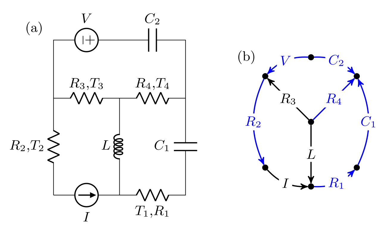
We consider circuits composed of two-terminal devices connected with each other forming a network. A given circuit is mapped to a connected graph in which each two-terminal device is represented by an oriented edge or branch (see Figure 1). The orientation of each edge serves as a reference to indicate voltages drops and currents in the standard way. The state of the circuit is specified by the nodes voltages and the edge currents , where is the number of nodes and is the number of edges. We consider five types of devices: voltage sources, current sources, capacitors, inductors and resistors. The charges of all capacitors and the magnetic fluxes of all inductors are the dynamical variables of the circuit (alternatively, the voltages and currents, respectively). In order for these variables to be truly independent, we consider circuits fulfilling the following two conditions11 1 A given circuit can always be made to satisfy conditions (i) and (ii) by adding small stray inductances or capacitances.: (i) The circuit graph has no loops22 2 A loop or cycle is a sequence of edges forming a path so that the first and last node coincide. formed entirely by capacitors and voltage sources, and (ii) The circuit graph has no cut-sets33 3 A cut-set or cocycle is a subset of edges such that their removal splits the graph into at least two disconnected parts. As a loop, it can be oriented, with the orientation indicating a prefered direction from one of the disconnected parts to the other. formed entirely by inductors and current sources. If condition (i) is fulfilled, then the voltages of all capacitors and voltage sources are independent variables, i.e., they cannot be directly related via the Kirchhoff’s voltage law (KVL). Analogously, if condition (ii) is fulfilled, then the currents of all inductors and current sources are independent variables since they are not directly constrained via the Kirchhoff’s current law (KCL).
The mathematical description of the circuit is easily constructed based on a tree of the circuit graph. A tree is a fully connected subgraph with no loops (see Figure 1-(b)). Under conditions (i) and (ii) it is always possible to find a tree for which all the edges corresponding to capacitors and voltage sources are part of the tree, and all the edges corresponding to inductors and current sources are out of it. We will call such a tree a normal tree and we will base our dynamical description of the circuit on it. Following the terminology of balabanian1969 we will refer to edges in the normal tree as twigs and edges outside it as links (also known as co-chords and chords, respectively). Thus, all capacitors and voltage sources are twigs, while all inductors and current sources are links. The edges corresponding to resistors can be split in two groups according to whether or not they are part of the normal tree. Every tree has twigs and therefore links.
II.1 Loops and cut-sets matrices
Given a set of oriented loops we define the loop matrix as follows:
| (1) |
A normal tree can be used to define a set of independent oriented loops in the following way: take the tree subgraph and add a link edge to it, then a loop will be formed (otherwise that link should have been a twig). The orientation of the loop is chosen to coincide with that of the added link. This can be done for every link. If we order the edges by counting first the twigs and then the links, the loop matrix thus obtained has the following structure:
| (2) |
where is the identity matrix. For the normal tree indicated in Figure 1-(b), the matrix is:
| (3) |
and specifies which twigs are involved in the loops corresponding to each link.
Given a set of oriented cut-sets (or cocycles) we define the cut-set matrix as:
| (4) |
As before, a normal tree can be used to define a set of independent cut-sets. The procedure is as follows. Take the tree subgraph and remove a twig, then the graph is split into two disconnected subgraphs. Consider all the edges going from one subgraph to the other, including the removed twig. These edges then form a cut-set which is oriented as the removed twig. This is then repeated for every twig, obtaining the following cut-set matrix:
| (5) |
With the same ordering as before, the matrix for the circuit of Figure 1 is:
| (6) |
and as we see specifies which links belong to the cut-set corresponding to a given twig. More details about the construction of the loop and cutset matrices can be found in Appendix A.
The matrices and are orthogonal in the sense that . This property follows naturally from their definitions and implies that . We also mention that loops and cut-sets can be identified algebraically from the incidence matrix of the graph, and that the loop and cut-set matrices satisfy additional algebraic relations polettini2015.
II.2 Kirchhoff’s Laws and Tellegen’s theorem
If and are column vectors with the edge current and voltage drops as components, respectively, then the Kirchhoff’s laws can be expressed in terms of the loop and cut-set matrices as follows:
| (7a) | ||||
| (7b) | ||||
These form a set of independent algebraic equations that can be used to eliminate half of the variables contained in and . In particular, if we order the components of and such that twig variables appear first, we can employ Eqs. (2) and (5) and write:
| (8a) | ||||
| (8b) | ||||
where and . We see then that it is enough to give the twigs voltages and the links currents to determine the rest of the variables.
From the orthogonality of and and the two Kirchhoff’s laws, it is possible to prove Tellegen’s theorem: any vector compatible with the KVL and any vector compatible with the KCL are orthogonal, i.e, .
II.3 Block structure of , and
In the following we will assume the previous splitting of the vectors and :
| (9) |
Also, since all voltage sources (E) and capacitors (C) are twigs, while all current sources (I) and inductors (L) are links, we can further split the vectors and as follows:
| (10) |
where stands for or and and indicate the resistive edges which are respectively twigs or links. This partitioning induces the following block structure in the matrix :
| (11) |
Thus, for example, each column of the block correspond to an inductive edge (which is a link) and its rows specify which capacitive edges (twigs) are involved in the cut-set corresponding to that inductive edge. For the matrix of Eq. (6), we have .
II.4 Constitutive relations
Each two-terminal device in the circuit is characterized by a particular relation between the electric potential difference across its terminals and the current through it. Voltage sources just fix a definite value for the potential difference, regardless of the current, and current sources fix a current value regardless of the voltage. Resistors are described by an algebraic relation between voltage and current. We can write,
| (12) |
where and are diagonal matrices with the resistances of the twigs and links resistors as non-zero elements, respectively. and can be time-dependent. Also, for non-linear resistors like diodes these matrices can also be functions of the voltages or currents.
Finally, capacitors and inductors are described by the following set of differential equations:
| (13) |
Here, and are symmetric matrices describing the capacitances and inductances of the circuit. is usually diagonal, but could account for cross-couplings between different inductors. As with resistors, they can also depend on time and/or describe non-linearities.
III Derivation of dynamical equations
We want to obtain an equation of motion for the circuit describing the evolution of the voltages of all capacitors and the currents in all inductors. We begin with the constitutive equations for them:
| (14) |
The task now is to use the Kirchhoff’s laws and the algebraic constitutive equations for the resistors to express the variables and in terms of the dynamical ones and . First, we use the following KCL and KVL equations which are parts of Eq. (7):
| (15a) | ||||
| (15b) | ||||
and we then obtain:
| (16) |
where we have defined the matrices , and (the subindices stand for conservative, sources and dissipation, as will be justified in the following). We now only need to eliminate and , since and are given. For this we use the constitutive relations of Eq. (12) and two additional Kirchhoff relationships:
| (17a) | ||||
| (17b) | ||||
which can be rewritten as:
| (18) |
where we have defined the additional matrices and (in this case the subindex stands for source dissipation). Inserting this relation in Eq. (16), a closed dynamical equation for the variables and is obtained. We can express it in the following concise form:
| (19) |
where the matrix coefficients are given by:
| (20) |
and
| (21) |
Note that might depend on time if resistances do. Some comments about the structure of the matrix are in order. The first term in Eq. (20), , describes the conservative interchange of energy between capacitors and inductors. In some cases it can be interpreted as analogous to the symplectic matrix in Hamiltonian mechanics. It has a block structure that stems from the separation of variables according to its behaviour under time reversal (voltages are even under time reversal while currents are odd). The second term takes into account the effect of the resistances in the dynamics. It is twofold: the antisymmetric part of describes the interchange of energy between capacitors and inductors that is allowed by resistive channels, and the symmetric part describes the loss of energy of those elements (see Eq. 27). Importantly, both the symmetric and antisymmetric part of respect the block structure of . The meaning of this property is that energy dissipation is bound to be an invariant quantity upon time reversal, and has important consequences regarding the non-equilibrium thermodynamic behaviour of the circuit, as discussed in more detail in Appendix C.
III.1 Charge and flux variables
Instead of working with and as dynamical variables, from a physical point of view it is more natural to work with the charges in the capacitors and the magnetic fluxes in the inductors. They are defined as and , respectively. We will group them in a column vector . Thus, we can write
| (22) |
where we have defined the matrix . With these definitions, the dynamical state equation now reads:
| (23) |
where is a vector grouping the voltage and currents of the sources, that can depend on time.
III.2 Linear energy storage elements
If we consider the particular case in which the matrices and , and thus also , do not depend on the state vector , we can express the energy contained in the circuit at a given time as a quadratic function of the circuit state:
| (24) |
Then, we can write the dynamical state equation as:
| (25) |
Note that Eq. (25) still allows for non-linear resistive relations, and in that case the matrices and have a tacit dependence on (through ).
III.3 Energy balance
We now analyze the balance of energy between the different elements of the circuit and the entropy produced during its operation. We consider linear storage elements since in this case we have a simple notion of energy associated to a given state of the circuit, which is given by Eq. (24). We begin by writing down the variation in time of the circuit energy:
| (26) |
We see that it naturally splits into tree distinct terms that account for different mechanisms via which the energy stored in capacitors and inductors can change. The first one describes how this energy is dissipated into the resistors. Note that only the symmetric part of plays a role in the expression , and from the definition of in Eq. (20), we see that it can only be different from zero if there are resistors in the circuit. Explicitly,
| (27) |
where indicates the symmetric part of . Secondly, voltage and current sources in the circuit can give energy to the capacitors and inductors, and this is described by the second term. Finally, external changes in the capacitances or inductances can also contribute to the circuit energy. This is clearly identified as work performed on the circuit by an external agent.
To complete the understanding of the energy balance of the circuit, we analyze the total rate of energy dissipation in the resistors (i.e, Joule heating). Thus, the instantaneous dissipated power in each resistor is , and the total rate of heat production reads:
| (28) |
Using Eq. (18) to eliminate the resistor currents and voltages we find:
| (29) |
As we will see next, the first term of the previous expression is exactly defined in Eq. (27), and thus represents the part of the energy dissipated into the resistors that is lost by capacitors and inductors. The second term corresponds to the part of the energy that is dissipated into the resistors directly by the voltage or current sources. The identity between and the first term of Eq. (29) can be established from the following property of the matrix :
| (30) |
that can be proven from the definition of via block matrix inversion. Using this, we can write the following expression for the energy balance of the circuit:
| (31) |
where the total work rate is the sum of the rates of work performed by the sources, , and by an external agent that drives the circuit parameters, . They are given by:
| (32) |
and
| (33) |
As expected, using the fact that and Tellegen’s theorem, we find that
| (34) |
III.4 Entropy production
At the level of description considered so far, the only aspect of entropy production that can be accounted for is the one related to the generation of heat in the resistors due to non-vanishing net currents. Thus, to every resistor we associate a instantaneous entropy production equal to , where is the temperature of the considered resistor. Therefore, we can write the total entropy production as
| (35) |
where is a diagonal matrix with the inverse temperatures of the resistors as non-zero elements. As with , Eq. (18) can be employed to express in terms of known quantities. However, we know in advance that the previous expression for entropy production is incomplete, since it doesn’t take into account the effects of fluctuations. There are three main ways or mechanisms via which the fluctuations can play a role. In general, if there are fluctuations then the state of the circuit and its evolution become stochastic. Therefore an entropy can be associated to the probability distribution of the state at any time, which will in general change and evolve in a non-trivial way. Of course, if the circuit is operating in a steady state this internal contribution to the total entropy production will vanish. But even in that situation fluctuations can still play a role, in combination with other two conditions. First, if the resistors are at different temperatures then fluctuations alone can transport heat from a hot resistor to a cold one ciliberto2013; ciliberto2013b, and this non-equilibrium process has an associated entropy production. Secondly, even if all the resistors are at the same temperature, heat transport can be induced by the driving of the circuit parameters delvenne2014. For example, it is possible to devise a cooling cycle in which two capacitors are used as a working medium to extract heat from a resistor and dump it into another resistor (see Section VI). In linear systems, this can be done only through fluctuations, without affecting the mean values of current and voltages and even in the case in which they vanish at all times. All these aspects of the full entropy production in linear circuits will be explored using stochastic thermodynamics in the next sections.
IV Stochastic dynamics
IV.1 Johnson-Nyquist noise
In this section we extend the previous description of RLC circuits to take into account the effects of the Johnson-Nyquist noise johnson1928; nyquist1928 originating in the resistors. To do so, we model a real resistor as a noiseless resistor connected in series with a random voltage source. The voltage of this source has zero mean, , and for high temperatures is modeled as delta correlated:
| (36) |
where is the resistance of the considered resistor, is its temperature, and is the Boltzmann constant. This corresponds to a flat noise spectrum . For low temperatures or high frequencies, one should instead consider the ‘symmetric’ schmid1982; clerk2010 quantum noise spectrum:
| (37) |
where is the Planck’s distribution. The 1/2 term added to the Planck’s distribution takes into account the environmental ground state fluctuations. It has no consequences regarding the thermodynamics of static circuits, even for non-equilibrium conditions. However, it does have important consequences in the ultralow temperature regime in the case of driven circuits, as discussed in detail in Section VII.4. In the following we will just consider the classical case of high temperatures and delta correlated noise, where simpler results hold and the usual machinery of stochastic calculus can be employed. Then we present in Section VII the full treatment of quantum noise using Green’s functions techniques.
IV.2 Langevin dynamics
Thus, if we want to consider Johnson-Nyquist noise in our general description of circuits we need to introduce a random voltage source with the previous characteristics for every resistor in the given circuit. This can be done directly by considering each voltage source as a new element in the circuit graph, or indirectly by taking into account the presence of the new voltage sources in the Kirchhoff’s laws of the original circuit. The latter approach has the advantage of not modifying the graph of the circuit and is the one we are going to use in the following. Thus, Eq. (15-b) becomes
| (38) |
and similar modifications to Eqs. (17) lead to the following generalization of Eq. (18):
| (39) |
where and are column vectors with the random voltage associated with links or twigs resistors, respectively. These modifications to the Kirchhoff’s laws are propagated straightforwardly to the final equation of motion in Eq. (25), which now reads:
| (40) |
where the vector groups the random voltages in the following way:
| (41) |
In what follows, for simplicity, we will omit the explicit dependence on time of , and , which are anyway constant if the resistances are also constant. The previous expression for the equation of motion can be cast into a slightly more symmetric form. For this we note that since the statistics of the noise variables are invariant under sign inversion we can neglect the minus sign in front of . Also, for high temperatures, taking into account the form of the spectrum for each random voltage we can write:
| (42) |
where is the matrix defined in Eq. (28), is the matrix of inverse temperatures defined in Eq. (35), and is a column vector of unit-variance white noise variables (as many as there are resistors). Then, the equation of motion for the circuit takes the following Langevin form:
| (43) |
where and are the same as in the deterministic case. The last sum is over every resistor in the circuit, and is given by
| (44) |
where is a projector over the one-dimensional subspace corresponding to resistor . Note that the matrices depend on time only if resistances do. Also, they always satisfy for . However the other possible product does not vanish in general. Eq. (43) is the stochastic generalization of the usual state equation for electrical circuits.
IV.3 Mean values and covariance matrix dynamics
For linear circuits, the mean values of the charges and fluxes evolve according to the deterministic equation of motion:
| (45) |
The evolution of the covariance matrix can be easily derived from the Langevin equation and reads:
| (46) |
It is important to note that for linear circuits the evolution of the covariance matrix is completely independent from the forcing function (if it is noiseless, as we considered). Thus, deterministic forcing of the circuit via voltage or current sources can only change the mean values of the charges and fluxes in the circuit, but not the fluctuations around them nor their correlations.
V Stochastic thermodynamics
V.1 Fluctuation-dissipation relation
We now consider the particular case in which the circuit is not driven (its parameters are time independent), all the resistors are at the same temperature , and no voltages or currents are applied (). Then, according to equilibrium thermodynamics the system must attain a thermal state for long times, with a distribution:
| (47) |
This is a Gaussian state with covariance matrix
| (48) |
It is instructive to check that in fact this result is obtained from the previous dynamical description of the circuit. Thus, if there is an asymptotic stationary state we see from Eq. (46) that in isothermal conditions its covariance matrix must satisfy
| (49) |
Also, using the definition of the matrices (Eq. (44)), we see that:
| (50) |
where in the second equality we used the previously mentioned property . Eq. (50) is nothing else that the fluctuation-dissipation (FD) relation for general RLC circuits. Using the FD relation, we can easily verify that the covariance matrix is in fact a solution of Eq. (49).
We finally note that, due to the linearity of the circuit, if the circuit is forced by constant voltages and/or current sources, then the asymptotic state is given by a displaced thermal state:
| (51) |
where the mean values are given by the stationary solution of Eq. (45). However, is not an equilibrium state since, at variance with , it has a non-vanishing entropy production given by Eq. (35).
V.2 Energy balance
To write down the energy balance for the stochastic description, we begin by noticing that since the energy is a quadratic function, its mean value can be easily expressed in terms of the mean values and the covariance matrix : . Therefore, we have
| (52) |
where is the energy function in Eq. (24). Thus, the energy balance takes the same form as before
| (53) |
with the following expressions for the driving work and heat terms:
| (54) |
and
| (55) |
where is the heat rate of Eq. (29). Finally, the work performed by the sources is equal to its deterministic value in Eq. (33) (for noiseless sources):
| (56) |
V.3 Local heat currents
Using Eq. (46) for and the FD relation of Eq. (50), we can rewrite Eq. (55) for the total heat dissipation rate as:
| (57) |
where for clarity we omitted the explicit time dependence of . We see that each term in the sum of the previous equation can be associated to a particular resistor in the circuit. Then, they are a sensible definition for the local heat currents (the rate of energy dissipation in resistor ):
| (58) |
This heuristic definition of the local heat currents is sometimes considered in the literature (see, for example, parrondo1996), but it is not always correct. In fact, if we add to the quantities defined in the previous equation a term of the form , for any antisymmetric tensor , we find that the total heat rate remains unchanged. Then, it is in general not possible to derive local heat currents via a decomposition of the global one.

From another perspective, in the context of electrical circuits the local heat currents can be naturally defined as
| (59) |
where is the random voltage associated to each resistor. That quantity, however, is found to be divergent in the general case. The physical origin for this divergence is the fact that for some circuits thermal fluctuations of arbitrarily high frequencies originating in a resistor (which are always present in the model due to the white-noise idealization) can be dissipated into another, as illustrated in Figure 2 with a simple example. There are two different reasons why this might happen. On one hand, the initial description of the circuit might be missing important degrees of freedom that are relevant for the thermodynamics, while still being valid from a purely dynamically point of view. This was recently discussed in celani2012; polettini2013; bo2014; murashita2016, in connection to the overdamped approximation in stochastic dynamics, even though not in the specific context of electrical circuits. In particular, in murashita2016 it was shown that when a particle is in simultaneous contact with multiple reservoirs at different temperatures there is a transfer of heat associated to its momentum degree of freedom at a rate that is inversely proportional to the relaxation timescale, which is taken to be infinitesimal in the overdamped limit (Figure 2-(b) is actually an example of this situation, as explained in the caption). On the other hand, heat currents might also be ill-defined independently of whether or not some kind of underdamped approximation was made in the description of the circuit. In those cases one should consider a more realistic model for the noise in the resistors, going beyond the white noise idealization. This is the more general way to address this issue, which is discussed in the next section.
From this discussion and the examples of Figure 2, we expect that the possibility to define finite heat currents in a given circuit is related to its topology. Indeed, this intuition is confirmed in the next section, where it is shown that the quantities , as defined in Eq. (59), are always well behaved if and only if, given a normal tree of the graph of the circuit, there are no fundamental cut-sets associated to it containing link resistors and twig resistors simultaneously (i.e, if in Eq. (11)). In that case, Eqs. (58) and (59) coincide.
V.4 Fokker-Planck equation for the circuit state and heat currents
Each resistor was modeled as an ideal resistor in series with a random voltage noise. If is the instantaneous current flowing through the resistor, then the rate of energy dissipation in it is
| (60) |
where is the voltage drop in the ideal resistor and is the random voltage. We want to express the quantity in terms of the state of this circuit. For this, we first write it as
| (61) |
where is the projector associated with the -th resistor appearing in Eq. (44), and is the matrix of resistances defined in Eq. (28). We can now use Eq. (39) to eliminate the variables and . For ease of notation, in the following we will not consider the terms associated to the sources of the circuit, as we know that they can only affect the mean values of the current and voltages and we are only interested in the stochastic contributions to the heat currents. In this way, after some manipulations, we obtain the following expression:
| (62) |
Notice that the last term in this expression is quadratic in the noise variables. As a consequence, it will give a divergent contribution to in the white noise limit, proportional to . As we already mentioned, the physical origin of this divergence is the possibility of direct heat transport at arbitrarily high frequencies between resistors at different temperatures. We stress that this problem only arises with regard to the definition of local heat currents, while the state of the circuit and the total heat rate are always well behaved quantities (see below). A solution to this problem would be to give a more realistic description of the resistive thermal noise, associating to each resistor a spectral density vanishing for large frequencies, such that its noise spectrum is given by . However, this is equivalent to appropriately ‘dressing’ a white-noise resistor with inductors and/or capacitors that can be considered part of the circuit44 4 This is fully analogous to well known ‘Markovian embedding’ techniques. (a capacitor in parallel or a inductor in series to a given resistor being the most simple options to filter out high frequencies, see Figure 2). This observation hints at a relationship between the topology of the circuit and the possibility of defining well behaved local heat currents. In fact, we see that the quadratic terms in the noise vanish if the matrix is block diagonal. In turn, from the definition of we can see that this happens if . Thus, is a sufficient condition for the local heat currents to be well behaved. In Appendix B it is shown that this condition is also necessary. We also show in the same Appendix that this condition can be restated in a way that does not make reference to any tree. To finish this discussion, we note that since and is always block diagonal (recall Eq. (30)), we see that the total heat rate is always well behaved in the white noise limit, even if .
Thus, assuming , the local heat currents are simplified to:
| (63) |
where is the vector of random voltages and currents defined in Eq. (42) and we used the fact that for we have . This equation is a Langevin equation for the heat that is of course coupled to the Langevin equation in Eq. (43) for the circuit state . Their integration is to be performed according to the Stratonovich procedure. As explained in gardiner2009 (Chapter 8), in the white noise limit the corresponding stochastic dynamics can be described by the following set of Ito differential equations:
| (64) |
and
| (65) |
where is a vector of independent Wiener processes differentials. Taking the mean value of Eq. (65) we recover Eq. (58) for . The Fokker-Planck equation for the joint probability distribution corresponding to the previous Ito differential equations reads:
| (66) |
where is the nabla operator with respect to the variables . The corresponding equation for the reduced probability distribution is just
| (67) |
Equation (66) allows to analyze the full statistics of the heat currents. Indeed, different integrated and detailed fluctuation theorems can be derived for this kind of linear and in general underdamped stochastic systems murashita2016; jakvsic2017; damak2019, valid for finite time protocols or asymptotic steady states. However, in this article we will focus only on the behaviour of the mean values.
V.5 Entropy production
We consider the continuous Shannon entropy
| (68) |
associated to the distribution and the total entropy production rate
| (69) |
Using Eq. (67) one can show that is non-negative:
| (70) |
where . Eq. (70) is the Second Law of thermodynamics for the circuit.
This total entropy production can be decomposed as a sum of adiabatic and non-adiabatic contributionsesposito2010; van2010; esposito2010pre; spinney2012, as shown in Appendix F. The adiabatic contribution is positive definite and for time independent circuits it is the only non vanishing contribution for large times. In general the non-adiabatic contribution can have any sign, but for overdamped circuits (for example, circuits with no capacitors or no inductors) it is also positive definite. If the circuit is time independent, then this contribution equals times the time derivative of the relative entropy between the instantaneous state and the stationary one (which for linear circuits is unique, although it might depend on the initial conditions). Thus, for time independent circuits is a always decreasing Lyapunov function. For underdamped circuits a third non-adiabatic term appears which, at variance with the previous two, is not positive definite. It is related to the change in due to a conservative flow in phase space, and vanish identically in isothermal conditions (when is an equilibrium state). These findings are analogous to the results of spinney2012.
VI A simple circuit-based machine
We now illustrate how our formalism can be used to design thermodynamic machines made of RLC circuits. External driving on the circuit allows to implement thermodynamical cycles that might extract work from a thermal gradient (non-autonomous heat engine), or extract heat from some resistors (non-autonomous refrigerator). We illustrate the basic techniques by considering a minimal circuit which can work both as an engine or a refrigerator. The circuit is shown in Figure 3 and consists of two parallel RC circuits coupled by an inductor. The capacitances in each RC circuit can be driven externally, for example by changing in time the distances between the plates of each capacitor, or, more practically, using varicap diodes. The circuit has no loops consisting only of capacitors or cutsets of all inductors, and therefore the previous formalism can be directly applied. We first analyze the simplest case of regular heat conduction for constant parameters and different temperatures. Then we show that the capacitances in the circuit can be driven in time in order to cool (i.e, extract heat) from one of the resistors, while dumping the extracted energy into the other one. Similar circuits were analyzed before in ciliberto2013; ciliberto2013b; karimi2016.

We begin by describing the circuit by the procedure of Section II. The state of the circuit is encoded in the vector , where is the charge in the capacitor and is the magnetic flux in . According to the edge orientations of Fig. 3-(b), the cutset matrix associated to the normal tree is specified by
| (71) |
and from this we can construct the matrix and :
| (72) |
Also, in this case and therefore:
| (73) |
Finally, we have , and .
VI.1 Heat conduction
Given the above matrices, we can readily solve Eq. (49) to find the stationary covariance matrix (for time independent parameters). The solution is particularly simple in the symmetric case in which and . It reads
| (74) |
where and . Similar results can be found in ciliberto2013; ciliberto2013b. Thus, the first term in the previous expression is just the equilibrium covariance matrix corresponding to the mean temperature . By examining the second term, we see that a temperature bias will establish correlations between the capacitors and the inductor, but not between the capacitors themselves. Since this circuit is not forced by voltage or current sources, the mean values of voltages and currents in any branch will vanish in the stationary state. Then, introducing the previous expression for the covariance matrix in Eq. (58) for the rate of heat dissipation in each resistor, we obtain:
| (75) |
where we have introduced the two characteristic timescales of the circuit, and , respectively associated to the dissipation rate and the free oscillations period. The entropy production can be computed from the above heat rates and reads:
| (76) |
Thus, in this case, the only dissipation in this circuit corresponds to static heat conduction from the hot to the cold reservoir.
VI.2 Cooling cycle
We now turn to analyze the more interesting situation in which the two resistors are at the same temperature and the capacitors are driven periodically in time such that and . Thus, both capacitances are driven with the same angular frequency and the same amplitude , but with some fixed phase difference . The matrices describing the circuit are the same as before except for the energy matrix that now depends on time. Since it is periodic, it can be decomposed as a Fourier series:
| (77) |
To lower order in we have only three Fourier components: and . We focus in regimes when a stable stationary state is reached. We note that this is not always the case due to the phenomenon of parametric resonance poulin2008. However, if there is a stable stationary state it will be such that the mean values of voltages and currents vanish, while the covariance matrix is periodic with the same period as the driving. Thus, we can decompose it as
| (78) |
Inserting the previous two Fourier decompositions into Eq. (46), we obtain an algebraic equation from which it is possible to obtain the coefficients in terms of and . This technique is explained in Appendix E. Once the Fourier components have been determined, we compute the average heat and work rates per cycle. Explicitly, we consider the quantity
| (79) |
where stands for , , or . We note that since the asymptotic state of the system is periodic. Thus, averaging the balance of energy (Eq. (31)) during a cycle we obtain
| (80) |
where is the average rate of work corresponding to the external driving, which is the only source of work in this case.
As shown in Appendix E, to lower order in and to second order in , is given by
| (81) |
while the average heat currents are
| (82) |
We then see that the rate of heat pumping from one resistor to the other (the first term in Eq. 82) is proportional to , while the rate at which work is performed by the driving (or equivalently, the total dissipated heat rate) scales as . Also, the pumping of heat is maximized and the dissipated work minimized for . This is natural since in this case the left/right asymmetry induced by the driving is maximum. The cooling efficiency or ‘Coefficient of Performance’ is
| (83) |
We note that in this isothermal case the CoP is not bounded by the Second law, and in fact diverges in the quasistatic limit . There is a maximum driving frequency such that cooling is not possible above it (in the considered regime of low and ). It corresponds to and for reads
| (84) |
There is also an optimal frequency , in the sense that the heat extracted from one of the resistors is maximized. We can obtain it by optimizing in Eq. (82) with respect to , and in this way we find that .
An intuitive understanding of how the cooling effect is achieved can be obtained by analyzing Eq. (58) for the heat currents. We note that the stochastic contribution is proportional to the difference between the energy contained in the circuit elements connected to a given resistor, and the energy they would have if they were in thermal equilibrium at the temperature of that resistor. For example, for the circuit of Figure 3, we have . Thus, we see that will be positive whenever the average energy contained in , , is larger that the corresponding to equilibrium, . Therefore, to achieve cooling of we require the variance to be, on average during a cycle, lower than its equilibrium value . This reduction in the variance in one degree of freedom with respect to its equilibrium value is the classical analogue to the well known concept of quantum squeezing rugar1991; natarajan1995. In quantum electronic and quantum optical setups, squeezing is a useful resource for metrology and it is usually achieved by means of some form of parametric driving yariv1967; anisimov2010; pirkkalainen2015; wollman2015. Here we see its additional role as a thermodynamic resource, which supports the already mentioned observation that parametric amplifiers can also be employed as refrigerators bergeal2010. Thus, an optimal cooling strategy is one in which a highly squeezed state is created and maintained in a dissipative and non-equilibrium environment. Finally, we mention that the methods of Appendix E can be employed to numerically optimize thermal cycles.
VI.3 Non-isothermal case
If the resistor temperatures are different the heat currents are
| (85) |
In contrast to the isothermal case, the term of second order in is too involved to be shown here. The first term corresponds to regular heat conduction in response to the thermal gradient. The second term is a correction to the regular heat conduction due to the driving, while the third term describes the pumping of heat. We consider the case in which (then, ) and analyze the conditions under which it is possible to extract heat from . The pumping of heat out of is, as before, optimized for . From the previous equation we see that in general the driving frequency must be above a minimum value in order for the heat pumping to overcome the heat conduction imposed by the thermal gradient. Thus, we will have effective cooling of only if . For this minimum cooling frequency reads
| (86) |
and we can write the heat rate as:
| (87) |
The previous considerations do not take into account the terms of second order in . From the expression of the heat currents in the isothermal case, Eq. (82), we know that these corrections correspond to heating and establish a maximum driving frequency such that cooling is not possible above it, Eq. (84). Thus, for cooling to be possible at all we need that , which imposes a condition on the temperature difference.
We now turn to analyze the total heat rate, or work rate. Up to second order in it is given by the following expression:
| (88) |
Note that that if then to lower order in the average work rate can be positive or negative, depending on the value of . This two cases correspond to the device working as a refrigerator or a (non-autonomous) heat engine, respectively. From Eqs. (87) and (88) it follows that the cooling efficiency in this case, to lower order in , is:
| (89) |
which is of course bounded by the Carnot efficiency .
VI.4 Exact numerical results
The previous analytical results for the cooling protocol are limited to low driving amplitude and frequency. In order to assess their validity in that regime and to study the behaviour of the system away from it, we numerically compute the heat currents. For this we integrate the differential equation for the time evolution of the covariance matrix (Eq. (46)). Then we compute the instantaneous expected values for the heat currents via Eq. (58), and obtain their averages during a cycle for sufficiently long times. For the numerical evaluation we consider and take this quantity as the unit of time. As an example we show in Figure 4-(a) the long time oscillations of the heat currents, as well as their averages, for an isothermal setting and the following driving parameters: , and the optimal phase difference of . The analytical and numerical results are compared in Figure 4-(b) for a fixed driving amplitude () and increasing driving frequency, while the temperatures are the same and the phase difference is the optimal. We see that the analytical expressions indeed match the numerical results in the low driving frequency regime. We also see that there is, as expected from the theoretical analysis, a maximum driving frequency such that both heat currents are positive if . However, the analytical results overestimate the value of . Analogously, we show in Figure 4-(c) the heat currents for fixed driving frequency () and increasing driving amplitude. Again, we see that for low driving amplitude the analytical expressions correctly describe the numerical results.
Finally, in Figure 5 we show the Coefficient of Performance as a function of the driving frequency for different values of . We see that cooling is possible only in a clearly defined range of driving frequencies. The lower limit of this range increases with , in accordance with Eq. (86), while the upper limit displays a weaker dependence on the same parameter. The points in each curve correspond to maximum cooling power, which is attained in all the cases at a frequency close to the optimal driving frequency of the isothermal case, . In all cases the maximum CoP is only about of the ideal value, . Thus, we see that this simple cooling scheme can only withstand small thermal gradients and operate at low efficiencies. More complex schemes are expected to improve these figures of merit, although they will probably share some of the properties of this elementary example, like the existence of minimum and maximum driving frequencies for cooling.
VII Quantum Johnson-Nyquist noise
We now turn to the low temperature regime of our theory. If the typical temperature in the circuit is low enough that the thermal energy starts to be comparable to the quantum of energy at the relevant frequencies , then the quantum nature of the noise in each resistor must be taken into account. One approach to work in this regime is to construct a quantum model of the circuit, assigning quantum mechanical operators to the charge and flux degrees of freedom in it (or a proper combination of them), satisfying the usual commutation relations. The dissipation and diffusion effects induced by the resistors are typically introduced using the Caldeira-Legget model for quantum Brownian motion caldeira1983. This is certainly the way to go if one is interested in having access to the full quantum state of the circuit (for modern treatments, see devoret1995; solgun2015; clerk2010; parra2019; burkard2004; girvin2011). However, this cannot be directly done for any circuit, since the canonical quantization procedure requires the detailed specification of stray or parasitic capacitances and inductances devoret1995. As an example we can take the overdamped circuit of Fig. 2-(c). This circuit has well behaved classical dynamics and heat currents, but cannot be directly quantized since it is missing inertial degrees of freedom. In other words, it is not possible to define canonical ‘momentum’ coordinates that are conjugate of the capacitor charges (there are no kinetic energy terms parra2019). To do that, one must give a more detailed description specifying stray inductances. Of course, any actual component in a real circuit is characterized by an impedance that is never purely resistive, capacitive or inductive. At a fundamental level we could consider elementary components which are always a combination of a single inductor and a single capacitor (resistors are then modeled as infinite arrays of them). Any circuit constructed in this way can be directly quantized, and based on this quantization the low temperature behaviour can be studied. Circuits like the one in Fig. 2-(c) result from having disregarded the inductive component in the impedance of the actual capacitors, which anyway might be an excellent approximation for practical purposes. However, this procedure of ignoring some degrees of freedom in the circuit is problematic, as we can see by considering the simple example of a series RLC circuit. The relevant frequency scales in this case are given by the dissipation rate , the oscillation frequency , and the thermal frequency . Under the high temperature condition , the equilibrium charge variance is and does not depend on . This justifies the use of an overdamped RC model, where the inductance is neglected compared to , in the high temperature regime. In contrast, if we take the overdamped limit for low temperatures we obtain that the equilibrium charge variance diverges as while the flux variance vanishes as (these scalings are obtained by keeping constant, otherwise we have and ). Thus, in general the covariance matrix of the circuit state is not well defined in this limit, and to compute it one needs to have precise information about the value of . In spite of this, we will see in the following that the heat currents are actually well defined in this kind of overdamped limits, and can be directly evaluated from the overdamped description of circuits even at low temperatures.
To show this we put forward a semiclassical approach that is based on the same stochastic equations of motion of Eq. (43), where now the noise variables are not white anymore and display a quantum spectrum. Then, if is the adimensional noise variable associated with the -th resistor, we must consider the following power spectrum:
| (90) |
where is the Planck’s distribution at temperature . Inverting the previous equation, we can compute the correlation functions:
| (91) |
where is a high-frequency cutoff, that must be large compared to any other frequency scale of the problem. The variables specifying the circuit state remain classical (they are not promoted to quantum mechanical operators). However, it is possible to show that for linear circuits that can be directly quantized, the results obtained in this way are fully equivalent to those obtained by a full quantization (under the Markovian approximation) schmid1982; freitas2017.
VII.1 Covariance matrix and heat currents for quantum noise
Since , for linear circuits the equation of motion for the mean values is still the fully deterministic one given in Eq. (45). However, in the quantum low temperature regime, the differential equation for the covariance matrix, Eq. (46), must be modified. The reason is that the circuit state at time will be in general correlated to (i.e, it will not be a non-anticipating function, and therefore the usual assumptions of stochastic calculus underlying the derivation of Eq. (46) are not valid gardiner2009). For stable systems it is still possible to obtain a simple expression for the covariance matrix at large times. To see this explicitly it is convenient to employ techniques based on the Green’s function of the circuit, like it is done in fully quantum mechanical models. We start with the equation of motion for :
| (92) |
Given the initial value , the solution to this equation can be written as
| (93) |
where the retarded Green’s function is defined as the solution of
| (94) |
with for (from this it follows that ). Then, the covariance matrix can be expressed as
| (95) |
The first term in this expression is just the deterministic evolution of the fluctuations present in the initial state. The second term takes into account the effect of the correlations between the circuit initial state and the environmental noise. The last term, which for stable systems dominates the long time behaviour, represents the diffusion induced by the environment. We will assume in the following that the initial state is not correlated in any way with the environmental noise, , and therefore the second term in the previous equation vanish. We will also assume, for simplicity, that the resistances, and thus the matrices and , are constant. Then, taking the time derivative of Eq. (95) and using Eq. (94), we obtain the following differential equation:
| (96) |
where is the convolution between the Green’s function and the correlation function of resistor :
| (97) |
Eq. (96) is the generalization for quantum noise of Eq. (46), which is recovered in the limit of high temperatures. To see this, we note that for high temperatures , and therefore .
Based on these results, we can now derive an expression for the local heat currents that, in contrast to Eq. (58), is exact and valid for arbitrary temperatures. In the quantum case the total heat rate is also given by Eq. (55): . However, this time we should replace by Eq. (96). Using this and the FD relation, we can write:
| (98) |
In analogy with the classical case, under the condition , we can identify the local heat currents as:
| (99) |
This expression can be evaluated using the above equations for and . However, if we are only interested in the asymptotic heat currents, under the assumption that the dynamics of the system is stable, we can express them as frequency integrals that might be easier to compute, and that also have a clear physical interpretation in terms of elementary transport processes.
VII.2 Asymptotic covariance matrix and heat currents
If the system is asymptotically stable, i.e, if for , then the first two terms in Eq. (95) can be neglected for sufficiently long times. By expressing the correlations in terms of the power spectrum via inversion of Eq. (90), we can rewrite the last term in Eq. (95) as:
| (100) |
where we have defined the following partial transform of the Green’s function:
| (101) |
For circuits that can be directly quantized, Eq. (100) is equivalent to what one obtains from a fully quantum model of the network and its environment under the Markovian approximation freitas2017.
If the circuit parameters are periodically driven, has the useful property of being asymptotically periodic in time with the same period as the driving, as shown in Appendix D. It also trivially satisfies , a property that is sometimes used implicitly in the derivations below. The convolution integral can also be expressed in terms of :
| (102) |
Finally, we note that can be directly obtained by solving its own evolution equation, that can be derived from Eq. (94) and reads
| (103) |
with the initial condition .
Introducing Eqs. (100) and (102) for and into Eq. (99), we can write the local heat currents as:
| (104) |
where we introduced the shorthand definition , that we will employ in the following to simplify the notation. The first term inside the trace, that is quadratic in , is actually closely related to the second one, which is linear in . We can see this by employing Eq. (103) to compute the derivative of :
| (105) |
Using this relationship and Eq. (50), it is possible to rewrite Eq. (104) in the following compact way:
| (106) |
where is a transfer function, specifying how the temperature of resistor affects the heat current of resistor . For it is always positive and is given by:
| (107) |
while the diagonal elements are determined by the following expression for the sum over the first index:
| (108) |
Equation (106) is the central result of this article. It is a fully general expression for the local heat currents valid for arbitrary temperatures and driving protocols. Although it has been derived based on Eq. (78), which is in principle only valid for circuit descriptions that can be quantized, nothing prevents the evaluation of Eqs. (106), (107) and (108) for general, overdamped circuits. In fact, as we show analytically in Appendix G, the overdamped limit of the transfer function for a underdamped circuit correctly matches the transfer function directly obtained from the corresponding overdamped circuit. Later this is also verified numerically for the cooling scheme of Section VI.
To clarify the physical interpretation of the previous expressions we analyze first the particular case of time independent circuits.
VII.3 Undriven circuits
If the matrix is time independent, then for sufficiently long times we have, from Eq. (103), (this is just the Laplace’s transform of the Green’s function evaluated at ). Then, asymptotically, the transfer functions are time independent and , so that . Also, in this case is symmetric under interchange of the indexes and . To see this it is necessary to consider the block structure of the matrix , that is inherited by the matrix , and of the matrices . This is discussed in detail in Appendix C, in connection with the invariant nature of the dissipation upon time inversion. Thus, using these properties we recover the usual Landauer-Büttiker expression for the heat currents rego1998; dhar2006; yamamoto2006:
| (109) |
From this equation, the quantity can be naturally interpreted as the rate at which an excitation with frequency between and is transported from resistor to . We note that the symmetry of the transfer function in the undriven case causes the heat currents to only depend on the differences . The 1/2 terms added to each Planck’s distribution cancel each other. However, this is not the case for driven circuits, where is not symmetric in general. In that case, the ground state fluctuations represented by the term are responsible for the dissipation of heat into the resistors due to the parametric driving even if all the temperatures are zero.
Thus, Eq. (106) can be considered as the generalization to arbitrary driving protocols of the Landauer-Büttiker formula for the static case, Eq. (109). In the following section, we provide simplified expressions for the transfer functions in the case where the external driving is periodic. They are useful for the numerical study of thermal cycles.
VII.4 Periodically driven circuits
We now consider the situation where the matrix is a periodic function of time, and therefore can be decomposed as a Fourier series:
| (110) |
where is the angular frequency of the driving. In this case, assuming stable dynamics and long times, the function is also periodic with the same period of the driving, as shown in Appendix D. Thus, the following decomposition holds asymptotically
| (111) |
Then, the asymptotic covariance matrix of the system and the heat currents are also periodic, with period . We thus consider the average values of the heat currents during a driving period, that we denote , as we did in the example of Section VI. They are given by
| (112) |
where is the asymptotic average of during a driving period, that can be expressed in terms of the Fourier components and :
| (113) |
for , and
| (114) |
Finally we note that, given the Fourier components of the external driving, the Fourier components of the Green’s function can be found by solving the following infinite set of algebraic equations
| (115) |
that is obtained by introducing the decompositions of Eqs. (110) and (111) into Eq. (103). Some methods to solve this equation are discussed in Appendix D.
The interpretation of the previous expressions in terms of elementary transport processes is not as straightforward as in the regular Landauer-Büttiker formula for the undriven case. For open mechanical systems composed of quantum harmonic oscillators, a physically clear decomposition of the local heat currents in terms of assisted transport and pair creation of excitations was obtained recently freitas2017. In particular, the pair creation mechanism was shown to be dominant at low temperatures and to be responsible for the ultimate limit for cooling in those systems. In the next section, this quantum limit for cooling is illustrated numerically for the cooling scheme introduced in Section VI.
VII.5 Quantum limits for cooling

In this section we explore the low temperature behaviour of the heat currents for the cooling scheme of Section VI. We show how the quantum corrections to the heat currents impose a minimum temperature below which it is not possible to extract heat. Also, this will serve us to show that the overdamped description of circuits can be directly employed to compute the heat currents in the low temperature regime.
We consider the particular cooling scheme of Section VI in isothermal conditions. Thus, both resistors are at the same temperature , and we choose a driving amplitude , frequency , and phase difference such that for high temperatures heat is extracted from resistor (thus, ), while it is dumped in resistor (). The heat currents are computed by evaluating Eqs. (112), (113) and (114), based on the overdamped circuit of Figure 3. In Figure 6-(a) we compare the classical (i.e, high temperature) heat currents, obtained by averaging Eq. (58) over a driving period, with the quantum heat currents according to Eq. (112). The parameters are , and (recall that and are the oscillation and dissipation time scales, respectively). As expected, the quantum heat currents approach the classical ones for increasing temperature. However, below a given value of (indicated as in Fig. 6-(a)), becomes positive and cooling stops. This is shown in more detail in Figure 6-(b), where it is also clear that the value of decreases with increasing , or equivalently with decreasing dissipation rate (In this case is selected as the optimal driving frequency for each value of ). This breakdown of the cooling effect is a strong coupling result that cannot be captured with usual approaches based on master equations (see karimi2016, for example), as discussed in detail in freitas2017. All these results are independent of the cutoff frequency for large .
In figure 6-(b) we also show the results obtained based on the circuit of Figure 7, for (indicated by crosses). This circuit can be considered an extension of the one in Figure 3 in which the additional stray inductance was specified. As shown in more detail in figure 6-(c), the heat currents obtained from the two descriptions match as . Thus, while overdamped descriptions of circuits are not enough to construct a quantum model and compute the quantum state, they are sufficient to compute the quantum corrections to the heat currents.
VIII Conclusions
We presented a general study of the non-equilibrium thermodynamics of driven electrical circuits. We derived the stochastic evolution of the circuit state and of the heat currents dissipated in each resistor. A relation between the topology of the circuit and the possibility of defining finite heat currents under the white noise idealization was established. As a first and simple example of application, we showed how to use our formalism to study the transport and pumping of heat in a minimal circuit of two driven RC circuits coupled by an inductor.
The initial classical treatment was then generalized in order to consider the effects of quantum low-temperature noise. We considered a semiclassical treatment in which the classical equations of motion are driven by noise with a quantum spectrum. In contrast with treatments based on the full quantization of the degrees of freedom in the circuit, our method has the advantage of being directly applicable to circuits that cannot be quantized without the additional specification of stray inductances or capacitances, but are however detailed enough to properly describe the dynamics and also the thermodynamics. Based on these results we expressed the heat currents for static circuits in terms of the familiar Landauer-Büttiker formula, and also obtained the generalization of this expression for arbitrary driving protocols.
Our results offer a general formalism to study and design thermodynamical processes in electrical systems from a first principles perspective and working in strongly non-equilibrium conditions, and also away from the adiabatic and weak coupling regimes. A direct application of the expressions provided and of the techniques illustrated in this article is the automatic optimization of thermal cycles in complex and large electrical circuits. This is particularly straightforward in the regime of high temperatures, where optimal cycles can be obtained that could be later refined to take into account quantum effects.
Finally, nontrivial networks with stochastic linear dynamics are commonly used to describe various kinds of complex systems including biological ones gnesotto2019; mura2018. In principle any such network can be emulated by a suitable RLC circuit. This means that not only our results may apply to a very broad class of systems, but also that experimental studies of those models could be carried out using RLC circuits.
IX Acknowledgments
We acknowledge funding from the European Research Council project NanoThermo (ERC-2015-CoG Agreement No. 681456).
References
- [1] Laszlo B Kish. End of moore’s law: thermal (noise) death of integration in micro and nano electronics. Physics Letters A, 305(3-4):144–149, 2002.
- [2] Udo Seifert. Stochastic thermodynamics, fluctuation theorems and molecular machines. Reports on progress in physics, 75(12):126001, 2012.
- [3] Riccardo Rao and Massimiliano Esposito. Conservation laws shape dissipation. New Journal of Physics, 20(2):023007, 2018.
- [4] R Van Zon, S Ciliberto, and EGD Cohen. Power and heat fluctuation theorems for electric circuits. Physical review letters, 92(13):130601, 2004.
- [5] Nicolas Garnier and Sergio Ciliberto. Nonequilibrium fluctuations in a resistor. Physical Review E, 71(6):060101, 2005.
- [6] Sergio Ciliberto, Alberto Imparato, Antoine Naert, and Marius Tanase. Heat flux and entropy produced by thermal fluctuations. Physical review letters, 110(18):180601, 2013.
- [7] Jukka P Pekola. Towards quantum thermodynamics in electronic circuits. Nature Physics, 11(2):118, 2015.
- [8] Norman Balabanian, Sundaram Seshu, and Theodore A Bickart. Electrical network theory. 1969.
- [9] Charles A Desoer. Basic circuit theory. Tata McGraw-Hill Education, 2010.
- [10] Antonio Celani, Stefano Bo, Ralf Eichhorn, and Erik Aurell. Anomalous thermodynamics at the microscale. Physical review letters, 109(26):260603, 2012.
- [11] Matteo Polettini. Diffusion in nonuniform temperature and its geometric analog. Physical Review E, 87(3):032126, 2013.
- [12] Stefano Bo and Antonio Celani. Entropy production in stochastic systems with fast and slow time-scales. Journal of Statistical Physics, 154(5):1325–1351, 2014.
- [13] Yûto Murashita and Massimiliano Esposito. Overdamped stochastic thermodynamics with multiple reservoirs. Physical Review E, 94(6):062148, 2016.
- [14] Aashish A Clerk, Michel H Devoret, Steven M Girvin, Florian Marquardt, and Robert J Schoelkopf. Introduction to quantum noise, measurement, and amplification. Reviews of Modern Physics, 82(2):1155, 2010.
- [15] Chris Macklin, K O’Brien, D Hover, ME Schwartz, V Bolkhovsky, X Zhang, WD Oliver, and I Siddiqi. A near–quantum-limited josephson traveling-wave parametric amplifier. Science, 350(6258):307–310, 2015.
- [16] AO Niskanen, Y Nakamura, and Jukka P Pekola. Information entropic superconducting microcooler. Physical Review B, 76(17):174523, 2007.
- [17] N Bergeal, R Vijay, VE Manucharyan, I Siddiqi, RJ Schoelkopf, SM Girvin, and MH Devoret. Analog information processing at the quantum limit with a josephson ring modulator. Nature Physics, 6(4):296, 2010.
- [18] Albert Schmid. On a quasiclassical langevin equation. Journal of Low Temperature Physics, 49(5-6):609–626, 1982.
- [19] Nahuel Freitas and Juan Pablo Paz. Fundamental limits for cooling of linear quantum refrigerators. Physical Review E, 95(1):012146, 2017.
- [20] Matteo Polettini. Cycle/cocycle oblique projections on oriented graphs. Letters in Mathematical Physics, 105(1):89–107, 2015.
- [21] Sergio Ciliberto, Alberto Imparato, Antoine Naert, and Marius Tanase. Statistical properties of the energy exchanged between two heat baths coupled by thermal fluctuations. Journal of Statistical Mechanics: Theory and Experiment, 2013(12):P12014, 2013.
- [22] Jean-Charles Delvenne and Henrik Sandberg. Finite-time thermodynamics of port-hamiltonian systems. Physica D: Nonlinear Phenomena, 267:123–132, 2014.
- [23] John Bertrand Johnson. Thermal agitation of electricity in conductors. Physical review, 32(1):97, 1928.
- [24] Harry Nyquist. Thermal agitation of electric charge in conductors. Physical review, 32(1):110, 1928.
- [25] Juan MR Parrondo and Pep Español. Criticism of feynman’s analysis of the ratchet as an engine. American Journal of Physics, 64(9):1125–1130, 1996.
- [26] Crispin Gardiner. Stochastic methods, volume 4. springer Berlin, 2009.
- [27] V Jakšić, C-A Pillet, and Armen Shirikyan. Entropic fluctuations in thermally driven harmonic networks. Journal of Statistical Physics, 166(3-4):926–1015, 2017.
- [28] Mondher Damak, Mayssa Hammami, and Claude-Alain Pillet. A detailed fluctuation theorem for heat fluxes in harmonic networks out of thermal equilibrium. arXiv preprint arXiv:1905.03536, 2019.
- [29] Massimiliano Esposito and Christian Van den Broeck. Three detailed fluctuation theorems. Physical review letters, 104(9):090601, 2010.
- [30] Christian Van den Broeck and Massimiliano Esposito. Three faces of the second law. ii. fokker-planck formulation. Physical Review E, 82(1):011144, 2010.
- [31] Massimiliano Esposito and Christian Van den Broeck. Three faces of the second law. i. master equation formulation. Physical Review E, 82(1):011143, 2010.
- [32] Richard E Spinney and Ian J Ford. Entropy production in full phase space for continuous stochastic dynamics. Physical Review E, 85(5):051113, 2012.
- [33] Bayan Karimi and JP Pekola. Otto refrigerator based on a superconducting qubit: Classical and quantum performance. Physical Review B, 94(18):184503, 2016.
- [34] Francis J Poulin and Glenn R Flierl. The stochastic mathieu’s equation. Proceedings of the Royal Society A: Mathematical, Physical and Engineering Sciences, 464(2095):1885–1904, 2008.
- [35] D Rugar and P Grütter. Mechanical parametric amplification and thermomechanical noise squeezing. Physical Review Letters, 67(6):699, 1991.
- [36] Vasant Natarajan, Frank DiFilippo, and David E Pritchard. Classical squeezing of an oscillator for subthermal noise operation. Physical review letters, 74(15):2855, 1995.
- [37] Amnon Yariv. Quantum electronics. Wiley, 1967.
- [38] Petr M Anisimov, Gretchen M Raterman, Aravind Chiruvelli, William N Plick, Sean D Huver, Hwang Lee, and Jonathan P Dowling. Quantum metrology with two-mode squeezed vacuum: parity detection beats the heisenberg limit. Physical review letters, 104(10):103602, 2010.
- [39] J-M Pirkkalainen, Erno Damskägg, Matthias Brandt, Francesco Massel, and Mika A Sillanpää. Squeezing of quantum noise of motion in a micromechanical resonator. Physical Review Letters, 115(24):243601, 2015.
- [40] Emma Edwina Wollman, CU Lei, AJ Weinstein, J Suh, A Kronwald, F Marquardt, Aashish A Clerk, and KC Schwab. Quantum squeezing of motion in a mechanical resonator. Science, 349(6251):952–955, 2015.
- [41] Amir O Caldeira and Anthony J Leggett. Path integral approach to quantum brownian motion. Physica A: Statistical mechanics and its Applications, 121(3):587–616, 1983.
- [42] Michel H Devoret et al. Quantum fluctuations in electrical circuits. Les Houches, Session LXIII, 7(8), 1995.
- [43] Firat Solgun and David P DiVincenzo. Multiport impedance quantization. Annals of physics, 361:605–669, 2015.
- [44] A Parra-Rodriguez, IL Egusquiza, DP DiVincenzo, and E Solano. Canonical circuit quantization with linear nonreciprocal devices. Physical Review B, 99(1):014514, 2019.
- [45] Guido Burkard, Roger H Koch, and David P DiVincenzo. Multilevel quantum description of decoherence in superconducting qubits. Physical Review B, 69(6):064503, 2004.
- [46] Steven M Girvin. Circuit qed: superconducting qubits coupled to microwave photons. Quantum Machines: Measurement and Control of Engineered Quantum Systems, page 113, 2011.
- [47] Luis GC Rego and George Kirczenow. Quantized thermal conductance of dielectric quantum wires. Physical Review Letters, 81(1):232, 1998.
- [48] Abhishek Dhar and Dibyendu Roy. Heat transport in harmonic lattices. Journal of Statistical Physics, 125(4):801–820, 2006.
- [49] Takahiro Yamamoto and Kazuyuki Watanabe. Nonequilibrium green’s function approach to phonon transport in defective carbon nanotubes. Physical review letters, 96(25):255503, 2006.
- [50] Federico S Gnesotto, Benedikt M Remlein, and Chase P Broedersz. Nonequilibrium dynamics of isostatic spring networks. Physical Review E, 100(1):013002, 2019.
- [51] Federica Mura, Grzegorz Gradziuk, and Chase P Broedersz. Nonequilibrium scaling behavior in driven soft biological assemblies. Physical review letters, 121(3):038002, 2018.
Appendix A Construction of the loop and cutset matrices
In this section we give a detailed explanation of how the loop and cutset matrices are constructed for the example of Figure 1-(a). The fist step is to identify a normal tree of the circuit graph (one possible normal tree is indicated in blue in Figure 1-(b)). By definition, all the capacitors and voltage sources should be part of the normal tree, while all inductors and current sources should be out of it. Also, as any tree, it cannot contain loops, and all the nodes should be connected. Thus, the edges , and should be part of the normal tree, while the edges and should be out of it. To identify the edges , , , and , we see that should be part of the tree, since otherwise the node at which arrives would be disconnected. should also be part of the tree, since otherwise the node from which departs would remain disconnected. Thus, and are twigs. Finally, and cannot be both part of the tree, since in that case they would form a loop with and . They also cannot be both outside the tree, since in that case the central node from which departs would be disconnected. Thus, one of them should be a twig and the other a link. We are free to choose between the two possible options, and in the example of Figure 1-(b) we have choosen as a twig.
Having identified the normal tree, we now proceed to construct the matrices of fundamental loops and cutsets associated to it. We begin with the loops. We can associate a loop to each link. For example, if we add link to the normal tree, then a loop if formed by the edges , , and (See figure 8).

The orientation of the loop is defined to be that of the added link, in this case , which matches the orientation of and , but is contrary to that of . The row corresponding to this loop in the full loop matrix is then:
| (116) |
The rows corresponding to the links and are constructed analogously. By adding link to the normal tree a loop is formed involving the twigs , , , and . Adding link we form a loop with twigs , and . All the loops are shown in Figure 8. Taking into account their orientations, the final full loop matrix is:
| (117) |
We see that the first block is just the identity, and the rest of the matrix is what is denoted by in the main text.
The construction of the cutset matrix is done as follows. A cutset can be associated to each twig. For example, if we remove twig , then the start and end nodes of are disconnected from the others (in the tree, not in the full graph). So we consider the splitting of the set of nodes in two subsets: the two nodes connected to , and all the rest. The edges going from one subset to the other are , , and of course (see Figure 9-(a)).

We give to this cutset the same orientation as , which happens to be contrary to the orientation of and . Then, the row corresponding to this particular cutset in the full cutset matrix is:
| (118) |
The other rows corresponding to the twigs , , , and are constructed in the same way. As an additional example, we note that removing twig from the normal tree we isolate the central node, and the corresponding cutset is formed by , and , which share the same orientation, as shown in Figure 9-(b). Adding the corresponding row to the previous one we have:
| (119) |
Filling in the remaining 4 rows to obtain the full cutset matrix, we find that the first block is the identity, and the remaining block is the one denoted by in the main text.
Appendix B Necessary and sufficient condition to have well defined local heat currents for white noise resistors
The matrix appearing in the last line of Eq. (62) has the following block structure:
| (120) |
The explicit form of each block can be derived from the definition of and using block matrix inversion. Using this, we see that the mean value of the last term in Eq. (62) can be written as:
| (121) |
where and are diagonal matrices with the temperatures of the link and twig resistors, respectively. For the previous expression to vanish for arbitrary temperatures, the matrices and should have null diagonals. The explicit form of is if the index correspond to a twig resistor, or if correspond to a link resistor, where is the reduction of the projector to the appropriate twigs or links subspace. In any case, it is easy to see that for the matrix to have null diagonal for any and for arbitrary values of the resistances, all the components of the matrix should vanish.
The condition means that there are no fundamental cutsets associated to the normal tree containing simultaneously a link resistor and a twig resistor. However, since it is ultimately related to the possibility of defining finite heat currents, its validity should be independent of the choice of normal tree. In fact, it is possible to obtain the following equivalent condition that does not make any reference to a particular tree of the graph:
- •
Given the full graph of the circuit, remove the I and L edges.
- •
Merge the connected components formed by E and C edges into a single node (this will remove internal edges, that might be resistors).
- •
The heat currents are finite if and only if the resulting network of only R edges is acyclic.
The equivalence with the condition is given by the following two observations: i) if there is a cycle in the final R network, then any normal tree will have a fundamental cutset involving a resistor in the tree and a resistor outside it, ii) if there is no cycle in the final R network, then all the edges in it will be part of any normal tree, and the fundamental cutsets associated to them will not involve any of the previously eliminated resistors (if any was eliminated).
Appendix C Block structure of the matrix and the invariance of dissipation upon time inversion
In this section, we show explicitly how the block structure of the matrix is related to the invariance of the dissipation upon time reversal and to the symmetry property of the transfer function involved in the expression for the heat currents for undriven circuits. We first recall the necessary definitions:
| (122) |
| (123) |
and
| (124) |
Using block matrix inversion, we see that has also a block structure like its inverse. Then it is straightforward to see that the matrix can be written as:
| (125) |
where and are symmetric matrices with dimensions and , respectively ( is the number of capacitors and the number of inductors). Therefore, the rate of energy dissipation is
| (126) |
where in the second line we introduced the block structure of the matrix and the state vector . Thus, we see that due to the block structure of the symmetric part of , the rate of energy dissipation has no cross terms coupling charges and fluxes . Therefore it is an even quantity under time reversal.
We now turn to discuss the symmetry of the transfer function for undriven circuits upon the interchange of and . This function is given by (Eq. (107) in the main text):
| (127) |
with . We first note that since is a positive definite matrix we can write the product in the more symmetric form , and thus we see that if were symmetric or antisymmetric, then the matrix would inherit that property. In any of those cases the function
| (128) |
would be trivially symmetric upon . However, has no definite symmetry. It has, nevertheless, a block structure that is also inherited by :
| (129) |
where the dimensions of , and are the same as , and in Eq. (125). If and are the symmetric and antisymmetric part of , we have
| (130) |
were we omitted the dependences in . Finally from the definitions of the matrices it can be seen that their products are block diagonal whenever , which is the condition for the heat currents to be properly defined in the white noise or high temperatures limit. From this it follows that the two last traces in the previous equation are zero, since their arguments have null diagonals. The remaining terms are easily shown to be invariant upon .
Appendix D Periodic driving
In this section we show some useful properties of the Green’s function of periodically driven and stable circuits. We begin with the expression for the transform given in Eq. (101):
| (131) |
Here, is the solution to
| (132) |
with for . If is a periodic function with period , and the solution to the previous differential equation is unique, then we have that . Then:
| (133) |
where in the first step we just employed a change of variables (), and in the last step we assumed that the system is stable, in the sense that for . If that condition holds, then for sufficiently large we can neglect the contribution of the first part of the integration domain. Thus, we have shown that under this condition the function is asymptotically periodic, with period . We note that the stability condition does not always hold, even in the presence of strong dissipation, since it is possible for the circuit to continuously absorb energy from the driving and have a divergent dynamics. This is the phenomenon of parametric resonance, that we exclude from our analysis.
Therefore, for long times we can give the following Fourier decomposition of the function :
| (134) |
Then, inverting Eq. (131) and using Eq. (132) (or equivalently, transforming Eq. (132) to obtain Eq. (103) in the main text), we can find the following set of algebraic equations for the coefficients :
| (135) |
A simple method to solve these equations is to use a perturbative approach in which the strength of the driving is considered small, i.e, we assume for all . Then, to first order in we have , that is just the transform of the Green’s function on the undriven circuit, and:
| (136) |
Higher orders in can be easily computed. From this solution, we see that for weak driving the range of relevant Fourier components in is restricted by that of . Thus, another non-perturbative method to solve Eq. (135) is just to truncate the Fourier space to some maximum number of components given by and and then numerically solve the resulting finite system of linear equations for each value of .
Appendix E Generalized Lyapunov Equation
In this section we introduce a generalization of the Lyapunov equation that is useful to compute the asymptotic state of periodically driven linear systems subjected to white noise. For undriven circuits, the covariance matrix for large times can be obtained as the solution of the following Lyapunov equation:
| (137) |
For driven circuits there is no time-independent asymptotic state and one must solve the dynamical equation:
| (138) |
However, if the function is periodic, then we known from the results of the previous section that the system state for large times will also be periodic (with the same period of ). Then we consider and introduce the following decomposition for :
| (139) |
Thus, the problem is now to find the coefficients in terms of . Note that, at variance with a regular Fourier decomposition, the previous expression involves a double summation and as a consequence the coefficients are not uniquely defined. This choice, however, allows to cast our problem as an extended Lyapunov equation. Indeed, it is useful to introduce the following definitions:
| (140) |
| (141) |
and
| (142) |
Then, it can be seen that the coefficients that give a solution to Eq. (138) can be obtained by solving the following generalized Lyapunov equation:
| (143) |
Of course, to numerically solve this problem we need to truncate the dimensions of the matrices and . As we saw in the previous section, this is justified for sufficiently weak driving. In the example given in Section VI, the function has only Fourier components, and therefore to lower order in we can truncate the matrix to blocks in each direction. After doing, this we solved symbolically the Lyapunov equation of Eq. 143 using Mathematica.
Appendix F Adiabatic and non-adiabatic decomposition of the entropy production
The Fokker-Planck equation for the circuit state can be cast as
| (144) |
where the total probability current was split into conservative and dissipative parts, that are respectively given by
| (145) |
and
| (146) |
where and are the symmetric and antisymmetric parts of . The total entropy production rate is:
| (147) |
with . Using the FD relation the dissipative probability current can be expressed in terms of the functions as follows:
| (148) |
For a given instantaneous value of , we define the corresponding steady state distribution as the one for which . It is the probability distribution to which the circuit would eventually relax if the parameters are frozen at the values given by . The functions corresponding to are denoted as . Then, by replacing in Eq. (147), we obtain the following decomposition of the total entropy production:
| (149) |
where
| (150) |
| (151) |
with , and finally
| (152) |
The terms and vanish in the adiabatic limit of infinitely slow driving, since the state is always the stationary one and . For the same reason they vanish for long times if there is no driving. In contrast, converges to the entropy production in the stationary state, which is . The non-adiabatic (nad) terms can be interpreted in terms of the relative entropy of the instantaneous state with respect to the stationary state. Indeed, can be expressed as:
| (153) |
and therefore in the absence of external driving ( and therefore are constants) it equals times the derivative of the relative entropy . The term also accepts the following expressions:
| (154) |
and can therefore be interpreted as a the change in the relative entropy due to the conservative flow in phase space. At variance with , is not always positive. It vanishes identically in the following cases: i) for circuits with no inductors or no capacitors (in that case we can consider and the dynamics is always overdamped), and ii) in isothermal conditions, since the steady state satisfies and therefore . Finally, adding the last two equations and using Eq. (144), we can see that the sum of the non-adiabatic terms only depends on the dissipative current:
| (155) |
We note that this quantity is not necesarily positive definite. It is positive for overdamped circuits, since we have seen that in that case and .
Appendix G Underdamped limit for static heat conduction

In this section we illustrate with an example how the heat transfer function of an overdamped circuit is recovered by taking the appropiate limit in the heat transfer function of a underdamped circuit. We consider the circuit in Figure 10-(a), that in the limit reduces to the circuit of Figure 2-(c) in the main text.
We consider the heat transfer function given by Eq. (107) in the main text (only the non-diagonal element is necessary in this case of stationary heat conduction):
| (156) |
where
| (157) |
The matrices , and for each circuit are to be constructed according to the procedure of Section II in the main text. In this way, we obtain the following transfer function for the circuit of Figure 10-(a):
| (158) |
and for the circuit of Figure 10-(b):
| (159) |
Thus, a simple calculation shows that in fact
| (160) |