跳到论文正文
W Papers独立论文阅读器 arXiv:1906.11008 论文正文 计算阅读时间 · 0%
引用这篇论文根据当前论文元数据生成,正式投稿前建议核对。


License: CC BY-SA 4.0
arXiv:1906.11008v2 [math.NA] 10 Nov 2019

A registration method for model order reduction: data compression and geometry reduction

Abstract

We propose a general — i.e., independent of the underlying equation — registration method for parameterized model order reduction. Given the spatial domain Ω⊂ℝd\Omega\subset\mathbb{R}^{d} and the manifold ℳu={uμ:μ∈𝒫}\mathcal{M}_{\rm u}=\{u_{\mu}:\mu\in\mathcal{P}\} associated with the parameter domain 𝒫⊂ℝP\mathcal{P}\subset\mathbb{R}^{P} and the parametric field μ↦uμ∈L2​(Ω)\mu\mapsto u_{\mu}\in L^{2}(\Omega), the algorithm takes as input a set of snapshots {uk}k=1ntrain⊂ℳu\{u^{k}\}_{k=1}^{n_{\rm train}}\subset\mathcal{M}_{\rm u} and returns a parameter-dependent bijective mapping 𝚽:Ω×𝒫→ℝd\boldsymbol{\Phi}:\Omega\times\mathcal{P}\to\mathbb{R}^{d}: the mapping is designed to make the mapped manifold {uμ∘𝚽μ:μ∈𝒫}\{u_{\mu}\circ\boldsymbol{\Phi}_{\mu}:\,\mu\in\mathcal{P}\} more suited for linear compression methods. We apply the registration procedure, in combination with a linear compression method, to devise low-dimensional representations of solution manifolds with slowly-decaying Kolmogorov NN-widths; we also consider the application to problems in parameterized geometries. We present a theoretical result to show the mathematical rigor of the registration procedure. We further present numerical results for several two-dimensional problems, to empirically demonstrate the effectivity of our proposal.

Tommaso Taddei1

1 IMB, UMR 5251, Univ. Bordeaux; 33400, Talence, France. Inria Bordeaux Sud-Ouest, Team MEMPHIS; 33400, Talence, France, tommaso.taddei@inria.fr

Keywords: parameterized partial differential equations; model order reduction; data compression; geometry registration.

1 Introduction

1.1 Background

Numerical simulations based on mathematical models represent a valuable tool to study complex phenomena of scientific interest and/or industrial value. For several applications — including design and optimization, uncertainty quantification, active control — it is important to approximate the solution (and associated quantities of interest) to the model over a range of parameters: parameters might correspond to material properties, geometric features, operating conditions. To alleviate the computational burden associated with the evaluation of the model for many values of the parameters, parameterized model order reduction (pMOR) techniques aim to generate a reduced-order model (ROM) that approximates the original system over a prescribed parameter range. In this work, we shall develop a general — i.e., independent of the underlying equation — registration procedure for pMOR applications; we shall here focus on systems modelled by stationary partial differential equations (PDEs). In computer vision and pattern recognition, registration refers to the process of finding a spatial transformation that aligns two datasets; in this paper, registration refers to the process of finding a parametric transformation that improves the linear compressibility of a given parametric manifold.

We denote by μ\mu the set of parameters associated with the model in the prescribed parameter domain 𝒫⊂ℝP\mathcal{P}\subset\mathbb{R}^{P}; we denote by Ω⊂ℝd\Omega\subset\mathbb{R}^{d} (d=2,3d=2,3) the spatial domain, which is assumed to be Lipschitz; we also introduce the Hilbert space 𝒳\mathcal{X} defined over Ω\Omega, endowed with the inner product (⋅,⋅)(\cdot,\cdot) and the induced norm ∥⋅∥:=(⋅,⋅)\|\cdot\|:=\sqrt{(\cdot,\cdot)}. Then, we introduce the problem:

find​𝐲μ:=𝔰μ​(zμ)​s.t.𝒢μ​(zμ,v)=0​∀v∈𝒳,{\rm find}\;\mathbf{y}_{\mu}:=\mathfrak{s}_{\mu}(z_{\mu})\;\;{\rm s.t.}\;\;\mathcal{G}_{\mu}(z_{\mu},v)=0\;\;\forall\,v\in\mathcal{X}, (1)

where 𝐲μ\mathbf{y}_{\mu} is a vector of DD quantities of interest, 𝔰μ:𝒳→ℝD\mathfrak{s}_{\mu}:\mathcal{X}\to\mathbb{R}^{D} is a continuous functional, and 𝒢μ​(zμ,⋅)=0\mathcal{G}_{\mu}(z_{\mu},\cdot)=0 admits a unique solution for all μ∈𝒫\mu\in\mathcal{P}. We denote by ℳ:={zμ:μ∈𝒫}⊂𝒳\mathcal{M}:=\{z_{\mu}:\,\mu\in\mathcal{P}\}\subset\mathcal{X} the solution manifold associated with the parametric problem, and we denote by z^μ\widehat{z}_{\mu} the approximation to zμz_{\mu} provided by a given ROM, for μ∈𝒫\mu\in\mathcal{P}.

A pMOR technique for (1) relies on three building blocks: (i) a data compression strategy for the construction of a low-dimensional approximation space of the solution manifold ℳ\mathcal{M}; (ii) a reduced-order statement for the rapid and reliable prediction of the solution and associated quantities of interest for any value of the parameter; and (iii) an a posteriori error estimation procedure for certification. pMOR strategies rely on an offline/online computational decomposition: during the offline stage, which is computationally expensive and performed once, a ROM for (1) is generated by exploiting several high-fidelity (finite element, finite volume,…) solutions to the mathematical model for (properly-chosen) parameter values; during the online stage, which is inexpensive and performed for any new parameter value μ\mu, the solution to the ROM is computed to rapidly obtain predictions of zμz_{\mu} and associated quantities of interest. In the past few decades, many authors have developed pMOR strategies for a broad class of problems: we refer to the surveys [5, 22, 47] for thorough introductions to pMOR.

In (1), we assume that the domain Ω\Omega is fixed (parameter-independent); however, for several applications, the problem of interest is of the form:

find​𝐲μ:=𝔰μ​(zμ)​s.t.𝒢μ​(zμ,v)=0​∀v∈𝒳μ,{\rm find}\;\mathbf{y}_{\mu}:=\mathfrak{s}_{\mu}(z_{\mu})\;\;{\rm s.t.}\;\;\mathcal{G}_{\mu}(z_{\mu},v)=0\;\;\forall\,v\in\mathcal{X}_{\mu}, (2)

where 𝒳μ\mathcal{X}_{\mu} is a suitable Hilbert space defined over the parameter-dependent domain Ωμ⊂ℝd\Omega_{\mu}\subset\mathbb{R}^{d}. Given μ∈𝒫\mu\in\mathcal{P}, we remark that the solution field zμz_{\mu} is defined over the parameter-dependent domain Ωμ\Omega_{\mu}: since pMOR procedures rely on the definition of a low-dimensional approximation defined over a parameter-independent domain, they cannot be directly applied to (2). We should thus recast the problem in a fixed domain.

Parametric mappings are used in pMOR to recast problem (1) or (2) as

find​𝐲μ=𝔰μ,Φ​(z~μ)​s.t.𝒢μ,Φ​(z~μ,v)=0​∀v∈𝒳,{\rm find}\;\mathbf{y}_{\mu}=\mathfrak{s}_{\mu,\Phi}(\tilde{z}_{\mu})\;\;{\rm s.t.}\;\;\mathcal{G}_{\mu,\Phi}(\tilde{z}_{\mu},v)=0\;\;\forall\,v\in\mathcal{X}, (3)

where 𝔰μ,Φ​(w):=𝔰μ​(w∘𝚽μ−1)\mathfrak{s}_{\mu,\Phi}(w):=\mathfrak{s}_{\mu}(w\circ\boldsymbol{\Phi}_{\mu}^{-1}), and 𝒢μ,Φ​(w,v):=𝒢μ​(w∘𝚽μ−1,v∘𝚽μ−1)\mathcal{G}_{\mu,\Phi}(w,v):=\mathcal{G}_{\mu}(w\circ\boldsymbol{\Phi}_{\mu}^{-1},v\circ\boldsymbol{\Phi}_{\mu}^{-1}) for all w,v∈𝒳w,v\in\mathcal{X}. We denote by ℳ~:={z~μ=zμ∘𝚽μ:μ∈𝒫}\widetilde{\mathcal{M}}:=\{\tilde{z}_{\mu}=z_{\mu}\circ\boldsymbol{\Phi}_{\mu}:\,\mu\in\mathcal{P}\} the mapped solution manifold. For (1), we require that 𝚽μ\boldsymbol{\Phi}_{\mu} is a bijection from Ω\Omega into itself, for all μ∈𝒫\mu\in\mathcal{P}; furthermore, we require that v∘𝚽μ−1∈𝒳v\circ\boldsymbol{\Phi}_{\mu}^{-1}\in\mathcal{X} for all v∈𝒳v\in\mathcal{X} —if 𝒳\mathcal{X} is either L2​(Ω)L^{2}(\Omega) or H1​(Ω)H^{1}(\Omega), it suffices to require that 𝚽\boldsymbol{\Phi} and its inverse are Lipschitz continuous for all μ∈𝒫\mu\in\mathcal{P}. For (2), we require that 𝚽μ\boldsymbol{\Phi}_{\mu} is a bijection from a reference domain Ω{\Omega} into Ωμ\Omega_{\mu} and that 𝒢μ,Φ\mathcal{G}_{\mu,\Phi} is well-posed in 𝒳:={v∘𝚽μ:v∈𝒳μ}\mathcal{X}:=\{v\circ\boldsymbol{\Phi}_{\mu}:\,v\in\mathcal{X}_{\mu}\}. As discussed in section 1.2, the use of parameterized mappings for problems of the form (1) is motivated by approximation considerations and is not strictly necessary; on the other hand, the use of mappings for problems of the form (2) serves to restate the mathematical problem in a parameter-independent spatial domain, and is thus essential for the application of pMOR procedures.

Problem-dependent mappings are broadly used in applied mathematics to compress information and ultimately simplify the solution to PDEs. rr-adaptivity ([64]) is used in combination with discontinuous Galerkin (DG) discretization methods to approximate discontinuous solutions to hyperbolic PDEs; similarly, problem-dependent scaling factors — in effect, mappings — are used to determine self-similar (approximate) solutions to PDEs, including the boundary layer equations (see, e.g., [41, Chapter 16.4]). Furthermore, problem-dependent mappings are employed to devise high-fidelity solvers for problems in deforming domains ([16, 44]). We describe below the two classes of pMOR tasks considered in this work.

1.2 Data compression of problems with slowly-decaying Kolmogorov widths

Most approaches to data compression for (1) rely on linear approximation spaces 𝒵N=span​{ζn}n=1N⊂𝒳\mathcal{Z}_{N}={\rm span}\{\zeta_{n}\}_{n=1}^{N}\subset\mathcal{X} to approximate the manifold ℳ\mathcal{M}: we refer to this class of methods as to linear approximation (or compression) methods; given 𝒵N\mathcal{Z}_{N}, we denote by ZN:ℝN→𝒵NZ_{N}:\mathbb{R}^{N}\to\mathcal{Z}_{N} the linear parameter-independent operator such that ZN​𝜶:=∑n=1Nαn​ζnZ_{N}\boldsymbol{\alpha}:=\sum_{n=1}^{N}\alpha_{n}\,\zeta_{n}, for all 𝜶∈ℝN\boldsymbol{\alpha}\in\mathbb{R}^{N}. Two well-known linear approximation methods are the Proper Orthogonal Decomposition (POD, [7, 54, 60]) and the weak-Greedy algorithm ([53, section 7.2.2]). Success of linear methods relies on the availability of low-dimensional accurate approximation spaces for the solution manifold ℳ\mathcal{M}. The Kolmogorov NN-width ([45]) provides a rigorous measure of the linear reducibility of ℳ\mathcal{M}: given N>0N>0, the Kolmogorov NN-width dN​(ℳ)d_{N}(\mathcal{M}) is given by

dN​(ℳ):=inf𝒵N⊂𝒳,dim⁡(𝒵N)=Nsupw∈ℳ‖w−Π𝒵N​w‖,d_{N}(\mathcal{M}):=\inf_{\mathcal{Z}_{N}\subset\mathcal{X},\;\;{\rm dim}(\mathcal{Z}_{N})=N}\;\;\sup_{w\in\mathcal{M}}\,\|w-\Pi_{\mathcal{Z}_{N}}w\|, (4)

where the infimum is taken over all NN-dimensional spaces, and Π𝒵N:𝒳→𝒵N\Pi_{\mathcal{Z}_{N}}:\mathcal{X}\to\mathcal{Z}_{N} denotes the orthogonal projection operator onto 𝒵N⊂𝒳\mathcal{Z}_{N}\subset\mathcal{X}. In certain engineering-relevant cases, it is possible to demonstrate that the decay of dN​(ℳ)d_{N}(\mathcal{M}) with NN is extremely rapid: we refer to [53, section 8.1], [2, Theorem 3.3] and [13, 14] for further details. Recalling the (quasi-)optimality properties of POD and Greedy algorithms (see [60] and [13], respectively), rapid-decaying Kolmogorov widths justify the use of linear methods.

However, linear approximation methods are fundamentally ill-suited for several classes of relevant engineering problems. As observed in [21, Example 3.5] and [57, Example 2.5], solution fields with parameter-dependent jump discontinuities — or alternatively boundary/internal layers — cannot be adequately approximated through a low-dimensional linear expansion; similarly, linear methods are inappropriate to deal with problems with discontinuous parameter-dependent coefficients. Motivated by these considerations, several authors have proposed nonlinear approximation/compression methods to deal with these problems: we here distinguish between Eulerian and Lagrangian approaches.

Eulerian approaches consider approximations of the form z^μ:=ZN,μ​(𝜶^μ)\widehat{z}_{\mu}:=Z_{N,\mu}(\widehat{\boldsymbol{\alpha}}_{\mu}), where ZN,μ:ℝN→𝒳Z_{N,\mu}:\mathbb{R}^{N}\to\mathcal{X} is a suitably-chosen operator which might depend on the parameter μ\mu and might also be nonlinear in 𝜶\boldsymbol{\alpha}. Eulerian techniques might rely on Grassmannian learning [1, 65], convolutional auto-encoders [25, 27], transported/transformed snapshot methods [10, 36, 48, 61], displacement interpolation [49], to determine the operator ZN,μZ_{N,\mu}. Alternatively, they might exploit adaptive local-in-parameter and/or local-in-space enrichment strategies [3, 6, 11, 17, 18, 19, 40, 42]. Note that, since ZN,μZ_{N,\mu} is nonlinear and/or depends on parameter, it might be difficult to develop rapid and reliable procedures for the online computations of the coefficients 𝜶^μ\widehat{\boldsymbol{\alpha}}_{\mu}.

Lagrangian approaches propose to exploit a linear method Z~N:ℝN→𝒵~N⊂𝒳\widetilde{Z}_{N}:\mathbb{R}^{N}\to\widetilde{\mathcal{Z}}_{N}\subset\mathcal{X} to approximate the mapped solution z~μ:=zμ∘𝚽μ\widetilde{z}_{\mu}:=z_{\mu}\circ\boldsymbol{\Phi}_{\mu} where 𝚽μ:Ω→Ω\boldsymbol{\Phi}_{\mu}:\Omega\to\Omega is a suitably-chosen bijection from Ω\Omega into itself: the mapping 𝚽μ\boldsymbol{\Phi}_{\mu} should be chosen to make the mapped solution manifold ℳ~\widetilde{\mathcal{M}} more amenable for linear approximations. Examples of Lagrangian approaches have been proposed in11 1 The method of freezing proposed in [38] aims at decomposing the solution into a group component and a shape component. The approach reduces to a Lagrangian approach if the group action is induced by a mapping of the underlying spatial domain. [24, 34, 38, 57]: in [38, 57] the construction of the map is performed separately from the construction of the solution coefficients, while in [34] the authors propose to build the mapping 𝚽μ\boldsymbol{\Phi}_{\mu} and the solution coefficients 𝜶^μ\widehat{\boldsymbol{\alpha}}_{\mu} simultaneously. Simultaneous learning of mapping and solution coefficients leads to a nonlinear and non-convex optimization problem even for linear PDEs. Note that any Lagrangian method is equivalent to an Eulerian method with ZN,μ​(𝜶):=∑n=1Nαn​ζ~n∘𝚽μ−1Z_{N,\mu}(\boldsymbol{\alpha}):=\sum_{n=1}^{N}\alpha_{n}\,\tilde{\zeta}_{n}\circ\boldsymbol{\Phi}_{\mu}^{-1}, while the converse is not true. On the other hand, the application of pMOR techniques to the mapped problem (3) is completely standard: this is in contrast with Eulerian approaches, which might require more involved strategies for the computation of the solution coefficients 𝜶^μ\widehat{\boldsymbol{\alpha}}_{\mu} (see [27]).

1.3 Reduction of problems in parameterized domains

Given the family of parameterized domains {Ωμ:μ∈𝒫}\{\Omega_{\mu}:\mu\in\mathcal{P}\}, we shall here identify a reference domain Ω\Omega and a bijective mapping 𝚽\boldsymbol{\Phi} such that Ωμ=𝚽μ​(Ω)\Omega_{\mu}=\boldsymbol{\Phi}_{\mu}({\Omega}) for all μ∈𝒫\mu\in\mathcal{P}; the mapping should be computable for new values of μ∈𝒫\mu\in\mathcal{P}, with limited computational and memory resources. Several authors have developed geometry reduction techniques based on automatic piecewise-affine maps ([53]), Radial Basis Functions (RBFs, [31]), transfinite maps ([28, 23]) and solid extension ([30]). While the approach in [53] is restricted to a specific class of parametric deformations, the other approaches — which exploit ideas originally developed in the framework of mesh deformation and surface interpolation/approximation – are broadly applicable. Despite the many recent contributions to the field, development of rapid and reliable geometry reduction techniques for large deformations is still a challenging task.

For applications to biological systems, parametric descriptions of the boundary ∂Ωμ\partial\Omega_{\mu} for all μ\mu are unavailable. For this reason, in order to find the mapping 𝚽\boldsymbol{\Phi}, it is important to implement strategies to systematically determine parametric descriptions of ∂Ωμ\partial\Omega_{\mu}. This problem, which is shared by many of the geometry reduction approaches mentioned above, is not addressed in the present paper.

1.4 Contributions and outline of the paper

We propose a registration procedure that takes as input a set of snapshots {uk=uμk}k=1ntrain⊂L2(Ω)\{u^{k}=u_{\mu^{k}}\}_{k=1}^{n_{\rm train}}\subset L^{2}(\Omega) with μ1,…,μntrain∈𝒫\mu^{1},\ldots,\mu^{n_{\rm train}}\in\mathcal{P}, and returns the parametric mapping 𝚽:Ω×𝒫→ℝd\boldsymbol{\Phi}:\Omega\times\mathcal{P}\to\mathbb{R}^{d}. The key features of the approach are (i) a nonlinear non-convex optimization statement that aims at reducing the difference (in a suitable metric) between a properly-chosen reference field u¯=uμ¯\bar{u}=u_{\bar{\mu}} and the mapped field u~μk=uμk∘𝚽μk\tilde{u}_{\mu^{k}}=u_{\mu^{k}}\circ\boldsymbol{\Phi}_{\mu^{k}} for μ1,…,μntrain\mu^{1},\ldots,\mu^{n_{\rm train}}, and (ii) a generalization procedure based on kernel regression that aims at determining a mapping for all μ∈𝒫\mu\in\mathcal{P} based on the available data for {μk}k=1ntrain\{\mu^{k}\}_{k=1}^{n_{\rm train}}.

For nonlinear data compression, we apply the registration procedure to the solution itself (uμ=zμu_{\mu}=z_{\mu}); for geometry reduction, we apply the registration procedure to determine a mapping from Ω\Omega to Ωμ\Omega_{\mu}, for all μ∈𝒫\mu\in\mathcal{P}. To demonstrate the generality of the approach for data compression, we consider the application to a boundary layer problem and to an advection-reaction problem with a parameter-dependent sharp gradient region; on the other hand, we consider the application to two diffusion problems to demonstrate the effectivity of our proposal to geometry reduction.

We observe that the present paper is related to a number of prior works. First, as the Eulerian approach in [27], our registration algorithm is independent of the underlying equation: for this reason, we believe that the approach can be applied to a broad class of problems in science and engineering. Second, our optimization statement for the construction of 𝚽\boldsymbol{\Phi} is related to the recent proposal by Zahr and Persson for rr-adaptivity in the DG framework ([64]). Third, the optimization statement is tightly linked to optimal transport ([59]), which has been employed in [24] to devise a nonlinear approximation method: in section 3.1.3, we discuss similarities and differences between the mappings obtained using our method and optimal transport maps. Fourth, the optimization statement shares also similarities with the method of slices considered in [52, 35]. In particular, the reference field u¯\bar{u} plays the role of the template in the above mentioned papers. The key difference is that the method of slices — similarly to [38] — is associated with problems with symmetries (and more in general with problems that are invariant under a given group action) and exploits specific features of the physical system; on the other hand, our approach is exclusively driven by approximation considerations and does not require any particular structure to the elements of the parametric manifold.

The outline of the paper is as follows. In section 2, we present some necessary mathematical background that will guide us in the definition of the methodology. Then, in sections 3 and 4, we discuss the development of the registration procedure for data compression and geometry reduction; for each task, we investigate performance through the vehicle of two model problems. Finally, in section 5, we provide a short summary and we discuss several potential next steps.

1.5 Notation

By way of preliminaries, we introduce notation used throughout the paper. Given the parametric mapping 𝚽\boldsymbol{\Phi}, we denote by 𝐗\mathbf{X} (resp. 𝐱\mathbf{x}) a generic point in the reference (resp. physical) configuration; we use notation ∇^=[∂^1,…,∂^d]T\widehat{\nabla}=[\widehat{\partial}_{1},\ldots,\widehat{\partial}_{d}]^{T} and ∇=[∂1,…,∂d]T{\nabla}=[{\partial}_{1},\ldots,{\partial}_{d}]^{T} to refer to reference and physical gradients and we recall that ∇=(∇^​𝚽μ)−T​∇^\nabla=\left(\widehat{\nabla}\boldsymbol{\Phi}_{\mu}\right)^{-T}\,\widehat{\nabla}; we denote by 𝔍μ=det⁡(∇^​𝚽μ)\mathfrak{J}_{\mu}={\rm det}\left(\widehat{\nabla}\,\boldsymbol{\Phi}_{\mu}\right) the Jacobian determinant; finally, given the field g∈L2g\in L^{2}, we define the corresponding mapped field g~μ:=g∘𝚽μ\tilde{g}_{\mu}:=g\circ\boldsymbol{\Phi}_{\mu}.

We denote by 𝐞1,…,𝐞N\mathbf{e}_{1},\ldots,\mathbf{e}_{N} the canonical basis in ℝN\mathbb{R}^{N} and by ∥⋅∥2\|\cdot\|_{2} the Euclidean norm. Given the open set A⊂ℝdA\subset\mathbb{R}^{d}, we define the corresponding indicator function 𝟙A:ℝd→{0,1}\mathbbm{1}_{A}:\mathbb{R}^{d}\to\{0,1\}, the distance function dist⁡(𝐱,A)=inf𝐲∈A‖𝐱−𝐲‖2{\rm dist}(\mathbf{x},A)=\inf_{\mathbf{y}\in A}\,\|\mathbf{x}-\mathbf{y}\|_{2}, the closure A¯:=A∪∂A\overline{A}:=A\cup\partial A, and given the function w:Ω→ℝqw:\Omega\to\mathbb{R}^{q}, q≥1q\geq 1 and A⊂ΩA\subset\Omega, we define the image of ww in AA as w⁡(A)={w⁡(𝐱):𝐱∈A}⊂ℝqw(A)=\{w(\mathbf{x}):\,\mathbf{x}\in A\}\subset\mathbb{R}^{q}. Given δ>0\delta>0, we denote by AδA_{\delta} the δ\delta-neighboorhood of AA, Aδ:={𝐱∈ℝd:dist⁡(𝐱,A)<δ}A_{\delta}:=\{\mathbf{x}\in\mathbb{R}^{d}:{\rm dist}(\mathbf{x},A)<\delta\}. Furthermore, we say that the differentiable function 𝐇:A→ℝd\mathbf{H}:A\to\mathbb{R}^{d} is a diffeomorphism if it is a bijection and its inverse is differentiable; given the open set B⊂ℝdB\subset\mathbb{R}^{d}, we say that AA is diffeomorphic to BB (and we use notation A≃BA\simeq B) if there exists a diffeomorphism 𝐇\mathbf{H} such that 𝐇⁡(A)=B\mathbf{H}(A)=B, and we say that AA is compactly embedded in BB (and we use notation A⋐BA\Subset B) if A¯\overline{A} is contained in BB. Finally, we introduce the Hausdorff distance distH​(A,B):=max⁡{sup𝐱∈Adist⁡(𝐱,B),sup𝐲∈Bdist⁡(𝐲,A)}{\rm dist}_{\rm H}(A,B):=\max\left\{\sup_{\mathbf{x}\in A}{\rm dist}(\mathbf{x},B),\,\sup_{\mathbf{y}\in B}{\rm dist}(\mathbf{y},A)\right\}.

Numerical results rely on a high-fidelity continuous or discontinuous Galerkin finite element (FE) discretization. We denote by {Dk}k=1nel\{\texttt{D}^{k}\}_{k=1}^{n_{\rm el}} the elements of the mesh; we denote by NhfN_{\rm hf} the number of degrees of freedom; and we denote by {𝐱qqd}q=1Nq\{\mathbf{x}_{q}^{\rm qd}\}_{q=1}^{N_{\rm q}} the quadrature points.

In this work, we resort to POD to generate low-dimensional linear approximation spaces; we use the method of snapshots ([54]) to compute POD eigenvalues and eigenvectors. Given the snapshot set {uk}k=1ntrain⊂ℳu\{u^{k}\}_{k=1}^{n_{\rm train}}\subset\mathcal{M}_{\rm u} and the inner product (⋅,⋅)(\cdot,\cdot), we define the Gramian matrix 𝐂∈ℝntrain,ntrain\mathbf{C}\in\mathbb{R}^{n_{\rm train},n_{\rm train}}, 𝐂k,k′=(uk,uk′)\mathbf{C}_{k,k^{\prime}}=(u^{k},u^{k^{\prime}}), and we define the POD eigenpairs {(λn,ζn)}n=1ntrain\{(\lambda_{n},\zeta_{n})\}_{n=1}^{n_{\rm train}} as

𝐂𝜻n=λn𝜻n,ζn:=∑k=1ntrain(𝜻n)kuk,n=1,…,ntrain,\mathbf{C}\boldsymbol{\zeta}_{n}=\lambda_{n}\,\boldsymbol{\zeta}_{n},\hskip 10.00002pt\zeta_{n}:=\sum_{k=1}^{n_{\rm train}}\,\left(\boldsymbol{\zeta}_{n}\right)_{k}\,u^{k},\hskip 10.00002ptn=1,\ldots,n_{\rm train},

with λ1≥λ2≥…​λntrain=0\lambda_{1}\geq\lambda_{2}\geq\ldots\lambda_{n_{\rm train}}=0. In our implementation, we orthonormalize the modes, that is ‖ζn‖=1\|\zeta_{n}\|=1 for n=1,…,ntrainn=1,\ldots,n_{\rm train}. To stress dependence of the POD space on the choice of the inner product, we use notation L2L^{2}-POD if (⋅,⋅)=(⋅,⋅)L2​(Ω)(\cdot,\cdot)=(\cdot,\cdot)_{L^{2}(\Omega)}, H1H^{1}-POD if (⋅,⋅)=(⋅,⋅)H1​(Ω)(\cdot,\cdot)=(\cdot,\cdot)_{H^{1}(\Omega)}, and ∥⋅∥2\|\cdot\|_{2}-POD if (⋅,⋅)(\cdot,\cdot) is the Euclidean inner product. Finally, we shall choose the size NN of the POD space based on the criterion

N:=min⁡{N′:∑n=1N′λn≥(1−t​o​lpod)​∑i=1ntrainλi},N:=\min\left\{N^{\prime}:\,\sum_{n=1}^{N^{\prime}}\lambda_{n}\geq\left(1-tol_{\rm pod}\right)\sum_{i=1}^{n_{\rm train}}\lambda_{i}\right\}, (5)

where t​o​lpod>0tol_{\rm pod}>0 is a given tolerance.

2 Affine mappings: theoretical preliminaries

Given the diffeomorphic open sets UU and VV in ℝd\mathbb{R}^{d}, and the target tolerance tol≥0\texttt{tol}\geq 0, we are interested in determining 𝚽:U→ℝd\boldsymbol{\Phi}:U\to\mathbb{R}^{d} such that

distH​(𝚽⁡(U),V)≤tol,𝚽:U→𝚽⁡(U)​is​bijective.{\rm dist}_{\rm H}(\boldsymbol{\Phi}(U),V)\leq\texttt{tol},\hskip 10.00002pt\boldsymbol{\Phi}:U\to\boldsymbol{\Phi}(U)\;{\rm is\;bijective}. (6)

In data compression (cf. section 3), we have U=V=ΩU=V=\Omega, while in geometry reduction (cf. section 4) U=ΩU=\Omega and V=ΩμV=\Omega_{\mu}. In this paper, we shall seek mappings of the form

𝚿𝐚hf​(𝐗):=𝐗+∑m=1Mhfam​𝝋mhf​(𝐗),\boldsymbol{\Psi}_{\mathbf{a}}^{\rm hf}(\mathbf{X}):=\mathbf{X}+\sum_{m=1}^{M_{\rm hf}}\,a_{m}\boldsymbol{\varphi}_{m}^{\rm hf}(\mathbf{X}), (7)

where {𝝋mhf}m=1Mhf⊂Lip⁡(U,ℝd)\{\boldsymbol{\varphi}_{m}^{\rm hf}\}_{m=1}^{M_{\rm hf}}\subset{\rm Lip}(U,\mathbb{R}^{d}). In view of the discussion, we further define the Jacobian 𝔍𝐚hf:=det⁡(∇^​𝚿𝐚hf)\mathfrak{J}_{\mathbf{a}}^{\rm hf}:={\rm det}\left(\widehat{\nabla}\boldsymbol{\Psi}_{\mathbf{a}}^{\rm hf}\right).

In order to devise an effective computational methodology to determine problem-dependent parameterized mappings, we shall discuss two issues: (i) the choice of the search space span​{𝝋mhf}m=1Mhf{\rm span}\{\boldsymbol{\varphi}_{m}^{\rm hf}\}_{m=1}^{M_{\rm hf}}, and (ii) the derivation of an actionable condition for the coefficients 𝐚=[a1,…,aMhf]T\mathbf{a}=\left[a_{1},\ldots,a_{M_{\rm hf}}\right]^{T} to enforce (6).

2.1 Main result

In Proposition 2.1, we state the main result of the paper. Proof of Proposition 2.1 is provided in section A.

Proposition 2.1.

Let U,V⊂ℝdU,V\subset\mathbb{R}^{d} satisfy

U=𝚼⁡(Ω^),V=𝚲⁡(Ω^),Ω^={𝐱∈ℝd:f⁡(𝐱)<0},where​f:ℝd→ℝ​is​convex,U=\boldsymbol{\Upsilon}(\widehat{\Omega}),\;\;V=\boldsymbol{\Lambda}(\widehat{\Omega}),\hskip 20.00003pt\widehat{\Omega}=\{\mathbf{x}\in\mathbb{R}^{d}:\,f(\mathbf{x})<0\},\hskip 10.00002pt{\rm where}\,f:\mathbb{R}^{d}\to\mathbb{R}\;{\rm is\;convex,} (8)

and 𝚼\boldsymbol{\Upsilon} (resp. 𝚲\boldsymbol{\Lambda}) is a diffemorphism from Ω^\widehat{\Omega} to UU (resp. VV) that has a C1C^{1} extension to ℝd\mathbb{R}^{d}. Given δ>0\delta>0, let 𝚽:Uδ→ℝd\boldsymbol{\Phi}:U_{\delta}\to\mathbb{R}^{d} be a vector-valued function that satisfies

  1. (i)

    𝚽∈C1​(Uδ,ℝd)\boldsymbol{\Phi}\in C^{1}\left(U_{\delta};\mathbb{R}^{d}\right);

  2. (ii)

    𝔍⁡(𝐗)=det⁡(∇^​𝚽​(𝐗))≥ϵ>0\mathfrak{J}(\mathbf{X})={\rm det}\left(\widehat{\nabla}\boldsymbol{\Phi}(\mathbf{X})\right)\geq\epsilon>0 for all 𝐗∈U\mathbf{X}\in U and a given ϵ>0\epsilon>0;

  3. (iii)

    dist⁡(𝚽⁡(𝐗),∂V)=0{\rm dist}\left(\boldsymbol{\Phi}(\mathbf{X}),\,\partial V\right)=0 for all 𝐗∈∂U\mathbf{X}\in\partial U (i.e., 𝚽⁡(∂U)⊆∂V\boldsymbol{\Phi}(\partial U)\subseteq\partial V).

Then, 𝚽\boldsymbol{\Phi} is a bijection that maps UU into VV.

We observe that the (unit) ball and the (unit) hyper-cube satisfy (8): we have indeed that ℬ1​(𝟎)={𝐱∈ℝd:f⁡(𝐱)=‖𝐱‖22−1<0}\mathcal{B}_{1}(\mathbf{0})=\{\mathbf{x}\in\mathbb{R}^{d}:\,f(\mathbf{x})=\|\mathbf{x}\|_{2}^{2}-1<0\}, and (0,1)d={𝐱∈ℝd:f⁡(𝐱)=2​‖𝐱−[1/2,1/2]‖∞−1<0}(0,1)^{d}=\{\mathbf{x}\in\mathbb{R}^{d}:\,f(\mathbf{x})=2\|\mathbf{x}-[1/2,1/2]\|_{\infty}-1<0\}. We further remark that ∂Ω^={𝐱∈ℝd:f⁡(𝐱)=0}\partial\widehat{\Omega}=\{\mathbf{x}\in\mathbb{R}^{d}:f(\mathbf{x})=0\}: this implies that any UU satisfying (8) is simply connected with connected boundary. Note that, recalling standard extension theorems in analysis, any simply connected two-dimensional smooth domain satisfies (8); the latter result is in general false for d=3d=3.

Corollary 2.2 illustrates an extension of Proposition 2.1 to a broader class of domains. The result is stated for U=V=ΩU=V=\Omega. The extension to the more general case U≠VU\neq V is here omitted.

Corollary 2.2.

Let Ω=Ωout∖⋃i=1QΩiin\Omega=\Omega^{\rm out}\setminus\bigcup_{i=1}^{Q}\Omega_{i}^{\rm in} Let Ωout,Ω1in,…,ΩQin⊂ℝd\Omega^{\rm out},\Omega_{1}^{\rm in},\ldots,\Omega_{Q}^{\rm in}\subset\mathbb{R}^{d} satisfy the following assumptions.

  1. (i)

    Ω1in,…,ΩQin,Ωout\Omega_{1}^{\rm in},\ldots,\Omega_{Q}^{\rm in},\Omega^{\rm out} satisfy (8).

  2. (ii)

    Ω1in,…,ΩQin\Omega_{1}^{\rm in},\ldots,\Omega_{Q}^{\rm in} are pairwise disjoint, and Ω1in,…,ΩQin⋐Ωout\Omega_{1}^{\rm in},\ldots,\Omega_{Q}^{\rm in}\Subset\Omega^{\rm out}.

Let 𝚽:Ωδout→ℝd\boldsymbol{\Phi}:{\Omega}_{\delta}^{\rm out}\to\mathbb{R}^{d} be a function such that

  1. (i)

    𝚽∈C1​(Ωδout,ℝd)\boldsymbol{\Phi}\in C^{1}\left({\Omega}_{\delta}^{\rm out};\mathbb{R}^{d}\right);

  2. (ii)

    𝔍⁡(𝐗)≥ϵ>0\mathfrak{J}(\mathbf{X})\geq\epsilon>0 for all 𝐗∈Ωout\mathbf{X}\in{\Omega}^{\rm out} and a given ϵ>0\epsilon>0;

  3. (iii)

    𝚽⁡(∂Ωout)⊆∂Ωout\boldsymbol{\Phi}(\partial{\Omega}^{\rm out})\subseteq\partial\Omega^{\rm out}, 𝚽⁡(∂Ωiin)⊆∂Ωiin\boldsymbol{\Phi}(\partial{\Omega}_{i}^{\rm in})\subseteq\partial\Omega_{i}^{\rm in} for i=1,…,Qi=1,\ldots,Q.

Then, 𝚽\boldsymbol{\Phi} is a bijection that maps Ω\Omega into itself.

Proof.

We first observe that, by construction, we have ∂Ω=∂Ωout∪⋃i=1Q∂Ωiin\partial\Omega=\partial\Omega^{\rm out}\cup\bigcup_{i=1}^{Q}\partial\Omega_{i}^{\rm in}. Exploiting Proposition 2.1, we find that 𝚽\boldsymbol{\Phi} is a bijection that maps Ωout,Ω1in,…,ΩQin\Omega^{\rm out},\Omega_{1}^{\rm in},\ldots,\Omega_{Q}^{\rm in} into themselves. Then, we observe that

𝚽⁡(Ω)=𝚽⁡(Ωout∖⋃i=1QΩiin)=𝚽⁡(Ωout)∖⋃i=1Q𝚽⁡(Ωiin)=Ωout∖⋃i=1QΩiin=Ω,\boldsymbol{\Phi}(\Omega)=\boldsymbol{\Phi}\left(\Omega^{\rm out}\setminus\bigcup_{i=1}^{Q}\Omega_{i}^{\rm in}\right)=\boldsymbol{\Phi}\left(\Omega^{\rm out}\right)\setminus\bigcup_{i=1}^{Q}\boldsymbol{\Phi}\left(\Omega_{i}^{\rm in}\right)=\Omega^{\rm out}\setminus\bigcup_{i=1}^{Q}\Omega_{i}^{\rm in}=\Omega,

where the second identity follows from the fact that 𝚽\boldsymbol{\Phi} is a bijection from Ωout\Omega^{\rm out} into itself and 𝚽⁡(Ωiin)=Ωiin\boldsymbol{\Phi}(\Omega_{i}^{\rm in})=\Omega_{i}^{\rm in} for i=1,…,Qi=1,\ldots,Q. Thesis follows. ∎

2.2 Implications for U=V=(0,1)dU=V=(0,1)^{d}

Next result, which is a straightforward consequence of Proposition 2.1, provides indications for the choice of 𝝋1hf,…,𝝋Mhfhf\boldsymbol{\varphi}_{1}^{\rm hf},\ldots,\boldsymbol{\varphi}_{M_{\rm hf}}^{\rm hf} and of the coefficients 𝐚\mathbf{a} for U=V=(0,1)dU=V=(0,1)^{d}.

Proposition 2.3.

Let d=2d=2 or d=3d=3 and let 𝛗1hf,…,𝛗Mhfhf\boldsymbol{\varphi}_{1}^{\rm hf},\ldots,\boldsymbol{\varphi}_{M_{\rm hf}}^{\rm hf} in (7) be of class C1​(ℝd,ℝd)C^{1}(\mathbb{R}^{d};\,\mathbb{R}^{d}) and satisfy

𝝋mhf(𝐗)⋅𝐞i= 0,on{𝐗:Xi=0,orXi=1},{m=1,…,Mhf;i=1,…,d.\boldsymbol{\varphi}_{m}^{\rm hf}(\mathbf{X})\cdot\mathbf{e}_{i}\,=\,0,\hskip 10.00002pt{\rm on}\;\{\mathbf{X}:\;X_{i}=0,{\rm or}\,X_{i}=1\},\hskip 10.00002pt\left\{\begin{array}[]{l}m=1,\ldots,M_{\rm hf};\\ i=1,\ldots,d.\\ \end{array}\right. (9a)

Then, for any 𝐚¯∈ℝMhf\bar{\mathbf{a}}\in\mathbb{R}^{M_{\rm hf}}, 𝚽=𝚿𝐚¯hf\boldsymbol{\Phi}=\boldsymbol{\Psi}_{\bar{\mathbf{a}}}^{\rm hf} is bijective from the unit square (or cube) Ω=(0,1)d\Omega=(0,1)^{d} into itself if

min𝐗∈Ω¯⁡det⁡(∇^​𝚽​(𝐗))> 0.\min_{\mathbf{X}\in\overline{\Omega}}\,\,{\rm det}\left(\widehat{\nabla}\boldsymbol{\Phi}(\mathbf{X})\right)\,>\,0. (10)

Furthermore, for any ϵ∈(0,1)\epsilon\in(0,1), there exists a ball B=ℬrϵ​(𝟎)B=\mathcal{B}_{r_{\epsilon}}(\mathbf{0}) of radius rϵ>0r_{\epsilon}>0 centered in 𝟎\mathbf{0} such that inf𝐗∈Ω,𝐚∈B𝔍𝐚hf​(𝐗)≥ϵ\inf_{\mathbf{X}\in{\Omega},\mathbf{a}\in B}\mathfrak{J}_{\mathbf{a}}^{\rm hf}(\mathbf{X})\geq\epsilon.

Proof.

We first consider the case d=2d=2. Recalling Proposition 2.1, we only need to verify that 𝚽⁡(∂Ω)⊂∂Ω\boldsymbol{\Phi}(\partial\Omega)\subset\partial\Omega. We here verify that 𝚽⁡(ℰtop)⊂ℰtop\boldsymbol{\Phi}(\mathcal{E}_{\rm top})\subset\mathcal{E}_{\rm top} where ℰtop:={𝐗=(t,1):t∈(0,1)}\mathcal{E}_{\rm top}:=\{\mathbf{X}=(t,1):\,t\in(0,1)\} is the top edge of (0,1)2(0,1)^{2}: proofs for the other edges are analogous.

Exploiting (9a), we have that

𝚽⁡(𝐗=(t,1))=[φ⁡(t)1],where​φ​(t):=𝐞1⋅𝚽⁡(𝐗=(t,1)).\boldsymbol{\Phi}(\mathbf{X}=(t,1))=\left[\begin{array}[]{c}\varphi(t)\\ 1\\ \end{array}\right],\hskip 10.00002pt{\rm where}\;\varphi(t):=\mathbf{e}_{1}\cdot\boldsymbol{\Phi}(\mathbf{X}=(t,1)).

By contradiction, we assume that φ⁡([0,1])\varphi([0,1]) is not contained in [0,1][0,1]. Since φ⁡(0)=0\varphi(0)=0 and φ⁡(1)=1\varphi(1)=1, φ\varphi has a local minimum or maximum in (0,1)(0,1); this implies that there exists t¯∈(0,1)\bar{t}\in(0,1) such that φ′​(t¯)=0\varphi^{\prime}(\bar{t})=0. As a result, we find

𝐞1T​∇^​𝚽|𝐗=(t¯,1)=[φ′​(t¯),  0]=0,\mathbf{e}_{1}^{T}\,\widehat{\nabla}\boldsymbol{\Phi}\big|_{\mathbf{X}=(\bar{t},1)}=\left[\varphi^{\prime}(\bar{t}),\;\;0\right]=0,

which implies that 𝔍⁡(𝐗=(t¯,1))=0\mathfrak{J}(\mathbf{X}=(\bar{t},1))=0. Contradiction.

To extend the result to d=3d=3, we show that 𝚽⁡(ℰtop)⊂ℰtop\boldsymbol{\Phi}(\mathcal{E}_{\rm top})\subset\mathcal{E}_{\rm top} where ℰtop:={𝐗=(t,s,1):t,s∈(0,1)}\mathcal{E}_{\rm top}:=\{\mathbf{X}=(t,s,1):\,t,s\in(0,1)\} is the top face of (0,1)3(0,1)^{3}. Towards this end, we define 𝚽~​(t,s)=[Φ1​(t,s,1),Φ2​(t,s,1)]T\widetilde{\boldsymbol{\Phi}}(t,s)=[\Phi_{1}(t,s,1),\Phi_{2}(t,s,1)]^{T}: clearly, 𝚽~\widetilde{\boldsymbol{\Phi}} satisfies the hypotheses of Proposition 2.3 for d=2d=2; as a result, 𝚽~​((0,1)2)=(0,1)2\widetilde{\boldsymbol{\Phi}}((0,1)^{2})=(0,1)^{2} and thus 𝚽⁡(ℰtop)=ℰtop{\boldsymbol{\Phi}}(\mathcal{E}_{\rm top})=\mathcal{E}_{\rm top}. Thesis follows.

Proof of the latter statement is a direct consequence of the fact that the determinant of a matrix-valued function is continuous and that 𝔍𝐚hf≡1\mathfrak{J}_{\mathbf{a}}^{\rm hf}\equiv 1 for 𝐚=𝟎\mathbf{a}=\mathbf{0}. We omit the details. ∎

Condition (9a) imposes that each edge of the square should be mapped in itself and that each corner is mapped in itself: Figure 1 provides the geometric interpretation. In our implementation, for d=2d=2, we define 𝝋1hf,…,𝝋Mhfhf\boldsymbol{\varphi}_{1}^{\rm hf},\ldots,\boldsymbol{\varphi}_{M_{\rm hf}}^{\rm hf} as

{𝝋m=i+(i′−1)​M¯hf​(𝐗)=ℓi​(X1)​ℓi′​(X2)​X1​(1−X1)​𝐞1𝝋m=M¯2+i+(i′−1)​M¯hf​(𝐗)=ℓi​(X1)​ℓi′​(X2)​X2​(1−X2)​𝐞2i,i′=1,…,M¯,\left\{\begin{array}[]{l}\boldsymbol{\varphi}_{m=i+(i^{\prime}-1)\bar{M}}^{\rm hf}(\mathbf{X})=\ell_{i}(X_{1})\ell_{i^{\prime}}(X_{2})\,X_{1}(1-X_{1})\,\mathbf{e}_{1}\\[5.69054pt] \boldsymbol{\varphi}_{m=\bar{M}^{2}+i+(i^{\prime}-1)\bar{M}}^{\rm hf}(\mathbf{X})=\ell_{i}(X_{1})\ell_{i^{\prime}}(X_{2})\,X_{2}(1-X_{2})\,\mathbf{e}_{2}\\ \end{array}\right.\hskip 10.00002pti,i^{\prime}=1,\ldots,\bar{M}, (11)

where {ℓi}i=1M¯\{\ell_{i}\}_{i=1}^{\bar{M}} are the first M¯\bar{M} Legendre polynomials and Mhf=2​M¯2M_{\rm hf}=2\bar{M}^{2}; note, however, that other choices satisfying (9a) (e.g., Fourier expansions) might also be considered.

UUVV𝚽\boldsymbol{\Phi}𝐗(1)\mathbf{X}^{(1)}𝐱(1)=𝚽⁡(𝐗(1))\mathbf{x}^{(1)}=\boldsymbol{\Phi}(\mathbf{X}^{(1)})𝐗(2)\mathbf{X}^{(2)}𝐱(2)=𝚽⁡(𝐗(2))\mathbf{x}^{(2)}=\boldsymbol{\Phi}(\mathbf{X}^{(2)})
Figure 1: geometric interpretation of condition (9a) in Proposition 2.3.

Condition (10) for the coefficients 𝐚∈ℝMhf\mathbf{a}\in\mathbb{R}^{M_{\rm hf}} is difficult to impose computationally; however, we might replace (10) with the approximation

∫Ωexp⁡(ϵ−𝔍𝐚hf​(𝐗)Cexp)+exp⁡(𝔍𝐚hf​(𝐗)−1/ϵCexp)​𝑑X≤δ,\int_{\Omega}\,{\rm exp}\left(\frac{\epsilon-\mathfrak{J}_{\mathbf{a}}^{\rm hf}(\mathbf{X})}{C_{\rm exp}}\right)\,+\,{\rm exp}\left(\frac{\mathfrak{J}_{\mathbf{a}}^{\rm hf}(\mathbf{X})-1/\epsilon}{C_{\rm exp}}\right)\,dX\leq\delta, (12)

where ϵ∈(0,1)\epsilon\in(0,1). Provided that exp⁡(ϵCexp)≫1{\rm exp}\left(\frac{\epsilon}{C_{\rm exp}}\right)\gg 1 and that ‖∇^​𝔍𝐚hf‖L∞​(Ω)\|\widehat{\nabla}\mathfrak{J}_{\mathbf{a}}^{\rm hf}\|_{L^{\infty}(\Omega)} is moderate, this constraint enforces that the mapping is invertible for all 𝐗∈Ω\mathbf{X}\in\Omega: more formally, for all ϵ>0\epsilon>0, there exist Cexp,δ,C>0C_{\rm exp},\delta,C>0 such that if 𝐚\mathbf{a} satisfies (12) and ‖∇^​𝔍𝐚hf‖L∞​(Ω)<C\|\widehat{\nabla}\mathfrak{J}_{\mathbf{a}}^{\rm hf}\|_{L^{\infty}(\Omega)}<C, then 𝚿𝐚hf\boldsymbol{\Psi}_{\mathbf{a}}^{\rm hf} is globally invertible. To show this statement for d=2d=2, suppose that 𝔍𝐚hf​(𝐗⋆)=0\mathfrak{J}_{\mathbf{a}}^{\rm hf}(\mathbf{X}^{\star})=0 for some 𝐗⋆∈Ω\mathbf{X}^{\star}\in\Omega; then, there exists a ball B=ℬr​(𝐗⋆)B=\mathcal{B}_{r}(\mathbf{X}^{\star}) of radius r≥(‖∇^​𝔍𝐚hf‖L∞​(Ω))−1​ϵ/2r\geq\left(\|\widehat{\nabla}\mathfrak{J}_{\mathbf{a}}^{\rm hf}\|_{L^{\infty}(\Omega)}\right)^{-1}\epsilon/2 such that 𝔍𝐚hf​(𝐗)≤ϵ/2\mathfrak{J}_{\mathbf{a}}^{\rm hf}(\mathbf{X})\leq\epsilon/2 for all 𝐗∈B\mathbf{X}\in B. As a result, we find22 2 The factor 14\frac{1}{4} follows from the identity |ℬr​(𝐗)∩Ω|≥π​r24|\mathcal{B}_{r}(\mathbf{X})\cap\Omega|\geq\frac{\pi r^{2}}{4}, for all r≤12r\leq\frac{1}{2} and 𝐗∈Ω\mathbf{X}\in\Omega. that

∫Ωexp⁡(ϵ−𝔍𝐚hf​(𝐗)Cexp)+exp⁡(𝔍𝐚hf​(𝐗)−1/ϵCexp)​𝑑X≥π​r24​exp​(ϵ2​Cexp)≥π16​(‖∇^​𝔍𝐚hf‖L∞​(Ω))−2​ϵ2​exp​(ϵ2​Cexp)=:δ0,\begin{array}[]{l}\displaystyle{\int_{\Omega}\,{\rm exp}\left(\frac{\epsilon-\mathfrak{J}_{\mathbf{a}}^{\rm hf}(\mathbf{X})}{C_{\rm exp}}\right)\,+\,{\rm exp}\left(\frac{\mathfrak{J}_{\mathbf{a}}^{\rm hf}(\mathbf{X})-1/\epsilon}{C_{\rm exp}}\right)\,dX\,\geq\,\frac{\pi r^{2}}{4}\,{\rm exp}\left(\frac{\epsilon}{2C_{\rm exp}}\right)}\\[8.53581pt] \displaystyle{\geq\frac{\pi}{16}\,\left(\|\widehat{\nabla}\mathfrak{J}_{\mathbf{a}}^{\rm hf}\|_{L^{\infty}(\Omega)}\right)^{-2}\,\epsilon^{2}\,{\rm exp}\left(\frac{\epsilon}{2C_{\rm exp}}\right)=:\delta_{0},}\end{array}

which implies that 𝐚\mathbf{a} does not satisfies (12) for δ<δ0\delta<\delta_{0}.

We can interpret ϵ∈(0,1)\epsilon\in(0,1) as the maximum allowed pointwise contraction induced by the mapping 𝚿hf\boldsymbol{\Psi}^{\rm hf} and by its inverse. We further remark that the constant δ\delta should satisfy

δ≥|Ω|(exp⁡(ϵ−1Cexp)+exp⁡(1−1/ϵCexp)),\delta\geq|\Omega|\;\left({\rm exp}\left(\frac{\epsilon-1}{C_{\rm exp}}\right)\,+\,{\rm exp}\left(\frac{1-1/\epsilon}{C_{\rm exp}}\right)\right), (13)

so that 𝐚=𝟎\mathbf{a}=\mathbf{0} is admissible. In all our numerical examples, we choose

ϵ=0.1,Cexp=0.025​ϵ,δ=|Ω|.\epsilon=0.1,\hskip 10.00002ptC_{\rm exp}=0.025\epsilon,\hskip 10.00002pt\delta=|\Omega|. (14)

2.3 Extension to a more general class of domains

We can exploit the results proved in sections 2.1 and 2.2 to obtain the following result. The proof is straightforward and is omitted.

Proposition 2.4.

Let 𝛗1hf,…,𝛗Mhfhf\boldsymbol{\varphi}_{1}^{\rm hf},\ldots,\boldsymbol{\varphi}_{M_{\rm hf}}^{\rm hf} in (7) be of class C1​(ℝd,ℝd)C^{1}(\mathbb{R}^{d};\,\mathbb{R}^{d}) and satisfy (9a). Let U,V⊂Ωbox=(0,1)dU,V\subset\Omega_{\rm box}=(0,1)^{d} satisfy (8).

Then, for any 𝐚¯∈ℝMhf\bar{\mathbf{a}}\in\mathbb{R}^{M_{\rm hf}}, 𝚽=𝚿𝐚¯hf\boldsymbol{\Phi}=\boldsymbol{\Psi}_{\bar{\mathbf{a}}}^{\rm hf} is bijective from UU into VV if

{min𝐗∈Ω¯box⁡det⁡(∇^​𝚽​(𝐗))> 0,dist⁡(𝚽⁡(𝐗),∂V)=0∀𝐗∈∂U.\left\{\begin{array}[]{l}\displaystyle{\min_{\mathbf{X}\in\overline{\Omega}_{\rm box}}\,\,{\rm det}\left(\widehat{\nabla}\boldsymbol{\Phi}(\mathbf{X})\right)\,>\,0,}\\[8.53581pt] \displaystyle{{\rm dist}\left(\boldsymbol{\Phi}(\mathbf{X}),\partial V\right)=0\quad\forall\,\mathbf{X}\in\partial U.}\\ \end{array}\right. (15)

We remark that condition (15)2 is not practical and should in practice be replaced by

dist⁡(𝚽⁡(𝐗),∂V)≤tol∀𝐗∈∂U,{\rm dist}\left(\boldsymbol{\Phi}(\mathbf{X}),\partial V\right)\leq\texttt{tol}\hskip 10.00002pt\forall\,\mathbf{X}\in\partial U,

for some tolerance tol>0\texttt{tol}>0. We are currently working on the extension of Proposition 2.4 to this more general case: as discussed in section 4, this extension would rigorously justify the approach for geometry reduction proposed in this paper.

3 Data compression

In section 3.1, we present the registration procedure for U=V=ΩU=V=\Omega, for data compression. We shall here assume that 𝚽μ​(Ω)=Ω\boldsymbol{\Phi}_{\mu}(\Omega)=\Omega for all μ∈𝒫\mu\in\mathcal{P} and Ω=(0,1)2\Omega=(0,1)^{2}: in section 2, we provide an actionable way to enforce this condition for this choice of Ω\Omega. In section 3.2, we introduce the notion of Kolmogorov N−MN-M width, which is a generalization of (4). Then, in section 3.3, we discuss the integration of the proposed compression method within the standard pMOR offline/online paradigm. Finally, in section 3.4, we present numerical investigations for two two-dimensional model problems.

3.1 Registration procedure

Given the snapshot {uk}k=1ntrain⊂ℳu\{u^{k}\}_{k=1}^{n_{\rm train}}\subset\mathcal{M}_{\rm u}, we first introduce the parameterized function 𝚿hf\boldsymbol{\Psi}^{\rm hf} in (7)-(11) and a reference field u¯∈ℳu\bar{u}\in\mathcal{M}_{\rm u} associated with the parameter μ¯∈𝒫\bar{\mu}\in\mathcal{P}. Then, (i) for k=1,…,ntraink=1,\ldots,n_{\rm train}, we choose 𝐚hfk\mathbf{a}_{\rm hf}^{k} associated with uku^{k} and u¯\bar{u} by solving an optimization problem (cf. section 3.1.1); (ii) given the dataset {(μk,𝐚hfk)}k=1ntrain\{(\mu^{k},\mathbf{a}_{\rm hf}^{k})\}_{k=1}^{n_{\rm train}}, we use a multi-target regression procedure to generate the mapping 𝚽\boldsymbol{\Phi} of the form

𝚽μ(𝐗):=𝐗+∑m=1M(𝐚^μ)m𝝋m(𝐗),where{𝐚^:𝒫→ℝM,𝝋m∈span​{𝝋mhf}m=1MhfM≤Mhf,\boldsymbol{\Phi}_{\mu}(\mathbf{X}):=\mathbf{X}+\sum_{m=1}^{M}\,\left(\widehat{\mathbf{a}}_{\mu}\right)_{m}\,\boldsymbol{\varphi}_{m}(\mathbf{X}),\hskip 10.00002pt{\rm where}\;\left\{\begin{array}[]{ll}\widehat{\mathbf{a}}:\mathcal{P}\to\mathbb{R}^{M},&\\ \boldsymbol{\varphi}_{m}\in{\rm span}\{\boldsymbol{\varphi}_{m}^{\rm hf}\}_{m=1}^{M_{\rm hf}}&M\leq M_{\rm hf},\\ \end{array}\right. (16)

for all μ∈𝒫\mu\in\mathcal{P} (cf. section 3.1.4).

3.1.1 Optimization statement

We propose to choose 𝐚hfk=𝐚hf​(μk)\mathbf{a}_{\rm hf}^{k}=\mathbf{a}_{\rm hf}(\mu^{k}) as a solution to

min𝐚∈ℝMhf⁡𝔣k​(𝐚)+ξ​|𝚿𝐚hf|H2​(Ω)2,s.t.∫Ωexp⁡(ϵ−𝔍𝐚hf​(𝐗)Cexp)+exp⁡(𝔍𝐚hf​(𝐗)−1/ϵCexp)​𝑑X≤δ,\begin{array}[]{l}\displaystyle{\min_{\mathbf{a}\in\mathbb{R}^{M^{\rm hf}}}\,\mathfrak{f}^{k}\left(\mathbf{a}\right)\,+\,\xi\big|\boldsymbol{\Psi}_{\mathbf{a}}^{\rm hf}\big|_{H^{2}(\Omega)}^{2},}\\[8.53581pt] \displaystyle{{\rm s.t.}\;\int_{\Omega}\,{\rm exp}\left(\frac{\epsilon-\mathfrak{J}_{\mathbf{a}}^{\rm hf}(\mathbf{X})}{C_{\rm exp}}\right)\,+\,{\rm exp}\left(\frac{\mathfrak{J}_{\mathbf{a}}^{\rm hf}(\mathbf{X})-1/\epsilon}{C_{\rm exp}}\right)\,dX\leq\delta,}\\ \end{array} (17a)
where 𝐟k​(𝐚)=𝔣⁡(𝐚,μk,μ¯)\mathbf{f}^{k}(\mathbf{a})=\mathfrak{f}\left(\mathbf{a},\mu^{k},\bar{\mu}\right) — which is here referred to as proximity measure — is given by
𝔣⁡(𝐚,μ,μ¯):=∫Ω‖uμ∘𝚿𝐚hf−uμ¯‖22​𝑑X,\mathfrak{f}\left(\mathbf{a},\mu,\bar{\mu}\right):=\;\int_{\Omega}\;\big\|u_{\mu}\circ\boldsymbol{\Psi}_{\mathbf{a}}^{\rm hf}-{u}_{\bar{\mu}}\big\|_{2}^{2}\,dX, (17b)

while the H2H^{2} seminorm is given by |𝐯|H2​(Ω)2:=∑i,j,k=1d∫Ω(∂^i,j2​vk)2​𝑑X|\mathbf{v}|_{H^{2}(\Omega)}^{2}:=\sum_{i,j,k=1}^{d}\,\int_{\Omega}\,\left(\widehat{\partial}_{i,j}^{2}v_{k}\,\right)^{2}\,dX for all 𝐯∈H2​(Ω,ℝd)\mathbf{v}\in H^{2}(\Omega;\mathbb{R}^{d}). The constraint in (17a), which was introduced in (12), weakly enforces that 𝔍𝐚hf∈[ϵ,1/ϵ]\mathfrak{J}_{\mathbf{a}}^{\rm hf}\in[\epsilon,1/\epsilon] and thus that 𝚿hf\boldsymbol{\Psi}^{\rm hf} is a bijection from Ω\Omega into itself for all admissible solutions to (17a).

Since |v|H2​(Ω)=0|v|_{H^{2}(\Omega)}=0 for all linear polynomials, the penalty term measures deviations from linear maps: due to the condition 𝚿𝐚hf​(Ω)=Ω\boldsymbol{\Psi}_{\mathbf{a}}^{\rm hf}(\Omega)=\Omega, we might further interpret the penalty as a measure of the deviations from the identity map. The penalty in (17a) can be further interpreted as a Tikhonov regularization, and has the effect to control the gradient of the Jacobian 𝔍𝐚hf\mathfrak{J}_{\mathbf{a}}^{\rm hf} — recalling the discussion in section 2, the latter is important to enforce bijectivity. In addition, we observe that 𝔣k​(𝐚)=0\mathfrak{f}^{k}(\mathbf{a})=0 if and only if uku^{k} and u¯\bar{u} coincide in the mapped configuration; in particular, we have 𝔣k​(𝟎)=0\mathfrak{f}^{k}(\mathbf{0})=0 if μk=μ¯\mu^{k}=\bar{\mu}. The latter implies that 𝐚=𝟎\mathbf{a}=\mathbf{0} is a solution to (17a) for μk=μ¯\mu^{k}=\bar{\mu}, provided that δ\delta satisfies (14).

The hyper-parameter ξ\xi balances accuracy — measured by 𝔣\mathfrak{f} — and smoothness of the mapping. We refer to the results of section 3.4 for a numerical investigation of the sensivity of the solution to the choice of ξ\xi: in our experience, the choice of ξ\xi is problem-dependent; however, the same value of ξ\xi can be considered for all training points. Furthermore, since in our code 𝚿hf\boldsymbol{\Psi}^{\rm hf} is a polynomial, computation of the penalty function is straightforward: we precompute and store the matrix 𝐀reg∈ℝMhf,Mhf\mathbf{A}^{\rm reg}\in\mathbb{R}^{M_{\rm hf},M_{\rm hf}} such that Am,m′reg=((𝝋m′hf,𝝋mhf))H2​(Ω)A_{m,m^{\prime}}^{\rm reg}=((\boldsymbol{\varphi}_{m^{\prime}}^{\rm hf},\boldsymbol{\varphi}_{m}^{\rm hf}))_{H^{2}(\Omega)} for m,m′=1,…,Mhfm,m^{\prime}=1,\ldots,M_{\rm hf} — ((,,,))H2​(Ω)((\cdot,\cdot))_{H^{2}(\Omega)} is the bilinear form associated with |⋅|H2​(Ω)|\cdot|_{H^{2}(\Omega)} — and then we compute |𝚿𝐚hf|H2​(Ω)|\boldsymbol{\Psi}_{\mathbf{a}}^{\rm hf}|_{H^{2}(\Omega)} as 𝐚T​𝐀reg​𝐚\mathbf{a}^{T}\,\mathbf{A}^{\rm reg}\,\mathbf{a}.

3.1.2 Implementation

We resort to the Matlab routine fmincon [32] to solve (17): the routine relies on an interior point method ([9]) to find local minima of (17). In our implementation, we first reorder the snapshots such that

μ(k+1):=arg​minμ∈Ξtrain∖{μ(i)}i=1k​‖μ(k)−μ‖2,μ(1)=arg​minμ∈Ξtrain​‖μ−μ¯‖2,\mu^{(k+1)}:={\rm arg}\min_{\mu\in\Xi_{\rm train}\setminus\{\mu^{(i)}\}_{i=1}^{k}}\,\|\mu^{(k)}-\mu\|_{2},\hskip 10.00002pt\mu^{(1)}={\rm arg}\min_{\mu\in\Xi_{\rm train}}\,\|\mu-\bar{\mu}\|_{2}, (18a)
where Ξtrain={μk}k=1ntrain\Xi_{\rm train}=\{\mu^{k}\}_{k=1}^{n_{\rm train}}. Then, we choose the initial conditions 𝐚0(k)\mathbf{a}_{0}^{(k)} for the kk-th optimization problem as
𝐚0(1)=𝟎,𝐚0(k)=𝐚hf(nek),nek:=arg​mini∈{1,…,k−1}​‖μ(k)−μ(i)‖2,\mathbf{a}_{0}^{(1)}=\mathbf{0},\hskip 10.00002pt\mathbf{a}_{0}^{(k)}=\mathbf{a}_{\rm hf}^{({\rm ne}_{k})},\hskip 10.00002pt{\rm ne}_{k}:={\rm arg}\min_{i\in\{1,\ldots,k-1\}}\|\mu^{(k)}-\mu^{(i)}\|_{2}, (18b)
for k=2,…,ntraink=2,\ldots,n_{\rm train}. Since the problem is non-convex and thus the solution is not guaranteed to be unique and to depend continuously on μ\mu, 𝐚hf(k)\mathbf{a}_{\rm hf}^{(k)} might be far from 𝐚hf(nek)\mathbf{a}_{\rm hf}^{({\rm ne}_{k})} even if ‖μ(k)−μ(nek)‖2\|\mu^{(k)}-\mu^{({\rm ne}_{k})}\|_{2} is small: this makes the generalization step (cf. section 3.1.4) extremely challenging. For this reason, we propose to add the box constraints:
−C∞​‖μ(k)−μ(nek)‖2≤(𝐚)m−(𝐚hf(nek))m≤C∞​‖μ(k)−μ(nek)‖2,-C_{\infty}\,\|\mu^{(k)}-\mu^{({\rm ne}_{k})}\|_{2}\,\leq\left(\mathbf{a}\right)_{m}\,-\,\left(\mathbf{a}_{\rm hf}^{({\rm ne}_{k})}\right)_{m}\leq C_{\infty}\,\|\mu^{(k)}-\mu^{({\rm ne}_{k})}\|_{2}, (18c)
for m=1,…,Mhfm=1,\ldots,M_{\rm hf}. In all our experiments, we set C∞=10C_{\infty}=10: for this choice of C∞C_{\infty}, we have empirically found that this set of box constraints is not active at the local minima, for none of the cases considered. Nevertheless, we envision that for more challenging problems constraint (18c) might be useful to improve the robustness of the approach.

In our numerical experiments, fmincon converges to local minima in 102−10310^{2}-10^{3} iterations; the computational cost on a commodity laptop is 𝒪​(1−5​[s])\mathcal{O}(1-5{[\rm s]}) for all tests run. Given the snapshot set {uk}k\{u^{k}\}_{k}, the cost per iteration is dominated by the computation of uku^{k} and ∇uk\nabla u^{k} in the mapped quadrature points {𝚿𝐚hf​(𝐱qqd)}q=1Nq\{\boldsymbol{\Psi}_{\mathbf{a}}^{\rm hf}(\mathbf{x}_{q}^{\rm qd})\}_{q=1}^{N_{\rm q}} and by subsequent computation of the derivative of ∂am𝔣k\partial_{a_{m}}\mathfrak{f}^{k} for m=1,…,Mhfm=1,\ldots,M_{\rm hf}: for structured grids, this cost scales with 𝒪⁡(Nq​(log⁡(Nhf)+Mhf))\mathcal{O}\left(N_{\rm q}\left(\log(N_{\rm hf})+M_{\rm hf}\right)\right).

3.1.3 Connection with optimal transport

Let us assume that u,u¯u,\bar{u} are probability densities over Ω\Omega, that is u,u¯≥0u,\bar{u}\geq 0 and ∫Ωu​𝑑x=∫Ωu¯​𝑑x=1\int_{\Omega}u\,dx=\int_{\Omega}\bar{u}\,dx=1. Then, 𝚽opt\boldsymbol{\Phi}^{\rm opt} is an optimal transport map if it is a global minimizer of

min𝚽:Ω→Ω∫Ωu¯(𝐗)∥𝐗−𝚽(𝐗)∥22dXs.t.u¯(𝐗)=u(𝚽(𝐗))𝔍(𝐗)∀𝐗∈Ω,\min_{\boldsymbol{\Phi}:\Omega\to\Omega}\;\int_{\Omega}\,\bar{u}(\mathbf{X})\,\|\mathbf{X}\,-\,\boldsymbol{\Phi}(\mathbf{X})\|_{2}^{2}\,dX\,\hskip 10.00002pt{\rm s.t.}\;\;\bar{u}(\mathbf{X})=u(\boldsymbol{\Phi}(\mathbf{X}))\,\mathfrak{J}(\mathbf{X})\;\;\forall\,\mathbf{X}\in\Omega, (19)

where 𝔍=det⁡(∇^​𝚽)\mathfrak{J}={\rm det}\left(\widehat{\nabla}\boldsymbol{\Phi}\right). A barrier method to solve (19) reads as

min𝚽:Ω→Ω∫Ω(u¯(𝐗)−u(𝚽(𝐗))𝔍(𝐗))2dX+1λ∫Ωu¯(𝐗)∥𝐗−𝚽(𝐗)∥22dX,\min_{\boldsymbol{\Phi}:\Omega\to\Omega}\;\int_{\Omega}\,\left(\bar{u}(\mathbf{X})\,-\,u(\boldsymbol{\Phi}(\mathbf{X}))\,\mathfrak{J}(\mathbf{X})\right)^{2}\,dX\,+\,\frac{1}{\lambda}\,\int_{\Omega}\,\bar{u}(\mathbf{X})\,\|\mathbf{X}-\boldsymbol{\Phi}(\mathbf{X})\|_{2}^{2}\,dX, (20)

where λ≫1\lambda\gg 1.

The first addend in (20) is closely linked to 𝔣\mathfrak{f} in (17b), while the second term can be interpreted as a measure of the deviation of 𝚽\boldsymbol{\Phi} from the identity map, exactly as |𝚽|H2​(Ω)|\boldsymbol{\Phi}|_{H^{2}(\Omega)}. Note, however, that there are important differences between (17) and (20). First, in (20), the functions u,u¯u,\bar{u} should be probability densities, while in (17) u,u¯u,\bar{u} are arbitrary real-valued functions in a Hilbert spaces 𝒰\mathcal{U} contained in L2​(Ω)L^{2}(\Omega). Second, if u,u¯≥0u,\bar{u}\geq 0, solutions to (17) do not in general conserve mass. Third, if u,u¯u,\bar{u} are compactly supported in Ω\Omega, solutions to (19) are not guaranteed to be locally invertible in Ω\Omega.

3.1.4 Generalization

Given the dataset of pairs {(μk,𝐚hfk)}k=1ntrain\{(\mu^{k},\mathbf{a}_{\rm hf}^{k})\}_{k=1}^{n_{\rm train}}, we resort to a multi-variate multi-target regression procedure to compute the mapping 𝚽\boldsymbol{\Phi} of the form (16). First, we resort to ∥⋅∥2\|\cdot\|_{2}-POD to determine a low-dimensional approximation of {𝐚hfk}k\{\mathbf{a}_{\rm hf}^{k}\}_{k}:

𝐚hfk≈𝐔𝚽​𝐚k,𝐔𝚽∈ℝMhf,M,𝐔𝚽T​𝐔𝚽=𝟙M,M<Mhf.\mathbf{a}_{\rm hf}^{k}\approx\mathbf{U}_{\boldsymbol{\Phi}}\,\mathbf{a}^{k},\hskip 10.00002pt\mathbf{U}_{\boldsymbol{\Phi}}\in\mathbb{R}^{M_{\rm hf},M},\;\;\mathbf{U}_{\boldsymbol{\Phi}}^{T}\mathbf{U}_{\boldsymbol{\Phi}}=\mathbbm{1}_{M},\;\;M<M_{\rm hf}. (21a)
Then, we build the regressors a^m:𝒫→ℝ\widehat{a}_{m}:\mathcal{P}\to\mathbb{R} based on the datasets {(μk,ahfm,k)\{(\mu^{k},a_{\rm hf}^{m,k}) }k=1ntrain\}_{k=1}^{n_{\rm train}}, ahfm,k:=(𝐔𝚽T​𝐚hfk)ma_{\rm hf}^{m,k}:=\left(\mathbf{U}_{\boldsymbol{\Phi}}^{T}\mathbf{a}_{\rm hf}^{k}\right)_{m}, for m=1,…,Mm=1,\ldots,M; finally, we return the mapping
𝚽μ(𝐗)=𝐗+∑m=1M(𝐚^μ)m𝝋m(𝐗),{𝐚^:=[a^1,…,a^M]T𝝋m​(𝐗)=∑m′=1Mhf(𝐔𝚽)m′,m​𝝋m′hf​(𝐗)\boldsymbol{\Phi}_{\mu}(\mathbf{X})\,=\,\mathbf{X}\,+\,\sum_{m=1}^{M}\,\left(\widehat{\mathbf{a}}_{\mu}\right)_{m}\,\boldsymbol{\varphi}_{m}(\mathbf{X}),\;\left\{\begin{array}[]{l}\displaystyle{\widehat{\mathbf{a}}:=\left[\widehat{a}_{1},\ldots,\widehat{a}_{M}\right]^{T}}\\[8.53581pt] \displaystyle{\boldsymbol{\varphi}_{m}(\mathbf{X})\,=\sum_{m^{\prime}=1}^{M_{\rm hf}}\,\left(\mathbf{U}_{\boldsymbol{\Phi}}\right)_{m^{\prime},m}\,\boldsymbol{\varphi}_{m^{\prime}}^{\rm hf}(\mathbf{X})}\\ \end{array}\right. (21b)

Some comments are in order. First, application of POD in (21a) leads to a (potentially substantial) reduction of the size of the mapping expansion and thus ultimately to a reduction of online costs; application of POD also reduces the importance of the choice of MhfM_{\rm hf} in (9) since it provides an automatic way of choosing the size of the expansion at the end of the offline stage. Note that, since POD is linear, the resulting expansion satisfies boundary conditions in (9a): applying Proposition 2.3, we conclude that there exists a ball B=ℬrϵ​(𝟎)B=\mathcal{B}_{r_{\epsilon}}(\mathbf{0}) in ℝM\mathbb{R}^{M} for which 𝚽μ\boldsymbol{\Phi}_{\mu} is bijective from Ω\Omega into itself if 𝐚^μ∈B\widehat{\mathbf{a}}_{\mu}\in B. Second, any linear or nonlinear strategy for multivariate regression can be employed to construct 𝐚^\widehat{\mathbf{a}} based on {(μk,𝐚hfk)}k=1ntrain\{(\mu^{k},\mathbf{a}_{\rm hf}^{k})\}_{k=1}^{n_{\rm train}}: in this work, we resort to a kernel-based Ridge regression procedure based on inverse multiquadric RBFs ([63]). Third, we remark that the mapping 𝚽μ\boldsymbol{\Phi}_{\mu} is not guaranteed to be bijective for all μ∈𝒫\mu\in\mathcal{P}, particularly for small-to-moderate values of ntrainn_{\rm train}: this represents a major issue of the methodology that will be addressed in a subsequent work. We remark, nevertheless, that our approach is able to provide accurate and stable results for ntrain=𝒪⁡(102)n_{\rm train}=\mathcal{O}(10^{2}) for all test cases considered in this paper. Finally, given the eigenvalues {λi}i=1ntrain\{\lambda_{i}\}_{i=1}^{n_{\rm train}} of the POD Kernel matrix 𝐂k,k′:=𝐚k⋅𝐚k′\mathbf{C}_{k,k^{\prime}}:=\mathbf{a}^{k}\cdot\mathbf{a}^{k^{\prime}}, we choose MM in (21a) based on the criterion (5), for some problem-dependent tolerance t​o​lPOD>0tol_{\rm POD}>0 that will be specified in the numerical sections.

3.1.5 Review of the computational procedure

Algorithm 1 summarizes the pieces of the general approach proposed in this paper.

Algorithm 1 Registration algorithm

Inputs: {(μk,uk=uμk)}k=1ntrain⊂𝒫×ℳu\{(\mu^{k},u^{k}=u_{\mu^{k}})\}_{k=1}^{n_{\rm train}}\subset\mathcal{P}\times\mathcal{M}_{\rm u} snapshot set, u¯∈ℳu\bar{u}\in\mathcal{M}_{\rm u} reference field.

Output: parametric mapping 𝚽:Ω×𝒫→ℝd\boldsymbol{\Phi}:\Omega\times\mathcal{P}\to\mathbb{R}^{d}.

1: Definition of the parametric function 𝚿hf\boldsymbol{\Psi}^{\rm hf} (cf. (7)-(11)).
2: Computation of 𝐚hfk\mathbf{a}_{\rm hf}^{k} based on the pair of fields (uk,u¯)(u^{k},\bar{u}) (cf. section 3.1.1). →{(μk,𝐚hfk)}k=1ntrain\rightarrow\{(\mu^{k},\mathbf{a}_{\rm hf}^{k})\}_{k=1}^{n_{\rm train}}
3: Generalization: {(μk,𝐚hfk)}k=1ntrain→𝐚^:𝒫→ℝM,{𝝋m}m=1M\{(\mu^{k},\mathbf{a}_{\rm hf}^{k})\}_{k=1}^{n_{\rm train}}\to\widehat{\mathbf{a}}:\mathcal{P}\to\mathbb{R}^{M},\,\{\boldsymbol{\varphi}_{m}\}_{m=1}^{M} (cf. section 3.1.4).
4: Return 𝚽\boldsymbol{\Phi} (cf. (21)).

3.2 Two-level approximations and NN-MM Kolmogorov widths

We can interpret Lagrangian approximations as two-level approximations of parametric fields, uμ≈u^μ∘𝚽μ−1u_{\mu}\approx\widehat{u}_{\mu}\circ\boldsymbol{\Phi}_{\mu}^{-1}: the inner layer corresponds to the mapping process, while the outer layer is associated with the linear approximation. This observation highlights the connection between Lagrangian approaches and deep networks. As for deep vs shallow networks ([46]), the use of Lagrangian-based pMOR methods for a given class of problems should be supported by evidence of their superior approximation power compared to linear approaches. While performance of linear methods can be theoretically measured through the Kolmogorov NN-width dN​(ℳu)d_{N}(\mathcal{M}_{\rm u}) in (4), we here introduce the notion of Kolmogorov N−MN-M width (see also [50]) to assess performance of Lagrangian approximations.

In view of the definition of the N−MN-M width, given the MM-dimensional space 𝒴M:=span​{𝝋m}m=1M⊂Lip⁡(Ω,ℝd)\mathcal{Y}_{M}:={\rm span}\{\boldsymbol{\varphi}_{m}\}_{m=1}^{M}\subset{\rm Lip}(\Omega;\mathbb{R}^{d}), and the tolerance ϵ∈(0,1)\epsilon\in(0,1), we define 𝒴Mbis,ϵ\mathcal{Y}_{M}^{\rm bis,\epsilon} such that

𝒴Mbis,ϵ:={𝚽=𝐗+𝝋(𝐗):𝚽(Ω)=Ω,det(∇^𝚽)≥ϵa.e.}.\mathcal{Y}_{M}^{\rm bis,\epsilon}:=\{\boldsymbol{\Phi}=\mathbf{X}+\boldsymbol{\varphi}(\mathbf{X}):\;\boldsymbol{\Phi}(\Omega)=\Omega,\hskip 10.00002pt{\rm det}\left(\widehat{\nabla}\boldsymbol{\Phi}\right)\geq\epsilon\;{\rm a.e.}\}. (22a)
Then, given the manifold ℳu\mathcal{M}_{\rm u} in the Banach space 𝒰\mathcal{U}, we define the N−MN-M width as
dN,M,ϵ​(ℳu,𝒰)=inf𝒴M⊂Lip⁡(Ω,ℝd),dim⁡(𝒴M)=M𝒵N⊂𝒰,dim⁡(𝒵N)=Nsupw∈ℳuinf𝝋∈𝒴Mbis,ϵz∈𝒵N‖w∘𝝋−z‖𝒰d_{N,M,\epsilon}\left(\mathcal{M}_{\rm u};\,\mathcal{U}\right)\,=\,\inf_{\begin{subarray}{c}\mathcal{Y}_{M}\subset{\rm Lip}(\Omega;\mathbb{R}^{d}),\;{\rm dim}(\mathcal{Y}_{M})=M\\ \mathcal{Z}_{N}\subset\mathcal{U},\;{\rm dim}(\mathcal{Z}_{N})=N\\ \end{subarray}}\;\sup_{w\in\mathcal{M}_{\rm u}}\,\inf_{\begin{subarray}{c}\boldsymbol{\varphi}\in\mathcal{Y}_{M}^{\rm bis,\epsilon}\\ z\in\mathcal{Z}_{N}\\ \end{subarray}}\;\|w\circ\boldsymbol{\varphi}-z\|_{\mathcal{U}} (22b)
where the second argument stresses the dependence on the norm of the space 𝒰\mathcal{U}.

Note that, for any N,M≥1N,M\geq 1, dN,M,ϵ​(ℳu,𝒰)≤dN​(ℳu,𝒰)d_{N,M,\epsilon}(\mathcal{M}_{\rm u};\,\mathcal{U})\leq d_{N}\left({\mathcal{M}}_{\rm u};\,\mathcal{U}\right), dN,0,ϵ​(ℳu)=dN​(ℳu,𝒰)d_{N,0,\epsilon}(\mathcal{M}_{\rm u})=d_{N}\left({\mathcal{M}}_{\rm u};\mathcal{U}\right), and dN,M,ϵ=1​(ℳu,𝒰)=dN​(ℳu,𝒰)d_{N,M,\epsilon=1}(\mathcal{M}_{\rm u};\mathcal{U})=d_{N}\left({\mathcal{M}}_{\rm u};\mathcal{U}\right).

We can provide estimates of the N−MN-M width for representative solution manifolds: we refer to section B for the proofs. First, we consider the solution uμu_{\mu} to the one-dimensional problem

−∂x​xuμ+μ2uμ= 0,inΩ1​D=(0,1),uμ(0)=1,∂xuμ(1)=0,-\partial_{xx}\,u_{\mu}\,+\,\mu^{2}\,u_{\mu}\,=\,0,\;\;{\rm in}\;\;\Omega_{\rm 1D}=(0,1),\hskip 10.00002ptu_{\mu}(0)=1,\;\;\partial_{x}\,u_{\mu}(1)=0, (23a)
where 𝒫=[μmin,μmax=ϵ−2​μmin]\mathcal{P}=[\mu_{\rm min},\mu_{\rm max}=\epsilon^{-2}\mu_{\rm min}] and eμmin≫1e^{\mu_{\rm min}}\gg 1; for this problem, we find (23)
dN=1,M=1,ϵ​(ℳu,L2​(Ω1​D))≤11+ϵ​exp​(−μmin1+ϵ)+e−μmin1+e−2​μmind_{N=1,M=1,\epsilon}\left(\mathcal{M}_{\rm u},\;L^{2}(\Omega_{\rm 1D})\right)\,\leq\frac{1}{\sqrt{1+\epsilon}}\,{\rm exp}\left(-\frac{\mu_{\rm min}}{1+\epsilon}\right)\,+\,\frac{e^{-\mu_{\rm min}}}{1+e^{-2\mu_{\rm min}}} (23b)

Second, we consider uμ=sign⁡(x−μ)u_{\mu}={\rm sign}\left(x-\mu\right), x∈Ω1​Dx\in\Omega_{\rm 1D}, μ∈𝒫=[1/3,2/3]\mu\in\mathcal{P}=[1/3,2/3]: in this case, we find

dN​(ℳu,L2​(Ω1​D))=𝒪⁡(1N),dN,M,ϵ​(ℳu,L2​(Ω1​D))= 0,∀N,M≥1,ϵ≤23.\begin{array}[]{l}\displaystyle{d_{N}\left(\mathcal{M}_{\rm u},\;L^{2}(\Omega_{\rm 1D})\right)\,=\,\mathcal{O}\left(\frac{1}{\sqrt{N}}\right),}\\[8.53581pt] \displaystyle{d_{N,M,\epsilon}\left(\mathcal{M}_{\rm u},\;L^{2}(\Omega_{\rm 1D})\right)\,=\,0,\;\;\;\forall\,N,M\geq 1,\;\epsilon\leq\frac{2}{3}.}\\ \end{array} (24)

Note that the manifold in (23) presents a boundary layer at x=0x=0, while the manifold in (24) is associated with an advection-reaction problem with time interpreted as parameter: therefore, these estimates suggest that Lagrangian methods might be effective for problems with boundary layers and/or travelling waves. As third and last example, we consider the parametric field

u:𝒫→L2​((0,1)2),uμ​(𝐱)={0if​x2<fμ​(x1)1if​x2>fμ​(x1)u:\mathcal{P}\to L^{2}((0,1)^{2}),\hskip 10.00002ptu_{\mu}(\mathbf{x})\,=\,\left\{\begin{array}[]{ll}0&{\rm if}\;x_{2}<f_{\mu}(x_{1})\\[8.53581pt] 1&{\rm if}\;x_{2}>f_{\mu}(x_{1})\\ \end{array}\right. (25a)
where fμ∈Lip⁡([0,1])f_{\mu}\in{\rm Lip}([0,1]) and fμ​([0,1])⊂[δ,1−δ]f_{\mu}([0,1])\subset[\delta,1-\delta], for some δ∈(0,1/2)\delta\in(0,1/2) and for all μ∈𝒫\mu\in\mathcal{P}. In this case, given 0<ϵ<2​δ0<\epsilon<2\delta, we find
dN,M,ϵ​(ℳu,L1​(Ω))≤Cδ​dM​(ℳf,Lip⁡([0,1]))N.d_{N,M,\epsilon}\left(\mathcal{M}_{\rm u},L^{1}(\Omega)\right)\leq\,C_{\delta}\,\frac{d_{M}\left(\mathcal{M}_{\rm f},{\rm Lip}([0,1])\right)}{\sqrt{N}}. (25b)
where ℳf:={fμ:μ∈𝒫}\mathcal{M}_{\rm f}:=\{f_{\mu}:\mu\in\mathcal{P}\}, ‖v‖Lip⁡([0,1]):=‖v‖L∞​([0,1])+‖v′‖L∞​([0,1])\|v\|_{{\rm Lip}([0,1])}:=\|v\|_{L^{\infty}([0,1])}+\|v^{\prime}\|_{L^{\infty}([0,1])}, and the multiplicative constant CδC_{\delta} depends on δ\delta. The latter estimate suggests a multiplicative effect between NN- and MM- convergence: we further investigate this aspect in the numerical results.

3.3 Integration within the offline/online paradigm

Algorithm 2 summarizes the key steps of pMOR procedures for (1) based on Lagrangian nonlinear data compression. First, we generate a set of snapshots u1,…,untrain∈ℳuu^{1},\ldots,u^{n_{\rm train}}\in\mathcal{M}_{\rm u} associated with the parameters μ1,…,μntrain∈𝒫\mu^{1},\ldots,\mu^{n_{\rm train}}\in\mathcal{P}: the field uu might be the solution to the PDE or a set of model coefficients. Then, we use the snapshot set {uk}k\{u^{k}\}_{k} to generate the problem-dependent mapping 𝚽\boldsymbol{\Phi}, and we recast the problem in the form (3). Then, we use standard pMOR techniques to generate a ROM for (3). During the online stage, given a new parameter value μ⋆∈𝒫\mu^{\star}\in\mathcal{P}, we query the ROM to estimate the output of interest and the associated prediction error.

Algorithm 2 pMOR with Lagrangian nonlinear data compression. Offline/online decomposition.

Offline stage

1: Build the dataset {(μk,uk=uμk)}k=1ntrain\{(\mu^{k},u^{k}=u_{\mu^{k}})\}_{k=1}^{n_{\rm train}}.
2: Compute the mapping {𝚽μ:μ∈𝒫}\{\boldsymbol{\Phi}_{\mu}:\mu\in\mathcal{P}\} based on {(μk,uk)}k=1ntrain\{(\mu^{k},u^{k})\}_{k=1}^{n_{\rm train}} (cf. section 3.1).
3: Generate the ROM for (3).

Online stage

1: Given μ⋆\mu^{\star}, query the ROM to estimate 𝐲^μ⋆\hat{\mathbf{y}}_{\mu^{\star}} and the error ‖𝐲^μ⋆−𝐲μ⋆‖2\|\hat{\mathbf{y}}_{\mu^{\star}}-{\mathbf{y}}_{\mu^{\star}}\|_{2}.

3.3.1 A POD-Galerkin ROM for advection-diffusion-reaction problems

We discuss the application of our approach to the advection-diffusion-reaction problem:

{−∇⋅(𝐊μ∇zμ−𝐜μzμ)+σμzμ=fμin​Ω,zμ=zD,μon​ΓD⊂∂Ω(𝐊μ∇zμ−𝐜μzμ)⋅𝐧=gμon​ΓN=∂Ω∖ΓD\left\{\begin{array}[]{ll}\displaystyle{-\,\nabla\cdot\left(\mathbf{K}_{\mu}\,\nabla z_{\mu}-\mathbf{c}_{\mu}\,z_{\mu}\right)\,+\,\sigma_{\mu}\,z_{\mu}\,=\,f_{\mu}}&{\rm in}\,\Omega,\\[8.53581pt] z_{\mu}=z_{\rm D,\mu}&{\rm on}\,\Gamma_{\rm D}\subset\partial\Omega\\[8.53581pt] \left(\mathbf{K}_{\mu}\,\nabla z_{\mu}-\mathbf{c}_{\mu}\,z_{\mu}\right)\,\cdot\,\mathbf{n}\,=\,g_{\mu}&{\rm on}\,\Gamma_{\rm N}=\partial\Omega\setminus\Gamma_{\rm D}\\ \end{array}\right. (26)

The FE discretization of (26) (we omit the superscript (⋅)hf(\cdot)^{\rm hf} to shorten notation) reads as: find zμ∈𝒳z_{\mu}\in\mathcal{X} such that

𝒢μ​(zμ,v)=∑k=1nel∫Dk𝚼μel⋅Ael​(zμ,v)−fμ​v​𝑑x+∫∂Dk𝚼μed⋅Aed(zμ,v)−fμedvdx= 0,∀v∈𝒳hf,\begin{array}[]{rl}\displaystyle{\mathcal{G}_{\mu}(z_{\mu},v)\,=}&\displaystyle{\sum_{k=1}^{n_{\rm el}}\,\int_{\texttt{D}^{k}}\,\boldsymbol{\Upsilon}_{\mu}^{\rm el}\cdot A^{\rm el}(z_{\mu},v)\,-f_{\mu}\,v\,dx}\\[8.53581pt] &\displaystyle{+\,\int_{\partial\texttt{D}^{k}}\,\boldsymbol{\Upsilon}_{\mu}^{\rm ed}\cdot A^{\rm ed}(z_{\mu},v)\,-f_{\mu}^{\rm ed}\,v\,dx\,=\,0,\quad\forall\,v\in\mathcal{X}^{\rm hf}},\\ \end{array} (27)

where 𝚼μel,𝚼μed,fμ,fμed\boldsymbol{\Upsilon}_{\mu}^{\rm el},\boldsymbol{\Upsilon}_{\mu}^{\rm ed},f_{\mu},f_{\mu}^{\rm ed} are parameter-dependent coefficients and Ael,AedA^{\rm el},A^{\rm ed} are parameter - independent local bilinear operators.

Given the parametric mapping 𝚽:Ω×𝒫→Ω\boldsymbol{\Phi}:\Omega\times\mathcal{P}\to\Omega, provided that the data and the mapping are sufficiently smooth, we can prove that the mapped field z~μ=zμ∘𝚽μ\tilde{z}_{\mu}=z_{\mu}\circ\boldsymbol{\Phi}_{\mu} solves a problem of the form (26) with coefficients:

{𝐊μ⋆:=𝔍μ​∇^​𝚽μ−1​𝐊~μ​∇^​𝚽μ−T,𝐜μ⋆:=𝔍μ​∇^​𝚽μ−1​𝐜~μ,σμ⋆:=𝔍μ​σ~μ,fμ⋆:=𝔍μ​f~μ⋆,gμ⋆:=𝔍μ​‖∇^​𝚽μ−T​𝐧^‖2​g~μ,zD,μ⋆=z~D,μ,\left\{\begin{array}[]{lll}\displaystyle{\mathbf{K}_{\mu}^{\star}:=\mathfrak{J}_{\mu}\,\widehat{\nabla}\boldsymbol{\Phi}_{\mu}^{-1}\,\widetilde{\mathbf{K}}_{\mu}\,\widehat{\nabla}\boldsymbol{\Phi}_{\mu}^{-T},}&\displaystyle{\mathbf{c}_{\mu}^{\star}:=\mathfrak{J}_{\mu}\,\widehat{\nabla}\boldsymbol{\Phi}_{\mu}^{-1}\widetilde{\mathbf{c}}_{\mu},}&\displaystyle{\sigma_{\mu}^{\star}:=\mathfrak{J}_{\mu}\,\widetilde{\sigma}_{\mu},}\\[8.53581pt] \displaystyle{f_{\mu}^{\star}:=\mathfrak{J}_{\mu}\,\tilde{f}_{\mu}^{\star},}&\displaystyle{g_{\mu}^{\star}:=\mathfrak{J}_{\mu}\,\|\widehat{\nabla}\boldsymbol{\Phi}_{\mu}^{-T}\widehat{\mathbf{n}}\|_{2}\,\tilde{g}_{\mu},}&\displaystyle{z_{\rm D,\mu}^{\star}=\tilde{z}_{\rm D,\mu},}\\ \end{array}\right. (28)

where the symbol (⋅)~\widetilde{(\cdot)} indicates the composition with 𝚽μ\boldsymbol{\Phi}_{\mu}, and 𝐧^\widehat{\mathbf{n}} denotes the normal in the reference configuration — which coincides with 𝐧\mathbf{n} on ∂Ω\partial\Omega, provided that 𝚽μ​(Ω)=Ω\boldsymbol{\Phi}_{\mu}(\Omega)=\Omega. Exploiting (27), we find that the mapping process will simply lead to different expressions for 𝚼μel,𝚼μed,fμ,fμed\boldsymbol{\Upsilon}_{\mu}^{\rm el},\boldsymbol{\Upsilon}_{\mu}^{\rm ed},f_{\mu},f_{\mu}^{\rm ed}, which can be efficiently computed.

Problem (27) with coefficients in (28) is not expected to be parametrically-affine (see, e.g., [47]); To devise an online-efficient ROM to approximate z~μ\tilde{z}_{\mu}, we should thus introduce the parametrically-affine approximations 𝚼μel,eim\boldsymbol{\Upsilon}_{\mu}^{\rm el,eim}, fμeimf_{\mu}^{\rm eim}, 𝚼μed,eim\boldsymbol{\Upsilon}_{\mu}^{\rm ed,eim} , fμed,eimf_{\mu}^{\rm ed,eim} of 𝚼μel\boldsymbol{\Upsilon}_{\mu}^{\rm el}, fμf_{\mu}, 𝚼μed\boldsymbol{\Upsilon}_{\mu}^{\rm ed}, fμedf_{\mu}^{\rm ed},

𝚼μel,eim​(𝐱):=∑q=1Qa,elΘμ,qel,a​𝚼qel​(𝐱),𝚼μed,eim​(𝐱):=∑q=1Qa,edΘμ,qed,a​𝚼qed​(𝐱),fμeim​(𝐱):=∑q=1Qf,elΘμ,qel,f​fqel​(𝐱),fμed,eim​(𝐱):=∑q=1Qf,edΘμ,qed,f​fqed​(𝐱).\begin{array}[]{ll}\displaystyle{\boldsymbol{\Upsilon}_{\mu}^{\rm el,eim}(\mathbf{x}):=\sum_{q=1}^{Q_{\rm a,el}}\,\Theta_{\mu,q}^{\rm el,a}\,\boldsymbol{\Upsilon}_{q}^{\rm el}(\mathbf{x}),}&\displaystyle{\boldsymbol{\Upsilon}_{\mu}^{\rm ed,eim}(\mathbf{x}):=\sum_{q=1}^{Q_{\rm a,ed}}\,\Theta_{\mu,q}^{\rm ed,a}\,\boldsymbol{\Upsilon}_{q}^{\rm ed}(\mathbf{x}),}\\[8.53581pt] \displaystyle{f_{\mu}^{\rm eim}(\mathbf{x}):=\sum_{q=1}^{Q_{\rm f,el}}\,\Theta_{\mu,q}^{\rm el,f}\,f_{q}^{\rm el}(\mathbf{x}),}&\displaystyle{f_{\mu}^{\rm ed,eim}(\mathbf{x}):=\sum_{q=1}^{Q_{\rm f,ed}}\,\Theta_{\mu,q}^{\rm ed,f}\,f_{q}^{\rm ed}(\mathbf{x}).}\\ \end{array} (29)

We here resort to the empirical interpolation method (EIM, [4]) and to one of its extensions to vector-valued fields (cf. [56, Appendix B]): we refer to section D for further details concerning the implementation of EIM. Then we substitute these approximations in (27) to obtain a parametrically-affine surrogate of 𝒢μ\mathcal{G}_{\mu}:

𝒢μeim​(zμeim,v)=∑k=1nel∫Dk𝚼μel,eim⋅Ael​(zμeim,v)−fμeim​v​𝑑x+∫∂Dk𝚼μed,eim⋅Aed(zμeim,v)−fμed,eimvdx= 0,∀v∈𝒳.\begin{array}[]{rl}\displaystyle{\mathcal{G}_{\mu}^{\rm eim}(z_{\mu}^{\rm eim},v)\,=}&\displaystyle{\sum_{k=1}^{n_{\rm el}}\,\int_{\texttt{D}^{k}}\,\boldsymbol{\Upsilon}_{\mu}^{\rm el,eim}\cdot A^{\rm el}(z_{\mu}^{\rm eim},v)\,-f_{\mu}^{\rm eim}\,v\,dx}\\[8.53581pt] &\displaystyle{\,+\,\int_{\partial\texttt{D}^{k}}\,\boldsymbol{\Upsilon}_{\mu}^{\rm ed,eim}\cdot A^{\rm ed}(z_{\mu}^{\rm eim},v)\,-f_{\mu}^{\rm ed,eim}\,v\,dx\,=\,0,\quad\forall\,v\in\mathcal{X}.}\end{array}

Then, given the reduced space 𝒵N:=span​{ζn}n=1N⊂𝒳\mathcal{Z}_{N}:={\rm span}\{\zeta_{n}\}_{n=1}^{N}\subset\mathcal{X}, we define the online-efficient Galerkin ROM:

find​z^μ∈𝒵N:𝒢μeim​(z^μ,v)= 0∀v∈𝒵N.{\rm find}\,\widehat{z}_{\mu}\in\mathcal{Z}_{N}:\;\mathcal{G}_{\mu}^{\rm eim}\left(\widehat{z}_{\mu},v\right)\,=\,0\hskip 10.00002pt\forall\,v\in\mathcal{Z}_{N}. (30)

We resort to POD to build the reduced space 𝒵N\mathcal{Z}_{N}. Note that the weak or strong Greedy algorithms could also be used to build the space 𝒵N\mathcal{Z}_{N}; similarly, we might also rely on Petrov-Galerkin (minimum residual) projection to estimate the solution, and we might also consider several other hyper-reduction techniques to achieve online efficiency. Since the focus of this paper is to assess the performance of the mapping procedure, we do not further discuss these aspects in the remainder.

We conclude this section with three remarks.

Remark 3.1.

Error estimation. As discussed in the introduction, in pMOR it is key to estimate the prediction error. For second-order elliptic problems, if we consider the norm33 3 Similar estimates can be obtained for other norms. ∥⋅∥:=∫Ω∥∇⋅∥22dx\|\cdot\|:=\sqrt{\int_{\Omega}\,\|\nabla\cdot\|_{2}^{2}\,dx}, it is straightforward to verify that

𝔠μ​‖z~μ−z^μ‖≤‖zμ−z^μ∘𝚽μ−1‖≤ℭμ​‖z~μ−z^μ‖,\mathfrak{c}_{\mu}\|\widetilde{z}_{\mu}-\widehat{z}_{\mu}\|\leq\|{z}_{\mu}-\widehat{z}_{\mu}\circ\boldsymbol{\Phi}_{\mu}^{-1}\|\leq\mathfrak{C}_{\mu}\|\widetilde{z}_{\mu}-\widehat{z}_{\mu}\|,

where z^μ\widehat{z}_{\mu} denotes a generic approximate solution to (3), 𝔠μ=min𝐗∈Ω¯⁡λmin​(𝐊μ)\mathfrak{c}_{\mu}=\min_{\mathbf{X}\in\overline{\Omega}}\,\lambda_{\rm min}(\mathbf{K}_{\mu}), ℭμ=max𝐗∈Ω¯⁡λmax​(𝐊μ)\mathfrak{C}_{\mu}=\max_{\mathbf{X}\in\overline{\Omega}}\,\lambda_{\rm max}(\mathbf{K}_{\mu}), and 𝐊μ=𝔍μ​∇^​𝚽μ−1​∇^​𝚽μ−T\mathbf{K}_{\mu}=\,\mathfrak{J}_{\mu}\,\widehat{\nabla}\boldsymbol{\Phi}_{\mu}^{-1}\,\widehat{\nabla}\boldsymbol{\Phi}_{\mu}^{-T}. Provided that 𝔠μ,ℭμ=𝒪⁡(1)\mathfrak{c}_{\mu},\mathfrak{C}_{\mu}=\mathcal{O}(1), traditional residual-based error estimates (see, e.g., [47, Chapter 3]) in the mapped configuration can be used to sharply bound the prediction error ‖zμ−z^μ∘𝚽μ−1‖\|{z}_{\mu}-\widehat{z}_{\mu}\circ\boldsymbol{\Phi}_{\mu}^{-1}\|.

Remark 3.2.

Online computation of z~μ\tilde{z}_{\mu}. The online solution to the mapped problem involves (i) the evaluation of the mapping 𝚽μ\boldsymbol{\Phi}_{\mu} and of its gradient in the (Qa,el+Qa,ed+Qf,el+Qf,ed)(Q_{\rm a,el}+Q_{\rm a,ed}+Q_{\rm f,el}+Q_{\rm f,ed}) interpolation points, and (ii) the assembling of the reduced system and its solution. The second step scales with 𝒪⁡((Qa,el+Qa,ed)​N2+N3)\mathcal{O}((Q_{\rm a,el}+Q_{\rm a,ed})N^{2}+N^{3}), while the first step depends on the supervised learning algorithm used to estimate the MM mapping coefficients 𝐚^μ\widehat{\mathbf{a}}_{\mu}: for RBF approximations, plain implementations require 𝒪⁡(ntrain​M)\mathcal{O}(n_{\rm train}M) floating point operations but several acceleration techniques are now available to dramatically reduce the costs (see [51, 62]). It is difficult to establish a connection between the size of the EIM expansions in the physical and reference configuration: if some of the coefficients are non-affine, the mapping might have the effect of simplifying hyper-reduction (cf. section 4.2.1); if most or all coefficients are affine in parameter, the mapping process likely leads to much longer expansions (see, e.g., the example in section 3.4.2).

Remark 3.3.

Pointwise estimation of zμz_{\mu}. Computation of z^μ∘𝚽μ−1​(𝐱)\hat{z}_{\mu}\circ\boldsymbol{\Phi}_{\mu}^{-1}(\mathbf{x}) for a given 𝐱∈Ω\mathbf{x}\in\Omega involves the evaluation of 𝚽μ−1​(𝐱)\boldsymbol{\Phi}_{\mu}^{-1}(\mathbf{x}), which requires the solution to the nonlinear problem

min𝐗∈Ω¯⁡‖𝚽μ​(𝐗)−𝐱‖2.\min_{\mathbf{X}\in\overline{\Omega}}\|\boldsymbol{\Phi}_{\mu}(\mathbf{X})-\mathbf{x}\|_{2}.

In this work, we do not address the issue of how to efficiently evaluate z^μ∘𝚽μ−1\hat{z}_{\mu}\circ\boldsymbol{\Phi}_{\mu}^{-1}.

3.4 Numerical results

3.4.1 Approximation of boundary layers

Problem statement

We consider the diffusion-reaction problem:

{−Δ​zμ+μ2​zμ= 0in​Ω=(0,1)2zμ= 1on​ΓD:={𝐱∈∂Ω:x1=0​or​x2=0},∂nzμ= 0on​ΓN:=∂Ω∖ΓD,\left\{\begin{array}[]{ll}-\Delta z_{\mu}\,+\,\mu^{2}\,z_{\mu}\,=\,0&{\rm in}\,\Omega=(0,1)^{2}\\[5.69054pt] z_{\mu}\,=\,1&{\rm on}\,\Gamma_{\rm D}:=\{\mathbf{x}\in\partial\Omega:\;x_{1}=0\,{\rm or}\,x_{2}=0\},\\[5.69054pt] \partial_{n}\,z_{\mu}\,=\,0&{\rm on}\,\Gamma_{\rm N}:=\partial\Omega\setminus\Gamma_{\rm D},\\ \end{array}\right. (31)

where μ∈𝒫=[μmin,μmax]\mu\in\mathcal{P}=[\mu_{\rm min},\mu_{\rm max}], μmin=20,μmax=200\mu_{\rm min}=20,\mu_{\rm max}=200. For large values of μ\mu, the solution exhibits a boundary layer at ΓD\Gamma_{\rm D}. By exploiting a standard argument, we can derive the variational formulation for the lifted field z̊μ:=zμ−1∈𝒳:=H0,ΓD1​(Ω)\mathring{z}_{\mu}:=z_{\mu}-1\in\mathcal{X}:=H_{0,\Gamma_{\rm D}}^{1}(\Omega):

𝒢μ​(z̊μ,v):=∫Ω∇z̊μ⋅∇v​𝑑x+μ2​∫Ω(z̊μ+1)​v​𝑑x= 0∀v∈𝒳.\mathcal{G}_{\mu}(\mathring{z}_{\mu},v):=\int_{\Omega}\,\nabla\,\mathring{z}_{\mu}\cdot\nabla v\,dx\,+\mu^{2}\,\int_{\Omega}\left(\mathring{z}_{\mu}+1\right)\,v\,dx\,=\,0\hskip 10.00002pt\forall\,v\in\mathcal{X}. (32)

Given the parametric mapping 𝚽μ:Ω→Ω\boldsymbol{\Phi}_{\mu}:\Omega\to\Omega such that 𝚽μ​(ΓD)=ΓD\boldsymbol{\Phi}_{\mu}(\Gamma_{\rm D})=\Gamma_{\rm D}, we find that z̊~μ=z̊μ∘𝚽μ∈𝒳\widetilde{\mathring{z}}_{\mu}=\mathring{z}_{\mu}\circ\boldsymbol{\Phi}_{\mu}\in\mathcal{X} satisfies:

𝒢μ,Φ​(z̊~μ,v):=∫Ω𝐊μ⋆​∇^​z̊~μ⋅∇^​v​𝑑X+∫Ωσμ⋆​(z̊~μ+1)​v​𝑑X= 0∀v∈𝒳,\mathcal{G}_{\mu,\Phi}(\widetilde{\mathring{z}}_{\mu},v):=\int_{\Omega}\,\mathbf{K}_{\mu}^{\star}\,\widehat{\nabla}\,\widetilde{\mathring{z}}_{\mu}\cdot\widehat{\nabla}v\,dX\,+\,\int_{\Omega}\sigma_{\mu}^{\star}\,\left(\widetilde{\mathring{z}}_{\mu}+1\right)\,v\,dX\,=\,0\hskip 10.00002pt\forall\,v\in\mathcal{X}, (33)

where 𝐊μ⋆=𝔍μ​∇^​𝚽μ−1​∇^​𝚽μ−T\mathbf{K}_{\mu}^{\star}=\,\mathfrak{J}_{\mu}\,\widehat{\nabla}\boldsymbol{\Phi}_{\mu}^{-1}\,\widehat{\nabla}\boldsymbol{\Phi}_{\mu}^{-T} and σμ⋆=μ2​𝔍μ\sigma_{\mu}^{\star}=\mu^{2}\mathfrak{J}_{\mu}. We here resort to a continuous P3 FE discretization with Nhf=11236N_{\rm hf}=11236 degrees of freedom on a structured triangular mesh. The grid is refined close to the boundary ΓD\Gamma_{\rm D}, to accurately capture the boundary layer.

Construction of the mapping

We apply the registration procedure presented in section 3.1 to the solution itself (uμ=zμu_{\mu}=z_{\mu}). We set μ¯=μmin​μmax\bar{\mu}=\sqrt{\mu_{\rm min}\,\mu_{\rm max}}, ξ=10−10\xi=10^{-10}, and we consider a polynomial expansion with M¯=8\overline{M}=8 in (11) (Mhf=128M_{\rm hf}=128). We refer to section B for an heuristic motivation of the choice of μ¯\bar{\mu}. To build the regressor 𝐚^:𝒫→ℝM\widehat{\mathbf{a}}:\mathcal{P}\to\mathbb{R}^{M}, we consider ntrain=70n_{\rm train}=70 log-equispaced parameters in 𝒫\mathcal{P}, and we set t​o​lpod=10−4tol_{\rm pod}=10^{-4} in (5): for this choice of the parameters, the procedure returns an affine expansion with M=5M=5 terms.

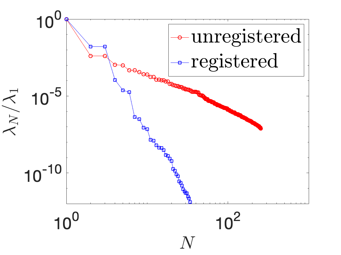
Figure 2 shows the behavior of ∥⋅∥2\|\cdot\|_{2}-POD eigenvalues associated with {𝐚μihf}i=1ntrain\{\mathbf{a}_{\mu^{i}}^{\rm hf}\}_{i=1}^{n_{\rm train}}, and the L2L^{2}-POD eigenvalues associated with {𝐊μi⋆}i=1ntrain\{\mathbf{K}_{\mu^{i}}^{\star}\}_{i=1}^{n_{\rm train}}. We remark that the decay of the POD eigenvalues cannot be directly related to the behavior of the Kolmogorov NN-width; nevertheless, POD eigenvalues provide an heuristic measure of the linear complexity of parametric manifolds and are thus shown in this paper to investigate performance of the registration algorithm.

Refer to caption
(a)

Refer to caption
(b)
Figure 2: reaction-diffusion problem with boundary layer. Behavior of POD eigenvalues. (a): ∥⋅∥2\|\cdot\|_{2}-POD for {𝐚μihf}i=1ntrain\{\mathbf{a}_{\mu^{i}}^{\rm hf}\}_{i=1}^{n_{\rm train}}. (b) L2L^{2}-POD for {𝐊μi⋆}i=1ntrain\{\mathbf{K}_{\mu^{i}}^{\star}\}_{i=1}^{n_{\rm train}}.

Results

Figure 3(a) shows the behavior of the solution field zμz_{\mu} for μ=20\mu=20; as anticipated above, the solution exhibits a boundary layer close to ΓD\Gamma_{\rm D}. In Figure 3(b) and (c), we show slices of the solution field t↦zμ​(t,t)t\mapsto z_{\mu}(t,t), t↦zμ​(t,0.5)t\mapsto z_{\mu}(t,0.5), for three parameter values along the straight lines depicted in Figure 3(a): as expected, the size of the boundary layer strongly depends on the value of μ\mu. In Figure 4, we reproduce the results of Figure 3 for the mapped field: we observe that the mapping procedure significantly reduces the sensitivity of the solution to the value of μ\mu.

Refer to caption
(a) zμz_{\mu}, μ=20\mu=20

Refer to caption
(b)

Refer to caption
(c)
Figure 3: reaction-diffusion problem with boundary layer. (a): behavior of zμ=20z_{\mu=20}. (b) and (c): behavior of zμ​(𝐱=(t,t))z_{\mu}(\mathbf{x}=(t,t)) and zμ​(𝐱=(t,0.5))z_{\mu}(\mathbf{x}=(t,0.5)) for three values of μ∈𝒫\mu\in\mathcal{P}, t∈[0,1]t\in[0,1].
Refer to caption
(a) z~μ\tilde{z}_{\mu}, μ=20\mu=20

Refer to caption
(b)

Refer to caption
(c)
Figure 4: reaction-diffusion problem with boundary layer. (a): behavior of z~μ=20\tilde{z}_{\mu=20}. (b) and (c): behavior of z~μ​(𝐗=(t,t))\tilde{z}_{\mu}(\mathbf{X}=(t,t)) and z~μ​(𝐗=(t,0.5))\tilde{z}_{\mu}(\mathbf{X}=(t,0.5)) for three values of μ∈𝒫\mu\in\mathcal{P}, t∈[0,1]t\in[0,1].

Figure 5(a) shows the behavior of the relative H1H^{1} projection error associated with the POD space in the physical (unregistered) and mapped (registered) configurations,

Eproj=maxμ∈{μj}j=1ntest⁡‖zμ−Π𝒵N​zμ‖H1​(Ω)‖zμ‖H1​(Ω),E~proj=maxμ∈{μi}i=1ntest⁡‖z~μ−Π𝒵N~​z~μ‖H1​(Ω)‖z~μ‖H1​(Ω),E_{\rm proj}=\max_{\mu\in\{\mu^{j}\}_{j=1}^{n_{\rm test}}}\frac{\|z_{\mu}-\Pi_{\mathcal{Z}_{N}}z_{\mu}\|_{H^{1}(\Omega)}}{\|z_{\mu}\|_{H^{1}(\Omega)}},\hskip 10.00002pt\widetilde{E}_{\rm proj}=\max_{\mu\in\{\mu^{i}\}_{i=1}^{n_{\rm test}}}\frac{\|\tilde{z}_{\mu}-\Pi_{\widetilde{\mathcal{Z}_{N}}}\tilde{z}_{\mu}\|_{H^{1}(\Omega)}}{\|\tilde{z}_{\mu}\|_{H^{1}(\Omega)}}, (34)

where μ1,…,μntest​∼iid​Uniform​(𝒫)\mu^{1},\ldots,\mu^{n_{\rm test}}\overset{\rm iid}{\sim}{\rm Uniform}(\mathcal{P}) (ntest=200n_{\rm test}=200) and the space {𝒵N}N\{\mathcal{Z}_{N}\}_{N} (resp., {𝒵~N}N\{\widetilde{\mathcal{Z}}_{N}\}_{N}) is built applying H1H^{1}-POD to the snapshot sets {zμi}i=1ntest\{z_{\mu^{i}}\}_{i=1}^{n_{\rm test}} (resp. {z~μi}i=1ntest\{\tilde{z}_{\mu^{i}}\}_{i=1}^{n_{\rm test}}). On the other hand, Figure 2(b) shows the H1H^{1}-POD eigenvalues associated with {zμi}i=1ntest\{z_{\mu^{i}}\}_{i=1}^{n_{\rm test}} (unregistered) and {z~μi}i=1ntest\{\tilde{z}_{\mu^{i}}\}_{i=1}^{n_{\rm test}} (registered). Note that E~proj≤Eproj\widetilde{E}_{\rm proj}\leq{E}_{\rm proj} for N≤6N\leq 6, while E~proj>Eproj\widetilde{E}_{\rm proj}>{E}_{\rm proj} for N>6N>6; similar behavior can be observed for the POD eigenvalues: to reduce the sensitivity of the solution to the value of μ\mu, the mapping process introduces some small-amplitude smaller spatial scale distortions, which then ultimately control the convergence. Nevertheless, we do emphasize that for N=1N=1 the relative error satisfies E~proj≲10−4\widetilde{E}_{\rm proj}\lesssim 10^{-4} and is thus comparable with the accuracy of the underlying truth discretization: as a result, the “complexity overhead” due to mapping-induced distortions has little practical importance for this model problem.

Refer to caption
(a)

Refer to caption
(b)
Figure 5: reaction-diffusion problem with boundary layer. (a): behavior of Eproj,E~projE_{\rm proj},\widetilde{E}_{\rm proj} (34) with NN. (b): behavior of the H1H^{1}-POD eigenvalues associated with {zμi}i=1ntest\{z_{\mu^{i}}\}_{i=1}^{n_{\rm test}} (unregistered) and {z~μi}i=1ntest\{\tilde{z}_{\mu^{i}}\}_{i=1}^{n_{\rm test}} (registered).

In Figure 6, we investigate the impact on performance of the choice of ξ\xi in (17). More in detail, we show the behavior of the proximity measure 𝔣​(𝐚hf​(μ),μ,μ¯)\mathfrak{f}(\mathbf{a}_{\rm hf}(\mu),\mu,\bar{\mu}) and of the mapping seminorm |𝚿𝐚hf​(μ)hf|H2​(Ω)|\boldsymbol{\Psi}_{\mathbf{a}_{\rm hf}(\mu)}^{\rm hf}|_{H^{2}(\Omega)} with respect to ξ\xi for three values of μ\mu in 𝒫\mathcal{P}, where 𝐚hf​(μ)\mathbf{a}_{\rm hf}(\mu) denotes the solution to (17) for a given μ∈𝒫\mu\in\mathcal{P}. Interestingly, the performance is nearly independent of ξ\xi for ξ≲10−8\xi\lesssim 10^{-8}, for all three choices of μ\mu.

Refer to caption
(a)

Refer to caption
(b)
Figure 6: reaction-diffusion problem with boundary layer. Sensitivity analysis with respect to ξ\xi in (17) for three values of μ∈𝒫\mu\in\mathcal{P}. (a): behavior of the optimal proximity measure 𝔣​(𝐚hf​(μ),μ,μ¯)\mathfrak{f}(\mathbf{a}_{\rm hf}(\mu),\mu,\bar{\mu}) with ξ\xi. (b): behavior of the mapping H2H^{2} seminorm with ξ\xi.

In Figure 7, we show the behavior of the proximity measure 𝔣​(𝐚hf​(μ),μ,μ¯)\mathfrak{f}(\mathbf{a}_{\rm hf}(\mu),\mu,\bar{\mu}) and of the mapping seminorm |𝚿𝐚hf​(μ)hf|H2​(Ω)|\boldsymbol{\Psi}_{\mathbf{a}_{\rm hf}(\mu)}^{\rm hf}|_{H^{2}(\Omega)} with respect to μ\mu, for two choices of the reference parameter, μ¯=μmin​μmax\bar{\mu}=\sqrt{\mu_{\rm min}\mu_{\rm max}} and μ¯=μmin+μmax2\bar{\mu}=\frac{\mu_{\rm min}+\mu_{\rm max}}{2}. For the second choice, we chose ϵ=0.05\epsilon=0.05. We observe that the first choice leads to superior performance in terms of accuracy and also reduces the maximum (over 𝒫\mathcal{P}) magnitude of the mapping seminorm: similarly to [35], we empirically observe that the choice of the reference field (template) u¯\bar{u} has a significant impact on performance.

Refer to caption
(a)

Refer to caption
(b)
Figure 7: reaction-diffusion problem with boundary layer. Sensitivity analysis with respect to the reference field u¯=uμ¯\bar{u}=u_{\bar{\mu}}. (a): behavior of the optimal proximity measure 𝔣​(𝐚hf​(μ),μ,μ¯)\mathfrak{f}(\mathbf{a}_{\rm hf}(\mu),\mu,\bar{\mu}) with μ\mu, for two choices of μ¯\bar{\mu}. (b): behavior of the mapping H2H^{2} seminorm with μ\mu, for two choices of μ¯\bar{\mu}.

3.4.2 Approximation of advection-dominated problems

Problem statement

We consider the advection-reaction problem:

{∇⋅(𝐜μ​zμ)+σμ​zμ=fμin​Ω=(0,1)2zμ=zD,μon​Γin,μ:={𝐱∈∂Ω:𝐜μ⋅𝐧<0}\left\{\begin{array}[]{ll}\nabla\cdot(\mathbf{c}_{\mu}z_{\mu})\,+\,\sigma_{\mu}z_{\mu}=f_{\mu}&{\rm in}\,\Omega=(0,1)^{2}\\ z_{\mu}=z_{\rm D,\mu}&{\rm on}\,\Gamma_{\rm in,\mu}:=\{\mathbf{x}\in\partial\Omega:\,\mathbf{c}_{\mu}\cdot\mathbf{n}<0\}\\ \end{array}\right. (35a)
where 𝐧\mathbf{n} denotes the outward normal to ∂Ω\partial\Omega, and
𝐜μ=[cos⁡(μ1)sin⁡(μ1)],σμ=1+μ2ex1+x2,fμ=1+x1x2,zD,μ=4​arctan⁡(μ3​(x2−12))​(x2−x22)μ=[μ1,μ2,μ3]∈𝒫:=[−π10,π10]×[0.3,0.7]×[60,100].\begin{array}[]{l}\displaystyle{\mathbf{c}_{\mu}=\left[\begin{array}[]{c}\cos(\mu_{1})\\ \sin(\mu_{1})\\ \end{array}\right],\quad\sigma_{\mu}=1+\mu_{2}e^{x_{1}+x_{2}},\quad f_{\mu}=1+x_{1}x_{2},}\\[8.53581pt] \displaystyle{z_{\rm D,\mu}=4\arctan\left(\mu_{3}\left(x_{2}-\frac{1}{2}\right)\right)\,\left(x_{2}-x_{2}^{2}\right)}\\[8.53581pt] \displaystyle{\mu=[\mu_{1},\mu_{2},\mu_{3}]\in\mathcal{P}:=\left[-\frac{\pi}{10},\frac{\pi}{10}\right]\times\left[0.3,0.7\right]\times\left[60,100\right].}\end{array} (35b)

Problem (35) is a parametric hyperbolic advection-reaction problem; since σμ+12∇⋅𝐜μ≥1>0\sigma_{\mu}+\frac{1}{2}\nabla\cdot\mathbf{c}_{\mu}\geq 1>0 for all 𝐱∈Ω\mathbf{x}\in\Omega, μ∈𝒫\mu\in\mathcal{P}, there exists a unique solution zμz_{\mu} to (35) for all μ∈𝒫\mu\in\mathcal{P}. We refer to [8, 15] for a mathematical analysis of the problem, and for the derivation of the infinite-dimensional variational form. We here resort to a DG P3 discretization on a structured triangular mesh with Nhf=23120N_{\rm hf}=23120 degrees of freedom to approximate (35); we denote by 𝒳\mathcal{X} the broken DG space equipped with the inner product (w,v):=∑k=1nel∫Dkw​v​𝑑x,(w,v):=\sum_{k=1}^{n_{\rm el}}\,\int_{\texttt{D}^{k}}\,w\,v\,dx, and the induced norm ∥⋅∥=(⋅,⋅)\|\cdot\|=\sqrt{(\cdot,\cdot)}. Note that changes in μ1\mu_{1} lead to changes in the large-gradient region associated with the solution zμz_{\mu} (cf. Figures (8)(a) and (b)), and are thus critical for linear approximation methods.

Exploiting the reasoning in section 3.3, we can derive the variational formulation for the mapped field z~μ\tilde{z}_{\mu}. We provide the explicit expressions of the terms in (27) in section C. Here, we remark that the size of the expansions in (29) are chosen based on the criterion in (5), with tolerance t​o​leim=5⋅10−7{tol}_{\rm eim}=5\cdot 10^{-7}.

Construction of the mapping

We set μ¯\bar{\mu} equal to the centroid of 𝒫\mathcal{P}, and we consider the proximity measure 𝔣\mathfrak{f} in (17b) with uμ=zμu_{\mu}=z_{\mu}. We further consider ξ=10−3\xi=10^{-3}, and we consider a polynomial expansion with M¯=6\overline{M}=6 in (11) (Mhf=72M_{\rm hf}=72). To build the regressor 𝐚^:𝒫→ℝM\widehat{\mathbf{a}}:\mathcal{P}\to\mathbb{R}^{M}, we consider ntrain=250n_{\rm train}=250 uniformly-sampled parameters in 𝒫\mathcal{P}, and we set t​o​lpod=10−4tol_{\rm pod}=10^{-4} in (5): for this choice of the parameters, the registration procedure returns an affine expansion with M=12M=12 terms.

As opposed to the previous problem, we do not expect that the mapping procedure will lead to a nearly one-dimensional mapped manifold; nevertheless, we do expect that the mapping procedure will reduce the sensitivity of the solution to parametric changes, particularly in μ1\mu_{1} — which regulates the position of the high-gradient region in Ω\Omega. For this reason, we here consider a larger value of the regularization parameter ξ\xi compared to the previous two examples: larger values of ξ\xi lead to smoother mappings and thus reduce the risk of overfitting and facilitate hyper-reduction. We further consider a lower value of MhfM_{\rm hf} (Mhf=72M_{\rm hf}=72 as opposed to Mhf=128M_{\rm hf}=128) compared to the previous example: in our numerical experience, the algorithm is insensitive to the choice of MhfM_{\rm hf}, for Mhf≥72M_{\rm hf}\geq 72.

Results

Figure 8 shows the solution to (35) for three values of the parameters μ1=[−π/10,0.3,60]\mu^{1}=[-\pi/10,0.3,60], μ2=[π/10,0.7,100]\mu^{2}=[\pi/10,0.7,100] and the centroid μ¯=[0,0.55,80]\bar{\mu}=[0,0.55,80]; on the other hand, Figure 9 shows the solution to the mapped problem z~μ=zμ∘𝚽μ\tilde{z}_{\mu}=z_{\mu}\circ\boldsymbol{\Phi}_{\mu} for the same three values of the parameter. As stated above, changes in μ1\mu_{1} lead to changes in the large-gradient region which corresponds to the propagation of the inflow boundary condition in the interior of Ω\Omega: the mapping 𝚽μ\boldsymbol{\Phi}_{\mu} significantly reduces the sensitivity of the solution to changes in the angle μ1\mu_{1}.

Refer to caption
(a) zμ1z_{\mu^{1}}

Refer to caption
(b) zμ2z_{\mu^{2}}

Refer to caption
(c) zμ¯z_{\bar{\mu}}
Figure 8: advection-reaction problem. Solution to (35) fo three parameter values.
Refer to caption
(a) z~μ1\tilde{z}_{\mu^{1}}

Refer to caption
(b) z~μ2\tilde{z}_{\mu^{2}}

Refer to caption
(c) zμ¯z_{\bar{\mu}}
Figure 9: advection-reaction problem. Solution to (35) fo three parameter values in the mapped configuration.

Figure 10(a) shows the behavior of the average relative L2L^{2} error

Eavg:=1ntest​∑i=1ntest‖zμi−z^μi‖L2​(Ω)‖zμi‖L2​(Ω),E_{\rm avg}:=\frac{1}{n_{\rm test}}\,\sum_{i=1}^{n_{\rm test}}\;\frac{\|z_{\mu^{i}}-\widehat{z}_{\mu^{i}}\|_{L^{2}(\Omega)}}{\|z_{\mu^{i}}\|_{L^{2}(\Omega)}},

for the L2L^{2}-POD-Galerkin ROM associated with the unregistered configuration, and for the L2L^{2}-POD-Galerkin ROM associated with the registered configuration. Here, μ1,…\mu^{1},\ldots, μntest\mu^{n_{\rm test}} ∼iid​Uniform​(𝒫)\overset{\rm iid}{\sim}{\rm Uniform}(\mathcal{P}), ntest=20n_{\rm test}=20. In order to use the same metric for both registered and unregistered ROMs, for the registered case we compute the error as

‖zμ−z^μ∘𝚽μ−1‖L2​(Ω)=∫Ω𝔍μ​(z~μ−z^μ)2​𝑑X.\|z_{\mu}-\widehat{z}_{\mu}\circ\boldsymbol{\Phi}_{\mu}^{-1}\|_{L^{2}(\Omega)}=\sqrt{\int_{\Omega}\,\mathfrak{J}_{\mu}\,\left(\widetilde{z}_{\mu}-\widehat{z}_{\mu}\right)^{2}\,dX}.

Figure 10(b) shows the L2​(Ω)L^{2}(\Omega)-POD eigenvalues associated with {zμi}i=1ntrain\{z_{\mu^{i}}\}_{i=1}^{n_{\rm train}} (unregistered) and {z~μi}i=1ntrain\{\tilde{z}_{\mu^{i}}\}_{i=1}^{n_{\rm train}} (registered).

Refer to caption
(a)

Refer to caption
(b)
Figure 10: advection-reaction problem. (a): behavior of EavgE_{\rm avg} with NN for the registered and unregistered POD-Galerkin ROMs. (b): behavior of L2​(Ω)L^{2}(\Omega)-POD eigenvalues associated with {zμi}i=1ntrain\{z_{\mu^{i}}\}_{i=1}^{n_{\rm train}} (unregistered) and {z~μi}i=1ntrain\{\tilde{z}_{\mu^{i}}\}_{i=1}^{n_{\rm train}} (registered).

We observe that the decay rates of EavgE_{\rm avg} and of the POD eigenvalues are nearly the same for both registered and unregistered configurations; however, the multiplicative constant is significantly different: Eavgreg.≈14​Eavgunreg.E_{\rm avg}^{\rm reg.}\approx\frac{1}{4}E_{\rm avg}^{\rm unreg.} for all values of NN considered, while (λNλ1)reg.≈1100​(λNλ1)unreg.\left(\frac{\lambda_{N}}{\lambda_{1}}\right)^{\rm reg.}\approx\frac{1}{100}\left(\frac{\lambda_{N}}{\lambda_{1}}\right)^{\rm unreg.} for N≥2N\geq 2. As a result, for any given NN, the nonlinear mapping procedure leads to a significant improvement. This empirical observation suggests a multiplicative effect between NN and MM approximations and is thus in good agreement with the estimate of the Kolmogorov N−MN-M width in (25). On the other hand, we remark that the mapping procedure leads to a significant increase in the number of EIM modes in (29). More in detail, for the registered case, we have

Qa,el=19,Qa,ed=26,Qf,el=15,Qf,ed=6;Q_{\rm a,el}=19,\hskip 10.00002ptQ_{\rm a,ed}=26,\hskip 10.00002ptQ_{\rm f,el}=15,\hskip 10.00002ptQ_{\rm f,ed}=6;

for the unregistered case, we have

Qa,el=4,Qa,ed=3,Qf,el=1,Qf,ed=2.Q_{\rm a,el}=4,\hskip 10.00002ptQ_{\rm a,ed}=3,\hskip 10.00002ptQ_{\rm f,el}=1,\hskip 10.00002ptQ_{\rm f,ed}=2.

Therefore, for any given NN, the registered ROM is more expensive in terms of memory than the unregistered ROM. This behavior of EIM can be explained by observing that most coefficients in (35) are parametrically affine in the unregistered configuration.

In Figure 11, we investigate the effect of the choice of ξ\xi in (17). Figures 11(a) and (b) show the behavior of the proximity measure 𝔣​(𝐚hf​(μ),μ,μ¯)\mathfrak{f}(\mathbf{a}_{\rm hf}(\mu),\mu,\bar{\mu}) and of the mapping seminorm |𝚿𝐚hf​(μ)hf|H2​(Ω)|\boldsymbol{\Psi}_{\mathbf{a}_{\rm hf}(\mu)}^{\rm hf}|_{H^{2}(\Omega)} with respect to ξ\xi for three values of μ\mu in 𝒫\mathcal{P}, where 𝐚hf​(μ)\mathbf{a}_{\rm hf}(\mu) denotes the solution to (17) for a given μ∈𝒫\mu\in\mathcal{P}. Figure 11(c) shows the decay of the mapping ∥⋅∥2\|\cdot\|_{2}-POD eigenvalues associated with {𝐚μihf}i=1ntrain\{\mathbf{a}_{\mu^{i}}^{\rm hf}\}_{i=1}^{n_{\rm train}} for two choices of ξ\xi. Similarly to the previous test case, both addends of the objective function converge to finite values for ξ→0+\xi\to 0^{+}; however, their numerical values and the threshold below which curves exhibit a plateau differ significantly between the two test cases. Furthermore, we observe that reducing ξ\xi leads to an increase of the complexity of the mapping manifold and ultimately increases the complexity of the generalization (cf. section 3.1.4) step.

Refer to caption
(a)

Refer to caption
(b)

Refer to caption
(c)
Figure 11: advection-reaction problem. Sensitivity analysis with respect to ξ\xi in (17) for three values of μ∈𝒫\mu\in\mathcal{P}. (a): behavior of the optimal proximity measure 𝔣​(𝐚hf​(μ),μ,μ¯)\mathfrak{f}(\mathbf{a}_{\rm hf}(\mu),\mu,\bar{\mu}) with ξ\xi. (b): behavior of the mapping H2H^{2} seminorm with ξ\xi. (c): decay of the ∥⋅∥2\|\cdot\|_{2}-POD eigenvalues associated with {𝐚μihf}i=1ntrain\{\mathbf{a}_{\mu^{i}}^{\rm hf}\}_{i=1}^{n_{\rm train}} for two choices of ξ\xi.

4 Geometry reduction

In this section, we discuss how to adapt the registration procedure introduced in section 3 to geometry reduction. In this paper, we shall assume that the reference domain Ω\Omega and the parameterized displacement field 𝐝μ:∂Ω→ℝd\mathbf{d}_{\mu}:\partial\Omega\to\mathbb{R}^{d} are given for all μ∈𝒫\mu\in\mathcal{P}: given 𝐗∈∂Ω\mathbf{X}\in\partial\Omega, we can thus compute the corresponding material point in the physical configuration as 𝐱μ=𝐗+𝐝μ​(𝐗)\mathbf{x}^{\mu}=\mathbf{X}+\mathbf{d}_{\mu}(\mathbf{X}). As discussed in the introduction, we remark that the boundary displacement — or equivalently a parameterization of the boundary ∂Ωμ\partial\Omega_{\mu} — might not be available for various classes of problems, including biological systems.

In view of the discussion, we further introduce the rectangle Ωbox=(a,b)×(c,d)\Omega_{\rm box}=(a,b)\times(c,d) such that Ω,Ωμ⊂Ωbox\Omega,\Omega_{\mu}\subset\Omega_{\rm box} for all μ∈𝒫\mu\in\mathcal{P}. Then, we introduce the parameterized function 𝚿hf\boldsymbol{\Psi}^{\rm hf} in (7), and we define the bases {𝝋mhf}m=1Mhf\{\boldsymbol{\varphi}_{m}^{\rm hf}\}_{m=1}^{M_{\rm hf}} as in (11) — after having applied a suitable change of variables.

4.1 Registration procedure

We introduce (i) the reference points {𝐗i}i=1Nbnd\{\mathbf{X}_{i}\}_{i=1}^{N_{\rm bnd}} ⊂∂Ω\subset\partial\Omega, (ii) the corresponding displaced points {𝐱ik=𝐗i+𝐝μk(𝐗i)}i,k\{\mathbf{x}_{i}^{k}=\mathbf{X}_{i}+\mathbf{d}_{\mu^{k}}(\mathbf{X}_{i})\}_{i,k} for some parameters μ1,…,μntrain∈𝒫\mu^{1},\ldots,\mu^{n_{\rm train}}\in\mathcal{P}, and (iii) the parameterized function 𝚿hf\boldsymbol{\Psi}^{\rm hf} (7) - (11). Then, for k=1,…,ntraink=1,\ldots,n_{\rm train}, we choose 𝐚hfk=𝐚hf​(μk)\mathbf{a}_{\rm hf}^{k}=\mathbf{a}_{\rm hf}(\mu^{k}) as a solution to

min𝐚∈ℝMhf⁡𝔣k​(𝐚)+ξ​|𝚿𝐚hf|H2​(Ωbox)2,s.t.∫Ωboxexp⁡(ϵ−𝔍𝐚hf​(𝐗)Cexp)+exp⁡(𝔍𝐚hf​(𝐗)−1/ϵCexp)​𝑑X≤δ,\begin{array}[]{l}\displaystyle{\min_{\mathbf{a}\in\mathbb{R}^{M^{\rm hf}}}\,\mathfrak{f}^{k}\left(\mathbf{a}\right)\,+\,\xi\big|\boldsymbol{\Psi}_{\mathbf{a}}^{\rm hf}\big|_{H^{2}(\Omega_{\rm box})}^{2},}\\[8.53581pt] \displaystyle{{\rm s.t.}\;\int_{\Omega_{\rm box}}\,{\rm exp}\left(\frac{\epsilon-\mathfrak{J}_{\mathbf{a}}^{\rm hf}(\mathbf{X})}{C_{\rm exp}}\right)\,+\,{\rm exp}\left(\frac{\mathfrak{J}_{\mathbf{a}}^{\rm hf}(\mathbf{X})-1/\epsilon}{C_{\rm exp}}\right)\,dX\leq\delta,}\\ \end{array} (36a)
where the proximity measure 𝐟k​(𝐚)=𝔣⁡(𝐚,μk)\mathbf{f}^{k}(\mathbf{a})=\mathfrak{f}\left(\mathbf{a},\mu^{k}\right) is given by
𝔣⁡(𝐚,μ):=1Nbnd​∑i=1Nbnd‖𝚿𝐚hf​(𝐗i)−𝐱iμ‖22.\mathfrak{f}\left(\mathbf{a},\mu\right):=\;\frac{1}{N_{\rm bnd}}\,\sum_{i=1}^{N_{\rm bnd}}\,\big\|\boldsymbol{\Psi}_{\mathbf{a}}^{\rm hf}\left(\mathbf{X}_{i}\right)\,-\,\mathbf{x}_{i}^{\mu}\big\|_{2}^{2}. (36b)

Given the dataset {(μk,𝐚hfk)}k=1ntrain\{(\mu^{k},\mathbf{a}_{\rm hf}^{k})\}_{k=1}^{n_{\rm train}}, we proceed as in section 3.1.4 to generate the mapping 𝚽:Ω×𝒫→ℝd\boldsymbol{\Phi}:\Omega\times\mathcal{P}\to\mathbb{R}^{d}.

We observe that (36) differs from (17) due to the choice of the proximity measure. Here, 𝔣\mathfrak{f} is an approximation of the L2​(∂Ω)L^{2}(\partial\Omega) error over the boundary

𝔣⁡(𝐚,μ)≈𝔣∞​(𝐚,μ):=∫∂Ω‖𝚿𝐚hf​(𝐗)−𝐗−𝐝μ​(𝐗)‖22​𝑑X.\mathfrak{f}\left(\mathbf{a},\mu\right)\approx\mathfrak{f}^{\infty}\left(\mathbf{a},\mu\right):=\int_{\partial\Omega}\,\|\boldsymbol{\Psi}_{\mathbf{a}}^{\rm hf}\left(\mathbf{X}\right)\,-\,\mathbf{X}-\mathbf{d}_{\mu}(\mathbf{X})\,\|_{2}^{2}\,dX.

If 𝔣∞​(𝐚hf,μ)=0\mathfrak{f}^{\infty}(\mathbf{a}^{\rm hf},\mu)=0 for some admissible 𝐚hf∈ℝM\mathbf{a}^{\rm hf}\in\mathbb{R}^{M} and Ω\Omega satisfies the hypotheses of Proposition 2.1, recalling Proposition 2.4, we find that 𝚿𝐚hf\boldsymbol{\Psi}_{\mathbf{a}}^{\rm hf} is a bijection from Ω\Omega to Ωμ\Omega_{\mu}. We further remark that, if 𝚿𝐚hf\boldsymbol{\Psi}_{\mathbf{a}}^{\rm hf} is a bijection from Ωbox\Omega_{\rm box} into itself, it is injective in Ω\Omega.

Remark 4.1.

Implicit surfaces. If ∂Ωμ\partial\Omega_{\mu} is represented implicitly as ∂Ωμ={𝐱∈ℝd:Gμ​(𝐱)=0}\partial\Omega_{\mu}=\{\mathbf{x}\in\mathbb{R}^{d}:\;\mathit{G}_{\mu}(\mathbf{x})=0\} for Gμ:ℝd→ℝ\mathit{G}_{\mu}:\mathbb{R}^{d}\to\mathbb{R}, then we might consider the proximity measure:

𝔣⁡(𝐚,μ,μ¯)=1Nbnd​∑i=1Nbnd|Gμ​(𝚿𝐚hf​(𝐗i))|2\mathfrak{f}(\mathbf{a},\mu,\bar{\mu})\,=\,\frac{1}{N_{\rm bnd}}\,\sum_{i=1}^{N_{\rm bnd}}\,\big|\mathit{G}_{\mu}\left(\boldsymbol{\Psi}_{\mathbf{a}}^{\rm hf}(\mathbf{X}_{i})\right)\big|^{2}

where {𝐗i}i\{\mathbf{X}_{i}\}_{i} is the set of control points on ∂Ω\partial\Omega. We do not consider this choice in the numerical experiments.

4.2 Model problems

We present below the two model problems considered in the numerical experiments.

4.2.1 Diffusion problem with discontinuous coefficients

We consider the diffusion problem

−∇⋅(κμ∇zμ)= 1inΩbox,zμ|∂Ωbox=0,-\nabla\cdot\left(\kappa_{\mu}\nabla z_{\mu}\right)\,=\,1\;\;{\rm in}\;\Omega_{\rm box},\hskip 10.00002ptz_{\mu}\big|_{\partial\Omega_{\rm box}}=0, (37a)
where Ωbox=(0,1)2\Omega_{\rm box}=(0,1)^{2}, μ=[μ1,μ2]∈𝒫=[−0.05,0.05]2\mu=[\mu_{1},\mu_{2}]\in\mathcal{P}=[-0.05,0.05]^{2} and the conductivity coefficient is given by
κμ​(𝐱):= 0.1+ 0.9​ 1Ωμ​(𝐱),Ωμ:={𝐱∈Ω:‖𝐱−𝐱¯μ‖∞≤14},\kappa_{\mu}(\mathbf{x}):=\,0.1\,+\,0.9\,\mathbbm{1}_{\Omega_{\rm\mu}}(\mathbf{x}),\hskip 10.00002pt\Omega_{\rm\mu}:=\{\mathbf{x}\in\Omega:\,\|\mathbf{x}-\bar{\mathbf{x}}_{\mu}\|_{\infty}\leq\frac{1}{4}\}, (37b)
with 𝐱¯μ:=[1/2+μ1,1/2+μ2]\bar{\mathbf{x}}_{\mu}:=[1/2+\mu_{1},1/2+\mu_{2}]. The problem is a variant of the thermal block problem, which has been extensively considered in the reduced basis literature (see, e.g., [53, section 6.1.1]). We here approximate the solution to (37) through a continuous Galerkin P3 FE discretization with Nhf=21025N_{\rm hf}=21025 degrees of freedom.

Since κμ\kappa_{\mu} is piecewise constant with parameter-dependent jump discontinuities, pMOR techniques are not well-suited to directly tackle (37). It is thus necessary to introduce a mapping 𝚽:Ωbox×𝒫→Ωbox\boldsymbol{\Phi}:\Omega_{\rm box}\times\mathcal{P}\to\Omega_{\rm box} such that κμ∘Φμ:Ωbox→ℝ\kappa_{\mu}\circ\Phi_{\mu}:\Omega_{\rm box}\to\mathbb{R} is parameter-independent. From the geometry reduction viewpoint, given Ω:=Ωμ=0\Omega:=\Omega_{\rm\mu=0}, we seek 𝚽\boldsymbol{\Phi} such that (i) 𝚽μ​(Ωbox)=Ωbox\boldsymbol{\Phi}_{\mu}(\Omega_{\rm box})=\Omega_{\rm box} and (ii) 𝚽μ​(Ω)=Ωμ\boldsymbol{\Phi}_{\mu}(\Omega)=\Omega_{\mu} for all μ∈𝒫\mu\in\mathcal{P}. In view of the discussion, we introduce the mapped problem for a generic map 𝚽μ:Ωbox→Ωbox\boldsymbol{\Phi}_{\mu}:\Omega_{\rm box}\to\Omega_{\rm box}: find z~μ=zμ∘𝚽μ∈𝒳:=H01​(Ωbox)\tilde{z}_{\mu}=z_{\mu}\circ\boldsymbol{\Phi}_{\mu}\in\mathcal{X}:=H_{0}^{1}(\Omega_{\rm box}) such that

∫Ωbox𝐊μ⋆​∇^​z~μ⋅∇^​v​𝑑X=∫Ωbox𝔍μ​v​𝑑X,∀v∈𝒳,\int_{\Omega_{\rm box}}\,\mathbf{K}_{\mu}^{\star}\widehat{\nabla}\tilde{z}_{\mu}\cdot\widehat{\nabla}v\,dX\,=\,\int_{\Omega_{\rm box}}\,\mathfrak{J}_{\mu}\,vdX,\;\;\forall\,v\in\mathcal{X}, (38a)
with
𝐊μ⋆:=𝔍μ​(κμ∘𝚽μ)​(∇^​𝚽μ)−1​(∇^​𝚽μ)−T,𝔍μ:=det⁡(∇^​𝚽μ).\mathbf{K}_{\mu}^{\star}:=\mathfrak{J}_{\mu}\,\left(\kappa_{\mu}\,\circ\boldsymbol{\Phi}_{\mu}\right)\,\left(\widehat{\nabla}\boldsymbol{\Phi}_{\mu}\right)^{-1}\,\left(\widehat{\nabla}\boldsymbol{\Phi}_{\mu}\right)^{-T},\hskip 10.00002pt\mathfrak{J}_{\mu}:={\rm det}\left(\widehat{\nabla}\boldsymbol{\Phi}_{\mu}\right). (38b)

Note that (37) is a special case of the general advection-diffusion-reaction problem considered in section 3.3.

Automatic piecewise-affine maps

Since the deformation of Ωμ\Omega_{\mu} is rigid, we might explicitly build a piecewise linear map 𝚽\boldsymbol{\Phi}. First, we identify a set of control points — the black dots in Figure 12(a) — and we use them to build a coarse partition of Ωbox\Omega_{\rm box} — shown in Figure 12(a) as well. Then, we define a mapping 𝚽=𝚽aff\boldsymbol{\Phi}=\boldsymbol{\Phi}^{\rm aff} such that (i) Φμaff​(Ω)=Ωμ\Phi_{\mu}^{\rm aff}({\Omega})=\Omega_{\mu} for all μ∈𝒫\mu\in\mathcal{P}, and (ii) 𝚽μaff\boldsymbol{\Phi}_{\mu}^{\rm aff} is piecewise linear in 𝐗\mathbf{X} in all elements of the partition. Then, we define the mapped problem (38) with 𝚽μ=𝚽μaff\boldsymbol{\Phi}_{\mu}=\boldsymbol{\Phi}_{\mu}^{\rm aff}.

Note that, for this choice of the mapping, 𝐊μ⋆\mathbf{K}_{\mu}^{\star} and 𝔍μ\mathfrak{J}_{\mu} in (38b) are piecewise-constant in each element of the partition: this implies that (38) is parametrically-affine — that is, 𝐊μ⋆\mathbf{K}_{\mu}^{\star} and 𝔍μ\mathfrak{J}_{\mu} are linear combinations of parameter-dependent coefficients and parameter-independent spatial fields. Therefore, the solution z~μ\widetilde{z}_{\mu} can be efficiently approximated using standard pMOR (e.g., Reduced Basis) techniques.

Given the user-defined control points, Rozza el al. have developed in [53] an automatic procedure to generate the partition of Ωbox\Omega_{\rm box} and to determine an economic piecewise-constant approximation of the form in (38). The latter relies on symbolic manipulation techniques to identify redundant terms in the affine expansions. Furthermore, for the approach to be effective, we should consider FE triangulations that are conforming to the coarse-grained partition in Figure 12(a). Finally, the choice of the control points, which is trivial in this case, might not be straightforward for more challenging problems. In conclusion, even if the approach works remarkably well in many situations, practical implementation of the procedure in [53] is rather involved and highly problem-dependent.

4.2.2 Laplace’s equation in parameterized domains

Given the parameter domain 𝒫=[0.1,0.4]2×[0,π/4]\mathcal{P}=[0.1,0.4]^{2}\times[0,\pi/4], we first introduce the parametric closed curve t∈[0,2​π)↦𝜸in,μ​(t)∈ℝ2t\in[0,2\pi)\mapsto\boldsymbol{\gamma}_{\rm in,\mu}(t)\in\mathbb{R}^{2} such that

𝜸in,μ​(t)=[cos⁡(t)​(1+μ1​(cos⁡(t+μ3))2+ 2⋅10−3​((2​π−t)​t)2)sin⁡(t)​(1+μ2​(sin⁡(t+μ3))2+ 2⋅10−3​((2​π−t)​t)2)]\boldsymbol{\gamma}_{\rm in,\mu}(t)=\left[\begin{array}[]{l}\displaystyle{\cos(t)\left(1+\mu_{1}\,\left(\cos(t+\mu_{3})\right)^{2}\,+\,2\cdot 10^{-3}\left((2\pi-t)\,t\right)^{2}\right)}\\[8.53581pt] \displaystyle{\sin(t)\left(1+\mu_{2}\,\left(\sin(t+\mu_{3})\right)^{2}\,+\,2\cdot 10^{-3}\left((2\pi-t)\,t\right)^{2}\right)}\\ \end{array}\right] (39a)
and we denote by Ωin,μ\Omega_{\rm in,\mu} the bounded domain such that ∂Ωin,μ=𝜸μ​([0,2​π])\partial\Omega_{\rm in,\mu}=\boldsymbol{\gamma}_{\mu}([0,2\pi]) for all μ∈𝒫\mu\in\mathcal{P}. We further define Ωbox=(−2,2)2\Omega_{\rm box}=(-2,2)^{2}: note that Ωin,μ⋐Ωbox\Omega_{\rm in,\mu}\Subset\Omega_{\rm box} for all μ∈𝒫\mu\in\mathcal{P}. Then, we introduce the Laplace’s problem:
−Δ​zμ= 0in​Ωμ,zμ|∂Ωin,μ= 1,zμ|∂Ωbox= 0,-\Delta\,z_{\mu}\,=\,0\hskip 10.00002pt{\rm in}\,\Omega_{\mu},\hskip 20.00003ptz_{\mu}\big|_{\partial\Omega_{\rm in,\mu}}\,=\,1,\hskip 10.00002ptz_{\mu}\big|_{\partial\Omega_{\rm box}}\,=\,0, (39b)
where Ωμ:=Ωbox∖Ωin,μ\Omega_{\mu}:=\Omega_{\rm box}\setminus\Omega_{\rm in,\mu} is depicted in Figures 12(c) and 12(d) for two values of μ∈𝒫\mu\in\mathcal{P}.

We introduce the reference domain Ω=Ωbox∖Ωin\Omega=\Omega_{\rm box}\setminus\Omega_{\rm in}, with Ωin=ℬ1​(𝟎)\Omega_{\rm in}=\mathcal{B}_{1}(\mathbf{0}): note that Ω\Omega is diffeomorphic to Ωμ\Omega_{\mu} for all μ∈𝒫\mu\in\mathcal{P}. Then, given the bijection 𝚽μ:Ω→Ωμ\boldsymbol{\Phi}_{\mu}:\Omega\to\Omega_{\mu}, and the lift RDR_{\rm D} such that

−Δ​RD= 0in​Ω,RD|∂Ωin= 1,RD|∂Ωbox= 0,-\Delta\,R_{\rm D}\,=\,0\hskip 10.00002pt{\rm in}\,\Omega,\hskip 20.00003ptR_{\rm D}\big|_{\partial\Omega_{\rm in}}\,=\,1,\hskip 10.00002ptR_{\rm D}\big|_{\partial\Omega_{\rm box}}\,=\,0, (40a)
we define the mapped problem for the lifted solution: find z~μ∈𝒳:=H01​(Ω)\tilde{z}_{\mu}\in\mathcal{X}:=H_{0}^{1}(\Omega) such that
∫Ω𝐊μ⋆​∇^​(z~μ+RD)⋅∇^​v​𝑑X= 0,∀v∈𝒳,\int_{\Omega}\,\mathbf{K}_{\mu}^{\star}\widehat{\nabla}\left(\tilde{z}_{\mu}+R_{\rm D}\right)\cdot\widehat{\nabla}v\,dX\,=\,0,\;\;\forall\,v\in\mathcal{X}, (40b)
with 𝐊μ⋆:=𝔍μ​(∇^​𝚽μ)−1​(∇^​𝚽μ)−T\mathbf{K}_{\mu}^{\star}:=\mathfrak{J}_{\mu}\,\left(\widehat{\nabla}\boldsymbol{\Phi}_{\mu}\right)^{-1}\,\left(\widehat{\nabla}\boldsymbol{\Phi}_{\mu}\right)^{-T}.
Ω{\Omega}Ωbox{\Omega}_{\rm box}
(a)

Refer to caption
(b)
Refer to caption
(c)

Refer to caption
(d)
Figure 12: geometry reduction. (a): affine geometry (section 4.2.1). Black dots denote the user-defined control points associated with the coarse triangulation. (b)-(d): non-affine geometry (section 4.2.2). (b): reference domain Ω\Omega; (c)-(d): domain Ωμ\Omega_{\mu} for two values of μ∈𝒫\mu\in\mathcal{P}.

4.2.3 Application of the registration procedure

We consider the parametric function 𝚿hf\boldsymbol{\Psi}^{\rm hf} (7) - (11): thanks to this choice, control points on ∂Ωbox\partial\Omega_{\rm box} are not necessary. Since, as in the examples of section 3, the conductivity matrix 𝐊μ⋆\mathbf{K}_{\mu}^{\star} and the Jacobian determinant 𝔍μ\mathfrak{J}_{\mu} are not expected to be affine, we resort to EIM,

𝐊μ⋆≈𝐊μeim:=∑q=1QaΘμq,κ​𝐊q,𝔍μ⋆≈𝔍μeim:=∑q=1QfΘμq,𝔧​𝔍q,\mathbf{K}_{\mu}^{\star}\approx\mathbf{K}_{\mu}^{\rm eim}:=\sum_{q=1}^{Q_{\rm a}}\,\Theta_{\mu}^{q,\kappa}\,\mathbf{K}_{q},\hskip 10.00002pt\mathfrak{J}_{\mu}^{\star}\approx\mathfrak{J}_{\mu}^{\rm eim}:=\sum_{q=1}^{Q_{\rm f}}\,\Theta_{\mu}^{q,\mathfrak{j}}\,\mathfrak{J}_{q}, (41)

to obtain a parametrically-affine surrogate model. As explained in section D, the basis functions are built using POD: the size of the expansions Qa,QfQ_{\rm a},Q_{\rm f} is chosen based on the criterion in (5).

Some comments are in order. Our approach leads to a non-affine formulation —and thus requires hyper-reduction to achieve online efficiency — for both problems; on the other hand, we observe that the approach exclusively relies on the parameterization of the boundary ∂Ωin,μ\partial\Omega_{\rm in,\mu} and can be applied for virtually any choice of the conductivity.

4.3 Numerical results

We present below results for the two model problems introduced in section 4.2. Since the focus of this section is geometry reduction, we do not discuss the construction of the ROM for the mapped problems (38) and (40).

4.3.1 Diffusion problem with discontinuous coefficients

We choose ξ=4⋅10−4\xi=4\cdot 10^{-4}, t​o​lPOD=10−5tol_{\rm POD}=10^{-5}, M¯=6\overline{M}=6 (Mhf=72M_{\rm hf}=72); furthermore, we consider the proximity measure (36b) where {𝐗i}i=1Nbnd\{\mathbf{X}_{i}\}_{i=1}^{N_{\rm bnd}} is an uniform grid of ∂Ωin\partial\Omega_{\rm in} with Nbnd=400N_{\rm bnd}=400 and {𝐱iμ=𝐗i+μ}i\{\mathbf{x}_{i}^{\mu}=\mathbf{X}_{i}\,+\,\mu\}_{i}; finally, we consider ntrain=162n_{\rm train}=16^{2} equispaced parameters in 𝒫\mathcal{P}. For this choice of the parameters, our procedure returns an affine expansion with M=6M=6 terms.

In Figure 13, we investigate the (linear) complexity of the parametric manifolds associated with (37). In Figure 13(a), we compute the L2​(Ωbox)L^{2}(\Omega_{\rm box})-POD eigenvalues associated with {κμk}k=1ntrain\{\kappa_{\mu^{k}}\}_{k=1}^{n_{\rm train}} (unregistered) and {κ~μk=κμk∘𝚽μk}k=1ntrain\{\widetilde{\kappa}_{\mu^{k}}=\kappa_{\mu^{k}}\circ\boldsymbol{\Phi}_{\mu^{k}}\}_{k=1}^{n_{\rm train}} (registered). We observe that λN=2≤10−15​λN=1\lambda_{N=2}\leq 10^{-15}\lambda_{N=1} for the registered case: the mapping 𝚽μ\boldsymbol{\Phi}_{\mu} is able to ‘‘fix” the position of the jump discontinuity in the reference configuration44 4 More precisely, if we denote by {𝐱qin}q\{\mathbf{x}_{q}^{\rm in}\}_{q} (resp. {𝐱qout}q\{\mathbf{x}_{q}^{\rm out}\}_{q}) the FE quadrature points in Ω\Omega (resp. Ωbox∖Ω\Omega_{\rm box}\setminus\Omega), we have that 𝚽μ​({𝐱qin}q)⊂Ωμ\boldsymbol{\Phi}_{\mu}(\{\mathbf{x}_{q}^{\rm in}\}_{q})\subset\Omega_{\mu} (resp. 𝚽μ​({𝐱qout}q)⊂Ωbox∖Ωμ\boldsymbol{\Phi}_{\mu}(\{\mathbf{x}_{q}^{\rm out}\}_{q})\subset\Omega_{\rm box}\setminus\Omega_{\mu}) for all μ∈𝒫\mu\in\mathcal{P}.. In Figure 13(b), we show the L2​(Ωbox)L^{2}(\Omega_{\rm box})-POD eigenvalues of {𝐊μk⋆}k=1ntrain\{\mathbf{K}_{\mu^{k}}^{\star}\}_{k=1}^{n_{\rm train}} and {𝔍μk}k=1ntrain\{\mathfrak{J}_{\mu^{k}}\}_{k=1}^{n_{\rm train}}. Finally, in Figure 13(c), we show the behavior of the H1​(Ωbox)H^{1}(\Omega_{\rm box})-POD eigenvalues of {zμk}k=1ntrain\{z_{\mu^{k}}\}_{k=1}^{n_{\rm train}} (unregistered) and {z~μk}k=1ntrain\{\widetilde{z}_{\mu^{k}}\}_{k=1}^{n_{\rm train}} (registered): even if the mapping is built based on the diffusivity coefficient, it is also effective in improving the linear reducibility of the solution manifold.
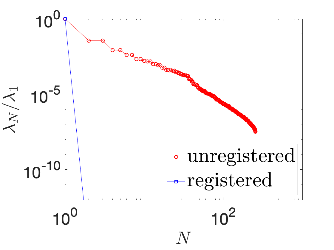
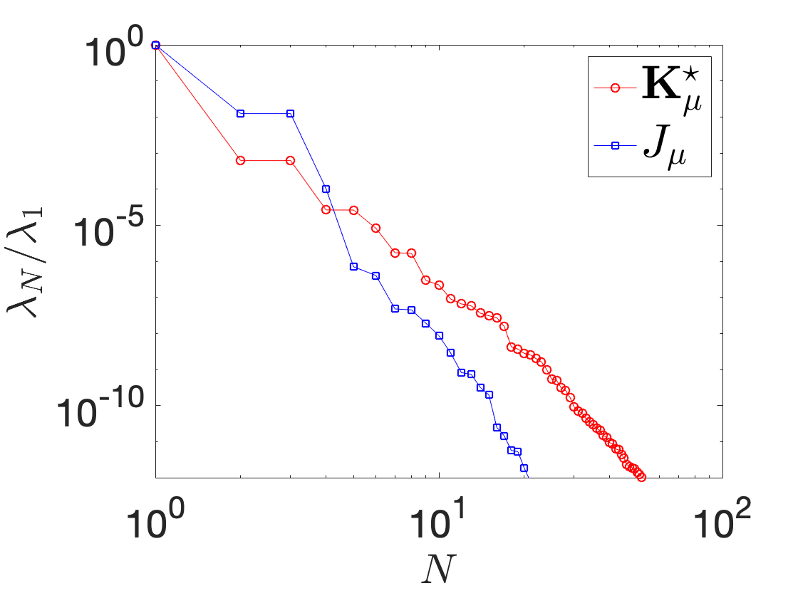
Refer to caption
(a)

Refer to caption
(b)

Refer to caption
(c)
Figure 13: diffusion problem with discontinuous coefficients. Behavior of POD eigenvalues associated with {κμk}k\{\kappa_{\mu^{k}}\}_{k} and {κ~μk}k\{\tilde{\kappa}_{\mu^{k}}\}_{k} (Fig. (a)), {𝐊μk⋆}k\{\mathbf{K}_{\mu^{k}}^{\star}\}_{k} and {𝔍μk}k\{\mathfrak{J}_{\mu^{k}}\}_{k} (Fig. (b)), and {zμk}k\{z_{\mu^{k}}\}_{k} and {z~μk}k\{\tilde{z}_{\mu^{k}}\}_{k} (Fig. (c)).

In Figure 14, we show the behavior of the mean relative error

Eavg:=1ntest​∑i=1ntest‖z~μi−z~μieim‖⋆‖z~μi‖⋆,μ1,…,μntest​∼iid​Uniform​(𝒫),E_{\rm avg}:=\frac{1}{n_{\rm test}}\,\sum_{i=1}^{n_{\rm test}}\,\frac{\|\tilde{z}_{\mu^{i}}-\tilde{z}_{\mu^{i}}^{\rm eim}\|_{\star}}{\|\tilde{z}_{\mu^{i}}\|_{\star}},\hskip 10.00002pt\mu^{1},\ldots,\mu^{n_{\rm test}}\overset{\rm iid}{\sim}{\rm Uniform}(\mathcal{P}), (42)

with respect to the tolerance t​o​leimtol_{\rm eim} associated with the choice of Qa,QfQ_{\rm a},Q_{\rm f} in (41), for ntest=20n_{\rm test}=20. Here, ∥⋅∥⋆\|\cdot\|_{\star} denotes either the L2​(Ω)L^{2}(\Omega) norm or the H1​(Ω)H^{1}(\Omega) norm:

‖w‖L2​(Ωbox)2=∫Ωbox|w|2​𝑑x,‖w‖H1​(Ωbox)2=∫Ωbox|w|2+‖∇w‖22​𝑑x.\|w\|_{L^{2}(\Omega_{\rm box})}^{2}=\int_{\Omega_{\rm box}}\,|w|^{2}\,dx,\hskip 10.00002pt\|w\|_{H^{1}(\Omega_{\rm box})}^{2}=\int_{\Omega_{\rm box}}\,|w|^{2}\,+\|\nabla w\|_{2}^{2}dx.

In Figure 14(b), we show the behavior of Qa,QfQ_{\rm a},Q_{\rm f} with respect to t​o​leimtol_{\rm eim}: we observe that the relative H1H^{1} and L2L^{2} errors are less than 10−310^{-3}, for Qa=19,Qf=9Q_{\rm a}=19,Q_{\rm f}=9. We remark that using piecewise-affine mappings (cf. section 4.2.1) we might obtain an exact affine form with Qa=13,Qf=3Q_{\rm a}=13,Q_{\rm f}=3. Once again, we remark that our approach is fully automatic.

Refer to caption
(a)

Refer to caption
(b)
Figure 14: diffusion problem with discontinuous coefficients. (a): behavior of EavgE_{\rm avg} (42) with t​o​leimtol_{\rm eim} (ntest=20n_{\rm test}=20). (b): behavior of Qa,QfQ_{\rm a},Q_{\rm f} in (41) with t​o​leimtol_{\rm eim}.

4.3.2 Laplace’s equation in parameterized domains

We choose ξ=10−2\xi=10^{-2}, t​o​lPOD=10−5tol_{\rm POD}=10^{-5}, Mhf=288M_{\rm hf}=288, and we define the proximity measure 𝔣\mathfrak{f} (36b) based on Nbnd=103N_{\rm bnd}=10^{3} points {𝐗i=𝜸ref(2πi/Nbnd)}i=1Nbnd\{\mathbf{X}_{i}=\boldsymbol{\gamma}^{\rm ref}(2\pi i/N_{\rm bnd})\}_{i=1}^{N_{\rm bnd}} with 𝜸ref​(t)=[cos⁡(t),sin⁡(t)]\boldsymbol{\gamma}^{\rm ref}(t)=[\cos(t),\sin(t)]. To generate the mapping, we consider uniform grids of 𝒫\mathcal{P} {μk}k=1ntrain\{\mu^{k}\}_{k=1}^{n_{\rm train}} with ntrain=43,63,83,103n_{\rm train}=4^{3},6^{3},8^{3},10^{3}.

In Figure 15, we show boxplots of the “in-sample” and “out-of-sample” errors given by

{Ekgeo,in:=maxi=1,…,Nbnd⁡‖𝚿𝐚hfkhf​(𝐗i)−𝐱iμk‖2k=1,…,ntrainEjgeo,out:=maxi=1,…,Nbndt⁡dist⁡(𝚽μ~j​(𝐗it),{𝐱i′,jt}i′=1Nbndt)j=1,…,ntest\left\{\begin{array}[]{ll}\displaystyle{E_{k}^{\rm geo,in}:=\max_{i=1,\ldots,N_{\rm bnd}}\,\|\boldsymbol{\Psi}_{\mathbf{a}_{\rm hf}^{k}}^{\rm hf}(\mathbf{X}_{i})-\mathbf{x}_{i}^{\mu^{k}}\|_{2}}&\displaystyle{k=1,\ldots,n_{\rm train}}\\[8.53581pt] \displaystyle{E_{j}^{\rm geo,out}:=\max_{i=1,\ldots,N_{\rm bnd}^{\rm t}}\,{\rm dist}\left(\boldsymbol{\Phi}_{\tilde{\mu}^{j}}(\mathbf{X}_{i}^{\rm t}),\,\{\mathbf{x}_{i^{\prime},j}^{\rm t}\}_{i^{\prime}=1}^{N_{\rm bnd}^{\rm t}}\right)}&\displaystyle{j=1,\ldots,n_{\rm test}}\\ \end{array}\right. (43)

where {𝐗it=𝜸ref(ti)}i\{\mathbf{X}_{i}^{\rm t}=\boldsymbol{\gamma}^{\rm ref}(t^{i})\}_{i} and {𝐱i,jt=𝜸μ~j(ti)}i\{\mathbf{x}_{i,j}^{\rm t}=\boldsymbol{\gamma}_{\tilde{\mu}^{j}}(t^{i})\}_{i}, with ti=2​π​iNbndtt^{i}=\frac{2\pi i}{N_{\rm bnd}^{\rm t}}, μ~1,…,μ~ntest​∼iid​Uniform​(𝒫)\tilde{\mu}^{1},\ldots,\tilde{\mu}^{n_{\rm test}}\overset{\rm iid}{\sim}{\rm Uniform}(\mathcal{P}), Nbndt=104N_{\rm bnd}^{\rm t}=10^{4}, ntest=50n_{\rm test}=50. In-sample error depends on the choice of the hyper- parameters in (17) and on the choice of the discretization parameter MhfM_{\rm hf}; on the other hand, out-of-sample error depends on the choice of t​o​lPODtol_{\rm POD} and on the number of training points. Interestingly, the value of MM is the same (and equal to 77) for all choices of ntrainn_{\rm train}.

Refer to caption
(a) ntrain=43n_{\rm train}=4^{3}

Refer to caption
(b) ntrain=63n_{\rm train}=6^{3}
Refer to caption
(c) ntrain=83n_{\rm train}=8^{3}

Refer to caption
(d) ntrain=103n_{\rm train}=10^{3}
Figure 15: Laplace’s equation in parameterized domain; performance of the registration procedure. Boxplots of in-sample and out-of-sample errors EgeoE_{\rm geo} for several training sizes.

Figure 16 replicates the results of Figure 14 for the second model problem. Here, we consider ntrain=103n_{\rm train}=10^{3}, ξ=10−2\xi=10^{-2}, Mhf=288M_{\rm hf}=288, t​o​lPOD=10−5tol_{\rm POD}=10^{-5}, and we compute EavgE_{\rm avg} (42) based on ntest=50n_{\rm test}=50 parameters. We find that the relative L2L^{2} and H1H^{1} errors are below 10−310^{-3} for QaQ_{\rm a} equal to 1717.

Refer to caption
(a)

Refer to caption
(b)
Figure 16: Laplace’s equation in parameterized domain; performance of the registration procedure. (a): behavior of EavgE_{\rm avg} (42) with t​o​leimtol_{\rm eim} (ntest=50n_{\rm test}=50). (b): behavior of QaQ_{\rm a} in (41) with t​o​leimtol_{\rm eim}.

In the supplementary material (cf. section E), we further provide a numerical comparison of our approach with a representative mapping procedure for a given value of μ\mu.

5 Summary and discussion

In this work, we proposed a general (i.e., independent of the underlying PDE model) registration procedure, and we applied it to data compression and geometry reduction: in data compression, our registration procedure is used in combination with a linear compression method to devise a Lagrangian nonlinear compression method; in geometry reduction, our registration procedure is used to build a parametric mapping from a reference domain to a family of parameterized domains {Ωμ}μ∈𝒫\{\Omega_{\mu}\}_{\mu\in\mathcal{P}}. Several numerical results empirically motivate our proposal. Although the examples considered are rather academic, we believe that our results demonstrate the applicability ìof our approach to a broad class of relevant problems in science and engineering.

In the future, we wish to extend the approach in several directions. First, in this work, we chose the reference field u¯\bar{u} (cf. section 3) and the reference domain Ω\Omega (cf. section 4) that enters in the optimization statement a priori; in the future, we wish to develop automatic procedures to adaptively choose u¯\bar{u} and Ω\Omega. Second, in order to tackle problems with more complex parametric behaviors, we wish to develop partitioning techniques that leverage the use of multiple references, and we also wish to couple the approach with domain decomposition techniques. Third, as discussed in section 3.1, a major limitation of our approach is the need for several offline simulations to build the mapping 𝚽\boldsymbol{\Phi}. To address this issue, we wish to exploit recent advances in multi-fidelity approaches to reduce the offline computational burden. Alternatively, we wish to assess performance of projection methods to simultaneously learn mapping and solution coefficients during the online stage. Fourth, the registration procedure for data compression has been developed for Ω=(0,1)2\Omega=(0,1)^{2}: we aim to combine the proximity measures (17b) and (36b) to deal with more complex domains. Furthermore, we aim to extend Proposition 2.4 to assess the sensitivity of the registration procedure to perturbations. Finally, we wish to study the approximation properties of Lagrangian methods based on problem-dependent mappings for a range of parametric problems. Examples in section B illustrate the effectivity of Lagrangian mappings for elementary one- and two-dimensional problems; in the future, we aim to investigate whether it is possible to prove approximation results for a broader class of problems.

Acknowledgments

The author thanks Prof. Angelo Iollo (IMB, Inria), Prof. Pierre Mounoud (IMB), and Prof. Anthony Patera (MIT) for fruitful discussions.

Appendix A Proof of Proposition 2.1

A.1 Preliminaries

Given the set U⊂ℝdU\subset\mathbb{R}^{d}, we denote by 𝒪U\mathcal{O}_{U} the induced (or subspace) topology on UU, 𝒪U:={A∩U:A​is​open​in​ℝd}.\mathcal{O}_{U}:=\{A\cap U:\,A\,{\rm is\,open\,in}\;\mathbb{R}^{d}\}. It is possible to show that the ordered pair 𝒯U=(U,𝒪U)\mathcal{T}_{U}=(U,\mathcal{O}_{U}) is a topological space. We say that BB is open in UU if B∈𝒪UB\in\mathcal{O}_{U}; similarly, we say that BB is closed in UU if the complement of BB in UU, Bc:=U∖BB^{\rm c}:=U\setminus B, belongs to 𝒪U\mathcal{O}_{U}. We further say that 𝒯U\mathcal{T}_{U} is connected if it cannot be represented as the union of two more disjoint non-empty open subsets; we say that 𝒯U\mathcal{T}_{U} is path-connected if there exists a path joining any two points in UU; finally, we say that 𝒯U\mathcal{T}_{U} is simply-connected if 𝒯U\mathcal{T}_{U} is path-connected and every path between two points can be continuously transformed into any other such path while preserving the endpoints. Next three results are key for our discussion. Theorem A.1 is a standard result in Topology that can be found in [33], while Theorem A.2 is known as Hadamard’s implicit function theorem and is proven in [26, Chapter 6]. On the other hand, we report the proof of Lemma A.1.

Theorem A.1.

A set AA in a topological space 𝒯U\mathcal{T}_{U} is open and closed if and only if ∂A=∅\partial A=\emptyset. Furthermore, the topological space 𝒯U\mathcal{T}_{U} is connected if and only if the only open and closed sets are the empty set and UU.

Theorem A.2.

Let M1,M2M_{1},M_{2} be smooth and connected dd-dimensional manifolds. Suppose 𝚽:M1→M2\boldsymbol{\Phi}:M_{1}\to M_{2} is a C1C^{1} function such that (i) 𝚽\boldsymbol{\Phi} is proper (i.e., for any compact set K⊂M2K\subset M_{2}, 𝚽−1​(K)\boldsymbol{\Phi}^{-1}(K) is compact in M1M_{1}), (ii) the Jacobian matrix of 𝚽\boldsymbol{\Phi} is everywhere invertible, and (iii) M2M_{2} is simply connected. Then, 𝚽\boldsymbol{\Phi} is a homeomorphism (hence globally bijective).

Lemma A.1.

Let A,B,UA,B,U be connected, open and Lipschitz domains such that ∂A=∂B\partial A=\partial B, and A∪B¯\overline{A\cup B} is strictly contained in U¯\overline{U}. Then, A=BA=B.

Proof.

Let C=A∩BC=A\cap B. Clearly, CC is open in AA (since it is the intersection of open sets); furthermore, CC is closed in AA since ∂A=∂B\partial A=\partial B. It thus follows from Theorem A.1 that CC is either the empty set or AA.

By contradiction, suppose that C=∅C=\emptyset, and let us define D=A∪BD=A\cup B. Since A,BA,B are open, we have ∂(A∪B¯)⊂∂A∪∂B=∂A\partial(\overline{A\cup B})\subset\partial A\cup\partial B=\partial A. Let 𝐱∈∂A\mathbf{x}\in\partial A: since (i) ∂A=∂B\partial A=\partial B, (ii) A∩B=∅A\cap B=\emptyset, and (iii) the boundary of AA is smooth, there exists ϵ>0\epsilon>0 such that ℬϵ​(𝐱)⊂A∪B¯\mathcal{B}_{\epsilon}(\mathbf{x})\subset\overline{A\cup B}; therefore, 𝐱∉∂(A∪B¯)\mathbf{x}\notin\partial(\overline{A\cup B}), which implies that ∂(A∪B¯)=∅\partial(\overline{A\cup B})=\emptyset and thus (exploiting Theorem A.1) A∪B¯=U\overline{A\cup B}=U. The latter contradicts the hypothesis that A∪B¯\overline{A\cup B} is a proper subset of UU: we can thus conclude that C=AC=A.

Exploiting the same argument, we can prove that C=BC=B. Thesis follows by applying the transitive property: A=C,B=C⇒A=BA=C,B=C\Rightarrow A=B. ∎

A.2 Proof

We split the proof in four parts.

1. 𝚽⁡(𝐔¯)⊆𝐕¯\mathbf{\boldsymbol{\Phi}(\overline{{U}})\subseteq\overline{V}}, 𝐔=𝐕=𝛀^\mathbf{U}=\mathbf{V}=\mathbf{\widehat{\Omega}}. Given U=Ω^={𝐱∈ℝd:f⁡(𝐱)<0}U=\widehat{\Omega}=\{\mathbf{x}\in\mathbb{R}^{d}:\,f(\mathbf{x})<0\} where ff is convex, we define g⁡(𝐗)=f⁡(𝚽⁡(𝐗))g(\mathbf{X})=f(\boldsymbol{\Phi}(\mathbf{X})). We denote by 𝐗⋆\mathbf{X}^{\star} a global maximum of gg in U¯\overline{U}, and we define 𝐱⋆=𝚽⁡(𝐗⋆)\mathbf{x}^{\star}=\boldsymbol{\Phi}(\mathbf{X}^{\star}). Since 𝚽\boldsymbol{\Phi} is locally invertible at 𝐗⋆\mathbf{X}^{\star}, if 𝐗⋆\mathbf{X}^{\star} belongs to the interior of UU, we must have that 𝐱⋆\mathbf{x}^{\star} is a local maximum of ff: this is not possible due to the fact that ff is convex. As a result, we must have 𝐗⋆∈∂U\mathbf{X}^{\star}\in\partial U: recalling (iii), we then find

max𝐗∈U¯⁡f⁡(𝚽⁡(𝐗))=max𝐗∈∂U⁡f⁡(𝚽⁡(𝐗))​≤(iii)​max𝐱∈∂U⁡f⁡(𝐱)=0,\max_{\mathbf{X}\in\overline{U}}\;f\left(\boldsymbol{\Phi}(\mathbf{X})\right)\,=\,\max_{\mathbf{X}\in\partial U}\;f\left(\boldsymbol{\Phi}(\mathbf{X})\right)\,\overset{\rm(iii)}{\leq}\,\max_{\mathbf{x}\in\partial U}\;f\left(\mathbf{x}\right)=0,

which implies 𝚽⁡(𝐗)∈U¯\boldsymbol{\Phi}(\mathbf{X})\in\overline{U} for all 𝐗∈U¯\mathbf{X}\in\overline{U}.

2. 𝚽⁡(𝐔¯)=𝐕¯\mathbf{\boldsymbol{\Phi}(\overline{U})=\overline{V}}, 𝐔=𝐕=𝛀^\mathbf{U=V=\widehat{\Omega}}. Recalling Theorem A.1, we shall simply prove that 𝚽⁡(U¯)\boldsymbol{\Phi}(\overline{U}) is open and closed in U¯\overline{U}.

𝚽⁡(U¯)\boldsymbol{\Phi}(\overline{U}) is closed in U¯\overline{U}: since 𝚽\boldsymbol{\Phi} is continuous, 𝚽⁡(U¯)\boldsymbol{\Phi}(\overline{U}) is closed in ℝd\mathbb{R}^{d}; since 𝚽⁡(U¯)⊆U¯\boldsymbol{\Phi}(\overline{U})\subseteq\overline{U}, we then find that 𝚽⁡(U¯)\boldsymbol{\Phi}(\overline{U}) is closed with respect to the topology of 𝒯U¯\mathcal{T}_{\overline{U}}.

𝚽⁡(U¯)\boldsymbol{\Phi}(\overline{U}) is open in U¯\overline{U}. To show this, it suffices to prove that, for any 𝐱∈𝚽⁡(U¯)\mathbf{x}\in\boldsymbol{\Phi}(\overline{U}), there exists B∈𝒪U¯B\in\mathcal{O}_{\overline{U}} such that B⊂𝚽⁡(U¯)B\subset\boldsymbol{\Phi}(\overline{U}) and 𝐱∈B\mathbf{x}\in B. Given 𝐱∈𝚽⁡(U¯)\mathbf{x}\in\boldsymbol{\Phi}(\overline{U}), we denote by 𝐗∈U¯\mathbf{X}\in\overline{U} a point such that 𝐱=𝚽⁡(𝐗)\mathbf{x}=\boldsymbol{\Phi}(\mathbf{X}). If 𝐗\mathbf{X} belongs to the interior of UU, the proof is trivial; for this reason, we focus below on the case in which 𝐗∈∂U\mathbf{X}\in\partial U (and thus 𝐱∈∂U\mathbf{x}\in\partial U). Exploiting the local inverse-function theorem, there exists η¯>0\bar{\eta}>0 such that for all η≤η¯\eta\leq\bar{\eta} 𝚽:ℬη​(𝐗)→A𝐱,η\boldsymbol{\Phi}:\mathcal{B}_{\eta}(\mathbf{X})\to A_{\mathbf{x},\eta} is an homeomorphism and A𝐱,ηA_{\mathbf{x},\eta} is an open set of ℝd\mathbb{R}^{d} containing {𝐱}\{\mathbf{x}\}. Provided that

𝚽⁡(ℬη​(𝐗)∩∂U)=A𝐱,η∩∂U,\boldsymbol{\Phi}\left(\mathcal{B}_{\eta}(\mathbf{X})\cap\partial U\right)=A_{\mathbf{x},\eta}\cap\partial U, (44)

we find that 𝚽⁡(ℬη​(𝐗)∩U¯)=A𝐱,η∩U¯\boldsymbol{\Phi}\left(\mathcal{B}_{\eta}(\mathbf{X})\cap\overline{U}\right)=A_{\mathbf{x},\eta}\cap\overline{U}, 𝚽⁡(ℬη​(𝐗)∖U¯)=A𝐱,η∖U¯\boldsymbol{\Phi}\left(\mathcal{B}_{\eta}(\mathbf{X})\setminus\overline{U}\right)=A_{\mathbf{x},\eta}\setminus\overline{U}. This implies that the set B:=A𝐱,η∩U¯B:=A_{\mathbf{x},\eta}\cap\overline{U} is contained in 𝚽⁡(U¯)\boldsymbol{\Phi}(\overline{U}). Since BB is open in U¯\overline{U}, we obtain the desired result.

It remains to prove (44). Since UU is Lipschitz, for sufficiently small values of η\eta, we have that

∂(ℬη​(𝐗)∩∂U)=∂ℬη​(𝐗)∩∂U,∂(A𝐱,η∩∂U)=∂A𝐱,η∩∂U.\partial\left(\mathcal{B}_{\eta}(\mathbf{X})\cap\partial U\right)=\partial\mathcal{B}_{\eta}(\mathbf{X})\cap\partial U,\hskip 10.00002pt\partial\left(A_{\mathbf{x},\eta}\cap\partial U\right)=\partial A_{\mathbf{x},\eta}\cap\partial U.

Furthermore, these sets are the collection of two distinct points for U⊂ℝ2U\subset\mathbb{R}^{2}, and closed one-dimensional curves for U⊂ℝ3U\subset\mathbb{R}^{3}. Since 𝚽⁡(∂U)⊂∂U\boldsymbol{\Phi}(\partial U)\subset\partial U, we must have 𝚽⁡(∂ℬη​(𝐗)∩∂U)⊂∂A𝐱,η∩∂U\boldsymbol{\Phi}\left(\partial\mathcal{B}_{\eta}(\mathbf{X})\cap\partial U\right)\subset\partial A_{\mathbf{x},\eta}\cap\partial U; then, since 𝚽\boldsymbol{\Phi} is a local homeomorphism, we conclude that 𝚽⁡(∂ℬη​(𝐗)∩∂U)=∂A𝐱,η∩∂U\boldsymbol{\Phi}\left(\partial\mathcal{B}_{\eta}(\mathbf{X})\cap\partial U\right)=\partial A_{\mathbf{x},\eta}\cap\partial U.

We define A1=𝚽⁡(ℬη​(𝐗)∩∂U)A_{1}=\boldsymbol{\Phi}\left(\mathcal{B}_{\eta}(\mathbf{X})\cap\partial U\right) and A2=A𝐱,η∩∂UA_{2}=A_{\mathbf{x},\eta}\cap\partial U. Exploiting once again the fact that 𝚽\boldsymbol{\Phi} is a local homeomorphism and the fact that 𝚽⁡(∂ℬη​(𝐗)∩∂U)=∂A𝐱,η∩∂U\boldsymbol{\Phi}\left(\partial\mathcal{B}_{\eta}(\mathbf{X})\cap\partial U\right)=\partial A_{\mathbf{x},\eta}\cap\partial U, we find

∂A1=𝚽⁡(∂ℬη​(𝐗)∩∂U)=∂A𝐱,η∩∂U=∂A2.\partial A_{1}=\boldsymbol{\Phi}\left(\partial\mathcal{B}_{\eta}(\mathbf{X})\cap\partial U\right)=\partial A_{\mathbf{x},\eta}\cap\partial U=\partial A_{2}.

Since A1,A2A_{1},A_{2} are connected, open in ∂U\partial U, Lipschitz, bounded sets with the same boundary, exploiting Lemma A.1, we find A1=A2A_{1}=A_{2}, which is (44).

3. 𝚽⁡(𝐔¯)=𝐕¯\mathbf{\boldsymbol{\Phi}(\overline{U})=\overline{V}}. Recalling the definitions of 𝚼\boldsymbol{\Upsilon} and 𝚲\boldsymbol{\Lambda}, we find that 𝚽^=𝚲−1∘(𝚽∘𝚼)\widehat{\boldsymbol{\Phi}}=\boldsymbol{\Lambda}^{-1}\circ\left(\boldsymbol{\Phi}\circ\boldsymbol{\Upsilon}\right) satisfies the hypotheses (i)-(ii)-(iii) of Proposition 2.1 and thus 𝚽^​(Ω^¯)=Ω^¯\widehat{\boldsymbol{\Phi}}(\overline{\widehat{\Omega}})=\overline{\widehat{\Omega}}. Since 𝚲\boldsymbol{\Lambda} and 𝚼−1\boldsymbol{\Upsilon}^{-1} are diffeomorphisms, we obtain

𝚲−1​(𝚽⁡(𝚼⁡(Ω^¯)))=Ω^¯⇒𝚽⁡(𝚼⁡(Ω^¯))=V¯⇒𝚽⁡(U¯)=V¯,\boldsymbol{\Lambda}^{-1}\left(\boldsymbol{\Phi}\left(\boldsymbol{\Upsilon}(\overline{\widehat{\Omega}})\right)\right)=\overline{\widehat{\Omega}}\,\Rightarrow\,\boldsymbol{\Phi}\left(\boldsymbol{\Upsilon}(\overline{\widehat{\Omega}})\right)=\overline{V}\,\Rightarrow\,\boldsymbol{\Phi}(\overline{U})=\overline{V},

which is the thesis.

4. 𝚽:𝐔¯→𝐕¯\mathbf{\boldsymbol{\Phi}:\overline{U}\to\overline{V}} is bijective. From the third part of the proof, we have that 𝚽⁡(U¯)=V¯\boldsymbol{\Phi}(\overline{U})=\overline{V}. Since UU is simply connected, proof follows from Theorem A.2. Note that the condition that 𝚽\boldsymbol{\Phi} is proper follows directly from the fact that 𝚽\boldsymbol{\Phi} is continuous and UU is bounded.

Appendix B Estimates of Kolmorogov NN-MM widths

B.1 Boundary layers

We consider the one-dimensional problem:

{−∂x​xuμ+μ2uμ=0in​Ω1​D=(0,1)uμ(0)=1,∂xuμ(1)=0,\left\{\begin{array}[]{ll}-\partial_{xx}\,u_{\mu}\,+\,\mu^{2}\,u_{\mu}=0&{\rm in}\,\Omega_{\rm 1D}=(0,1)\\ u_{\mu}(0)=1,\quad\partial_{x}u_{\mu}(1)=0,&\\ \end{array}\right. (45)

where μ∈𝒫:=[μmin,μmax=ϵ−2​μmin]\mu\in\mathcal{P}:=[\mu_{\rm min},\mu_{\rm max}=\epsilon^{-2}\mu_{\rm min}]. The solution to (45) is given by

uμ​(x)=uμ(1)​(x)+uμ(2)​(x),with​uμ(1)​(x)=e−μ​x1+e−2​μ,uμ(2)​(x)=eμ⁡(x−2)1+e−2​μ.u_{\mu}(x)=u_{\mu}^{(1)}(x)+u_{\mu}^{(2)}(x),\hskip 10.00002pt{\rm with}\;\;u_{\mu}^{(1)}(x)=\frac{e^{-\mu x}}{1+e^{-2\mu}},\;\;\;u_{\mu}^{(2)}(x)=\frac{e^{\mu(x-2)}}{1+e^{-2\mu}}.

We introduce the parametrically-affine (M=1M=1) mapping

Φμ​(X)=X+cμ​(X​𝟙[0,δ)​(X)+δδ−1​(X−1)​𝟏[δ,1]​(X)),cμ:=μ¯−μμ,{\Phi}_{\mu}({X})\,=\,X\,+\,c_{\mu}\,\left({X}\mathbbm{1}_{[0,\delta)}({X})\,+\,\frac{\delta}{\delta-1}\,(X-1)\mathbf{1}_{[\delta,1]}(X)\right),\hskip 20.00003ptc_{\mu}:=\frac{\bar{\mu}-\mu}{\mu},

which is a bijection in [0,1][0,1] for 0<δ<min⁡{1,μμ¯}0<\delta<\min\left\{1,\frac{\mu}{\bar{\mu}}\right\}, and we set

μ¯=μmin​μmax,\bar{\mu}=\sqrt{\mu_{\rm min}\,\mu_{\rm max}}, (46)

Note that the choice of μ¯\bar{\mu} in (46) minimizes the maximum value attained by either the Jacobian of the mapping or by the Jacobian of the inverse Φμ−1{\Phi}_{\mu}^{-1} over 𝒫\mathcal{P} in X=0X=0, maxμ∈𝒫⁡max⁡{∂XΦμ​(0),∂xΦμ−1​(0)}.\max_{\mu\in\mathcal{P}}\,\max\left\{\partial_{X}{\Phi}_{\mu}(0),\;\partial_{x}{\Phi}_{\mu}^{-1}(0)\right\}. Then, we find

‖uμ¯−uμ∘Φμ‖L2​(Ω)≤‖uμ¯(1)−uμ(1)∘Φμ‖L2​(Ω)+‖uμ¯(2)−uμ(2)∘Φμ‖L2​(Ω)≤∫δ1(e−μ¯​X−e−μ​Φμ​(X))2​𝑑X+e−μmin1+e−2​μmin≤1−δ​e−μ¯​δ+e−μmin1+e−2​μmin.\begin{array}[]{l}\displaystyle{\|u_{\bar{\mu}}\,-\,u_{\mu}\circ{\Phi}_{\mu}\|_{L^{2}(\Omega)}\leq\;\;\|u_{\bar{\mu}}^{(1)}\,-\,u_{\mu}^{(1)}\circ{\Phi}_{\mu}\|_{L^{2}(\Omega)}\,+\|u_{\bar{\mu}}^{(2)}\,-\,u_{\mu}^{(2)}\circ{\Phi}_{\mu}\|_{L^{2}(\Omega)}}\\[8.53581pt] \leq\displaystyle{\sqrt{\int_{\delta}^{1}\,\left(e^{-\bar{\mu}X}\,-\,e^{-\mu\Phi_{\mu}(X)}\right)^{2}\,dX}+\frac{e^{-\mu_{\rm min}}}{1+e^{-2\mu_{\rm min}}}\leq\sqrt{1-\delta}\,e^{-\bar{\mu}\delta}+\frac{e^{-\mu_{\rm min}}}{1+e^{-2\mu_{\rm min}}}.}\\ \end{array}

Note that in the second inequality we used the fact that e−μ¯​Xe^{-\bar{\mu}X} and e−μ​Φμ​(X)e^{-\mu\Phi_{\mu}(X)} are monotonic decreasing in (δ,1)(\delta,1) and e−μ¯​δ=e−μ​Φμ​(δ)=e−μ¯​δe^{-\bar{\mu}\delta}=e^{-\mu\Phi_{\mu}(\delta)}=e^{-\bar{\mu}\delta}. We observe that the right-hand side is monotonic decreasing in δ\delta. Given ϵ>0\epsilon>0, we thus choose δ=max{δ′:∂XΦμ(1)∈[ϵ,1/ϵ],∀μ∈𝒫}\delta={\rm max}\left\{\delta^{\prime}:\,\partial_{X}\Phi_{\mu}(1)\in[\epsilon,1/\epsilon],\;\forall\,\mu\in\mathcal{P}\right\}: by tedious but straightforward calculations, we obtain δ=ϵ1+ϵ\delta=\frac{\epsilon}{1+\epsilon}. In conclusion, we obtain

‖uμ¯−uμ∘Φμ‖L2​(Ω)≤∫δ1(e−μ¯​X−e−μ​Φμ​(X))2​𝑑X+e−μmin1+e−2​μmin≤1−δ​e−μ¯​δ+e−μmin1+e−2​μmin\begin{array}[]{rl}\displaystyle{\|u_{\bar{\mu}}\,-\,u_{\mu}\circ{\Phi}_{\mu}\|_{L^{2}(\Omega)}\leq}&\displaystyle{\sqrt{\int_{\delta}^{1}\,\left(e^{-\bar{\mu}X}\,-\,e^{-\mu\Phi_{\mu}(X)}\right)^{2}\,dX}+\frac{e^{-\mu_{\rm min}}}{1+e^{-2\mu_{\rm min}}}}\\[8.53581pt] \leq&\displaystyle{\sqrt{1-\delta}\,e^{-\bar{\mu}\delta}+\frac{e^{-\mu_{\rm min}}}{1+e^{-2\mu_{\rm min}}}}\\ \end{array}

and then, recalling the definition of δ\delta and μ¯\bar{\mu},

dN=1,M=1,ϵ​(ℳu,L2​(Ω))≤11+ϵ​exp​(−μmin1+ϵ)+e−μmin1+e−2​μmin,d_{N=1,M=1,\epsilon}(\mathcal{M}_{\rm u};L^{2}(\Omega))\leq\frac{1}{\sqrt{1+\epsilon}}\,{\rm exp}\left(-\frac{\mu_{\rm min}}{1+\epsilon}\right)\,+\,\frac{e^{-\mu_{\rm min}}}{1+e^{-2\mu_{\rm min}}},

which proves (23).

B.2 Shock waves

We consider the manifold ([39, section 5.1], [57, Example 2.5])

ℳ:={u(⋅;t)=sign(⋅−t):t∈[1/3,2/3]}⊂L2(Ω1​D=(0,1)),\mathcal{M}:=\{u(\cdot;t)={\rm sign}(\cdot-t):\,\;\;t\in[1/3,2/3]\}\subset L^{2}(\Omega_{\rm 1D}=(0,1)),

which is associated with the transport problem

{∂tu+∂xu= 0x∈Ω1​D,t∈(1/3,2/3),z⁡(x)|t=1/3=sign⁡(x−13),z⁡(0,t)=−1x∈Ω1​D,t∈(1/3,2/3),\left\{\begin{array}[]{ll}\partial_{t}u\,+\,\partial_{x}\,u\,=\,0&x\in\Omega_{\rm 1D},\;t\in(1/3,2/3),\\ z(x)|_{t=1/3}={\rm sign}\left(x-\frac{1}{3}\right),\quad z(0,t)=-1&x\in\Omega_{\rm 1D},\;t\in(1/3,2/3),\\ \end{array}\right.

with time interpreted as parameter. It is possible to show (see [39, section 5.1]) that the Kolmogorov NN-width associated with ℳ\mathcal{M} satisfies dN​(ℳ,L2​(Ω))=𝒪⁡(1N)d_{N}(\mathcal{M};L^{2}(\Omega))=\mathcal{O}\left(\frac{1}{\sqrt{N}}\right). On the other hand, if we consider the parametrically-affine (M=1M=1) mapping

Φ⁡(X,t):=X+(t−12)​(1−|2​X−1|),{\Phi}(X;t)\,:=\,X\,+\,\left(t-\frac{1}{2}\right)\left(1\,-\,|2X-1|\right), (47)

we find u~​(X,t)=sign​(2​X−1)\tilde{u}(X,t)={\rm sign}(2X-1), which is parameter-independent. This implies that

dN,M,ϵ​(ℳu)=0,∀N,M≥1,ϵ≤23.d_{N,M,\epsilon}(\mathcal{M}_{\rm u})=0,\hskip 10.00002pt\forall\,N,M\geq 1,\hskip 10.00002pt\epsilon\leq\frac{2}{3}.

This example suggests that mapping procedures are well-suited to tackle problems with travelling fronts. On the other hand, we observe that Φ{\Phi} in (47) is not well-defined for t≥1t\geq 1: the reason is that the jump discontinuity exits the domain. This shows that effective applications of our approach to general parametric problems might require the partition of the time/parameter domain in several subdomains.

B.3 A two-dimensional problem

We consider the parametric field

uμ​(𝐱)={0if​x2<fμ​(x1)1if​x2≥fμ​(x1)u_{\mu}(\mathbf{x})\,=\,\left\{\begin{array}[]{ll}0&{\rm if}\;x_{2}<f_{\mu}(x_{1})\\[8.53581pt] 1&{\rm if}\;x_{2}\geq f_{\mu}(x_{1})\\ \end{array}\right. (48)

where 𝐱=[x1,x2]∈Ω=(0,1)2\mathbf{x}=[x_{1},x_{2}]\in\Omega=(0,1)^{2}, fμ∈Lip⁡([0,1])f_{\mu}\in{\rm Lip}([0,1]) and fμ​([0,1])⊂[δ,1−δ]f_{\mu}([0,1])\subset[\delta,1-\delta], for some δ>0\delta>0 and for all μ∈𝒫⊂ℝP\mu\in\mathcal{P}\subset\mathbb{R}^{P}. We define the manifold ℳf={fμ:μ∈𝒫}⊂Lip⁡([0,1])\mathcal{M}_{\rm f}=\{f_{\mu}:\mu\in\mathcal{P}\}\subset{\rm Lip}([0,1]), and we define the MM-term approximation f^\widehat{f} of ff, f^μ​(x)=∑m=1M(𝐚^μ)m​φm​(x)\widehat{f}_{\mu}(x)=\sum_{m=1}^{M}\,(\widehat{\mathbf{a}}_{\mu})_{m}\,\varphi_{m}(x); then, we define the mapping

𝚽^μ​(𝐗)=𝐗+(f^μ​(X1)−12)​[01−|2​X2−1|]\widehat{\boldsymbol{\Phi}}_{\mu}(\mathbf{X})=\mathbf{X}\,+\,\left(\widehat{f}_{\mu}(X_{1})-\frac{1}{2}\right)\left[\begin{array}[]{l}0\\ 1-|2X_{2}-1|\\ \end{array}\right]

Exploiting the definition of f^\widehat{f}, we find that, for all μ∈𝒫\mu\in\mathcal{P},

𝚽^μ​(𝐗)=𝐗+𝝋⁡(𝐗),𝝋∈𝒴M:=span​{𝝋m}m=1M,\widehat{\boldsymbol{\Phi}}_{\mu}(\mathbf{X})=\mathbf{X}+\boldsymbol{\varphi}(\mathbf{X}),\hskip 20.00003pt\boldsymbol{\varphi}\in\mathcal{Y}_{M}:={\rm span}\left\{\boldsymbol{\varphi}_{m}\right\}_{m=1}^{M}, (49)

where 𝝋m​(𝐗):=(φm​(X1)−1/2)​(1−|2​X2−1|)​𝐞2\boldsymbol{\varphi}_{m}(\mathbf{X})\,:=\,(\varphi_{m}(X_{1})-1/2)\,(1-|2X_{2}-1|)\mathbf{e}_{2} for m=1,…,Mm=1,\ldots,M. Furthermore, we find

det⁡(∇^​𝚽​(𝐗))={2​f^μ​(X1)if​X2<122​(1−f^μ​(X1))if​X2≥12{\rm det}\left(\widehat{\nabla}\boldsymbol{\Phi}(\mathbf{X})\right)\,=\,\left\{\begin{array}[]{ll}2\widehat{f}_{\mu}(X_{1})&{\rm if}\,X_{2}<\frac{1}{2}\\[5.69054pt] 2(1-\widehat{f}_{\mu}(X_{1}))&{\rm if}\,X_{2}\geq\frac{1}{2}\\ \end{array}\right.

Recalling Corollary 2.3, provided that f^μ​([0,1])⊂[1/2​ϵ,1−1/2​ϵ]\widehat{f}_{\mu}([0,1])\subset[1/2\epsilon,1-1/2\epsilon] for some 0<ϵ<2​δ0<\epsilon<2\delta and all μ∈𝒫\mu\in\mathcal{P}, we obtain that 𝚽^μ∈𝒴Mbis,ϵ\widehat{\boldsymbol{\Phi}}_{\mu}\in\mathcal{Y}_{M}^{\rm bis,\epsilon} (cf. (22a)) for all μ∈𝒫\mu\in\mathcal{P}.

By tedious but straightforward calculations, we find that u~μ=uμ∘𝚽μ\widetilde{u}_{\mu}=u_{\mu}\circ\boldsymbol{\Phi}_{\mu} satisfies

u~μ​(𝐗)={0if​X2<Λμ​(X1),1if​X2≥Λμ​(X1);​Λμ​(x)={12+fμ​(x)−f^μ​(x)2​(1−f^μ​(x))if​f^μ​(x)<fμ​(x)12+fμ​(x)−f^μ​(x)2​f^μ​(x)if​f^μ​(x)>fμ​(x)\widetilde{u}_{\mu}(\mathbf{X})\,=\,\left\{\begin{array}[]{ll}0&{\rm if}\,X_{2}<\Lambda_{\mu}(X_{1}),\\[5.69054pt] 1&{\rm if}\,X_{2}\geq\Lambda_{\mu}(X_{1});\\ \end{array}\right.\;\;\Lambda_{\mu}(x)\,=\,\left\{\begin{array}[]{ll}\frac{1}{2}\,+\,\frac{f_{\mu}(x)\,-\,\widehat{f}_{\mu}(x)}{2(1-\widehat{f}_{\mu}(x))}&{\rm if}\,\widehat{f}_{\mu}(x)<f_{\mu}(x)\\[5.69054pt] \frac{1}{2}\,+\,\frac{f_{\mu}(x)\,-\,\widehat{f}_{\mu}(x)}{2\widehat{f}_{\mu}(x)}&{\rm if}\,\widehat{f}_{\mu}(x)>f_{\mu}(x)\\ \end{array}\right.

Note that, recalling that fμ​([0,1])⊂[δ,1−δ]f_{\mu}([0,1])\subset[\delta,1-\delta] and f^μ​([0,1])⊂[1/2​ϵ,1−1/2​ϵ]\widehat{f}_{\mu}([0,1])\subset[1/2\epsilon,1-1/2\epsilon] uniformly in μ\mu,

Λmax,μ−Λmin,μ≲‖f^μ−fμ‖L∞​(0,1),‖Λμ′‖L∞​(0,1)≲‖f^μ−fμ‖Lip⁡([0,1]),\Lambda_{\rm max,\mu}-\Lambda_{\rm min,\mu}\lesssim\|\widehat{f}_{\mu}-f_{\mu}\|_{L^{\infty}(0,1)},\hskip 10.00002pt\|\Lambda_{\mu}^{\prime}\|_{L^{\infty}(0,1)}\lesssim\|\widehat{f}_{\mu}-f_{\mu}\|_{{\rm Lip}([0,1])}, (50)

where Λmax,μ=maxX1∈[0,1]⁡Λμ​(X1)\Lambda_{\rm max,\mu}=\max_{X_{1}\in[0,1]}\,\Lambda_{\mu}(X_{1}) and Λmin,μ=minX1∈[0,1]⁡Λμ​(X1)\Lambda_{\rm min,\mu}=\min_{X_{1}\in[0,1]}\,\Lambda_{\mu}(X_{1}).

To estimate the NN-width of ℳ~u={u~μ:μ∈𝒫}\widetilde{\mathcal{M}}_{\rm u}=\{\widetilde{u}_{\mu}:\,\mu\in\mathcal{P}\}, we partition [0,1][0,1] and [minμ⁡Λμ,min,maxμ⁡Λμ,max][\min_{\mu}\Lambda_{\mu,\rm min},\,\max_{\mu}\Lambda_{\mu,\rm max}] in n−1n-1 uniform intervals, Iix=(x¯i,x¯i+1)I_{i}^{x}=(\bar{x}_{i},\bar{x}_{i+1}) Ijy=(y¯j,y¯j+1)I_{j}^{y}=(\bar{y}_{j},\bar{y}_{j+1}) i,j=1,…,ni,j=1,\ldots,n. Then, we introduce the N=n2N=n^{2} functions

ζ~i,j(𝐗)={1if​X1∈Iix,X2>y¯j0otherwisei,j=1,…,n.\widetilde{\zeta}_{i,j}(\mathbf{X})\,=\,\left\{\begin{array}[]{ll}1&{\rm if}\,X_{1}\in I_{i}^{x},\;X_{2}>\bar{y}_{j}\\ 0&{\rm otherwise}\\ \end{array}\right.\;\;i,j=1,\ldots,n.

We observe that

min𝜶∈ℝn,n⁡‖u~μ−∑i,jαi,j​ζ~i,j‖L1​(Ω)≤∑i=1nmin⁡∫Iixj=1,…,n⁡|yj−Λμ​(x)|​𝑑x≤(∑i=1n1nminj=1,…,n|yj−Λμ(x¯i+1/2)|+∫Iix|Λμ(x)−Λμ(x¯i+1/2|dx)≤Λmax,μ−Λmin,μ+‖Λμ′‖L∞​(0,1)N.\begin{array}[]{l}\displaystyle{\min_{\boldsymbol{\alpha}\in\mathbb{R}^{n,n}}\,\|\tilde{u}_{\mu}\,-\sum_{i,j}\alpha_{i,j}\,\widetilde{\zeta}_{i,j}\|_{L^{1}(\Omega)}\leq\sum_{i=1}^{n}\,\min_{j=1,\ldots,n}\,\int_{I_{i}^{x}}\,|y_{j}-\Lambda_{\mu}(x)|\,dx}\\[5.69054pt] \displaystyle{\leq\left(\sum_{i=1}^{n}\,\frac{1}{n}\,\min_{j=1,\ldots,n}\,|y_{j}-\Lambda_{\mu}(\bar{x}_{i+1/2})|\,+\,\int_{I_{i}^{x}}\,\left|\Lambda_{\mu}(x)\,-\,\Lambda_{\mu}(\bar{x}_{i+1/2}\right|\,dx\right)}\\[5.69054pt] \displaystyle{\leq\frac{\Lambda_{\rm max,\mu}-\Lambda_{\rm min,\mu}+\|\Lambda_{\mu}^{\prime}\|_{L^{\infty}(0,1)}}{\sqrt{N}}.}\\ \end{array} (51)

Since (51) holds for any choice of 𝚽\boldsymbol{\Phi} satisfying (49), provided that MM is large enough so that there exists an MM-term approximation satisfying supμ∈𝒫‖f^μ−fμ‖Lip⁡([0,1])\sup_{\mu\in\mathcal{P}}\,\|\widehat{f}_{\mu}-f_{\mu}\|_{{\rm Lip}([0,1])} ≤δ−1/2​ϵ\leq\delta-1/2\epsilon, we find that

dN,M,ϵ​(ℳu,L1​(Ω))≲1N​infℱM⊂Lip⁡([0,1]),dim⁡(ℱM)=Msupμ∈𝒫inff^∈ℱM‖fμ−f^μ‖Lip⁡([0,1])=1N​dN​(ℳf,Lip⁡([0,1])),\begin{array}[]{rl}\displaystyle{d_{N,M,\epsilon}\left(\mathcal{M}_{\rm u},L^{1}(\Omega)\right)\lesssim}&\displaystyle{\frac{1}{\sqrt{N}}\,\inf_{\begin{subarray}{c}\mathcal{F}_{M}\subset{\rm Lip}([0,1]),\;\\ {\rm dim}(\mathcal{F}_{M})=M\\ \end{subarray}}\sup_{\mu\in\mathcal{P}}\,\inf_{\widehat{f}\in\mathcal{F}_{M}}\,\|f_{\mu}-\widehat{f}_{\mu}\|_{{\rm Lip}([0,1])}}\\[8.53581pt] =&\displaystyle{\frac{1}{\sqrt{N}}\,d_{N}\left(\mathcal{M}_{\rm f},\,{\rm Lip}([0,1])\right),}\\ \end{array}

which is (25).

Appendix C DG discretization of (35)

We denote by ℙκ​(D^)\mathbb{P}^{\kappa}(\widehat{\texttt{D}}) the space of polynomials of degree at most κ\kappa on the triangle D^\widehat{\texttt{D}} with vertices (0,0)−(1,0)−(0,1)(0,0)-(1,0)-(0,1); then, we define the broken DG space

𝒳:={v∈L2(Ω):v|Dk=v^∘𝚿kfe,v^∈ℙκ(D^),k=1,…,nel},\mathcal{X}:=\left\{v\in L^{2}(\Omega):\,v|_{{\texttt{D}}^{k}}\,=\,\widehat{v}\circ\boldsymbol{\Psi}_{k}^{\rm fe},\;\;\widehat{v}\in\mathbb{P}^{\kappa}(\widehat{\texttt{D}}),\;k=1,\ldots,n_{\rm el}\right\},

where {Dk}k=1nel\{\texttt{D}^{k}\}_{k=1}^{n_{\rm el}} are the elements of the mesh and 𝚿kfe:Dk→D\boldsymbol{\Psi}_{k}^{\rm fe}:\texttt{D}^{k}\to\texttt{D} are the local FE mappings. For each edge ee of the mesh, we define the positive (resp. negative) normal 𝐧+\mathbf{n}^{+} (resp. 𝐧−\mathbf{n}^{-}); given w∈𝒳w\in\mathcal{X} and the mesh edge ee, we define the positive and negative limits w+,w−w^{+},w^{-} and the edge average and jump

w±​(𝐱)=limϵ→0+w⁡(𝐱−ϵ​𝐧±​(𝐱)),{w}:=w++w−2,𝐉​w:=𝐧+​w++𝐧−​w−,w^{\pm}(\mathbf{x})=\lim_{\epsilon\to 0^{+}}\,w(\mathbf{x}-\epsilon\mathbf{n}^{\pm}(\mathbf{x})),\hskip 10.00002pt\{w\}:=\frac{w^{+}+w^{-}}{2},\hskip 10.00002pt\mathbf{J}w:=\mathbf{n}^{+}w^{+}\,+\,\mathbf{n}^{-}w^{-},

for all 𝐱∈e\mathbf{x}\in e If 𝐱∈e⊂∂Ω\mathbf{x}\in e\subset\partial\Omega, we set {w}:=w\{w\}:=w and 𝐉​w:=𝐧​w\mathbf{J}w:=\mathbf{n}w.

Then, we can introduce the high-fidelity DG discretization of (35): find zμ∈𝒳z_{\mu}\in\mathcal{X} such that

𝒢μ​(zμ,v):=𝒜μ​(zμ,v)−ℱμ​(v)=0,∀v∈𝒳,\mathcal{G}_{\mu}(z_{\mu},v):=\mathcal{A}_{\mu}(z_{\mu},v)-\mathcal{F}_{\mu}(v)=0,\hskip 10.00002pt\forall\,v\in\mathcal{X}, (52a)
where
{𝒜μ​(w,v)=∑k=1nel∫Dkw⁡(σμ​v−𝐜μ⋅∇v)​dx+∫∂Dkℋ⁡(w,𝐧)​v​dx,ℱμ​(w,v)=∑k=1nel∫Dkfμ​v​dx−∫∂Dkfμed​v​dx,\left\{\begin{array}[]{l}\displaystyle{\mathcal{A}_{\mu}(w,v)\,=\,\sum_{k=1}^{n_{\rm el}}\,\int_{\texttt{D}^{k}}\,w\,\left(\sigma_{\mu}v-\mathbf{c}_{\mu}\cdot\nabla v\right)\,dx\,+\,\int_{\partial\texttt{D}^{k}}\,\mathcal{H}(w,\mathbf{n})\,v\,dx},\\[8.53581pt] \displaystyle{\mathcal{F}_{\mu}(w,v)\,=\,\sum_{k=1}^{n_{\rm el}}\,\int_{\texttt{D}^{k}}\,f_{\mu}\,v\,dx\,-\,\int_{\partial\texttt{D}^{k}}\,f_{\mu}^{\rm ed}\,v\,dx},\\ \end{array}\right. (52b)
Here, fμed​(𝐱)=δin,μ​𝐜μ⋅𝐧​zD,μf_{\mu}^{\rm ed}(\mathbf{x})=\delta_{\rm in,\mu}\mathbf{c}_{\mu}\cdot\mathbf{n}\,z_{\rm D,\mu}, where δin,μ​(𝐱)=1\delta_{\rm in,\mu}(\mathbf{x})=1 if 𝐱∈Γin,μ\mathbf{x}\in\Gamma_{\rm in,\mu} and δin,μ​(𝐱)=0\delta_{\rm in,\mu}(\mathbf{x})=0 otherwise, while the flux ℋ\mathcal{H} is given by
ℋ⁡(w,𝐧):={𝐜μ⋅𝐧⁡{w}+12​τμ​𝐧⋅(𝐉​w)on​∂Dk∖∂Ω𝐜μ⋅𝐧​w​δin,μon​∂Dk∩∂Ω\mathcal{H}(w,\mathbf{n}):=\left\{\begin{array}[]{ll}\mathbf{c}_{\mu}\cdot\mathbf{n}\{w\}\,+\,\frac{1}{2}\tau_{\mu}\mathbf{n}\cdot(\mathbf{J}w)&{\rm on}\,\partial\texttt{D}^{k}\setminus\partial\Omega\\[8.53581pt] \mathbf{c}_{\mu}\cdot\mathbf{n}w\,\delta_{\rm in,\mu}&{\rm on}\,\partial\texttt{D}^{k}\cap\partial\Omega\\ \end{array}\right. (52c)
with τμ=|𝐜μ⋅𝐧|\tau_{\mu}=|\mathbf{c}_{\mu}\cdot\mathbf{n}|.

Then, we introduce

𝚼μel:=[σμ𝐜μ],𝚼μed:=(1−δin,μ)​[𝐜μ⋅𝐧0]+1−δ∂Ω2​[0τμ],Ael​(w,v)=[w​vw​∇^​v],Aed​(w,v)=[{w}​v(𝐧⋅𝐉​w)​v],\begin{array}[]{ll}\displaystyle{\boldsymbol{\Upsilon}_{\mu}^{\rm el}:=\left[\begin{array}[]{c}\sigma_{\mu}\\ \mathbf{c}_{\mu}\\ \end{array}\right],}&\displaystyle{\boldsymbol{\Upsilon}_{\mu}^{\rm ed}:=(1-\delta_{\rm in,\mu})\left[\begin{array}[]{c}\mathbf{c}_{\mu}\cdot\mathbf{n}\\ 0\\ \end{array}\right]\,+\,\frac{1-\delta_{\partial\Omega}}{2}\left[\begin{array}[]{c}0\\ \tau_{\mu}\\ \end{array}\right],}\\[8.53581pt] \displaystyle{A^{\rm el}(w,v)\,=\,\left[\begin{array}[]{c}w\,v\\ w\,\widehat{\nabla}v\\ \end{array}\right],}&\displaystyle{A^{\rm ed}(w,v)\,=\,\left[\begin{array}[]{c}\{w\}\,v\\ \left(\mathbf{n}\cdot\mathbf{J}w\right)\,v\\ \end{array}\right],}\\ \end{array} (53)

where δ∂Ω​(𝐱)=1\delta_{\partial\Omega}(\mathbf{x})=1 if 𝐱∈∂Ω\mathbf{x}\in\partial\Omega and δ∂Ω​(𝐱)=0\delta_{\partial\Omega}(\mathbf{x})=0 otherwise. Exploiting this notation, we can rewrite (52) as (27). Note that the associated mapped problem is also of the form (27), provided that we substitute 𝐜μ,σμ,fμ,zD,μ\mathbf{c}_{\mu},\sigma_{\mu},f_{\mu},z_{\rm D,\mu} with the corresponding definitions in (28).

Appendix D Empirical Interpolation Method

D.1 Review of the interpolation procedure for scalar fields

We review the Empirical Interpolation Method (EIM, [4]), and we discuss its extension to the approximation of vector-valued fields. Given the Hilbert space 𝒲\mathcal{W} defined over Ω\Omega, the QQ-dimensional linear space 𝒲Q=span​{ψq}q=1Q⊂𝒲\mathcal{W}_{Q}={\rm span}\{\psi_{q}\}_{q=1}^{Q}\subset\mathcal{W} and the points {𝐱qi}m=1Q⊂Ω¯\{\mathbf{x}_{q}^{\rm i}\}_{m=1}^{Q}\subset\overline{\Omega}, we define the interpolation operator ℐQ:𝒲→𝒲Q\mathcal{I}_{Q}:\mathcal{W}\to\mathcal{W}_{Q} such that ℐQ​(v)​(𝐱qi)=v⁡(𝐱qi)\mathcal{I}_{Q}(v)(\mathbf{x}_{q}^{\rm i})=v(\mathbf{x}_{q}^{\rm i}) for q=1,…,Qq=1,\ldots,Q for all v∈𝒲v\in\mathcal{W}. Given the manifold ℱ⊂𝒲\mathcal{F}\subset\mathcal{W} and an integer Q>0Q>0, the objective of EIM is to determine an approximation space 𝒵Q\mathcal{Z}_{Q} and QQ points {𝐱qi}q=1Q\{\mathbf{x}_{q}^{\rm i}\}_{q=1}^{Q} such that ℐQ​(f)\mathcal{I}_{Q}(f) accurately approximates ff for all f∈ℱf\in\mathcal{F}.

Algorithm 3 summarizes the EIM procedure as implemented in our code. The algorithm takes as input snapshots of the manifold {fk}k=1ntrain⊂ℱ\{f^{k}\}_{k=1}^{n_{\rm train}}\subset\mathcal{F} and a tolerance t​o​leim>0tol_{\rm eim}>0, and returns the functions {ψq}q=1Q\{\psi_{q}\}_{q=1}^{Q}, the interpolation points {𝐱qi}q=1Q\{\mathbf{x}_{q}^{\rm i}\}_{q=1}^{Q} and the matrix 𝐁∈ℝQ,Q\mathbf{B}\in\mathbb{R}^{Q,Q} such that 𝐁q,q′=ψq​(𝐱q′i)\mathbf{B}_{q,q^{\prime}}=\psi_{q}(\mathbf{x}_{q^{\prime}}^{\rm i}). It is possible to show that the matrix 𝐁\mathbf{B} is lower-triangular: for this reason, online computations can be performed in 𝒪⁡(Q2)\mathcal{O}(Q^{2}) flops. Note that in [4] the authors resort to a strong Greedy procedure to generate 𝒵Q\mathcal{Z}_{Q}, while here (as in several other works including [12]) we resort to POD. A thorough comparison between the two compression strategies is beyond the scope of the present work.

Algorithm 3 Empirical Interpolation Method.
Inputs: {fk}k=1ntrain\{f^{k}\}_{k=1}^{n_{\rm train}}, t​o​leimtol_{\rm eim}
Outputs: {ψq}q=1Q,𝐁∈ℝQ,Q,{𝐱mi}m=1M\{\psi_{q}\}_{q=1}^{Q},\mathbf{B}\in\mathbb{R}^{Q,Q},\{\mathbf{x}_{m}^{\rm i}\}_{m=1}^{M}

1: Build the POD space ω1,…,ωQ\omega_{1},\ldots,\omega_{Q} based on the snapshot set {fk}k=1ntrain\{f^{k}\}_{k=1}^{n_{\rm train}}; QQ is chosen using (5) (t​o​lpod=t​o​leimtol_{\rm pod}=tol_{\rm eim})
2: 𝐱1i:=arg​max𝐱∈Ω¯​|ψ1​(𝐱)|\mathbf{x}_{1}^{\rm i}:={\rm arg}\max_{\mathbf{x}\in\overline{\Omega}}\,|\psi_{1}(\mathbf{x})|, ψ1:=1ω1​(𝐱1i)​ω1\psi_{1}:=\frac{1}{\omega_{1}(\mathbf{x}_{1}^{\rm i})}\,\omega_{1}, (𝐁)1,1=1\left(\mathbf{B}\right)_{1,1}=1
3: for q=2,…,Qq=2,\ldots,Q do
4:   rq=ωq−ℐq−1​ωqr_{q}=\omega_{q}-\mathcal{I}_{q-1}\omega_{q}
5:   𝐱qi:=arg​max𝐱∈Ω¯​|rq​(𝐱)|\mathbf{x}_{q}^{\rm i}:={\rm arg}\max_{\mathbf{x}\in\overline{\Omega}}\,|r_{q}(\mathbf{x})|, ψq=1rq​(𝐱qi)​rq\psi_{q}=\frac{1}{r_{q}(\mathbf{x}_{q}^{\rm i})}\,r_{q}, (𝐁)q,q′=ψq​(𝐱q′i)\left(\mathbf{B}\right)_{q,q^{\prime}}=\psi_{q}(\mathbf{x}_{q^{\prime}}^{\rm i}).
6: end for
Remark D.1.

Oversampling. Several authors have proposed to consider non-interpolatory extensions of Algorithm 3: these algorithms generate a set of QsQ_{\rm s} points {𝐱qi}q=1Qs\{\mathbf{x}_{q}^{\rm i}\}_{q=1}^{Q_{\rm s}}, a basis {ψq}q=1Q\{\psi_{q}\}_{q=1}^{Q}, and the associated system 𝐁\mathbf{B}, with Qs=𝔬​QQ_{\rm s}=\mathfrak{o}Q, where 𝔬>1\mathfrak{o}>1 is the oversampling ratio. We refer to [43] and the references therein for further details; see also [29, Algorithm 2] for a generalization to a broader class of ”measurement” functionals .

D.2 Extension to vector-valued fields

The EIM procedure can be extended to vector-valued fields. We present below the non-interpolatory extension of EIM employed in this paper; the same approach has also been employed in [56]. We refer to [58, 37] for two alternatives applicable to vector-valued fields. Given the space 𝒲Q=span​{𝝎q}q=1Q⊂𝒲\mathcal{W}_{Q}={\rm span}\{\boldsymbol{\omega}_{q}\}_{q=1}^{Q}\subset\mathcal{W} and the points {𝐱qi}q=1Q⊂Ω¯\{\mathbf{x}_{q}^{\rm i}\}_{q=1}^{Q}\subset\overline{\Omega}, we define the least-squares approximation operator 𝓘Q:𝒲→𝒲Q\boldsymbol{\mathcal{I}}_{Q}:\mathcal{W}\to\mathcal{W}_{Q} such that for all 𝒗∈𝒲\boldsymbol{v}\in\mathcal{W}

𝓘Q​(𝒗):=arg​min⁡∑q=1Q𝝎∈𝒲Q⁡‖𝒗⁡(𝐱qi)−𝝎⁡(𝐱qi)‖22.\boldsymbol{\mathcal{I}}_{Q}(\boldsymbol{v}):={\rm arg}\min_{\boldsymbol{\omega}\in\mathcal{W}_{Q}}\,\sum_{q=1}^{Q}\,\|\boldsymbol{v}(\mathbf{x}_{q}^{\rm i})-\boldsymbol{\omega}(\mathbf{x}_{q}^{\rm i})\|_{2}^{2}.

It is possible to show that 𝓘M\boldsymbol{\mathcal{I}}_{M} is well-defined if and only if the matrix 𝐁∈ℝQ​D,Q\mathbf{B}\in\mathbb{R}^{QD,Q},

𝐁=[𝝎1​(𝐱1i),…,𝝎Q​(𝐱1i)⋮𝝎1​(𝐱Qi),…,𝝎Q​(𝐱Qi)]\mathbf{B}=\left[\begin{array}[]{ccc}\boldsymbol{\omega}_{1}(\mathbf{x}_{1}^{\rm i}),&\ldots,&\boldsymbol{\omega}_{Q}(\mathbf{x}_{1}^{\rm i})\\ &\vdots&\\ \boldsymbol{\omega}_{1}(\mathbf{x}_{Q}^{\rm i}),&\ldots,&\boldsymbol{\omega}_{Q}(\mathbf{x}_{Q}^{\rm i})\\ \end{array}\right] (54a)
is full-rank. In this case, we find that 𝓘Q\boldsymbol{\mathcal{I}}_{Q} can be efficiently computed as
𝓘Q​(𝒗)=∑q=1Q(𝜶⁡(𝒗))q​𝝎q,𝜶⁡(𝒗)=𝐁†​[𝒗⁡(𝐱1i)⋮𝒗⁡(𝐱Qi)]\boldsymbol{\mathcal{I}}_{Q}(\boldsymbol{v})=\sum_{q=1}^{Q}\,\left(\boldsymbol{\alpha}(\boldsymbol{v})\right)_{q}\,\boldsymbol{\omega}_{q},\hskip 10.00002pt\boldsymbol{\alpha}(\boldsymbol{v})=\mathbf{B}^{\dagger}\left[\begin{array}[]{c}\boldsymbol{v}(\mathbf{x}_{1}^{\rm i})\\ \vdots\\ \boldsymbol{v}(\mathbf{x}_{Q}^{\rm i})\\ \end{array}\right] (54b)
for any 𝒗∈𝒲\boldsymbol{v}\in\mathcal{W}, where 𝐁†=(𝐁T​𝐁)−1​𝐁T\mathbf{B}^{\dagger}=(\mathbf{B}^{T}\mathbf{B})^{-1}\mathbf{B}^{T} denotes the Moore-Penrose pseudo-inverse of 𝐁\mathbf{B}.

Algorithm 4 summarizes the procedure employed to compute 𝒲Q\mathcal{W}_{Q}, {𝐱qi}q=1Q\{\mathbf{x}_{q}^{\rm i}\}_{q=1}^{Q} and the matrix 𝐁\mathbf{B}. We observe that for scalar fields the procedure reduces to the one outlined in Algorithm 3. We further observe that online computational cost scales with 𝒪⁡(D​Q2)\mathcal{O}(DQ^{2}), provided that 𝐁†\mathbf{B}^{\dagger} is computed offline.

Algorithm 4 Empirical Interpolation Method for vector-valued fields.
Inputs: {𝒇k}k=1ntrain\{\boldsymbol{f}^{k}\}_{k=1}^{n_{\rm train}}, t​o​leimtol_{\rm eim}
Outputs: {𝝎q}q=1Q,𝐁†∈ℝQ,Q,{𝐱qi}q=1Q\{\boldsymbol{\omega}_{q}\}_{q=1}^{Q},\mathbf{B}^{\dagger}\in\mathbb{R}^{Q,Q},\{\mathbf{x}_{q}^{\rm i}\}_{q=1}^{Q}

1: Build the POD space 𝝎1,…,𝝎Q\boldsymbol{\omega}_{1},\ldots,\boldsymbol{\omega}_{Q} based on the snapshot set {𝒇k}k=1ntrain\{\boldsymbol{f}^{k}\}_{k=1}^{n_{\rm train}}; QQ is chosen using (5) (t​o​lpod=t​o​leimtol_{\rm pod}=tol_{\rm eim})
2: Set 𝐱1i:=arg​max𝐱∈Ω¯​‖ω1​(𝐱)‖2\mathbf{x}_{1}^{\rm i}:={\rm arg}\max_{\mathbf{x}\in\overline{\Omega}}\,\|\omega_{1}(\mathbf{x})\|_{2}, and 𝐁Q=1\mathbf{B}_{Q=1} using (54).
3: for q=2,…,Qq=2,\ldots,Q do
4:   𝒓q=𝝎q−𝓘q−1​𝝎q\boldsymbol{r}_{q}=\boldsymbol{\omega}_{q}-\boldsymbol{\mathcal{I}}_{q-1}\boldsymbol{\omega}_{q}
5:   Set 𝐱qi:=arg​max𝐱∈Ω¯​‖𝒓q​(𝐱)‖2\mathbf{x}_{q}^{\rm i}:={\rm arg}\max_{\mathbf{x}\in\overline{\Omega}}\,\|\boldsymbol{r}_{q}(\mathbf{x})\|_{2}, and update 𝐁Q=q\mathbf{B}_{Q=q} using (54).
6: end for
7: Compute 𝐁†=(𝐁T​𝐁)−1​𝐁\mathbf{B}^{\dagger}=(\mathbf{B}^{T}\mathbf{B})^{-1}\mathbf{B}.

Appendix E Radial Basis Function maps for geometry reduction

E.1 RBF formulation

We illustrate how to apply RBF approximations to build the mapping 𝚽μ\boldsymbol{\Phi}_{\mu} for a given μ∈𝒫\mu\in\mathcal{P}. Given an even integer Nbnd>0N_{\rm bnd}>0, the parameterization of ∂Ωin\partial\Omega_{\rm in} 𝜸in:[0,1)→∂Ωin\boldsymbol{\gamma}_{\rm in}:[0,1)\to\partial\Omega_{\rm in}, 𝜸in​(t)=[cos⁡(2​π​t),sin⁡(2​π​t)]T\boldsymbol{\gamma}_{\rm in}(t)=[\cos(2\pi t),\sin(2\pi t)]^{T}, and the parameterization of ∂Ωbox\partial\Omega_{\rm box} 𝜸box:[0,1)→∂Ωbox\boldsymbol{\gamma}_{\rm box}:[0,1)\to\partial\Omega_{\rm box}, we define the control points

{𝐗i}i=1Nbnd:={𝜸in​(t1),…,𝜸in​(tNbnd/2),𝜸box​(t1),…,𝜸box​(tNbnd/2)},\{\mathbf{X}_{i}\}_{i=1}^{N_{\rm bnd}}\,:=\,\left\{\boldsymbol{\gamma}_{\rm in}(t^{1}),\ldots,\boldsymbol{\gamma}_{\rm in}(t^{N_{\rm bnd}/2}),\boldsymbol{\gamma}_{\rm box}(t^{1}),\ldots,\boldsymbol{\gamma}_{\rm box}(t^{N_{\rm bnd}/2})\right\},

and the displaced control points

{𝐱iμ}i=1Nbnd:={𝜸in,μ​(2​π​t1),…,𝜸in,μ​(2​π​tNbnd/2),𝜸box​(t1),…,𝜸box​(tNbnd/2)},\{\mathbf{x}_{i}^{\mu}\}_{i=1}^{N_{\rm bnd}}\,:=\,\left\{\boldsymbol{\gamma}_{\rm in,\mu}(2\pi t^{1}),\ldots,\boldsymbol{\gamma}_{\rm in,\mu}(2\pi t^{N_{\rm bnd}/2}),\boldsymbol{\gamma}_{\rm box}(t^{1}),\ldots,\boldsymbol{\gamma}_{\rm box}(t^{N_{\rm bnd}/2})\right\},

where 0≤t1,…≤tNbnd/2<10\leq t^{1},\ldots\leq t^{N_{\rm bnd}/2}<1. Then, we introduce the kernel ϕ:ℝ+→ℝ\phi:\mathbb{R}^{+}\to\mathbb{R}, where λ>0\lambda>0 is the Kernel width, and the space ℙ1\mathbb{P}^{1} of linear functions from ℝ2\mathbb{R}^{2} to ℝ2\mathbb{R}^{2}. Finally, we define the mapping 𝚽μ:=𝐩μ+𝝎μ\boldsymbol{\Phi}_{\mu}:=\mathbf{p}_{\mu}+\boldsymbol{\omega}_{\mu} where (𝐩μ,𝝎μ)(\mathbf{p}_{\mu},\boldsymbol{\omega}_{\mu}) is the solution to the optimization problem

min(𝐩,𝝎)∈ℙ1×𝒩ϕ⁡ξ​‖𝝎‖𝒩ϕ2+∑i=1Nbnd‖𝐩⁡(𝐗i)+𝝎⁡(𝐗i)−𝐱iμ‖22.\min_{(\mathbf{p},\boldsymbol{\omega})\in\mathbb{P}^{1}\times\mathcal{N}_{\phi}}\,\xi\|\boldsymbol{\omega}\|_{\mathcal{N}_{\phi}}^{2}\,+\,\sum_{i=1}^{N_{\rm bnd}}\,\big\|\mathbf{p}(\mathbf{X}_{i})\,+\,\boldsymbol{\omega}(\mathbf{X}_{i})\,-\,\mathbf{x}_{i}^{\mu}\big\|_{2}^{2}. (55)

Here, ξ>0\xi>0 is a regularization parameter, while 𝒩ϕ\mathcal{N}_{\phi} is the native Hilbert space associated with the kernel ϕ\phi. We anticipate that in the numerical results we consider the Gaussian kernel with kernel width λ>0\lambda>0, ϕ⁡(r)=e−λ​r2\phi(r)=e^{-\lambda r^{2}} and we resort to hold-out (80%−20%80\%-20\%) validation to choose λ\lambda and ξ\xi. It is possible to show that the optimal 𝝎μ\boldsymbol{\omega}_{\mu} is of the form 𝝎μ​(𝐗)=∑i=1Nbnd𝐚i​ϕ​(‖𝐗−𝐗i‖2)\boldsymbol{\omega}_{\mu}(\mathbf{X})=\sum_{i=1}^{N_{\rm bnd}}\mathbf{a}_{i}\,\phi\left(\|\mathbf{X}-\mathbf{X}_{i}\|_{2}\right); as a result, solutions to (55) involve the solution to a linear system of size d⁡(Nbnd+1)+d2d(N_{\rm bnd}+1)+d^{2}. Note that in [31] the authors consider the pure interpolation problem, which corresponds to taking the limit ξ→0+\xi\to 0^{+} in (55) (see [55, Proposition 2.10]).

We observe that 𝚽μ\boldsymbol{\Phi}_{\mu} defined in (55) is not guaranteed to be bijective for large deformations: this issue is shared by many approaches referenced in the introduction55 5 To address this issue, in the related framework of mesh deformation, several authors (see, e.g., [20]) have proposed to resort to nonlinear elasticity extensions: clearly, resorting to a nonlinear extension increases the overall computational cost. . Furthermore, computational cost scales with 𝒪⁡(Nbnd3)\mathcal{O}(N_{\rm bnd}^{3}): as NbndN_{\rm bnd} increases, the computational overhead associated with the mapping process might be the dominant online cost. On the other hand, for the approach presented in this paper (i) the size of the expansion does not depend on the number of control points, and (ii) the mapping is guaranteed to be globally invertible for all μ\mu in the training set {μk}k=1ntrain⊂𝒫\{\mu^{k}\}_{k=1}^{n_{\rm train}}\subset\mathcal{P}.

E.2 Numerical results

In Figure 17, we compare performance of the RBF map obtained solving (55) with performance of the map obtained solving (17) for several values of MhfM_{\rm hf}, and for a given μ∈𝒫\mu\in\mathcal{P}. Figure 17(a) shows the behavior of the out-of-sample error Egeo,outE^{\rm geo,out} (cf. (43)) with respect to the number of control points NbndN_{\rm bnd}; Figure 17(b) shows the behavior of the minimum Jacobian determinant over Ω\Omega with NbndN_{\rm bnd}. Control points for RBF are chosen on both boundaries ∂Ωbox,∂Ωin\partial\Omega_{\rm box},\partial\Omega_{\rm in} as described above; on the other hand, in our procedure, in (17), we consider Nbnd=103N_{\rm bnd}=10^{3} points on ∂Ωin\partial\Omega_{\rm in}. We choose ϵ=0.1\epsilon=0.1 for all tests, while we observe that higher values of ξ\xi should be considered for small MhfM_{\rm hf} to avoid overfitting: here, we set ξ=10−1\xi=10^{-1} for Mhf≥2⋅42M_{\rm hf}\geq 2\cdot 4^{2} and ξ=10\xi=10 for Mhf<2⋅42M_{\rm hf}<2\cdot 4^{2}. We observe that convergence of the RBF mapping is relatively slow: this is due to the lack of regularity of ∂Ωbox\partial\Omega_{\rm box}. We further observe that for small values of Mhf=NbndM_{\rm hf}=N_{\rm bnd} the RBF mapping might be singular. On the other hand, our approach is guaranteed to lead to bijective maps for all choices of MhfM_{\rm hf}.

Refer to caption
(a)

Refer to caption
(b)
Figure 17: Laplace’s equation in parameterized domain; performance of RBF and Legendre-based mappings for μ=[0.1826,0.2918,0.4900]∈𝒫\mu=[0.1826,0.2918,0.4900]\in\mathcal{P}. (a): behavior of Egeo,outE^{\rm geo,out} (43) with MhfM_{\rm hf}. (b): behavior of min𝐗⁡𝔍μ​(𝐗)\min_{\mathbf{X}}\mathfrak{J}_{\mu}(\mathbf{X}) with MhfM_{\rm hf}.

References

  • [1] D Amsallem and C Farhat. Interpolation method for adapting reduced-order models and application to aeroelasticity. AIAA journal, 46(7):1803–1813, 2008.
  • [2] I Babuska and R Lipton. Optimal local approximation spaces for generalized finite element methods with application to multiscale problems. Multiscale Modeling & Simulation, 9(1):373–406, 2011.
  • [3] J Ballani, DBP Huynh, DJ Knezevic, L Nguyen, and AT Patera. A component-based hybrid reduced basis/finite element method for solid mechanics with local nonlinearities. Computer Methods in Applied Mechanics and Engineering, 329:498–531, 2018.
  • [4] M Barrault, Y Maday, N C Nguyen, and A T Patera. An empirical interpolation method: application to efficient reduced-basis discretization of partial differential equations. Comptes Rendus Mathematique, 339(9):667–672, 2004.
  • [5] P Benner, S Gugercin, and K Willcox. A survey of projection-based model reduction methods for parametric dynamical systems. SIAM review, 57(4):483–531, 2015.
  • [6] M Bergmann, A Ferrero, A Iollo, E Lombardi, A Scardigli, and H Telib. A zonal galerkin-free pod model for incompressible flows. Journal of Computational Physics, 352:301–325, 2018.
  • [7] G Berkooz, P Holmes, and JL Lumley. The proper orthogonal decomposition in the analysis of turbulent flows. Annual review of fluid mechanics, 25(1):539–575, 1993.
  • [8] J Brunken, K Smetana, and K Urban. (Parametrized) first order transport equations: realization of optimally stable Petrov–Galerkin methods. SIAM Journal on Scientific Computing, 41(1):A592–A621, 2019.
  • [9] R H Byrd, M E Hribar, and J Nocedal. An interior point algorithm for large-scale nonlinear programming. SIAM Journal on Optimization, 9(4):877–900, 1999.
  • [10] N Cagniart, Y Maday, and B Stamm. Model order reduction for problems with large convection effects. In Contributions to Partial Differential Equations and Applications, pages 131–150. Springer, 2019.
  • [11] K Carlberg. Adaptive h-refinement for reduced-order models. International Journal for Numerical Methods in Engineering, 102(5):1192–1210, 2015.
  • [12] S Chaturantabut and D C Sorensen. Nonlinear model reduction via discrete empirical interpolation. SIAM Journal on Scientific Computing, 32(5):2737–2764, 2010.
  • [13] A Cohen and R DeVore. Approximation of high-dimensional parametric PDEs. Acta Numerica, 24:1–159, 2015.
  • [14] A Cohen and R DeVore. Kolmogorov widths under holomorphic mappings. IMA Journal of Numerical Analysis, 36(1):1–12, 2015.
  • [15] W Dahmen, C Huang, C Schwab, and G Welper. Adaptive Petrov–Galerkin methods for first order transport equations. SIAM journal on numerical analysis, 50(5):2420–2445, 2012.
  • [16] A De Boer, MS Van der Schoot, and Hester Bijl. Mesh deformation based on radial basis function interpolation. Computers & structures, 85(11-14):784–795, 2007.
  • [17] Y Efendiev, E Gildin, and Y Yang. Online adaptive local-global model reduction for flows in heterogeneous porous media. Computation, 4(2):22, 2016.
  • [18] J L Eftang, M A Grepl, A T Patera, and E M Rønquist. Approximation of parametric derivatives by the empirical interpolation method. Foundations of computational mathematics, 13(5):763–787, 2013.
  • [19] P Etter and K Carlberg. Online adaptive basis refinement and compression for reduced-order models. arXiv preprint arXiv:1902.10659, 2019.
  • [20] B Froehle and PO Persson. Nonlinear elasticity for mesh deformation with high-order discontinuous galerkin methods for the navier-stokes equations on deforming domains. In Spectral and High Order Methods for Partial Differential Equations ICOSAHOM 2014, pages 73–85. Springer, 2015.
  • [21] B Haasdonk. Convergence rates of the pod–greedy method. ESAIM: Mathematical Modelling and Numerical Analysis, 47(3):859–873, 2013.
  • [22] J S Hesthaven, G Rozza, and B Stamm. Certified reduced basis methods for parametrized partial differential equations. Springer, 2016.
  • [23] L Iapichino, A Quarteroni, and G Rozza. A reduced basis hybrid method for the coupling of parametrized domains represented by fluidic networks. Computer Methods in Applied Mechanics and Engineering, 221:63–82, 2012.
  • [24] A Iollo and D Lombardi. Advection modes by optimal mass transfer. Physical Review E, 89(2):022923, 2014.
  • [25] K Kashima. Nonlinear model reduction by deep autoencoder of noise response data. In 2016 IEEE 55th Conference on Decision and Control (CDC), pages 5750–5755. IEEE, 2016.
  • [26] S G Krantz and H R Parks. The implicit function theorem: history, theory, and applications. Springer Science & Business Media, 2012.
  • [27] K Lee and K Carlberg. Model reduction of dynamical systems on nonlinear manifolds using deep convolutional autoencoders. arXiv preprint arXiv:1812.08373, 2018.
  • [28] Alf Emil Løvgren, Yvon Maday, and Einar M Rønquist. A reduced basis element method for the steady Stokes problem. ESAIM: Mathematical Modelling and Numerical Analysis, 40(3):529–552, 2006.
  • [29] Y Maday, A T Patera, J D Penn, and M Yano. A parameterized-background data-weak approach to variational data assimilation: formulation, analysis, and application to acoustics. International Journal for Numerical Methods in Engineering, 102(5):933–965, 2015.
  • [30] A Manzoni and F Negri. Efficient reduction of PDEs defined on domains with variable shape. In Model Reduction of Parametrized Systems, pages 183–199. Springer, 2017.
  • [31] A Manzoni, A Quarteroni, and G Rozza. Model reduction techniques for fast blood flow simulation in parametrized geometries. International journal for numerical methods in biomedical engineering, 28(6-7):604–625, 2012.
  • [32] MATLAB. version 9.5 (r2018b), 2018.
  • [33] B Mendelson. Introduction to topology. Courier Corporation, 1990.
  • [34] R Mojgani and M Balajewicz. Arbitrary Lagrangian Eulerian framework for efficient projection-based reduction of convection dominated nonlinear flows. In APS Division of Fluid Dynamics Meeting Abstracts, 2017.
  • [35] S Mowlavi and T P Sapsis. Model order reduction for stochastic dynamical systems with continuous symmetries. SIAM Journal on Scientific Computing, 40(3):A1669–A1695, 2018.
  • [36] N J Nair and M Balajewicz. Transported snapshot model order reduction approach for parametric, steady-state fluid flows containing parameter-dependent shocks. International Journal for Numerical Methods in Engineering, 2018.
  • [37] F Negri, A Manzoni, and D Amsallem. Efficient model reduction of parametrized systems by matrix discrete empirical interpolation. Journal of Computational Physics, 303:431–454, 2015.
  • [38] M Ohlberger and S Rave. Nonlinear reduced basis approximation of parameterized evolution equations via the method of freezing. Comptes Rendus Mathematique, 351(23-24):901–906, 2013.
  • [39] M Ohlberger and S Rave. Reduced basis methods: success, limitations and future challenges. arXiv preprint arXiv:1511.02021, 2015.
  • [40] M Ohlberger and F Schindler. Error control for the localized reduced basis multiscale method with adaptive on-line enrichment. SIAM Journal on Scientific Computing, 37(6):A2865–A2895, 2015.
  • [41] R L Panton. Incompressible flow. John Wiley & Sons, 2013.
  • [42] B Peherstorfer. Model reduction for transport-dominated problems via online adaptive bases and adaptive sampling. arXiv preprint arXiv:1812.02094, 2018.
  • [43] B Peherstorfer, Z Drmač, and S Gugercin. Stabilizing discrete empirical interpolation via randomized and deterministic oversampling. arXiv preprint arXiv:1808.10473, 2018.
  • [44] P-O Persson, J Bonet, and J Peraire. Discontinuous Galerkin solution of the Navier–Stokes equations on deformable domains. Computer Methods in Applied Mechanics and Engineering, 198(17-20):1585–1595, 2009.
  • [45] A Pinkus. N-widths in Approximation Theory, volume 7. Springer Science & Business Media, 2012.
  • [46] T Poggio, H Mhaskar, L Rosasco, B Miranda, and Q Liao. Why and when can deep-but not shallow-networks avoid the curse of dimensionality: a review. International Journal of Automation and Computing, 14(5):503–519, 2017.
  • [47] A Quarteroni, A Manzoni, and F Negri. Reduced basis methods for partial differential equations: an introduction, volume 92. Springer, 2015.
  • [48] J Reiss, P Schulze, J Sesterhenn, and V Mehrmann. The shifted proper orthogonal decomposition: a mode decomposition for multiple transport phenomena. SIAM Journal on Scientific Computing, 40(3):A1322–A1344, 2018.
  • [49] D Rim and K T Mandli. Model reduction of a parametrized scalar hyperbolic conservation law using displacement interpolation. arXiv preprint arXiv:1805.05938, 2018.
  • [50] D Rim, B Peherstorfer, and K T Mandli. Nonlinear approximations based on transport modes: A Kolmogorov N-M width and model reduction. in preparation.
  • [51] G Roussos and B JC Baxter. Rapid evaluation of radial basis functions. Journal of Computational and Applied Mathematics, 180(1):51–70, 2005.
  • [52] C W Rowley and J E Marsden. Reconstruction equations and the karhunen–loève expansion for systems with symmetry. Physica D: Nonlinear Phenomena, 142(1-2):1–19, 2000.
  • [53] G Rozza, DBP Huynh, and AT Patera. Reduced basis approximation and a posteriori error estimation for affinely parametrized elliptic coercive partial differential equations. Archives of Computational Methods in Engineering, 15(3):229––275, 2007.
  • [54] L Sirovich. Turbulence and the dynamics of coherent structures. i. coherent structures. Quarterly of applied mathematics, 45(3):561–571, 1987.
  • [55] T Taddei. An adaptive parametrized-background data-weak approach to variational data assimilation. ESAIM: Mathematical Modelling and Numerical Analysis, 51(5):1827–1858, 2017.
  • [56] T Taddei. An offline/online procedure for dual norm calculations of parameterized functionals: empirical quadrature and empirical test spaces. Advances in Computational Mathematics, Sep 2019.
  • [57] T Taddei, S Perotto, and A Quarteroni. Reduced basis techniques for nonlinear conservation laws. ESAIM: Mathematical Modelling and Numerical Analysis, 49(3):787–814, 2015.
  • [58] T Tonn. Reduced-basis method (RBM) for non-affine elliptic parametrized PDEs. PhD thesis, PhD thesis, Ulm University, 2011.
  • [59] C Villani. Optimal transport: old and new, volume 338. Springer Science & Business Media, 2008.
  • [60] S Volkwein. Model reduction using proper orthogonal decomposition. Lecture Notes, Institute of Mathematics and Scientific Computing, University of Graz. see http://www. uni-graz. at/imawww/volkwein/POD. pdf, 1025, 2011.
  • [61] G Welper. Interpolation of functions with parameter dependent jumps by transformed snapshots. SIAM Journal on Scientific Computing, 39(4):A1225–A1250, 2017.
  • [62] H Wendland. Fast evaluation of radial basis functions: Methods based on partition of unity. In Approximation theory X: wavelets, splines, and applications. Citeseer, 2002.
  • [63] H Wendland. Scattered data approximation, volume 17. Cambridge university press, 2004.
  • [64] M J Zahr and P-O Persson. An optimization-based approach for high-order accurate discretization of conservation laws with discontinuous solutions. Journal of Computational Physics, 365:105–134, 2018.
  • [65] R Zimmermann, B Peherstorfer, and K Willcox. Geometric subspace updates with applications to online adaptive nonlinear model reduction. SIAM Journal on Matrix Analysis and Applications, 39(1):234–261, 2018.