A High-Performance Implementation of a Robust Preconditioner for Heterogeneous Problems
Abstract
We present an efficient implementation of the highly robust and scalable GenEO preconditioner [13] in the high-performance PDE framework DUNE [6]. The GenEO coarse space is constructed by combining low energy solutions of a local generalised eigenproblem using a partition of unity. In this paper we demonstrate both weak and strong scaling for the GenEO solver on over cores by solving an industrially motivated problem with over 200 million degrees of freedom. Further, we show that for highly complex parameter distributions arising in certain real-world applications, established methods become intractable while GenEO remains fully effective. The purpose of this paper is two-fold: to demonstrate the robustness and high parallel efficiency of the solver and to document the technical details that are crucial to the efficiency of the code.
Keywords:
Partial Differential Equations Domain Decomposition Preconditioning High Performance Computing.1 Introduction
Computer simulations have become a vital tool in science and engineering. The demand for solving PDEs on ever larger domains and increasing accuracy necessitates the use of high performance computers and the implementation of efficient parallel algorithms. When designing parallel algorithms two issues are crucial: robustness and scalability.
- i)
Robustness: The parameters involved in the PDE affect the performance of the algorithm to a large extent. A frequent issue is a distribution of parameters with a large contrast and that contain jumps at different length scales. In many cases a large contrast leads to very slow convergence or even stops it completely.
- ii)
Scalability: The immediate scalability of the finite element method is limited as each degree of freedom is coupled with all others.
One approach to achieve scalability in solving partial differential equations are domain decomposition methods (see e.g. [11, 14]), splitting the given domain into multiple subdomains. The solution of the original problem restricted to each subdomain is computed in parallel and the results are combined to form an approximate solution. This is repeated until convergence is reached. The number of these iterations, however, still depends strongly on the number of subdomains involved as well as coefficient variations. Introducing an additional coarse space that covers all subdomains can restore performance for large numbers of subdomains.
This global space can be tailored to specific problem, as in the generalized finite element method [3]. While these methods are applicable to an entire class of parameter distributions, each of these approaches is based on certain assumptions on the parameters, e.g. the parameters vary strongly only in one direction. The GenEO coarse space chosen in this work is a related approach, originally introduced in [13]. It does not require a-priori knowledge of the parameter distribution and is applicable to a wide range of problems making it suitable as a ’black-box’ solver.
In this paper we focus on two different elliptic problems; the Darcy equation describing incompressible flow in a porous medium and the anisotropic linear elasticity equations. For both equations the case of heterogeneous coefficients is of great interest.
Composite materials, which make up over 50% of recent aircraft constructions, are manufactured from carbon fibres and soft resin layers. The large jump in material properties between the layers makes the simulation of these materials challenging. Commercial solvers such as ABAQUS often rely on direct solvers to deal with these jumps [9]. However, the scalability of direct solvers is limited. We will demonstrate that the GenEO approach converges independentally of the contrast in material properties and the number of subdomains.
The paper is structured as follows. We will sketch the construction of the GenEO preconditioner. Then we will discuss how to efficiently implement the solver in the high-performance finite element framework DUNE [4, 5]. Finally we will provide several numerical experiments demonstrating both the robustness and scalability of the solver, including one large-scale industrially motivated example.
2 Problem formulation and variational setting
Let be a Hilbert space, a symmetric and coercive bilinear form and . We consider the following abstract variational problem. Find such that
| (1) |
where denotes the duality pairing.
This variational problem is associated with an elliptic boundary value problem on a domain with Dirichlet boundary . In particular, we focus on the following two examples.
- i)
Darcy problem: Given material properties , find such that
(2) - ii)
Linear Elasticity: Given material properties , find such that
(3) where is the strain, and is the stress.
3 The GenEO Preconditioner
In order to leverage the potential of modern high performance computers, parallelization is crucial. The task must be split into pieces that can be computed independently, and communication between processes must be minimized. However, in the finite element method each degree of freedom is indirectly coupled with all others. In the overlapping additive Schwarz method parallelization is achieved by splitting the computational domain into multiple overlapping overlaps subdomains and solving a local problem on each subdomain. In an iterative procedure results from each subdomain are added on the overlaps using nearest-neighbor communication and an updated local problem is solved taking into account new information from neighboring subdomains.
We generate the overlapping subdomains by starting from a non-overlapping subdivision of . Each is the union of mesh elements from . An arbitrary number of layers of elements can be added to each by applying the definition multiple times, resulting in overlapping subdomains . For each subdomain , the overlapping zone is defined as
We denote the restriction of the function space to by for each and the restiction of to functions that inherently fulfill a homogeneous Dirichlet condition on their respective subdomain by .
Definition 1
We define the prolongation operator for each element as and The corresponding restriction operator by is defined as
We denote the matrix form of the restriction operators by and of the system matrix by . Further, we denote the problems restricted to the subdomains by , for all . Then the additive Schwarz preconditioner is given by
Due to local exchange of information, the number of iterations required tends to increase strongly with the number of subdomains involved. This can be overcome by additionally solving a suitable global coarse problem. The resulting method is referred to as a two-level additive Schwarz method. For the coarse space , denote the natural embedding by and its adjoint by .
Definition 2 (Two-level Additive Schwarz)
Denote the problem restricted to the coarse space by for all . Then the two-level preconditioner is given by:
The analysis framework from [14] allows for upper and lower bounds on the condition number of the preconditioned system. The largest eigenvalue of the preconditioned system can be bounded using the maximum number of subdomains that cover each point . Clearly can easily be controlled by constructing a reasonable domain decomposition. The bound on the smallest eigenvalue depends on the stable splitting constant. Thus, this constant should ideally be small. The GenEO coarse space was designed to minmise the stable-splitting constant, it was first introduced in [13], followed by a full theoretical analysis in [12].
A key ingredient in the GenEO coarse space is the partition of unity, which allows ’stitching together’ the local basis results on each subdomain to form a suitable basis of the entire domain.
Definition 3 (Partition of unity)
Given weights with , the associated partition of unity operator for each subdomain is defined by
Here we denote the value of at degree of freedom as , and by the basis function associated to the same degree of freedom.
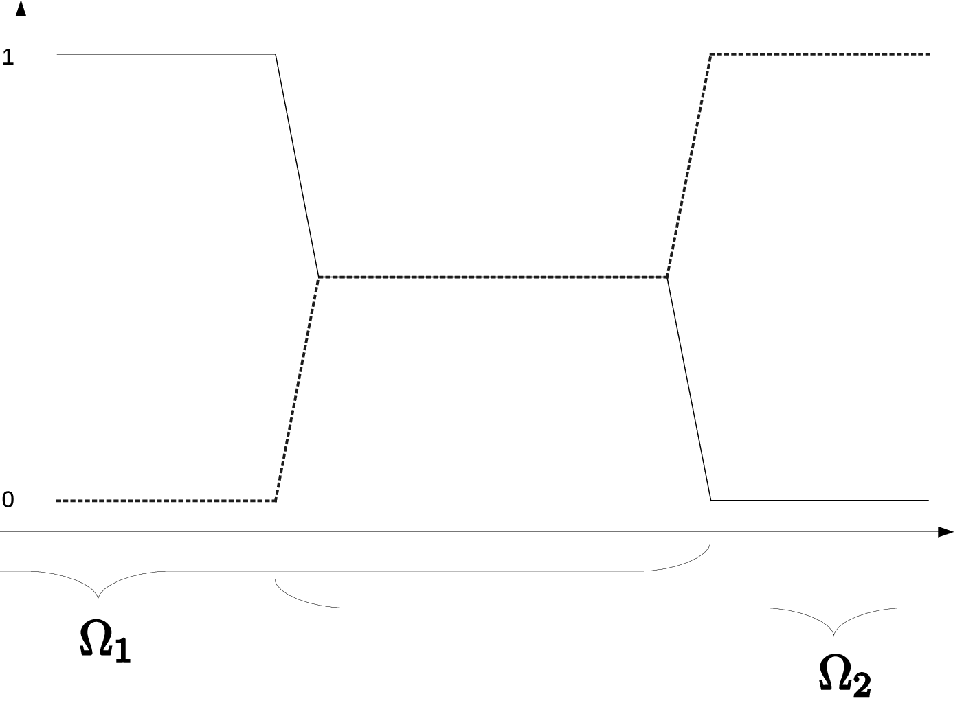
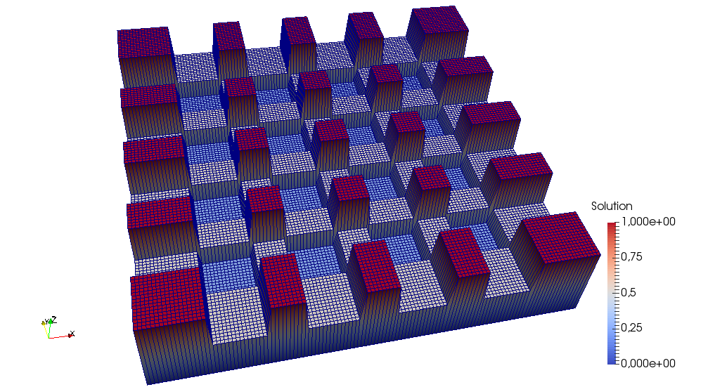

Figure 1 shows two examples of partitions of unity. It should be noted that implementing a smooth partition of unity for arbitrary subdomain arrangements can be challenging and in our tests we have not found this to have a large influence on the efficiency of the preconditioner. Using the partition of unity operators defined above, we can now state the definition of the GenEO coarse space. The space is constructed from the eigenvectors of a specific generalized eigenproblem representing the inequality required by the stable splitting.
For each subdomain , we define the generalized eigenproblem: Find such that
| (5) |
Note that the eigenproblems are local to their respective subdomain , i.e. they can be computed in parallel. To use them as a global basis they need to be extended to the entire domain using the partition of unity operators.
Definition 4 (GenEO coarse space)
For each subdomain , let be the eigenfunctions from the eigenproblem in (5) corresponding to the smallest eigenvalues. Then the GenEO coarse space is defined as
In [12] the following bound on the condition number of the matrix has been shown.
Theorem 3.1
For all , let the number of eigenvectors chosen in each subdomain be
where is a measure of the width of the overlap and . Then,
Thus the algorithm presented is provably independent of the number of subdomains and coefficient variations in the problem. Note that the choice of threshold by which the eigenvectors are selected is not unique. The threshold can be scaled to vary the condition number of the preconditioned system while retaining robustness. This allows us to control the total number of preconditioned CG iterations.
4 HPC Implementation of GenEO in Modern PDE Frameworks
When implementing the GenEO preconditioner in a PDE framework, the primary goal is to preserve the beneficial properties offered by its theoretical construction, namely:
- i)
High parallel scalability: Since the condition bound in Thm. 3.1 is independent of the number of subdomains we expect the implementation to yield high parallel scalability. The solution of the eigenproblems parallelizes trivially. However, care has to be taken when it comes to the communication necessary to set up the coarse matrix.
- ii)
Robustness with respect to problem parameters: While this is an inherent property of the preconditioner, some care is required in implementing the Dirichlet boundary conditions.
- iii)
Applicability to various types of PDEs: The theoretical framework only requires a symmetric positive definite bilinear form as in (1). This flexibility can be preserved in any numerical framework that is based on abstract bilinear forms. This is the case for many modern PDE frameworks, e.g. FEniCS [1], DUNE [4], or deal.ii [2].
In this section, we present a new implementation of the GenEO coarse space and preconditioner within DUNE (Distributed and Unified Numerics Environment), which fulfills these properties. This serves as a reference for the implementation, which is freely available as part of the dune-pdelab module [6] since version 2.6, as well as a general guideline for future implementations in other software packages. DUNE is a generic package that provides the user with key ingredients for solving any FEM problem. As an open source framework written using modern C++ programming techniques, it allows for modularity and reusability while providing HPC grade performance.
4.1 Prerequisites
Many of the components required to implement a two-level Schwarz method already exist within DUNE. In particular, we use the PDELab discretization module’s functionality to assemble stiffness matrices based on bilinear forms and for efficient communication across overlapping subdomains. The GenEO basis functions have support not restricted to individual elements, which makes the existing high-level components of PDELab unsuited for storing the coarse space. As part of this project, components facilitating such coarse spaces were fully integrated within the framework. Further, an efficient sequential solver for generalized eigenproblems is needed. Here, we choose ARPACK [8].
4.2 General Structure
The implementation in PDELab closely follows the structure of the previous section. All mathematical objects are represented as individual classes (see Fig. 2(b)). This separation of concerns leads to an easy to understand and well-structured code. Further, components are easily interchangeable when constructing related methods. In particular, the intricate process of constructing a global coarse space from per-subdomain basis functions is entirely contained in the class SubdomainProjectedCoarseSpace. Thus, the GenEO basis can easily be replaced by a different approach, as only the local basis functions need to be defined on that level.
4.3 Discrete Basis
To calculate GenEO basis functions we solve the discrete form of the eigenproblem in Def. 5, i.e.
where is the discretisation matrix assembled in the overlap region and is the discrete form of the partition of unity.
The matrix has to be assembled with Dirichlet constraints on the domain boundary as prescribed by the given PDE problem. However, in contrast to the matrices needed for the one-level component of the two-level additive Schwarz method, no Dirichlet constraints are imposed on subdomain boundaries.
For assembling , the same boundary conditions can be applied. However, additionally, the matrix should only be assembled on the overlap region. Internally these elements are determined by adding a vector of ones across subdomains and checking for results greater than one.
The matrices representing the partition of unity operator are diagonal and can be stored as vectors. Entries of corresponding to Dirichlet domain boundaries or processor boundaries should be zero, and in sum they should add up to one across subdomains. Such a partition of unity is generated by adding vectors of ones with one communication between subdomains.
4.4 Solving the Eigenproblem
As the eigenproblems are defined per-subdomain, the eigensolver itself does not need to run in parallel. However, solving larger problems requires an efficient iterative solver. A suitable choice is ARPACK [8].As the eigenvalues of interest for the GenEO coarse space are those of smallest magnitude, the Shift and Invert Spectral Transformation Mode supported by ARPACK is used. Instead of the generalized eigenproblem , ARPACK solves the transformed problem . The eigenvalues of the transformed problem are related to those of the original problem by and the eigenvectors are identical. In the transformed problem, the eigenvalues of the original problem whose absolute values are closest to are now the eigenvalues of largest magnitude, and can therefore be efficiently solved by the Krylov method. Choosing near zero, the method delivers the eigenvalues of smallest magnitude at good performance. Finally, in order to form the actual basis vectors, the eigenvectors are multiplied by and then normalized in the norm, as ARPACK delivers vectors of strongly varying norms.
4.5 Scalable Coarse Setup
Assembling the coarse matrix requires particular care, as it is a non-localized, not trivially scalable operation. Due to domain decomposition, the global matrix is only available in distributed form as matrices . Exploiting local support of basis functions, the coarse matrix breaks down into
We note that is zero for , leading to a sparse structure in . Therefore, all rows of associated to basis functions can be computed on the associated process locally while only requiring basis functions from adjacent subdomains. In the implementationmultiple basis functions are communicated in a single step.
The resulting blocks are combined into a matrix available on all processes, using direct MPI calls, while exploiting sparsity. Communication effort obviously increases with the dimension of . This is a direct consequence of how two-level preconditioners are designed, and a good balance between coarse space size and preconditioner performance must be found.
The restriction and prolongation operators and are also only available locally. In case of the restriction of a distributed vector , it holds
Each row can be computed by the process associated to , and the rows can be exchanged among all processes via MPI_Allgatherv. Again, the communication effort increases with the dimension of .
Finally, the prolongation of a global vector fulfills
Here, each part of the sum associated with a processor can be computed locally and combined by nearest-neighbor communication, scaling ideally.
5 Numerical Experiments
In this section we demonstrate the solvers salient features, including its high parallel scalability up to cores, its robustness to heterogeneous material parameterss and its applicability to different elliptic PDEs. With exception of the final large-scale experiment all numerical examples in this section have been computed using the Balena HPC cluster of the University of Bath. Balena consists of nodes each with two -core Intel Xeon E5-2650v2 Ivybridge processors, each running at GHz and giving a total of available cores.
5.1 GenEO Basis on Highly Structured Problems
With clearly structured problems, it can be visually seen that the GenEO coarse space systematically picks up inclusions or channels in the parameter distribution. In Figure 3 the coarse approximation error is shown for a Darcy problem on a square domain. Dirichlet conditions are set to one at the top and zero at the bottom, Neumann conditions are set at the remaining boundary and a high-contrast parameter distribution with jumps and channels as shown on the left. We see that each inclusion has an effect on the approximation error. Adding additional eigenvectors from each subdomain to the coarse basis removes some of those error sources, the next eigenvectors pick up the skyscrapers and with only 4 eigenvectors per subdomain most channels are picked up. A total of coarse basis functions is enough to almost entirely solve the given problem.
5.2 Demonstration of Robustness
Robustness with respect to parameter contrast can be demonstrated solving the same Darcy problem as in section 5.1. We choose a subdomain decomposition into 8 by 8 squares, a two-cell overlap region diameter and a total of 800 elements in each direction. Figure 4 (left) shows the resulting condition number for increasing contrast when setting up a GenEO basis with various numbers of eigenvectors per subdomain. Clearly, the asymptotic robustness guaranteed by the analysis is achieved in practice.
When running the same setup with a parameter distribution of 40 horizontal equally thick layers, it becomes clear from Figure 4 (right) that robustness is achieved exactly at four eigenvectors per subdomain. That stems from the fact that four coarse basis functions (together with the contribution of the one-level Schwarz method) are sufficient to represent the five layers contained in that subdomain. Similar relations can be observed with other strongly structured parameter distributions as well.
5.3 Comparison to other solvers
In this section we compare the performance of various preconditioned CG solvers. For this test we consider a flat composite plate of size . The laminate is made up of composite layers stacked in a sequence of different angles, refered to as a stacking sequence. The composite layers are seperated by very thin layers of resin. There is a large jump in material strength between the composite and resin layer and due to the rotated layers the anisotropy cannot be grid aligned. We discretise with quadratic, 20-node serendipity elements to avoid shear locking and use full Gaussian integration.
In Table 1 we compare the convergence of several iterative solvers. We record the condition number, the dimension of the coarse space if applicable and the number of CG iterations required to achieve a residual reduction of . As expected the iteration counts increase steadily with the number of subdomains when no coarse space is used. In contrast, the iterations and the condition number estimates remain constant for the GenEO preconditioner as predicted by Thm. 3.1.
| 1-level | GenEO | BoomerAMG | ||||
|---|---|---|---|---|---|---|
| iter. | iter. | dim() | iter. | |||
| 4 | 89 | 79,735 | 16 | 10 | 78 | 258 |
| 8 | 97 | 84,023 | 15 | 9 | 126 | 258 |
| 16 | 107 | 98,579 | 16 | 10 | 182 | 257 |
| 32 | 158 | 226,871 | 16 | 9 | 526 | 263 |
To demonstrate the efficiency of this approach we also compared with two different implementations of AMG. The implementation included in dune-istl has not originally been designed for composite application, and in its current form it does not seem to be robust, especially in parallel [9]. We applied this solver in its block version and measured strength of connection between two blocks for the aggregation procedure in the Frobenius norm. As a smoother we applied two SSOR iterations. In the test setup used here the dune-istl AMG converges very slowly or not at all, thus we do not include it in Table 1. We include results for BoomerAMG [15]. Here we retained the defaults for most parameters (HMIS coarsening without aggressive refinement levels and a hybrid Gauss-Seidel smoother). As recommended for elasticity problems we used blocked aggregation with block size corresponding to the spatial dimension. A strong threshold of was chosen after testing values in the range from to . Due to a lower setup cost the boomerAMG solver is faster in actual CPU time than the GenEO solver in this small test case. However, for more complex geometries, boomerAMG does not perform very well and in our tests it does not scale beyond about cores in composite applications [7].
5.4 Industrially-motivated Example: Wingbox
In this section we describe an industrially motivated example in which we asses the strength of an airplane wingbox with a small localised wrinkle defect in one corner. Wrinkle defects often form during the manufacturing process and lead to strong local stress concentrations, which may cause premature failure [9, 10]. More details on this test setup can be found in [7].
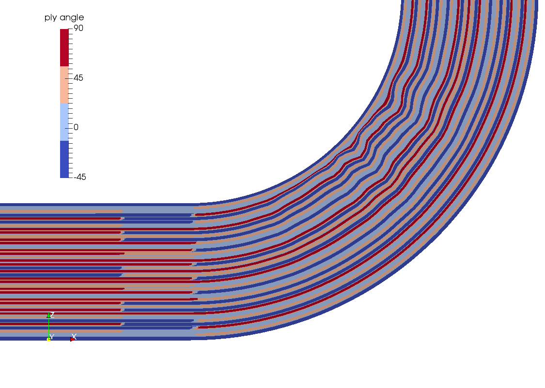
We model a single bay of a wingbox of width m, height cm, length m and internal radius of the corners mm, as shown in Figure 5 (left). As in a typical aerospace application, the stacking sequence differs in the covers (top and bottom), corners and in the spar (sides). The changing stacking sequence is shown in Figure 5 (right). In total the laminate is made up of fibrous layers and resin layers. One of the corner radii contains a localised wrinkle with a parametrisation matching an observed defect in a CT-Scan of a real corner section, for further details see [10].

Two forms of loading are applied, an internal pressure of MPa, arising from the fuel, is applied to the internal surface and a thermal pre-stress induced by the manufacturing process is imposed. The influence of ribs that constrain the wingbox in the direction are approximated by clamping all degrees of freedom at one end and tying all other degrees of freedom at the other end using a multipoint constraint.
To demonstrate the effectiveness of the GenEO solver we carry out a weak scaling and a strong scaling experiment. The experiments in this section were performed using the UK national HPC cluster Archer, which consists of Cray XC30 nodes with two GHz, -core E5-2697 v2 CPUs each.
For the weak scaling experiment we refine the mesh, doubling the number of elements as we double the number of cores. Tab. 2 (left) contains the number of degrees of freedom, iteration numbers for the preconditioned CG, an estimate of the condition number of the discretisation matrix , the dimension of the coarse space , as well as the total run time for each test. The weak scaling of the iterative CG solver with GenEO preconditioner is indeed almost optimal up to at least cores. We note that as shown in Thm. 3.1 the condition number remains bounded. As expected we observe a clear connection between the number of iterations and the condition number.
Tab. 2 (right) shows a strong-scaling experiment. The iterative CG solver with GenEO preconditioner scales almost optimally to at least cores. Memory constraints prevented tests with fewer than cores. Tab. 2 shows that the number of iterations indeed remains almost constant. The last column gives the parallel efficiency, it remains high up to cores.
| DOF | iter. | Time (sec) | |||
|---|---|---|---|---|---|
| 480 | 156 | 445 | 5025 | 734 | |
| 960 | 154 | 421 | 7840 | 806 | |
| 1920 | 152 | 322 | 18752 | 800 | |
| 3840 | 144 | 287 | 29444 | 772 | |
| 7680 | 132 | 303 | 50930 | 764 | |
| 15360 | 102 | 245 | 94527 | 845 |
| elements/ | it. | Time (sec) | efficiency | ||
|---|---|---|---|---|---|
| 2880 | 3132 | 18843 | 167 | 2906 | 1.00 |
| 3840 | 2340 | 26333 | 153 | 1766 | 1.23 |
| 7680 | 2008 | 52622 | 132 | 1057 | 0.83 |
| 11320 | 1392 | 78233 | 162 | 706 | 1.01 |
6 Acknowledgements
This work was supported by an EPSRC Maths for Manufacturing grant (EP/K031368/1). This research made use of the Balena High Performance Computing Service at the University of Bath. This work used the ARCHER UK National Supercomputing Service (http://www.archer.ac.uk).
References
- [1] Alnæs, M.S., Blechta, J., Hake, J., Johansson, A., Kehlet, B., Logg, A., Richardson, C., Ring, J., Rognes, M.E., Wells, G.N.: The fenics project version 1.5. Archive of Numerical Software 3(100) (2015). https://doi.org/10.11588/ans.2015.100.20553
- [2] Alzetta, G., Arndt, D., Bangerth, W., Boddu, V., Brands, B., Davydov, D., Gassmoeller, R., Heister, T., Heltai, L., Kormann, K., Kronbichler, M., Maier, M., Pelteret, J.P., Turcksin, B., Wells, D.: The deal.II library, version 9.0. Journal of Numerical Mathematics 26(4), 173–183 (2018). https://doi.org/10.1515/jnma-2018-0054
- [3] Babuška, I., Caloz, G., Osborn, J.E.: Special finite element methods for a class of second order elliptic problems with rough coefficients. SIAM Journal on Numerical Analysis 31(4), 945–981 (1994)
- [4] Bastian, P., Blatt, M.: On the generic parallelisation of iterative solvers for the finite element method. Int. J. Computational Science and Engineering 4(1), 56–69 (2008)
- [5] Bastian, P., Blatt, M., Dedner, A., Engwer, C., Klöfkorn, R., Kornhuber, R., Ohlberger, M., Sander, O.: A generic grid interface for parallel and adaptive scientific computing. part ii: Implementation and tests in dune. Computing 82(2-3), 121–138 (2008)
- [6] Bastian, P., Heimann, F., Marnach, S.: Generic implementation of finite element methods in the distributed and unified numerics environment (dune). Kybernetika 46(2), 294–315 (2010)
- [7] Butler, R., Dodwell, T., Reinarz, A., Sand hu, A., Scheichl, R., Seelinger, L.: dune-composites – an open source, high performance package for solving large-scale anisotropic elasticity problems. arXiv e-prints arXiv:1901.05188 (Jan 2019)
- [8] Lehoucq, R.B., Sorensen, D.C., Yang, C.: Arpack users guide: Solution of large scale eigenvalue problems by implicitly restarted arnoldi methods. (1997)
- [9] Reinarz, A., Dodwell, T., Fletcher, T., Seelinger, L., Butler, R., Scheichl, R.: Dune-composites - A new framework for high-performance finite element modelling of laminates. Composite Structures 184, 269–278 (2018)
- [10] Sandhu, A., Reinarz, A., Dodwell, T.: A bayesian framework for assessing the strength distribution of composite structures with random defects. Composite Structures 205 (08 2018). https://doi.org/10.1016/j.compstruct.2018.08.074
- [11] Smith, B.F., Bjørstad, P.E., Gropp, W.: Domain decomposition. Cambridge Univ. Press, Cambridge [u.a.] (1996), includes bibliographical references
- [12] Spillane, N., Dolean, V., Hauret, P., Nataf, F., Pechstein, C., Scheichl, R.: Abstract robust coarse spaces for systems of PDEs via generalized eigenproblems in the overlaps. Springer Berlin Heidelberg, Berlin/Heidelberg (2014)
- [13] Spillane, N., Dolean, V., Hauret, P., Nataf, F., Pechstein, C., Scheichl, R.: A robust two-level domain decomposition preconditioner for systems of PDEs. Elsevier B.V (2011)
- [14] Toselli, A., Widlund, O.: Domain decomposition methods - algorithms and theory. Springer series in computational mathematics, Springer, Berlin ; Heidelberg [u.a.] (2005)
- [15] Yang, U.M., Henson, V.E.: BoomerAMG: A parallel algebraic multigrid solver and preconditioner. Applied Numerical Mathematics 41(1), 155–177 (2002)