³The Higgs Centre for Theoretical Physics, University of Edinburgh,
JCMB, KB, Mayfield Rd, Edinburgh EH9 3JZ, Scotland
⁴Tif Lab, Dipartimento di Fisica, Università di Milano and
INFN, Sezione di Milano, Via Celoria 16, I-20133 Milano, Italy
⁵Cavendish Laboratory, University of Cambridge, Cambridge CB3 0HE, United Kingdom
⁶Dipartimento di Fisica G. Occhialini, U2, Università degli Studi di Milano-Bicocca, Piazza della Scienza, 3, 20126 Milano, Italy and
INFN, Sezione di Milano-Bicocca, 20126, Milano, Italy
⁷DAMTP, University of Cambridge, Wilberforce Road,
Cambridge, CB3 0WA, United Kingdom

Abstract

We formulate a general approach to the inclusion of theoretical uncertainties, specifically those related to the missing higher order uncertainty (MHOU), in the determination of parton distribution functions (PDFs). We demonstrate how, under quite generic assumptions, theory uncertainties can be included as an extra contribution to the covariance matrix when determining PDFs from data. We then review, clarify, and systematize the use of renormalization and factorization scale variations as a means to estimate MHOUs consistently in deep inelastic and hadronic processes. We define a set of prescriptions for constructing a theory covariance matrix using scale variations, which can be used in global fits of data from a wide range of different processes, based on choosing a set of independent scale variations suitably correlated within and across processes. We set up an algebraic framework for the choice and validation of an optimal prescription by comparing the estimate of MHOU encoded in the next-to-leading order (NLO) theory covariance matrix to the observed shifts between NLO and NNLO predictions. We perform a NLO PDF determination which includes the MHOU, assess the impact of the inclusion of MHOUs on the PDF central values and uncertainties, and validate the results by comparison to the known shift between NLO and NNLO PDFs. We finally study the impact of the inclusion of MHOUs in a global PDF determination on LHC cross-sections, and provide guidelines for their use in precision phenomenology. In addition, we also compare the results based on the theory covariance matrix formalism to those obtained by performing PDF determinations based on different scale choices.

1 Introduction

An accurate estimate of the uncertainty in Standard Model (SM) predictions is a crucial ingredient for precision phenomenology at the Large Hadron Collider (LHC). Now, and for several years to come [1, 2], theoretical uncertainties for hadron collider processes are dominated by the missing higher order uncertainty (MHOU) in perturbative QCD calculations, usually estimated by scale variation, and by parton distribution function (PDF) uncertainties. Of course, PDFs summarize the information on the nucleon structure extracted from other SM processes [3]: effectively, PDFs provide a way of obtaining a prediction for a given process in terms of other processes. This way of thinking about PDFs immediately shows that MHOUs are present not only in the perturbative prediction for a particular process, but also in the underlying processes used for the PDF determination.

Current PDF uncertainties essentially only include the propagated uncertainty arising from statistical and systematic uncertainties in the experimental data used in their determination. Methodological uncertainties related for example to the choice of functional form for the PDFs, or the fitting methodology employed, can be kept under control using closure tests [4], and with care can be made negligible in the data region. Parametric uncertainties, such as those related to the value of the strong coupling $\alpha_{s}(m_{Z})$ or the charm mass $m_{c}$ can be included by performing fits for a range of parameters. However up until now MHOUs have never been included in a PDF fit: what is usually called the “PDF uncertainty” does not include the MHOU in the theoretical calculations used for PDF determination, and, more generally, does not typically include any source of theory uncertainty.

Historically, this is related to the fact that MHOUs have always been considered as likely to be small in comparison to other PDF uncertainties, especially since NNLO PDFs have become the default standard. However, it is clear that as PDF uncertainties become smaller and smaller, at some point MHOUs will become significant. In the most recent NNPDF set, NNPDF3.1 [5], PDF uncertainties at the electroweak scale can be as low as 1%. Given that the typical size of MHOU on NNLO QCD processes is at the percent level (see e.g. [6]) their neglect seems difficult to justify a priori.

Besides contributing to the overall size of PDF uncertainty, more subtly the MHOU might affect the relative weights of different datasets included in the fit: a dataset which is accurately described by NNLO theory because it has small MHOU should in principle carry more weight than one which is poorly described because it has large MHOU. The neglect of MHOUs might thus be biasing current global PDF fits.

It is the purpose of this paper to set up a general formalism for the inclusion of theoretical uncertainties, specifically MHOUs, in PDF determinations, and then to perform a first phenomenological exploration of their impact on LHC phenomenology. The development of this treatment of MHOUs will involve three main ingredients. The first is the formulation of a general theory for the inclusion in PDF fits of generic theoretical uncertainties, of which MHOUs are a particular case. The second is the choice of a specific method for estimating the MHOU in each of the cross-sections that enter the PDF fit. The third is the construction of a set of tools for the validation of this methodology, to check that the MHOU is being correctly estimated.

The first ingredient in our approach is common to any kind of theory uncertainty: theory uncertainties include not only MHOUs, but also any other aspect in which the theory used in order to obtain predictions for the physical processes that enter the PDF fit is incompletely known. These include higher twists (see Refs.[7, 8] and Ref. therein) and other power-suppressed corrections, nuclear corrections when nuclear targets are involved (see Refs.[9, 10] and Ref. therein), final state corrections for non-inclusive processes, and so forth. All of these uncertainties are only meaningful in a Bayesian sense: there is only one correct value of the next-order perturbative correction, not a distribution of values. They thus necessarily involve a process of informed estimation or guesswork: the only way to actually know the size of, say, a missing higher order correction, is to calculate it.

We will show by adopting a Bayesian point of view, and assigning a Gaussian probability distribution to the expected true value of the theory calculation, that the impact of any missing theoretical contribution can be encoded as an additive contribution to the experimental covariance matrix used in the PDF fit [11]. The combination is additive because experimental and theoretical uncertainties are by their nature independent, and are thus combined in quadrature. In a global fit, theoretical uncertainties can be strongly correlated not only across data points within a given experiment, but also between different experiments, and even different processes, so we need a theoretical covariance matrix which includes all these correlations across all the datasets included in the fit.

This then immediately raises the issue of choosing a meaningful way to estimate the MHOU, which in particular incorporates these correlations. The standard way of estimating MHOUs in perturbative QCD calculations is to perform a variation of the renormalization and factorization scales, denoted as $\mu_{r}$ and $\mu_{f}$ respectively, with various choices for the range and combination of variations existing. While the shortcomings of this method are well known, and various alternatives have been discussed [12, 13, 14], this remains the default and most widely used option. In the present context, its main advantage is its universality (it can be applied in the same way to any of the processes used in the fit), and the way in which it implicitly incorporates correlations (for example predictions for data points in the same process which are kinematically close will be automatically correlated), even across different processes (through the PDFs, which are the same in every process). Thus while in principle our covariance matrix formalism allows for the inclusion of any method for estimating MHOUs in a PDF determination, here we will specifically use scale variation.

In order to do this, we need to examine systematically the underpinnings of scale variation as a means to estimate theory uncertainties, since different definitions of scale variation have been used in different contexts. Indeed, the standard definitions of renormalization and factorization scale typically used for deep-inelastic scattering and hadronic collisions are not the same. Because PDF fits include both types of processes, it is important to understand in detail how these definitions relate to each other, in order to be able to correlate the scale variations in a meaningful way. Specifically, we will show that one may estimate the MHOU for any process by combining two independent scale variations: one to estimate the MHOU in the perturbative evolution of the PDFs (missing higher orders in the DGLAP splitting functions), and the other to estimate the MHOU in the perturbative calculation of the partonic cross-sections (missing higher orders in the hard-scattering matrix elements).

Once the scales to be varied are understood, the remaining task is to choose a particular prescription to be used to construct the theoretical covariance matrix. In estimating MHOUs for a given process, the most commonly adopted option is the so-called seven-point envelope prescription, in which $\mu_{r}$ and $\mu_{f}$ are independently varied by a factor of two about the central choice while ensuring that $1/2\leq\mu_{r}/\mu_{f}\leq 2$ , and the MHOU is then taken as the envelope of the results. For our purposes this is insufficient: rather than taking an envelope, we wish to contruct a covariance matrix out of the scale variations. In particular, because theoretical uncertainties are correlated across processes (through the evolution of the PDFs), we need a prescription for determining the entries of the covariance matrix both within a single process and across pairs of processes.

We will discuss in detail a variety of options to achieve this, based on a general “ $n$ -point prescription”. These options will differ from each other in the choice of the number of independent variations, the directions of such variations in the $(\mu_{r},\mu_{f})$ plane, and the way the variations are correlated (or not) across different processes.

The validation of these point prescriptions, and the choice of the optimal one to be used for PDF determinations is a nontrivial problem, which however admits an elegant solution. The validation can be performed at NLO, by comparing the estimate of the MHOU encoded in the theory covariance matrix to the known next (NNLO) order correction. The problem is then to compare the probability distribution of expected higher-order results to the unique answer given by the NNLO calculation. The solution to this problem is to view the set of shifts between the NLO and NNLO computations for all the processes under consideration as a vector, with one component for each of the data points. The theory covariance matrix corresponding to each prescription then defines a one-sigma ellipsoid in a subspace of this space. The validation is performed by projecting the shift vector into the ellipsoid: if the theory covariance matrix gives a sensible estimate of the MHOU at NLO, the shift vector will lie almost entirely within the ellipsoid. Using this strategy, we will validate a variety of scale variation prescriptions on a similar dataset to that of the global NNPDF3.1 analysis. Since the dimension of the space of datapoints is typically two orders of magnitude higher than the dimension of the subspace of the ellipsoid, this is a highly nontrivial test.

Once a prescription has been selected and used to construct the theory covariance matrix, it is possible to perform a PDF fit based on it. Within the NNPDF methodology, an ensemble of PDF replicas is fitted to data replicas. Data replicas are generated in a way which reflects the uncertainties and correlations of the underlying data, as encoded in their covariance matrix. The best-fit PDF replica for each data replica is then determined by minimizing a figure of merit ( $\chi^{2}$ ) which is computed using the covariance matrix. As mentioned, and as we shall show in Sect. 2, the theory contribution appears as an independent contribution to the total covariance matrix, uncorrelated with the experimental one and simply added to it. Therefore, once the covariance matrix is supplemented by an extra theory contribution coming from MHOUs, this should be treated on the same footing as any other contribution, and it will thus affect both the data replica generation, and the fitting of PDF replicas to data replicas.

Qualitatively, one may expect the inclusion of the MHOU in the data replica generation to increase the spread of the data replicas, and thus lead in itself to an increase in overall PDF uncertainties. On the other hand the inclusion of the MHOU in the fitting might also reduce tensions within the fit due to the imperfection of the theory and, since these are highly correlated, result in significant shifts in central values, and overall a better fit with reduced uncertainties. The combined effect of including the MHOU in both the data generation and the fitting is thus not at all obvious.

We will investigate these effects by performing PDF determinations in which MHOUs are included in either, or both, the replica generation and the PDF replica fitting. Once again, results can be validated at NLO by comparing NLO PDFs determined with the theory covariance matrix to NNLO PDFs. A successful validation should show that the best-fit NLO PDF moves towards the central NNLO result upon inclusion of the theory covariance matrix in both replica generation and fitting, due to a relaxation of tensions in the NLO fit, and that the NNLO PDF differs from the NLO PDF by an amount which is correctly estimated by the NLO uncertainty band. As we shall see, this is indeed the case, and in fact it will turn out that often the uncertainty band does not increase or even decreases upon inclusion of the theory covariance matrix.

Having determined PDFs which now account for the MHOU associated to the processes that enter the fit, the natural questions which then arise are what is their impact, and more generallly how they should be used for precision LHC phenomenology. In order to address the first question, we will compute predictions with MHOUs for typical LHC standard candle processes, both with and without including the MHOU in the PDF, and provide a first phenomenological exploration and assessment of the impact of these uncertainties.

The second question is not entirely trivial and we will address it in detail. Indeed, scale variation is routinely performed in order to estimate the MHOU in theoretical predictions for hadron collider processes. Clearly, when obtaining a prediction, we should avoid double counting a MHOU which has already been included in the PDF. Instances in which this might happen include not only the trivial situation in which a prediction is obtained for a process which has already been used for PDF determination, but also the somewhat more subtle situation in which the MHOU in the PDF and the observable which is being predicted are correlated through perturbative evolution [15]. We will discuss this situation, and provide guidelines for the usage of PDFs with MHOUs.

This paper is broadly divided into two main parts. In the first part, we construct a general formalism for the inclusion of theory uncertainties and specifically MHOUs in PDF determination, and show how to construct and validate a theory covariance matrix. In the second part, we perform a first investigation of the phenomenological implications of these theory uncertainties. The structure of the paper is the following: in Sect. 2 we show, using a Bayesian approach, that under certain assumptions any type of theory uncertainty can be included as a contribution to the covariance matrix. In Sect. 3 we summarize the theory of scale variation and use it to review, compare and systematize different definitions which have been used in the literature. In Sect. 4 we then formulate a number of “point prescriptions” for the theory covariance matrix, both for a single process, and also to account for correlations between a pair of processes. In Sect. 5 we compute the theory covariance matrix for a variety of prescriptions, we test them against known higher order corrections, and use this comparison to select an optimal prescription.

We then move to the second, more phenomenological, part of the paper. The centerpiece of this section is the determination of NLO PDF sets with MHOU, presented in Sect. 6. We first only include deep-inelastic scattering data (DIS-only fit), and then adopt a global data set, which is compared to PDFs without MHOU, and validated against NNLO PDFs. In Sect. 7 we present initial studies of the phenomenological impact of the inclusion of MHOUs in PDFs for representative LHC processes. Finally in Sect. 8 we provide guidelines for the usage of PDFs with MHOU, in particular concerning the combination of the PDF uncertainties with the MHOU on the hard matrix element, and present the delivery of the PDF sets produced in this work.

Two appendices contain further studies and technical details. In Appendix A we provide additional details concerning the procedure adopted to diagonalise the theory covariance matrix. Then in Appendix B we study another possible validation of the results of Sect. 6, by comparing PDFs with MHOUs to the PDFs obtained by adopting different choices of renormalization and factorization scales in the PDF determination. Families of fits which only differ in choices of scale have never been carried out before and will be presented here for the first time. Whereas they do not necessarily give a fair estimate of the MHOU on PDFs, they surely do provide an indication of the expected impact of scale variation on PDFs, and the pattern of MHOU correlations.

A concise discussion of the main results of this work was presented in Ref. [16], of which this paper represents the extended companion.

2 A theoretical covariance matrix

Parton distribution functions are determined from a set of $N_{\rm dat}$ experimental data points, which we represent by an $N_{\rm dat}$ -dimensional vector $D_{i}$ , $i=1,\ldots,N_{\rm dat}$ . These data points have experimental uncertainties that may be correlated with each other, and this information is encoded in an experimental covariance matrix $C_{ij}$ . This covariance matrix may be block-diagonal if some sets of data are uncorrelated. Each experimental data point has associated with it a “true” value ${\cal T}_{i}$ — the value given by Nature — whose determination is the goal of the experiment. Since the experimental measurements are imperfect, they cannot determine ${\cal T}$ exactly, but they can be used to estimate the Bayesian probability of a given hypothesis for ${\cal T}$ . Assuming that the experimental results are Gaussianly distributed about this hypothetical true value, the conditional probability for the true values ${\cal T}$ given the measured cross-sections $D$ is

P({\cal T}|D)=P(D|{\cal T})\propto\exp\big(-\hbox{${{1}\over{2}}$}({\cal T}_{i}-D_{i})C_{ij}^{-1}({\cal T}_{j}-D_{j})\big),

(2.1)

up to an overall normalization constant. Note that this tacitly assumes equal priors for both $D$ and ${\cal T}$ .

Of course the true values ${\cal T}_{i}$ are unknown. However we can calculate theoretical predictions for each data point $D_{i}$ , which we denote by $T_{i}$ . These predictions are computed using a theory framework which is generally incomplete: for example because it is based on the fixed-order truncation of a perturbative expansion, or because it excludes higher-twist effects, or nuclear effects, or some other effect that is difficult to calculate precisely. Furthermore, these theory predictions $T_{i}$ depend on PDFs, evolved to a suitable scale also using incomplete theory. While the theory predictions may correspond to a variety of different observables and processes, they all depend on the same underlying (universal) PDFs.

We now assume, in the same spirit as when estimating experimental systematics, that the true values ${\cal T}_{i}$ are centered on the theory predictions $T_{i}$ , and Gaussianly distributed about the theory predictions, with which they would coincide if the theory were exact and the PDFs were known with certainty. The conditional probability for the true values ${\cal T}$ given theoretical predictions $T$ is then

P({\cal T}|T)=P(T|{\cal T})\propto\exp\big(-\hbox{${{1}\over{2}}$}({\cal T}_{i}-T_{i})S_{ij}^{-1}({\cal T}_{j}-T_{j})\big),

(2.2)

again up to a normalization constant, where $S_{ij}$ is a “theory covariance matrix”, to be estimated in due course.

PDFs are determined by maximizing the probability of the theory given the data $P(T|D)$ , marginalised over the true values ${\cal T}$ which of course remain unknown. Now using Bayes’ theorem

P({\cal T}|DT)P(D|T)=P(D|{\cal T}T)P({\cal T}|T)\,.

(2.3)

Moreover, since the experimental data do not depend on the theorists’ calculations $T$ , but only on the ‘truth’ ${\cal T}$ ,

P(D|{\cal T}T)=P(D|{\cal T}).

(2.4)

Then because by construction $\int\!D^{N}{\cal T}\,P({\cal T}|TD)=1$ ,

P(D|T)=\int\!D^{N}{\cal T}\,P({\cal T}|D)P({\cal T}|T)\,,

(2.5)

where the $N$ -dimensional integral is over all of the possible values of ${\cal T}_{i}$ . The probability of the experimental data $D$ is now conditional on the theory $T$ because we have marginalised over the underlying ‘truth’ ${\cal T}$ , which is common to both.

Writing the difference between the true ${\cal T}_{i}$ and the actual $T_{i}$ values of the theory prediction as

\Delta_{i}\equiv{\cal T}_{i}-T_{i}\,,

(2.6)

we can change variables of integration to convert the integral over ${\cal T}_{i}$ into an integral over the shifts $\Delta_{i}$ : using the Gaussian hypotheses Eqns. (2.1) and (2.2), Eq. (2.5) becomes that

P(D|T)\propto\int\!D^{N}\Delta\,\exp\big(-\hbox{${{1}\over{2}}$}\left(D_{i}-T_{i}-\Delta_{i}\right)C_{ij}^{-1}\left(D_{j}-T_{j}-\Delta_{j}\right)-\hbox{${{1}\over{2}}$}\Delta_{i}S_{ij}^{-1}\Delta_{j}\big).

(2.7)

The Gaussian integrals can now be performed explicitly. Adopting a vector notation in order to make the algebra more transparent, we rewrite the exponent as

	$\displaystyle(D-T-\Delta)^{T}C^{-1}(D-T-\Delta)+\Delta^{T}S^{-1}\Delta\qquad\qquad\qquad$	(2.8)
$\displaystyle=$	$\displaystyle\Delta^{T}(C^{-1}+S^{-1})\Delta-\Delta^{T}C^{-1}(D-T)-(D-T)^{T}C^{-1}\Delta+(D-T)^{T}C^{-1}(D-T)$
$\displaystyle=$	$\displaystyle(\Delta-(C^{-1}+S^{-1})^{-1}C^{-1}(D-T))^{T}(C^{-1}+S^{-1})(\Delta-(C^{-1}+S^{-1})^{-1}C^{-1}(D-T))$
$\displaystyle-$	$\displaystyle(D-T)^{T}C^{-1}(C^{-1}+S^{-1})^{-1}C^{-1}(D-T)+(D-T)^{T}C^{-1}(D-T),$

where we used the fact that both $C$ and $S$ are symmetric matrices, and in the last line we completed the square. Integrating over $\Delta$ , ignoring the normalization, Eq. (2.7) then becomes

P(T|D)=P(D|T)\propto\exp\big(-\hbox{${{1}\over{2}}$}(D-T)^{T}(C^{-1}-C^{-1}(C^{-1}+S^{-1})^{-1}C^{-1})(D-T)\big)\,.

(2.9)

However

(C^{-1}+S^{-1})^{-1}=(C^{-1}(C+S)S^{-1})^{-1}=S(C+S)^{-1}C,

(2.10)

so that

\displaystyle\begin{split}C^{-1}&-C^{-1}(C^{-1}+S^{-1})^{-1}C^{-1}=C^{-1}-C^{-1}S(C+S)^{-1}\\ &=(C^{-1}(C+S)-C^{-1}S)(C+S)^{-1}=(C+S)^{-1}.\end{split}

(2.11)

Restoring the indices, we thus find the simple result

P(T|D)\propto\exp\big(-\hbox{${{1}\over{2}}$}(D_{i}-T_{i})(C+S)_{ij}^{-1}(D_{j}-T_{j})\big).

(2.12)

Comparison of Eq. (2.12) with Eq. (2.1) indicates that when replacing the true ${\cal T}_{i}$ by the theoretical predictions $T_{i}$ in the expression of the $\chi^{2}$ of the data, the theoretical covariance matrix $S_{ij}$ should simply be added to the experimental covariance matrix $C_{ij}$ [11]. In effect this implies that, at least within this Gaussian approximation, when determining PDFs theoretical uncertainties can be treated simply as another form of experimental systematic: it is an additional uncertainty to be taken into account when trying to find the truth from the data on the basis of a specific theoretical prediction. The experimental and theoretical uncertainties are added in quadrature because they are in principle uncorrelated.

In the case for which theoretical uncertainties can be neglected, i.e. if $S_{ij}\to 0$ , then $P({\cal T}|T)$ in Eq. (2.2) becomes proportional to $\delta^{N}({\cal T}_{i}-T_{i})$ . As a result, in this case Eq. (2.12) reduces to Eq. (2.1) with ${\cal T}_{i}$ replaced by the predictions $T_{i}$ . This shows that Eq. (2.12) remains true even if $S_{ij}$ has zero eigenvalues and is thus not invertible. Note however that by construction $C_{ij}$ is positive definite, since any experimental measurement always has uncorrelated statistical uncertainties due to the finite number of events, so $(C+S)_{ij}$ will always be invertible.

The question remains of how to estimate the theory covariance matrix, $S_{ij}$ . The Gaussian hypothesis Eq. (2.2) implies that

S_{ij}=\big\langle({\cal T}_{i}-T_{i})({\cal T}_{j}-T_{j})\big\rangle=\big\langle\Delta_{i}\Delta_{j}\big\rangle,

(2.13)

where the average is taken over the true theory values ${\cal T}$ using the probability distribution $P({\cal T}|T)$ , and $\langle\Delta_{i}\rangle=0$ consistent with the assumption that the probability distribution of the truth ${\cal T}$ is centred on the theoretical calculation $T$ . In practice however the formal definition Eq. (2.13) is not very helpful: we need some way to estimate the shifts $\Delta_{i}$ — ‘nuisance parameters’, in the language of systematic error determination — in a way that takes into account the theoretical correlations between different kinematic points within the same dataset, between different datasets measuring the same physical process, and between datasets corresponding to different processes (with initial state hadrons). Note that theory correlations will always be present even for entirely different processes, through the universal parton distributions: the only processes with truly independent theoretical uncertainties are those with only leptons in the initial state, which are of course irrelevant for PDF determination.

The most commonly used method of estimating the theory corrections due to MHOUs, which can naturally incorporate all these theoretical correlations, is scale variation. This method is reviewed in Sect. 3 in general terms and then used in Sect. 4 in order to formulate specific prescriptions for constructing the theory covariance matrix $S_{ij}$ . Other approaches which have been discussed in the literature involve estimating MHOUs based on the behaviour of the known perturbative orders [12, 13, 14]; however, at least at present, these do not appear to provide a formalism which is sufficiently well-established, and of appropriately general applicability. We emphasize however that the formalism presented in this section is independent of the specific method adopted to estimate the correlated theory shifts $\Delta_{i}$ that enter Eq. (2.13).

3 MHOUs from scale variations

The variation of the renormalization and factorization scales is the most popular approach for estimating missing higher order uncertainties (MHOUs) in QCD perturbative calculations. It has a number of advantages: it naturally incorporates renormalization group (RG) invariance, thereby ensuring that as the perturbative order increases, estimates of MHOU decrease; the same procedure can be used for any perturbative process, since the scale dependence of the strong coupling $\alpha_{s}(\mu^{2})$ and of PDFs is universal; the estimates of MHOU it produces are smooth functions of the kinematics, and thereby correctly incorporate the strong correlations in nearby regions of phase space; and correlations between different processes due to universal ingredients such as PDFs can be easily incorporated. Its drawbacks are also well known: there is no unique principle to determine the specific range of the scale variation (nor even the precise central scale to be adopted); and it misses uncertainties associated with new singularities or color structures present at higher orders but missing at lower orders. The former problem may be dealt with, at least qualitatively, by validating a given range in situations where the next order corrections are known. We will attempt such a validation in this paper. The latter problem is more challenging, requiring resummation in the case of unresummed logarithms, or other methods of estimating new types of corrections, and it is unclear whether or not it admits a general solution.

While scale variation has been discussed many times in a variety of contexts, there is no standard, commonly accepted formulation of it, and specifically none that can be applied to both electroproduction and hadroproduction processes, as we need to do if we wish to use scale variation in the context of global PDF analyses. In fact, it turns out that the most commonly adopted approaches to scale variation differ, typically according to the nature of the process which is being considered, though also as a function of time, with different prescriptions being favored in the past than those in common use at the present. Moreover, even the terminology is not uniform: it has evolved over time, resulting in the same names being used for what are essentially different scale variations.

To formulate prescriptions for the general use of scale variation for MHOU estimation which can be applied to any process included in present or future PDF determinations, it is thus necessary to first review the underpinnings of scale variation, and to then use them in order to set up a generally applicable formalism. This will be done in the current section, by specifically discussing the cases of electroproduction and hadroproduction. In particular, we will show that for factorized processes MHOUs on the partonic cross-sections and on perturbative evolution are independent and can be estimated through independent scale variations. We will then discuss how they can be combined, first with a single process and then for several processes, both correlated and uncorrelated.

3.1 Renormalization group invariance

The basic principle of scale variation is based on the observation that scale-dependent contributions to a perturbative prediction are fixed by RG invariance, and therefore scale variation can be used to generate higher order contributions, which are then taken as a proxy for the whole missing higher orders.

More explicitly, consider a generic theoretical prediction (typically a perturbative cross-section) of the form $\overline{T}(\alpha_{s}(\mu^{2}),\mu^{2}/Q^{2})$ , where $\mu^{2}$ is the renormalization scale and $Q^{2}$ is some physical scale in the process. Thus $\overline{T}$ indicates the theory prediction $T$ when it is evaluated at some renormalization scale $\mu^{2}$ instead of being evaluated at the physical scale $Q^{2}$ : if we instead set $\mu^{2}=Q^{2}$ , then

T(Q^{2})\equiv\overline{T}\left(\alpha_{s}(Q^{2}),1\right)\,.

(3.1)

The QCD running coupling $\alpha_{s}(\mu^{2})$ satisfies the RG equation

\mu^{2}{{d}\over{d\mu^{2}}}\alpha_{s}(\mu^{2})=\beta(\alpha_{s}(\mu^{2}))\,,

(3.2)

where the QCD beta function has the following perturbative expansion:

\beta(\alpha_{s})=\beta_{0}\alpha_{s}^{2}+\beta_{1}\alpha_{s}^{3}+\beta_{2}\alpha_{s}^{4}+\ldots\,.

(3.3)

RG invariance is the statement that the all-order prediction is independent of the renormalization scale:

\mu^{2}{{d}\over{d\mu^{2}}}\overline{T}\left(\alpha_{s}(\mu^{2}),\mu^{2}/Q^{2}\right)=0.

(3.4)

It will be useful in what follows to define the variables

\mu^{2}=kQ^{2},\qquad t=\ln(Q^{2}/\Lambda^{2}),\qquad\kappa=\ln k=\ln\mu^{2}/Q^{2},

(3.5)

so $\alpha_{s}(\mu^{2})$ is a function of $\ln\mu^{2}/\Lambda^{2}=t+\kappa$ . We can then write the RG equation (3.4) as

$\displaystyle 0$	$\displaystyle=$	$\displaystyle{{d}\over{d\kappa}}\overline{T}(\alpha_{s}(t+\kappa),\kappa)$	(3.6)
	$\displaystyle=$	$\displaystyle{{d}\over{d\kappa}}\alpha_{s}(t+\kappa){{\partial}\over{\partial\alpha_{s}}}\overline{T}(\alpha_{s}(t+\kappa),\kappa)\bigg\|_{\kappa}+{{\partial}\over{\partial\kappa}}\overline{T}(\alpha_{s}(t+\kappa),\kappa)\bigg\|_{\alpha_{s}}$
	$\displaystyle=$	$\displaystyle{{\partial}\over{\partial t}}\overline{T}(\alpha_{s}(t+\kappa),\kappa)\bigg\|_{\kappa}+{{\partial}\over{\partial\kappa}}\overline{T}(\alpha_{s}(t+\kappa),\kappa)\bigg\|_{\alpha_{s}}\,,$

where in the second line we assume that $\overline{T}$ is analytic in $\alpha_{s}$ and $\kappa$ , and in the third we use

{{d}\over{d\kappa}}\alpha_{s}(t+\kappa)={{d}\over{dt}}\alpha_{s}(t+\kappa)=\beta(\alpha_{s}(t+\kappa))\,.

(3.7)

Taylor expanding $\overline{T}(\alpha_{s},\kappa)$ in $\kappa$ about $\kappa=0$ (i.e. $k=1$ , $\mu^{2}=Q^{2}$ ) at fixed coupling $\alpha_{s}$ ,

$\displaystyle\overline{T}(\alpha_{s}(t+\kappa),\kappa)$	$\displaystyle=$	$\displaystyle\overline{T}(\alpha_{s}(t+\kappa),0)$	(3.8)
		$\displaystyle\qquad\qquad+\kappa{{\partial}\over{\partial\kappa}}\overline{T}(\alpha_{s}(t+\kappa),0)\bigg\|_{\alpha_{s}}+\hbox{${{1}\over{2}}$}\kappa^{2}{{\partial^{2}}\over{\partial\kappa^{2}}}\overline{T}(\alpha_{s}(t+\kappa,0)\bigg\|_{\alpha_{s}}+\ldots\qquad$
	$\displaystyle=$	$\displaystyle\overline{T}(\alpha_{s}(t+\kappa),0)-\kappa{{\partial}\over{\partial t}}\overline{T}(\alpha_{s}(t+\kappa),0)\bigg\|_{\kappa}+\hbox{${{1}\over{2}}$}\kappa^{2}{{\partial^{2}}\over{\partial t^{2}}}\overline{T}(\alpha_{s}(t+\kappa),0)\bigg\|_{\kappa}+\ldots\,,$

where in the second line we use the RG invariance condition, Eq. (3.6), to replace ${{\partial}\over{\partial\kappa}}$ with $-{{\partial}\over{\partial t}}$ . We can thus determine the $\kappa$ dependence of $\overline{T}(\alpha_{s},\kappa)$ using the dependence of $T(t)=\overline{T}(\alpha_{s}(t),0)$ on $t$ :

\overline{T}(\alpha_{s}(t+\kappa),\kappa)=T(t+\kappa)-\kappa{{d}\over{dt}}T(t+\kappa)+\hbox{${{1}\over{2}}$}\kappa^{2}{{d^{2}}\over{dt^{2}}}T(t+\kappa)+\ldots\>.

(3.9)

Now since

{{d}\over{dt}}T(t)={{d\alpha_{s}(t)}\over{dt}}{{\partial}\over{\partial\alpha_{s}}}\overline{T}(\alpha_{s}(t),0)=\beta(\alpha_{s}(t)){{\partial}\over{\partial\alpha_{s}}}\overline{T}(\alpha_{s}(t),0),

(3.10)

and $\beta(\alpha_{s})=\mathcal{O}(\alpha_{s}^{2})$ , we see that ${{1}\over{T}}{{dT}\over{dt}}=\mathcal{O}(\alpha_{s})$ , while ${{1}\over{T}}{{d^{2}T}\over{dt^{2}}}=\mathcal{O}(\alpha_{s}^{2})$ etc.: derivatives with respect to $t$ always add one power of $\alpha_{s}$ . It follows that in Eq. (3.9), the term $\mathcal{O}(\kappa)$ is $\mathcal{O}(\alpha_{s})$ with respect to the leading term, and the term $\mathcal{O}(\kappa^{2})$ is $\mathcal{O}(\alpha_{s}^{2})$ with respect to the leading term, and so on. We thus see explicitly that the scale-dependent terms (those that depend on $\kappa$ ), at a given order in perturbation theory, are determined by derivatives of the cross-section lower down the perturbation series.

This implies that if we know the cross-section $T(t)$ as a function of the central scale $Q^{2}$ to a given order in perturbation theory, we can then use Eq. (3.9) to determine the scale-dependent $\kappa$ terms directly from $T(t)$ at any given order, by differentiating terms lower down the perturbative expansion. For instance, truncating at LO, NLO, or NNLO, one has

\displaystyle\begin{split}\overline{T}_{\text{LO}}(\alpha_{s}(t+\kappa),\kappa)&=T_{\text{LO}}(t+\kappa),\\ \overline{T}_{\text{NLO}}(\alpha_{s}(t+\kappa),\kappa)&=T_{\text{NLO}}(t+\kappa)-\kappa\hbox{${{d}\over{dt}}$}{T}_{\text{LO}}(t+\kappa),\\ \overline{T}_{\text{NNLO}}(\alpha_{s}(t+\kappa),\kappa)&=T_{\text{NNLO}}(t+\kappa)-\kappa\hbox{${{d}\over{dt}}$}{T}_{\text{NLO}}(t+\kappa)+\hbox{${{1}\over{2}}$}\kappa^{2}\hbox{${{d^{2}}\over{dt^{2}}}$}{T}_{\text{LO}}(t+\kappa).\end{split}

(3.11)

The differentiation may be performed analytically, which is trivial for a fixed order expansion, or numerically, which can be useful in a resummed expression where the dependence on $\alpha_{s}(t)$ can be nontrivial [17]. Note that when the renormalization scale coincides with the physical scale of the process, $\mu^{2}=Q^{2}$ , then $\kappa=0$ and $\overline{T}=T$ at every order in the perturbative expansion.

The MHOU can now be estimated as the difference between the scale varied cross-section and the cross-section evaluated at the central scale, namely

\Delta(t,\kappa)=\overline{T}(\alpha_{s}(t+\kappa),\kappa)-T(t)\,.

(3.12)

Thus at LO, NLO and NNLO we have, using Eq. (3.11), that the theory nuisance parameters are given by

\displaystyle\begin{split}\Delta_{\text{LO}}(t,\kappa)&=T_{\text{LO}}(t+\kappa)-T_{\text{LO}}(t),\\ {\Delta}_{\text{NLO}}(t,\kappa)&=(T_{\text{NLO}}(t+\kappa)-\kappa\hbox{${{d}\over{dt}}$}{T}_{\text{LO}}(t+\kappa))-T_{\text{NLO}}(t),\\ {\Delta}_{\text{NNLO}}(t,\kappa)&=(T_{\text{NNLO}}(t+\kappa)-\kappa\hbox{${{d}\over{dt}}$}{T}_{\text{NLO}}(t+\kappa)+\hbox{${{1}\over{2}}$}\kappa^{2}\hbox{${{d^{2}}\over{dt^{2}}}$}{T}_{\text{LO}}(t+\kappa))-T_{\text{NNLO}}(t)\,.\end{split}

(3.13)

One finds that while at LO the theory uncertainty is entirely due to the scale chosen for $\alpha_{s}$ , at NLO the dependence on scale is milder since the leading dependence is subtracted off by the $O(\kappa)$ term. At NNLO it is milder still, since the $O(\kappa)$ term subtracts the leading dependence in the first term, and the $O(\kappa^{2})$ removes the subleading dependence in the first two terms. RG invariance then guarantees that the terms generated by scale variation are always subleading, so if the perturbation series is well behaved, the theory shifts $\Delta$ becomes smaller and smaller as the order of the expansion is increased.

Clearly the size of the MHOU, estimated in this way, will depend on the size of the scale variation, and thus on the value chosen for $\kappa$ . Typically one varies the renormalization scale by a factor of two in each direction, i.e. $\kappa\in[-\ln 4,\ln 4]$ , since this range is empirically found to yield sensible results for many processes. However, in principle, one should treat $\kappa$ as a free parameter, whose magnitude needs to be validated whenever possible by comparing to known higher order results.

In the present work, we are specifically interested in the application of this method to processes with one or more hadrons in the initial state, i.e. to cross-sections factorized into a hard cross-section convoluted with a PDF or a parton luminosity. There are then two independent sources of MHOU: the perturbative expansion of the hard partonic cross-section, and the perturbative expansion of the anomalous dimensions that determine the perturbative evolution of the parton distributions. It is convenient to obtain each of these from an independent scale variation, and this can be done by writing separate RG equations for the hard cross-section and for the PDF, as we will demonstrate below. This approach is completely equivalent to the perhaps more familiar point of view in which MHOUs on perturbative evolution are instead obtained by varying the scale at which the PDF is evaluated in the factorized expression, as we will also show.

We will begin by considering the MHOU in the hard-scattering partonic cross-sections; we will then turn to a discussion of MHOUs in the PDF evolution, and show that the latter can be obtained by several equivalent procedures. We will then discuss how both scale variations can be obtained from double scale variation of the hard cross-section, and how this fact also offers the possibility of performing scale variation in alternative ways whereby these two sources of MHOU are mixed. We will discuss these for completeness, since in the past scale variations were often performed in this way. Finally, we will address scale variations and their correlations when several processes are considered at once.

3.2 Scale variation for partonic cross-sections

We start by considering scale variation in hard-scattering partonic cross-sections, first in the case of electroproduction (that is, for lepton-proton deep-inelastic scattering, DIS), and then for the case of hadroproduction (proton-proton or proton-antiproton collisions).

3.2.1 Electroproduction

Consider first an electroproduction process, such as DIS, with an associated structure function given by

{F}(Q^{2})={C}(\alpha_{s}(Q^{2}))\otimes f(Q^{2})\,,

(3.14)

where $\otimes$ is the convolution in the momentum fraction $x$ between the perturbative coefficient function $C(x,\alpha_{s})$ and the PDF $f(x,Q^{2})$ , and where the sum over parton flavors is left implicit. In Eq. (3.14) both $\alpha_{s}$ and the PDF are evaluated at the physical scale of the process, so nothing depends on unphysical renormalization or factorization scales. We can determine the MHOU associated with the structure function $F$ due to the truncation of the perturbative expansion of the coefficient function by fixing the factorization scheme and keeping fixed the scale at which the PDF is evaluated (usually referred to as factorization scale), but varying the renormalization scale used in the computation of the coefficient function itself.

The scale-dependent structure function $\overline{F}$ will then be given by

\overline{F}(Q^{2},\mu^{2})=\overline{C}(\alpha_{s}(\mu^{2}),\mu^{2}/Q^{2})\otimes f(Q^{2})\,,

(3.15)

where $\mu^{2}$ is the renormalization scale used in the computation of the coefficient function, or equivalently by

\overline{F}(t,\kappa)=\overline{C}(\alpha_{s}(t+\kappa),\kappa)\otimes f(t),

(3.16)

where as in Eq. (3.5) we are using the notation $t=\ln Q^{2}/\Lambda^{2}$ and $\kappa=\ln\mu^{2}/Q^{2}$ . Note that in Eq. (3.15) the structure function is written as a function of $\mu^{2}$ in the sense of the RG equation (3.4): the dependence on $\mu^{2}$ cancels order by order, and the residual dependence can be used to estimate the MHOU.

In phenomenological applications, it is more customary to write $F(Q^{2})$ , i.e. not to write the dependence of $F$ on $\mu^{2}$ , thereby emphasizing the renormalization scale independence of the physical observable, and just to indicate the scale dependence of the hard coefficient function $\overline{C}(\alpha_{s}(\mu^{2}),\mu^{2}/Q^{2})$ . Here and in the sequel we will stick to the notation used in RG equations since we wish to emphasize that, as the scale is varied, we are dealing with a one-parameter family of theory predictions for the physical (RG invariant) observable, which all coincide to the accuracy at which they are calculated but which differ by higher order terms.

Now, the RG invariance of physical cross-sections, and therefore of the structure function $F$ , requires RG invariance of the coefficient function. This is because we are not varying the factorization scheme, so the PDF is independent of the renormalization scale $\mu$ . It follows that, as in Eq. (3.11),

\overline{C}(\alpha_{s}(t+\kappa),\kappa)=C(t+\kappa)-\kappa\hbox{${{d}\over{dt}}$}C(t+\kappa)+\hbox{${{1}\over{2}}$}\kappa^{2}\hbox{${{d^{2}}\over{dt^{2}}}$}C(t+\kappa)+\ldots,

(3.17)

where $C(t)=\overline{C}(\alpha_{s}(t),0)$ is the coefficient function evaluated at $\mu^{2}=Q^{2}$ , and thus $\kappa=0$ . Then, given the perturbative expansion of the coefficient function,

C(t)=c_{0}+\alpha_{s}(t)c_{1}+\alpha_{s}^{2}(t)c_{2}+\alpha_{s}^{3}(t)c_{3}+\ldots,

(3.18)

its derivatives can be easily evaluated using the beta function expansion Eq. (3.3),

\begin{split}\hbox{${{d}\over{dt}}$}{C}(t)&=\alpha_{s}^{2}(t)\beta_{0}c_{1}+\alpha_{s}^{3}(t)(\beta_{1}c_{1}+2\beta_{0}c_{2})+\ldots,\\ \hbox{${{d^{2}}\over{dt^{2}}}$}{C}(t)&=2\alpha_{s}^{3}(t)\beta_{0}^{2}c_{1}+\ldots,\end{split}

(3.19)

and we find that the renormalization scale variation of the coefficient function is

\begin{split}\overline{C}(\alpha_{s}(t+\kappa),\kappa)=c_{0}&+\alpha_{s}(t+\kappa)c_{1}+\alpha_{s}^{2}(t+\kappa)(c_{2}-\kappa\beta_{0}c_{1})\\ &+\alpha_{s}^{3}(t+\kappa)\big(c_{3}-\kappa(\beta_{1}c_{1}+2\beta_{0}c_{2})+\kappa^{2}\beta_{0}^{2}c_{1}\big)+\ldots\,.\end{split}

(3.20)

Again, note that in the case where $\mu^{2}=Q^{2}$ , and so $\kappa=0$ , one recovers the standard perturbative expansion Eq. (3.18). We can now find the scale-dependent structure function,

\begin{split}\overline{F}(t,\kappa)=c_{0}\otimes f(t)&+\alpha_{s}(t+\kappa)c_{1}\otimes f(t)+\alpha_{s}^{2}(t+\kappa)\left(c_{2}-\kappa\beta_{0}c_{1}\right)\otimes f(t)\\ &+\alpha_{s}^{3}(t+\kappa)\left(c_{3}-\kappa(\beta_{1}c_{1}+2\beta_{0}c_{2})+\kappa^{2}\beta_{0}^{2}c_{1}\right)\otimes f(t)+\ldots\>.\end{split}

(3.21)

Note that evaluating these expressions is numerically very straightforward, in that the scale-varied expression Eq. (3.21) has the same form, involving the same convolutions of $c_{i}$ with $f$ , as the convolution with the PDFs to the given order at the central scale Eqs. (3.14) and (3.18), only with rescaled coefficients. This means there is no need to recompute NNLO corrections, $K$ -factors, etc.: all that is necessary is to change the coefficients in the perturbative expansion at the central scale according to Eq. (3.21).

3.2.2 Hadronic processes

MHOUs in the partonic hard cross-sections of hadronic processes can be computed in the same way as for DIS. The only additional complication is that the physical observable – typically, a cross-section $\Sigma$ – now depends on the convolution of two PDFs:

\Sigma(t)=H(t)\otimes({f}(t)\otimes{f}(t))\,,

(3.22)

where again the physical scale is $t=\ln(Q^{2}/\Lambda^{2})$ , $H(t)$ is the partonic hard-scattering cross-section, the PDFs are convoluted together into a parton luminosity $\mathcal{L}=f\otimes f$ , and the sum over parton flavors is left implicit. Then, varying the renormalization scale $\kappa=\ln\mu^{2}/Q^{2}$ in the hard cross-section, we have

\overline{\Sigma}(t,\kappa)=\overline{H}(\alpha_{s}(t+\kappa),\kappa)\otimes(f(t)\otimes f(t)).

(3.23)

where, just as for electroproduction, for PDFs evaluated at a fixed scale $T$ , the RG invariance tells us that $\overline{H}(\alpha_{s}(t),\kappa)$ is given in terms of $H(t)$ by Eq. (3.9):

\overline{H}(\alpha_{s}(t),\kappa)=H(t)-\kappa\hbox{${{d}\over{dt}}$}H(t)+\hbox{${{1}\over{2}}$}\kappa^{2}\hbox{${{d^{2}}\over{dt^{2}}}$}H(t)+\ldots\>.

(3.24)

If the partonic process begins at $O(\alpha_{s}^{n})$ , with $n=0,1,2,\ldots$ , then one can expand the hard cross-section as follows

H(t)=\alpha_{s}^{n}(t)h_{0}+\alpha_{s}^{n+1}(t)h_{1}+\alpha_{s}^{n+2}(t)h_{2}+\ldots\>.

(3.25)

Then, as in the case of electroproduction, using Eq. (3.3) we can readily evaluate these derivatives,

\begin{split}\hbox{${{d}\over{dt}}$}{H}(t)&=n\alpha_{s}^{n-1}(t)\beta(\alpha_{s})h_{0}+(n+1)\alpha_{s}^{n}(t)\beta(\alpha_{s})h_{1}+\ldots\\ &=\alpha_{s}^{n+1}n\beta_{0}h_{0}+\alpha_{s}^{n+2}(n\beta_{1}h_{0}+(n+1)\beta_{0}h_{1})+\ldots\\ \hbox{${{d^{2}}\over{dt^{2}}}$}{H}(t)&=\alpha_{s}^{n+2}n(n+1)\beta_{0}^{2}h_{0}+\ldots\end{split}

(3.26)

so that, putting everything together, the expression for the scale-varied partonic cross-section to be used to evaluate the scale-varied hadronic cross-section $\overline{\Sigma}$ , Eq. (3.23), will be given by

	$\displaystyle\overline{H}(\alpha_{s},\kappa)$	$\displaystyle=$	$\displaystyle\alpha_{s}^{n}h_{0}+\alpha_{s}^{n+1}(h_{1}-\kappa n\beta_{0}h_{0})$		(3.27)
			$\displaystyle\qquad+\alpha_{s}^{n+2}(h_{2}-\kappa(n\beta_{1}h_{0}+(n+1)\beta_{0}h_{1})+\hbox{${{1}\over{2}}$}\kappa^{2}n(n+1)\beta_{0}^{2}h_{1})+\ldots.$		(3.27)

This is rather more involved than Eq. (3.21), but shares the same advantages: the convolutions to be evaluated in Eq. (3.23) have the same structure as those in Eq. (3.22), so all that is required to vary the renormalization scale is to modify their coefficients.

3.3 Scale variation for PDF evolution

The renormalization scale variation described in the previous section can be used to estimate the MHOU in any partonic cross-section of an electroproduction or hadroproduction process evaluated to a fixed order in perturbation theory. However, when computing factorized observables of the form Eqs. (3.14, 3.22), an entirely independent source of MHOU arises from the truncation of the perturbative expansion of the splitting functions (or anomalous dimensions in Mellin space) that govern the PDF evolution equations. We now show that this MHOU can again be estimated by scale variation; we will also show that this scale variation can be performed in different ways: either at the level of the anomalous dimension; or at the level of the PDFs themselves; or finally at the level of the hard-scattering partonic coefficient functions, by exploiting the fact that physical results cannot depend on the scale at which the PDF is evaluated, and so one may trade the effect of scale variation between the PDF and the hard coefficient function.

Consider a PDF $f(\mu^{2})$ , where $\mu$ is the scale at which the PDF is evaluated. For simplicity, in this section all the argument is presented implicitly assuming a Mellin space formalism, so that convolutions are replaced by ordinary products. Also, indices labeling different PDFs are left implicit, so our argument applies directly to the nonsinglet case but can be straightforwardly generalized to the singlet evolution and to other flavor combinations.

The scale dependence of $f(\mu^{2})$ is fixed by the evolution equation

\mu^{2}{{d}\over{d\mu^{2}}}f(\mu^{2})=\gamma(\alpha_{s}(\mu^{2}))f(\mu^{2})\,,

(3.28)

which applies also to the general singlet case assuming that a sum over parton flavors is left implicit. The anomalous dimension admits a perturbative expansion of the form

\gamma(t)=\alpha_{s}(t)\gamma_{0}+\alpha_{s}^{2}(t)\gamma_{1}^{2}+\alpha_{s}^{3}(t)\gamma_{2}^{3}+\cdots.

(3.29)

Eq. (3.28) can be integrated to give

f(\mu^{2})=\text{exp}\bigg(\int^{\mu^{2}}{{d\mu^{\prime 2}}\over{\mu^{\prime 2}}}\gamma(\alpha_{s}(\mu^{\prime 2}))\bigg)f_{0}\,,

(3.30)

where $f_{0}$ indicates the PDF at the initial scale $\mu_{0}$ . Of course, the left-hand side of the equation is independent of this initial scale $\mu_{0}$ , so the dependence can be left implicit also on the right-hand side, by not specifying the lower limit on the integral. In practice, if the PDF $f_{0}$ were extracted from data, any change in this scale would be entirely reabsorbed by the fitting procedure.

We now observe the well-known fact that the anomalous dimension in Eq. (3.28) is a RG invariant quantity, and therefore the scale on which it depends is physical. However, this physical scale can in general be different from the renormalization scale used to determine the anomalous dimension itself (e.g. if it were determined through the renormalization of a twist-two operator). We let $\mu^{2}=kQ^{2}$ , where as in the general argument of Sect. 3.1, $\mu^{2}$ is an arbitrary renormalization scale and $Q^{2}$ is a physical scale. We can make $\gamma$ independent of the renormalization scale order by order in perturbation theory if we define its scale-varied counterpart in the same way as before

\overline{\gamma}(\alpha_{s}(t),\kappa)=\gamma(t)-\kappa\hbox{${{d}\over{dt}}$}{\gamma}(t)+\hbox{${{1}\over{2}}$}\kappa^{2}\hbox{${{d^{2}}\over{dt^{2}}}$}{\gamma}(t)+\cdots,

(3.31)

with $\kappa$ given by Eq. (3.5) and $\gamma(t)=\overline{\gamma}(\alpha_{s}(t),0)$ , so that given the perturbative expansion Eq. (3.29) one has that

	$\displaystyle\overline{\gamma}(\alpha_{s}(t+\kappa),\kappa)$	$\displaystyle=$	$\displaystyle\alpha_{s}(t+\kappa)\gamma_{0}+\alpha_{s}^{2}(t+\kappa)(\gamma_{1}-\kappa\beta_{0}\gamma_{0})$		(3.32)
			$\displaystyle\qquad+\alpha_{s}^{3}(t+\kappa)(\gamma_{2}-\kappa(\beta_{1}\gamma_{0}+2\beta_{0}\gamma_{1})+\kappa^{2}\beta_{0}^{2}\gamma_{0})+\cdots$		(3.32)

is independent of $\kappa$ up to higher orders terms, order by order. Note that Eq. (3.32) has the same form as Eqs. (3.25-3.27) (with $n=1$ ).

We have shown that variation of the scale on which the anomalous dimension depends can be used, in the usual way, to generate higher order terms which estimate MHOUs in the expansion of the anomalous dimension itself. We now show how the same result can be obtained by scale variation at the PDF level. Inserting the result Eq. (3.32) in the solution of the evolution equations for the PDFs, Eq. (3.30), one finds that the evolution factor can be expressed as

	$\displaystyle\exp\left(\int^{t}dt^{\prime}\overline{\gamma}(\alpha_{s}(t^{\prime}+\kappa),\kappa)\right)=\exp\left(\int^{t+\kappa}dt^{\prime}\overline{\gamma}(\alpha_{s}(t^{\prime}),\kappa)\right)$	(3.33)
$\displaystyle=$	$\displaystyle\exp\left(\left[\int^{t+\kappa}dt^{\prime}\gamma(t^{\prime})\right]-\kappa\gamma(t+\kappa)+\hbox{${{1}\over{2}}$}\kappa^{2}{{d}\over{dt}}{\gamma}(t+\kappa)+\ldots\right)$
$\displaystyle=$	$\displaystyle\left[1-\kappa\gamma(t+\kappa)+\hbox{${{1}\over{2}}$}\kappa^{2}(\gamma^{2}(t+\kappa)+{{d}\over{dt}}{\gamma}(t+\kappa))+\ldots\right]\exp\left(\int^{t+\kappa}dt^{\prime}\gamma(t^{\prime})\right)\ ,$

where in the first line we changed integration variable (ignoring any change in the lower limit of integration), in the second we used Eq. (3.31), and in the third we expanded the exponential perturbatively. We can now use this result to determine renormalization scale variation in the evolution directly from the scale dependence of the PDF, as in Ref. [17]. Defining a scale-varied PDF as

\overline{f}(\alpha_{s}(t+\kappa),\kappa)=\text{exp}\bigg(\int^{t}dt^{\prime}\overline{\gamma}(\alpha_{s}(t^{\prime}+\kappa),\kappa)\bigg)f_{0}\,,

(3.34)

that is, as the PDF obtained by varying the renormalization scale in the anomalous dimension, then $f(t)=\overline{f}(\alpha_{s}(t),0)$ , and using Eq. (3.33) we find that

\overline{f}(\alpha_{s}(t+\kappa),\kappa)=\left[1-\kappa\gamma(t+\kappa)+\hbox{${{1}\over{2}}$}\kappa^{2}(\gamma^{2}(t+\kappa)+\hbox{${{d}\over{dt}}$}{\gamma}(t+\kappa))+\ldots\right]\,f(t+\kappa)\,,

(3.35)

provided only that any variation of the initial scale $\mu_{0}$ due to changes in $\kappa$ has been reabsorbed into the initial PDF $f_{0}$ .

Eq. (3.35) is the same as the result obtained from varying the scale $\mu^{2}$ at which the PDF is evaluated about the physical scale $Q^{2}$ : just as in the derivation of Eq. (3.24), this gives

\begin{split}\overline{f}(\alpha_{s}(t+\kappa),\kappa)&=f(t+\kappa)-\kappa\hbox{${{d}\over{dt}}$}{f}(t+\kappa)+\hbox{${{1}\over{2}}$}\kappa^{2}\hbox{${{d^{2}}\over{dt^{2}}}$}{f}(t+\kappa)+...\\ &=f(t+\kappa)-\kappa\gamma f(t+\kappa)+\hbox{${{1}\over{2}}$}\kappa^{2}\big(\gamma^{2}+\hbox{${{d}\over{dt}}$}\gamma\big)f(t+\kappa)+...,\end{split}

(3.36)

where in the second line we used the PDF evolution equation, Eq. (3.28). Thus there is little point in varying the renormalization scale of the anomalous dimension and the scale at which the PDF is evaluated independently: provided we absorb changes in the initial scale in the initial PDF, and use the linearised solution of the evolution equation, the result (Eq. (3.35) or Eq. (3.36)) is precisely the same. This is essentially because the PDF $f(t)$ depends on only a single scale.

Equation (3.35) indicates that the $\kappa$ dependence can be factorized out of the PDF. We can use this property to factor it into the hard-scattering coefficient function. Consider for example electroproduction, whose factorized structure function is given by Eq. (3.14):

$\displaystyle\widehat{F}(t,\kappa)$	$\displaystyle=$	$\displaystyle{C}(t)\overline{f}(\alpha_{s}(t+\kappa),\kappa)$	(3.37)
	$\displaystyle=$	$\displaystyle{C}(t)\left[1-\kappa\gamma(t+\kappa)+\hbox{${{1}\over{2}}$}\kappa^{2}(\gamma^{2}(t+\kappa)+\hbox{${{d}\over{dt}}$}{\gamma}(t+\kappa))+\ldots\right]f(t+\kappa)$
	$\displaystyle\equiv$	$\displaystyle\widehat{C}(t,\kappa)f(t+\kappa)\,,$

where in the second line we used the expansion Eq. (3.35), and the third line should be viewed as the definition of the scale-varied coefficient function $\widehat{C}(t+\kappa,\kappa)$ . Moreover, given the relation

{{d}\over{dt}}\gamma(\alpha_{s})=\beta(\alpha_{s}){{d\gamma}\over{d\alpha_{s}}}\,,

(3.38)

and then using the perturbative expansions of the beta function $\beta$ , the anomalous dimension $\gamma$ , and the coefficient function $C$ , Eqs. (3.3), (3.29), and (3.18), respectively, one finds

\widehat{C}(t,\kappa)=c_{0}+\alpha_{s}(t)(c_{1}-\kappa\gamma_{0})+\alpha_{s}^{2}(t)\left(c_{2}-\kappa(\gamma_{0}c_{1}+\gamma_{1}c_{0})+\hbox{${{1}\over{2}}$}\kappa^{2}\gamma_{0}(\gamma_{0}+\beta_{0})c_{0})\right)+\ldots\,.

(3.39)

Note that this result for $\widehat{C}(t,\kappa)$ is not the same as $\overline{C}(t+\kappa,\kappa)$ , Eq. (3.20). The reason is that $\overline{C}(t+\kappa,\kappa)$ is obtained from the variation of the renormalization scale of the hard coefficient function, and can be used to estimate the MHOU in the perturbative expansion of the coefficient function, while $\widehat{C}(t,\kappa)$ is obtained from the variation of the renormalization scale of the anomalous dimension, and can be used to estimate the MHOU in the perturbative evolution of the PDF. We have obtained the former from RG invariance of the hard cross-section, and the latter from RG invariance of the anomalous dimension. However, Eq. (3.37) can be equivalently viewed as expressing the fact that the physically observable structure function cannot depend on the scale at which the PDF is evaluated in the factorized expression, usually referred to as factorization scale: provided we absorb changes in the initial scale in the initial PDF, varying the scale of the anomalous dimension is identical to varying the scale of the PDF.

It is customary to refer to the scale variation which estimates MHOU in the coefficient function as renormalization scale variation: this corresponds to evaluating $\overline{C}(t+\kappa,\kappa)$ in Eq. (3.20). The scale variation which estimates MHOU in the anomalous dimension, and corresponds to $\widehat{C}(t+\kappa,\kappa)$ in Eq. (3.39), is usually called instead factorization scale variation. This terminology is used for example by the Higgs Cross-Section working group [18] and more generally within the context of LHC physics; in the older DIS literature the same terminology has a somewhat different meaning, as we shall discuss in Sect. 3.4 below.

The previous discussion entails that in practice there are (at least) three different ways of estimating the MHOU associated to the PDF evolution in terms of the anomalous dimension at fixed order in perturbation theory by means of scale variations:

: (A) The renormalization scale of the anomalous dimension can be varied directly, using Eq. (3.32). This approach works well provided that the initial PDF $f_{0}$ is refitted, but if it is held fixed care must be taken to absorb scale variations of the initial scale into the initial PDF. This method was used for DIS renormalization scale variations in many older papers, see e.g. Refs. [19, 20, 21]). It has the disadvantage that it requires refitting the PDF as the scale is varied, which is cumbersome for most applications.
: (B) The scale at which the PDF is evaluated can be varied, either analytically or numerically, using Eq. (3.36). This is in many ways the simplest method, as the initial PDF remains unchanged, while only the PDF is involved so the result is manifestly universal. Furthermore it is easily adapted to a variable flavor number scheme (VFNS), since the MHOUs in the PDFs with different numbers of active flavors can each be estimated separately. The numerical method was employed in [17], in the context of small $x$ resummation. It has the disadvantage that if one wishes to estimate the impact on a given physical observable one needs to first generate the scale-varied PDF, before combining it with the hard coefficient function.
: (C) The scale at which the PDF is evaluated is varied, but the compensating scale-dependent terms are factorized into the coefficient function using for example Eq. (3.39). This factorization scale variation is most commonly used when evaluating a new process using an established PDF set, e.g. in studies of LHC processes (as in Ref. [18]) since it has the advantage that it can be implemented directly using an external interpolated PDF set (such as provided by LHAPDF [22]). It has the conceptual disadvantage that the universality of the variation is obscured, since the scale dependent terms are mixed in the expansion of the coefficient function (this is particularly complicated in a VFNS, where the coefficient functions also depend on heavy quark masses), and the practical disadvantage that it requires the evaluation of new contributions to the coefficient function involving additional convolutions. Also, it can be impractical in situations where higher order corrections are difficult to evaluate precisely due to numerical issues.

Note that whereas these methods are in principle completely equivalent, they can differ by subleading terms according to the convention used to truncate the perturbation expansion. Indeed, in method (A) the expansion of the anomalous dimension is truncated, but higher order terms in the exponentiation may be retained depending on the form of the solution to the evolution equations adopted; in method (B) the exponential has been expanded (see Eq. (3.33)) so the result is the same as would be obtained with a linearized solution of the evolution equation; while in method (C) cross-terms between the expansion of linearized evolution and coefficient function expansion have also been dropped (compare Eq. (3.37) with Eq. (3.39)). However, since the differences always involve higher order terms, each method can be regarded as giving an equally valid estimate of the MHOU in the perturbative evolution: differences between methods should be viewed as the uncertainty on the MHOU itself when estimated by scale variation.

3.4 Double scale variations

We now discuss the combination of the two independent scale variations of Sects. 3.2 and 3.3, respectively estimating MHOUs in the hard cross-section and in perturbative evolution, thereby deriving master formulae for scale variation up to NNLO which will then be used in the subsequent sections. For completeness, we will also discuss different options for scale variation which have been considered in the literature, and clarify some terminological mismatches, especially between the older studies of DIS and the more recent applications to LHC processes.

3.4.1 Electroproduction

Consider first the more general factorization of an electroproduction cross-section, such as a DIS structure function:

\overline{F}(Q^{2},\mu_{f}^{2},\mu_{r}^{2})=\overline{C}\left(\alpha_{s}(\mu_{r}^{2}),\ \mu_{r}^{2}/Q^{2}\right)\otimes\overline{f}\left(\alpha_{s}(\mu_{f}^{2}),\mu_{f}^{2}/Q^{2}\right)\,,

(3.40)

where here and in the following we adopt the (standard) terminology that we introduced in Sect. 3.3, and the viewpoint which corresponds to option (B) of that section: $\mu_{r}$ denotes the renormalization scale, whose dependence is entirely contained in the hard coefficient function $\overline{C}$ (as in Eq. (3.15)), and whose variation estimates MHOUs in its expansion; while $\mu_{f}$ denotes the factorization scale, whose dependence is entirely contained in the PDF (as in Eq. (3.34)), and whose variation estimates MHOUs in the expansion of the anomalous dimension (or equivalently the splitting functions). In the following, as in Sect. 3.3, we will omit the convolution as well as the parton indices.

Note that again, as in Eq. (3.15), and then in Eqs. (3.23), (3.31), and (3.36), the dependence on the scales $\mu_{f}$ and $\mu_{r}$ should be understood in the sense of the RG equation: the structure function does not depend on them, but as the scales are varied there remains a subleading dependence which estimates the MHOU. As already mentioned, this notation, while standard in the context of RG equations, is somewhat unusual in the context of factorization, where instead it is more customary to omit the scale dependence of the physical observable.

Given that the structure function $\overline{F}(Q^{2},\mu_{f}^{2},\mu_{r}^{2})$ factorizes into the hard coefficient function and the PDF, the factorization and renormalization scales $\mu_{f}$ and $\mu_{r}$ can be chosen completely independently; the scale dependence will also factorize. Explicitly, we define

\mu_{f}^{2}=k_{f}Q^{2}\,,\quad\mu_{r}^{2}=k_{r}Q^{2}\,,\quad{\rm with}\quad t_{f}=t+\kappa_{f}\,,\quad t_{r}=t+\kappa_{r}\,,

(3.41)

and then $\kappa_{f}=\ln k_{f}$ , $\kappa_{r}=\ln k_{r}$ . In terms of these variables, the factorized structure function will be given by

\overline{F}(t,\kappa_{f},\kappa_{r})=\overline{C}(t_{r},\kappa_{r})\overline{f}(t_{f},\kappa_{f}),

(3.42)

where, as in Sects. 3.2 and 3.3, the scale-varied PDF and coefficient functions are

\begin{split}&\overline{f}(t_{f},\kappa_{f})=f(t_{f})-\kappa_{f}\hbox{${{d}\over{dt}}$}{f}(t_{f})+\hbox{${{1}\over{2}}$}\kappa_{f}^{2}\hbox{${{d^{2}}\over{dt^{2}}}$}{f}(t_{f})+...\,,\\ &\overline{C}(t_{r},\kappa_{r})=C(t_{r})-\kappa_{r}\hbox{${{d}\over{dt}}$}{C}(t_{r})+\hbox{${{1}\over{2}}$}\kappa_{r}^{2}\hbox{${{d^{2}}\over{dt^{2}}}$}{C}(t_{r})+...\,,\end{split}

(3.43)

where $f(t_{f})\equiv\overline{f}(t_{f},0)$ and $C(t_{r})\equiv\overline{C}(t_{r},0)$ stand for the PDF and the coefficient function evaluated at the central scale, $\mu_{f}^{2}=Q^{2}$ and $\mu_{r}^{2}=Q^{2}$ , respectively. Recalling that $\hbox{${{\partial}\over{\partial t}}$}\sim\mathcal{O}(\alpha_{s})$ , the structure function is therefore given by

	$\displaystyle\overline{F}(t,\kappa_{f},\kappa_{r})$	$\displaystyle=$	$\displaystyle C(t_{r})f(t_{f})-\left(\kappa_{r}\hbox{${{d}\over{dt}}$}{C}(t_{r})f(t_{f})+\kappa_{f}C(t_{r})\hbox{${{d}\over{dt}}$}{f}(t_{f})\right)+\hbox{${{1}\over{2}}$}\Big(\kappa_{r}^{2}\hbox{${{d^{2}}\over{dt^{2}}}$}{C}(t_{r})f(t_{f})$		(3.44)
			$\displaystyle\qquad+2\kappa_{r}\kappa_{f}\hbox{${{d}\over{dt}}$}{C}(t_{r})\hbox{${{d}\over{dt}}$}{f}(t_{f})+\kappa_{f}^{2}C(t_{r})\hbox{${{d^{2}}\over{dt^{2}}}$}f(t_{f})\Big)+\mathcal{O}(\alpha_{s}^{3})\,.$		(3.44)

From this expression, it follows that scale variations with respect to $\kappa_{f}$ can be determined by taking derivatives with respect to $t_{f}$ while holding $t_{r}$ fixed and vice-versa, so one has

	$\displaystyle\overline{F}(t,\kappa_{f},\kappa_{r})$	$\displaystyle=$	$\displaystyle F(t_{f},t_{r})-\bigg(\kappa_{f}\ {{\partial F}\over{\partial t_{f}}}\bigg\|_{t_{r}}+\kappa_{r}\ {{\partial F}\over{\partial t_{r}}}\bigg\|_{t_{f}}\bigg)$		(3.45)
			$\displaystyle\qquad+\hbox{${{1}\over{2}}$}\bigg(\kappa_{f}^{2}{{\partial^{2}F}\over{\partial t_{f}^{2}}}\bigg\|_{t_{r}}+2\kappa_{f}\kappa_{r}{{\partial^{2}F}\over{\partial t_{f}\partial t_{r}}}+\kappa_{r}^{2}{{\partial^{2}F}\over{\partial t_{r}^{2}}}\bigg\|_{t_{f}}\bigg)+\cdots\,.$		(3.45)

In other words, we can think of the two variations as being generated by $\kappa_{f}\hbox{${{\partial}\over{\partial t_{f}}}$}$ and $\kappa_{r}\hbox{${{\partial}\over{\partial t_{r}}}$}$ respectively.

We can equivalently treat the factorization scale variation using method (C) of the previous subsection, and thus factorize both scale variations into the coefficient function, as done in Eq. (3.39). In the case of electroproduction, inserting the expansions of Eq. (3.18) in Eq. (3.44) one obtains

\overline{F}(t,\kappa_{f},\kappa_{r})=\widehat{\overline{C}}(\alpha_{s}(t_{r}),\kappa_{f},\kappa_{r})f(t_{f})\,,

(3.46)

with now all dependence on $\kappa_{r}$ and $\kappa_{f}$ encoded into a redefined coefficient function:

$\displaystyle\widehat{\overline{C}}(\alpha_{s}(t_{r}),\kappa_{f},\kappa_{r})$	$\displaystyle\equiv$	$\displaystyle c_{0}+\alpha_{s}(t_{r})c_{1}-\alpha_{s}(t_{f})\kappa_{f}\ c_{0}\gamma_{0}$	(3.47)
		$\displaystyle\qquad+\alpha_{s}(t_{r})^{2}(c_{2}-\kappa_{r}\ \beta_{0}c_{1})-\alpha_{s}(t_{r})\alpha_{s}(t_{f})\kappa_{f}\ c_{1}\gamma_{0}$
		$\displaystyle\qquad+\alpha_{s}^{2}(t_{f})(-\kappa_{f}\ c_{0}\gamma_{1}+\hbox{${{1}\over{2}}$}\kappa_{f}^{2}c_{0}\gamma_{0}(\beta_{0}+\gamma_{0}))+\cdots$
	$\displaystyle=$	$\displaystyle c_{0}+\alpha_{s}(t_{r})(c_{1}-\kappa_{f}\ c_{0}\gamma_{0})+\alpha_{s}^{2}(t_{r})\big(c_{2}-\kappa_{r}\ \beta_{0}c_{1}-\kappa_{f}\ (c_{1}\gamma_{0}+c_{0}\gamma_{1})$
		$\displaystyle\qquad+\hbox{${{1}\over{2}}$}\kappa_{f}^{2}c_{0}\gamma_{0}(\gamma_{0}-\beta_{0})+\kappa_{f}\kappa_{r}\beta_{0}c_{0}\gamma_{0}\big)+\cdots$

up to terms of $\mathcal{O}(\alpha_{s}^{3}(t_{r}))$ , given that one can change the scale that enters the coupling using

\alpha_{s}(t_{f})=\alpha_{s}(t_{r})+(\kappa_{f}-\kappa_{r})\beta_{0}\alpha_{s}^{2}(t_{r})+\ldots\,.

(3.48)

Note that in the expression for $\widehat{\overline{C}}$ the coupling constant is always evaluated at the renormalization scale $\mu_{r}$ , and that for $\kappa_{r}=\kappa_{f}=0$ one gets back the original perturbative expansion Eq. (3.18).

However, especially in the context of PDF determinations, as opposed to the situation in which a pre-computed PDF set is being used, it is rather more convenient to use either of methods (A) or (B) from Sect. 3.3 when estimating the MHOU in the scale dependence of the PDF, since this can be done without reference to any particular process. We can then determine the universal $\mu_{f}$ variation by varying the scale in the PDF evolution, as done for instance in Eq. (3.32) or Eq. (3.36), while instead the process-dependent $\mu_{r}$ variation is estimated by varying the renormalization scale in the coefficient function, as done in Eq. (3.20), or Eq. (3.27) in the case of hadronic processes.

Note that since all scale-varied terms ultimately derive from the scale dependence of the universal QCD coupling $\alpha_{s}(\mu^{2})$ , it is reasonable to treat the independent scale variations of $\mu_{f}$ and $\mu_{r}$ symmetrically, e.g. by varying in the range $|\kappa_{f}|,|\kappa_{r}|\leq\ln 4$ . Indeed, this symmetry is an advantage of the method: we use the same variation for estimating all MHOUs. Since $\mu_{f}$ and $\mu_{r}$ can each be varied independently, a simple option is to perform the double scale variations by considering the five scale choices $(\kappa_{f},\kappa_{r})=(0,0),(\pm\ln 4,0),(0,\pm\ln 4)$ . We will refer to this as 5-point scale variation; alternative schemes will be considered in the next section.

Note finally that if we set the renormalization and factorization scales in Eq. (3.40) to be equal to each other, $\mu_{f}^{2}=\mu_{r}^{2}=\tilde{\mu}^{2}$ , we have the factorization

\widetilde{F}(Q^{2},\tilde{\mu}^{2})=\widetilde{C}(\alpha_{s}(\tilde{\mu}^{2}),\tilde{\mu}^{2}/Q^{2})\ f(\tilde{\mu}^{2})\,.

(3.49)

In most of the earlier papers, mainly concerned with DIS structure functions, e.g. [23, 24, 25, 19, 20], the scale $\tilde{\mu}^{2}$ was termed the factorization scale: this originates in the earliest papers on the OPE. However, in our current terminology it corresponds to both renormalization and factorization scales taken equal to each other. Likewise, in the earlier papers what here we call the factorization scale $\mu_{f}$ was referred to as the renormalization scale. Here, to avoid confusion, we will call $\tilde{\mu}^{2}$ in Eq. (3.49) the scale of the process. For clarity the different nomenclatures for the various scales used in the earlier papers, and in more modern work (and in this paper), are summarized in Table 3.1.

Scale	MHOU	‘Traditional’ name[23, 24, 25, 19, 20]	‘Modern’ name [26],[PDG]
$\mu_{r}$	in hard xsec	—	renormalization scale
$\mu_{f}$	in PDF evolution	renormalization scale	factorization scale
$\widetilde{\mu}$	in physical xsec	factorization scale	scale of the process

Table 3.1: Nomenclatures for the different scale variations used in some of the earlier papers (mainly in the context of DIS), and in more recent work (mainly in the context of hadronic processes), as discussed in detail in the text. The ‘modern’ terminology is adopted throughout this paper.

Consider now the effect on the structure function of varying the scale of the process. As before, we define $\tilde{\kappa}=\ln\tilde{\mu}^{2}/Q^{2}$ and write

\widetilde{F}(t+\tilde{\kappa},\tilde{\kappa})=\widetilde{C}(\alpha_{s}(t+\tilde{\kappa}),\tilde{\kappa})\ f(t+\tilde{\kappa})\,.

(3.50)

Now the renormalization group invariance of the cross-section [i.e. Eq. (3.4)] requires a cancellation between scale variations in the coefficient function and the PDF: with $F(t)\equiv\widetilde{F}(t,0)$ ,

\begin{split}\widetilde{F}(t+\tilde{\kappa},\tilde{\kappa})&=F(t+\tilde{\kappa})-\tilde{\kappa}\hbox{${{d}\over{dt}}$}{F}(t+\tilde{\kappa})+\hbox{${{1}\over{2}}$}\tilde{\kappa}^{2}\hbox{${{d^{2}}\over{dt^{2}}}$}{F}(t+\tilde{\kappa})+...\\ &=Cf-\tilde{\kappa}(\hbox{${{d}\over{dt}}$}C+\gamma C)f+\hbox{${{1}\over{2}}$}\tilde{\kappa}^{2}\big(\hbox{${{d^{2}}\over{dt^{2}}}$}{C}+2\gamma\hbox{${{d}\over{dt}}$}{C}+C\hbox{${{d}\over{dt}}$}{\gamma}+C\gamma^{2}\big)f+...\end{split}

(3.51)

where the first line is the same as Eq. (5.8) in Ref. [17] while in the second line we used Eq. (3.36) for scale variation of the PDF. Then, expanding in the usual way, we find that

\begin{split}\overline{C}(t+\tilde{\kappa},\kappa)&=c_{0}+\alpha_{s}(t+\tilde{\kappa})(c_{1}-\tilde{\kappa}c_{0}\gamma_{0})\\ &+\alpha_{s}^{2}(t+\tilde{\kappa})\big(c_{2}-\tilde{\kappa}(\beta_{0}c_{1}+c_{1}\gamma_{0}+c_{0}\gamma_{1})+\hbox{${{1}\over{2}}$}\tilde{\kappa}^{2}\ c_{0}\gamma_{0}(\beta_{0}+\gamma_{0})\big)+\cdots\end{split}

(3.52)

which indeed coincides with the expression for what is referred to as factorization scale variation in this earlier literature: see e.g. Ref. [26], Eq. (2.17). Therefore, varying the scale of the process mixes together the scale dependence in the coefficient function and the scale dependence in the PDF: indeed, if in Eq. (3.47) we set $\kappa_{f}=\kappa_{r}=\tilde{\kappa}$ , it reduces to Eq. (3.52).

Figure 3.1: The two-dimensional space of scale variations for a single process:

\kappa_{r}

is the renormalization scale (giving the MHOU in the hard cross-section),

\kappa_{f}

is the factorization scale (giving the MHOU in the evolution of the PDF) and

\tilde{\kappa}

is the variation of the scale of the process (called factorization scale variation in the earlier literature), obtained by setting

\kappa_{f}=\kappa_{r}

Clearly, variations of $\tilde{\mu}^{2}$ are not independent of the variations of $\mu_{f}^{2}$ or $\mu_{r}^{2}$ : rather they are generated by $\tilde{\kappa}\ (\hbox{${{\partial}\over{\partial t_{f}}}$}+\hbox{${{\partial}\over{\partial t_{r}}}$})$ , so they correspond to directions along the diagonal in the space of $\kappa_{f}$ and $\kappa_{r}$ , see Fig. 3.1. In the earlier literature, MHOUs were estimated by combining renormalization scale variation with this latter variation, namely by varying $\tilde{\mu}^{2}$ and $\mu_{f}^{2}$ : see e.g. Refs. [19, 20]. This however has the disadvantage of generating large scale ratios: performing variations of $\tilde{\mu}^{2}$ and $\mu_{f}^{2}$ sequentially we can obtain $\kappa_{f}=2\ln 4$ , because

\tilde{\kappa}\left({{\partial}\over{\partial t_{f}}}+{{\partial}\over{\partial t_{r}}}\right)+\kappa_{f}\ {{\partial}\over{\partial t_{f}}}=(\tilde{\kappa}+\kappa_{f})\ {{\partial}\over{\partial t_{f}}}+\tilde{\kappa}\ {{\partial}\over{\partial t_{r}}}\,.

(3.53)

A way of avoiding these large ratios was constructed in Ref. [26]: first do the scale variation of Eq. (3.52), but then substitute

c_{2}\to c_{2}-(\kappa_{r}-\kappa_{f})\beta_{f}c_{1}=c_{2}-(\ln\mu_{f}^{2}/\mu_{r}^{2})\beta_{0}c_{1}\,,

(3.54)

where care must be taken to use the correct argument of $\alpha_{s}$ in each term. Indeed, this procedure then agrees with Eq. (3.46) given that

\kappa_{f}\ {{\partial}\over{\partial t_{f}}}+\kappa_{r}\ {{\partial}\over{\partial t_{r}}}=\kappa_{f}\left({{\partial}\over{\partial t_{f}}}+{{\partial}\over{\partial t_{r}}}\right)+(\kappa_{r}-\kappa_{f}){{\partial}\over{\partial t_{r}}}\,.

(3.55)

3.4.2 Hadronic processes

Consider now the case of hadronic process as in Eq. (3.22). For these processes, the factorization has the general form

\overline{\Sigma}(t_{f},t_{r},\kappa_{f},\kappa_{r})=\overline{H}(\alpha_{s}(t_{r}),\kappa_{r})\otimes\left(\overline{f}(t_{f},\kappa_{f})\otimes\overline{f}(t_{f},\kappa_{f})\right)\,.

(3.56)

The hard coefficient function will have the same expansion as Eq. (3.27). Just as for electroproduction, it is possible to factorize variations of $\kappa_{f}$ into the hard coefficient functions: then

\overline{\Sigma}(t_{f},t_{r},\kappa_{f},\kappa_{r})=\widehat{\overline{H}}(\alpha_{s}(t_{r}),\kappa_{r},\kappa_{f})\otimes({f}(t_{f})\otimes{f}(t_{f})),

(3.57)

where (using as above Mellin space, to avoid the convolutions), one finds

$\displaystyle\widehat{\overline{H}}$	$\displaystyle=$	$\displaystyle~\alpha_{s}^{n}(t_{r})h_{0}+\alpha_{s}^{n+1}(t_{r})(h_{1}-\kappa_{r}\ \beta_{0}h_{0})-2\alpha_{s}^{n}(t_{r})\alpha_{s}(t_{f})\kappa_{0}\ h_{0}\gamma_{0}$	(3.58)
		$\displaystyle\qquad+\alpha_{s}^{n+2}(t_{r})\big(h_{2}-\kappa_{2}(n\beta_{1}h_{0}+(n+1)\beta_{0}h_{1})+\hbox{${{1}\over{2}}$}\kappa_{2}^{2}n(n+1)\beta_{0}^{2}h_{1}\big)$
		$\displaystyle\qquad-\alpha_{s}^{n+1}(t_{r})\alpha_{s}(t_{f})\big(\kappa_{0}(h_{1}-\kappa_{2}\beta_{0}h_{0})2\gamma_{0}\big)$
		$\displaystyle\qquad+\alpha_{s}^{n}(t_{r})\alpha_{s}^{2}(t_{f})\big(-\kappa_{0}h_{0}2\gamma_{1}+\hbox{${{1}\over{2}}$}\kappa_{0}^{2}h_{0}2\gamma_{0}(\beta_{0}+2\gamma_{0})\big)+\ldots\,.$

However these expressions are even more cumbersome than in the case of electroproduction, thereby demonstrating the greater clarity of methods (A) or (B) in determining the dependence on the scale $\mu_{f}$ . By adopting one of these two methods, we can determine the MHOU in a hadronic process through independent variations of the factorization scale $\mu_{f}$ and the renormalization scale $\mu_{r}$ in just the same way as we estimated the MHOU in the deep inelastic structure function in the previous section.

3.5 Multiple scale variations

We finally consider simultaneous scale variation in a pair of processes: for instance the electroproduction process of Sect. 3.4.1 and a hadronic process as in Sect. 3.4.2. Clearly, the PDF is universal, but the coefficient functions are process-dependent. It follows that while the scale variations of $\kappa_{r}$ in the two coefficient functions will be totally independent, the scale variation $\kappa_{f}$ of the PDF will be correlated between these two processes.

The degree of this correlation is somewhat subtle: indeed, $\kappa_{f}$ generates MHO terms in anomalous dimensions, but the anomalous dimension matrix has several independent eigenvalues (two singlet and one nonsinglet which at NLO and beyond further splits into C-even and C-odd). Hence in principle one should introduce an independent factorization scale variation for each of these components, which is then fully correlated across all processes. For the time being, we will perform fully correlated variations of the factorization scale. This is an approximation, which may not be accurate particularly for processes which depend on PDFs whose evolution is controlled by different anomalous dimensions (such as, say, the singlet and the isospin triplet). We will comment further on this approximation in the sequel.

Now, considering both processes together, we have three independent scales to vary, $\mu_{f}$ , $\mu_{r_{1}}$ , and $\mu_{r_{2}}$ , where $\mu_{r_{1}}$ is the renormalization scale for the deep inelastic process, and $\mu_{r_{2}}$ is the renormalization scale for the hadronic process. The relation of the factorization scale $\mu_{f}$ to the physical scale of each process (whatever that is) is the same for both processes, since the PDFs are universal. Thus if we vary all scales independently by a factor two about their central value we end up with seven scale choices. We can think of the additional renormalization scale as an extra dimension in the space of possible scale variations.

By trivial generalization for $p$ independent processes $\pi_{a}$ , $a=1,\ldots,p$ , we will have $p+1$ independent scale parameters $\mu_{f},\mu_{r_{1}},\ldots\mu_{r_{p}}$ corresponding to a total of 3+2 $p$ scale variations. Writing $\kappa_{r_{a}}=\ln\mu_{r_{a}}^{2}/Q^{2}$ with $a=1,\ldots,p$ , the traditional range of variation of $\kappa_{f},\kappa_{r_{1}},...,\kappa_{r_{p}}$ would then be defined by

|\kappa_{f}|\leq\ln 4,\qquad|\kappa_{r_{a}}|\leq\ln 4,\qquad a=1,\ldots p\,.

Clearly all prescriptions constructed in this way will be symmetrical in the different scales.

We now see why, for the determination of MHOUs in PDFs, it is advantageous to work with the independent scales $\kappa_{f}$ , $\kappa_{r_{a}}$ , $a=1,\ldots,p$ rather than with the traditional factorization scales $\tilde{\kappa}$ used in the older treatments of scale variation: while the scale $\kappa_{f}$ used to estimate MHOUs in the PDF evolution is universal, the scales $\kappa_{r_{a}}$ used to estimate MHOUs in the hard cross-sections are instead process-dependent. We can therefore only define process scales $\tilde{\kappa}$ by either introducing artificial correlations between the scales of the hard cross-sections for different processes (which would result in underestimated MHOU in the hard cross-sections), or else by sacrificing universality of the PDFs, with uncorrelated evolution uncertainties for different processes (which would result in overestimated MHOU from PDF evolution). Neither of these options is very satisfactory, though we consider the latter briefly in Sect. 4.3 below, where it gives rise to asymmetric scale-variation prescriptions.

4 Scale variation prescriptions for the theory covariance matrix

Having set out a general formalism for the inclusion of MHOUs through a theory covariance matrix, based on assuming a distribution of shifts between a theory calculation at finite perturbative order and the true all–order value (Sect. 2), and having discussed how scale variation can be used to produce estimates for such shifts (Sect. 3), we now provide an explicit prescription for the construction of a theory covariance matrix from scale variation. Because of the intrinsic arbitrariness involved in the procedure, we actually propose several alternative prescriptions, which will be then validated in the next section by studying cases in which the next perturbative order is in fact known. We will also assess the impact at the PDF fit level of varying the prescription used for constructing the theory covariance matrix.

We consider a situation in which we have $p$ different types of processes $\pi_{a}=\{i_{a}\}$ , where $i_{a}$ labels the data points belonging to the $a$ -th process and $a=1,\ldots,p$ . Each of the $p$ processes is characterized by a factorization scale $\mu_{f}$ (associated with the PDFs) and a renormalization scale $\mu_{r_{a}}$ (associated with the hard coefficient functions), to be understood in the sense of the ‘modern’ terminology in Table 3.1. We will perform scale variation of both scales following Sect. 3.4, by taking them as independent, as discussed in that section. When considering a pair of different processes, as explained in Sect. 3.5, we assume the variations of $\mu_{r_{a}}$ to be uncorrelated among them, while those of $\mu_{f}$ are taken to be fully correlated.

The theory covariance matrix is then constructed by averaging outer products of the shifts with respect to the central scales, given for the $a$ -th process as

\Delta_{i_{a}}(\kappa_{f},\kappa_{r_{a}})\equiv T_{i_{a}}(\kappa_{f},\kappa_{r_{a}})-T_{i_{a}}(0,0)\,,

(4.1)

over points in the space of scales. Here, as before, we have defined $\kappa_{r_{a}}=\ln k_{r_{a}}=\ln\mu_{r_{a}}^{2}/Q^{2}$ and $\kappa_{f}=\ln k_{f}=\ln\mu_{f}^{2}/Q^{2}$ . In Eq. (4.1), $T_{i_{a}}(\kappa_{f},\kappa_{r_{a}})$ indicates the theoretical prediction evaluated at these scales with $T_{i_{a}}(0,0)$ being the central theory prediction, and the index $i_{a}$ running over all data points corresponding to process $a$ .

We assume here that all scale variations correspond to the same range

|\kappa_{f}|\leq w,\qquad|\kappa_{r_{a}}|\leq w,\qquad a=1,\ldots,p,

for some $w$ (typically $w=\ln 4$ , as in Eq. (3.5)). In practice, in each prescription the three points $\kappa=0,\pm w$ are sampled for each scale. The theory covariance matrix is then

S_{ij}=n_{m}\sum_{V_{m}}\Delta_{i_{a}}(\kappa_{f},\kappa_{r})\Delta_{i_{b}}(\kappa_{f},\kappa_{s})

(4.2)

where $i_{a}\ \in\ \pi_{a}$ and $i_{b}\ \in\ \pi_{b}$ indicate two data points, possibly corresponding to different processes $\pi_{a}$ and $\pi_{b}$ , $m$ labels the prescription, $V_{m}$ is the set of scale points to be summed over in the given prescription, and $n_{m}$ is a normalization factor, both to be determined. Different prescriptions to construct the theory covariance matrix $S_{ij}$ vary in the set of combination of scales which are summed over in Eq. (4.2), as we will discuss below.

Because Eq. (4.2) is a sum of outer products of shifts, the theory covariance matrix $S_{ij}$ is positive semi-definite by construction. To demonstrate this, consider a real vector $v_{i}$ : then it follows that

\sum_{ij}v_{i}S_{ij}v_{j}=N_{m}\sum_{V_{m}}\left(\sum_{i}v_{i}\Delta_{i}\right)^{2}\geq 0.

(4.3)

Note however that because the number of elements of $V_{m}$ is finite, $S_{ij}$ will generally be singular, since for any vector $z_{j}$ which is orthogonal to the space $S$ spanned by the set of vectors $\{\Delta_{i_{a}}(\kappa_{f},\kappa_{r_{a}}):\kappa_{f},\kappa_{r_{a}}\in V_{m}\}$ , $S_{ij}z_{j}=0$ . This property will be important when we come to validate the covariance matrix in the following section, by constructing the set of orthonormal eigenvectors $e_{i}^{\alpha}$ which span the space $S$ .

It is interesting to note that the diagonalization of ${\widehat{S}}_{ij}$ can be rephrased in terms of nuisance parameters of the systematic uncertainties associated with the MHOU. For example, following the notation of Appendix A.2 of Ref. [27], the absolute correlated uncertainties $\beta_{i,\alpha}$ may be expressed in terms of the eigenvalues and eigenvectors of the normalised covariance matrix ${\widehat{S}}_{ij}=\sum_{\alpha=1}^{N_{\rm sub}}(s^{\alpha})^{2}e_{i}^{\alpha}e_{j}^{\alpha}$ as

\beta_{i,\alpha}=T_{i}^{\rm NLO}s^{\alpha}e_{i}^{\alpha},

(4.4)

for $\alpha=1,\ldots,N_{\rm sub}$ . An algorithm for constructing the eigenvectors $e_{i}^{\alpha}$ from the shifts induced by scale variation is given in Appendix A. This way of looking at the theory covariance matrix might be useful in that the nuisance parameters can be interpreted in terms of missing higher order contributions. For instance, the values of the nuisance parameters which optimize the agreement bwetween data and theory are the most likely guess for MHO terms which is favored by the data, everything else being equal.

We now consider various prescriptions. Because $S_{ij}$ will in general span the full set of data points, we must consider both the case in which points $i,\>j$ in Eq. (4.2) belong to the same process (“single process prescription”) and the case in which they belong to two different processes (“multiple process prescription”). We first discuss the case of symmetric scale variation, in which the two scales are varied independently, and then the case in which the two scales are varied in a correlated way, the latter scenario being equivalent to varying the “scale of the process” (in the sense of Table 3.1), thereby leading to asymmetric prescriptions as already mentioned in Sect. 3.5.

4.1 Symmetric prescriptions for individual processes

We consider first the prescriptions for when there is just a single process, that is, $p=1$ . In this case, there are at most two independent scales, the factorization and renormalization scales $\kappa_{f}$ and $\kappa_{r}$ . The theory covariance matrix is then constructed as

S_{ij}=n_{m}\sum_{v_{m}}\Delta_{i}(\kappa_{f},\kappa_{r})\Delta_{j}(\kappa_{f},\kappa_{r})\,,

(4.5)

where again $v_{m}$ represents the set of points to be summed over in the given prescription, limited here to points in the space of the two scales $\kappa_{f}$ and $\kappa_{r}$ , and $n_{m}$ is the normalization factor. Let $s$ be the number of independent scales being varied (so $s=1$ or $s=2$ ), and $m$ be the number of points in the variation (so $m$ is the number of elements of $v_{m}$ ): a given scheme is then usually described as an ‘ $(m+1)$ -point scheme’. Note that we do not include in $v_{m}$ trivial points for which $\Delta_{i}$ vanishes (which in practice means the single point $\kappa_{f}=\kappa_{r}=0$ ), since these do not contribute to the sum.

The normalization factor $n_{m}$ in Eq. (4.5) is determined by averaging over the number of points associated with the variation of each scale, and adding the contributions from variation of independent scales. This means that

n_{m}=s/m.

(4.6)

Figure 4.1: Symmetric prescriptions for a single process, indicating the sampled values for the factorization scale

\kappa_{f}

and renormalization scale

\kappa_{r}

in each case. The origin of coordinates corresponds to the central scales

\kappa_{f}=\kappa_{r}=0

. We show the three prescriptions

5

-point (left),

\bar{5}

-point (center) and

9

-point (right).

We consider three different prescriptions, represented schematically in Fig. 4.1.

•

5-point: we vary $\kappa_{f}$ keeping $\kappa_{r}=0$ and vice versa, so $v_{4}=\{(\pm;0),(0;\pm)\}$ , where the pairs denote the values of the two independent scales $(\kappa_{f};\kappa_{r})$ . Then $s=2$ , $m=4$ , and the normalisation is $n_{4}=1/2$ . This definition implies that we can average over the two nontrivial values of the each scale in turn, and add the results:

S^{\rm(5pt)}_{ij}=\hbox{${{1}\over{2}}$}\big\{\Delta_{i}^{+0}\Delta_{j}^{+0}+\Delta_{i}^{-0}\Delta_{j}^{-0}+\Delta_{i}^{0+}\Delta_{j}^{0+}+\Delta_{i}^{0-}\Delta_{j}^{0-}\big\}\,,

(4.7)

where we have adopted the abbreviated notation $\Delta_{i}^{+0}=\Delta_{i}(+w,0)$ , $\Delta_{i}^{0-}=\Delta_{i}(0,-w)$ , etc. for the shifts.

Note that the variations of $\kappa_{f}$ and $\kappa_{r}$ are added in quadrature since they are independent: this is why it is important to make sure that the variations are indeed independent, as is the case for renormalization and factorization scales, as discussed in Sect. 3.4.

•

$\overline{5}$ -point: this is an alternative 5-point prescription, which is basically the complement of 5-point: $\overline{v}_{4}=\{(\pm;\pm)\}$ , where $(\pm;\pm)$ are assumed uncorrelated, i.e. 4 independent points. The counting is the same as for 5-point: $s=2$ , $m=4$ and again $\overline{n}_{4}=1/2$ :

S^{(\rm\overline{5}pt)}_{ij}=\hbox{${{1}\over{2}}$}\big\{\Delta_{i}^{++}\Delta_{j}^{++}+\Delta_{i}^{--}\Delta_{j}^{--}+\Delta_{i}^{+-}\Delta_{j}^{+-}+\Delta_{i}^{-+}\Delta_{j}^{-+}\big\}\,.

(4.8)

As before, the two scales are varied in a manifestly independent way.

•

9-point: here we vary $\kappa_{f}$ and $\kappa_{r}$ completely independently, giving the union of the 5-point and $\overline{5}$ -point prescriptions: $v_{8}=v_{4}\oplus\overline{v}_{4}$ . Now $s=2$ , $m=8$ and $n_{8}=1/4$ , and the theory covariance matrix is given by

\begin{split}S^{(\rm 9pt)}_{ij}=\hbox{${{1}\over{4}}$}\big\{&\Delta_{i}^{+0}\Delta_{j}^{+0}+\Delta_{i}^{-0}\Delta_{j}^{-0}+\Delta_{i}^{0+}\Delta_{j}^{0+}+\Delta_{i}^{0-}\Delta_{j}^{0-}\\ +&\Delta_{i}^{++}\Delta_{j}^{++}+\Delta_{i}^{+-}\Delta_{j}^{+-}+\Delta_{i}^{-+}\Delta_{j}^{-+}+\Delta_{i}^{--}\Delta_{j}^{--}\big\}\,.\end{split}

(4.9)

4.2 Symmetric prescriptions for multiple processes

Now we consider multiple processes, i.e. $p>1$ , with scale variations either uncorrelated or partially correlated. In Eq. (4.2), the set $V_{m}$ now involves possible variations of the $p+1$ scales $\kappa_{f}$ , $\kappa_{r_{1}},\ldots\kappa_{r_{p}}$ , where $\kappa_{r_{a}}$ indicates the renormalization scale for process $a=1,\ldots,p$ . This implies that now $V_{m}$ is a much bigger set than $v_{m}$ . However any given element of $S_{ij}$ in Eq. (4.2) can involve at most two different processes, $\pi_{a}$ and $\pi_{b}$ , so to compute this element we can simply ignore the other processes. Consequently, it is sufficient to consider $p=2$ , since generalization to $p>2$ will then be straightforward.

For a given pair of processes, say $\pi_{1}$ and $\pi_{2}$ , the covariance matrix has diagonal elements $S_{i_{1}j_{1}},S_{i_{2}j_{2}}$ and off-diagonals $S_{i_{1}j_{2}}=S_{j_{2}i_{1}}$ , where as above the extra subscript indicates the process: $i_{1},j_{1}\in\pi_{1}$ , $i_{2},j_{2}\in\pi_{2}$ . Thus one can write

S_{ij}=\left(\begin{array}[]{cc}S_{i_{1}j_{1}}&S_{i_{1}j_{2}}\\ S_{i_{2}j_{1}}&S_{i_{2}j_{2}}\end{array}\right)\,.

(4.10)

Consider first the diagonal blocks $S_{i_{1}j_{1}}$ and $S_{i_{2}j_{2}}$ . Adding process $\pi_{2}$ cannot change the theoretical uncertainty in process $\pi_{1}$ , although the two uncertainties may be correlated. Consequently $S_{i_{1}j_{1}}$ and $S_{i_{2}j_{2}}$ are each given by the same expression as in the single-process case, Eq. (4.5), so we must have

S_{i_{1}j_{1}}=N_{m}\sum_{V_{m}}\Delta_{i_{1}}(\kappa_{f},\kappa_{r_{1}})\Delta_{j_{1}}(\kappa_{f},\kappa_{r_{1}})=n_{m}\sum_{v_{m}}\Delta_{i_{1}}(\kappa_{f},\kappa_{r_{1}})\Delta_{j_{1}}(\kappa_{f},\kappa_{r_{1}})\,.

(4.11)

This can only be true if the set of points $v_{m}$ in Eq. (4.5) is a subset of the set $V_{m}$ in Eq. (4.2): so when for example computing $S_{i_{1}j_{1}}$ , $\Delta_{i_{1}}$ and $\Delta_{j_{1}}$ depend only on the scales $\kappa_{f}$ and $\kappa_{r_{1}}$ associated with $\pi_{1}$ , and are independent of the scale $\kappa_{r_{2}}$ associated with $\pi_{2}$ . Consequently, when we sum over $V_{m}$ in Eq.(4.2), performing the trivial sum over $\kappa_{r_{2}}$ must reduce $V_{m}$ to its subset $v_{m}$ , up to a degeneracy factor $d_{m}$ which counts the number of copies of elements of $v_{m}$ contained in $V_{m}$ . This fixes the overall normalization factor $N_{m}$ :

N_{m}=n_{m}/d_{m}\,.

(4.12)

It remains to determine $V_{m}$ for a given $(m+1)$ -point prescription. It is easy to see that in each case we obtain a unique result, which is in a sense a direct product of $p$ copies of $v_{m}$ , taking into account the common scale $\kappa_{f}$ . The points in the $(\kappa_{f},\kappa_{r_{1}},\kappa_{r_{2}})$ space that are being sampled in each prescription when there are two processes are shown in Fig. 4.2 (corresponding to the single-process prescriptions shown in Fig. 4.1).

To show how this works, we consider each prescription in turn, starting with the $\overline{5}$ -point prescription which is easier to construct than $5$ -point.

Refer to caption — Figure 4.2: Same as Fig. 4.1, now for the case of two different processes $\pi_{1}$ and $\pi_{2}$ with a common factorization scale $\kappa_{f}$ and different renormalization scales $\kappa_{r_{1}}$ and $\kappa_{r_{2}}$ , so the diagrams are now in three dimensions. The origin of coordinates is associated to the central scale, $\kappa_{f}=\kappa_{r_{1}}=\kappa_{r_{2}}=0$ We again show the three prescriptions $5$ -point (left), $\bar{5}$ -point (center) and $9$ -point (right).

•

$\overline{5}$ -point: for two processes, $\pi_{1}$ and $\pi_{2}$ say, we now have three scales, $\kappa_{f},\kappa_{r_{1}},\kappa_{r_{2}}$ which can each be varied independently. For the $\overline{5}$ -point prescription we only consider variations in which none of the scales is at the central value: $\overline{v}_{4}=\{(\pm;\pm)\}$ , where the $\pm$ variations are performed independently. It follows that $\overline{V}_{4}=\{(\pm;\pm,\pm)\}$ , where the triples denote the three independent scales, $(\kappa_{f};\kappa_{r_{1}},\kappa_{r_{2}})$ , varied independently.

The set $\overline{V}_{4}$ thus has eight points in total. For each element of $\overline{v}_{4}$ , there are two elements of $\overline{V}_{4}$ , so $\overline{d}_{4}=2$ , and since $\overline{n}_{4}=1/2$ , $\overline{N}_{4}=1/4$ . The result for the off-diagonal blocks of the theory covariance matrix in this prescription is thus given by

S^{(\rm\overline{5}pt)}_{i_{1}j_{2}}=\hbox{${{1}\over{4}}$}\big\{\big(\Delta_{i_{1}}^{++}+\Delta_{i_{1}}^{+-}\big)\big(\Delta_{j_{2}}^{++}+\Delta_{j_{2}}^{+-}\big)+\big(\Delta_{i_{1}}^{-+}+\Delta_{i_{1}}^{--}\big)\big(\Delta_{j_{2}}^{-+}+\Delta_{j_{2}}^{--}\big)\big\}\,.

(4.13)

From this expression it is clear that while the scale $\kappa_{f}$ is varied coherently between the two processes, the scales $\kappa_{r_{1}}$ and $\kappa_{r_{2}}$ are varied incoherently, as required.

It is straightforward to generalize this procedure to three processes: then $\overline{V}_{4}=\{(\pm;\pm,\pm,\pm)\}$ , so $\overline{d}_{4}=4$ , and since $\overline{n}_{4}=1/2$ , $\overline{N}_{4}=1/8$ . However Eq. (4.13) remains unchanged, in the sense that it can be used to evaluate all three off-diagonal blocks $s_{i_{1}j_{2}}$ , $s_{i_{2}j_{3}}$ , $s_{i_{3}j_{1}}$ : this must always be the case, since each term in the sum Eq. (4.2) involves at most three scales. For $p$ processes, it is easy to see that the number of distinct elements of $V_{4}$ is $2^{p+1}$ .

•

5-point: again for two processes we have three scales, but now one varies each holding the other fixed to its central value: $v_{4}=\{(\pm;0),(0;\pm)\}$ , so $V_{4}=\{2(\pm;0,0),(0;\pm,\pm)\}$ , where the two in front of the first element indicates that there are two copies of it, so $V_{4}$ has eight elements in total. Then for each element of $v_{4}$ , there are precisely two elements of $V_{4}$ , so $d_{4}=2$ , and since $n_{4}=1/2$ , $N_{4}=1/4$ . The result for the off-diagonal entries of the theory covariance matrix in this prescription is thus given by

S^{(\rm 5pt)}_{i_{1}j_{2}}=\hbox{${{1}\over{4}}$}\big\{2\Delta_{i_{1}}^{+0}\Delta_{j_{2}}^{+0}+2\Delta_{i_{1}}^{-0}\Delta_{j_{2}}^{-0}+\big(\Delta_{i_{1}}^{0+}+\Delta_{i_{1}}^{0-}\big)\big(\Delta_{j_{2}}^{0+}+\Delta_{j_{2}}^{0-}\big)\big\}.

(4.14)

Note that also in this expression the variations of $\kappa_{f}$ are manifestly correlated between the two processes, whereas the variations of $\kappa_{r_{1}},\kappa_{r_{2}}$ are not.

When there are three processes, it is easy to see that $V_{4}=\{4(\pm;0,0,0),(0;\pm,\pm,\pm)\}$ , i.e. it has 16 elements, though only 10 are distinct: the other six are simply copies, necessary to obtain the correct coefficients in Eq. (4.7) and Eq. (4.14). There are now four elements of $V_{4}$ for each element of $v_{4}$ , so now $d_{4}=4$ , and $N_{4}=1/8$ . Again Eq. (4.14) can be used to calculate all three off-diagonal blocks. For $p$ processes, it is easy to see that $V_{4}$ has $2^{p+1}$ elements, but that only $2+2^{p}$ of these are actually distinct.

•

9-point: here we vary the three scales completely independently: $v_{8}=v_{4}\oplus\overline{v}_{4}$ . Constructing $V_{8}$ is now somewhat more involved, since while terms with $\kappa_{f}=0$ have degeneracy 2, terms where $\kappa_{f}=0$ is varied have degeneracy 3, so we need three copies of the former and two of the latter to take the overall degeneracy to 6. The solution is thus $V_{8}=\{3(0;\pm,\pm),2(\pm;{\pm}\hskip-8.99994pt{\bigcirc},{\pm}\hskip-8.99994pt{\bigcirc})\}$ , where ${\pm}\hskip-8.99994pt{\bigcirc}$ means either $+$ , $-$ or $0$ . Thus $V_{8}$ has $48$ elements, of which only $22$ are actually distinct. Since the first term of $V_{8}$ has a degeneracy of $2$ , while the last has a degeneracy of $3$ , the overall degeneracy is $d_{8}=6$ , and since $n_{8}=1/4$ , $N_{8}=1/24$ . It follows that the off-diagonal blocks of the theory covariance matrix in this prescription are

\begin{split}S^{(\rm 9pt)}_{i_{1}j_{2}}=\hbox{${{1}\over{24}}$}\big\{&2\big(\Delta_{i_{1}}^{+0}+\Delta_{i_{1}}^{++}+\Delta_{i_{1}}^{+-}\big)\big(\Delta_{j_{2}}^{+0}+\Delta_{j_{2}}^{++}+\Delta_{j_{2}}^{+-}\big)\\ +&2\big(\Delta_{i_{1}}^{-0}+\Delta_{i_{1}}^{-+}+\Delta_{i_{1}}^{--}\big)\big(\Delta_{j_{2}}^{-0}+\Delta_{j_{2}}^{-+}+\Delta_{j_{2}}^{--}\big)\big\}\\ +&3\big(\Delta_{i_{1}}^{0+}+\Delta_{i_{1}}^{0-}\big)\big(\Delta_{j_{2}}^{0+}+\Delta_{j_{2}}^{0-}\big)\big\}.\end{split}

(4.15)

The pattern of correlations in the variation of the three scales in this expression should be clear from the way it is written.

When there are three processes, $V_{8}=\{9(0;\pm,\pm,\pm),4(\pm;{\pm}\hskip-8.99994pt{\bigcirc},{\pm}\hskip-8.99994pt{\bigcirc},{\pm}\hskip-8.99994pt{\bigcirc})\}$ , whence $d_{8}=36$ , and since $n_{8}=1/4$ , $N_{8}=1/144$ . Again, Eq. (4.15) can be used to calculate all three off-diagonal blocks. $V_{8}$ now has $288$ elements, of which $62$ are distinct. For $p$ processes, there are $2^{p}+2\cdot 3^{p}$ distinct elements.

4.3 Asymmetric prescriptions

It is sometimes argued that since only the cross-section is actually physical, a single process has only one scale, namely the scale of the process in the sense of Table 3.1 and Eq. (3.49). Therefore, in order to estimate the MHOUs, only this single scale should be varied. Alternatively, one may consider the variation of the scale of the process on top of the variation of the renormalization and factorization scales considered previously.

The logic of the first alternative (variation of the scale of the process only) is that after all there is only one scale in the factorised expressions, for example those given by the Wilson expansion applied to DIS. The logic of the second alternative (variation of the scale of the process, the renormalization scale, and the factorization scale) is that each of these estimates a different source of MHOU: varying the scale of the process generates terms related to missing higher order contributions to the hard cross-section which are proportional to collinear logarithms, the renormalization scales to missing higher order contributions to the hard cross-section which are proportional to the beta function, and finally the factorization scale to missing higher order contributions to the anomalous dimension.

On the other hand, both alternatives might be criticized on the grounds that they suppress correlations between the uncertainties in PDF evolution across different processes, and thus seriously overestimate uncertainties (the first worse than the second). Ultimately, however, they can be considered as possible options to be tested in a situation in which the true answer is known. Such a validation will be performed in the next section.

Figure 4.3: Same as Fig. 4.1, now in the case of the asymmetric prescriptions for a single process with factorization scale

\kappa_{f}

and renormalization scale

\kappa_{r}

. We display the

3

-point (left) and

7

-point (right) prescriptions, defined in the text.

We now consider these two options in turn, both for the single-process case, which is represented schematically in Fig. 4.3, and for multiple-processes.

•

3-point: For a single process, we set $\kappa_{f}=\kappa_{r}$ and only vary the single resulting scale. Then $v_{2}=\{\pm\}$ in an obvious notation, and $s=1$ , $m=2$ and $n_{2}=1/2$ , i.e. we simply average over the two nontrivial values of the single scale. For a single process we thus find that

S^{(\rm 3pt)}_{ij}=\hbox{${{1}\over{2}}$}\big\{\Delta_{i}^{++}\Delta_{j}^{++}+\Delta_{i}^{--}\Delta_{j}^{--}\big\}\,,

(4.16)

whenever $i,j\in\pi$ .

Likewise, for two different processes $\pi_{1}$ and $\pi_{2}$ , we set $\kappa_{f}=\kappa_{r_{1}}$ for $\pi_{1}$ , set $\kappa_{f}=\kappa_{r_{2}}$ for $\pi_{2}$ , and then vary $\kappa_{r_{1}}$ and $\kappa_{r_{2}}$ independently. This procedure necessarily ignores the correlations in the variation of $\kappa_{f}$ between $\pi_{1}$ and $\pi_{2}$ . Since $v_{2}=\{\pm\}$ , $V_{2}=v_{2}\otimes v_{2}=\{\pm,\pm\}$ , where the ordered pairs denote the two independent scales $(\kappa_{r_{1}},\kappa_{r_{2}})$ . Clearly, for each element of $v_{2}$ there are two elements of $V_{2}$ , so $d_{2}=2$ , Eq. (4.12) gives $N_{2}=1/4$ , and the off-diagonal entries of the theory covariance matrix are

S^{(\rm 3pt)}_{i_{1}j_{2}}=\hbox{${{1}\over{4}}$}\big\{\big(\Delta_{i_{1}}^{++}+\Delta_{i_{1}}^{--}\big)\big(\Delta_{j_{2}}^{++}+\Delta_{j_{2}}^{--}\big)\big\}\,.

(4.17)

It can be seen from this factorised expression that the variations for each process are entirely uncorrelated. Generalization to more than two processes is straightforward: for $p$ processes $V_{2}$ has $2^{p}$ elements, all of them distinct.

Because in this prescription we ignore correlations in the PDF evolution uncertainties, we expect this prescription to significantly overestimate the MHOUs. Note that a fully correlated 3-point prescription in which we set $\kappa_{f}=\kappa_{r_{1}}=\kappa_{r_{2}}$ would instead significantly underestimate the MHOUs, which is why we do not consider it.

•

7-point: We now combine the variation of the scale of the process to the variation of renormalization and factorization scales. As we saw in Sect. 3.4, a change in the scale of the process is generated by $\tilde{\kappa}(\partial_{t_{r}}+\partial_{t_{f}})$ , so it moves diagonally in the $(\kappa_{f},\kappa_{r})$ plane. Thus for a single process, varying the scale of the process just corresponds to a new point-prescription, symmetric only about the line $\kappa_{f}=\kappa_{r}$ , but asymmetric about the $\kappa_{f}$ and $\kappa_{r}$ axes. However, because variations of the scale of the process are assumed uncorrelated across different processes, while $\mu_{f}$ variations are correlated, such a scheme can give reduced correlations when there several processes.

For a single process, variation of the scale of the process just gives two extra points $(+;+),(-;-)$ (in the same notation as before, i.e. variations in the $\kappa_{f}=\kappa_{r}$ plane), so $v_{4}=\{(\pm;0),(0;\pm)\}$ becomes $v_{6}=\{(\pm;0),(0;\pm),(+;+),(-;-)\}=\{(\pm;0),(0;\pm),(\overline{\pm;\pm})\}$ , where $(\overline{\pm;\pm})$ simply means that the variation is fully correlated (so there are only 2 terms, not 4).

We then have $v_{6}=\{(\pm;0),(0;\pm),(\overline{\pm;\pm})\}$ , $s=2$ (note we still have only two independent scales), $m=6$ and $n_{6}=1/3$ , and thus for a single process

S^{(\rm 7pt)}_{ij}=\hbox{${{1}\over{3}}$}\big\{\Delta_{i}^{+0}\Delta_{j}^{+0}+\Delta_{i}^{-0}\Delta_{j}^{-0}+\Delta_{i}^{0+}\Delta_{j}^{0+}+\Delta_{i}^{0-}\Delta_{j}^{0-}+\Delta_{i}^{++}\Delta_{j}^{++}+\Delta_{i}^{--}\Delta_{j}^{--}\big\}\,.

(4.18)

When there is more than one process, we have to remember that variations of the scale of the process are uncorrelated between different processes, so they can decorrelate the allowed variations of $\mu_{f}$ . This means the allowed variations for two processes are in a space of four dimensions rather than three: call these say ( $\kappa_{f_{1}},\kappa_{r_{1}};\kappa_{f_{2}},\kappa_{r_{2}})$ . The extension of $v_{6}$ is then $V_{6}=\{2(+,0;+,0),2(-,0;-,0),(0,\pm;0,\pm),(\overline{\pm,\pm};\overline{\pm,\pm})\}$ , where $(\overline{\pm,\pm};\overline{\pm,\pm})=\{(+,+;+,+),(+,+;-,-),(-,-;+,+),(-,-;-,-)\}$ , and thus $d_{6}=2$ , so $N_{6}=1/6$ , and the off-diagonal theory covariance matrix reads

\begin{split}S^{(\rm 7pt)}_{i_{1}j_{2}}=&\hbox{${{1}\over{6}}$}\big\{2\Delta_{i_{1}}^{+0}\Delta_{j_{2}}^{+0}+2\Delta_{i_{1}}^{-0}\Delta_{j_{2}}^{-0}+\big(\Delta_{i_{1}}^{0+}+\Delta_{i_{1}}^{0-}\big)\big(\Delta_{j_{2}}^{0+}+\Delta_{j_{2}}^{0-}\big)\\ &+\big(\Delta_{i_{1}}^{++}+\Delta_{i_{1}}^{--}\big)\big(\Delta_{j_{2}}^{++}+\Delta_{j_{2}}^{--}\big)\big\}\,.\end{split}

(4.19)

This prescription gives smaller correlations than the symmetric prescriptions since the variation of the two factorization scales $\mu_{f_{1}}$ and $\mu_{f_{2}}$ is now entirely uncorrelated.

Generalization to $p$ processes is again straightforward: since the variations of the scale of the process are in effect independent of the separate variations of $\mu_{f}$ and $\mu_{r}$ , $V_{6}=V_{4}\oplus V_{2}$ for any number of processes, so there are in total $2+2^{p+1}$ distinct elements.

5 Validation of the theory covariance matrix

In this section we determine the theory covariance matrix $S_{ij}$ at NLO using the different prescriptions formulated in Sect. 4, we introduce a method for the validation of the theory covariance matrix when the next-order result is known, and we use it to validate the theory covariance matrices that we computed against the known NNLO results. This validation is performed on a global dataset based on the same processes as those used in the NNPDF3.1 PDF determination. This dataset will then be used to produce fits incorporating MHOUs using the theory covariance matrix (Sect. 6), and also, for comparison, fits using scale-varied theories (Appendix B).

5.1 Input data and process categorization

The validation of the theory covariance matrix and the PDF determination to be discussed in the next section are performed using a set of theory predictions for a dataset which is very similar to that used in the NNPDF3.1 PDF determination [5], but differs from it in some details, as we now discuss.

The input dataset used here includes fixed-target [28, 29, 30, 31, 32, 33, 34, 35] and HERA [36] deep-inelastic inclusive structure functions; charm cross-sections from HERA [37]; gauge boson production from the Tevatron [38, 39, 40, 41]; and electroweak boson production, inclusive jet, $Z$ $p_{T}$ distributions, and $t\bar{t}$ total and differential cross-sections from ATLAS [42, 43, 44, 45, 46, 47, 48, 49, 50], CMS [51, 52, 53, 54, 55, 56, 57, 58, 59] and LHCb [60, 61, 62, 63] at $\sqrt{s}=7$ and 8 TeV (two data points for the ATLAS and CMS total $t\bar{t}$ cross-sections are at 13 TeV).

Process Type	Dataset	Reference	$N_{\rm dat}$	$N_{\rm dat}$ (total)
DIS NC	NMC	[28, 29]	134	1593
	SLAC	[30]	12
	BCDMS	[31, 32]	530
	HERA $\sigma^{p}_{NC}$	[36]	886
	HERA $\sigma^{c}_{NC}$	[37]	31
DIS CC	NuTeV dimuon	[33, 34]	41	552
	CHORUS	[35]	430
	HERA $\sigma^{p}_{CC}$	[36]	81
DY	ATLAS $W,Z$ , 7 TeV 2010	[42]	30	484
	ATLAS $W,Z$ , 7 TeV 2011	[43]	34
	ATLAS low-mass DY 2011	[44]	4
	ATLAS high-mass DY 2011	[45]	5
	ATLAS $Z$ $p_{T}$ 8 TeV ( $p_{T}^{ll},M_{ll}$ )	[46]	44
	ATLAS $Z$ $p_{T}$ 8 TeV ( $p_{T}^{ll},y_{Z}$ )	[46]	48
	CMS Drell-Yan 2D 2011	[51]	88
	CMS $W$ asy 840 pb	[52]	11
	CMS $W$ asy 4.7 pb	[53]	11
	CMS $W$ rap 8 TeV	[54]	22
	CMS $Z$ $p_{T}$ 8 TeV ( $p_{T}^{ll},M_{ll}$ )	[55]	28
	LHCb $Z$ 940 pb	[60]	9
	LHCb $Z\to ee$ 2 fb	[61]	17
	LHCb $W,Z\to\mu$ 7 TeV	[62]	29
	LHCb $W,Z\to\mu$ 8 TeV	[63]	30
	CDF $Z$ rap	[38]	29
	D0 $Z$ rap	[39]	28
	D0 $W\to e\nu$ asy	[40]	8
	D0 $W\to\mu\nu$ asy	[41]	9
JET	ATLAS jets 2011 7 TeV	[47]	31	164
JET	CMS jets 7 TeV 2011	[56]	133	164
TOP	ATLAS $\sigma_{tt}^{\rm top}$	[48, 49]	3	26
	ATLAS $t\bar{t}$ rap	[50]	10
	CMS $\sigma_{tt}^{\rm top}$	[57, 58]	3
	CMS $t\bar{t}$ rap	[59]	10
Total			2819	2819

Table 5.1: The categorization of the input datasets into different processes adopted in this work. Each dataset is assigned to one of five categories: neutral-current DIS (DIS NC), charged-current DIS (DIS CC), Drell-Yan (DY), jet production (JET) and top quark pair production (TOP). For each dataset, we also provide the corresponding publication reference and the number of data points after cuts. We also show the total number of points in each of the five categories of process.

This input dataset differs in many small respects from that used in the NNPDF3.1 baseline. Firstly, the fixed-target Drell-Yan (DY) cross-sections [64, 65, 66, 67] are excluded from the fit since APFEL currently does not allow the calculation of scale-varied fixed-target DY cross-sections. Secondly, the value of the lower kinematic cut has been increased from $Q_{\rm min}^{2}=2.69$ GeV² to $13.96$ GeV² in order to ensure the validity of the perturbative QCD expansion when scales are varied downwards. Thirdly, we include only jet data for which the exact NNLO calculations are available, as discussed in [68], namely the ATLAS and CMS inclusive jet cross-sections at 7 TeV from the 2011 dataset. Finally, we exclude the bottom structure function $F_{2}^{b}$ measurements, for which the implementation of scale variations is complicated by the crossing of the heavy quark thresholds.

Also, in original NNPDF3.1 determination somewhat different cuts were applied to data at NLO and NNLO (essentially in order to remove from the NLO fit data which are subject to large NNLO corrections). Here we wish to have exactly the same dataset at NLO and NNLO, in order to make sure that the differences between NLO and NNLO are due purely to differences in the theoretical calculations, and not in the input datasets. Therefore, the baseline kinematic cuts of NNPDF3.1 have been slightly modified so that the data points excluded at NLO are also excluded at NNLO and vice-versa.

Taking into account all these modifications, in total the input dataset includes $N_{\rm dat}=2819$ datapoints. The fact that the dataset differs somewhat from that of Ref. [5] must be kept in mind when assessing the impact of theory uncertainties, and indeed to this purpose in Sect. 6.2 we will construct a new baseline PDF set which only differs from that of Ref. [5] in that it is based on the dataset we present here. Specifically, the loss of Drell-Yan data will lead to an increased uncertainty in the $\bar{u}-\bar{d}$ combination, and the higher $Q^{2}$ cutoff to somewhat larger uncertainties in the small- $x$ region where the low $Q^{2}$ data are concentrated. Here our main goal is to assess the impact of theory uncertainties, not to construct the most competitive, state-of-the art PDF set, which will be the subject of future work.

Because the prescriptions in Sect. 4 assume that renormalization scale variation is fully correlated within a given process, but uncorrelated between different processes, it is necessary to define what it is meant by “process”, i.e., to classify datasets into processes. This requires an educated guess as to which theory computations share the same higher order corrections. For example, it is necessary to decide whether charged-current (CC) and neutral-current (NC) DIS are the same process or not, and whether the transverse momentum and rapidity distributions for one observable (such as, say, $Z$ production) should be grouped together. Our categorization is summarized in Table 5.1.

Specifically, we group the data into five distinct categories: DIS NC, DIS CC, Drell-Yan (DY), inclusive jet production (JET), and top quark pair production (TOP). More refined categorizations will be considered elsewhere, but we consider this to be sufficient for a first study. The logic underlying this choice is that we group together processes that are likely to share the same MHO terms. Thus for instance the predictions for all DY processes are obtained by integrating the same underlying fully differential distributions, and thus have a similar perturbative structure. Because different distributions impact different PDF combinations – so e.g. the $Z$ $P_{t}$ distribution mostly impacts the gluon, while the $W$ rapidity distributions mostly impact flavor separation – this will induce nontrivial correlations in the PDF fitting.

All calculations are performed using the same settings as in [5]: PDF evolution and the calculation of DIS structure functions up to NNLO are carried out using the APFEL [69] program; heavy quark mass effects are included by means of the FONLL general-mass variable flavor number scheme [70, 71, 72]; the charm PDF is fitted alongside the light quark PDFs [73], rather than being generated from perturbative evolution of light partons; the charm quark pole mass is taken to be $m_{c}=1.51$ GeV, and the strong coupling constant is fixed to be $\alpha_{s}(m_{Z})=0.118$ , consistent with the latest PDG average [74].

In order to evaluate the theory covariance matrix $S_{ij}$ , it is necessary to be able to evaluate both DIS structure functions and hadronic cross-sections for a range of values of the factorization and renormalization scales, i.e., in the notation of Eq. (3.41), for $\kappa_{f}\neq 0$ and $\kappa_{r}\neq 0$ . In this case, the entries of the NLO theory covariance matrix have been constructed by means of the ReportEngine software [75] taking the scale-varied NLO theory cross-sections $T_{i}(k_{f},k_{r})$ as input. These are provided by APFEL [69] for the DIS structure functions and by APFELgrid [76] combined with APPLgrid [77] for the hadronic cross-sections. The evaluation of these scale-varied cross-sections has been validated by means of independent programs, in particular with HOPPET [78] and OpenQCDrad [79] for the DIS structure functions, and with the built-in scale variation functionalities of APPLgrid. All these NLO cross-sections are evaluated using the central NLO PDF obtained by performing a NLO fit to the same dataset, for consistency.

5.2 The theory covariance matrices at NLO

We now present results for the theory covariance matrices, constructed using NLO calculations and evaluated according to the prescriptions introduced in Sect. 4, and discuss some of their qualitative features.

In Fig. 5.2 we show the diagonal elements of the experimental and theory covariance matrices, or more specifically the experimental uncertainty normalized to the data, $(C_{ii})^{1/2}/D_{i}$ , and the MHOU normalized to the data, $(S_{ii})^{1/2}/D_{i}$ , for $i=1,\ldots,N_{rmdat}$ , where $D_{i}$ is the $i$ -th datapoint. Here and henceforth, the experimental covariance matrix $C_{ij}$ includes all uncorrelated statistical uncertainties as well as correlated systematic uncertainties, as published by the respective experiments, and used to assess fit quality as e.g. in Sect. 3.2 of Ref. [68]. Note that this differs from the covariance matrix $C_{ij}$ used for PDF minimization in the treatment of multiplicative uncertainties (such as normalization or luminosity uncertainties) in that the latter must be treated using the so-called $t_{0}$ method of Ref. [80] in order to avoid bias. As in all previous NNPDF determinations, the $t_{0}$ covariance matrix is used for PDF minimization while the experimental covariance matrix is used in order to assess fit quality, in order to ensure reproducibility of results.

The datapoints are grouped by process and, within a process by experiment, following Table 5.1. The theory covariance matrix $S_{ij}$ is computed using the 9-point prescription (the one with the largest number of independent variations; recall Sect. 4). Broadly speaking, the estimated NLO MHOU is roughly comparable to experimental uncertainties, as expected. However for some datapoints the experimental uncertainty is dominant (and thus the theory uncertainty will have only a small effect), while for others the MHOU is dominant. These latter datapoints will carry less weight in a PDF fit with MHOU included, depending also on the underlying correlation pattern. Some datasets have datapoints in both these categories: the HERA NC DIS are particularly striking, since at high $Q^{2}$ (where statistics are low) the dominant uncertainty is experimental, while at low $Q^{2}$ (and thus small $x$ , where perturbation theory is less reliable) the dominant uncertainty is due to MHO.

In Fig. 5.2 we compare the complete experimental covariance matrix $C_{ij}$ to the theory covariance matrix $S_{ij}$ , again computed using the 9-point prescription. Both covariance matrices are displayed as heat maps, with each entry expressed as a fraction with respect to the corresponding experimental central value; i.e. $C_{ij}/D_{i}D_{j}$ and $S_{ij}/D_{i}D_{j}$ . It is clear from Fig. 5.2 that the theory covariance matrix has, as expected, a richer structure of correlations than its experimental counterpart: for example data from the same process (such as DIS) are correlated even when the corresponding experimental measurements are completely uncorrelated (such as HERA and fixed target). Furthermore, correlation of the factorization scale variation between disparate processes, such as DIS processes and hadronic processes, results in nonzero entries in the theory covariance matrix even in these regions.

The precise structure of these theory-induced correlations depends on the choice of prescription adopted. To illustrate this, Fig. 5.3 compares the experimental correlation matrix, given by

\rho^{(C)}_{ij}={{C_{ij}}\over{\sqrt{C_{ii}}\sqrt{C_{jj}}}}\,,

(5.1)

with the corresponding combined experimental and theoretical correlation matrices, defined by

\rho^{(C+S)}_{ij}={{(C+S)_{ij}}\over{\sqrt{(C+S)_{ii}}\sqrt{(C+S)_{jj}}}}\,,

(5.2)

for all the prescriptions defined in Sect. 4. Specifically, from top left to bottom right we have the experimental correlations $\rho^{(C)}$ followed by $\rho^{(C+S)}$ for the symmetric 5, $\bar{5}$ , 9 point prescriptions, and the asymmetric 3 and 7 point prescriptions. As in Fig. 5.2, the cross-sections are grouped by process type and, within that, by experiment.

Some qualitative features of the theory-induced correlations are apparent. There are clearly large positive correlations within individual experiments along the diagonal blocks, this being particularly evident for DIS NC and DY data, which have large numbers of points which are relatively close kinematically. Off the diagonal, but still within the same process, there are large correlations between experiments for the DY, jets and top data points, and large anticorrelations for the DIS NC data points (these mostly between fixed target and HERA). Correlations and anticorrelations between different processes are also often present but are somewhat weaker: for example the DY data points (from LHC) are quite correlated with the HERA NC DIS data points, but anticorrelated with fixed target NC DIS data points.

When comparing different prescriptions, it is clear that the 3-point prescription leads to especially small correlations between processes, which is expected because with this prescription the factorization scale and renormalization scale variations are uncorrelated between processes. The correlations between processes are also weaker in 7-point than in 5-point, due to the fact that (as discussed in Sect. 4.3) the correlated variation of the factorization scale is combined with the uncorrelated variations of the scale of the process for the pair of processes involved. It is worth noting, however, that the pattern of correlations is similar for all the symmetric prescriptions.

In order to decide which prescriptions are best, and more generally whether or not they produce a reliable estimate of MHOUs, we must proceed to their validation.

5.3 Construction of validation tests

We wish to construct a validation test for the NLO theory covariance matrix, by comparing it to the known NNLO theoretical result. We do so by viewing the set of experimental data as a vector with components $D_{i}$ , where $i=1,\ldots,N_{\rm dat}$ . The vector lives in an $N_{\rm dat}$ -dimensional “data” space D, on which the theory covariance matrix $S_{ij}$ acts as a linear operator. The matrix $S_{ij}$ is symmetric and positive semi-definite, meaning that all of its non-zero eigenvalues are positive. In a PDF fit, $S_{ij}$ always enters as an additive contribution to the experimental covariance matrix $C_{ij}$ , and thus their sum is always invertible, owing to the non-zero statistical uncertainties on the data, which bound the eigenvalues from below.

The matrix $S_{ij}$ defines ellipsoids $E$ corresponding to a given confidence level in the data space, centered on the NLO theoretical prediction, $T^{\rm NLO}_{i}\equiv T^{\rm NLO}_{i}(0,0)$ evaluated using the central scale choice. In the context of MHOUs, we can take $T^{\rm NLO}_{i}$ to be the predictions at NLO, with the one-sigma ellipsoid $E_{1\sigma}$ estimating a 68% confidence level for the MHO correction. We can validate whether $S_{ij}$ correctly predicts both the size and the correlation pattern of the MHO terms by testing the extent to which the shift vector $\delta_{i}\sim T^{\rm NNLO}_{i}-T^{\rm NLO}_{i}$ , i.e. the difference between the NNLO and NLO predictions for $T_{i}$ , falls within a given ellipsoid $E$ . These predictions should be taken with a fixed underlying PDF (which could indeed be any standard reference PDF): it is the change in prediction due to the change of perturbative evolution and hard matrix element which are relevant here. Note that the dimensionality of the subspace spanned by the ellipsoid $E$ is much smaller than that of the data space $D$ : in a global fit the data space has dimension $\mathcal{O}(3000)$ (Table 5.1), while even the most complex prescriptions in Sect. 4 have at $\mathcal{O}(30)$ independent variations, not all of which correspond to independent eigenvectors, as we will see shortly. So $E$ actually lives in a subspace $S$ of dimension $N_{\rm sub}$ of the full space $D$ : $E\in S\in D$ . For a single process we expect $N_{\rm sub}$ to be of order a dozen or so at most. In fact, even for a single process (see Table 5.1) we always have $N_{\rm sub}\ll N_{\rm dat}$ . Hence, a nontrivial validation of the theory covariance matrix is if the component of the shift vector $\delta_{i}$ lying outside $E$ is small, i.e. if the angle between $\delta_{i}$ and the projection of $\delta_{i}$ onto $S$ is small.

Furthermore we expect the component of $\delta_{i}$ along each axis of the ellipsoid $E$ to be of the same order as the typical one-sigma variation. The physical interpretation of such a successful validation is that the eigenvectors of $S_{ij}$ correctly estimate the independent directions of uncertainty in theory space, with the size of the shift estimated by the corresponding eigenvalue. The null subspace of $E$ , i.e. the directions of vanishing eigenvalues, would then correspond to directions in $D$ for which the theory uncertainty is so small that it cannot be reliably estimated and so can be safely neglected. These are highly nontrivial tests, given the huge discrepancy between the dimensionality of the space $D$ , and the dimensionality of $S$ .

Let us now see how this works in detail. First, we need to identify the spaces $E$ and $S$ . To do this, we normalize the NLO theory covariance matrix $S_{ij}$ to the central NLO theory prediction $T_{i}$ , so that all its elements are dimensionless, allowing a meaningful comparison: we define

\widehat{S}_{ij}=S_{ij}/(T^{\rm NLO}_{i}T^{\rm NLO}_{j})\,.

(5.3)

Likewise, we define a normalized shift vector with components

{\delta}_{i}=(T^{\rm NNLO}_{i}-T^{\rm NLO}_{i})/T^{\rm NLO}_{i}\,.

(5.4)

The NNLO prediction $T^{\rm NNLO}_{i}$ is computed using NNLO matrix elements and parton evolution, but with the same NLO PDF set used in the computation of $T^{\rm NLO}_{i}$ and $S_{ij}$ . In this way the shift $\delta_{i}$ only takes account of the perturbative effects due to NNLO corrections, which are estimated by $S_{ij}$ , and not the additional effect of refitting.

We then diagonalize $\widehat{S}_{ij}$ , to give eigenvectors, $e_{i}^{\alpha}$ (chosen to be orthonormal, i.e. $\sum_{i}e_{i}^{\alpha}e_{i}^{\beta}=\delta^{\alpha\beta}$ ), with corresponding non-zero eigenvalues, $\lambda^{\alpha}=(s^{\alpha})^{2}$ ; $\alpha=1,\ldots,N_{\rm sub}$ . All these eigenvalues are real and positive, see Eq. (4.3). The eigenvectors span the subspace $S$ . There are also $N_{\rm dat}-N_{\rm sub}$ zero eigenvalues. These are degenerate, and their eigenvectors span the space $D/S$ . Because of the zero eigenvalues, the diagonalization of $\widehat{S}_{ij}$ is in practice rather difficult: the procedure we use to identify the subspace $S$ and its dimensionality $N_{\rm sub}$ , and then diagonalize the projection of $\widehat{S}_{ij}$ into $S$ , is described in some detail in Appendix A.

Next we project the shift vector $\delta_{i}$ onto the eigenvectors,

\delta^{\alpha}=\sum_{i=1}^{N_{\rm dat}}\delta_{i}e_{i}^{\alpha}\,.

(5.5)

These projections $\delta^{\alpha}$ should be of the same order as the size of the ellipse in this direction, i.e. the $s^{\alpha}$ : more specifically in an ideal world 68% of the $\delta^{\alpha}/s^{\alpha}$ would be less than one. This is all the meaningful statistical information that is contained in $\widehat{S}_{ij}$ .

Finally, we can now resolve the shift vector $\delta_{i}$ into its component lying within $S$

\delta_{i}^{S}=\sum_{\alpha=1,\ldots,N_{\rm sub}}\delta^{\alpha}e_{i}^{\alpha},

(5.6)

and the complementary component within the remaining space $D/S$ , $\delta_{i}^{\rm miss}=\delta_{i}-\delta^{S}_{i}$ . For a successful test, we expect most of $\delta$ to lie within $S$ , so $|\delta_{i}^{\rm miss}|\ll|\delta_{i}|$ , or equivalently $|\delta_{i}^{S}|\approx|\delta_{i}|$ . By construction $\delta_{i}^{S}$ and $\delta_{i}^{\rm miss}$ are orthogonal (since the subspaces $S$ and $D/S$ are orthogonal spaces), thus the three vectors $\delta_{i}^{S}$ , $\delta_{i}^{\rm miss}$ and $\delta_{i}$ form a right-angled triangle, with $\delta_{i}$ being its hypotenuse. The geometrical relation between the shift vector $\delta_{i}$ , and the component of the shift vector which lies in the subspace $S$ , $\delta^{S}_{i}$ is illustrated in Fig. 5.4.

With these definitions, the theory covariance matrix $S_{ij}$ provide a reasonable estimate of the MHOU if the angle

\theta=\arccos\left({{|\delta^{S}_{i}|}\over{|\delta_{i}|}}\right)=\arcsin\left({{|\delta^{\rm miss}_{i}|}\over{|\delta_{i}|}}\right)\,

(5.7)

between the shift $\delta_{i}$ and its component in the subspace $S$ , $\delta_{i}^{S}$ is reasonably small. As mentioned above, for a global PDF fit the typical situation that one encounters is that $N_{\rm dat}\gg N_{\rm sub}$ (in the present case $N_{\rm dat}\sim\mathcal{O}(3000)$ , while $N_{\rm sub}\sim\mathcal{O}(30)$ ). So this validation test is highly nontrivial, since finding the relatively small subspace $S$ in the huge space $D$ is rather hard: for a random symmetric matrix $S_{ij}$ , components of $\delta_{i}$ in $D/S$ will generally be as large as those in $S$ , and thus $|\delta_{i}^{S}|\ll|\delta_{i}|$ , and $\theta$ will be very close to a right angle.

5.4 Results of validation tests

Figure 5.5: The diagonal uncertainties

\sigma_{i}

(red) symmetrized about zero, compared to the shift

\delta_{i}

for each datapoint (black), for the symmetric prescriptions: 5-point (top),

\overline{5}

-point (middle), and 9-point (bottom). All values are shown as percentage of the central theory prediction.

Figure 5.6: Same as Fig. 5.6 but for the asymmetric prescriptions: 3-point (top) and 7-point (bottom).

We now explicitly perform the validation tests discussed in Sect. 5.3, with the NLO theory covariance matrices $\widehat{S}_{ij}$ (normalized to NLO theory, as in Eq. (5.3)) constructed from scale variations for all data points in Table 5.1, and for each prescription of Sect. 4. These are then validated using the shift vector $\delta_{i}$ constructed as the difference of NNLO and NLO theory, normalized to the latter, as in Eq. (5.4).

A very first comparison can be done at the level of diagonal elements $\sigma_{i}$ , where $\widehat{S}_{ii}=(\sigma_{i})^{2}$ , by comparing them directly to the normalized shifts ${\delta}_{i}$ Eq. (5.4). This already tells us whether the overall size of the scale variation is of the right order of magnitude: one expects the shifts $\delta_{i}$ and the uncertainties $\sigma_{i}$ to be of roughly the same order.

These comparisons are shown in Figs. 5.6-5.6. In each plot the data points are presented sequentially on the horizontal axis, organized by process as in Table 5.1. The shape of the estimated MHOU imitates the shape of the true shift rather faithfully, for each of the five processes, and for each prescription. This shows that the theory covariance matrix gives a qualitatively reliable estimate of the true MHOU, in the sense that the estimate is small when the MHOU is small, large when it is large, and moreover correctly incorporates the correlations in the HOU between nearby kinematic regions, responsible for the shape. There is little discernible difference between all the various point prescriptions, except in the overall size of the estimates: for example comparing the symmetric prescriptions, we see that 5-point is the least conservative and $\overline{5}$ -point is the most conservative, whilst 9-point lies somewhere between the two. This is particularly noticeable in the DY data.

It is clear from these plots that the overall size of the estimated uncertainties, given by varying renormalization and factorization scales by a factor of two in either direction (i.e. as in Eq. (4) with $w=\ln 4$ ) is, by and large, roughly correct: if the range were significantly smaller, some of the uncertainties would have been underestimated, whereas if it were larger all uncertainties would have been overestimated. This said, for several data points the MHOU at NLO is clearly overestimated by scale variation: this is particularly true of the small- $x$ NC DIS data from HERA in the center of the plot.

Overall, these plots demonstrate that since there are only small differences in the diagonal elements of each prescription, it is in the detailed correlations between data points where the differences in performance between the prescriptions lies. To expose this, we need to diagonalize the theory covariance matrix (using the procedure in Appendix A), so that we can see in detail which components of the shift vector are correctly estimated, and which are missed, as explained in Sect. 5.3.

Prescription	$N_{\rm sub}$	$\theta$
5-pt	8	33^o
$\overline{5}$ -pt	12	31^o
9-pt	28	26^o
3-pt	6	52^o
7-pt	14	29^o

Table 5.2: The angle

\theta

Eq. (5.7) between this shift and its component

\delta_{i}^{S}

lying within the subspace

S

(see Fig. 5.4) spanned by the theory covariance matrix for different prescriptions. The dimension of the subspace

S

in each case is also given.

Presc.	$N_{\rm sub}$	DIS NC	DIS CC	DY	JET	TOP
		1593	552	484	164	26
5-pt	4	39^o	21^o	25^o	17^o	11^o
$\overline{5}$ -pt	4	38^o	17^o	23^o	22^o	10^o
9-pt	8	32^o	16^o	22^o	14^o	3^o
3-pt	2	54^o	36^o	39^o	24^o	12^o
7-pt	6	35^o	17^o	22^o	16^o	3^o

Table 5.3: Same as Table 5.2 for each process of Table 5.1. The number of data points in each process is given directly below the name of the process.

As discussed in Sect. 5.3, once we have the eigenvectors corresponding to the nonzero eigenvalues of the theory covariance matrix, the first validation test consists of checking how much of the shift vector $\delta_{i}$ lies within the space spanned by these eigenvectors, $S$ , and has thus been included in the estimation of MHOU provided by the theory covariance matrix. The results of this test for the global dataset, described in Sect. 5.1, are shown in Table 5.2: for each prescription we give the dimension $N_{\rm sub}$ of $S$ , i.e. the number of linearly independent eigenvectors $e_{i}^{\alpha}$ of $S_{ij}$ , and then the value of the angle $\theta$ , defined in Eq. (5.7), between the shift $\delta_{i}$ and its component $\delta^{S}_{i}$ , defined in Eq. (5.6), lying within the subspace $S$ spanned by $e_{i}^{\alpha}$ . We note that all the angles are reasonably small, despite the fact that $N_{\rm sub}$ is so much smaller that the dimension $2819$ of the data space.

The 9-point prescription performs best, with an angle of $\theta=26^{\rm o}$ between the shift $\delta_{i}$ and its projection $\delta_{i}^{S}$ in the subspace $S$ : clearly the more complicated pattern of scale variations (compared to the other two symmetric prescriptions) improves the estimation of the MHOU. The 3-point prescription performs worst, suggesting that lack of correlation in the factorization scale between processes in this prescription means that much of the correlation in the MHOU due to universal PDF evolution has been missed. The 7-point prescription is however only a little worse than 9-point, presumably due to the dilution of the correlation in factorization scale variation which is a feature of this prescription. Note that since these results for $\theta$ are geometrical, they are largely independent of the range of the scale variation Eq. (4).

Figure 5.7: The NNLO-NLO shift

\delta_{i}

(black) compared to its component

\delta_{\rm miss}

(blue) which lies outside the subspace

S

, computed using the 9-point prescription.

Figure 5.8: The projection

\delta^{\alpha}

Eq. (5.5) of the normalized shift vector

\delta_{i}

Eq. (5.4) along each eigenvector

e^{\alpha}_{i}

of the normalized theory covariance matrix Eq. (5.3), compared to the corresponding eigenvalue

s^{\alpha}

, ordered by the size of the projections (from largest to smallest). In each case results are shown as absolute (upper) and as ratios

\delta^{\alpha}/s^{\alpha}

(lower), the horizontal line indicating when this ratio is one. The length of the component of

\delta_{i}

that is not captured at all by the theory covariance matrix,

|\delta^{\rm miss}_{i}|

is also shown (blue star). Results are shown for the symmetric prescriptions: 5-point (top left),

\overline{5}

-point (top right), and 9-point (bottom).

It is interesting to ask whether all processes are equally well described, and whether there are significant differences in correlations between processes or within a process. To this purpose, in Table 5.3 we list the angle $\theta$ computed for each individual process using the various prescriptions. Three conclusions emerge from inspection of this table. First, when each process is taken individually, the results seen in Table 5.2 for the relative merits of each prescription are replicated process by process: again 3-point is worst, and 9-point is best. Secondly, processes with large numbers of data points are much harder to describe than those with only a few data points (i.e. $\theta$ is smallest for smaller datasets): this is hardly surprising, since the larger datasets cover a wider kinematic range and thus have more structure to predict. Finally, the quality of the description of the global dataset for each prescription is in each case dominated by the process (DIS NC) which is described worst, however the global dataset is actually described a little better (for each prescription) than the dataset for this process, particularly for 9-point, less so for 3-point. This suggests that correlations across processes are actually described reasonably well, and are anyway less critical than correlations within processes.

We next look in more detail at the part of $\delta_{i}$ which falls outside the subspace $S$ , $\delta^{\rm miss}_{i}=\delta_{i}-\delta^{S}_{i}$ . This is shown for the 9-point prescription in Fig. 5.7. While this is generally uniformly small, of order a few percent, across the full range of processes, it also has nonzero components in all datasets, and all processes. Furthermore, for most processes the shape of $\delta^{\rm miss}$ closely follows that of the shift $\delta_{i}$ . This may suggest that a significant fraction of $\delta^{\rm miss}$ might be due to the fact that there is a component of $\delta_{i}$ which is systematically missing for most or all processes. This in turn suggests that a sizable part of $\delta^{\rm miss}$ might be due to poor estimation of the MHOU in PDF evolution, rather than poor estimation of MHOU in hard cross-sections which can vary substantially between different processes (and indeed different kinematics). Indeed, as already mentioned in Sect. 3.5, our current treatment of factorization scale variation is only approximate, and a more sophisticated treatment would involve performing separate scale variation for each eigenvalue of perturbative evolution.

Having established that most of the NNLO-NLO shift $\delta_{i}$ lies within $S$ , we now proceed to examine what fraction of $\delta^{S}_{i}$ lies with the error ellipse $E$ specified by the theory covariance matrix. To that end, the eigenvalues $\lambda^{\alpha}=(s^{\alpha})^{2}$ of the theory covariance matrix of the global dataset are shown in Fig. 5.8 for symmetric prescriptions, and in Fig. 5.9 for the asymmetric ones: these define the length of the semi-axes of $E$ . Since there are five distinct processes, there are $8$ , $12$ and $28$ positive eigenvalues for the symmetric $5$ -point, $\overline{5}$ -point and $9$ -point prescriptions respectively, and $6$ , $14$ positive eigenvalues for the asymmetric $3$ -point and $7$ -point prescriptions, as explained in Appendix A. Also shown are the projections $\delta^{\alpha}$ of the normalized shift vector $\delta$ Eq. (5.4) along each corresponding eigenvector $e^{\alpha}_{i}$ , Eq. (5.5).

Figure 5.9: Same as Fig. 5.8 but for the asymmetric prescriptions: 3-point (left) and 7-point (right).

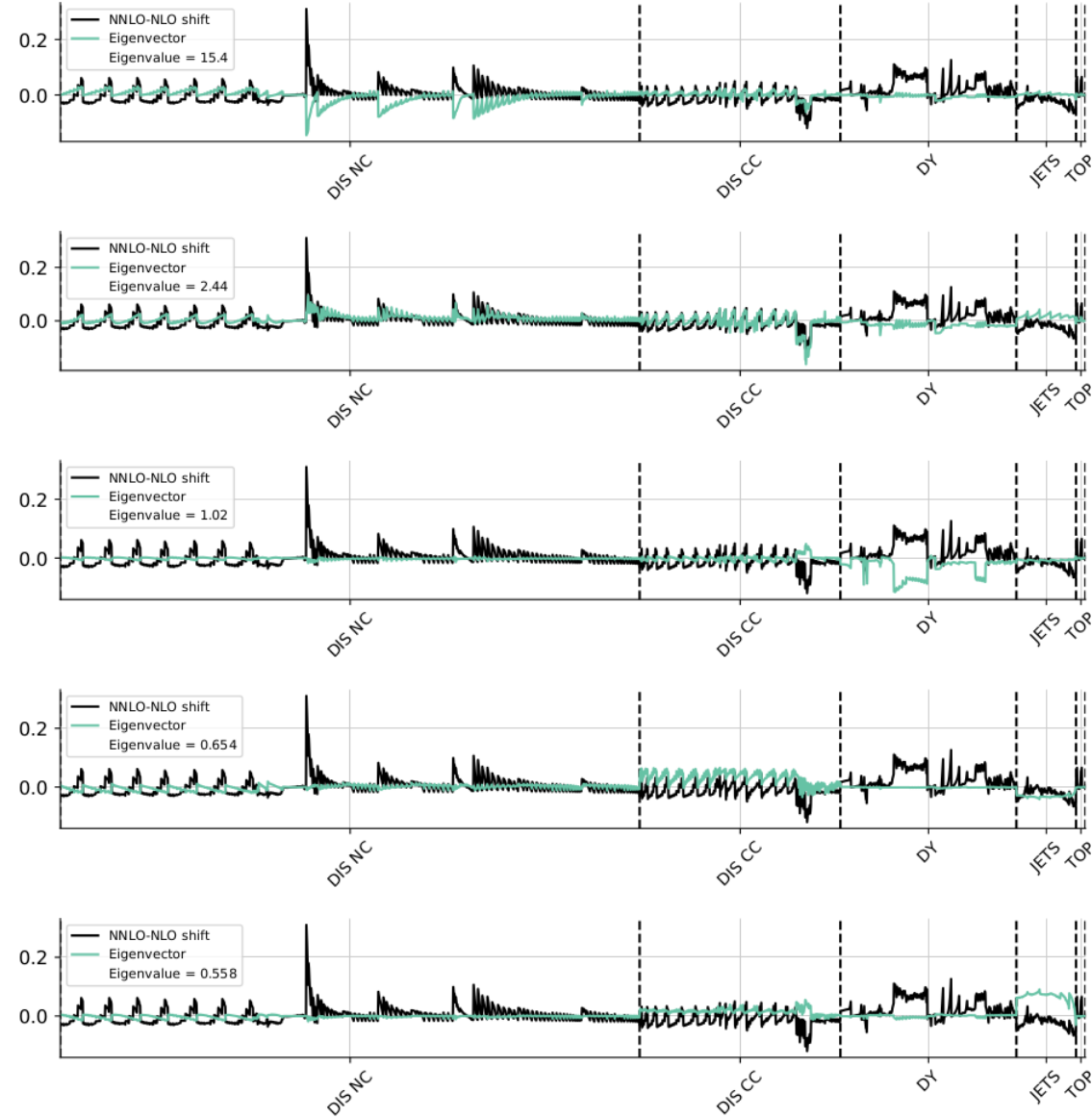
Inspection of these plots confirms that all the prescriptions seem to perform reasonably well. The largest eigenvalue is always very similar in size to the shift, and the size of the eigenvalues generally falls as the projected shifts get smaller. As expected, the 3-point prescription clearly overestimates uncertainties, since $\delta^{\alpha}<s^{\alpha}$ for all the eigenvalues. The same is true, but to a lesser extent, for both 5-point and $\overline{5}$ -point. For the more complicated 7-point and 9-point prescriptions the largest projections (corresponding to the first seven or eight eigenvalues) are estimated rather well, though still perhaps a little conservatively, but for the smaller projections the scatter increases significantly, with some projected shifts hardly predicted at all. This is perhaps not surprising: when varying just six independent scales, we can only expect to obtain only a limited amount of information on the MHO terms. However the correct estimation of the largest projected shifts shows that the theory covariance matrix is giving a reasonable estimation of the MHOU, especially when implemented through the more complicated prescriptions.

On each of these plots, we also show the length of the component $\delta^{\rm miss}_{i}$ that is orthogonal to $S$ , and thus completely outside $E$ . For the symmetric prescriptions, $|\delta^{\rm miss}_{i}|$ is always less than the largest component of $\delta$ in $S$ , while for the asymmetric prescriptions it is greater, very significantly so for the 3-point prescription. This is another indication that the symmetric prescriptions give a better account of the correlations in theoretical uncertainties.

A more detailed understanding of the physical meaning of each eigenvector can be acquired by inspecting its components $e_{i}^{\alpha}$ in the data space. These are shown in Fig. 5.10 for the eigenvectors corresponding to the five largest eigenvalues in the 9-point prescription: the shift vector $\delta_{i}$ is also shown for comparison. It is clear that there is a close correspondence between eigenvectors and MHO contributions to individual processes. For instance the first eigenvector contributes mostly to DIS NC, the second to both DIS NC and DIS CC, the third to DY, the fourth mainly to DIS CC, and the fifth mainly to JETS. Clearly the ordering of these larger eigenvalues is related to the number of data points for the respective processes: the more datapoints, the larger the eigenvalue of the (correlated) uncertainty estimate. Even relatively small eigenvalues can give an important contribution, though to processes with fewer datapoints: for example the ninth eigenvector (not shown) clearly dominates TOP.

In summary, from these validation tests it is apparent that the 9-point prescription gives a reasonable estimate of most of the MHOU, both for individual processes and for the global dataset, with the 7-point being just slightly worse. Based on this, we will therefore adopt 9-point as a default prescription for the theory covariance matrix in the PDF determination to be discussed in the next section.

6 PDFs with missing higher order uncertainties

We can now present the main results of this work: the first determination of the parton distributions of the proton which systematically accounts for the MHOUs affecting the theory calculations of the input processes for the fit. First we present the results for PDFs obtained by fitting only DIS data. This provides us with an initial test case, which we will study by comparing PDFs obtained including the combined experimental and theoretical covariance matrix to the corresponding baseline fit in which only experimental uncertainties are included.

We then turn to the global PDF determination, which offers a nontrivial validation of our methodology, specifically by comparing NLO PDFs, with and without MHOUs, to NNLO PDFs. For global fits, we also study the stability of the results to changes in the prescription used for the computation of the theory covariance matrix: specifically, we compare PDFs obtained with the 9-point prescription (which is our default) to those based on the 7- and 3-point ones. We also study PDFs determined by only partially including the theory covariance matrix, either only in the data generation or only in the fitting. As discussed in the introduction, this provides us with a way of disentangling the impact of the theory covariance matrix on the central value of the PDFs or on the PDF uncertainty.

As discussed in Sect. 2, the theory uncertainties are included by simply replacing the experimental covariance matrix $C_{ij}$ with the sum $(C+S)_{ij}$ of the experimental and theory covariance matrices in the expression for the likelihood of the true value given the data. The NNPDF methodology, as used specifically in the determination of the most recent NNPDF3.1 PDF set [5], is otherwise unchanged. Within this methodology, the covariance matrix is used to generate $N_{\rm rep}$ pseudodata replicas $D^{(k)}_{i}$ for each datapoint $i$ , with $k=1,\dots,N_{\rm rep}$ , whose distribution must reproduce the covariance of any two data points. This means that with theory uncertainties included,

\lim_{N_{\rm rep}\to\infty}{{1}\over{N_{\rm rep}(N_{\rm rep}-1)}}\sum_{k=1}^{N_{\rm rep}}\left(D_{i}^{(k)}-\langle D_{i}\rangle\right)\left(D_{j}^{(k)}-\langle D_{j}\rangle\right)=C_{ij}+S_{ij},

(6.1)

with $\langle D_{i}\rangle={{1}\over{N_{\rm rep}}}\sum_{k=1}^{N_{\rm rep}}D_{i}^{(k)}$ denoting the average over Monte Carlo replicas.

A PDF replica is then fitted to each pseudodata replica $D_{i}^{(k)}$ by minimizing a figure of merit, which in the presence of theory uncertainties becomes

\chi^{2}={{1}\over{N_{\rm dat}}}\sum_{i,j=1}^{N_{\rm dat}}\left(D_{i}-T_{i}\right)\left(C+S\right)^{-1}_{ij}\left(D_{j}-T_{j}\right),

(6.2)

where $T_{i}$ is the theory prediction evaluated with the central scale choice, and the theory covariance matrix $S_{ij}$ is computed using one of the prescriptions presented in Sect. 4.

It is thus clear that the inclusion of a theory-induced contribution in the covariance matrix affects only two steps of the procedure: the pseudodata generation, and the minimization. Everything else is unchanged, and is identical to the default NNPDF methodology. Note that in particular the experimental covariance matrix $C$ used in the fitting is determined, as in NNPDF3.1 and previous NNPDF releases using the so-called $t_{0}$ method for the treatment of multiplicative uncertainties, in order to avoid d’Agostini bias (see Refs. [80, 27] for a detailed discussion). As in previous NNPDF releases, minimization is thus performed using the $t_{0}$ definition of the $\chi^{2}$ , but all $\chi^{2}$ values shown are computed using the covariance matrix as published by the respective experiments.

In the sequel, in order to assess fit quality we will provide $\chi^{2}$ values, and also, we will study the estimator, defined in Ref. [4]

\phi=\sqrt{\langle\chi_{\rm exp}^{2}[T_{i}]\rangle-\chi^{2}_{\rm exp}[\langle T_{i}\rangle]}\,,

(6.3)

where by $\chi_{\rm exp}^{2}[T_{i}]$ we denote the value of the $\chi^{2}$ computed using the $i$ -th PDF replica, and only including the experimental covariance matrix (thus Eq. (6.2), but with $S_{ij}$ set to zero). The average $\chi^{2}$ values which enter Eq. (6.3) are then $\langle\chi^{2}[T_{i}]\rangle$ , the mean value of this $\chi^{2}$ averaged over replicas, and $\chi^{2}[\langle T_{i}\rangle]$ , the value of the $\chi^{2}$ computed using the “central” PDF set which is found by averaging over replicas.

It was shown in Ref.[4] that $\phi$ then gives the average over all datapoints of the ratio of the uncertainties of the predictions to the uncertainties of the original experimental data, taking account of correlations:

\phi=\Big({{1}\over{N_{\rm dat}}}\sum_{i,j=1}^{N_{\rm dat}}(C)^{-1}_{ij}T_{ij}\Big)^{1/2}\,,

(6.4)

where $T_{ij}=\langle T_{i}T_{j}\rangle-\langle T_{i}\rangle\langle T_{j}\rangle$ is the covariance matrix of the theoretical predictions. For an uncorrelated covariance matrix, this is just the ratio of the uncertainty in the prediction using the output PDF to that of the original data. Hence, the value of $\phi$ provides an estimate of the mutual theoretical consistency of the data which are being fitted: consistent data are combined by the underlying theory and lead to an uncertainty in the prediction which is significantly smaller than that of the original data. Note that $\phi$ is always defined so that the uncertainty in the prediction is normalized to the original experimental uncertainty (rather than combined experimental and theory uncertainties). In particular, when considering PDFs determined including a theory covariance matrix, this means that PDFs are determined minimizing the $\chi^{2}$ Eq. (6.2), but $\chi^{2}_{\rm exp}$ is instead used in the computation of $\phi$ Eq. (6.3).

When changing the covariance matrix from $C$ to $C^{\prime}=C+S$ the fluctuations of the replicas will change, according to Eq. (6.1), and if theoretical uncertainties change in the same proportion one would expect the value of $\phi$ to become $\phi^{\prime}=r_{\phi}\phi$ , with

r_{\phi}=\Big(1+{{1}\over{N_{\rm dat}}}\sum_{i,j=1}^{N_{\rm dat}}(C)^{-1}_{ij}S_{ij}\Big)^{1/2}.

(6.5)

Thus, when including MHOU, all else being equal, we would expect PDF uncertainties to increase by a factor $r_{\phi}$ . This will provide us with a baseline to which we can compare the change in uncertainty which is actually observed.

All the PDF sets which have been produced and which will be discussed in this section are listed in Table 6.1. For each of the fits, we indicate its label, the input dataset, the perturbative order and the covariance matrix used. For the fits that include a theory covariance matrix, we also indicate the prescription with which it has been constructed. In the remainder of this section we discuss the main features of these PDF sets.

Label	Dataset	Order	Cov. Mat.	Comments
NNPDF31_nlo_as_0118_dis_kF_1_kR_1	DIS	NLO	$C$	baseline DIS-only NLO
NNPDF31_nlo_as_0118_dis_scalecov_9pt	DIS	NLO	$C+S^{(\rm 9pt)}$
NNPDF31_nnlo_as_0118_dis_kF_1_kR_1	DIS	NNLO	$C$	baseline DIS-only NNLO
NNPDF31_nlo_as_0118_kF_1_kR_1	Global	NLO	$C$	baseline Global NLO
NNPDF31_nlo_as_0118_scalecov_9pt	Global	NLO	$C+S^{(\rm 9pt)}$
NNPDF31_nlo_as_0118_scalecov_7pt	Global	NLO	$C+S^{(\rm 7pt)}$
NNPDF31_nlo_as_0118_scalecov_3pt	Global	NLO	$C+S^{(\rm 3pt)}$
NNPDF31_nlo_as_0118_scalecov_9pt_fit	Global	NLO	$C+S^{(\rm 9pt)}$	$S$ only in $\chi^{2}$ definition
NNPDF31_nlo_as_0118_scalecov_9pt_sampl	Global	NLO	$C+S^{(\rm 9pt)}$	$S$ only in sampling
NNPDF31_nnlo_as_0118_kF_1_kR_1	Global	NNLO	$C$	baseline Global NNLO

Table 6.1: Summary of the PDF sets discussed in this section. The dataset, perturbative order and nature of the treatment of uncertainties for each set are indicated.

6.1 DIS-only PDFs

We first discuss PDF sets based on DIS data only. Fit quality indicators are collected in Table 6.2. The theory covariance matrix is always constructed using the 9-point prescription. We show the value of $\chi^{2}/N_{\rm dat}$ and of the $\phi$ estimator defined in Eqs. (6.2,6.3) respectively. Results are shown for both the total dataset and for the individual DIS experiments of Table 5.1. Note that the total $\chi^{2}$ is no longer just the weighted sum of the individual $\chi^{2}$ s, because it now also includes correlations between experiments.

NNPDF3.1 DIS-only fits
		$\chi^{2}/N_{\rm dat}$			$\phi$
Dataset	$n_{\rm dat}$	NLO		NNLO	NLO		NNLO
		$C$	$C+S^{(\rm 9pt)}$	$C$	$C$	$C+S^{(\rm 9pt)}$	$C$
NMC	134	1.259	1.236	1.239	0.388	0.464	0.444
SLAC	12	0.908	0.543	0.791	0.247	0.590	0.343
BCDMS	530	1.046	1.017	1.047	0.339	0.505	0.389
CHORUS	430	0.982	0.856	1.124	0.409	0.418	0.512
NuTeV	41	0.628	0.491	0.872	0.940	0.994	1.35
HERA incl	967	1.097	1.066	1.104	0.280	1.013	0.335
HERA $F_{2}^{c}$	31	1.047	0.997	1.033	0.526	1.097	0.631
Total	2145	1.061	1.032	1.095	0.358	0.780	0.441

Table 6.2: The values of the

\chi^{2}/N_{\rm dat}

and of the

\phi

estimator in the NNPDF3.1 DIS-only fits with the theory covariance matrix

S^{\rm(9pt)}

, compared to the results based on including only the experimental covariance matrix

C

It is apparent from Table 6.2 that in all cases the $\chi^{2}$ improves when including the theory covariance matrix, both for individual experiments and for the total dataset. Specifically, the $\chi^{2}$ decreases by about 2-3% when including theory a covariance matrix $S^{\rm(9pt)}$ evaluated with the 9-point prescription.

The value of $\phi$ increases very substantially, suggesting a significant increase in the PDF uncertainty. The expected increase according to Eq. (6.5) is $r_{\phi}=2.07$ : NLO MHOUs in DIS are much larger than experimental uncertainties. The observed increase, by a factor of $2.17$ , is in good agreement with this expectation. It is interesting to observe that the NNLO value of $\phi$ is actually also rather larger than the NLO value, though not quite so much larger, suggesting that at NNLO the MHOUs in DIS might still be quite large.

Next we compare PDFs: in Fig. 6.1 we compare the gluon and the total quark singlet PDF at $Q=10$ GeV with and without MHOUs in the covariance matrix, determined using the 9-point prescription. The NLO results are also compared with the central value of the NNLO fit based on the experimental covariance matrix only. Note that in these comparison plots the PDF uncertainty band is always computed using standard NNPDF methodology, i.e., as the standard deviation over the PDF replica sample. Therefore, this uncertainty band has a different meaning dependent on whether or not the theory covariance matrix is included: when it is not included, the band represents the conventional “PDF uncertainty”, reflecting the uncertainties from the data (and methodology), while when it is included, the band provides the combined “PDF” and MHO uncertainty.

Figure 6.1: Comparison of DIS-only PDFs determined with and without MHOUs in the covariance matrix. The gluon (left) and quark singlet (right) are shown at

Q=10

GeV. The theory covariance matrix

S

has been constructed using the 9-point prescription. The central value of the NNLO determined without MHOU is also shown. All results are shown as a ratio to the central value of the set with theory covariance matrix not included. Note that the uncertainty band has a different meaning according to whether the theory covariance matrix is included or not: if not it is the standard PDF uncertainty coming from data, while if it is included, then it is the total uncertainty including the MHOU.

The comparison shows that for PDFs which are strongly constrained by data, such as the quark singlet PDF for $x\mathrel{\hbox to0.0pt{\lower 4.0pt\hbox{\hskip 1.0pt$\sim$}\hss}\raise 1.0pt\hbox{$>$}}10^{-3}$ , the uncertainty does not increase much upon inclusion of the theory covariance matrix, and sometimes it even decreases. However, for several PDFs, including the gluon PDF, which is only loosely constrained by the DIS data, the uncertainty increases substantially with MHOUs. This is of course consistent with the fact that, in the absence of stringent experimental constraints, an extra contribution to the covariance matrix will lead to increased uncertainties in the best fit.

6.2 Global PDFs

We now discuss PDFs determined from the global dataset presented in Sect. 5.1. Only NLO PDFs will be discussed here, with global NNLO PDFs left for future work. The $\chi^{2}$ values and $\phi$ values are shown in Tables 6.3 and 6.4 respectively, both for the total dataset and for the individual processes of Table 5.1. In comparison to the DIS-only case of Table 6.2 we now also show results obtained using the 7-point and 3-point prescriptions, and also for the default 9-point prescription but where the results were obtained by including the theory covariance matrix either only in the $\chi^{2}$ definition Eq. (6.2), or only in the data generation Eq. (6.1), in order to understand better the two distinct effects. The baseline NLO and NNLO PDF sets (without theory covariance matrix) are identical in all respects to the NNPDF3.1 PDF sets [68], except for the somewhat different dataset as discussed in Sect. 5.1.

As in the case of the DIS-only fit, upon adding the MHOU we find a reduction of $\chi^{2}$ both for the global fit and for individual datasets. Specifically, the $\chi^{2}$ for the NLO global fit with theory covariance matrix computed with the 9-point prescription decreases by about 3%, and almost coincides with the NNLO $\chi^{2}$ , suggesting that indeed the theory uncertainty is correctly accounting for the missing NNLO correction. The pattern at the level of individual datasets is more complex, due to a variety of reasons. In particular, consider the CMS $Z$ $p_{T}$ distribution, where a very significant decrease in $\chi^{2}$ is observed when going from NLO to NNLO, but not when adding the theory uncertainty to the NLO. This turns out to be due to a sizable uncorrelated uncertainty which must be added to the NNLO theory prediction in order to account for numerical instabilities (see the discussion of Fig. 6 in Ref. [68]).

On the other hand, the value of $\phi$ now increases much less than expected: with our favorite 9-point prescription the increase is by about 30%, while the expected $r_{\phi}=1.69$ . This is an indication that by accounting for the missing NNLO terms, the inclusion of MHOUs resolves some of the tensions in the fit with only the experimental uncertainties, thus reducing the overall effect of the MHOUs. The NNLO fit also shows an increase, to $0.36$ , but the fact that this is already quite close to $0.41$ perhaps suggests that the effect of adding MHOUs to the NNLO global fit will be relatively modest.

Comparing the different prescriptions, results are reasonably stable, even when comparing to the 3-point prescription which, as discussed in Sects. 4.3-5.3, spans a much smaller subspace of theory variations. However, the 9-point prescription appears to perform best in terms of $\chi^{2}$ quality with very little difference in $\phi$ , in agreement with the results of Sect. 5.4.

We finally turn to fits in which the theory covariance matrix is included either in the $\chi^{2}$ definition Eq. (6.2) but not in the data generation Eq. (6.1), or in the data generation Eq. (6.1) but not in the $\chi^{2}$ definition Eq. (6.2). In the former case, we expect the MHOUs to affect mostly the central value (since the relative weighting of different data points is altered during the fitting according to the relative size of their MHOUs), and to a lesser extent the uncertainties (since the data replicas only fluctuate according to the experimental uncertainties). The results show that indeed including the MHOU in the $\chi^{2}$ definition alone leads to a $\chi^{2}$ value which is very close to that found when the MHOU is fully included, consistent with the expectation that it is the inclusion of the theory covariance matrix in the $\chi^{2}$ which mostly drives the best fit, while the $\phi$ value increases somewhat less. In the latter case, we expect to obtain increased uncertainties but a worse fit, since the data replica fluctuations are wider due to the MHOU, and this is not accounted for in the $\chi^{2}$ . The results indeed show a significant deterioration of fit quality, as expected for an inconsistent fit: the $\chi^{2}$ goes up, and also the $\phi$ value goes up dramatically, showing the increase in uncertainty due to the inclusion of MHOU in the sampling, now uncompensated by a rebalancing of the datasets through the inclusion of MHOU in the fit.

		$\chi^{2}/N_{\rm dat}$ in the NNPDF3.1 global fits
Dataset	$n_{\rm dat}$	NLO						NNLO
		$C$	$C+S^{(\rm 9pt)}$	$C+S^{(\rm 7pt)}$	$C+S^{(\rm 3pt)}$	$C+S^{(\rm 9pt)}_{\rm fit}$	$C+S^{(\rm 9pt)}_{\rm samp}$	$C$
NMC	134	1.241	1.239	1.264	1.253	1.235	1.246	1.222
SLAC	12	0.868	0.503	0.485	0.509	0.493	0.738	0.693
BCDMS	530	1.040	1.029	1.046	1.062	1.033	1.042	1.062
HERA $\sigma_{\rm NC}^{p}$	886	1.086	1.044	1.046	1.079	1.044	1.190	1.098
HERA $\sigma_{\rm NC}^{c}$	31	1.395	1.037	1.082	1.172	1.055	1.563	1.163
DIS NC	1593	1.088	1.079	1.086	1.095	1.081	1.227	1.084
NuTeV dimuon	41	0.474	0.388	0.355	0.359	0.421	0.406	0.470
CHORUS	430	1.037	0.891	0.896	0.900	0.898	1.081	1.124
HERA $\sigma_{\rm CC}^{p}$	81	1.154	1.070	1.067	1.106	1.062	1.103	1.126
DIS CC	552	1.012	0.928	0.933	0.960	0.929	1.036	1.079
ATLAS $W,Z$ 7 TeV 2010	30	0.999	0.880	0.916	0.975	0.892	0.984	0.935
ATLAS $W,Z$ 7 TeV 2011	34	3.306	2.224	2.282	2.389	2.205	3.107	1.807
ATLAS low-mass DY 7 TeV	4	0.684	0.654	0.668	0.690	0.660	0.733	1.024
ATLAS high-mass DY 7 TeV	5	1.677	1.736	1.700	1.660	1.667	1.577	1.498
ATLAS $Z$ $p_{T}$ 8 TeV ( $p_{T}^{ll},M_{ll}$ )	44	1.171	1.067	1.070	1.067	1.062	1.183	0.907
ATLAS $Z$ $p_{T}$ 8 TeV ( $p_{T}^{ll},y_{ll}$ )	48	1.666	1.583	1.614	1.688	1.638	1.641	0.865
CMS Drell-Yan 2D 2011	88	1.220	1.067	1.098	1.169	1.062	1.132	1.319
CMS W asy 840 pb	11	0.965	1.022	0.966	0.987	1.045	1.034	0.863
CMS W asy 4.7 fb	11	1.662	1.670	1.704	1.713	1.659	1.657	1.750
CMS W rap 8 TeV	22	0.955	0.611	0.609	0.587	0.627	0.665	0.826
CMS $Z$ $p_{T}$ 8 TeV ( $p_{T}^{ll},M_{ll}$ )	28	3.895	3.745	3.712	3.836	3.706	3.905	1.339
LHCb $Z$ 940 pb	9	1.238	1.191	1.162	1.179	1.165	1.281	1.437
LHCb $Z\to ee$ 2 fb	17	1.305	1.303	1.305	1.313	1.334	1.250	1.203
LHCb $W,Z\to\mu$ 7 TeV	29	1.262	1.106	1.267	1.261	1.134	1.207	1.536
LHCb $W,Z\to\mu$ 8 TeV	30	1.194	1.027	1.125	1.154	1.054	1.152	1.438
CDF $Z$ rap	29	1.554	1.313	1.433	1.505	1.311	1.418	1.510
D0 $Z$ rap	28	0.649	0.601	0.626	0.640	0.597	0.618	0.604
D0 $W\to e\nu$ asy	8	1.176	1.066	1.055	1.083	1.029	1.200	2.558
D0 $W\to\mu\nu$ asy	9	1.400	1.450	1.372	1.361	1.439	1.395	1.374
DY	484	1.486	1.447	1.485	1.483	1.461	1.434	1.231
ATLAS jets 2011 7 TeV	31	1.069	1.019	1.065	1.079	1.026	1.031	1.076
CMS jets 7 TeV 2011	133	0.869	0.786	0.790	0.830	0.795	0.883	0.921
JETS	164	0.907	0.839	0.858	0.901	0.848	0.911	0.950
ATLAS $\sigma_{tt}^{\rm top}$	3	2.577	0.787	0.853	0.982	0.770	2.442	0.903
ATLAS $t\bar{t}$ rap	10	1.258	0.955	0.867	0.910	0.935	1.355	1.424
CMS $\sigma_{tt}^{\rm top}$	3	0.984	0.170	0.234	0.333	0.158	0.859	0.140
CMS $t\bar{t}$ rap	10	0.950	0.910	0.923	0.933	0.916	0.942	1.039
TOP	26	1.260	1.012	1.016	1.077	1.001	1.264	1.068
Total	2819	1.139	1.109	1.129	1.139	1.113	1.220	1.105

Table 6.3: The values of the

\chi^{2}/N_{\rm dat}

in NLO global fits with the theory covariance matrix

S

, compared to the results based on including only the experimental covariance matrix

C

. Results are shown for the 9-, 7-, and 3- point prescriptions. For the 9-point prescription we also show results obtained including the theory covariance matrix in the

\chi^{2}

definition Eq. (6.2) but not in the data generation Eq. (6.1) (marked

S_{\rm fit}^{9pt}

) and then in the data generation Eq. (6.1) but not in the

\chi^{2}

definition Eq. (6.2) (marked

S_{\rm sampl}^{9pt}

). Values corresponding to the NNLO fit with experimental covariance matrix

C

only are also shown.

	$\phi$ in the NNPDF3.1 global fits
Process	NLO						NNLO
	$C$	$C+S^{(\rm 9pt)}$	$C+S^{(\rm 7pt)}$	$C+S^{(\rm 3pt)}$	$C+S^{(\rm 9pt)}_{\rm fit}$	$C+S^{(\rm 9pt)}_{\rm sampl}$	$C$
DIS NC	0.266	0.412	0.393	0.384	0.414	1.137	0.305
DIS CC	0.389	0.408	0.427	0.442	0.388	0.502	0.471
DY	0.361	0.377	0.369	0.379	0.378	0.603	0.380
JETS	0.295	0.359	0.327	0.333	0.336	0.461	0.392
TOP	0.375	0.443	0.387	0.405	0.382	0.612	0.363
Total	0.314	0.405	0.394	0.394	0.400	0.932	0.362

Table 6.4: Same as Table 6.3, but for the values of the

\phi

estimator.

We now move on to discuss the corresponding results at the PDF level, in analogy with the comparisons presented for the DIS-only fits in Fig. 6.1. Specifically, in Fig. 6.2. we show the results of the NLO fits based on $C$ and $C+S^{\rm(9pt)}$ , as well as the central value of the NNLO fit based on $C$ , for the gluon, the total quark singlet, the anti-down quark, and the total strangeness PDFs, all at $Q=10$ GeV. We also show in Fig. 6.2 the same PDFs but at the scale $Q=1.6$ GeV at which PDFs are parametrized.

Figure 6.2: Same as Fig. 6.1 now for the NNPDF3.1 global fits. We show the results of the NLO fits based on

C

and

C+S^{\rm(9pt)}

normalized to the former, as well as the central value of the NNLO fit based on

C

. for the gluon, the total quark singlet, the anti-down quark, and the total strangeness PDFs, all at

Q=10

GeV.

We find that in the data region the PDF uncertainty is only very moderately increased by the inclusion of the theory covariance matrix, while central values can shift significantly, by up to one sigma. This is consistent with the observation that the $\phi$ values in Table 6.4 increase by only a moderate amount upon inclusion of the theory covariance matrix. This provides evidence that in the data region the inclusion of the theory covariance matrix resolves tensions which are otherwise present in the global dataset. In contrast, in regions where PDFs which are only loosely constrained by the data, and in particular in the extrapolation regions, the PDF uncertainty increases significantly.

Figure 6.3: Same as Fig. 6.2 but now with results shown at the scale

Q=1.6

GeV at which PDFs are parametrized.

When comparing PDFs at the parametrization scale in Fig. 6.3, an especially interesting comparison is with respect to the central NNLO value: not only is this quite compatible with the uncertainty band, but there is now clear evidence that upon inclusion of the NLO MHOU the central best fit moves towards the correct NNLO result. Of course, this improved agreement of the best-fit NLO and NNLO PDFs is scale-dependent, since PDFs at NLO and NNLO evolve in different ways, and the scale at which NLO and NNLO become closest will depend on the scale of the data which dominate the determination of each PDF combination. However, the agreement is seen in Fig. 6.2 to persist by and large also at high scale. This is further evidence that indeed the theory covariance matrix has resolved tensions due to MHOs. This improved agreement of the central value of the NLO $C+S^{(\rm 9pt)}$ with the NNLO $C$ fits is non-trivial: for instance, inclusion of the theory covariance matrix leads to a suppression of the gluon at large $x$ and an enhancement of strangeness, both of which are indeed also observed at NNLO.

Next, in Fig. 6.4 we compare PDFs obtained using different prescriptions. The corresponding relative PDF uncertainties are compared in Fig. 6.5. In agreement with what we saw for the $\chi^{2}$ and $\phi$ values in Tables 6.3, 6.4 results are quite stable with respect to the choice of prescription, though in the most extreme case of the 3-point prescription, where factorization scale variations are entirely uncorrelated between different processes, we observe somewhat smaller uncertainties, and a central value which is closer to that when the MHOU is not included.

Figure 6.4: Same as Fig. 6.2 now comparing the results of the NNPDF3.1 global fits with the theory covariance matrix constructed accordingly to the 3-, 7-, and 9-point prescriptions, normalized to the central value of the latter.

Figure 6.5: Same as Fig. 6.4, now showing relative PDF uncertainties, normalized to the central value of the baseline set. Note that the

y

-axes ranges are different for each PDF combination.

Finally, in Fig. 6.6 we compare PDFs obtained including the theory covariance matrix only in the $\chi^{2}$ definition Eq. (6.2) but not in the data generation Eq. (6.1) and conversely. We see that when the theory covariance matrix is included in the replica generation but not in the $\chi^{2}$ , uncertainties increase very significantly. This result is in agreement with the observation from Table 6.3 that in this case the fit quality significantly deteriorates, which is because the fit becomes inconsistent due to the $\chi^{2}$ not matching the wider fluctuations in the data. The effect is particularly visible for the quark distributions. On the other hand, including the theory covariance matrix only in the $\chi^{2}$ singles out the effect of the theory covariance matrix on central values, due to rebalancing of datapoints in the fit according to their relative MHOU. Indeed in this case the central value is very close to that obtained when including the MHOU is both data generation and fit. We also see that the change in uncertainties in the data region is now very small, consistent with Table 6.3. These results confirm our expectation that in the full fit, while the MHOU results in a substantial increase in the fluctuations of data replicas, this is compensated by a relaxation of tensions due to the inclusion of MHOU the fit, with the net result that while central values shift, overall uncertainties do not increase much.

Figure 6.6: Same as Fig. 6.2, now comparing the results of the baseline

C+S^{(\rm 9pt)}

fit with those in which the theory covariance matrix

S

is included either in the

\chi^{2}

definition or in the generation of Monte Carlo replicas, but not on both.

7 Implications for phenomenology

Whereas a full assessment of the impact of the inclusion of MHOU in PDFs will be possible only once we have global NNLO sets with MHOU, it is worth performing a first phenomenological investigation, by computing reference LHC standard candles with the NLO PDF sets which include MHOUs presented in Sect. 6, and comparing to results with the corresponding NLO PDF sets in which no MHOU is included.

In this section we will specifically consider Higgs boson production in gluon-fusion and in vector-boson fusion, top quark pair and $Z$ and $W$ electroweak gauge boson production. Note that the latter processes are among those which have been used for PDF determination, see Tab. 5.1. This raises the issue of possible double counting of uncertainties between the MHOU in the PDF and in the hard matrix element. This will be addressed in Sect. 8.1 below.

As discussed in Sect. 6, once the MHOU is included in the covariance matrix, the standard NNPDF methodology can be used, but with the PDF uncertainties now also including a theory-induced contribution. Specifically, PDF uncertainties (which now include the MHOU uncertainty) are obtained as standard deviations over the replica sample. The total uncertainty on a physical prediction is then obtained by combining this uncertainty with that on the hard cross-section for the given process. The latter is conventionally obtained as the envelope of a 7-point scale variation, see e.g. Ref. [18]. Of course, an alternative possibility is to compute the theory uncertainty on the hard cross-sections in exactly the same way as we compute it when performing PDF determination, i.e. using the theory covariance matrix. In this case, the MHOU on any measurement is found as the diagonal element of the covariance matrix, evaluated for the given measurement. Here we will compute the theory uncertainty both using the theory covariance matrix (with the 9-point prescription, given in Eq. (4.9)), and as a 7-point envelope. The MHOU uncertainty on the hard cross-section can then be combined with the total uncertainty on the PDF (which includes both MHOU and data uncertainties) in quadrature. A more detailed discussion of prescriptions for the computation of the total uncertainty on a physical observable, including explicit formulae, will be given in Sect. 8.1 below.

The current state of the art for precision phenomenology is NNLO, and thus NNLO PDFs would be needed for accurate predictions. However, as discussed in Sect. 6, at present only NLO global PDFs with MHOU are available. In principle, NNLO PDFs from a DIS only fit are also available. However, also as discussed in Sect. 6, some of these PDFs (specifically the gluon) are affected by large uncertainties due to the lack of experimental constraints. The comparison of PDFs with and without MHOU for such sets would thus be rather misleading. Therefore, in this section we will focus on NLO PDFs. It should of course be kept in mind that NNLO PDFs with MHOU are likely to have smaller uncertainties.

7.1 Higgs production

We first discuss Higgs production in gluon fusion (ggF) and in vector boson fusion (VBF). These two processes are of direct relevance for the characterization of the Higgs sector and are both currently known at N³LO accuracy [81, 82, 83, 84]. Note that the perturbative behavior and leading partonic channels for these processes are quite different. Higgs production in gluon fusion is driven by the gluon-gluon luminosity and its perturbative expansion converges slowly, with manifest convergence reached only at N³LO. Vector boson fusion is driven by the quark-antiquark luminosity and it exhibits fast perturbative convergence.

In Table 7.1 we present predictions for Higgs production in gluon fusion at the LHC for $\sqrt{s}=13$ TeV. We perform the calculation at NLO, NNLO and N³LO in the rescaled effective theory approximation using ggHiggs [85, 86, 87, 88, 89, 90] with $\mu_{f}=\mu_{r}=m_{H}/2$ as central scale, with the NLO global sets obtained in this paper, with and without MHOUs, as input PDFs at all orders. The results are displayed graphically in Fig. 7.1, where, for the NNLO computation, we also show the central value found using NNLO PDFs.

We find that for all perturbative orders the central values obtained with PDFs with and without MHOU are very similar, while the PDF uncertainty is about 50% larger when MHOU are included in the PDF fit. This can be understood by noticing that for the intermediate values of the momentum fraction, $x\simeq 10^{-2}$ , relevant for Higgs production in gluon fusion, the PDF uncertainty of the gluon is increased in the $C+S^{(\rm 9pt)}$ fit as compared to the $C$ -only fits, see Fig. 6.2. Comparison to the result obtained using NNLO PDFs (for the NNLO computation) shows that upon inclusion of the MHOU the PDF uncertainty band of the result with NLO PDFs now includes the NNLO PDF result, while it would not in the absence of MHOU, both because of the (small) shift in central value and of the widening of the uncertainty band.

From Table 7.1 one can also observe that the MHOU on the hard matrix element uncertainty $\sigma_{\mathcal{F}}^{\rm th}$ evaluated using the 9-point theory covariance matrix, Eq. (4.9), is compatible with the canonical 7-point envelope if the latter is symmetrized by taking the maximum value between the lower and upper uncertainties. In particular, the theory covariance matrix estimate is slightly larger than the envelope prescription at NLO and at NNLO, while it becomes a little smaller at N³LO. Even so, the NLO uncertainty band does not contain the NNLO central value, which lies just above the edge of the band.

Higgs production in gluon fusion at 13 TeV
	$C$	$C+S^{(\rm 9pt)}$
NLO	37.63 $\pm$ 1.14% $\pm$ 24.67 (22.69) %	37.45 $\pm$ 1.69% $\pm$ 24.67 (22.69) %
NNLO	47.38 $\pm$ 1.12% $\pm$ 11.82 (10.09) %	47.16 $\pm$ 1.65% $\pm$ 11.83 (10.09) %
N³LO	49.04 $\pm$ 1.12% $\pm$ 3.35 (3.85) %	48.81 $\pm$ 1.65% $\pm$ 3.35 (3.85) %

Table 7.1: The total cross-sections for Higgs production in gluon fusion (in pb) obtained by using NLO global PDFs based on either

C

C+S^{{\rm(9pt)}}

, see Table 6.1. We quote the central prediction, the total PDF uncertainty (first) and the MHOU uncertainty on the hard cross-section (second) expressed as a percentage of the central value. The latter is evaluated both using the theory covariance matrix (9-point prescription) or, in parenthesis, a (symmetrized) envelope of the 7-point scale variations (see Sect. 8.1), obtained by taking the maximum value between the lower and upper uncertainties.

Figure 7.1: Graphical representation of the results of Tables 7.1 and 7.2. At each perturbative order the pair of uncertainty bands on the left (blue) is computed with PDFs based on the experimental covariance matrix

C

, while the pair of uncertainty bands on the right (red) with PDFs based on the combined experimental and theoretical covariance matrix

C+S

(9-point prescription). The light-shaded bands represent the uncertainty on the hard cross-section (“scale uncertainty”) evaluated using the theory covariance matrix (see text) the dark bands represent the PDF uncertainty. For the NNLO result, we also show the central value obtained using NNLO PDFs as a dashed horizontal line.

We conclude that using NLO PDFs in the N³LO calculation, the inclusion of MHOU in the PDFs translates into a few per-mille increase of the PDF uncertainty at the cross-section level. In Ref. [82] NNLO PDFs were used with the N³LO calculation in order to provide a state-of-the art result, and a MHOU uncertainty on the NNLO PDF was estimated based on the difference between results obtained using NLO and NNLO PDFs. Once NNLO PDFs with MHOUs determined within our approach are available it will be interesting to compare our results with this estimate.

We now turn to Higgs production in vector boson fusion. We perform the calculation at N³LO accuracy using proVBFH-inclusive [91, 84]. with central factorization and renormalization scales set equal to the squared four-momentum of the vector boson. Results are collected in Table 7.2 and shown in Fig. 7.1. The MHOU corrections to the PDFs are very small, so PDF uncertainties with or without theory covariance matrix are very similar. Also in this case, like for gluon fusion, the uncertainty on the hard matrix element computed with the 9-point theory covariance matrix is similar to the one obtained by symmetrizing the 7-point envelope.

The smallness of the MHOU in the PDF follows from the fact that VBF Higgs production is driven by the quark-antiquark luminosity, which in turn is dominated by the quark PDF in the data region, whose uncertainties, as we have seen in Sect. 6.2, are almost unaffected by the inclusion of MHOU. Comparison to the result obtained using NNLO PDFs (for the NNLO computation) shows that the NNLO PDF result is at the edge of the PDF uncertainty band of the result with NLO PDFs if MHOU are included, while it is off by almost two $\sigma$ if they are not. This is essentially due to the significant shift in central value, in agreement with the observation made in Sect. 6.2, where we noticed that MHOUs have the effect of moving the central value of the PDFs in the data region towards the NNLO result. The shift in the central value of the VBF cross-section due to the MHOU is in fact quite significant: its size is comparable to the MHOU $\sigma_{\mathcal{F}}^{\rm th}$ on the NLO matrix element, and indeed the shift when going from NLO to NNLO matrix elements, and thus much larger that the corresponding N³LO correction.

We conclude that for VBF the main effect of including the MHOU in the PDF is a significant shift in the central value of the prediction. Also in this case estimates of the MHOU on the NNLO PDF were presented in Ref. [84], and it will be interesting to compare them to our approach once NNLO PDFs with MHOU determined within our approach are available.

Higgs production in VBF at 13 TeV
	$C$	$C+S^{(\rm 9pt)}$
NLO	3.966 $\pm$ 1.12% $\pm$ 0.66 (0.66) %	3.995 $\pm$ 1.17% $\pm$ 0.66 (0.65) %
NNLO	3.928 $\pm$ 1.12% $\pm$ 0.37 (0.42) %	3.956 $\pm$ 1.17% $\pm$ 0.37 (0.41) %
N³LO	3.925 $\pm$ 1.12% $\pm$ 0.11 (0.15)	3.953 $\pm$ 1.17% $\pm$ 0.11 (0.14) %

Table 7.2: Same as Table 7.1, now for Higgs production in vector boson fusion.

A common feature of gluon fusion and vector-boson fusion is that it is only upon inclusion of the MHOU that the result found using NNLO PDFs is within or at the edge of the PDF uncertainty band of the result found with NLO PDFs.

7.2 Top quark pair production

We now study the impact of the PDF-related MHOU on the total top-quark pair production cross-section at the LHC for different center-of-mass energies. In Table 7.3 we collect, using the same format as Table 7.1, the predictions for the top-quark pair-production cross-sections at $\sqrt{s}=7$ , 8 and 13 TeV obtained using the top++ code [92] and setting the central scales to $\mu_{f}=\mu_{r}=m_{t}=172.5$ TeV. The results in the case of 8 and 13 TeV are also displayed in Fig. 7.2, where again for at NNLO we also show the result obtained using NNLO PDFs.

$t\bar{t}$ production at 7 TeV
	$C$	$C+S^{(\rm 9pt)}$
NLO	155.42 $\pm$ 1.57% $\pm$ 12.2 (13.0) %	153.94 $\pm$ 2.45% $\pm$ 12.2 (13.0) %
NNLO	174.48 $\pm$ 1.55% $\pm$ 5.52 (6.46) %	172.81 $\pm$ 2.42% $\pm$ 5.52 (6.45) %
$t\bar{t}$ production at 8 TeV
	$C$	$C+S^{(\rm 9pt)}$
NLO	222.45 $\pm$ 1.44% $\pm$ 12.3 (12.8) %	220.42 $\pm$ 2.17% $\pm$ 12.3 (12.8) %
NNLO	249.41 $\pm$ 1.43% $\pm$ 5.43 (6.28) %	247.14 $\pm$ 2.14% $\pm$ 5.43 (6.27) %
$t\bar{t}$ production at 13 TeV
	$C$	$C+S^{(\rm 9pt)}$
NLO	734.21 $\pm$ 1.11% $\pm$ 12.4 (11.8) %	728.57 $\pm$ 1.38% $\pm$ 12.3 (11.8) %
NNLO	819.43 $\pm$ 1.11% $\pm$ 5.16 (5.64) %	813.17 $\pm$ 1.35% $\pm$ 5.16 (5.64) %

Table 7.3: Same as Table 7.1, now for top-quark pair-production at

\sqrt{s}=7,8

and 13 TeV.

Figure 7.2: Same as Fig. 7.1 for top-quark pair production at 8 and 13 TeV, see also Table 7.3.

Just as in the case of Higgs production via gluon-gluon fusion, we find that for top-quark pair production the central values obtained with PDFs with and without MHOU are rather similar, and well within the one- $\sigma$ PDF uncertainty. We also observe that the PDF uncertainty at $\sqrt{s}=7$ and 8 TeV (13 TeV) is about 50% (20%) larger once MHOU are included in the determination of the PDFs. This is again compatible with the corresponding behavior of the gluon PDF shown in Fig. 6.2, where it can be observed that, for $x\simeq 0.1$ , relevant for top pair production at $\sqrt{s}=7$ and 8 TeV, the PDF uncertainty is increased in the $C+S^{\rm(9pt)}$ fit as compared to the $C$ -only fit, while this increase is less marked for $x\sim 0.3$ , relevant for top pair production at $\sqrt{s}=13$ TeV. Also in this case, the NNLO prediction using NLO PDFs is in better agreement with the that using NNLO PDFs once MHOUs are included, and in fact only in this case the latter is within the PDF error band of the former.

In addition, we note once again that the uncertainty on the hard cross-section $\sigma_{\mathcal{F}}^{\rm th}$ evaluated using the 9-point covariance matrix is rather similar to that obtained from the symmetrized 7-point envelope. In particular, the 9-point result is slightly larger (smaller) than the 7-point envelope at NNLO (NLO). Finally, from Fig. 7.2 we notice that for this process the MHOU on the hard cross-section dominates the PDF uncertainty (with or without MHOU included), even with NLO PDFs.

7.3 $Z$ and $W$ gauge boson production

We finally turn to gauge boson production, for which we obtain predictions using the computational framework Matrix [93]. In this formalism, all tree-level and one-loop amplitudes are obtained from OpenLoops [94, 95, 96]. For these theoretical predictions for inclusive $W$ and $Z$ production cross sections at $\sqrt{s}$ = 13 TeV, we adopt realistic kinematic cuts similar to those applied by ATLAS and CMS. The fiducial phase space for the $W^{\pm}$ cross-section is defined by requiring $p_{l,T}\geq 25$ GeV and $\eta_{l}\leq$ 2.5 for the charged lepton transverse momentum and pseudo-rapidity and a missing energy from the neutrino of $p_{\nu,T}\geq 25$ GeV. In the case of $Z$ production, we require $p_{l,T}\geq$ 25 GeV and $|\eta_{l}|\leq$ 2.5 for the charged leptons transverse momentum and rapidity and 66 $\leq m_{ll}\leq$ 116 GeV for the di-lepton invariant mass.

In Table 7.4 we display a similar comparison as in Table 7.1 now for $W$ and $Z$ gauge boson production at $\sqrt{s}=13$ TeV. The corresponding graphical representation of the results is provided in Fig. 7.3, again using the same conventions as in Fig. 7.1 and again also showing the NNLO result with NNLO PDFs.

We find that when including the MHOU the PDF uncertainty is increased by $\simeq 70\%,30\%$ and $75\%$ for $Z$ , $W^{+}$ , and $W^{-}$ production respectively. Given that $W$ and $Z$ production at ATLAS and CMS at $\sqrt{s}=13$ TeV is sensitive to the light sea quarks down to $x\simeq 10^{-3}$ , this increase in the PDF uncertainty once MHOU are accounted for is consistent with the corresponding increase reported in the case of the singlet PDF in Fig. 6.5.

$Z$ production at 13 TeV
	$C$	$C+S^{(\rm 9pt)}$
NLO	0.759 $\pm$ 0.96% $\pm$ 4.18 (4.18) %	0.767 $\pm$ 1.63% $\pm$ 4.16 (4.15) %
NNLO	0.749 $\pm$ 0.97% $\pm$ 0.94 (0.63) %	0.760 $\pm$ 1.64% $\pm$ 0.93 (0.66) %
$W^{-}$ production at 13 TeV
	$C$	$C+S^{(\rm 9pt)}$
NLO	3.534 $\pm$ 0.92% $\pm$ 4.28 (4.34) %	3.560 $\pm$ 1.58% $\pm$ 4.28 (4.34) %
NNLO	3.474 $\pm$ 0.92% $\pm$ 1.03 (0.64) %	3.511 $\pm$ 1.59% $\pm$ 0.99 (0.63) %
$W^{+}$ production at 13 TeV
	$C$	$C+S^{(\rm 9pt)}$
NLO	4.614 $\pm$ 1.00% $\pm$ 4.09 (4.15) %	4.643 $\pm$ 1.73% $\pm$ 4.08 (4.14) %
NNLO	4.582 $\pm$ 0.99% $\pm$ 0.88 (0.58) %	4.631 $\pm$ 1.72% $\pm$ 0.87 (0.62) %

Table 7.4: Same as Table 7.1, now for

W

and

Z

gauge boson production at

\sqrt{s}=13

TeV. The cross-section is given in nb.

Figure 7.3: Same as Fig. 7.1 for

W^{\pm}

and

Z

gauge boson production at

\sqrt{s}=13

TeV, see also Table 7.4.

Similarly to Higgs production in vector-boson-fusion, we find that the inclusion of MHOU in the PDF shifts the central value of the prediction, by an amount which is comparable to or larger than the data-driven PDF uncertainty. Yet again, the agreement of the NNLO prediction with NLO PDFs with that which is obtained when NNLO PDFs are used is significantly improved: for $Z$ production within the PDF error band and for $W$ production just barely outside it. We conclude that for weak gauge boson production at the LHC the impact of the MHOU associated to the PDFs is twofold: on the one hand an overall increase in the PDF uncertainties that ranges between 30% and 70% depending on the process, and on the other hand a shift in the central values which is comparable to that of the PDF uncertainties of the fit without MHOU.

8 Usage and delivery

As mentioned previously, the PDF sets with MHOU presented in Sect. 6 can be used in essentially the same way as the standard NNPDF sets. In this section we discuss how MHOUs included in PDF sets should be combined with those in hard matrix elements, specifically addressing some conceptual issues, and we then provide detailed instructions for their use. We then discuss the delivery of the PDF sets presented in this work, and provide a list of the sets which are being made publicly available by means of the LHAPDF interface.

8.1 Combining MHOUs in PDFs and hard matrix elements

As discussed in the introduction, the MHOU on PDFs discussed in this paper arises due to the fact that PDFs are determined using perturbative computations performed at a finite order in the perturbative expansion, and it manifests itself in the fact that PDFs change when varying the order at which they are determined: NLO and NNLO PDFs differ. We have further seen in Sect. 3 that there exist two distinct sources of MHOU in the PDF: that related to MHOs in the computation of the hard cross-sections for those processes used for PDF determination, and that coming from MHOs in the anomalous dimensions. These two sources of MHOU in the PDFs are respectively associated with renormalization and factorization scale variation and can be treated as independent of each other, at least with the definition given here and summarized in Table 3.1.

On top of this MHOU on the PDF, when computing a factorized prediction for a PDF-dependent hard process not used in the determination of the PDFs, but rather predicted using a given PDF set, there is then the usual MHOU on the hard process itself. This, in turn, just like the MHOU on the PDF, comes from two separate sources: the MHOU on the hard cross-section for the given process, and the MHOU on the evolution of the PDF from the initial scale to the scale of the process. This has been seen explicitly in the phenomenological results presented in Sect. 7, Tables 7.1-7.4 and Figs. 7.1-7.3. So each prediction carries two uncertainties, a PDF uncertainty, which includes the MHOU in the determination of the PDFs (shown as a dark band in the plots, and given as the first uncertainty in the tables), and a “scale” uncertainty in the prediction (shown as a light band in the plots, and given as the second uncertainty in the tables). Note that in all these plots and tables the PDF uncertainty (when including the theory covariance matrix) includes both the MHOU, and the standard PDF uncertainty due to the uncertainties in the experimental data, while the “scale” uncertainty is just the usual MHOU in the prediction.

In summary, a factorized prediction is affected by two different sources of MHOU: the MHOU in the PDF determination, included in the PDF uncertainty, and then the MHOU in the calculation of the prediction itself. Each in turn receives contributions from both renormalization and factorization scale variation. This immediately raises the question as to whether some of these uncertainties are correlated, and — if this is the case — whether this correlation can be easily accounted for.

A first obvious source of correlation arises when producing a prediction for a process which is among those included for the PDF determination. Examples of this category of processes are top quark pair and gauge boson production, discussed in Sect. 7. They are already included among the processes of Table 5.1. The MHOU coming from renormalization scale variation is then correlated. Indeed, we know from Fig. 5.3 that any two predictions for the same physical process are highly correlated, particularly at points which are kinematically close. One might choose to ignore this problem, on the grounds that the main purpose of PDF determinations is to predict new processes, such as Higgs production, or BSM processes: after all, if there is new data for an existing process, it can be included in the PDF fit, and then all correlations would be retained. However this (partial) solution is not available for factorization scale variations, which are used to estimate the MHOU in the evolution between different scales: since the PDFs are universal, these MHOUs are correlated across all processes, both within the fit and also in any predictions made subsequently using the PDFs.

The existence of correlations between MHOU in the fitted process and MHOU in the predicted process can be demonstrated rather clearly [15] by noting that PDFs are merely a tool to express a physical observable in terms of other physical observables. In particular QCD predicts the cross-section for one observable in terms of measurements of cross-sections for the same or other observables. Normally to do this one first extracts the PDF from the cross-section data at a range of scales, and then computes cross-sections at some other scale using the extracted PDFs. However in the case of nonsinglet structure functions (discussed in Ref. [15] as a simple paradigm), where the relation between structure function and PDF is straightforward and linear, one can eliminate the nonsinglet PDF altogether: given the structure function at one scale, QCD then predicts the structure function at a different scale, with no reference to any PDF.

Now, it is clear that when expressing one process in terms of another process directly, without any PDFs, there is a significant cancellation of MHOU, specifically that related to perturbative evolution, estimated by means of factorization scale variation. In the example of the nonsinglet structure function, if the structure function at one scale is predicted from its value at some different scale, the factorization scale uncertainty will only depend on the evolution between the two scales involved. Hence there is only one source of MHOU in the prediction. On the other hand, when using a PDF, there are, as explained above, two sources of MHOU estimated through factorization scale variation: that from evolving the initial PDF up to the scale of the data used in fit, and that from evolving the initial PDF up to the scale of the prediction. Hence, one has in effect two sources of MHOU, and if these are assumed to be uncorrelated, and thus added in quadrature, any cancellations are lost and the result will inevitably be an over-estimate of the uncertainty.

If PDFs are to be delivered in the usual way as a universal (i.e. process independent) PDF set, much of the detailed information about the specific data, their uncertainties, and the theoretical calculations, and in particular their MHOUs that have gone into determining the PDFs is lost: all that remains are the process independent PDFs. Given only the PDFs, it is clearly impossible to reconstruct the original data, or the MHOUs specific to calculations at each data point, since many different data sets, from different processes, can yield the same PDFs. Consequently, when using PDFs to make a prediction, the correlation between the MHOU in the prediction and that in the calculations used to determine the PDFs cannot be computed, even in principle: with only the universal PDFs as input, the correlation it is no longer available. The loss of this correlation is the inevitable price to pay for PDF universality.

Having understood that neglecting such correlations is inevitable, at least without extending the range of deliverables, one may ask how serious the issue is. The total MHOU in the determination of the PDF arises from the combination of the MHOU of theoretical predictions made for a large number of datapoints. The correlations between all these are automatically kept into account by the fitting procedure. Inevitably the fit adjusts to take the MHOU into account: datapoints associated with large MHOU (compared to the experimental uncertainty) will be deweighted in the fit, while the effect of data with small MHOU (compared to their experimental uncertainty) will be relatively unchanged. This rebalancing of the fit is one of the main consequences of including the MHOU.

Hence, as we saw in our global fit results, the MHOUs have only a relatively small impact on the overall PDF uncertainty: rather by resolving tensions in the fit due to MHOs in the theoretical predictions, they lead to significant shifts in the central value. However when making a prediction, the uncertainty due to MHOU in the hard process can be large: in fact in many cases as large or even larger than the total PDF uncertainty (including its MHOU). Neglecting the correlation between the MHOU in the prediction (which might be large) and the MHOU in the PDFs (which is relatively small) by adding them in quadrature is then likely to be a small effect. Note that this does not mean that the MHOU on the PDF was negligible in the first place: and indeed as we have seen it may significantly affect the central value of the prediction. Rather, it is its effect on the overall PDF uncertainty which, at least in the data region that we are discussing here, is relatively small. Furthermore, because what is being neglected is a correlation which would lead to a cancellation of uncertainties, it can at worst lead to a small overestimate of uncertainties.

We conclude that the while there is clearly a correlation between the MHOU in the determination of the PDFs and the MHOU of the hard matrix element of the predicted process, ignoring this correlation, and thus adding the two sources of MHOU in quadrature, will give a result which is at worst a little conservative. Given all the well known uncertainties intrinsic to the estimate of MHOUs through scale variation, we consider such an approach both pragmatic and realistic.

8.2 Computation of the total uncertainty

Having concluded that uncorrelated combination of the MHOU on the PDF and on the hard matrix element is justified, we summarize our procedure for computing uncertainties in practice.

To begin with, the PDF uncertainty $\sigma^{\rm PDF}_{\mathcal{F}}$ associated with a given cross-section $\mathcal{F}$ is evaluated as usual in the NNPDF methodology as the standard deviation over the replica set:

\sigma^{\rm PDF}_{\mathcal{F}}=\left({{1}\over{N_{\rm rep}-1}}\sum_{k=1}^{N_{\rm rep}}\left(\mathcal{F}[\{q^{(k)}\}]-\left\langle\mathcal{F}[\{q\}]\right\rangle\right)^{2}\right)^{1/2}.

(8.1)

If this prescription is applied to a PDF set with “standard” PDF uncertainty (such as the published NNPDF3.1 [5]) set, the resulting uncertainty only includes the correlated statistical and systematic uncertainties from the data, and the methodological uncertainty intrinsic to any PDF fit. If the PDF sets including MHOU presented in Sect. 5 of this paper are used instead, the resulting uncertainty obtained from Eq. (8.1) accounts for both the data-driven and MHOU on the PDF, with all correlations taken into account.

Because the MHOU on the hard matrix element is treated as uncorrelated to the PDF uncertainty, it can in principle be computed with any prescription preferred by the end-user. A commonly used prescription is 7-point scale variation [18]. Our preferred prescription is instead to use the same methodology as used for the computation of the theory covariance matrix. In this case, the uncertainty on the cross-section $\mathcal{F}$ is then simply the corresponding diagonal entry of the covariance matrix element, namely

\sigma_{\mathcal{F}}^{\rm th}=\left[S^{(\rm 9pt)}_{{\mathcal{F}}{\mathcal{F}}}\right]^{1/2},

(8.2)

where $S^{(\rm 9pt)}_{{\mathcal{F}}{\mathcal{F}}}$ is evaluated using our default 9-point prescription defined by Eq. (4.9), with $\Delta_{ij}$ computed for $i=j=\mathcal{F}$ , i.e. the theory prediction for the given observable. We showed in Sect. 7 that for various standard candles our 9-point theory covariance matrix prescription and the 7-point envelope prescription give very similar results, provided the envelope prescription is symmetrized.

The PDF uncertainty Eq. (8.1) and the uncertainty on the hard matrix element Eq. (8.2) can then be treated as uncorrelated uncertainties. It is then appropriate to combine them in quadrature, so the total uncertainty on the cross-section $\mathcal{F}$ is simply

\sigma_{\mathcal{F}}^{\rm tot}=\left(\left(\sigma_{\mathcal{F}}^{\rm th}\right)^{2}+\left(\sigma^{\rm PDF}_{\mathcal{F}}\right)^{2}\right)^{1/2}\,.

(8.3)

We believe that this prescription provides a conservative estimate of the combined MHOU on the predicted cross-section.

Note that when using a $\chi^{2}$ to assess the quality of the agreement between experimental data and the associated theory predictions for a PDF set which includes MHOUs, the MHOU must be always be included in the definition of the $\chi^{2}$ estimator, ideally (though not necessarily) by means of the theory covariance matrix. This is because, as seen in Sect. 6.2, the inclusion of MHOU modifies the best-fit central value, and thus if the MHOU were not included in the $\chi^{2}$ , these PDFs would not provide the best fit, and the results might be misleading. Because the theory covariance matrix has been included in the fitting (based on the argument of Sect. 2) as uncorrelated to the experimental covariance matrix, when assessing fit quality it should be regarded as an additional systematic uncertainty, specific to the determination of PDFs from the data, to be added in quadrature to the usual experimental systematics.

8.3 Delivery

The variants of the NNPDF3.1 NLO global sets presented in this work are publicly available in the LHAPDF format [22] from the NNPDF website:

http://nnpdf.mi.infn.it/nnpdf3-1th/

In the following, we list the PDF sets that are made available. The NLO sets based on the theory covariance matrix are:

NNPDF31_nlo_as_0118_scalecov_9pt
NNPDF31_nlo_as_0118_scalecov_7pt
NNPDF31_nlo_as_0118_scalecov_3pt

which correspond to the fits based on Eq. (6.2) in the cases in which the theory covariance matrix $S_{ij}$ has been evaluated with the 9-, 7-, and 3-point prescriptions, respectively.

We have also constructed NLO PDF sets based on scale-varied theories, to be discussed in Appendix B below. These are determined using Eq. (B.1), and they are

NNPDF31_nlo_as_0118_kF_1_kR_1
NNPDF31_nlo_as_0118_kF_2_kR_2
NNPDF31_nlo_as_0118_kF_0p5_kR_0p5
NNPDF31_nlo_as_0118_kF_2_kR_1
NNPDF31_nlo_as_0118_kF_1_kR_2
NNPDF31_nlo_as_0118_kF_0p5_kR_1
NNPDF31_nlo_as_0118_kF_1_kR_0p5

where the naming convention indicates the values of the scale ratios $k_{f}$ and $k_{r}$ . Note that the NNPDF31_nlo_as_0118_kF_1_kR_1 set is also the baseline (central scales and experimental covariance matrix only) to be used in the comparisons with the fits based on the theory covariance matrix listed above. Finally, we also provide the set

NNPDF31_nnlo_as_0118_kF_1_kR_1

which corresponds to the NNLO fit with central scales and experimental covariance matrix only, that has been produced for validation purposes.

It is important to bear in mind that the variants of the NNPDF3.1 fits presented in this work are based on a somewhat different dataset to that used in the default NNPDF3.1 analysis. Therefore, when using these sets it is important to be consistent: for example by comparing fits with and without MHOU that are based on a common input dataset.

In addition to the sets listed above, the other PDF sets presented in this paper, such as the DIS-only fits based on scale-varied calculations and on the theory covariance matrix, are available from the authors upon request.

9 Summary and outlook

In this work we have presented the first PDF determination that includes MHOU as part of the PDF uncertainty. This is in principle required for consistency, given that MHOU are routinely part of the theoretical predictions for hadron collider processes, and likely to become a requirement for precision collider phenomenology as other sources of uncertainties decrease.

The bulk of our work amounted to establishing a general language and formalism for the inclusion of MHOU when multiple processes are considered at once in the global PDF fit, constructing prescriptions for estimating these MHOU by means of scale variation, and for validating them in cases in which the higher order corrections are known. The formalism presented here is sufficiently flexible that it can also be applied to different sources of theoretical uncertainty, such as nuclear corrections or higher twists, and could also be used in conjunction with alternative ways of estimating MHOU, such as for example the Cacciari-Houdeau method.

The validation studies presented here suggest however that the conventional scale variation method to estimate the MHOU works remarkably well. Indeed, when coupled to the theory covariance matrix formalism that we introduced, this method turns out to be free of the instabilities that plague envelope techniques, and it leads to results which appear to be reasonably stable and thus insensitive to the arbitrary choices that are inherent to its implementation. The reason for these properties is essentially that, within a covariance matrix approach, possible directions which do not correspond to actual MHO have no impact on the fitting.

Our results however also suggest that even more realistic estimates of MHOU might be obtained through more complex patterns of scale variation than those considered here. Specifically, a more refined treatment of factorization scale variation is likely to be advantageous, in which independent variation is performed for each eigenvalue of of the anomalous dimension matrix. Also, it might be advantageous to vary independently the renormalization scales in different partonic sub-channels. Indeed, we have observed from the validation of our estimate of MHOU, while always reasonably successful for the datasets considered here, deteriorates as the size of the dataset increases, which suggests that more complex structures might be required. Here we have performed a first investigation, and the exploration of these more complex patterns of scale variation will be left for future work.

On the phenomenological side, our results show that at least at NLO the main effect of the inclusion of MHOU in PDF determination is to improve the accuracy of the result, while not significantly reducing its precision. Indeed, whenever experimental information is abundant, in particular for a global dataset, we have found that the total PDF uncertainty is only moderately affected by the inclusion of MHOU — in fact, for the datapoints included in PDF determination it even decreases — but the central value moves closer to the true result. Moreover, the fit quality improves, thereby showing that the main effect of the inclusion of MHOU is in reducing tensions between datasets due to imperfections in their theoretical description.

The most interesting future phenomenological development will be of course the extension of our methodology to the determination of MHOU in a state-of-the-art global NNLO PDF set. It will be interesting to assess to what extent the behaviour observed at NLO persists there. More generally, the inclusion of MHOU at NNLO is expected to lead to the most precise and accurate PDF sets that can be determined with currently available theoretical and experimental information.

Acknowledgments

We are grateful to V. Bertone and N. P. Hartland for collaboration in the early stages of this work. We would also like to acknowledge useful discussions with J. Bendavid, M. Bonvini, F. Caola, M. Duehrssen, L. Harland-Lang, P.F. Monni, G. Salam, and R. Thorne on the topic of theory uncertainties and PDFs.

R.D.B. is supported by the UK Science and Technology Facility Council through grant ST/P000630/1. S.F. is supported by the European Research Council under the European Union’s Horizon 2020 research and innovation Programme (grant agreement n.740006). T.G. is supported by The Scottish Funding Council, grant H14027. Z.K. is supported by the European Research Council Consolidator Grant “NNLOforLHC2”. E.R.N. is supported by the European Commission through the Marie Sklodowska-Curie Action ParDHonS FFs.TMDs (grant number 752748). R.L.P. and M.W. are supported by the STFC grant ST/R504737/1. J.R. is supported by the European Research Council Starting Grant “PDF4BSM” and by the Netherlands Organization for Scientific Research (NWO). L.R. is supported by the European Research Council Starting Grant “REINVENT” (grant number 714788). M.U. is partially supported by the STFC grant ST/L000385/1 and funded by the Royal Society grants DH150088 and RGF/EA/180148. C.V. is supported by the STFC grant ST/R504671/1.

Appendix A Diagonalisation of the theory covariance matrix

To carry out the validation described in Sect. 5.3 and thus compute the angles $\theta$ defined Eq. (5.7), we must first diagonalise $\widehat{S}_{ij}$ for the various prescriptions. In this appendix we provide details concerning this diagonalization process.

The diagonalisation of the theory covariance matrix $\widehat{S}_{ij}$ is difficult due to the very large number of zero eigenvalues. To get around this problem we first project $\widehat{S}_{ij}$ onto $S$ , and then perform the diagonalization in this subspace (in which all eigenvalues are positive, by construction). The projection is easily achieved, since $S$ is spanned by the vectors $\{\Delta_{i}(\kappa_{f},\kappa_{r_{a}}):\kappa_{f},\kappa_{r_{a}}\in V_{m}\}$ defined in Eq. (4.1), used to construct $S_{ij}$ in Eq. (4.2). Similarly, $\widehat{S}_{ij}$ is constructed from normalized vectors $\{\widehat{\Delta}_{i}(\kappa_{f},\kappa_{r_{a}}):\kappa_{f},\kappa_{r_{a}}\in V_{m}\}$ , where $\widehat{\Delta}_{i}=\Delta_{i}/T^{\rm NLO}_{i}$ . However these vectors are not all linearly independent, and a linearly independent set is best constructed on a case by case basis. This construction also gives us $N_{\rm sub}$ , the dimension of $S$ , for each of the prescriptions.

•

5-point: when there are $p$ processes, $V_{4}$ has $2+2^{p}$ distinct elements
$\{(\pm;0,0,0,\ldots),(0;\pm,\pm,\pm,\ldots)\}$ , so there are $2+2^{p}$ different vectors, $\widehat{\Delta}_{i}^{\pm 0}$ and $\widehat{\Delta}_{i}^{0\pm}$ : if $i_{n}\in\pi_{n}$ ,with $n=1,\ldots,p$ labeling the different processes, then

\widehat{\Delta}_{i}^{+0}\equiv\left(\widehat{\Delta}_{i_{1}}^{+0},\widehat{\Delta}_{i_{2}}^{+0},\ldots,\widehat{\Delta}_{i_{p}}^{+0}\right),

(A.1)

and similarly for $\widehat{\Delta}_{i}^{-0}$ , while

\widehat{\Delta}_{i}^{0\pm}\equiv\left(\widehat{\Delta}_{i_{1}}^{0\pm},\widehat{\Delta}_{i_{2}}^{0\pm},\ldots,\widehat{\Delta}_{i_{p}}^{0\pm}\right),

(A.2)

where for each process the renormalization scale is varied independently. Not all of the second class of vectors, $\widehat{\Delta}_{i}^{0\pm}$ , are linearly independent: for example, when $p=2$ , there exists the linear relation

\left(\widehat{\Delta}_{i_{1}}^{0+},\widehat{\Delta}_{i_{2}}^{0+}\right)-\left(\widehat{\Delta}_{i_{1}}^{0-},\widehat{\Delta}_{i_{2}}^{0+}\right)=\left(\widehat{\Delta}_{i_{1}}^{0+},\widehat{\Delta}_{i_{2}}^{0-}\right)-\left(\widehat{\Delta}_{i_{1}}^{0-},\widehat{\Delta}_{i_{2}}^{0-}\right),

(A.3)

so there are five rather than six linearly independent vectors. The number of linear relations for general $p$ can be deduced inductively: if we have in total $n_{p}$ linearly independent vectors $v_{i}^{a}$ for $p$ processes, where $a=1,\ldots,p$ , $i=(i_{1},\ldots,i_{p})$ , then when there are $p+1$ processes, we have $2n_{p}$ distinct vectors $\left(v_{i}^{a},\widehat{\Delta}_{i_{p+1}}^{0\pm}\right)$ , but with linear relations

\left(v_{i}^{a},\widehat{\Delta}_{i_{p+1}}^{0+}\right)-\left(v_{i}^{a+1},\widehat{\Delta}_{i_{p+1}}^{0+}\right)=\left(v_{i}^{a},\widehat{\Delta}_{i_{p+1}}^{0-}\right)-\left(v_{i}^{a+1},\widehat{\Delta}_{i_{p+1}}^{0-}\right).

(A.4)

There are $n_{p}(n_{p}-1)$ of these relations, but of these only $n_{p}-1$ are linearly independent. So $n_{p+1}=2n_{p}-(n_{p}-1)=n_{p}+1$ . For $p=2$ , $n_{p}=5$ , so in general we must have $n_{p}=p+3$ , i.e. the dimension of the subspace $S$ is $N_{\rm sub}=p+3$ for the 5-point prescription.

•

$\overline{5}$ -point: when there are $p$ processes, $\overline{V}_{4}$ has $2^{p+1}$ distinct elements $\{(\pm;\pm,\pm,\pm,\ldots)\}$ , so there are $2^{p+1}$ different vectors $\widehat{\Delta}_{i}^{+\pm}$ and $\widehat{\Delta}_{i}^{-\pm}$ , where

\widehat{\Delta}_{i}^{+\pm}\equiv\left(\widehat{\Delta}_{i_{1}}^{+\pm},\widehat{\Delta}_{i_{2}}^{+\pm},\ldots,\widehat{\Delta}_{i_{p}}^{+\pm}\right),

(A.5)

and similarly for $\widehat{\Delta}_{i}^{-\pm}$ : the scale variation of $\ln k_{f}$ is fully correlated across all processes, but all the renormalization scales for the processes $\pi_{r}$ are varied independently from it and the others. Again not all of these $2^{p+1}$ vectors are linearly independent, but it can be shown using a similar inductive argument as for 5-point that the number of independent vectors is $N_{\rm sub}=2p+2$ .

•

9-point: when there are $p$ processes, $V_{8}$ has $2^{p}+2\cdot 3^{p}$ distinct elements
$V_{8}=\{(0;\pm,\pm,\pm,\ldots),(\pm;{\pm}\hskip-8.99994pt{\bigcirc},{\pm}\hskip-8.99994pt{\bigcirc},{\pm}\hskip-8.99994pt{\bigcirc},\ldots)\}$ , so the corresponding vectors are $\widehat{\Delta}_{i}^{0\pm}$ , $\widehat{\Delta}_{i}^{+\pm}$ , $\widehat{\Delta}_{i}^{+0}$ , $\widehat{\Delta}_{i}^{-\pm}$ and $\widehat{\Delta}_{i}^{-0}$ where

\widehat{\Delta}_{i}^{0\pm}\equiv\left(\widehat{\Delta}_{i_{1}}^{0\pm},\widehat{\Delta}_{i_{2}}^{0\pm},\ldots,\widehat{\Delta}_{i_{p}}^{0\pm}\right),

(A.6)

while

\begin{split}\widehat{\Delta}_{i}^{+\pm}&\equiv\left(\widehat{\Delta}_{i_{1}}^{+\pm},\widehat{\Delta}_{i_{2}}^{+\pm},\ldots,\widehat{\Delta}_{i_{p}}^{+\pm}\right),\\ \widehat{\Delta}_{i}^{+0}&\equiv\left(\widehat{\Delta}_{i_{1}}^{+0},\widehat{\Delta}_{i_{2}}^{+0},\ldots,\widehat{\Delta}_{i_{p}}^{+0}\right),\end{split}

(A.7)

and similarly for $\widehat{\Delta}_{i}^{-\pm}$ and $\widehat{\Delta}_{i}^{-0}$ . Again there are many linear relations between these vectors: if for $p$ processes there are $n^{0}_{p}$ independent vectors of class $\widehat{\Delta}_{i}^{0\pm}$ , and $n^{\pm}_{p}$ independent vectors of classes $\widehat{\Delta}_{i}^{+\pm}$ , $\widehat{\Delta}_{i}^{+0}$ and $\widehat{\Delta}_{i}^{-\pm}$ , $\widehat{\Delta}_{i}^{-0}$ then while for $p+1$ processes $n^{0}_{p+1}=2n^{0}_{p}-(n_{p}^{0}-1)$ (i.e. $n_{p}^{0}-1$ linearly independent linear relations), $n^{\pm}_{p+1}=3n^{\pm}_{p}-2(n_{p}^{\pm}-1)$ (i.e. $2(n_{p}^{\pm}-1)$ linearly independent linear relations). So we now find $n^{0}_{p}=p+1$ , $n^{\pm}_{p}=2p+1$ , and $N_{\rm sub}=n^{0}_{p}+n_{p}^{+}+n_{p}^{-}=5p+3$ .

•

3-point: when there are $p$ processes, $V_{2}$ has $2^{p}$ distinct elements $V_{2}=\{(\pm,\pm,\pm,\ldots)\}$ , so the independent vectors are $\widehat{\Delta}_{i}^{++}$ and $\widehat{\Delta}_{i}^{--}$ , where

\widehat{\Delta}_{i}^{++}\equiv\left(\widehat{\Delta}_{i_{1}}^{++},\widehat{\Delta}_{i_{2}}^{++},\ldots,\widehat{\Delta}_{i_{p}}^{++}\right),

(A.8)

and similarly for $\widehat{\Delta}_{i}^{--}$ . The number of linearly independent vectors is $N_{\rm sub}=p+1$ .

•

7-point: since $V_{6}=V_{4}\oplus V_{2}$ , the $2+2^{p+1}$ independent vectors are simply those for 5-point and those for 3-point together, i.e. $\widehat{\Delta}_{i}^{\pm 0}$ , $\widehat{\Delta}_{i}^{0\pm}$ , $\widehat{\Delta}_{i}^{++}$ and $\widehat{\Delta}_{i}^{--}$ . The number of linearly independent vectors is thus $N_{\rm sub}=2p+4$ .

Once we have a set of linearly independent vectors spanning the space, we can use them to construct an orthonormal basis $v_{i}^{a}$ , such that $\sum_{i}v_{i}^{a}v_{i}^{b}=\delta^{ab}$ . Then the projection of $\widehat{S}_{ij}$ into the subspace $S$ will be given by

\widehat{S}^{ab}=\sum_{i,j}v_{i}^{a}v_{j}^{b}\widehat{S}_{ij},

(A.9)

and the diagonalization of $\widehat{S}^{ab}$ gives the positive eigenvalues $\lambda_{\alpha}=(s^{\alpha})^{2}$ . The eigenvectors $e_{i}^{\alpha}$ can then be constructed from the basis vectors $v_{i}^{a}$ : if $e_{a}^{\alpha}$ is the eigenvector of $s^{ab}$ corresponding to eigenvalue $\lambda_{\alpha}$ , then $e_{i}^{\alpha}=\sum_{a}v_{i}^{a}e_{a}^{\alpha}$ .

Appendix B PDF sets with different scale choices

The approach that we have pursued in this work for the determination of MHOUs in PDFs is based on the idea of utilising scale variation of the theory prediction to produce an estimate of the MHOU, and then using this information to construct a theory covariance matrix to be used in PDF fitting. Results from this approach have been presented in Sect. 6. An alternative, and perhaps more naive, option would be that of simply performing PDF fits in which different choices are made for the factorization and renormalization scales used in the fit. One may then take the envelope of the resulting fits, for some set of scale choices, as an estimate of the MHOU.

In this appendix, we will construct PDF sets based on varying the renormalization and factorization scales in the PDF fit. These PDFs are obtained from the minimization of the usual figure of merit

\chi^{2(s)}={{1}\over{N_{\rm dat}}}\sum_{i,j=1}^{N_{\rm dat}}(D_{i}-T_{i}^{(s)})(C_{0}^{-1})_{ij}(D_{j}-T_{j}^{(s)}),

(B.1)

where $T_{i}^{(s)}=T_{i}(\kappa_{f}^{(s)},\kappa_{r}^{(s)})$ , $s$ labels the scale choices used for the determination of each PDF set, and $C_{0}$ is the experimental covariance matrix evaluated using the usual $t_{0}$ -prescription. We will then study the resulting PDFs.

As we shall see, whereas this approach provides an independent way of assessing the dependence of PDFs on scale choice, it does not provide a stable way of estimating MHOUs. Although these PDF sets do not appear to be advantageous for MHOU, we present them here because they are nevertheless interesting for their own sake. This is especially true in view of the fact that PDF sets based on systematic scale variation of the underlying theory have never been presented before.

Based on the experimental and theoretical settings described in Sect. 5.1, we have produced a number of PDF sets with different choices for $k_{r}$ and $k_{f}$ , input dataset, and perturbative order, which are summarized in Table B.1. The PDF sets corresponding to the central scale choices are the same as discussed in Sect. 6. In the same way as in Sect. 6, we determine PDFs at NLO both from a DIS-only dataset and a global dataset, with NNLO PDFs determined with central scale choices as a reference.

In all of these PDF determinations, the factorization and renormalization scale are varied in a fully correlated way between all datasets. So for example, if $k_{r}=2$ , then the renormalization scale is taken to be twice its default value for all processes. This immediately exposes a defect in this method: in principle, the MHOU in the hard cross-sections of different processes are uncorrelated. However, uncorrelated variations of $k_{r}$ across the five processes that we consider would require $3^{6}$ fits of each type, or ${\mathcal{O}}(70,000)$ replicas, which is of course impractical.

Label	Dataset	Order	$k_{f}=\mu_{r}/Q$	$k_{r}=\mu_{f}/Q$
NNPDF31_dis_nlo_as_0118_kF_1_kR_1	DIS	NLO	1	1
NNPDF31_dis_nlo_as_0118_kF_2_kR_2	DIS	NLO	2	2
NNPDF31_dis_nlo_as_0118_kF_0p5_kR_0p5	DIS	NLO	${{1}\over{2}}$	${{1}\over{2}}$
NNPDF31_dis_nlo_as_0118_kF_2_kR_1	DIS	NLO	2	1
NNPDF31_dis_nlo_as_0118_kF_1_kR_2	DIS	NLO	1	2
NNPDF31_dis_nlo_as_0118_kF_0p5_kR_1	DIS	NLO	${{1}\over{2}}$	1
NNPDF31_dis_nlo_as_0118_kF_1_kR_0p5	DIS	NLO	1	${{1}\over{2}}$
NNPDF31_dis_nlo_as_0118_kF_2_kR_0p5	DIS	NLO	2	${{1}\over{2}}$
NNPDF31_dis_nlo_as_0118_kF_0p5_kR_2	DIS	NLO	${{1}\over{2}}$	2
NNPDF31_nlo_as_0118_kF_1_kR_1	Global	NLO	1	1
NNPDF31_nlo_as_0118_kF_2_kR_2	Global	NLO	2	2
NNPDF31_nlo_as_0118_kF_0p5_kR_0p5	Global	NLO	${{1}\over{2}}$	${{1}\over{2}}$
NNPDF31_nlo_as_0118_kF_2_kR_1	Global	NLO	2	1
NNPDF31_nlo_as_0118_kF_1_kR_2	Global	NLO	1	2
NNPDF31_nlo_as_0118_kF_0p5_kR_1	Global	NLO	${{1}\over{2}}$	1
NNPDF31_nlo_as_0118_kF_1_kR_0p5	Global	NLO	1	${{1}\over{2}}$
NNPDF31_nlo_as_0118_kF_2_kR_0p5	Global	NLO	2	${{1}\over{2}}$
NNPDF31_nlo_as_0118_kF_0p5_kR_2	Global	NLO	${{1}\over{2}}$	2
NNPDF31_dis_nnlo_as_0118_kF_1_kR_1	DIS	NNLO	1	1
NNPDF31_nnlo_as_0118_kF_1_kR_1	Global	NNLO	1	1

Table B.1: List of PDF sets with different choices of the renormalization

\mu_{f}

and factorization

\mu_{f}

. For each set, we indicate its label, the input dataset, the perturbative order, and the ratios

k_{r}=\mu_{r}/Q

and

k_{f}=\mu_{f}/Q

to the central scale

Q

B.1 DIS-only PDFs

Dataset	$N_{\rm dat}$	$\chi^{2}/N_{\rm dat}$ NNPDF3.1 DIS-only NLO									NNLO
		(1,1)	(2,2)	( ${{1}\over{2}}$ , ${{1}\over{2}}$ )	(2,1)	(1,2)	(1, ${{1}\over{2}}$ )	( ${{1}\over{2}}$ ,1)	$(2,\hbox{${{1}\over{2}}$})$	$(\hbox{${{1}\over{2}}$},2)$	(1,1)
NMC	134	1.259	1.274	1.272	1.263	1.268	1.247	1.286	1.277	1.301	1.244
SLAC	12	0.908	1.144	0.941	0.881	0.922	0.709	0.7651	0.668	0.745	0.794
BCDMS	530	1.046	1.047	1.057	1.046	1.040	1.050	1.059	1.093	1.053	1.046
CHORUS	430	0.982	1.024	1.069	1.031	1.018	1.030	1.024	1.055	1.038	1.093
NuTeV	41	0.628	0.564	0.712	0.711	0.642	0.693	0.634	0.725	0.736	0.892
HERA incl	967	1.097	1.126	1.136	1.167	1.091	1.152	1.131	1.357	1.122	1.103
HERA $F_{2}^{c}$	31	1.047	0.983	1.153	1.058	1.012	1.257	2.122	1.868	2.137	1.055
Total	2145	1.061	1.083	1.103	1.104	1.064	1.098	1.104	1.218	1.104	1.089

Table B.2: The values of

\chi^{2}/N_{\rm dat}

for the DIS-only PDF sets based on scale-varied theories. We display the values of the

\chi^{2}/N_{\rm dat}

for the nine combination of scale variations,

(k_{f},k_{r})

, listed in Table B.1. For each dataset, we also indicate the number of data points after cuts, see also Table 5.1.

In Table B.2 we collect the values of $\chi^{2}/N_{\rm dat}$ for the PDFs determined from a DIS-only dataset with various choices of renormalization and factorization scale. We note that the central scale choice leads to the lowest value of $\chi^{2}$ . The scale choice $(2,\hbox{${{1}\over{2}}$})$ leads to a much larger $\chi^{2}$ than any other choice. This choice, which involves a large scale ratio, is typically omitted when estimating scale uncertainties from an envelope prescription. Note however that the reciprocal choice $(\hbox{${{1}\over{2}}$},2)$ , which is also usually discarded for the same reason, leads to a $\chi^{2}$ which is not particularly large. Variation of $\chi^{2}$ values with the scales is more marked for HERA experiments than for fixed target, consistent with the observation that scale variation is larger in the small $x$ region covered by the HERA data.

Figure B.1: Comparison of the central values of the DIS-only PDF with different values of

(k_{f},k_{r})

. All results are normalized to the baseline

(k_{f},k_{r})=(1,1)

. The gluon, the total quark singlet and down antiquark (top to bottom) are shown at

Q=10

GeV.

We next assess the impact of scale variation on the PDFs. The impact on PDF uncertainties turns out to be moderate, and thus we concentrate on central values. In Fig. B.1 we compare the central values of the DIS-only PDFs obtained with the values of $(k_{f},k_{r})$ listed in Table B.1, normalized to the $(k_{f},k_{r})=(1,1)$ baseline. The gluon, total quark singlet and down antiquark are shown at $Q=10$ GeV. The behaviour for other quark flavors is similar.

Scale variation for the gluon turns out to be reasonably asymmetric, with all scale choices leading to a gluon which is below the central scale choice for $x\mathrel{\hbox to0.0pt{\lower 4.0pt\hbox{\hskip 1.0pt$\sim$}\hss}\raise 1.0pt\hbox{$<$}}10^{-2}$ . The scale choice $(k_{f},k_{r})=(2,\hbox{${{1}\over{2}}$})$ which, as already noted, leads to a much worse $\chi^{2}$ value appears to lead to a rather unstable PDF. In the singlet case the spread of scale variations about the central choice is more symmetric. Whereas for the gluon the spread is considerable for all $x$ values, for the quark singlet the spread becomes quite small at large $x\mathrel{\hbox to0.0pt{\lower 4.0pt\hbox{\hskip 1.0pt$\sim$}\hss}\raise 1.0pt\hbox{$>$}}0.1$ . The behavior of the down antiquark is similar to that of the singlet.

In general, the sensitivity of results to scale variation appears to be directly linked to the data-driven PDF uncertainty, with a much wider spread observed whenever the information coming from data is reduced and PDF uncertainties are large.

B.2 Global PDFs

Process	$N_{\rm dat}$	$\chi^{2}/N_{\rm dat}$ NNPDF3.1 global NLO									NNLO
		(1,1)	(2,2)	$(\hbox{${{1}\over{2}}$},\hbox{${{1}\over{2}}$})$	(2,1)	(1,2)	$(1,\hbox{${{1}\over{2}}$})$	$(\hbox{${{1}\over{2}}$},1)$	$(2,\hbox{${{1}\over{2}}$})$	$(\hbox{${{1}\over{2}}$},2)$	(1,1)
DIS NC	1593	1.088	1.182	1.209	1.191	1.103	1.144	1.188	1.394	1.200	1.084
DIS CC	552	1.012	1.014	1.045	1.018	1.020	1.042	1.089	1.065	1.079	1.079
DY	484	1.486	1.500	1.437	1.439	1.461	1.347	1.441	1.772	1.664	1.231
JETS	164	0.907	0.875	0.947	0.911	0.874	0.914	0.938	1.023	0.945	0.950
TOP	26	1.260	2.542	1.390	1.143	2.352	1.277	1.121	1.493	1.756	1.068
Total	2819	1.139	1.200	1.256	1.214	1.153	1.190	1.240	1.405	1.253	1.105

Table B.3: Same as Table B.2 for global PDFs.

We now turn to PDF fits based on the global dataset. As we will show, the use of a global dataset reduces not only the PDF uncertainties but also the relative impact of varying the scales, compared to the DIS-only fits. This is consistent with previous results [97] showing that the perturbative stability of PDFs improves as the size of the dataset used for their determination grows.

In Table B.2 we collect the values of $\chi^{2}/N_{\rm dat}$ for the NNPDF3.1 NLO global PDF sets for all scale choices, with the NNLO value for the central scale choice also shown. As in the DIS-only case, the best fit is found for the central scale choice, with all others leading to a worse $\chi^{2}$ value, and the scale choice $(2,\hbox{${{1}\over{2}}$})$ leading to much worse fit quality. All scale choices at NLO give a worse fit than the NNLO fit, due to the fact that NNLO corrections are needed for a good description of several high-precision LHC data [5].

Figure B.2: Left: same as Fig. B.1 (left) for global PDF sets. Right: Envelope of scale variations computed using various prescriptions (see text).

The corresponding PDFs are shown in Fig. B.2, where we also display various envelopes of scale variations which will be discussed in Sect. B.3 below. The general features are similar to those of the DIS-only fits shown in Fig. B.1. In the case of the gluon, varying the scales with respect to the central choice leads in general to a suppression for $x\mathrel{\hbox to0.0pt{\lower 4.0pt\hbox{\hskip 1.0pt$\sim$}\hss}\raise 1.0pt\hbox{$<$}}10^{-2}$ and an enhancement for larger values. For the singlet and down quark PDFs, one can observe a large spread as the scales are varied at small- $x$ , which is approximately symmetric, a point of minimum sensitivity around $x\simeq 0.1$ , and then a further increase of the spread of central values at large- $x$ especially for the poorly constrained down antiquark. The scale combination $(k_{f},k_{r})=(2,\hbox{${{1}\over{2}}$})$ also leads to a large distortion of the PDF central values in this case, as in the DIS-only fits.

B.3 The envelope prescription for MHOU

Now we would like to assess the possibility of using PDF sets obtained with different choices of renormalization and factorization scales as a means to estimate MHOUs. We first systematically compare fit quality as a function of the scale choice. In order to facilitate this comparison we evaluate

\Delta_{\chi^{2}}^{+}\equiv\left(\chi^{2}_{\rm max}-\chi^{2}_{\rm central}\right)\,;\,\qquad\Delta_{\chi^{2}}^{-}\equiv\left(\chi^{2}_{\rm min}-\chi^{2}_{\rm central}\right)\,,

(B.2)

where $\chi^{2}_{\rm max}$ ( $\chi^{2}_{\rm min}$ ) denotes the largest (smallest) value of the $\chi^{2}$ , for either the total dataset or for individual experiments, among all the NLO fits based on scale-varied theories listed in Tables B.2 and B.3, and $\chi^{2}_{\rm central}$ indicates the values from the baseline fit with central scales.

The values of these quantities for both the DIS-only fits and the global fits are collected in Table B.4, both for individual experiments and for the total dataset. From this comparison, see that for DIS-only PDFs the HERA data drive the differences in $\chi^{2}$ values, with rather smaller contributions from the fixed-target experiments.

Dataset	$N_{\rm dat}$	$\left[\Delta_{\chi^{2}}^{-},\Delta_{\chi^{2}}^{+}\right]$
		DIS-only NLO
NMC	134	$\left[-2,+6\right]$
SLAC	12	$\left[-3,+3\right]$
BCDMS	530	$\left[-3,+25\right]$
CHORUS	430	$\left[0,+38\right]$
NuTeV	41	$\left[-3,+4\right]$
HERA incl	967	$\left[-6,+251\right]$
HERA $F_{2}^{c}$	31	$\left[-3,+34\right]$
Total	2145	$\left[0,+337\right]$

Process	$N_{\rm dat}$	$\left[\Delta_{\chi^{2}}^{-},\Delta_{\chi^{2}}^{+}\right]$
		global NLO
DIS NC	1593	$\left[0,+487\right]$
DIS CC	552	$\left[0,+42\right]$
DY	484	$\left[-67,+138\right]$
JETS	164	$\left[-5,+19\right]$
TOP	26	$\left[-4,+33\right]$
Total	2819	$\left[0,+750\right]$

Table B.4: The values of

\Delta_{\chi^{2}}^{\pm}

Eq. (B.2) for DIS-only and global PDFs. The maximum and minimum of the

\chi^{2}

are evaluated for the PDF sets listed in Table (B.1).

The global fits behave in a similar way, with the HERA data still dominating $\chi^{2}$ differences. However, a marked $\chi^{2}$ spread is now also seen for the LHC experiments. This shows that the precise collider (HERA and LHC) data are most sensitive to higher order corrections. As in the case of DIS-only fits, for almost all experiments the central scale choice $\left(k_{f},k_{r}\right)=(1,1)$ provides the best overall description of the various datasets. A notable exception is DY, for which the scale choice $\left(1,\hbox{${{1}\over{2}}$}\right)$ leads to an improved fit (see Tab. B.3), in agreement with the argument (often used for Higgs production in gluon fusion) that the natural renormalization scale for inclusive production of a colorless object is half its mass.

The fact that, with the exception of the combination $(k_{f},k_{r})=(2,\hbox{${{1}\over{2}}$})$ all scale choices lead to PDFs in reasonable agreement with the data, suggests that an estimate of MHOU might be obtained by taking an envelope of PDFs determined with different scale choices. We consider in particular: the 9-point envelope, in which all combinations of scales of Table. (B.1) are included in the envelope; the 7-point envelope, in which the two choices $(k_{f},k_{r})=(2,\hbox{${{1}\over{2}}$})$ and $(k_{f},k_{r})=(\hbox{${{1}\over{2}}$},2)$ are removed from the 9-point envelope; and the 3-point envelope, in which only the two choices $(k_{f},k_{r})=(2,2)$ and $(k_{f},k_{r})=(\hbox{${{1}\over{2}}$},\hbox{${{1}\over{2}}$})$ are considered together with the central scale choices. These envelopes are shown in Fig. B.2. It is clear that the size of the envelope is extremely sensitive to the choice of scales to be included. Of course, by construction, an envelope including more scale choices always leads to a wider band than envelopes with fewer choice, and indeed the 7-point envelope leads to significantly larger uncertainties than the 3-point envelope, though the 7-point and 9-point envelopes essentially coincide.

Figure B.3: Comparison between PDF uncertainties (left) and 7-point envelopes of scale variations (right) for the DIS and global PDFs. The gluon, quark singlet and antidown at

Q=10

GeV are shown.

Further insight on the envelope method can be obtained by comparing the envelope of scale variations, taken as a candidate MHOU, for DIS-only and global PDF sets. This is done in Fig. B.3, where the standard, data-driven PDF uncertainties are also shown for reference. Whereas the PDF uncertainties always decrease when from DIS-only to global PDFs (and so did the theory uncertainties when determined using the theory covaraince matrix in Sect. 6) the theory uncertainties estimated from the envelope prescription behave more erratically, with the envelope for the global fit leading to a wider band in the case of the singlet distribution. Quite in general, the envelope estimates of MHOUs appear to be rather large in comparison to PDF uncertainties, and unstable upon changes in dataset.

Finally, we can ask how MHOUs estimated from an envelope could be combined with the data-driven PDF uncertainties. In the case of the covariance matrix approach discussed in Sect. 6, results are found using default NNPDF methodology including an extra contribution to the covariance matrix. Here, however, we need a prescription for the combination of MHOUs (obtained from the envelope of scale variations) with the data-driven PDF uncertainties (obtained using default NNPDF methodology with a purely experimental covariance matrix).

A possible prescription would be to calculate the total uncertainty on PDFs as a sum in quadrature of the envelope MHOU and the standard PDF uncertainty. Taking into account that these envelopes are asymmetric the prescription is then

\sigma^{\rm tot,\pm}=\left((\sigma^{\rm mho,\pm})^{2}+(\sigma^{\rm PDF})^{2}\right)^{1/2}\,,

(B.3)

where $\sigma^{\rm mho,+(-)}_{q}$ indicates the upper (lower) limit of the envelope, and $\sigma^{\rm PDF}_{q}$ is the standard PDF uncertainty.

Figure B.4: The PDF uncertainties Eq. (B.3): the PDF uncertainty

\sigma^{\rm PDF}

computed using standard NNPDF methodology, the 7-point envelope estimate of the MHO uncertainty

\sigma^{\rm mho,\pm}

and the total combined uncertainty

\sigma^{\rm tot,\pm}

. Results are shown at

Q=10

GeV for the gluon (top left), quark singlet (top right), down antiquark (bottom left), and charm PDFs (bottom right) normalized to the central value.

In Fig. B.4 we show the uncertainties $\sigma^{\rm tot,\pm}$ , $\sigma^{\rm mho,\pm}$ and $\sigma^{\rm PDF}$ Eq. (B.3) using the 7-point envelope for the gluon, the quark singlet, the down antiquark, and the charm PDFs, all normalized to the central value. In Fig. B.5 we further compare, for the same PDF combinations, the total uncertainties obtained with the envelope method (shown in Fig. B.4) with the total uncertainties obtained with our theory covariance matrix methodology (shown in Fig. 6.2), all normalized to the central curve of the envelope method. The NNLO central curve (with experimental covariance matrix only) is also shown. Results are obtained using the baseline settings: the 7-point prescription for the envelope method and the 9-point prescription for the theory covariance matrix.

It is clear that some qualitative features are common to both uncertainty estimates; in particular, the asymmetry of the envelope prescription favors variations which go towards the direction of the true NNLO result. However, it is also clear that the envelope prescription has a number of shortcomings: it leads to discontinuous and asymmetric uncertainties, which are difficult to accommodate in a Gaussian framework; it is very unstable and strongly dependent on arbitrary choices for the set of the scale variations over which the envelope should be taken; it is quite cumbersome and again arbitrary in requiring one to postulate a specific way of combining MHOU and data-induced PDF uncertainties; it leads to very large MHOUs which appear to be overestimated in comparison to the known shift to the NNLO result if a 7-point prescription is used.

The reason for the much greater stability of MHOU estimated using the covariance matrix prescription should be clear: when using an envelope prescription, any large deviation in a given direction leads to large uncertainties in that direction, regardless of whether indeed there are large MHOU or not. In a covariance matrix approach, a large eigenvalue in any given direction will allow the fit to move in that direction. This, however, at least in the presence of abundant experimental information, will actually happen only if the data pull in that direction due to MHOU, and otherwise it will have little effect. Note also that, by construction, in an envelope approach the best fit will be the same as that in which MHOU are not included. So it is possible to have a more conservative estimate of the overall uncertainty, but not a more accurate result.

We conclude that, whereas results for MHOU based on scale varied fits and an envelope prescription are by and large consistent with those obtained with a covariance matrix approach, they are less stable, less reliable, and less accurate.

Figure B.5: Same as Fig. B.4 comparing the total uncertainty obtained from the 7-point estimate of the MHOU using Eq. (B.3) to the total uncertainty obtained from the theory covariance matrix [same as Fig. 6.2)] computed using the 9-point prescription. The central NNLO value obtained using the experimental covariance matrix is also shown. All results are normalized to the central NLO value with experimental covariance matrix.

References

[1] Physics of the HL-LHC Working Group Collaboration, M. Cepeda et al., Higgs Physics at the HL-LHC and HE-LHC, arXiv:1902.00134.
[2] HL-LHC, HE-LHC Working Group Collaboration, P. Azzi et al., Standard Model Physics at the HL-LHC and HE-LHC, arXiv:1902.04070.
[3] J. Gao, L. Harland-Lang, and J. Rojo, The Structure of the Proton in the LHC Precision Era, Phys. Rept. 742 (2018) 1–121, [arXiv:1709.04922].
[4] NNPDF Collaboration, R. D. Ball et al., Parton distributions for the LHC Run II, JHEP 04 (2015) 040, [arXiv:1410.8849].
[5] NNPDF Collaboration, R. D. Ball et al., Parton distributions from high-precision collider data, Eur. Phys. J. C77 (2017), no. 10 663, [arXiv:1706.00428].
[6] J. Campbell, J. Huston, and F. Krauss, The Black Book of Quantum Chromodynamics. Oxford University Press, 2017.
[7] S. I. Alekhin, Global fit to the charged leptons DIS data: alpha(s) parton distributions, and high twists, Phys. Rev. D63 (2001) 094022, [hep-ph/0011002].
[8] The NNPDF Collaboration, R. D. Ball et al., Theoretical issues in PDF determination and associated uncertainties, Phys.Lett. B723 (2013) 330, [arXiv:1303.1189].
[9] H. Paukkunen, Nuclear PDFs Today, PoS HardProbes2018 (2018) 014, [arXiv:1811.01976].
[10] NNPDF Collaboration, R. D. Ball, E. R. Nocera, and R. L. Pearson, Nuclear Uncertainties in the Determination of Proton PDFs, Eur. Phys. J. C79 (2019), no. 3 282, [arXiv:1812.09074].
[11] R. D. Ball and A. Deshpande, The Proton Spin, Semi-Inclusive processes, and a future Electron Ion Collider, 2018. arXiv:1801.04842.
[12] M. Cacciari and N. Houdeau, Meaningful characterisation of perturbative theoretical uncertainties, JHEP 1109 (2011) 039, [arXiv:1105.5152].
[13] A. David and G. Passarino, How well can we guess theoretical uncertainties?, Phys. Lett. B726 (2013) 266–272, [arXiv:1307.1843].
[14] E. Bagnaschi, M. Cacciari, A. Guffanti, and L. Jenniches, An extensive survey of the estimation of uncertainties from missing higher orders in perturbative calculations, JHEP 02 (2015) 133, [arXiv:1409.5036].
[15] L. A. Harland-Lang and R. S. Thorne, On the Consistent Use of Scale Variations in PDF Fits and Predictions, Eur. Phys. J. C79 (2019), no. 3 225, [arXiv:1811.08434].
[16] NNPDF Collaboration, R. Abdul Khalek et al., A First Determination of Parton Distributions with Theoretical Uncertainties, arXiv:1905.04311.
[17] G. Altarelli, R. D. Ball, and S. Forte, Small x Resummation with Quarks: Deep-Inelastic Scattering, Nucl. Phys. B799 (2008) 199–240, [arXiv:0802.0032].
[18] LHC Higgs Cross Section Working Group Collaboration, D. de Florian et al., Handbook of LHC Higgs Cross Sections: 4. Deciphering the Nature of the Higgs Sector, arXiv:1610.07922.
[19] A. D. Martin, R. G. Roberts, and W. J. Stirling, Precision analysis of $\Lambda$ (MS) and the gluon distribution and its implication for jet and top quark cross-sections, Phys. Rev. D43 (1991) 3648–3656.
[20] M. Virchaux and A. Milsztajn, A Measurement of alpha-s and higher twists from a QCD analysis of high statistics F-2 data on hydrogen and deuterium targets, Phys. Lett. B274 (1992) 221–229.
[21] G. Ridolfi and S. Forte, Renormalization and factorization scale dependence of observables in QCD, J. Phys. G25 (1999) 1555–1556.
[22] A. Buckley, J. Ferrando, S. Lloyd, K. Nordström, B. Page, et al., LHAPDF6: parton density access in the LHC precision era, Eur.Phys.J. C75 (2015) 132, [arXiv:1412.7420].
[23] G. Altarelli, M. Diemoz, G. Martinelli, and P. Nason, Total Cross-Sections for Heavy Flavor Production in Hadronic Collisions and QCD, Nucl. Phys. B308 (1988) 724–752.
[24] P. Nason, S. Dawson, and R. K. Ellis, The Total Cross-Section for the Production of Heavy Quarks in Hadronic Collisions, Nucl. Phys. B303 (1988) 607–633.
[25] F. E. Close, R. G. Roberts, and G. G. Ross, Factorization Scale Independence, the Connection Between Alternative Explanations of the Emc Effect and QCD Predictions for Nuclear Properties, Nucl. Phys. B296 (1988) 582–610.
[26] W. L. van Neerven and A. Vogt, NNLO evolution of deep inelastic structure functions: The Singlet case, Nucl. Phys. B588 (2000) 345–373, [hep-ph/0006154].
[27] R. D. Ball, S. Carrazza, L. Del Debbio, S. Forte, J. Gao, et al., Parton Distribution Benchmarking with LHC Data, JHEP 1304 (2013) 125, [arXiv:1211.5142].
[28] New Muon Collaboration, M. Arneodo et al., Accurate measurement of $F_{2}^{d}/F_{2}^{p}$ and $R_{d}-R_{p}$ , Nucl. Phys. B487 (1997) 3–26, [hep-ex/9611022].
[29] New Muon Collaboration, M. Arneodo et al., Measurement of the proton and deuteron structure functions, $F_{2}^{p}$ and $F_{2}^{d}$ , and of the ratio $\sigma_{L}/\sigma_{T}$ , Nucl. Phys. B483 (1997) 3–43, [hep-ph/9610231].
[30] L. W. Whitlow, E. M. Riordan, S. Dasu, S. Rock, and A. Bodek, Precise measurements of the proton and deuteron structure functions from a global analysis of the SLAC deep inelastic electron scattering cross-sections, Phys. Lett. B282 (1992) 475–482.
[31] BCDMS Collaboration, A. C. Benvenuti et al., A high statistics measurement of the proton structure functions $f_{2}(x,q^{2})$ and $r$ from deep inelastic muon scattering at high $q^{2}$ , Phys. Lett. B223 (1989) 485.
[32] BCDMS Collaboration, A. C. Benvenuti et al., A high statistics measurement of the deuteron structure functions $f_{2}(x,q^{2})$ and $r$ from deep inelastic muon scattering at high $q^{2}$ , Phys. Lett. B237 (1990) 592.
[33] NuTeV Collaboration, M. Goncharov et al., Precise measurement of dimuon production cross-sections in $\nu_{\mu}$ Fe and $\bar{\nu}_{\mu}$ Fe deep inelastic scattering at the Tevatron, Phys. Rev. D64 (2001) 112006, [hep-ex/0102049].
[34] D. A. Mason, Measurement of the strange - antistrange asymmetry at NLO in QCD from NuTeV dimuon data, . FERMILAB-THESIS-2006-01.
[35] CHORUS Collaboration, G. Onengut et al., Measurement of nucleon structure functions in neutrino scattering, Phys. Lett. B632 (2006) 65–75.
[36] ZEUS, H1 Collaboration, H. Abramowicz et al., Combination of measurements of inclusive deep inelastic ${e^{\pm}p}$ scattering cross sections and QCD analysis of HERA data, Eur. Phys. J. C75 (2015), no. 12 580, [arXiv:1506.06042].
[37] H1 , ZEUS Collaboration, H. Abramowicz et al., Combination and QCD Analysis of Charm Production Cross Section Measurements in Deep-Inelastic ep Scattering at HERA, Eur.Phys.J. C73 (2013) 2311, [arXiv:1211.1182].
[38] CDF Collaboration, T. A. Aaltonen et al., Measurement of $d\sigma/dy$ of Drell-Yan $e^{+}e^{-}$ pairs in the $Z$ Mass Region from $p\bar{p}$ Collisions at $\sqrt{s}=1.96$ TeV, Phys. Lett. B692 (2010) 232–239, [arXiv:0908.3914].
[39] D0 Collaboration, V. M. Abazov et al., Measurement of the shape of the boson rapidity distribution for $p\bar{p}\to Z/\gamma^{*}\to e^{+}e^{-}$ + $X$ events produced at $\sqrt{s}$ =1.96-TeV, Phys. Rev. D76 (2007) 012003, [hep-ex/0702025].
[40] D0 Collaboration, V. M. Abazov et al., Measurement of the electron charge asymmetry in $\boldsymbol{p\bar{p}\rightarrow W+X\rightarrow e\nu+X}$ decays in $\boldsymbol{p\bar{p}}$ collisions at $\boldsymbol{\sqrt{s}=1.96}$ TeV, Phys. Rev. D91 (2015), no. 3 032007, [arXiv:1412.2862]. [Erratum: Phys. Rev.D91,no.7,079901(2015)].
[41] D0 Collaboration, V. M. Abazov et al., Measurement of the muon charge asymmetry in $p\bar{p}$ $\to$ W+X $\to$ $\mu$ $\nu$ + X events at $\sqrt{s}$ =1.96 TeV, Phys.Rev. D88 (2013) 091102, [arXiv:1309.2591].
[42] ATLAS Collaboration, G. Aad et al., Measurement of the inclusive $W^{\pm}$ and $Z/\gamma^{*}$ cross sections in the electron and muon decay channels in pp collisions at $\sqrt{s}$ = 7 TeV with the ATLAS detector, Phys.Rev. D85 (2012) 072004, [arXiv:1109.5141].
[43] ATLAS Collaboration, M. Aaboud et al., Precision measurement and interpretation of inclusive $W^{+}$ , $W^{-}$ and $Z/\gamma^{*}$ production cross sections with the ATLAS detector, Eur. Phys. J. C77 (2017), no. 6 367, [arXiv:1612.03016].
[44] ATLAS Collaboration, G. Aad et al., Measurement of the low-mass Drell-Yan differential cross section at $\sqrt{s}$ = 7 TeV using the ATLAS detector, JHEP 06 (2014) 112, [arXiv:1404.1212].
[45] ATLAS Collaboration, G. Aad et al., Measurement of the high-mass Drell–Yan differential cross-section in pp collisions at $\sqrt{s}$ =7 TeV with the ATLAS detector, Phys.Lett. B725 (2013) 223, [arXiv:1305.4192].
[46] ATLAS Collaboration, G. Aad et al., Measurement of the transverse momentum and $\phi^{*}_{\eta}$ distributions of Drell–Yan lepton pairs in proton–proton collisions at $\sqrt{s}=8$ TeV with the ATLAS detector, Eur. Phys. J. C76 (2016), no. 5 291, [arXiv:1512.02192].
[47] ATLAS Collaboration, G. Aad et al., Measurement of inclusive jet and dijet production in pp collisions at $\sqrt{s}$ = 7 TeV using the ATLAS detector, Phys. Rev. D86 (2012) 014022, [arXiv:1112.6297].
[48] ATLAS Collaboration, G. Aad et al., Measurement of the $t\bar{t}$ production cross-section using $e\mu$ events with b-tagged jets in pp collisions at $\sqrt{s}$ = 7 and 8 $\,\mathrm{TeV}$ with the ATLAS detector, Eur. Phys. J. C74 (2014), no. 10 3109, [arXiv:1406.5375]. [Addendum: Eur. Phys. J.C76,no.11,642(2016)].
[49] ATLAS Collaboration, M. Aaboud et al., Measurement of the $t\bar{t}$ production cross-section using $e\mu$ events with b-tagged jets in pp collisions at $\sqrt{s}$ =13 TeV with the ATLAS detector, Phys. Lett. B761 (2016) 136–157, [arXiv:1606.02699].
[50] ATLAS Collaboration, G. Aad et al., Measurements of top-quark pair differential cross-sections in the lepton+jets channel in $pp$ collisions at $\sqrt{s}=8$ TeV using the ATLAS detector, Eur. Phys. J. C76 (2016), no. 10 538, [arXiv:1511.04716].
[51] CMS Collaboration, S. Chatrchyan et al., Measurement of the differential and double-differential Drell-Yan cross sections in proton-proton collisions at $\sqrt{s}=$ 7 TeV, JHEP 1312 (2013) 030, [arXiv:1310.7291].
[52] CMS Collaboration, S. Chatrchyan et al., Measurement of the electron charge asymmetry in inclusive W production in pp collisions at $\sqrt{s}$ = 7 TeV, Phys.Rev.Lett. 109 (2012) 111806, [arXiv:1206.2598].
[53] CMS Collaboration, S. Chatrchyan et al., Measurement of the muon charge asymmetry in inclusive pp to WX production at $\sqrt{s}$ = 7 TeV and an improved determination of light parton distribution functions, Phys.Rev. D90 (2014) 032004, [arXiv:1312.6283].
[54] CMS Collaboration, V. Khachatryan et al., Measurement of the differential cross section and charge asymmetry for inclusive $\mathrm{p}\mathrm{p}\rightarrow\mathrm{W}^{\pm}+X$ production at ${\sqrt{s}}=8$ TeV, Eur. Phys. J. C76 (2016), no. 8 469, [arXiv:1603.01803].
[55] CMS Collaboration, V. Khachatryan et al., Measurement of the Z boson differential cross section in transverse momentum and rapidity in proton–proton collisions at 8 TeV, Phys. Lett. B749 (2015) 187–209, [arXiv:1504.03511].
[56] CMS Collaboration, S. Chatrchyan et al., Measurements of differential jet cross sections in proton-proton collisions at $\sqrt{s}=7$ TeV with the CMS detector, Phys.Rev. D87 (2013) 112002, [arXiv:1212.6660].
[57] CMS Collaboration, V. Khachatryan et al., Measurement of the t-tbar production cross section in the e-mu channel in proton-proton collisions at sqrt(s) = 7 and 8 TeV, JHEP 08 (2016) 029, [arXiv:1603.02303].
[58] CMS Collaboration, V. Khachatryan et al., Measurement of the top quark pair production cross section in proton-proton collisions at $\sqrt{(}s)=$ 13 TeV, Phys. Rev. Lett. 116 (2016), no. 5 052002, [arXiv:1510.05302].
[59] CMS Collaboration, V. Khachatryan et al., Measurement of the differential cross section for top quark pair production in pp collisions at $\sqrt{s}=8\,\text{TeV}$ , Eur. Phys. J. C75 (2015), no. 11 542, [arXiv:1505.04480].
[60] LHCb Collaboration, R. Aaij et al., Inclusive $W$ and $Z$ production in the forward region at $\sqrt{s}=7$ TeV, JHEP 1206 (2012) 058, [arXiv:1204.1620].
[61] LHCb Collaboration, R. Aaij et al., Measurement of the cross-section for $Z\to e^{+}e^{-}$ production in $pp$ collisions at $\sqrt{s}=7$ TeV, JHEP 1302 (2013) 106, [arXiv:1212.4620].
[62] LHCb Collaboration, R. Aaij et al., Measurement of the forward $Z$ boson production cross-section in $pp$ collisions at $\sqrt{s}=7$ TeV, JHEP 08 (2015) 039, [arXiv:1505.07024].
[63] LHCb Collaboration, R. Aaij et al., Measurement of forward W and Z boson production in $pp$ collisions at $\sqrt{s}=8$ TeV, JHEP 01 (2016) 155, [arXiv:1511.08039].
[64] NuSea Collaboration, J. C. Webb et al., Absolute Drell-Yan dimuon cross sections in 800-GeV/c p p and p d collisions, hep-ex/0302019.
[65] J. C. Webb, Measurement of continuum dimuon production in 800-GeV/c proton nucleon collisions, hep-ex/0301031.
[66] FNAL E866/NuSea Collaboration, R. S. Towell et al., Improved measurement of the anti-d/anti-u asymmetry in the nucleon sea, Phys. Rev. D64 (2001) 052002, [hep-ex/0103030].
[67] G. Moreno et al., Dimuon production in proton - copper collisions at $\sqrt{s}$ = 38.8-GeV, Phys. Rev. D43 (1991) 2815–2836.
[68] NNPDF Collaboration, R. D. Ball, S. Carrazza, L. Del Debbio, S. Forte, Z. Kassabov, J. Rojo, E. Slade, and M. Ubiali, Precision determination of the strong coupling constant within a global PDF analysis, Eur. Phys. J. C78 (2018), no. 5 408, [arXiv:1802.03398].
[69] V. Bertone, S. Carrazza, and J. Rojo, APFEL: A PDF Evolution Library with QED corrections, Comput.Phys.Commun. 185 (2014) 1647, [arXiv:1310.1394].
[70] S. Forte, E. Laenen, P. Nason, and J. Rojo, Heavy quarks in deep-inelastic scattering, Nucl. Phys. B834 (2010) 116–162, [arXiv:1001.2312].
[71] R. D. Ball, M. Bonvini, and L. Rottoli, Charm in Deep-Inelastic Scattering, JHEP 11 (2015) 122, [arXiv:1510.02491].
[72] R. D. Ball, V. Bertone, M. Bonvini, S. Forte, P. Groth Merrild, J. Rojo, and L. Rottoli, Intrinsic charm in a matched general-mass scheme, Phys. Lett. B754 (2016) 49–58, [arXiv:1510.00009].
[73] NNPDF Collaboration, R. D. Ball, V. Bertone, M. Bonvini, S. Carrazza, S. Forte, A. Guffanti, N. P. Hartland, J. Rojo, and L. Rottoli, A Determination of the Charm Content of the Proton, Eur. Phys. J. C76 (2016), no. 11 647, [arXiv:1605.06515].
[74] Particle Data Group Collaboration, C. Patrignani et al., Review of Particle Physics, Chin. Phys. C40 (2016), no. 10 100001.
[75] Z. Kassabov, “Reportengine: A framework for declarative data analysis.” https://doi.org/10.5281/zenodo.2571601, Feb., 2019.
[76] V. Bertone, S. Carrazza, and N. P. Hartland, APFELgrid: a high performance tool for parton density determinations, Comput. Phys. Commun. 212 (2017) 205–209, [arXiv:1605.02070].
[77] T. Carli et al., A posteriori inclusion of parton density functions in NLO QCD final-state calculations at hadron colliders: The APPLGRID Project, Eur.Phys.J. C66 (2010) 503, [arXiv:0911.2985].
[78] G. P. Salam and J. Rojo, A Higher Order Perturbative Parton Evolution Toolkit (HOPPET), Comput. Phys. Commun. 180 (2009) 120–156, [arXiv:0804.3755].
[79] S. Alekhin, J. Blümlein, and S. Moch, Parton Distribution Functions and Benchmark Cross Sections at NNLO, Phys.Rev. D86 (2012) 054009, [arXiv:1202.2281].
[80] The NNPDF Collaboration, R. D. Ball et al., Fitting Parton Distribution Data with Multiplicative Normalization Uncertainties, JHEP 05 (2010) 075, [arXiv:0912.2276].
[81] C. Anastasiou, C. Duhr, F. Dulat, F. Herzog, and B. Mistlberger, Higgs Boson Gluon-Fusion Production in QCD at Three Loops, Phys. Rev. Lett. 114 (2015), no. 21 212001, [arXiv:1503.06056].
[82] C. Anastasiou, C. Duhr, F. Dulat, E. Furlan, T. Gehrmann, F. Herzog, A. Lazopoulos, and B. Mistlberger, High precision determination of the gluon fusion Higgs boson cross-section at the LHC, JHEP 05 (2016) 058, [arXiv:1602.00695].
[83] B. Mistlberger, Higgs boson production at hadron colliders at N³LO in QCD, JHEP 05 (2018) 028, [arXiv:1802.00833].
[84] F. A. Dreyer and A. Karlberg, Vector-Boson Fusion Higgs Production at Three Loops in QCD, Phys. Rev. Lett. 117 (2016), no. 7 072001, [arXiv:1606.00840].
[85] R. D. Ball, M. Bonvini, S. Forte, S. Marzani, and G. Ridolfi, Higgs production in gluon fusion beyond NNLO, Nucl.Phys. B874 (2013) 746, [arXiv:1303.3590].
[86] M. Bonvini, R. D. Ball, S. Forte, S. Marzani, and G. Ridolfi, Updated Higgs cross section at approximate N³LO, J. Phys. G41 (2014) 095002, [arXiv:1404.3204].
[87] M. Bonvini, S. Marzani, C. Muselli, and L. Rottoli, On the Higgs cross section at N³LO+N³LL and its uncertainty, JHEP 08 (2016) 105, [arXiv:1603.08000].
[88] T. Ahmed, M. Bonvini, M. C. Kumar, P. Mathews, N. Rana, V. Ravindran, and L. Rottoli, Pseudo-scalar Higgs boson production at N³ LO ${}_{\text{A}}$ +N³ LL ^′, Eur. Phys. J. C76 (2016), no. 12 663, [arXiv:1606.00837].
[89] M. Bonvini and S. Marzani, Double resummation for Higgs production, Phys. Rev. Lett. 120 (2018), no. 20 202003, [arXiv:1802.07758].
[90] M. Bonvini, Small- $x$ phenomenology at the LHC and beyond: HELL 3.0 and the case of the Higgs cross section, Eur. Phys. J. C78 (2018), no. 10 834, [arXiv:1805.08785].
[91] M. Cacciari, F. A. Dreyer, A. Karlberg, G. P. Salam, and G. Zanderighi, Fully Differential Vector-Boson-Fusion Higgs Production at Next-to-Next-to-Leading Order, Phys. Rev. Lett. 115 (2015), no. 8 082002, [arXiv:1506.02660].
[92] M. Czakon and A. Mitov, Top++: A Program for the Calculation of the Top-Pair Cross-Section at Hadron Colliders, Comput. Phys. Commun. 185 (2014) 2930, [arXiv:1112.5675].
[93] M. Grazzini, S. Kallweit, and M. Wiesemann, Fully differential NNLO computations with MATRIX, Eur. Phys. J. C78 (2018), no. 7 537, [arXiv:1711.06631].
[94] F. Cascioli, P. Maierhofer, and S. Pozzorini, Scattering Amplitudes with Open Loops, Phys. Rev. Lett. 108 (2012) 111601, [arXiv:1111.5206].
[95] T. Matsuura, S. C. van der Marck, and W. L. van Neerven, The Calculation of the Second Order Soft and Virtual Contributions to the Drell-Yan Cross-Section, Nucl. Phys. B319 (1989) 570–622.
[96] A. Denner, S. Dittmaier, and L. Hofer, Collier: a fortran-based Complex One-Loop LIbrary in Extended Regularizations, Comput. Phys. Commun. 212 (2017) 220–238, [arXiv:1604.06792].
[97] S. Forte, Z. Kassabov, J. Rojo, and L. Rottoli, ”Theoretical Uncertainties and Dataset Dependence of Parton Distributions”, in Proceedings of the 2017 Les Houches workshop ’Physics at TeV colliders”, .