跳到论文正文
W Papers独立论文阅读器 arXiv:1906.10674 论文正文 计算阅读时间 · 0%
引用这篇论文根据当前论文元数据生成,正式投稿前建议核对。


License: arXiv.org perpetual non-exclusive license
arXiv:1906.10674v1 [math.PR] 25 Jun 2019

Outlier eigenvalues for non-Hermitian polynomials in independent i.i.d. matrices and deterministic matricesThanks: Institut de Mathématiques de Toulouse; UMR5219; Université de Toulouse; CNRS; UPS, F-31062 Toulouse, FRANCE. E-mail: mireille.capitaine@math.univ-toulouse.fr Thanks: Institut de Mathématiques de Toulouse; UMR5219; Université de Toulouse; CNRS; UPS, F-31062 Toulouse, FRANCE. E-mail: guillaume.cebron@math.univ-toulouse.fr

Serban Belinschi Thanks: Institut de Mathématiques de Toulouse; UMR5219; Université de Toulouse; CNRS; UPS, F-31062 Toulouse, FRANCE. E-mail: serban.belinschi@math.univ-toulouse.fr    Charles Bordenave Thanks: Institut de Mathématiques de Marseille; CNRS; Aix-Marseille Université, Marseille, France. E-mail: charles.bordenave@univ-amu.fr Affiliation: Mireille Capitaine, Guillaume Cébron
Abstract

We consider a square random matrix of size NN of the form P⁡(Y,A)P(Y,A) where PP is a noncommutative polynomial, AA is a tuple of deterministic matrices converging in ∗\ast-distribution, when NN goes to infinity, towards a tuple aa in some 𝒞∗\mathcal{C}^{*}-probability space and YY is a tuple of independent matrices with i.i.d. centered entries with variance 1/N1/N. We investigate the eigenvalues of P⁡(Y,A)P(Y,A) outside the spectrum of P⁡(c,a)P(c,a) where cc is a circular system which is free from aa. We provide a sufficient condition to guarantee that these eigenvalues coincide asymptotically with those of P⁡(0,A)P(0,A).

1 Introduction

1.1 Previous results

Ginibre (1965) introduced the basic non-Hermitian ensemble of random matrix theory. A so-called Ginibre matrix is a N×NN\times N matrix comprised of independent complex Gaussian entries. More generally, an i.i.d. random matrix is a N×NN\times N random matrix XN=(Xi​j)1⩽i,j⩽NX_{N}=(X_{ij})_{1\leqslant i,j\leqslant N} whose entries are independent identically distributed complex entries with mean 0 and variance 1.
For any N×NN\times N matrix BB, denote by λ1​(B),…,λN​(B)\lambda_{1}(B),\ldots,\lambda_{N}(B) the eigenvalues of BB and by μB\mu_{B} the empirical spectral measure of BB:

μB:=1N​∑i=1Nδλi​(B).\mu_{B}:=\frac{1}{N}\sum_{i=1}^{N}\delta_{\lambda_{i}(B)}.

The following theorem is the culmination of the work of many authors [2, 3, 18, 19, 24, 27, 34, 36].

Theorem 1.

Let XNX_{N} be an i.i.d. random matrix. Then the empirical spectral measure of XNN\frac{X_{N}}{\sqrt{N}} converges almost surely to the circular measure μc\mu_{c} where d​μc=1π​𝖨|z|⩽1​d​z.d\mu_{c}=\frac{1}{\pi}1\!\!{\sf I}_{|z|\leqslant 1}dz.

One can prove that when the fourth moment is finite, there are no significant outliers to the circular law.

Theorem 2.

((see Theorem 1.4 in 𝑂𝑃𝐸𝑁[37])\cite[cite]{[\@@bibref{}{Tout}{}{}]}) Let XNX_{N} be an i.i.d. random matrix whose entries have finite fourth moment: 𝔼⁡(|X11|4)<+∞.\mathbb{E}(|X_{11}|^{4})<+\infty. Then the spectral radius ρ⁡(XNN)=sup1⩽j⩽N|λj​(XNN)|\rho(\frac{X_{N}}{\sqrt{N}})=\sup_{1\leqslant j\leqslant N}\left|\lambda_{j}\left(\frac{X_{N}}{\sqrt{N}}\right)\right| converges to 1 almost surely as NN goes to infinity.

An addititive low rank perturbation ANA_{N} can create outliers outside the unit disk. Actually, when ANA_{N} has bounded rank and bounded operator norm and the entries of the i.i.d. matrix have finite fourth moment, Tao proved that outliers outside the unit disk are stable in the sense that outliers of MNM_{N} and ANA_{N} coincide asymptotically.

Theorem 3.

([37]) Let XNX_{N} be an i.i.d. random matrix whose entries have finite fourth moment. Let ANA_{N} be a deterministic matrix with rank O⁡(1)O(1) and operator norm O⁡(1)O(1). Let ϵ>0\epsilon>0, and suppose that for all sufficiently large NN, there are :

  • •

    no eigenvalues of ANA_{N} in {z∈ℂ:1+ϵ<|z|<1+3​ϵ}\{z\in\mathbb{C}:1+\epsilon<|z|<1+3\epsilon\},

  • •

    j=O⁡(1)j=O(1) eigenvalues λ1​(AN),…,λj​(AN)\lambda_{1}(A_{N}),\ldots,\lambda_{j}(A_{N}) in {z∈ℂ:|z|⩾1+3​ϵ}\{z\in\mathbb{C}:|z|\geqslant 1+3\epsilon\}.

Then, a.s , for sufficiently large NN, there are precisely j eigenvalues of XNN+AN\frac{X_{N}}{\sqrt{N}}+A_{N} in {z∈ℂ:|z|⩾1+2​ϵ}\{z\in\mathbb{C}:|z|\geqslant 1+2\epsilon\} and after labeling these eigenvalues properly, as NN goes to infinity, for each 1⩽i⩽j1\leqslant i\leqslant j,

λi​(XNN+AN)=λi​(AN)+o⁡(1).\lambda_{i}(\frac{X_{N}}{\sqrt{N}}+A_{N})=\lambda_{i}(A_{N})+o(1).

Two different ways of generalization of this result were subsequently considered.

Firstly, [6] investigated the same problem but dealing with full rank additive perturbations. Main terminology related to free probability theory which is used in the following is defined in Section 3 below. Consider the deformed model:

SN=AN+XNN,S_{N}=A_{N}+\frac{X_{N}}{\sqrt{N}}, (1)

where ANA_{N} is a N×NN\times N deterministic matrix with operator norm O⁡(1)O(1) and such that AN∈(ℳN​(ℂ),trN)A_{N}\in({\cal M}_{N}(\mathbb{C}),\operatorname{tr}_{N}) converges in ∗\ast-moments to some noncommutative random variable aa in some 𝒞∗{\cal C}^{*}-probability space (𝒜,φ)(\mathcal{A},\varphi). According to Dozier and Silverstein [16], for any z∈ℂz\in\mathbb{C}, almost surely the empirical spectral measure of (SN−z​IN)​(SN−z​IN)∗{(S_{N}-zI_{N}){(S_{N}-zI_{N})}^{*}} converges weakly towards a nonrandom distribution μz\mu_{z} which is the distribution of (c+a−z)​(c+a−z)∗(c+a-z)(c+a-z)^{*} where cc is a circular operator which is free from aa in (𝒜,φ)(\mathcal{A},\varphi).

Remark 4.

Note that for any operator KK in some 𝒞∗{\cal C}^{*}-probability space (ℬ,τ)({\cal B},\tau), KK is invertible if and only if K​K∗KK^{*} and K∗​KK^{*}K are invertible. If τ\tau is tracial, the distribution μK​K∗\mu_{KK^{*}} of K​K∗KK^{*} coincides with the distribution of K∗​KK^{*}K. Therefore, if τ\tau is faithful and tracial, we have that 0∉supp​(μK​K∗)0\notin\text{supp}(\mu_{KK^{*}}) if and only if KK is invertible.

Therefore , since we can assume that φ\varphi is faithful and tracial, spect​(c+a)={z∈ℂ:0∈supp​(μz)},\text{spect}(c+a)=\{z\in\mathbb{C}\colon 0\in\text{supp}(\mu_{z})\}, where spect denotes the spectrum. Actually, we will present some results of [6] only in terms of the spectrum of c+ac+a so that we do not need the assumption (A3) in [6] on the limiting empirical spectral measure of SNS_{N}. The authors in [6] gave a sufficient condition to guarantee that outliers of the deformed model (1) outside the spectrum of c+ac+a are stable. For this purpose, they introduced the notion of well-conditioned matrix which is related to the phenomenon of lack of outlier and of well-conditioned decomposition of ANA_{N} which lead to the statement of a sufficient condition for the stability of the outliers. We will denote by s1​(B)≥⋯⩾sN​(B)s_{1}(B)\geq\cdots\geqslant s_{N}(B) the singular values of any N×NN\times N matrix BB. For any set K⊂ℂK\subset\mathbb{C} and any ϵ>0\epsilon>0, B⁡(K,ϵ)B(K,\epsilon) stands for the set {z∈ℂ:d⁡(z,K)⩽ϵ}\{z\in\mathbb{C}\colon d(z,K)\leqslant\epsilon\}.

Definition 5.

Let Γ⊂ℂ∖spect​(c+a)\Gamma\subset\mathbb{C}\setminus\text{spect}(c+a) be a compact set. ANA_{N} is well-conditioned in Γ\Gamma if for any z∈Γz\in\Gamma, there exists ηz>0\eta_{z}>0 such that for all NN large enough, sN​(AN−z​IN)>ηzs_{N}(A_{N}-zI_{N})>\eta_{z}.

Theorem 6.

([6]) Assume that ANA_{N} is well-conditioned in Γ\Gamma, Then, a.s. for all NN large enough, SNS_{N} has no eigenvalue in Γ\Gamma.

Corollary 7.

([6]) If for any z∈ℂ∖spect​(c+a)z\in\mathbb{C}\setminus\text{spect}(c+a), there exists ηz>0\eta_{z}>0 such that for all NN large enough, sN​(AN−z​IN)>ηzs_{N}(A_{N}-zI_{N})>\eta_{z}, then, for any ε>0\varepsilon>0, a.s. for all NN large enough, all eigenvalues of SNS_{N} are in B​(spect​(c+a),ε)B(\text{spect}(c+a),\varepsilon).

Let us introduce now the notion of well-conditioned decomposition of ANA_{N} which allowed [6] to exhibit a sufficient condition for stability of outliers.

Definition 8.

Let Γ⊂ℂ\spect​(c+a)\Gamma\subset\mathbb{C}\backslash\text{spect}(c+a) be a compact set. ANA_{N} admits a well-conditioned decomposition if : AN=AN′+AN′′A_{N}=A^{\prime}_{N}+A^{\prime\prime}_{N} where

  • •

    There exists M>0M>0 such that for all NN, ‖AN′‖+‖AN′′‖⩽M\|A^{\prime}_{N}\|+\|A^{\prime\prime}_{N}\|\leqslant M.

  • •

    For any z∈Γz\in\Gamma, there exists ηz>0\eta_{z}>0 such that for all NN large enough, sN​(AN′−z​IN)>ηzs_{N}(A^{\prime}_{N}-zI_{N})>\eta_{z} (i.e AN′A^{\prime}_{N} is well-conditioned in Γ\Gamma) and AN′′A^{\prime\prime}_{N} has a fixed rank rr.

Theorem 9.

([6]) Let Γ⊂ℂ\spect​(c+a)\Gamma\subset\mathbb{C}\backslash\text{spect}(c+a) be a compact set with continuous boundary. Assume that ANA_{N} admits a well-conditioned decomposition: AN=AN′+AN′′A_{N}=A^{\prime}_{N}+A^{\prime\prime}_{N}. If for some ε>0\varepsilon>0 and all NN large enough,

minz∈∂Γ⁡|det(AN−z)det(AN′−z)|⩾ε,{\min_{z\in\partial\Gamma}\left|\frac{\det(A_{N}-z)}{\det(A^{\prime}_{N}-z)}\right|\geqslant\varepsilon}, (2)

then a.s. for all NN large enough, the numbers of eigenvalues of ANA_{N} and SNS_{N} in Γ\Gamma are equal.

On the other hand, in [15], the authors investigate the outliers of several types of bounded rank perturbations of the product of mm independent random matrices XN,iX_{N,i}, i=1,…,mi=1,\ldots,m with i.i.d entries. More precisely they study the eigenvalues outside the unit disk, of the three following deformed models where ANA_{N} and the AN,jA_{N,j}’s denote N×NN\times N deterministic matrices with rank O⁡(1)O(1) and norm O⁡(1)O(1):

  1. 1.

    ∏k=1m(XN,kN+AN,k)\prod_{k=1}^{m}\left(\frac{X_{N,k}}{\sqrt{N}}+A_{N,k}\right);

  2. 2.

    the product, in some fixed order, of the m+sm+s terms XN,kN,k=1,…,m\frac{X_{N,k}}{\sqrt{N}},k=1,\ldots,m, (IN+AN,j),j=1,…,s(I_{N}+A_{N,j}),j=1,\ldots,s;

  3. 3.

    ∏k=1mXN,kN+AN\prod_{k=1}^{m}\frac{X_{N,k}}{\sqrt{N}}+A_{N}.

Set 𝐘𝐍=(XN,kN,k=1,…,m){\bf Y_{N}}=\left(\frac{X_{N,k}}{\sqrt{N}},k=1,\ldots,m\right) and denote by 𝐀𝐍{\bf A_{N}} the tuple of perturbations, that is 𝐀𝐍=(AN,k,k=1,…,m){\bf A_{N}}=\left(A_{N,k},k=1,\ldots,m\right) in case 1., 𝐀𝐍=(AN,j,j=1,…,s){\bf A_{N}}=\left(A_{N,j},j=1,\ldots,s\right) in case 2. and 𝐀𝐍=AN{\bf A_{N}}=A_{N} in case 3.. In all cases 1.,2.,3., the model is some particular polynomial in 𝐘𝐍{\bf Y_{N}} and 𝐀𝐍{\bf A_{N}}, let us say Pi​(𝐘𝐍,𝐀𝐍)P_{i}({\bf Y_{N}},{\bf A_{N}}), i=1,2,3i=1,2,3. It turns out that, according to [15], for each i=1,2,3i=1,2,3 the eigenvalues of Pi​(𝐘𝐍,𝐀𝐍)P_{i}({\bf Y_{N}},{\bf A_{N}}) and Pi​(0,𝐀𝐍)P_{i}(0,{\bf A_{N}}) outside the unit disk coincide asymptotically. Note that the unit disk is equal to the spectrum of each Pi​(c,0)P_{i}(c,0), i=1,2,3i=1,2,3 where cc is a free mm-circular system.

1.2 Assumptions and results

In this paper we generalize the previous results from [6] to non-Hermitian polynomials in several independent i.i.d. matrices and deterministic matrices. Note that our results include in particular the previous results from [15]. Here are the matricial models we deal with. Let tt and uu be fixed nonzero integer numbers independent from NN.

  • (A1)

    (AN(1),…,AN(t))(A_{N}^{(1)},\ldots,A_{N}^{(t)}) is a t−t-tuple of N×NN\times N deterministic matrices such that

    1. 1.

      for any i=1,…,ti=1,\ldots,t,

      supN‖AN(i)‖<∞,\sup_{N}\|A_{N}^{(i)}\|<\infty, (3)

      where ∥⋅∥\|\cdot\| denotes the spectral norm,

    2. 2.

      (AN(1),…,AN(t))(A_{N}^{(1)},\ldots,A_{N}^{(t)}) converges in ∗\ast-distribution towards a tt-tuple a=(a(1),…,a(t))a=(a^{(1)},\dots,a^{(t)}) in some 𝒞∗{\cal C}^{*}-probability space (𝒜,φ)\left({\cal A},\varphi\right) where φ\varphi is faithful and tracial.

  • (X1)

    We consider uu independent N×NN\times N random matrices XN(v)=[Xi​j(v)]i,j=1NX_{N}^{(v)}=[X^{(v)}_{ij}]_{i,j=1}^{N}, v=1,…,uv=1,\ldots,u, where, for each vv, [Xi​j(v)]i⩾1,j⩾1[X^{(v)}_{ij}]_{i\geqslant 1,j\geqslant 1} is an infinite array of random variables such that {2ℜ(Xi​j(v))\{\sqrt{2}\Re(X^{(v)}_{ij}), 2ℑ(Xi​j(v)),i⩾1,j⩾1}\sqrt{2}\Im(X^{(v)}_{ij}),i\geqslant 1,j\geqslant 1\} are independent identically distributed centred random variables with variance 1 and finite fourth moment.

Let PP be a polynomial in t+ut+u noncommutative indeterminates and define

MN=P⁡(XN(1)N,…,XN(u)N,AN(1),…,AN(t)).M_{N}=P\left(\frac{X_{N}^{(1)}}{\sqrt{N}},\ldots,\frac{X_{N}^{(u)}}{\sqrt{N}},A_{N}^{(1)},\ldots,A_{N}^{(t)}\right).

Note that we do not need any assumption on the convergence of the empirical spectral measure of MNM_{N}. Let c=(c(1),…,c(u)){c}=(c^{(1)},\dots,c^{(u)}) be a free noncommutative circular system in (𝒜,φ)\left({\cal A},\varphi\right) which is free from a=(a(1),…,a(t)){a}=(a^{(1)},\dots,a^{(t)}). According to the second assertion of Proposition 23 below, for any z∈ℂz\in\mathbb{C}, almost surely, the empirical spectral measure of (MN−z​IN)​(MN−z​IN)∗(M_{N}-zI_{N})(M_{N}-zI_{N})^{*} converges weakly to μz\mu_{z} where μz\mu_{z} is the distribution of [P⁡(c,a)−z​1]​[P⁡(c,a)−z​1]∗.\left[P(c,a)-z1\right]\left[P(c,a)-z1\right]^{*}. Since we can assume that φ\varphi is faithful and tracial, we have by Remark 4 that

spect​(P⁡(c,a))={z∈ℂ:0∈supp​(μz)}.\text{spect}(P({c},{a}))=\{z\in\mathbb{C}\colon 0\in\text{supp}(\mu_{z})\}. (4)

Define

MN(0)=P⁡(0N,…,0N,AN(1),…,AN(t)),M_{N}^{(0)}=P(0_{N},\ldots,0_{N},A_{N}^{(1)},\ldots,A_{N}^{(t)}),

where 0N0_{N} denotes the N×NN\times N null matrix. Throughout the whole paper, we will call outlier any eigenvalue of MNM_{N} or MN(0)M_{N}^{(0)} outside ℂ∖spect​(P​(c,a))\mathbb{C}\setminus\text{spect}(P({c},{a})). We are now interested by describing the individual eigenvalues of MNM_{N} outside B​(spect​(P​(c,a)),ϵ)B(\text{spect}(P({c},{a})),\epsilon) for some ϵ>0\epsilon>0. To this end, we shall fix a set Γ⊂ℂ\Gamma\subset\mathbb{C}. In the lineage of [6], our main result gives a sufficient condition to guarantee that outliers are stable in the sense that outliers of MNM_{N} and MN(0)M_{N}^{(0)} coincide asymptotically.

Theorem 10.

Assume that hypotheses (𝐀𝟏),(𝐗𝟏){\bf(A1),(X1)} hold. Let Γ\Gamma be a compact subset of ℂ∖spect⁡(P⁡(c,a))\mathbb{C}\setminus\mathrm{spect}(P(c,a)). Assume moreover that

(𝐀𝟐){\bf(A2)}\; for k=1,…,tk=1,\ldots,t, AN(k)=(AN(k))′+(AN(k))′′\;A_{N}^{(k)}=(A_{N}^{(k)})^{{}^{\prime}}+(A_{N}^{(k)})^{{}^{\prime\prime}},

where (AN(k))′′(A_{N}^{(k)})^{{}^{\prime\prime}} has a bounded rank rk​(N)=O​(1)r_{k}(N)=O(1) and ((AN(1))′,…,(AN(t))′)\left((A_{N}^{(1)})^{{}^{\prime}},\dots,(A_{N}^{(t)})^{{}^{\prime}}\right) satisfies

  • •

    (𝐀𝟐′)({\bf A_{2}^{\prime}}) for any zz in Γ\Gamma, there exists ηz>0\eta_{z}>0 such that for all NN large enough, there is no singular value of

    P⁡(0N,…,0N,(AN(1))′,…,(AN(t))′)−z​INP(0_{N},\ldots,0_{N},(A_{N}^{(1)})^{\prime},\ldots,(A_{N}^{(t)})^{\prime})-zI_{N}

    in [0,ηz][0,\eta_{z}].

  • •

    for any k=1,…,tk=1,\dots,t,

    supN∥(AN(k))′∥<+∞.\sup_{N}\|(A_{N}^{(k)})^{{}^{\prime}}\|<+\infty. (5)

If for some ϵ>0\epsilon>0, for all large NN,

minz∈∂Γ⁡|det(z​IN−P⁡(0N,…,0N,AN(1),…,AN(t))CLOSEdet(zIN−P(0N,…,0N,(AN(1))′,…,(AN(t))′)|⩾ϵ\min_{z\in\partial\Gamma}\left|\frac{\det(zI_{N}-P(0_{N},\dots,0_{N},A_{N}^{(1)},\dots,A_{N}^{(t)})}{\det(zI_{N}-P(0_{N},\dots,0_{N},(A_{N}^{(1)})^{{}^{\prime}},\dots,(A_{N}^{(t)})^{{}^{\prime}})}\right|\geqslant\epsilon (6)

then almost surely for all large NN, the numbers of eigenvalues of MN(0)=P⁡(0N,…,0N,AN(1),…,AN(t))M_{N}^{(0)}=P(0_{N},\ldots,0_{N},A_{N}^{(1)},\ldots,A_{N}^{(t)}) and MN=P⁡(XN(1)N,…,XN(u)N,AN(1),…,AN(t))M_{N}=P\left(\frac{X_{N}^{(1)}}{\sqrt{N}},\dots,\frac{X_{N}^{(u)}}{\sqrt{N}},A_{N}^{(1)},\dots,A_{N}^{(t)}\right) in Γ\Gamma are equal.

The next statement is an easy consequence of Theorem 10.

Corollary 11.

Assume that (𝐗𝟏){\bf(X1)} holds and that, for k=1,…,tk=1,\ldots,t, AN(k)A_{N}^{(k)} are deterministic matrices with rank O⁡(1)O(1) and operator norm O⁡(1)O(1). Let ϵ>0\epsilon>0, and suppose that for all sufficiently large NN, there are no eigenvalues of MN(0)=P⁡(0,…,0,AN(1),…,AN(t))M_{N}^{(0)}=P(0,\ldots,0,A_{N}^{(1)},\ldots,A_{N}^{(t)}) in {z∈ℂ,ϵ<d(z,spect(P(c,0)))<3ϵ}\{z\in\mathbb{C},\epsilon<d(z,\mathrm{spect}(P(c,0)))<3\epsilon\}, and there are jj eigenvalues λ1​(MN(0)),…,λj​(MN(0))\lambda_{1}(M_{N}^{(0)}),\ldots,\lambda_{j}(M_{N}^{(0)}) for some j=O⁡(1)j=O(1) in the region {z∈ℂ,d⁡(z,spect⁡(P⁡(c,0)))⩾3​ϵ}\{z\in\mathbb{C},d(z,\mathrm{spect}(P(c,0)))\geqslant 3\epsilon\}. Then, a.s , for all large NN, there are precisely jj eigenvalues of MN=P⁡(XN(1)N,…,XN(u)N,AN(1),…,AN(t))M_{N}=P\left(\frac{X_{N}^{(1)}}{\sqrt{N}},\dots,\frac{X_{N}^{(u)}}{\sqrt{N}},A_{N}^{(1)},\dots,A_{N}^{(t)}\right) in {z∈ℂ,d⁡(z,spect⁡(P⁡(c,0)))⩾2​ϵ}\{z\in\mathbb{C},d(z,\mathrm{spect}(P(c,0)))\geqslant 2\epsilon\} and after labeling these eigenvalues properly,

maxj∈J|λj(MN)−λj(MN(0))|→N→+∞0.\max_{j\in J}|\lambda_{j}(M_{N})-\lambda_{j}(M_{N}^{(0)})|\to_{N\to+\infty}0.

We will first prove Theorem 10 in the case r=0r=0.

Theorem 12.

Suppose that assumptions of Theorem 10 hold with, for any k=1,…,t,k=1,\ldots,t, (AN(k))′′=0(A_{N}^{(k)})^{\prime\prime}=0, AN(k)=(AN(k))′A_{N}^{(k)}=(A^{(k)}_{N})^{\prime} and Γ⊂ℂ\spect⁡(P⁡(c,a))\Gamma\subset\mathbb{C}\backslash\mathrm{spect}(P(c,a)) a compact set. Then, a.s. for all NN large enough, MNM_{N} has no eigenvalue in Γ\Gamma.

In particular, if assumptions of Theorem 10 hold with, for any k=1,…,t,k=1,\ldots,t, (AN(k))′′=0(A_{N}^{(k)})^{\prime\prime}=0, AN(k)=(AN(k))′A_{N}^{(k)}=(A^{(k)}_{N})^{\prime} and Γ=ℂ\spect⁡(P⁡(c,a))\Gamma=\mathbb{C}\backslash\mathrm{spect}(P(c,a)) then for any ε>0\varepsilon>0, a.s. for all NN large enough, all eigenvalues of MNM_{N} are in B⁡(spect⁡(P⁡(c,a)),ε)B(\mathrm{spect}(P(c,a)),\varepsilon).

To prove Theorems 12 and 10, we make use of a linearization procedure which brings the study of the polynomial back to that of the sum of matrices in a higher dimensional space. Then, this allows us to follow the approach of [6]. But for this purpose, we need to establish substantial operator-valued free probability results.
In Section 2, we present our theoretical results and corresponding simulations for four examples of random polynomial matrix models. Section 3.2 provides required definitions and preliminary results on operator-valued free probability theory. Section 4 describes the fundamental linearization trick as introduced in [1, Proposition 3]. In Sections 5 and 6, we establish Theorems 12 and 10 respectively.

2 Related results and examples

Recall that we do not need any assumption on the convergence of the empirical spectral measure of MNM_{N}. However, the convergence in ∗*-distribution of (XN(1)N,…,XN(u)N,AN(1),…,AN(t))\left(\frac{X_{N}^{(1)}}{\sqrt{N}},\ldots,\frac{X_{N}^{(u)}}{\sqrt{N}},A_{N}^{(1)},\ldots,A_{N}^{(t)}\right) to (c,a)=(c(1),…,c(u),a(1),…,a(t))(c,a)=(c^{(1)},\ldots,c^{(u)},a^{(1)},\ldots,a^{(t)}) (see Proposition 23) implies the convergence in ∗*-distribution of

MN=P⁡(XN(1)N,…,XN(u)N,AN(1),…,AN(t))M_{N}=P\left(\frac{X_{N}^{(1)}}{\sqrt{N}},\ldots,\frac{X_{N}^{(u)}}{\sqrt{N}},A_{N}^{(1)},\ldots,A_{N}^{(t)}\right)

to P⁡(c,a)P(c,a). In this situation, a good candidate to be the limit of the empirical spectral distribution of MNM_{N} is the Brown measure μP⁡(c,a)\mu_{P(c,a)} of P⁡(c,a)P(c,a) (see [13]). Unfortunately, the convergence of the empirical spectral distribution of MNM_{N} to μP⁡(c,a)\mu_{P(c,a)} is still an open problem for an arbitrary polynomial.

In the three following examples, we will consider the particular situation where we can decompose

MN=α​XN(1)N+Q⁡(XN(2)N,…,XN(u)N,AN(1),…,AN(t)),M_{N}=\alpha\frac{X_{N}^{(1)}}{\sqrt{N}}+Q\left(\frac{X_{N}^{(2)}}{\sqrt{N}},\ldots,\frac{X_{N}^{(u)}}{\sqrt{N}},A_{N}^{(1)},\ldots,A_{N}^{(t)}\right),

with α>0\alpha>0, XN(1)X_{N}^{(1)} a Ginibre matrix and QQ an arbitrary polynomial. Indeed, in this case, a beautiful result of Śniady [32] ensures that the empirical spectral distribution of MNM_{N} converges to μP⁡(c,a)\mu_{P(c,a)}. Thus, the description of the limiting spectrum of MNM_{N} inside supp​(μP⁡(c,a))\text{supp}(\mu_{P(c,a)}) is a question of computing explicitely μP⁡(c,a)\mu_{P(c,a)} (a quite hard problem, which can be handled numerically by [7]). On the other hand, Theorem 10 explains the behaviour of the spectrum of MNM_{N} outside spect​(P​(c,a))\text{spect}(P(c,a)). Thus, we have a complete description of the limiting spectrum of MNM_{N}, except potentially in the set spect​(P⁡(c,a))∖supp​(μP⁡(c,a))\text{spect}(P(c,a))\setminus\text{supp}(\mu_{P(c,a)}) which is not necessarily empty (even if it is empty in the majority of the examples known, see [12]).

For an arbitrary polynomial, we only know that any limit point of the empirical spectral distribution of MNM_{N} is a balayée of the measure μP⁡(c,a)\mu_{P(c,a)} (see [12, Corollary 2.2]), which implies that the support of any such limit point is contained in supp​(μP⁡(c,a))\text{supp}(\mu_{P(c,a)}), and in particular is contained in spect​(P​(c,a))\text{spect}(P(c,a)).

2.1 Example 1

We consider the matrix

MN\displaystyle M_{N} =P1​(XN(1)N,XN(2)N,XN(3)N,AN)\displaystyle=P_{1}\left(\frac{X^{(1)}_{N}}{\sqrt{N}},\frac{X^{(2)}_{N}}{\sqrt{N}},\frac{X^{(3)}_{N}}{\sqrt{N}},A_{N}\right)
=32​XN(1)N+16​(XN(2)N)2​AN+16​XN(2)N​XN(3)N​AN​XN(3)N+AN2​XN(3)N+AN+18​AN2,\displaystyle=\frac{3}{2}\frac{X^{(1)}_{N}}{\sqrt{N}}+\frac{1}{6}\!\left(\frac{X^{(2)}_{N}}{\sqrt{N}}\right)^{2}\!\!A_{N}\!+\frac{1}{6}\frac{X^{(2)}_{N}}{\sqrt{N}}\frac{X^{(3)}_{N}}{\sqrt{N}}A_{N}\frac{X^{(3)}_{N}}{\sqrt{N}}+A_{N}^{2}\frac{X^{(3)}_{N}}{\sqrt{N}}+A_{N}+\frac{1}{8}A_{N}^{2},

where XN(1),XN(2),XN(3)X^{(1)}_{N},X^{(2)}_{N},X^{(3)}_{N} are i.i.d. Gaussian matrices and

AN=(22​i0⋱0).A_{N}=\left(\begin{array}[]{ccccc}2&&&&\\ &2i&&&\\ &&0&&\\ &&&\ddots&\\ &&&&0\end{array}\right).
Refer to caption
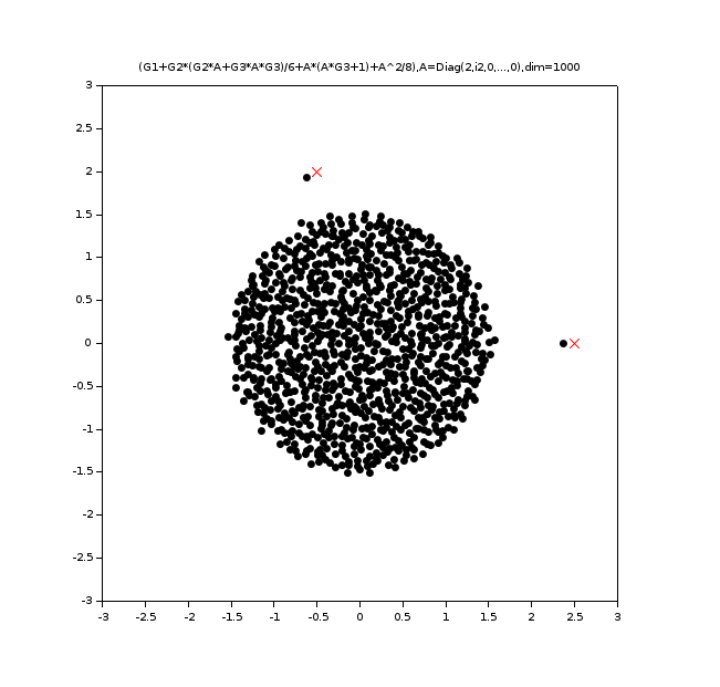
Figure 1: In black, the eigenvalues of P1​(XN(1)N,XN(2)N,XN(3)N,AN)P_{1}\left(\frac{X^{(1)}_{N}}{\sqrt{N}},\frac{X^{(2)}_{N}}{\sqrt{N}},\frac{X^{(3)}_{N}}{\sqrt{N}},A_{N}\right) for N=1000N=1000, and in red, the outliers 2.52.5 and 2​i−0.52i-0.5 of P1​(0N,0N,0N,AN)P_{1}(0_{N},0_{N},0_{N},A_{N}).

The matrix MNM_{N} converges in ∗*-distribution to 32​c\frac{3}{2}c, where cc is a circular variable, and the empirical spectral measure of MNM_{N} converges to the Brown measure of cc, which is the uniform law on the centered disk of radius 3/23/2 by [12]. This disk is also the spectrum of 32​c\frac{3}{2}c. Our theorem says that, outside this disk, the outliers of MNM_{N} are closed to the eigenvalues 2.52.5 and 2​i−0.52i-0.5 of P1​(0N,0N,0N,AN)=AN+18​AN2P_{1}(0_{N},0_{N},0_{N},A_{N})=A_{N}+\frac{1}{8}A_{N}^{2} (see Figure 1).

2.2 Example 2

We consider the matrix

MN=P2​(XN(1)N,XN(2)N,XN(3)N,AN(1),AN(2))\displaystyle M_{N}=P_{2}\left(\frac{X^{(1)}_{N}}{\sqrt{N}},\frac{X^{(2)}_{N}}{\sqrt{N}},\frac{X^{(3)}_{N}}{\sqrt{N}},A_{N}^{(1)},A_{N}^{(2)}\right)
=12​XN(1)N+16​AN(1)​XN(2)N​(AN(2)+AN(1)+XN(3)N)​XN(2)N+AN(2)​XN(3)N​AN(1)\displaystyle=\frac{1}{2}\frac{X^{(1)}_{N}}{\sqrt{N}}+\frac{1}{6}A_{N}^{(1)}\frac{X^{(2)}_{N}}{\sqrt{N}}\left(A_{N}^{(2)}+A_{N}^{(1)}+\frac{X^{(3)}_{N}}{\sqrt{N}}\right)\frac{X^{(2)}_{N}}{\sqrt{N}}+A_{N}^{(2)}\frac{X^{(3)}_{N}}{\sqrt{N}}A_{N}^{(1)}
+AN(1)+12​AN(2),\displaystyle\quad+A_{N}^{(1)}+\frac{1}{2}A_{N}^{(2)},

where XN(1),XN(2),XN(3)X^{(1)}_{N},X^{(2)}_{N},X^{(3)}_{N} are i.i.d. Gaussian matrices,

AN(1)=(2−2.50⋱0)A_{N}^{(1)}=\left(\begin{array}[]{ccccc}2&&&&\\ &-2.5&&&\\ &&0&&\\ &&&\ddots&\\ &&&&0\end{array}\right)

and AN(2)A_{N}^{(2)} is a realization of a G.U.E. matrix.

Refer to caption
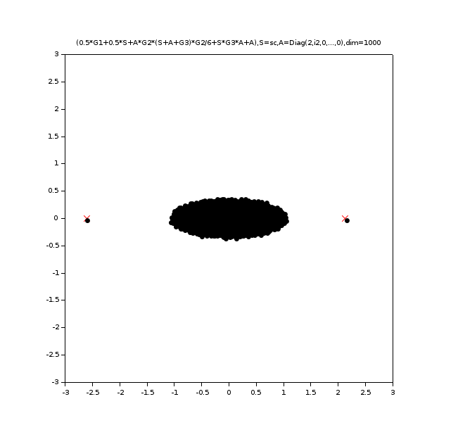
Figure 2: In black, the eigenvalues of P2​(XN(1)N,XN(2)N,XN(3)N,AN(1),AN(2))P_{2}\left(\frac{X^{(1)}_{N}}{\sqrt{N}},\frac{X^{(2)}_{N}}{\sqrt{N}},\frac{X^{(3)}_{N}}{\sqrt{N}},A_{N}^{(1)},A_{N}^{(2)}\right) for N=1000N=1000, and in red, the limiting outliers 2.1252.125 and −2.6-2.6 of P1​(0,0,0,AN(1),AN(2))P_{1}(0,0,0,A_{N}^{(1)},A_{N}^{(2)}).

The matrix MNM_{N} converges in ∗*-distribution to the elliptic variable 12​(c+s)\frac{1}{2}(c+s), where cc is a circular variable and ss a semicircular variable free from cc. The empirical spectral measure of MNM_{N} converges to the Brown measure of 12​(c+s)\frac{1}{2}(c+s), which is the uniform law on the interior of the ellipse {32​2​cos⁡(θ)+i​12​2​sin⁡(θ):0⩽θ<2​π}\{\frac{3}{2\sqrt{2}}\cos(\theta)+i\frac{1}{2\sqrt{2}}\sin(\theta):0\leqslant\theta<2\pi\} by [12]. The interior of this ellipse is also the spectrum of 12​(c+s)\frac{1}{2}(c+s). Our theorem says that, outside this ellipse, the outliers of MNM_{N} are closed to the outliers of P2​(0N,0N,0N,AN(1),AN(2))=AN(1)+12​AN(2)P_{2}(0_{N},0_{N},0_{N},A_{N}^{(1)},A_{N}^{(2)})=A_{N}^{(1)}+\frac{1}{2}A_{N}^{(2)} (see Figure 2). Moreover, the outliers of AN(1)+12​AN(2)A_{N}^{(1)}+\frac{1}{2}A_{N}^{(2)} are those of an additive perturbation of a G.U.E. matrix, and converges to 2.1252.125 and −2.6-2.6 by [28].

2.3 Example 3

We consider the matrix

MN\displaystyle M_{N} =P3​(XN(1)N,XN(2)N,XN(3)N,AN(1),AN(2))\displaystyle=P_{3}\left(\frac{X^{(1)}_{N}}{\sqrt{N}},\frac{X^{(2)}_{N}}{\sqrt{N}},\frac{X^{(3)}_{N}}{\sqrt{N}},A_{N}^{(1)},A_{N}^{(2)}\right)
=XN(1)N+AN(1)+AN(2)+AN(1)​XN(2)N​AN(2)​XN(2)N+XN(3)N​AN(2)​XN(2)N,\displaystyle=\frac{X^{(1)}_{N}}{\sqrt{N}}+A_{N}^{(1)}+A_{N}^{(2)}+A_{N}^{(1)}\frac{X^{(2)}_{N}}{\sqrt{N}}A_{N}^{(2)}\frac{X^{(2)}_{N}}{\sqrt{N}}+\frac{X^{(3)}_{N}}{\sqrt{N}}A_{N}^{(2)}\frac{X^{(2)}_{N}}{\sqrt{N}},

where XN(1),XN(2),XN(3)X^{(1)}_{N},X^{(2)}_{N},X^{(3)}_{N} are i.i.d. Gaussian matrices,

AN(1)=(1⋱1−1⋱−1)A_{N}^{(1)}=\left(\begin{array}[]{cccccc}1&&&&&\\ &\ddots&&&&\\ &&1&&&\\ &&&-1&&\\ &&&&\ddots&\\ &&&&&-1\end{array}\right)

is a matrix whose empirical spectral distribution converges to 12​(δ1+δ−1)\frac{1}{2}(\delta_{1}+\delta_{-1}) and

AN(2)=(1.5−2+2​i0⋱0)A_{N}^{(2)}=\left(\begin{array}[]{ccccc}1.5&&&&\\ &-2+2i&&&\\ &&0&&\\ &&&\ddots&\\ &&&&0\end{array}\right)
Refer to caption
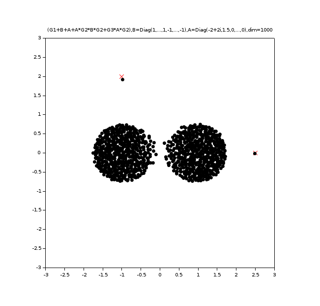
Figure 3: In black, the eigenvalues of P3​(XN(1)N,XN(2)N,XN(3)N,AN(1),AN(2))P_{3}\left(\frac{X^{(1)}_{N}}{\sqrt{N}},\frac{X^{(2)}_{N}}{\sqrt{N}},\frac{X^{(3)}_{N}}{\sqrt{N}},A_{N}^{(1)},A_{N}^{(2)}\right) for N=1000N=1000, and in red, the outliers 2.52.5 and −1+2​i-1+2i of P3​(0N,0N,0N,AN(1),AN(2))P_{3}(0_{N},0_{N},0_{N},A_{N}^{(1)},A_{N}^{(2)}).

The matrix MNM_{N} converges in ∗*-distribution to the random variable c+ac+a, where cc is a circular variable and aa is a self-adjoint random variable, free from cc, and whose distribution is 12​(δ1+δ−1)\frac{1}{2}(\delta_{1}+\delta_{-1}). The empirical spectral measure of MNM_{N} converges to the Brown measure of c+ac+a, which is absolutely continuous and whose support is the region inside the lemniscate-like curve in the complex plane with the equation {z∈ℂ:|z2+1|2=|z|2+1}\{z\in\mathbb{C}:|z^{2}+1|^{2}=|z|^{2}+1\} by [12]. The interior of this ellipse is also the spectrum of c+ac+a. Our theorem says that, outside this ellipse, the outliers of MNM_{N} are closed to the outliers 2.52.5 and −1+2​i-1+2i of P3​(0N,0N,0N,AN(1),AN(2))=AN(1)+AN​(2)P_{3}(0_{N},0_{N},0_{N},A_{N}^{(1)},A_{N}^{(2)})=A_{N}^{(1)}+A_{N}{(2)} (see Figure 3).

2.4 Example 4

We consider the matrix

MN\displaystyle M_{N} =P4​(XN(1)N,XN(2)N,XN(3)N,AN)\displaystyle=P_{4}\left(\frac{X^{(1)}_{N}}{\sqrt{N}},\frac{X^{(2)}_{N}}{\sqrt{N}},\frac{X^{(3)}_{N}}{\sqrt{N}},A_{N}\right)
=15​(XN(1)N+3​IN)​(XN(2)N+AN+2​IN)​(XN(3)N+2​IN)−2​IN,\displaystyle=\frac{1}{5}\left(\frac{X^{(1)}_{N}}{\sqrt{N}}+3I_{N}\right)\left(\frac{X^{(2)}_{N}}{\sqrt{N}}+A_{N}+2I_{N}\right)\left(\frac{X^{(3)}_{N}}{\sqrt{N}}+2I_{N}\right)-2I_{N},

where XN(1),XN(2),XN(3)X^{(1)}_{N},X^{(2)}_{N},X^{(3)}_{N} are i.i.d. Gaussian matrices and

AN=(2​i−2​i0⋱0).A_{N}=\left(\begin{array}[]{ccccc}2i&&&&\\ &-2i&&&\\ &&0&&\\ &&&\ddots&\\ &&&&0\end{array}\right).
Refer to caption
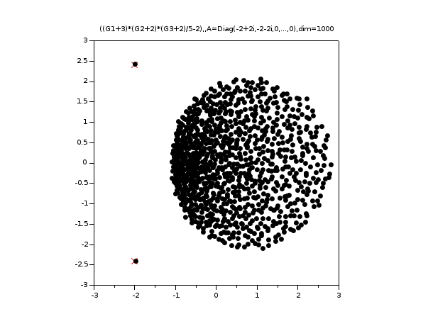
Figure 4: In black, the eigenvalues of P4​(XN(1)N,XN(2)N,XN(3)N,AN)P_{4}\left(\frac{X^{(1)}_{N}}{\sqrt{N}},\frac{X^{(2)}_{N}}{\sqrt{N}},\frac{X^{(3)}_{N}}{\sqrt{N}},A_{N}\right) for N=1000N=1000, and in red, the outliers −2+2.4​i-2+2.4i and −2−2.4​i-2-2.4i of P4​(0N,0N,0N,AN)P_{4}(0_{N},0_{N},0_{N},A_{N}).

The matrix MNM_{N} converges in ∗*-distribution to the random variable (c1+3)​(c2+2)​(c3+2)/5−2(c_{1}+3)(c_{2}+2)(c_{3}+2)/5-2, where c1,c2,c3c_{1},c_{2},c_{3} are free circular variables. It is expected (but not proved) that the empirical spectral measure of MNM_{N} converges to the Brown measure of (c1+3)​(c2+2)​(c3+2)/5−2\left(c_{1}+3\right)\left(c_{2}+2\right)\left(c_{3}+2\right)/5-2. The spectrum of (c1+3)​(c2+2)​(c3+2)/5−2\left(c_{1}+3\right)\left(c_{2}+2\right)\left(c_{3}+2\right)/5-2 is included in the set (B⁡(0,1)+3)​(B⁡(0,1)+2)​(B⁡(0,1)+2)/5−2\left(B(0,1)+3\right)(B(0,1)+2)\left(B(0,1)+2\right)/5-2. Our theorem says that, outside this set, the outliers of MNM_{N} are closed to the outliers −2+2.4​i-2+2.4i and −2−2.4​i-2-2.4i of P4​(0N,0N,0N,AN)=65​AN−2​INP_{4}(0_{N},0_{N},0_{N},A_{N})=\frac{6}{5}A_{N}-2I_{N} (see Figure 4).

3 Free Probability Theory

3.1 Scalar-valued free probability theory

For the reader’s convenience, we recall the following basic definitions from free probability theory. For a thorough introduction to free probability theory, we refer to [42].

  • •

    A 𝒞∗{\cal C}^{*}-probability space is a pair (𝒜,φ)\left({\cal A},\varphi\right) consisting of a unital 𝒞∗{\cal C}^{*}-algebra 𝒜{\cal A} and a state φ\varphi on 𝒜{\cal A} (i.e a linear map φ:𝒜→ℂ\varphi:{\cal A}\rightarrow\mathbb{C} such that φ⁡(1𝒜)=1\varphi(1_{\cal A})=1 and φ⁡(a​a∗)⩾0\varphi(aa^{*})\geqslant 0 for all a∈𝒜a\in{\cal A}) φ\varphi is a trace if it satisfies φ⁡(a​b)=φ⁡(b​a)\varphi(ab)=\varphi(ba) for every (a,b)∈𝒜2(a,b)\in{\cal A}^{2}. A trace is said to be faithful if φ⁡(a​a∗)>0\varphi(aa^{*})>0 whenever a≠0a\neq 0. An element of 𝒜{\cal A} is called a noncommutative random variable.

  • •

    The ∗\ast-noncommutative distribution of a family a=(a1,…,ak)a=(a_{1},\ldots,a_{k}) of noncommutative random variables in a 𝒞∗{\cal C}^{*}-probability space (𝒜,φ)\left({\cal A},\varphi\right) is defined as the linear functional μa:P↦φ⁡(P⁡(a,a∗))\mu_{a}:P\mapsto\varphi(P(a,a^{*})) defined on the set of polynomials in 2​k2k noncommutative indeterminates, where (a,a∗)(a,a^{*}) denotes the 2​k2k-tuple (a1,…,ak,a1∗,…,ak∗)(a_{1},\ldots,a_{k},a_{1}^{*},\ldots,a_{k}^{*}). For any self-adjoint element a1a_{1} in 𝒜{\cal A}, there exists a probability measure νa1\nu_{a_{1}} on ℝ\mathbb{R} such that, for every polynomial P, we have

    μa1​(P)=∫P⁡(t)​d​νa1​(t).\mu_{a_{1}}(P)=\int P(t)\mathrm{d}\nu_{a_{1}}(t).

    Then, we identify μa1\mu_{a_{1}} and νa1\nu_{a_{1}}. If φ\varphi is faithful then the support of νa1\nu_{a_{1}} is the spectrum of a1a_{1} and thus ‖a1‖=sup{|z|,z∈support⁡(νa1)}\|a_{1}\|=\sup\{|z|,z\in\rm{support}(\nu_{a_{1}})\}.

  • •

    A family of elements (ai)i∈I(a_{i})_{i\in I} in a 𝒞∗{\cal C}^{*}-probability space (𝒜,φ)\left({\cal A},\varphi\right) is free if for all k∈ℕk\in\mathbb{N} and all polynomials p1,…,pkp_{1},\ldots,p_{k} in two noncommutative indeterminates, one has

    φ(p1(ai1,ai1∗)⋯pk(aik,aik∗))=0\varphi(p_{1}(a_{i_{1}},a_{i_{1}}^{*})\cdots p_{k}(a_{i_{k}},a_{i_{k}}^{*}))=0 (7)

    whenever i1≠i2,i2≠i3,…,in−1≠iki_{1}\neq i_{2},i_{2}\neq i_{3},\ldots,i_{n-1}\neq i_{k} and φ⁡(pl​(ail,ail∗))=0\varphi(p_{l}(a_{i_{l}},a_{i_{l}}^{*}))=0 for l=1,…,kl=1,\ldots,k.

  • •

    A noncommutative random variable xx in a 𝒞∗{\cal C}^{*}-probability space (𝒜,φ)\left({\cal A},\varphi\right) is a standard semicircular variable if x=x∗x=x^{*} and for any k∈ℕk\in\mathbb{N},

    φ⁡(xk)=∫tk​d​μs​c​(t)\varphi(x^{k})=\int t^{k}d\mu_{sc}(t)

    where d​μs​c​(t)=12​π​4−t2​𝖨[−2;2]​(t)​d​td\mu_{sc}(t)=\frac{1}{2\pi}\sqrt{4-t^{2}}{1\!\!{\sf I}}_{[-2;2]}(t)dt is the semicircular standard distribution.

  • •

    Let kk be a nonnull integer number. Denote by 𝒫{\cal P} the set of polynomials in 2​k2k noncommutative indeterminates. A sequence of families of variables (an)n⩾1=(a1​(n),…,ak​(n))n⩾1(a_{n})_{n\geqslant 1}=(a_{1}(n),\ldots,a_{k}(n))_{n\geqslant 1} in 𝒞∗{\cal C}^{*}-probability spaces (𝒜n,φn)\left({\cal A}_{n},\varphi_{n}\right) converges, when nn goes to infinity, respectively in distribution if the map P∈𝒫↦φn​(P⁡(an,an∗))P\in{\cal P}\mapsto\varphi_{n}(P(a_{n},a_{n}^{*})) converges pointwise.

3.2 Operator-valued free probability theory

3.2.1 Basic definitions

Operator-valued distributions and the operator-valued version of free probability were introduced by Voiculescu in [38] with the main purpose of studying freeness with amalgamation. Thus, an operator-valued noncommutative probability space is a triple (M,E,B)(M,E,B), where MM is a unital algebra over ℂ\mathbb{C}, B⊆MB\subseteq M is a unital subalgebra containing the unit of MM, and E:M→BE\colon M\to B is a unit-preserving conditional expectation, that is, a linear BB-bimodule map such that E⁡[1]=1E[1]=1. We will only need the more restrictive context in which MM is a finite von Neumann algebra which is a factor, BB is a finite-dimensional von Neumann subalgebra of MM (and hence isomorphic to an algebra of matrices), and EE is the unique trace-preserving conditional expectation from MM to BB. The BB-valued distribution of an element X∈MX\in M w.r.t. EE is defined to be the family of multilinear maps called the moments of μX\mu_{X}:

μX={Bn−1∋(b1,b2,…,bn−1)↦E[Xb1Xb2⋯Xbn−1X]∈B:n≥0},\mu_{X}=\{B^{n-1}\ni(b_{1},b_{2},\dots,b_{n-1})\mapsto E[Xb_{1}Xb_{2}\cdots Xb_{n-1}X]\in B\colon n\geq 0\},

with the convention that the first moment (corresponding to n=1n=1) is the element E⁡[X]∈BE[X]\in B, and the zeroth moment (corresponding to n=0n=0) is the unit 11 of BB (or MM). The distribution of XX is encoded conveniently by a noncommutative analytic transform defined for certain elements b∈Bb\in B, which we agree to call the noncommutative Cauchy transform:

GX​(b)=E⁡[(X−b)−1].G_{X}(b)=E\left[(X-b)^{-1}\right].

(To be more precise, it is the noncommutative extension GX⊗1n​(b)=(E⊗Idℳn​(B))​[(X⊗1n−b)−1]G_{X\otimes 1_{n}}(b)=(E\otimes{\rm Id}_{{\cal M}_{n}(B)})\left[(X\otimes 1_{n}-b)^{-1}\right], for elements B∈ℳn​(B)B\in{\cal M}_{n}(B), which completely encodes μX\mu_{X} - see [41]; since we do not need this extension, we shall not discuss it any further, but refer the reader to [41, 39, 40, 29] for details.) A natural domain for GXG_{X} is the upper half-plane of BB, H+​(B)={b∈B:ℑ⁡b>0}H^{+}(B)=\{b\in B\colon\Im b>0\}. It follows quite easily that GX​(H+​(B))⊆H+​(B)G_{X}(H^{+}(B))\subseteq H^{+}(B) - see [40].

We warn here the reader that we have changed conventions in our paper compared to [39, 40, 41], namely we have chosen GX​(b)=E⁡[(X−b)−1]G_{X}(b)=E\left[(X-b)^{-1}\right] instead of E⁡[(b−X)−1]E\left[(b-X)^{-1}\right], so that GXG_{X} preserves H+​(B)H^{+}(B).

Among many other results proved in [38], one can find a central limit theorem for random variables which are free with amalgamation. The central limit distribution is called an operator-valued semicircular, by analogy with the free central limit for the usual, scalar-valued random variables, which is Wigner’s semicircular distribution. It has been shown in [38] that an operator-valued semicircular distribution is entirely described by its operator-valued free cumulants: only the first and second cumulants of an operator-valued semicircular distribution may be nonzero (see also [33, 41]). For our purposes, we use the equivalent description of an operator-valued semicircular distribution via its noncommutative Cauchy transform, as in [22]: SS is a BB-valued semicircular if and only if

GS​(b)=(m1−b−η⁡(GS​(b)))−1,b∈H+​(B),G_{S}(b)=\left(m_{1}-b-\eta(G_{S}(b))\right)^{-1},\quad b\in H^{+}(B),

for some m1=m1∗∈Bm_{1}=m_{1}^{*}\in B and completely positive map η:B→B\eta\colon B\to B. In that case, m1=E⁡[S]m_{1}=E[S] and η⁡(b)=E⁡[S​b​S]−E⁡[S]​b​E​[S]\eta(b)=E[SbS]-E[S]bE[S]. The above equation is obviously a generalization of the quadratic equation determining Wigner’s semicircular distribution: σ2​GS​(z)2+(z−m1)​GS​(z)+1=0\sigma^{2}G_{S}(z)^{2}+(z-m_{1})G_{S}(z)+1=0. Here m1m_{1} is the - classical - first moment of SS, and σ2\sigma^{2} its classical variance, which, as a linear completely positive map, is the multiplication with a positive constant. Unless otherwise specified, we shall from now on assume our semicirculars to be centered, i.e. m1=0m_{1}=0.

Example 13.

A rich source of examples of operator-valued semicirculars comes in the case of finite dimensional BB from scalar-valued semicirculars: assume that si,j,1≤i≤j≤ns_{i,j},1\leq i\leq j\leq n are scalar-valued centered semicircular random variables of variance one. We do not assume them to be free. Then the matrix

[α1​s1,1γ1,2​s1,2γ1,3​s1,3⋯γ1,n−1​s1,n−1γ1,n​s1,nγ1,2¯​s1,2α2​s2,2γ2,3​s2,3⋯γ2,n−1​s2,n−1γ2,n​s2,nγ1,3¯​s1,3γ2,3¯​s2,3α3​s3,3⋯γ3,n−1​s3,n−1γ3,n​s3,n⋱γ1,n−1¯​s1,n−1γ2,n−1¯​s2,n−1γ3,n−1¯​s3,n−1⋯αn−1​sn−1,n−1γn−1,n​sn−1,nγ1,n¯​s1,nγ2,n¯​s2,nγ3,n¯​s3,n⋯γn−1,n¯​sn−1,nαn​sn,n],\begin{bmatrix}\alpha_{1}s_{1,1}&\gamma_{1,2}s_{1,2}&\gamma_{1,3}s_{1,3}&\cdots&\gamma_{1,n-1}s_{1,n-1}&\gamma_{1,n}s_{1,n}\\ \overline{\gamma_{1,2}}s_{1,2}&\alpha_{2}s_{2,2}&\gamma_{2,3}s_{2,3}&\cdots&\gamma_{2,n-1}s_{2,n-1}&\gamma_{2,n}s_{2,n}\\ \overline{\gamma_{1,3}}s_{1,3}&\overline{\gamma_{2,3}}s_{2,3}&\alpha_{3}s_{3,3}&\cdots&\gamma_{3,n-1}s_{3,n-1}&\gamma_{3,n}s_{3,n}\\ \vdots&\vdots&\vdots&\ddots&\vdots&\vdots\\ \overline{\gamma_{1,n-1}}s_{1,n-1}&\overline{\gamma_{2,n-1}}s_{2,n-1}&\overline{\gamma_{3,n-1}}s_{3,n-1}&\cdots&\alpha_{n-1}s_{n-1,n-1}&\gamma_{n-1,n}s_{n-1,n}\\ \overline{\gamma_{1,n}}s_{1,n}&\overline{\gamma_{2,n}}s_{2,n}&\overline{\gamma_{3,n}}s_{3,n}&\cdots&\overline{\gamma_{n-1,n}}s_{n-1,n}&\alpha_{n}s_{n,n}\end{bmatrix},

where α1,…,αn∈[0,+∞)\alpha_{1},\dots,\alpha_{n}\in[0,+\infty) and γi,j∈ℂ\gamma_{i,j}\in\mathbb{C}, 1≤i<j≤n1\leq i<j\leq n, is an ℳn​(ℂ){\cal M}_{n}(\mathbb{C})-valued semicircular. Note that we do allow our scalars to be zero. This is a particular case of a result from [30], and its proof can be found in great detail in [25].

An important fact about semicircular elements, both scalar- and operator-valued, is that the sum of two free semicircular elements is again a semicircular element (this follows from the fact that a semicircular is defined by having all its cumulants beyond the first two equal to zero - see [38]). In particular, if {s1,1(1),s1,2(1),s2,2(1),s1,1(2),s1,2(2),s2,2(2)}\{s_{1,1}^{(1)},s_{1,2}^{(1)},s_{2,2}^{(1)},s_{1,1}^{(2)},s_{1,2}^{(2)},s_{2,2}^{(2)}\} are centered all semicirculars of variance one, and in addition we assume them to be free from each other, then [s1,1(1)s1,2(1)s1,2(1)s2,2(1)]\begin{bmatrix}s_{1,1}^{(1)}&s_{1,2}^{(1)}\\ s_{1,2}^{(1)}&s_{2,2}^{(1)}\end{bmatrix} and [s1,1(2)i​s1,2(2)−i​s1,2(2)s2,2(2)]\begin{bmatrix}s_{1,1}^{(2)}&is_{1,2}^{(2)}\\ -is_{1,2}^{(2)}&s_{2,2}^{(2)}\end{bmatrix} are ℳ2​(ℂ){\cal M}_{2}(\mathbb{C})-valued semicirculars which are free over ℳ2​(ℂ){\cal M}_{2}(\mathbb{C}), so their sum [s1,1(1)+s1,1(2)s1,2(1)+i​s1,2(2)s1,2(1)−i​s1,2(2)s2,2(1)+s2,2(2)]\begin{bmatrix}s_{1,1}^{(1)}+s_{1,1}^{(2)}&s_{1,2}^{(1)}+is_{1,2}^{(2)}\\ s_{1,2}^{(1)}-is_{1,2}^{(2)}&s_{2,2}^{(1)}+s_{2,2}^{(2)}\end{bmatrix} is also an ℳ2​(ℂ){\cal M}_{2}(\mathbb{C})-valued semicircular, despite its off-diagonal elements not being anymore distributed according to the Wigner semicircular law. This is hardly surprising: the two matrices we have added are the limits of the real and imaginary parts of a G.U.E. (Gaussian Unitary Ensemble). The upper right corner of a G.U.E. is known to be a C.U.E. (Circular Unitary Ensemble), and its eigenvalues converge to the uniform law on a disk. On the other hand, direct analytic computations show that the sum s1,2(1)±i​s1,2(2)s_{1,2}^{(1)}\pm is_{1,2}^{(2)}, with s1,2(1)s_{1,2}^{(1)} and s1,2(2)s_{1,2}^{(2)} free from each other, has precisely the same law. Thus, the following definition, due to Voiculescu, is natural.

Definition 14.

An element cc in a ∗-noncommutative probability space (𝒜,φ)(\mathcal{A},\varphi) is called a circular random variable if (c+c∗)/2(c+c^{*})/\sqrt{2} and (c−c∗)/2​i(c-c^{*})/\sqrt{2}i, respectively, are free from each other and identically distributed according to standard Wigner’s semicircular law.

3.2.2 Preliminary results

We first establish preliminary results in free probability theory that we will need in the following sections.

Lemma 15.

Let {mp(j),p=1,…,4,j=1,…,t}\{m_{p}^{(j)},p=1,\ldots,4,j=1,\ldots,t\} be noncommutative random variables in some noncommutative probability space (𝒜,φ)(\mathcal{A},\varphi). Let si(1)s_{i}^{(1)}, si(2)s_{i}^{(2)},i=1,…,ui=1,\ldots,u be semicircular variables and cic_{i},i=1,…,ui=1,\ldots,u be circular variables such that s1(1),…,su(1),s1(2),…,su(2),c1,…,cu,{mp(j),p=1,…,4,j=1,…,t}s_{1}^{(1)},\ldots,s_{u}^{(1)},s_{1}^{(2)},\ldots,s_{u}^{(2)},c_{1},\ldots,c_{u},\{m_{p}^{(j)},p=1,\ldots,4,j=1,\ldots,t\} are ∗\ast-free in (𝒜,φ)(\mathcal{A},\varphi). Define for i=1,…,ui=1,\ldots,u,

𝐬𝐢=12​(si(1)cici∗si(2)),{\bf s_{i}}=\frac{1}{\sqrt{2}}\begin{pmatrix}s_{i}^{(1)}&c_{i}\\ c_{i}^{*}&s_{i}^{(2)}\end{pmatrix},

and for j=1,…,tj=1,\ldots,t,

𝐦𝐣=(m1(j)m2(j)m3(j)m4(j)).{\bf m_{j}}=\begin{pmatrix}m_{1}^{(j)}&m_{2}^{(j)}\\ m_{3}^{(j)}&m_{4}^{(j)}\end{pmatrix}.

Then, in the scalar-valued probability space (ℳ2​(𝒜),tr2⊗φ)({\cal M}_{2}(\mathcal{A}),\operatorname{tr}_{2}\otimes\varphi), 𝐬𝟏,…,𝐬𝐮,{𝐦𝐣,j=1,…,t}{\bf s_{1}},\ldots,{\bf s_{u}},\{{\bf m_{j}},j=1,\ldots,t\} are free and for i=1,…,ui=1,\ldots,u, each 𝐬𝐢{\bf s_{i}} is a semicircular variable.

Proof.

Let us prove that 𝐬𝟏,…,𝐬𝐮{\bf s_{1}},\ldots,{\bf s_{u}} is free from ℳ2​(ℬ)\mathcal{M}_{2}(\mathcal{B}), where ℬ\mathcal{B} is the ∗\ast-algebra generated by {mp(j),p=1,…,4,j=1,…,t}\{m_{p}^{(j)},p=1,\ldots,4,j=1,\ldots,t\}. We already now (see [25, Chapter 9]) that 𝐬𝟏,…,𝐬𝐮{\bf s_{1}},\ldots,{\bf s_{u}} are semicircular variables over ℳ2​(ℂ)\mathcal{M}_{2}(\mathbb{C}) which are free from ℳ2​(ℬ)\mathcal{M}_{2}(\mathcal{B}), with respect to i​d2⊗φid_{2}\otimes\varphi. Moreover, the covariance mapping of 𝐬𝟏,…,𝐬𝐮{\bf s_{1}},\ldots,{\bf s_{u}} is the function (ηi,jℳ2​(ℂ):ℳ2(ℂ)→ℳ2(ℂ))1⩽i,j⩽u(\eta^{\mathcal{M}_{2}(\mathbb{C})}_{i,j}:{\cal M}_{2}(\mathbb{C})\to{\cal M}_{2}(\mathbb{C}))_{1\leqslant i,j\leqslant u}, which can be computed as follows: for all m=(m1m2m3m4)∈ℳ2​(ℂ),m=\left(\begin{array}[]{cc}m_{1}&m_{2}\\ m_{3}&m_{4}\end{array}\right)\in{\cal M}_{2}(\mathbb{C}), we have

ηi,jℳ2​(ℂ)​(m)\displaystyle\eta^{\mathcal{M}_{2}(\mathbb{C})}_{i,j}(m) =(id2⊗φ)​(𝐬i​m​𝐬j)\displaystyle=(\id_{2}\otimes\varphi)({\bf s}_{i}m{\bf s}_{j})
=12​(φ⁡(si(1)​m1​sj(1))+φ⁡(si(1)​m2​cj∗)+φ⁡(ci​m3​sj(1))+φ⁡(ci​m4​cj∗)⋆⋆⋆)\displaystyle=\frac{1}{2}\left(\begin{array}[]{c|c}\varphi(s_{i}^{(1)}m_{1}s_{j}^{(1)})+\varphi(s_{i}^{(1)}m_{2}c_{j}^{*})+\varphi(c_{i}m_{3}s_{j}^{(1)})+\varphi(c_{i}m_{4}c_{j}^{*})&\star\\ \hline\cr\star&\star\\ \end{array}\right)
=δi​j2​(m1+m400m1+m4)\displaystyle=\frac{\delta_{ij}}{2}\left(\begin{array}[]{c|c}m_{1}+m_{4}&0\\ \hline\cr 0&m_{1}+m_{4}\\ \end{array}\right)
=δi​j​tr2⁡(m)​I2.\displaystyle=\delta_{ij}\operatorname{tr}_{2}(m)I_{2}.

Using [26, Theorem 3.5], the freeness of 𝐬𝟏,…,𝐬𝐮{\bf s_{1}},\ldots,{\bf s_{u}} from ℳ2​(ℬ){\cal M}_{2}(\mathcal{B}) over ℳ2​(ℂ){\cal M}_{2}(\mathbb{C}) gives us the free cumulants of 𝐬𝟏,…,𝐬𝐮{\bf s_{1}},\ldots,{\bf s_{u}} over ℳ2​(ℬ){\cal M}_{2}(\mathcal{B}). More concretely, we get that 𝐬𝟏,…,𝐬𝐮{\bf s_{1}},\ldots,{\bf s_{u}} are semicircular variables over ℳ2​(ℬ){\cal M}_{2}(\mathcal{B}), with a covariance mapping (ηi,jℳ2​(ℬ):ℳ2(ℬ)→ℳ2(ℬ))1⩽i,j⩽u(\eta^{{\cal M}_{2}(\mathcal{B})}_{i,j}:{\cal M}_{2}(\mathcal{B})\to{\cal M}_{2}(\mathcal{B}))_{1\leqslant i,j\leqslant u} given by ηi,jℳ2​(ℬ)=ηi,jℳ2​(ℂ)∘(i​d2⊗φ)\eta^{{\cal M}_{2}(\mathcal{B})}_{i,j}=\eta^{{\cal M}_{2}(\mathbb{C})}_{i,j}\circ(id_{2}\otimes\varphi).

Because of the previous computation, we know that ηi,jℳ2​(ℂ)=tr2∘ηi,jℳ2​(ℂ)∘tr2\eta^{{\cal M}_{2}(\mathbb{C})}_{i,j}=\operatorname{tr}_{2}\circ\eta^{{\cal M}_{2}(\mathbb{C})}_{i,j}\circ\operatorname{tr}_{2}, which means that ηi,jℳ2​(ℬ)=(tr2⊗φ)∘ηi,jℳ2​(ℬ)∘(tr2⊗φ)\eta^{{\cal M}_{2}(\mathcal{B})}_{i,j}=(\operatorname{tr}_{2}\otimes\varphi)\circ\eta^{{\cal M}_{2}(\mathcal{B})}_{i,j}\circ(\operatorname{tr}_{2}\otimes\varphi). As a consequence, using again [26, Theorem 3.5], 𝐬𝟏,…,𝐬𝐮{\bf s_{1}},\ldots,{\bf s_{u}} are semicircular variables over ℂ\mathbb{C} free from M2​(ℬ)M_{2}(\mathcal{B}) with respect to (tr2⊗φ)(\operatorname{tr}_{2}\otimes\varphi), and the covariance mapping ηi,jℂ\eta^{\mathbb{C}}_{i,j} is given by the restriction of the covariance mapping ηℳ2​(ℂ)\eta^{{\cal M}_{2}(\mathbb{C})} to ℂ\mathbb{C}: for all m∈ℂm\in\mathbb{C}

ηi,jℂ​(m)=δi​j​m,\eta^{\mathbb{C}}_{i,j}(m)=\delta_{ij}m,

which means that 𝐬𝟏,…,𝐬𝐮{\bf s_{1}},\ldots,{\bf s_{u}} are free standard semicircular variables. ∎

Lemma 16.

Let yy be a noncommutative random variable in ℳm​(𝒜){\cal M}_{m}({\cal A}) and c(1),…,c(u)c^{(1)},\dots,c^{(u)} be free circular variables in 𝒜{\cal A} free from the entries of yy. Then, in the operator-valued probability space (ℳm​(𝒜),i​dm⊗φ)({\cal M}_{m}({\cal A}),id_{m}\otimes\varphi), |∑j=1uζj⊗c(j)+y|2|\sum_{j=1}^{u}\zeta_{j}\otimes c^{(j)}+y|^{2} has the same distribution as |∑j=1uζj⊗sj+(Im⊗ϵ)⋅y|2|\sum_{j=1}^{u}\zeta_{j}\otimes s_{j}+(I_{m}\otimes\epsilon)\cdot y|^{2} where ϵ\epsilon is a selfadjoint {−1,+1}\{-1,+1\}-Bernoulli variable in 𝒜{\cal A}, independent from the entries of yy, and s1,…,sus_{1},\ldots,s_{u} are free semicircular variables in 𝒜{\cal A}, free from ϵ\epsilon and the entries of yy.

In the lemma above, we consider the symmetric version ϵ​y\epsilon y of yy, thanks to a noncommutative random variable ϵ\epsilon which is tensor-independent from the entries of yy, in the sense that ϵ\epsilon commutes with the entries of yy and φ(p1(ϵ)p2(yi,j,yi,j∗:i,j))=φ(p1(ϵ))φ(p2(yi,j,yi,j∗:i,j))\varphi(p_{1}(\epsilon)p_{2}(y_{i,j},y^{*}_{i,j}:i,j))=\varphi(p_{1}(\epsilon))\varphi(p_{2}(y_{i,j},y^{*}_{i,j}:i,j)) for all polynomials p1,p2p_{1},p_{2}.

Proof.

Let n⩾0n\geqslant 0. We compute the nn-th moment of |∑j=1uζj⊗c(j)+y|2|\sum_{j=1}^{u}\zeta_{j}\otimes c^{(j)}+y|^{2} with respect to i​dm⊗φid_{m}\otimes\varphi, and compare it to the nn-th moment of |∑j=1uζj⊗sj+ϵ​y|2|\sum_{j=1}^{u}\zeta_{j}\otimes s_{j}+\epsilon y|^{2} with respect to i​dm⊗φid_{m}\otimes\varphi.

Let us set a0=ya_{0}=y and aj=ζj⊗c(j)a_{j}=\zeta_{j}\otimes c^{(j)}. We compute

i​dm⊗φ⁡(|∑j=1uζj⊗c(j)+y|2​n)\displaystyle id_{m}\otimes\varphi(|\sum_{j=1}^{u}\zeta_{j}\otimes c^{(j)}+y|^{2n})
=∑0⩽i1,…,i2​n⩽ui​dm⊗φ⁡(ai1​ai2∗​ai3​ai4∗​…​ai2​n−1​ai2​n∗).\displaystyle=\sum_{0\leqslant i_{1},\ldots,i_{2n}\leqslant u}id_{m}\otimes\varphi(a_{i_{1}}a_{i_{2}}^{*}a_{i_{3}}a_{i_{4}}^{*}\ldots a_{i_{2n-1}}a_{i_{2n}}^{*}).

Similarly,

i​dm⊗φ⁡(|∑j=1uζj⊗sj+(Im⊗ϵ)⋅y|2​n)\displaystyle id_{m}\otimes\varphi(|\sum_{j=1}^{u}\zeta_{j}\otimes s_{j}+(I_{m}\otimes\epsilon)\cdot y|^{2n})
=∑0⩽i1,…,i2​n⩽ui​dm⊗φ⁡(bi1​bi2∗​bi3​bi4∗​…​bi2​n−1​bi2​n∗).\displaystyle=\sum_{0\leqslant i_{1},\ldots,i_{2n}\leqslant u}id_{m}\otimes\varphi(b_{i_{1}}b_{i_{2}}^{*}b_{i_{3}}b_{i_{4}}^{*}\ldots b_{i_{2n-1}}b_{i_{2n}}^{*}).

where b0=(Im⊗ϵ)⋅yb_{0}=(I_{m}\otimes\epsilon)\cdot y and bj=ζj⊗sjb_{j}=\zeta_{j}\otimes s_{j}. In order to conclude, it suffices to prove that, for all 0⩽i1,…,i2​n⩽u0\leqslant i_{1},\ldots,i_{2n}\leqslant u,

i​dm⊗φ⁡(ai1​ai2∗​ai3​ai4∗​…​ai2​n−1​ai2​n∗)=i​dm⊗φ⁡(bi1​bi2∗​bi3​bi4∗​…​bi2​n−1​bi2​n∗).id_{m}\otimes\varphi(a_{i_{1}}a_{i_{2}}^{*}a_{i_{3}}a_{i_{4}}^{*}\ldots a_{i_{2n-1}}a_{i_{2n}}^{*})=id_{m}\otimes\varphi(b_{i_{1}}b_{i_{2}}^{*}b_{i_{3}}b_{i_{4}}^{*}\ldots b_{i_{2n-1}}b_{i_{2n}}^{*}).

Let us fix 0⩽i1,…,i2​n⩽u0\leqslant i_{1},\ldots,i_{2n}\leqslant u. Note that a0a_{0} is free over ℳm​(ℂ){\cal M}_{m}(\mathbb{C}) from aja_{j} with respect to i​dm⊗φid_{m}\otimes\varphi (see [25, Chapter 9]). Let us fix S={j:ij≠0}⊂{1,…,2​n}S=\{j:i_{j}\neq 0\}\subset\{1,\ldots,2n\} and use the moment cumulant formula (see [33, page 36]):

i​dm⊗φ⁡(ai1​ai2∗​ai3​ai4∗​…​ai2​n−1​ai2​n∗)\displaystyle id_{m}\otimes\varphi(a_{i_{1}}a_{i_{2}}^{*}a_{i_{3}}a_{i_{4}}^{*}\ldots a_{i_{2n-1}}a_{i_{2n}}^{*})
=∑π∈N​C​(S)(c^∪φ^)​(π∪πc)​(ai1⊗ai2∗​…​ai2​n−1⊗ai2​n∗)\displaystyle=\sum_{\pi\in NC(S)}(\hat{c}\cup\hat{\varphi})(\pi\cup\pi^{c})(a_{i_{1}}\otimes a_{i_{2}}^{*}\ldots a_{i_{2n-1}}\otimes a_{i_{2n}}^{*})

where πc\pi^{c} is the largest partition of ScS^{c} such that π∪πc\pi\cup\pi^{c} is noncrossing and c^\hat{c} and φ^\hat{\varphi} are the ℳm​(ℂ){\cal M}_{m}(\mathbb{C})-valued cumulant function and the ℳm​(ℂ){\cal M}_{m}(\mathbb{C})-valued moment function associated to the conditional expectation i​dm⊗φid_{m}\otimes\varphi. We use here the notation of [33, Notation 2.1.4] which defines (c^∪φ^)​(π∪πc)(\hat{c}\cup\hat{\varphi})(\pi\cup\pi^{c}) as some ℳm​(ℂ){\cal M}_{m}(\mathbb{C})-valued multiplicative function that acts on the blocks of π\pi like c^\hat{c} and on the blocks of πc\pi^{c} like φ^\hat{\varphi}.

Recall that the cumulants of ζj⊗c(j)\zeta_{j}\otimes c^{(j)} are vanishing if π\pi is not a pairing and if π\pi is not alternating (which means that π\pi links two indices with the same parity). Now, let us remark that if π\pi is a pairing which is alternating, then πc\pi^{c} is even (each blocs of πc\pi^{c} is even). Thus,

i​dm⊗φ⁡(ai1​ai2∗​ai3​ai4∗​…​ai2​n−1​ai2​n∗)\displaystyle id_{m}\otimes\varphi(a_{i_{1}}a_{i_{2}}^{*}a_{i_{3}}a_{i_{4}}^{*}\ldots a_{i_{2n-1}}a_{i_{2n}}^{*})
=∑π∈N​C​(S)π​ pairing and alternating(c^∪φ^)​(π∪πc)​(ai1⊗ai2∗​…​ai2​n−1⊗ai2​n∗)\displaystyle=\sum_{\begin{subarray}{c}\pi\in NC(S)\\ \pi\text{ pairing and alternating}\end{subarray}}(\hat{c}\cup\hat{\varphi})(\pi\cup\pi^{c})(a_{i_{1}}\otimes a_{i_{2}}^{*}\ldots a_{i_{2n-1}}\otimes a_{i_{2n}}^{*})
=∑π∈N​C​(S)π​ pairing and alternatingπc​ even(c^∪φ^)​(π∪πc)​(ai1⊗ai2∗​…​ai2​n−1⊗ai2​n∗).\displaystyle=\sum_{\begin{subarray}{c}\pi\in NC(S)\\ \pi\text{ pairing and alternating}\\ \pi^{c}\text{ even}\end{subarray}}(\hat{c}\cup\hat{\varphi})(\pi\cup\pi^{c})(a_{i_{1}}\otimes a_{i_{2}}^{*}\ldots a_{i_{2n-1}}\otimes a_{i_{2n}}^{*}).

Similarly, the cumulants of ζj⊗s(j)\zeta_{j}\otimes s^{(j)} are vanishing if π\pi is not a pairing and that the moment of b0b_{0} is vanishing if πc\pi^{c} is odd. Moreover, if π\pi is a pairing and πc\pi^{c} is even, then π\pi is alternating. As a consequence,

i​dm⊗φ⁡(bi1​bi2∗​bi3​bi4∗​…​bi2​n−1​bi2​n∗)\displaystyle id_{m}\otimes\varphi(b_{i_{1}}b_{i_{2}}^{*}b_{i_{3}}b_{i_{4}}^{*}\ldots b_{i_{2n-1}}b_{i_{2n}}^{*})
=∑π∈N​C​(S)(c^∪φ^)​(π∪πc)​(bi1⊗bi2∗​…​bi2​n−1⊗bi2​n∗)\displaystyle=\sum_{\pi\in NC(S)}(\hat{c}\cup\hat{\varphi})(\pi\cup\pi^{c})(b_{i_{1}}\otimes b_{i_{2}}^{*}\ldots b_{i_{2n-1}}\otimes b_{i_{2n}}^{*})
=∑π∈N​C​(S)π​ pairingπc​ even(c^∪φ^)​(π∪πc)​(bi1⊗bi2∗​…​bi2​n−1⊗bi2​n∗)\displaystyle=\sum_{\begin{subarray}{c}\pi\in NC(S)\\ \pi\text{ pairing}\\ \pi^{c}\text{ even}\end{subarray}}(\hat{c}\cup\hat{\varphi})(\pi\cup\pi^{c})(b_{i_{1}}\otimes b_{i_{2}}^{*}\ldots b_{i_{2n-1}}\otimes b_{i_{2n}}^{*})
=∑π∈N​C​(S)π​ pairing and alternatingπc​ even(c^∪φ^)​(π∪πc)​(bi1⊗bi2∗​…​bi2​n−1⊗bi2​n∗).\displaystyle=\sum_{\begin{subarray}{c}\pi\in NC(S)\\ \pi\text{ pairing and alternating}\\ \pi^{c}\text{ even}\end{subarray}}(\hat{c}\cup\hat{\varphi})(\pi\cup\pi^{c})(b_{i_{1}}\otimes b_{i_{2}}^{*}\ldots b_{i_{2n-1}}\otimes b_{i_{2n}}^{*}).

In order to conclude, it suffices to remark that ϵ​y\epsilon y and yy has the same even ℳm​(ℂ){\cal M}_{m}(\mathbb{C})-valued moments and ζj⊗c(j)\zeta_{j}\otimes c^{(j)} and ζj⊗s(j)\zeta_{j}\otimes s^{(j)} has the same alternating ℳm​(ℂ){\cal M}_{m}(\mathbb{C})-valued cumulants. ∎

It follows from [4] that the support in ℳm​(ℂ)sa{\cal M}_{m}(\mathbb{C})^{\rm sa} of the addition of a semicircular ss of variance η\eta and a selfadjoint noncommutative random variable y∈(ℳm​(𝒜),i​dm⊗φ)y\in({\cal M}_{m}({\cal A}),id_{m}\otimes\varphi) which is free with amalgamation over ℳm​(ℂ){\cal M}_{m}(\mathbb{C}) with ss, is given via its complement in terms of yy and the functions

H⁡(w)=w−η⁡(Gy​(w))​ and ​ω​(b)=b+η⁡(Gy​(ω⁡(b))CLOSE,H(w)=w-\eta(G_{y}(w))\text{ and }\omega(b)=b+\eta(G_{y}(\omega(b)), (8)

where Gx​(b)=i​dm⊗φ⁡[(x−b)−1]G_{x}(b)=id_{m}\otimes\varphi\left[(x-b)^{-1}\right].

Proposition 17.

If w∈ℳm​(ℂ)saw\in{\cal M}_{m}(\mathbb{C})^{\rm sa} is such that y−wy-w is invertible and spect​(η∘Gy′​(w))⊂𝔻¯∖{1}\text{spect}(\eta\circ G_{y}^{\prime}(w))\subset\overline{\mathbb{D}}\setminus\{1\}, then s+y−H⁡(w)s+y-H(w) is invertible. Conversely, if b∈ℳm​(ℂ)sab\in{\cal M}_{m}(\mathbb{C})^{\rm sa} is such that s+y−bs+y-b is invertible, then y−ω⁡(b)y-\omega(b) is invertible.

It follows quite easily that spect​(η∘Gy′​(ω⁡(b)))⊂𝔻¯\text{spect}(\eta\circ G_{y}^{\prime}(\omega(b)))\subset\overline{\mathbb{D}}. Generally, all conditions on the derivatives of ω\omega and HH follow from the two functional equations above.

Proof.

Assume that y−wy-w is invertible and spect​(η∘Gy′​(w))⊂𝔻¯∖{1}\text{spect}(\eta\circ G_{y}^{\prime}(w))\subset\overline{\mathbb{D}}\setminus\{1\}. Since w=w∗w=w^{*}, the derivative Gy′​(w)G^{\prime}_{y}(w) is completely positive, so η∘Gy′​(w)\eta\circ G_{y}^{\prime}(w) is completely positive. This means according to [17, Theorem 2.5] that the spectral radius rr of η∘Gy′​(w)\eta\circ G_{y}^{\prime}(w) is reached at a positive element ξ∈Mm​(ℂ)\xi\in M_{m}(\mathbb{C}), so that necessarily r≥0r\geq 0. Since 1∉σ⁡(η∘Gy′​(w))1\not\in\sigma(\eta\circ G_{y}^{\prime}(w)) by hypothesis, it follows that r<1r<1, and thus

spect​(η∘Gy′​(w))⊆r​𝔻¯⊊𝔻.\text{spect}(\eta\circ G_{y}^{\prime}(w))\subseteq r\overline{\mathbb{D}}\subsetneq\mathbb{D}.

This forces the derivative of H⁡(w)H(w), OPENH′​(w)=IdMm​(ℂ)−η∘Gy′​(w))H^{\prime}(w)=\mathrm{Id}_{M_{m}(\mathbb{C})}-\eta\circ G^{\prime}_{y}(w)), to be invertible as a linear operator from ℳm​(ℂ){\cal M}_{m}(\mathbb{C}) to itself. By the inverse function theorem, HH has an analytic inverse on a small enough neighborhood of H⁡(w)H(w) onto a neighborhood of ww. Since HH preserves the selfadjoints near ww, so must the inverse. On the other hand, the map v↦H⁡(w)+η⁡(Gy​(v))v\mapsto H(w)+\eta(G_{y}(v)) sends the upper half-plane into itself and has ww as a fixed point. Since its derivative has all its eigenvalues included strictly in 𝔻\mathbb{D} (recall that the spectral radius r<1r<1), it follows that ww is actually an attracting fixed point for this map. Since for any bb in the upper half-plane, ω⁡(b)\omega(b) is given as the attracting fixed point of v↦b+η⁡(Gy​(v))v\mapsto b+\eta(G_{y}(v)), it follows that ω\omega coincides with the local inverse of HH on the upper half-plane, so the local inverse of HH is the unique analytic continuation of ω\omega to a neighborhood of H⁡(w)H(w). This proves that ω\omega extends analytically to a neighborhood of H⁡(w)H(w) and the extension maps selfadjoints from this neighborhood to ℳm​(ℂ)sa{\cal M}_{m}(\mathbb{C})^{\rm sa}. In particular, ω⁡(H⁡(v))=v\omega(H(v))=v and Gs+y​(H⁡(v))=Gy​(ω⁡(H⁡(v)))=Gy​(v)G_{s+y}(H(v))=G_{y}(\omega(H(v)))=G_{y}(v) are selfadjoint for all v=v∗v=v^{*} in a small enough neighborhood of ww, showing that s+y−H⁡(w)s+y-H(w) is invertible.

Conversely, say b=b∗b=b^{*} and s+y−bs+y-b is invertible. Then Gs+yG_{s+y} is analytic on a neighborhood of bb and maps selfadjoints from this neighborhood into ℳm​(ℂ)sa{\cal M}_{m}(\mathbb{C})^{\rm sa}. Since ω⁡(b)=b+η⁡(Gs+y​(b))\omega(b)=b+\eta(G_{s+y}(b)), the same holds for ω\omega. Since, by [4, Proposition 4.1], spect(ω′(v))⊂{ℜz>1/2}\text{spect}(\omega^{\prime}(v))\subset\{\Re z>1/2\} for any vv in the upper half-plane, the analyticity of ω\omega around b=b∗b=b^{*} implies spect(ω′(0))⊂{ℜz≥1/2}\text{spect}(\omega^{\prime}(0))\subset\{\Re z\geq 1/2\}. Thus, ω\omega is invertible wrt composition around zero by the inverse function theorem. As argued above, HH is its inverse, and extends analytically to a small enough neighborhood of ω⁡(b)\omega(b), with selfadjoint values on the selfadjoints. Composing with HH to the left in Voiculescu’s subordination relation Gs+y​(v)=Gy​(ω⁡(v))G_{s+y}(v)=G_{y}(\omega(v)) yields Gy+s​(H⁡(w))=Gy​(w)G_{y+s}(H(w))=G_{y}(w), guaranteeing that GyG_{y} is analytic on a neighborhood of ω⁡(b)\omega(b), with selfadjoint values on the selfadjoints, and so y−ω⁡(b)y-\omega(b) must be invertible. ∎

Remark 18.

The proof of the previous proposition, based on [17, Theorem 2.5], makes the condition spect​(η∘Gy′​(0))⊆𝔻¯∖{1}\text{spect}(\eta\circ G^{\prime}_{y}(0))\subseteq\overline{\mathbb{D}}\setminus\{1\} equivalent to the existence of an r∈[0,1)r\in[0,1) such that spect​(η∘Gy′​(0))⊆r​𝔻¯\text{spect}(\eta\circ G^{\prime}_{y}(0))\subseteq r\overline{\mathbb{D}}.

The following lemma is a particular case of the above proposition.

Lemma 19.

Consider the operator-valued 𝒞∗\cal C^{*}-algebraic noncommutative probability space (ℳm​(𝒜),i​dm⊗φ,ℳm​(ℂ))({\cal M}_{m}({\mathcal{A}}),id_{m}\otimes\varphi,{\cal M}_{m}(\mathbb{C})) and a pair of selfadjoint random variables s,y∈ℳm​(𝒜)s,y\in{\cal M}_{m}({\mathcal{A}}) which are free over ℳm​(ℂ){\cal M}_{m}(\mathbb{C}) with respect to i​dm⊗φid_{m}\otimes\varphi. Assume that ss is a centered semicircular of variance η:ℳm​(ℂ)→ℳm​(ℂ)\eta\colon{\cal M}_{m}(\mathbb{C})\to{\cal M}_{m}(\mathbb{C}) and that each entry of y∈ℳm​(𝒜)y\in{\cal M}_{m}({\mathcal{A}}) is a noncommutative symmetric random variable in (𝒜,φ)({\mathcal{A}},\varphi). We define Gx​(b)=i​dm⊗φ⁡[(x−b)−1]G_{x}(b)=id_{m}\otimes\varphi\left[(x-b)^{-1}\right]. Then s+ys+y is invertible if and only if 0∉spect​(y)0\not\in\text{spect}(y) and spect​(η∘Gy′​(0))\text{spect}(\eta\circ G^{\prime}_{y}(0)) is included in 𝔻¯∖{1}\overline{\mathbb{D}}\setminus\{1\}.

Proof.

Note that our hypotheses that all entries of the selfadjoint yy are symmetric and that ss is centered imply automatically that H⁡(i​ℳm​(ℂ)+)⊆i​ℳm​(ℂ)saH(i{\cal M}_{m}(\mathbb{C})^{+})\subseteq i{\cal M}_{m}(\mathbb{C})^{\rm sa} and ω⁡(i​ℳm​(ℂ)+)∪Gy​(i​ℳm​(ℂ)+)∪Gy+s​(i​ℳm​(ℂ)+)⊆i​ℳm​(ℂ)+.\omega(i{\cal M}_{m}(\mathbb{C})^{+})\cup G_{y}(i{\cal M}_{m}(\mathbb{C})^{+})\cup G_{y+s}(i{\cal M}_{m}(\mathbb{C})^{+})\subseteq i{\cal M}_{m}(\mathbb{C})^{+}.

Assume that yy is invertible and spect​(η∘Gy′​(0))⊆𝔻¯∖{1}\text{spect}(\eta\circ G_{y}^{\prime}(0))\subseteq\overline{\mathbb{D}}\setminus\{1\}. In particular, GyG_{y} is analytic on a neighborhood of zero in ℳm​(ℂ){\cal M}_{m}(\mathbb{C}). Proposition 17 implies that s+y−H⁡(0)s+y-H(0) is invertible. Since H⁡(i​ℳm​(ℂ)+)⊆i​ℳm​(ℂ)+H(i{\cal M}_{m}(\mathbb{C})^{+})\subseteq i{\cal M}_{m}(\mathbb{C})^{+}, it follows from the formula of HH that H⁡(0)=0H(0)=0. Thus, s+ys+y is invertible.

Conversely, assume that s+ys+y is invertible, so that Gs+yG_{s+y} extends analytically to a small neighborhood of zero in such a way that it maps selfadjoints to selfadjoints. Since ω⁡(b)=b+η⁡(Gs+y​(b))\omega(b)=b+\eta(G_{s+y}(b)), it follows that ω\omega does the same. According to Proposition 17, y−ω⁡(0)y-\omega(0) is invertible. Since ω⁡(i​ℳm​(ℂ)+)⊆i​ℳm​(ℂ)+\omega(i{\cal M}_{m}(\mathbb{C})^{+})\subseteq i{\cal M}_{m}(\mathbb{C})^{+}, we again have that ω⁡(0)=0\omega(0)=0, so that yy is invertible. ∎

4 Linearization trick

A powerful tool to deal with noncommutative polynomials in random matrices or in operators is the so-called “linearization trick.” Its origins can be found in the theory of automata and formal languages (see, for instance, [31]), where it was used to conveniently represent certain categories of formal power series. In the context of operator algebras and random matrices, this procedure goes back to Haagerup and Thorbjørnsen [20, 21] (see [25]). We use the version from [1, Proposition 3], which has several advantages for our purposes, to be described below.

We denote by ℂ⁡⟨X1,…,Xk⟩\mathbb{C}\langle X_{1},\dots,X_{k}\rangle the complex ∗\ast-algebra of polynomials in kk noncommuting indeterminates X1,…,XkX_{1},\dots,X_{k}. The adjoint operation is given by the anti-linear extension of (Xi1Xi2⋯Xil)∗=Xil∗⋯Xi2∗Xi1∗(X_{i_{1}}X_{i_{2}}\cdots X_{i_{l}})^{*}=X_{i_{l}}^{*}\cdots X_{i_{2}}^{*}X_{i_{1}}^{*}, (i1,…,il)∈{1,…,k}l,l∈ℕ∖{0}(i_{1},\ldots,i_{l})\in\{1,\ldots,k\}^{l},l\in\mathbb{N}\setminus\{0\}. We will sometimes assume that some, or all, of the indeterminates are selfadjoint, i.e. Xj∗=XjX_{j}^{*}=X_{j}. Unless we make this assumption explicitly, the adjoints X1∗,…,Xk∗X_{1}^{*},\dots,X^{*}_{k} are assumed to be algebraically free from each other and from X1,…,XkX_{1},\dots,X_{k}.

Given a polynomial P∈ℂ⁡⟨X1,…,Xk⟩P\in\mathbb{C}\langle X_{1},\dots,X_{k}\rangle, we call linearization of PP any LP∈ℳm​(ℂ)⊗ℂ⁡⟨X1,…,Xk⟩L_{P}\in{\cal M}_{m}(\mathbb{C})\otimes\mathbb{C}\langle X_{1},\ldots,X_{k}\rangle such that

LP:=(0u∗vQ)∈ℳm​(ℂ)⊗ℂ⁡⟨X1,…,Xk⟩L_{P}:=\begin{pmatrix}0&u^{*}\\ v&Q\end{pmatrix}\in{\cal M}_{m}(\mathbb{C})\otimes\mathbb{C}\langle X_{1},\ldots,X_{k}\rangle

where

  1. 1.

    m∈ℕm\in\mathbb{N},

  2. 2.

    Q∈ℳm−1​(ℂ)⊗ℂ⁡⟨X1,…,Xk⟩Q\in{\cal M}_{m-1}(\mathbb{C})\otimes\mathbb{C}\langle X_{1},\ldots,X_{k}\rangle is invertible in the complex algebra ℳm−1​(ℂ)⊗ℂ⁡⟨X1,…,Xk⟩{\cal M}_{m-1}(\mathbb{C})\otimes\mathbb{C}\langle X_{1},\ldots,X_{k}\rangle,

  3. 3.

    u∗u^{*} is a row vector and vv is a column vector, both of length m−1m-1, with entries in ℂ⁡⟨X1,…,Xk⟩\mathbb{C}\langle X_{1},\ldots,X_{k}\rangle,

  4. 4.

    the polynomial entries in Q,uQ,u and vv all have degree ⩽1\leqslant 1,

  5. 5.

    P=−u∗​Q−1​v.\hskip 113.81102pt{P=-u^{*}Q^{-1}v}.

We refer to Anderson’s paper [1] for the - constructive - proof of the existence of a linearization LPL_{P} as described above for any given polynomial P∈ℂ⁡⟨X1,…,Xk⟩P\in\mathbb{C}\langle X_{1},\dots,X_{k}\rangle. It turns out that if PP is selfadjoint, then LPL_{P} can be chosen to be self-adjoint.
The well-known result about Schur complements yields then the following invertibility equivalence.

Lemma 20.

[25, Chapter 10, Corollary 3] Let P∈ℂ⁡⟨X1,…,Xk⟩P\in\mathbb{C}\langle X_{1},\dots,X_{k}\rangle and let LP∈ℳm​(ℂ⁡⟨X1,…,Xk⟩)L_{P}\in{\cal M}_{m}(\mathbb{C}\langle X_{1},\dots,X_{k}\rangle) be a linearization of PP with the properties outlined above. Let e11e_{11} be the m×mm\times m matrix whose single nonzero entry equals one and occurs in the row 1 and column 1. Let y=(y1,…,yk)y=(y_{1},\dots,y_{k}) be a kk-tuple of operators in a unital 𝒞∗{\cal C}^{*}-algebra 𝒜{\cal A}. Then, for any z∈ℂz\in\mathbb{C}, z​e11⊗1𝒜−LP​(y)ze_{11}\otimes 1_{\cal A}-L_{P}(y) is invertible if and only if z​1𝒜−P⁡(y)z1_{\cal A}-P(y) is invertible and we have

(z​e11⊗1𝒜−LP​(y))−1=((z​1𝒜−P⁡(y))−1⋆⋆⋆).\left(ze_{11}\otimes 1_{{\cal A}}-L_{P}(y)\right)^{-1}=\begin{pmatrix}\left(z1_{\cal A}-P(y)\right)^{-1}&\star\\ \star&\star\end{pmatrix}. (9)
Lemma 21.

Let P∈ℂ⁡⟨X1,…,Xk⟩P\in\mathbb{C}\langle X_{1},\dots,X_{k}\rangle and let LP∈ℳm​(ℂ⁡⟨X1,…,Xk⟩)L_{P}\in{\cal M}_{m}(\mathbb{C}\langle X_{1},\dots,X_{k}\rangle) be a linearization of PP with the properties outlined above. There exist two polynomials T1T_{1} and T2T_{2} in kk commutative indeterminates, with nonnegative coefficients, depending only on LPL_{P}, such that, for any kk-tuple y=(y1,…,yk)y=(y_{1},\dots,y_{k}) of operators in a unital 𝒞∗{\cal C}^{*}-algebra 𝒜{\cal A}, for any z∈ℂz\in\mathbb{C} such that z​1𝒜−P⁡(y)z1_{\cal A}-P(y) is invertible,

‖(z​e11⊗1𝒜−LP​(y))−1‖\displaystyle\left\|(ze_{11}\otimes 1_{\cal A}\!-\!L_{P}(y))^{-1}\right\| ⩽\displaystyle\leqslant T1​(‖y1‖,…,‖yk‖)×‖(z​1𝒜−P⁡(y))−1‖\displaystyle T_{1}\!\left(\!\|y_{1}\|,\dots,\|y_{k}\|\!\right)\times\left\|(z1_{\cal A}-P(y))^{-1}\right\| (10)
+T2​(‖y1‖,…,‖yk‖).\displaystyle+T_{2}\left(\|y_{1}\|,\ldots,\|y_{k}\|\right).
Proof.

The linearization of P can be written as

LP=[0u∗vQ]∈ℳm​(ℂ⁡⟨X1,…,Xk⟩)L_{P}=\begin{bmatrix}0&u^{*}\\ v&Q\end{bmatrix}\in{\cal M}_{m}(\mathbb{C}\langle X_{1},\dots,X_{k}\rangle)

Now, a matrix calculation in which we suppress the variable yy shows that

(z​e11⊗1𝒜−LP)−1(ze_{11}\otimes 1_{\cal A}-L_{P})^{-1}

=[1𝒜0−Q−1​vI(m−1)⊗1𝒜]​[(z−P)−100−Q−1]​[1𝒜−u∗​Q−10I(m−1)⊗1𝒜].=\begin{bmatrix}1_{\cal A}&0\\ -Q^{-1}v&I_{(m-1)}\otimes 1_{\cal A}\end{bmatrix}\begin{bmatrix}(z-P)^{-1}&0\\ 0&-Q^{-1}\end{bmatrix}\begin{bmatrix}1_{\cal A}&-u^{*}Q^{-1}\\ 0&I_{(m-1)}\otimes 1_{\cal A}\end{bmatrix}.

Since vv, u∗u^{*}, and Q−1Q^{-1} are polynomials in y1,…,yky_{1},\ldots,y_{k}, the result readily follows. ∎

In Section 5.3, we will provide an explicit construction of a linearization that is best adapted to our purposes. In this construction, it is clear that we can always find a linearization such that, for any kk-tuple yy of matrices,

detQ⁡(y)=±1.\det Q(y)=\pm 1. (11)

5 No outlier; proof of Theorem 12

By Bai-Yin’s theorem (see [3, Theorem 5.8]), there exists C>0C>0 such that, almost surely for all large NN, ‖MN‖⩽C\|M_{N}\|\leqslant C, so that for the first assertion of Theorem 12 readily yields the second one, by choosing

Γ={z∈ℂ,d⁡(z,spect​(P⁡(c,a)))≥ϵ,|z|≤C}.\Gamma=\{z\in\mathbb{C},d(z,\text{spect}(P(c,a)))\geq\epsilon,|z|\leq C\}.

Remember that, by (4), spect​(P⁡(c,a))={z∈ℂ:0∈supp​(μz)},\text{spect}(P({c},{a}))=\{z\in\mathbb{C}\colon 0\in\text{supp}(\mu_{z})\}, where μz\mu_{z} is the distribution of (P⁡(c,a)−z)​(P⁡(c,a)−z)∗(P(c,a)-z)(P(c,a)-z)^{*}. The first assertion of Theorem 12 is equivalent to the following.

Proposition 22.

Let Γ\Gamma be a compact set of {z,0∉supp​(μz)}\{z,0\notin\text{supp}(\mu_{z})\}; assume that for any zz in Γ\Gamma, there exists ηz>0\eta_{z}>0 such that for all NN large enough,

sN​(P⁡(0N,…,0N,(AN(1)),…,(AN(t)))−z​IN)>ηz.s_{N}\left(P(0_{N},\ldots,0_{N},(A_{N}^{(1)}),\ldots,(A_{N}^{(t)}))-zI_{N}\right)>\eta_{z}.

Then, for any zz in Γ\Gamma, there exists γz>0\gamma_{z}>0, such that almost surely, for all large NN, sN​(MN−z​IN)⩾γzs_{N}(M_{N}-zI_{N})\geqslant\gamma_{z}. Consequently, there exists γΓ>0\gamma_{\Gamma}>0 such that almost surely, for all large NN, infz∈ΓsN​(MN−z​IN)⩾γΓ\inf_{z\in\Gamma}s_{N}(M_{N}-zI_{N})\geqslant\gamma_{\Gamma}.

5.1 Ideas of the proof

The proof of Proposition 22 is based on the two following key results.

Proposition 23.

Assume that (𝐗𝟏){\bf(X1)} holds. Let K be a polynomial in u+tu+t noncommutative variables. Define

KN=K⁡(XN(1)N,…,XN(u)N,AN(1),…,AN(t)).K_{N}=K\left(\frac{X_{N}^{(1)}}{\sqrt{N}},\ldots,\frac{X_{N}^{(u)}}{\sqrt{N}},A_{N}^{(1)},\ldots,A_{N}^{(t)}\right).
  • •

    Assume that (3) holds. Let {aN(j),j=1,…,t}\{{a}_{N}^{(j)},j=1,\dots,t\} be a set of noncommutative random variables in (𝒜,φ)\left({\cal A},\varphi\right) which is free from a free circular system c=(c(1),…,c(u))c=(c^{(1)},\dots,c^{(u)}) in (𝒜,φ)\left({\cal A},\varphi\right) and such that the ∗\ast-distribution of (AN(j),j=1,…,t)({A}_{N}^{(j)}\!,j\!=\!1,\dots,t) in the noncommutative probability space (ℳN​(ℂ),1N​Tr)\left({\cal M}_{N}(\mathbb{C}),\frac{1}{N}\operatorname{Tr}\right) coincides with the ∗\ast-distribution of aN=(aN(j),j=1,…,t)a_{N}=({a}_{N}^{(j)},j=1,\ldots,t) in (𝒜,φ).\left({\cal A},\varphi\right). Let τN\tau_{N} be the the distribution of

    K⁡(c,aN)​[K⁡(c,aN)]∗K(c,a_{N})\left[K(c,a_{N})\right]^{*}

    with respect to φ\varphi. If [x,y][x,y], x<yx<y, is such that there exists a δ>0\delta>0 such that for all large NN, (x−δ,y+δ)⊂ℝ∖supp⁡(τN)(x-\delta;y+\delta)\subset\mathbb{R}\setminus\rm{supp}(\tau_{N}), then, we have

    ℙ⁡[for all large N,spect⁡(KN​KN∗)⊂ℝ∖[x,y]]=1.\mathbb{P}[\mbox{for all large N},{\rm spect}(K_{N}K_{N}^{*})\subset\mathbb{R}\setminus[x,y]]=1.
  • •

    Assume that (A1) holds. Then, almost surely, the sequence of u+tu+t-tuples (XN(1)N,…,XN(u)N,AN(1),…,AN(t))N⩾1\left(\frac{X_{N}^{(1)}}{\sqrt{N}},\ldots,\frac{X_{N}^{(u)}}{\sqrt{N}},A_{N}^{(1)},\ldots,A_{N}^{(t)}\right)_{N\geqslant 1} converges in ∗\ast-distribution towards (c,a)(c,a) where c=(c1,…,cu)c=(c_{1},\ldots,c_{u}) is a free circular system which is free with a=(a(1),…,a(t))a=(a^{(1)},\ldots,a^{(t)}) in (𝒜,φ)\left({\cal A},\varphi\right).

Proposition 24.

Consider a polynomial P⁡(Y1,Y2)P({Y}_{1},{Y}_{2}), where Y1{Y}_{1} is a tuple of noncommuting nonselfadjoint indeterminates, Y2{Y}_{2} is a tuple of selfadjoint indeterminates, and no selfadjointness is assumed for PP. We evaluate PP in (c,a)(c,a) and (c,aN)(c,a_{N}), where cc is a tuple of free circulars, which is ∗*-free from the tuples aa and aNa_{N}. We assume that aN→aa_{N}\to a in moments and that there exists a τ>0\tau>0 such that supN‖aN‖⩽τ\sup_{N}\|a_{N}\|\leqslant\tau.

  1. 1.

    We fix z0∈ℂz_{0}\in\mathbb{C} such that |P⁡(c,a)−z0|2≥δz0>0|P(c,a)-z_{0}|^{2}\geq\delta_{z_{0}}>0 for a fixed δz0\delta_{z_{0}}.

  2. 2.

    We assume that there exists Nδz0∈ℕN_{\delta_{z_{0}}}\in\mathbb{N} such that if N≥Nδz0N\geq N_{\delta_{z_{0}}}, then |P⁡(0,aN)−z0|2≥δz0|P(0,a_{N})-z_{0}|^{2}\geq\delta_{z_{0}}.

Then, there exists ϵz0>0\epsilon_{z_{0}}>0 for which there exists an Nϵz0∈ℕN_{\epsilon_{z_{0}}}\in\mathbb{N} such that if N≥Nϵz0N\geq N_{\epsilon_{z_{0}}}, then |P⁡(c,aN)−z0|2≥ϵz0|P(c,a_{N})-z_{0}|^{2}\geq\epsilon_{z_{0}}.

Remark 25.

Of course Proposition 24 still holds dealing with nonselfadjoint tuples aNa_{N} by considering the selfadjoint tuples (ℑ⁡(aN),ℜ⁡(aN))(\Im(a_{N}),\Re(a_{N})).

Let us explain how to deduce Theorem 10 from Proposition 23 and Proposition 24.

Define μN,z\mu_{N,z} as the distribution of

[P⁡(c(1),…,c(u),aN(1),…,aN(t))−z​1]×[P⁡(c(1),…,c(u),aN(1),…,aN(t))−z​1]∗\left[P(c^{(1)},\ldots,c^{(u)},a_{N}^{(1)},\ldots,a_{N}^{(t)})-z1\right]\times\left[P(c^{(1)},\ldots,c^{(u)},a_{N}^{(1)},\ldots,a_{N}^{(t)})-z1\right]^{*}

where {c(1),(c(1))∗},…,{c(u),(c(u))∗},{aN(1),…,aN(t)}\{c^{(1)},(c^{(1)})^{*}\},\ldots,\{c^{(u)},(c^{(u)})^{*}\},\{a_{N}^{(1)},\ldots,a_{N}^{(t)}\} are free sets of noncommutative random variables and the ∗\ast-distribution of (aN(1),…,aN(t))(a_{N}^{(1)},\ldots,a_{N}^{(t)}) in (𝒜,φ)({\cal A},\varphi) coincide with the ∗\ast-distribution of (AN(1),…,AN(t))(A_{N}^{(1)},\ldots,A_{N}^{(t)}) in (ℳN​(ℂ),trN)({\cal M}_{N}(\mathbb{C}),\operatorname{tr}_{N}). μN,z\mu_{N,z} is the so-called deterministic equivalent measure of the empirical spectral measure of (MN−z​IN)​(MN−z​IN)∗(M_{N}-zI_{N})(M_{N}-zI_{N})^{*}.
The following is a straightforward consequence of Proposition 24.

Corollary 26.

Let z∈ℂz\in\mathbb{C} be such that 0∉supp​(μz)0\notin\text{supp}(\mu_{z}); assume that there exists ηz>0\eta_{z}>0 such that for all NN large enough, there is no singular value of

P⁡(0N,…,0N,(AN(1)),…,(AN(t)))−z​INP(0_{N},\ldots,0_{N},(A_{N}^{(1)}),\ldots,(A_{N}^{(t)}))-zI_{N}

in [0,ηz][0,\eta_{z}]. Then, there exists ϵz>0\epsilon_{z}>0, such that, for all large NN,

[0,ϵz]⊂ℝ∖supp​(μN,z).[0,\epsilon_{z}]\subset\mathbb{R}\setminus\text{supp}(\mu_{N,z}).

Then, we can deduce from Corollary 26 and Proposition 23 that there exists some γz>0\gamma_{z}>0 such that almost surely for all large NN, there is no singular value of MN−z​INM_{N}-zI_{N} in [0,γz][0,\gamma_{z}].
By a compacity argument and the fact that z↦sN​(MN−z​I)z\mapsto s_{N}(M_{N}-zI) is 1-Lipschitz, it readily follows that for any compact Γ⊂{z:0∉supp​(μz)}\Gamma\subset\{z\colon 0\notin\text{supp}(\mu_{z})\}, there exists some γΓ>0\gamma_{\Gamma}>0 such that almost surely for all large NN,

infz∈γsN​(MN−z​IN)⩾γΓ,\inf_{z\in\gamma}s_{N}(M_{N}-zI_{N})\geqslant\gamma_{\Gamma}, (12)

leading to Proposition 22.

5.2 Proof of Proposition 23

Note that

(KN​KN∗00KN∗​KN)=(0KNKN∗0)2,\begin{pmatrix}K_{N}K_{N}^{*}&0\\ 0&K_{N}^{*}K_{N}\end{pmatrix}=\begin{pmatrix}0&K_{N}\\ K_{N}^{*}&0\end{pmatrix}^{2},

so that the spectrum of KN​KN∗K_{N}K_{N}^{*} coincides with the spectrum of (0KNKN∗0)2{\begin{pmatrix}0&K_{N}\\ K_{N}^{*}&0\end{pmatrix}}^{2}. Now

(0KK∗0)\displaystyle\begin{pmatrix}0&K\\ K^{*}&0\end{pmatrix} =\displaystyle= ∑i=1p(0bi​mib¯i​mi∗0)\displaystyle\sum_{i=1}^{p}\begin{pmatrix}0&b_{i}m_{i}\\ \bar{b}_{i}m_{i}^{*}&0\end{pmatrix} (13)
=\displaystyle= ∑i=1pbi​(0mimi∗0)​(0001)+b¯i​(0001)​(0mimi∗0)\displaystyle\sum_{i=1}^{p}b_{i}\begin{pmatrix}0&m_{i}\\ m_{i}^{*}&0\end{pmatrix}\begin{pmatrix}0&0\\ 0&1\end{pmatrix}+\bar{b}_{i}\begin{pmatrix}0&0\\ 0&1\end{pmatrix}\begin{pmatrix}0&m_{i}\\ m_{i}^{*}&0\end{pmatrix}

where the mim_{i}’s are monomials and the bib_{i}’s are complex numbers. Define Q1=(IN000)Q_{1}=\begin{pmatrix}I_{N}&0\\ 0&0\end{pmatrix}, Q2=(000IN)Q_{2}=\begin{pmatrix}0&0\\ 0&I_{N}\end{pmatrix} and R=(0IN00)R=\begin{pmatrix}0&I_{N}\\ 0&0\end{pmatrix}, S=(0ININ0)S=\begin{pmatrix}0&I_{N}\\ I_{N}&0\end{pmatrix}. Note that

(0XN(i)N00)=2​Q1​𝒲(i)2​N​Q2\begin{pmatrix}0&\frac{X_{N}^{(i)}}{\sqrt{N}}\\ 0&0\end{pmatrix}=\sqrt{2}Q_{1}\frac{{\cal W}^{(i)}}{\sqrt{2N}}Q_{2}

where the 𝒲(i){\cal W}^{(i)}’s, i=1,…,ui=1,\ldots,u, are 2​N×2​N2N\times 2N independent standard Wigner matrices. Now, note that as noticed by [7] for any monomial x1⋯xkx_{1}\cdots x_{k},

(0x1⋯xk(x1⋯xk)∗0)=Πk−1​(0xkxk∗0)​Πk−1∗\begin{pmatrix}0&x_{1}\cdots x_{k}\\ (x_{1}\cdots x_{k})^{*}&0\end{pmatrix}=\Pi_{k-1}\begin{pmatrix}0&x_{k}\\ x_{k}^{*}&0\end{pmatrix}\Pi_{k-1}^{*} (14)

where

Πk−1=(0x1I0)S(0x2I0)S⋯S(0xk−1I0)S.\Pi_{k-1}=\begin{pmatrix}0&x_{1}\\ I&0\end{pmatrix}S\begin{pmatrix}0&x_{2}\\ I&0\end{pmatrix}S\cdots S\begin{pmatrix}0&x_{k-1}\\ I&0\end{pmatrix}S.

Indeed, this can be proved by induction noting that

(0x1I0)​S​(0x2x2∗0)​S​(0Ix1∗0)=(0x1​x2x2∗​x1∗0).\begin{pmatrix}0&x_{1}\\ I&0\end{pmatrix}S\begin{pmatrix}0&x_{2}\\ x_{2}^{*}&0\end{pmatrix}S\begin{pmatrix}0&I\\ x_{1}^{*}&0\end{pmatrix}=\begin{pmatrix}0&x_{1}x_{2}\\ x_{2}^{*}x_{1}^{*}&0\end{pmatrix}.

Note also that

S​(0Ix1∗0)​S=(0x1∗I0).S\begin{pmatrix}0&I\\ x_{1}^{*}&0\end{pmatrix}S=\begin{pmatrix}0&x_{1}^{*}\\ I&0\end{pmatrix}. (15)

Set for j=1,…, t, 𝐀N(j)=(0AN(j)00){\bf A}_{N}^{(j)}=\begin{pmatrix}0&A_{N}^{(j)}\\ 0&0\end{pmatrix}.
From (13), (14), (15), it readily follows that there exists a polynomial K^\hat{K} such that (0KNKN∗0)\begin{pmatrix}0&K_{N}\\ K_{N}^{*}&0\end{pmatrix} is equal to

K^​(Q1,Q2,R,R∗,𝐀N(j),(𝐀N(j))∗,j=1,…,t,𝒲(i)2​N,i=1,…,u).\hat{K}\left(Q_{1},Q_{2},R,R^{*},{\bf A}_{N}^{(j)},({\bf A}_{N}^{(j)})^{*},j=1,\ldots,t,\frac{{\cal W}^{(i)}}{\sqrt{2N}},i=1,\ldots,u\right).

Now, define for j=1,…,tj=1,\ldots,t, 𝐚N(j)=(0aN(j)00){\bf a}_{N}^{(j)}=\begin{pmatrix}0&a_{N}^{(j)}\\ 0&0\end{pmatrix}, q1=(1𝒜000)q_{1}=\begin{pmatrix}1_{\mathcal{A}}&0\\ 0&0\end{pmatrix}, q2=(0001𝒜)q_{2}=\begin{pmatrix}0&0\\ 0&1_{\mathcal{A}}\end{pmatrix} and r=(01𝒜00)r=\begin{pmatrix}0&1_{\mathcal{A}}\\ 0&0\end{pmatrix}. Let si(1)s_{i}^{(1)}, si(2)s_{i}^{(2)},i=1,…,ui=1,\ldots,u be semicircular variables such that {s1(1)},…​{su(1)},{s1(2)},…​{su(2)},{c1,c1∗},…,{cu,cu∗},{aN(j),j=1,…,t}\{s_{1}^{(1)}\},\ldots\{s_{u}^{(1)}\},\{s_{1}^{(2)}\},\ldots\{s_{u}^{(2)}\},\{c_{1},c_{1}^{*}\},\ldots,\{c_{u},c_{u}^{*}\},\{{a}_{N}^{(j)},j=1,\ldots,t\} are free. Define for i=1,…,ui=1,\ldots,u,

𝐬𝐢=12​(si(1)c(i)(c(i))∗si(1)).{\bf s_{i}}=\frac{1}{\sqrt{2}}\begin{pmatrix}s_{i}^{(1)}&c^{(i)}\\ (c^{(i)})^{*}&s_{i}^{(1)}\end{pmatrix}.

Similarly,

(0K⁡(c1,…,cu,aN(1),…,aN(t))[K⁡(c1,…,cu,aN(1),…,aN(t))]∗0)\begin{pmatrix}0&K(c_{1},\ldots,c_{u},a_{N}^{(1)},\ldots,a_{N}^{(t)})\\ \left[K(c_{1},\ldots,c_{u},a_{N}^{(1)},\ldots,a_{N}^{(t)})\right]^{*}&0\end{pmatrix}

=K^​(q1,q2,r,r∗,𝐚N(j),(𝐚N(j))∗,j=1,…,t,𝐬𝐢,i=1,…,u).=\hat{K}\left(q_{1},q_{2},r,r^{*},{\bf a}_{N}^{(j)},({\bf a}_{N}^{(j)})^{*},j=1,\ldots,t,{\bf s_{i}},i=1,\ldots,u\right).

It readily follows that, the spectrum of KN​KN∗K_{N}K_{N}^{*} coincides with the spectrum of K^​(Q1,Q2,R,R∗,𝐀N(j),(𝐀N(j))∗,j=1,…,t,𝒲(i)2​N,i=1,…,u)2\hat{K}\left(Q_{1},Q_{2},R,R^{*},{\bf A}_{N}^{(j)},({\bf A}_{N}^{(j)})^{*},j=1,\ldots,t,\frac{{\cal W}^{(i)}}{\sqrt{2N}},i=1,\ldots,u\right)^{2} and the spectrum of of K⁡(c1,…,cu,aN(1),…,aN(t))​[K⁡(c1,…,cu,aN(1),…,aN(t))]∗K(c_{1},\ldots,c_{u},a_{N}^{(1)},\ldots,a_{N}^{(t)})\left[K(c_{1},\ldots,c_{u},a_{N}^{(1)},\ldots,a_{N}^{(t)})\right]^{*} coincides with the spectrum of K^​(q1,q2,r,r∗,𝐚N(j),(𝐚N(j))∗,j=1,…,t,𝐬𝐢,i=1,…,u)2.\hat{K}\left(q_{1},q_{2},r,r^{*},{\bf a}_{N}^{(j)},({\bf a}_{N}^{(j)})^{*},j=1,\ldots,t,{\bf s_{i}},i=1,\ldots,u\right)^{2}.

Now, it is straightforward to see that the ∗\ast-distribution of (q1,q2,r,𝐚N(j),j=1,…,t)(q_{1},q_{2},r,{\bf a}_{N}^{(j)},j=1,\ldots,t) in (ℳ2​(𝒜),tr2⊗φ)({\cal M}_{2}(\mathcal{A}),\operatorname{tr}_{2}\otimes\varphi) coincides with the ∗\ast-distribution of (Q1,Q2,RCLOSE,(Q_{1},Q_{2},R, OPEN𝐀N(j),j=1,…,t){\bf A}_{N}^{(j)},j=1,\dots,t) in (ℳ2​N​(ℂ),tr2​N)({\cal M}_{2N}(\mathbb{C}),\operatorname{tr}_{2N}). Moreover, by Lemma 15, it turns out that the 𝐬𝐢{\bf s_{i}}’s are free semicircular variables which are free with (q1,q2,r,𝐚N(j),j=1,…,t)(q_{1},q_{2},r,{\bf a}_{N}^{(j)},j=1,\dots,t) in (ℳ2​(𝒜),tr2⊗φ)({\cal M}_{2}(\mathcal{A}),\operatorname{tr}_{2}\otimes\varphi).
Therefore, the first assertion of Proposition 23 follows by applying [6, Theorem 1.1. and Remark 4]. The second assertion of Proposition 23 can be proven by the same previous arguments. Indeed, there exists a polynomial K~\tilde{K} such that

1N​Tr⁡K⁡(XN(1)N,…,XN(u)N,AN(1),…,AN(t))\frac{1}{N}\operatorname{Tr}K\left(\frac{X_{N}^{(1)}}{\sqrt{N}},\ldots,\frac{X_{N}^{(u)}}{\sqrt{N}},A_{N}^{(1)},\ldots,A_{N}^{(t)}\right)

=\displaystyle= 1N​Tr⁡{(0KNKN∗0)​R∗}\displaystyle\frac{1}{N}\operatorname{Tr}\left\{\begin{pmatrix}0&K_{N}\\ K_{N}^{*}&0\end{pmatrix}R^{*}\right\}
=\displaystyle= 2​12​N​Tr⁡K~​(Q1,Q2,R,R∗,𝐀N(j),(𝐀N(j))∗,j=1,…,t,𝒲(i)2​N,i=1,…,u)\displaystyle 2\frac{1}{2N}\operatorname{Tr}\tilde{K}\left(Q_{1},Q_{2},R,R^{*},{\bf A}_{N}^{(j)},({\bf A}_{N}^{(j)})^{*},j=1,\ldots,t,\frac{{\cal W}^{(i)}}{\sqrt{2N}},i=1,\ldots,u\right)

Thus, using [6, Proposition 2.2. and Remark 4], we obtain that

1N​Tr⁡K⁡(XN(1)N,…,XN(u)N,AN(1),…,AN(t))\frac{1}{N}\operatorname{Tr}K\left(\frac{X_{N}^{(1)}}{\sqrt{N}},\ldots,\frac{X_{N}^{(u)}}{\sqrt{N}},A_{N}^{(1)},\ldots,A_{N}^{(t)}\right)

→N→+∞​2​tr2⊗φ⁡[K~​(q1,q2,r,r∗,𝐚(j),(𝐚(j))∗,j=1,…,t,𝐬𝐢,i=1,…,u)]\underset{N\rightarrow+\infty}{\rightarrow}2\operatorname{tr}_{2}\otimes\varphi\left[\tilde{K}\left(q_{1},q_{2},r,r^{*},{\bf a}^{(j)},({\bf a}^{(j)})^{*},j=1,\ldots,t,{\bf s_{i}},i=1,\ldots,u\right)\right]

where, for j=1,…,tj=1,\ldots,t, 𝐚(j)=(0a(j)00){\bf a}^{(j)}=\begin{pmatrix}0&a^{(j)}\\ 0&0\end{pmatrix}. Now,

2​tr2⊗φ⁡[K~​(q1,q2,r,r∗,𝐚(j),(𝐚(j))∗,j=1,…,t,𝐬𝐢,i=1,…,u)]2\operatorname{tr}_{2}\otimes\varphi\left[\tilde{K}\left(q_{1},q_{2},r,r^{*},{\bf a}^{(j)},({\bf a}^{(j)})^{*},j=1,\ldots,t,{\bf s_{i}},i=1,\ldots,u\right)\right]

=\displaystyle= 2​tr2⊗φ⁡{(0K⁡(c,a)K​(c,a)∗0)​r∗}\displaystyle 2\operatorname{tr}_{2}\otimes\varphi\left\{\begin{pmatrix}0&K(c,a)\\ K(c,a)^{*}&0\end{pmatrix}r^{*}\right\}
=\displaystyle= φ⁡(K⁡(c,a)).\displaystyle\varphi\left(K(c,a)\right).

The second assertion of Proposition 23 follows.

5.3 Proof of Proposition 24

We prove this using linearization and hermitization. Our linearization of a nonselfadjoint polynomial will naturally not be selfadjoint, so the results from [5] do not apply directly to it, but some of the methods will. Before we analyze this linearization, let us lay down the steps that we shall take in order to prove the above result. Let LL be our linearization of P⁡(Y1,Y2)−z0P({Y}_{1},{Y}_{2})-z_{0}.

  1. 1.

    We have |P⁡(c,aN)−z0|2≥ϵz0⇔[0P⁡(c,aN)−z0(P⁡(c,aN)−z0)∗0]2≥ϵz0.|P(c,a_{N})\!-\!z_{0}|^{2}\geq\epsilon_{z_{0}}\!\iff\!\begin{bmatrix}0&P(c,a_{N})\!-\!z_{0}\\ (P(c,a_{N})\!-\!z_{0})^{*}&0\end{bmatrix}^{2}\!\geq\epsilon_{z_{0}}.

  2. 2.

    There exists ι=ι⁡(ϵz0,P,τ)>0\iota=\iota({\epsilon_{z_{0}}},P,\tau)>0 such that

    |[0P⁡(c,aN)−z0(P⁡(c,aN)−z0)∗0]|≥ϵz0⇔|[0L⁡(c,aN)L​(c,aN)∗0]|≥ι.\!\!\left|\begin{bmatrix}0&P(c,a_{N})\!-\!z_{0}\\ (P(c,a_{N})\!-\!z_{0})^{*}&0\end{bmatrix}\right|\geq\epsilon_{z_{0}}\!\iff\!\left|\begin{bmatrix}0&L(c,a_{N})\\ L(c,a_{N})^{*}&0\end{bmatrix}\right|\geq\iota.
  3. 3.

    We write

    [0L⁡(c,aN)L​(c,aN)∗0]=[0L⁡(0,aN)L​(0,aN)∗0]+C,\begin{bmatrix}0&L(c,a_{N})\\ L(c,a_{N})^{*}&0\end{bmatrix}=\begin{bmatrix}0&L(0,a_{N})\\ L(0,a_{N})^{*}&0\end{bmatrix}+C,

    where CC is a selfadjoint matrix containing only circular variables and their adjoints. It will be clear that [0L⁡(c,aN)L​(c,aN)∗0]\begin{bmatrix}0&L(c,a_{N})\\ L(c,a_{N})^{*}&0\end{bmatrix} contains at most one nonzero element per row/column, except possibly for the first row/column.

  4. 4.

    We use Lemma 16 to conclude that the lhs of the previous item is invertible if and only if

    [0(Im⊗ϵ)​L​(0,aN)(Im⊗ϵ)​L​(0,aN)∗0]+𝒮\begin{bmatrix}0&(I_{m}\otimes\epsilon)L(0,a_{N})\\ (I_{m}\otimes\epsilon)L(0,a_{N})^{*}&0\end{bmatrix}+\mathcal{S}

    is, where 𝒮\mathcal{S} is obtained from CC by replacing each circular entry with a semicircular from the same algebra (and hence free from aNa_{N}), and ϵ\epsilon is a {−1,1}\{-1,1\}-Bernoulli distributed random variable which is independent from aNa_{N} and free from 𝒮\mathcal{S}. As noted in Example 13, since C=C∗C=C^{*}, 𝒮\mathcal{S} is indeed a matrix-valued semicircular random variable.

  5. 5.

    We apply Lemma 19 to the above item in order to determine under what conditions the sum in question has a spectrum uniformly bounded away from zero.

  6. 6.

    Finally, we use the convergence in moments of aNa_{N} to aa in order to conclude that the conditions obtained in the previous item are satisfied by [0(Im⊗ϵ)​L​(0,aN)(Im⊗ϵ)​L​(0,aN)∗0]+𝒮\begin{bmatrix}0&(I_{m}\otimes\epsilon)L(0,a_{N})\\ (I_{m}\otimes\epsilon)L(0,a_{N})^{*}&0\end{bmatrix}+\mathcal{S}.

Part (1) is trivial:

[0P⁡(c,aN)−z0(P⁡(c,aN)−z0)∗0]2=[|P⁡(c,aN)−z0|200|(P⁡(c,aN)−z0)∗|2].\begin{bmatrix}0&P(c,a_{N})-z_{0}\\ (P(c,a_{N})-z_{0})^{*}&0\end{bmatrix}^{2}\!=\begin{bmatrix}|P(c,a_{N})-z_{0}|^{2}&0\\ 0&|(P(c,a_{N})-z_{0})^{*}|^{2}\end{bmatrix}.

Since our variables live in a II1-factor, the two nonzero entries of the right hand side have the same spectrum.

Part (2) requires a careful analysis of the linearization we use. The construction from [1] proceeds by induction on the number of monomials in the given polynomial. If P=Xi1Xi2Xi3⋯Xiℓ−1XiℓP=X_{i_{1}}X_{i_{2}}X_{i_{3}}\cdots X_{i_{\ell-1}}X_{i_{\ell}}, where ℓ≥2\ell\geq 2 and i1,…,iℓ∈{1,…,k}i_{1},\dots,i_{\ell}\in\{1,\dots,k\}, we set n=ℓn=\ell and

L=−[00⋯0Xi100⋯Xi2−1⋱0Xiℓ−1⋯00Xiℓ−1⋯00].L=-\begin{bmatrix}0&0&\cdots&0&X_{i_{1}}\\ 0&0&\cdots&X_{i_{2}}&-1\\ \vdots&\vdots&\reflectbox{$\ddots$}&\vdots&\vdots\\ 0&X_{i_{\ell-1}}&\cdots&0&0\\ X_{i_{\ell}}&-1&\cdots&0&0\end{bmatrix}.

However, unlike in [1, 5], we choose here LL to be

L=−[00⋯00100⋯0Xi1−100⋯Xi2−10⋱0Xiℓ⋯0001−1⋯000].L=-\begin{bmatrix}0&0&\cdots&0&0&1\\ 0&0&\cdots&0&X_{i_{1}}&-1\\ 0&0&\cdots&X_{i_{2}}&-1&0\\ \vdots&\vdots&\reflectbox{$\ddots$}&\vdots&\vdots&\vdots\\ 0&X_{i_{\ell}}&\cdots&0&0&0\\ 1&-1&\cdots&0&0&0\end{bmatrix}.

That is, we apply the procedure from [1], but to P=1Xi1Xi2Xi3⋯Xiℓ−1Xiℓ1P=1X_{i_{1}}X_{i_{2}}X_{i_{3}}\cdots X_{i_{\ell-1}}X_{i_{\ell}}1. If ℓ=1\ell=1, we simply complete XX to 1​X​11X1. Even if we have a multiple of 11, we choose here to proceed the same way. The lower right ℓ×ℓ\ell\times\ell corner of this matrix has an inverse of degree ℓ\ell in the algebra ℳℓ​(ℂ⁡⟨X1,…,Xk⟩){\cal M}_{\ell}(\mathbb{C}\langle X_{1},\dots,X_{k}\rangle). (The constant term in this inverse is a selfadjoint matrix and its spectrum is contained in {−1,1}\{-1,1\}.) The first row contains only zeros and ones, and the first column is the transpose of the first row. Suppose now that p=P1+P2p=P_{1}+P_{2}, where P1,P2∈ℂ⁡⟨X1,…,Xk⟩P_{1},P_{2}\in\mathbb{C}\langle X_{1},\dots,X_{k}\rangle, and that linear polynomials

Lj=[0uj∗ujQj]∈ℳnj(ℂ⟨X1,…,Xk⟩),j=1,2,L_{j}=\begin{bmatrix}0&u_{j}^{*}\\ u_{j}&Q_{j}\end{bmatrix}\in{\cal M}_{n_{j}}(\mathbb{C}\langle X_{1},\dots,X_{k}\rangle),\quad j=1,2,

linearize P1P_{1} and P2P_{2}. Then we set n=n1+n2−1n=n_{1}+n_{2}-1 and observe that the matrix

L=[0u1∗u2∗u1Q10u20Q2]=[0u∗uQ]∈ℳn1+n2−1​(ℂ⁡⟨X1,…​Xk⟩).L=\begin{bmatrix}0&u_{1}^{*}&u_{2}^{*}\\ u_{1}&Q_{1}&0\\ u_{2}&0&Q_{2}\end{bmatrix}=\begin{bmatrix}0&u^{*}\\ u&Q\end{bmatrix}\in{\cal M}_{n_{1}+n_{2}-1}(\mathbb{C}\langle X_{1},\dots X_{k}\rangle).

is a linearization of P1+P2P_{1}+P_{2}. LL is built so that [(z​e1,1−L)−1]1,1=(z−P)−1\left[(ze_{1,1}-L)^{-1}\right]_{1,1}=(z-P)^{-1}, z−Pz-P is invertible if and only if (z​e1,1−L)(ze_{1,1}-L) is invertible, and each row/column of the matrix LL, except possibly for the first, contains at most one nonzero indeterminate (i.e. non-scalar). By applying the linearization process to 1Xi1Xi2Xi3⋯Xiℓ−1Xiℓ11X_{i_{1}}X_{i_{2}}X_{i_{3}}\cdots X_{i_{\ell-1}}X_{i_{\ell}}1 instead of Xi1Xi2Xi3⋯Xiℓ−1XiℓX_{i_{1}}X_{i_{2}}X_{i_{3}}\cdots X_{i_{\ell-1}}X_{i_{\ell}}, we have insured that there is at most one nonzero indeterminate in each row/column. An important side benefit is that with this modification, we may assume that, with the notations from item 5 of Section 4,

v=u, and all entries of this vector are either 0 or 1.v=u,\text{ and all entries of this vector are either 0 or 1.}

While this linearization is far from being minimal, and should not be used for practical computations, it turns out to simplify to some extent the notations and arguments of our proofs.

The concrete expression of the inverse of z​e1,1−Lze_{1,1}-L in terms of L=[0u∗uQ]L=\begin{bmatrix}0&u^{*}\\ u&Q\end{bmatrix} is provided by the Schur complement formula as

(z​e1,1−L)−1=[(z−u∗​Q−1​u)−1−(z−u∗​Q−1​u)−1​u∗​Q−1−Q−1​u​(z−u∗​Q−1​u)−1Q−1+Q−1​u​(z−u∗​Q−1​u)−1​u∗​Q−1].(ze_{1,1}-L)^{-1}=\begin{bmatrix}(z-u^{*}Q^{-1}u)^{-1}&-(z-u^{*}Q^{-1}u)^{-1}u^{*}Q^{-1}\\ -Q^{-1}u(z-u^{*}Q^{-1}u)^{-1}&Q^{-1}+Q^{-1}u(z-u^{*}Q^{-1}u)^{-1}u^{*}Q^{-1}\end{bmatrix}.

It follows easily from this formula that z−Pz-P is invertible if and only if z​e1,1−Lze_{1,1}-L is invertible. It was established in [5, Lemma 4.1] that QQ, and hence Q−1Q^{-1}, is of the form T⁡(1+N)T(1+N) for some permutation scalar matrix TT and nilpotent matrix NN, which may contain non-scalar entries. Let us establish a non-selfadjoint (and thus necessarily weaker) version of [5, Lemma 4.3].

Lemma 27.

Assume that P∈ℂ⁡⟨Y1,Y2⟩P\in\mathbb{C}\langle{Y_{1}},{Y_{2}}\rangle is an arbitrary polynomial in the non-selfadjoint indeterminates Y1{Y_{1}} and selfadjoint indeterminates Y2{Y_{2}}. Let LL be a linearization of PP constructed as above. Given tuples of noncommutative random variables cc and aa, for all δ>0\delta>0 such that |P⁡(c,a)|2>δ|P(c,a)|^{2}>\delta, there exists 𝔢>0\mathfrak{e}>0 such that |L⁡(c,a)|2>𝔢|L(c,a)|^{2}>\mathfrak{e}, and the number 𝔢\mathfrak{e} only depends on δ>0,\delta>0, P,P, and the supremum of the norms of c,ac,a. Conversely, for all 𝔢>0\mathfrak{e}>0 such that |L⁡(c,a)|2>𝔢|L(c,a)|^{2}>\mathfrak{e}, there exists q>0q>0 such that |P⁡(c,a)|2>q>0|P(c,a)|^{2}>q>0 and qq depends only on 𝔢\mathfrak{e}, P,P, and the supremum of the norms of c,ac,a.

Proof.

With the decomposition L=[0u∗uQ]L\!=\!\begin{bmatrix}0&u^{*}\\ u&Q\end{bmatrix}, we have |L|2=[u∗​uu∗​Q∗Q​uu​u∗+Q​Q∗]|L|^{2}\!=\!\begin{bmatrix}u^{*}u&u^{*}Q^{*}\\ Qu&\!uu^{*}\!+\!QQ^{*}\end{bmatrix}. Recall that |P|2=u∗​Q−1​u​u∗​(Q−1)∗​u|P|^{2}=u^{*}Q^{-1}uu^{*}(Q^{-1})^{*}u. Now consider these expressions evaluated in the tuples of operators mentioned in the statement of the lemma. In order to save space, we will nevertheless suppress them from the notation. We assume that |P|2>δ|P|^{2}>\delta. Strangely enough, it will be more convenient to estimate an upper bound for |L|−2|L|^{-2} rather than a lower bound for |L|2|L|^{2}. The entries of |L|−2|L|^{-2} expressed in terms of the above decomposition are

(|L|−2)1,1\displaystyle(|L|^{-2})_{1,1} =\displaystyle= (u∗​u−u∗​Q∗​(u​u∗+Q​Q∗)−1​Q​u)−1,\displaystyle\left(u^{*}u-u^{*}Q^{*}(uu^{*}+QQ^{*})^{-1}Qu\right)^{-1},
(|L|−2)1,2\displaystyle(|L|^{-2})_{1,2} =\displaystyle= −(u∗​u−u∗​Q∗​(u​u∗+Q​Q∗)−1​Q​u)−1​u∗​Q∗​(u​u∗+Q​Q∗)−1,\displaystyle-\left(u^{*}u-u^{*}Q^{*}(uu^{*}+QQ^{*})^{-1}Qu\right)^{-1}u^{*}Q^{*}(uu^{*}+QQ^{*})^{-1},
(|L|−2)2,1\displaystyle(|L|^{-2})_{2,1} =\displaystyle= −(u​u∗+Q​Q∗)−1​Q​u​(u∗​u−u∗​Q∗​(u​u∗+Q​Q∗)−1​Q​u)−1,\displaystyle-(uu^{*}+QQ^{*})^{-1}Qu\left(u^{*}u-u^{*}Q^{*}(uu^{*}+QQ^{*})^{-1}Qu\right)^{-1},
(|L|−2)2,2\displaystyle(|L|^{-2})_{2,2} =\displaystyle= (u​u∗+Q​Q∗)−1​Q​u​(u∗​u−u∗​Q∗​(u​u∗+Q​Q∗)−1​Q​u)−1​u∗​Q∗​(u​u∗+Q​Q∗)−1\displaystyle(uu^{*}\!\!+\!QQ^{*})^{-1}\!Qu\!\left(\!u^{*}\!u\!-\!u^{*}Q^{*}(uu^{*}\!\!+\!QQ^{*})^{-1}\!Qu\!\right)^{-1}\!\!u^{*}Q^{*}\!(uu^{*}\!\!+\!QQ^{*})^{-1}
+(u​u∗+Q​Q∗)−1.\displaystyle\mbox{}+(uu^{*}+QQ^{*})^{-1}.

We only need to estimate the norms of the above elements in terms of δ\delta, PP, and the norms of the variables in which we have evaluated the above. It is clear that

(|L|−2)1,1\displaystyle(|L|^{-2})_{1,1} =\displaystyle= (u∗​Q−1​u​(1+u∗​(Q∗)−1​Q−1​u)−1​u∗​(Q∗)−1​u)−1\displaystyle\left(u^{*}Q^{-1}u(1+u^{*}(Q^{*})^{-1}Q^{-1}u)^{-1}u^{*}(Q^{*})^{-1}u\right)^{-1}
=\displaystyle= (P​(1+u∗​(Q∗)−1​Q−1​u)−1​P∗)−1\displaystyle\left(P(1+u^{*}(Q^{*})^{-1}Q^{-1}u)^{-1}P^{*}\right)^{-1}
⩽\displaystyle\leqslant (P​(‖1+u∗​(Q∗)−1​Q−1​u‖)−1​P∗)−1\displaystyle\left(P(\|1+u^{*}(Q^{*})^{-1}Q^{-1}u\|)^{-1}P^{*}\right)^{-1}
=\displaystyle= (1+‖u∗​(Q∗)−1​Q−1​u‖)​|P|−2.\displaystyle(1+\|u^{*}(Q^{*})^{-1}Q^{-1}u\|)|P|^{-2}.

Similarly, (u​u∗+Q​Q∗)−1⩽(Q​Q∗)−1⩽‖Q−1‖2.(uu^{*}+QQ^{*})^{-1}\leqslant(QQ^{*})^{-1}\leqslant\|Q^{-1}\|^{2}. We obtain this way the following majorizations for each of the entries, which will allow us to estimate 𝔢\mathfrak{e} (these majorizations are not optimal, but close to):

‖(|L|−2)1,1‖\displaystyle\|(|L|^{-2})_{1,1}\| ≤\displaystyle\leq (1+‖u∗​(Q∗)−1​Q−1​u‖)​‖|P|−2‖,\displaystyle(1+\|u^{*}(Q^{*})^{-1}Q^{-1}u\|)\||P|^{-2}\|,
‖(|L|−2)1,2‖\displaystyle\|(|L|^{-2})_{1,2}\| ≤\displaystyle\leq (1+‖u∗​(Q∗)−1​Q−1​u‖)​‖|P|−2‖​‖u∗‖​‖Q∗‖​‖Q−1‖2,\displaystyle(1+\|u^{*}(Q^{*})^{-1}Q^{-1}u\|)\||P|^{-2}\|\|u^{*}\|\|Q^{*}\|\|Q^{-1}\|^{2},
‖(|L|−2)2,1‖\displaystyle\|(|L|^{-2})_{2,1}\| ≤\displaystyle\leq ‖Q−1‖2​‖Q‖​‖u‖​(1+‖u∗​(Q∗)−1​Q−1​u‖)​‖|P|−2‖,\displaystyle\|Q^{-1}\|^{2}\|Q\|\|u\|(1+\|u^{*}(Q^{*})^{-1}Q^{-1}u\|)\||P|^{-2}\|,
‖(|L|−2)2,2‖\displaystyle\|(|L|^{-2})_{2,2}\| ≤\displaystyle\leq ‖Q−1‖4​‖Q‖2​‖u‖2​(1+‖u∗​(Q∗)−1​Q−1​u‖)​‖|P|−2‖+‖Q−1‖2.\displaystyle\|Q^{-1}\|^{4}\|Q\|^{2}\|u\|^{2}(1+\|u^{*}(Q^{*})^{-1}Q^{-1}u\|)\||P|^{-2}\|+\|Q^{-1}\|^{2}.

We shall not be much more explicit than this, but let us nevertheless comment on why the above satisfies the corresponding conclusion of our lemma. As noted before, uu is a vector of zeros and ones. It follows immediately from the construction of LL that the number of ones is dominated by the number of monomials of PP, quantity clearly depending only on PP. Recall that QQ is of the form T⁡(1+N)T(1+N), with TT a permutation matrix, and NN a nilpotent matrix. The norm of TT is necessarily one. The nilpotent matrix corresponding to QQ is simply a block upper diagonal matrix (i.e. a matrix which has on its diagonal a succession of blocks, each block being itself an upper diagonal matrix) with entries which are operators from the tuples aa and cc in which we evaluate PP (and LL). Its norm is trivially bounded by the supremum of all the norms of the operators involved times the supremum of all the scalar coefficients. Since ‖Q−1‖=‖T−1​(1+N)−1‖≤1+∑j=1m‖N‖j\|Q^{-1}\|=\|T^{-1}(1+N)^{-1}\|\leq 1+\sum_{j=1}^{m}\|N\|^{j}, where mm is the size of the linearization, we obtain an estimate for ‖Q−1‖\|Q^{-1}\| from above by (m+1)​(1+‖Q‖)m(m+1)(1+\|Q\|)^{m}. Finally, ‖|P|−2‖≤δ−1\||P|^{-2}\|\leq\delta^{-1}. This guarantees that ‖|L|−2‖\||L|^{-2}\| is bounded from above, so that |L|2|L|^{2} is bounded from below, by a number 𝔢\mathfrak{e} depending on δ\delta, PP, and the norms of the entries of PP.

Conversely, assume that |L|2>𝔢|L|^{2}>\mathfrak{e} for a given strictly positive constant 𝔢\mathfrak{e}. As before, this is equivalent to ‖|L|−2‖<1𝔢\||L|^{-2}\|<\frac{1}{\mathfrak{e}}, which allows for the estimate of the (1,1)(1,1) entry of |L|−2|L|^{-2} by ‖(P​(1+u∗​(Q∗)−1​Q−1​u)−1​P∗)−1‖<1𝔢\left\|\left(P(1+u^{*}(Q^{*})^{-1}Q^{-1}u)^{-1}P^{*}\right)^{-1}\right\|<\frac{1}{\mathfrak{e}}, so that

(P​(1+u∗​(Q∗)−1​Q−1​u)−1​P∗)−1<1𝔢,\left(P(1+u^{*}(Q^{*})^{-1}Q^{-1}u)^{-1}P^{*}\right)^{-1}<\frac{1}{\mathfrak{e}},

as inequality of operators. This tells us that P​(1+u∗​(Q∗)−1​Q−1​u)−1​P∗>𝔢P(1+u^{*}(Q^{*})^{-1}Q^{-1}u)^{-1}P^{*}>\mathfrak{e}, so that

P​P∗>𝔢‖(1+u∗​(Q∗)−1​Q−1​u)−1‖⩾𝔢.PP^{*}>\frac{\mathfrak{e}}{\|(1+u^{*}(Q^{*})^{-1}Q^{-1}u)^{-1}\|}\geqslant\mathfrak{e}.

This concludes the proof. ∎

Part (3) is a simple formal step.

Step (4) becomes a direct consequence of Lemma 16.

Now, in step (5), we finally involve our variables c,a,aNc,a,a_{N} directly. We have assumed that |P⁡(c,a)−z0|2>δz0>0|P(c,a)-z_{0}|^{2}>\delta_{z_{0}}>0, so that, according to steps (1) and (2), we have |[0L⁡(c,a)L​(c,a)∗0]|>ι\left|\begin{bmatrix}0&L(c,a)\\ L(c,a)^{*}&0\end{bmatrix}\right|>\iota for a ι>0\iota>0 depending, according to step (2), only on PP, δz0\delta_{z_{0}}, and the norms of c,ac,a. According to step (4), it follows that [0(Im⊗ϵ)​L​(0,a)(Im⊗ϵ)​L​(0,a)∗0]+𝒮\begin{bmatrix}0&(I_{m}\otimes\epsilon)L(0,a)\\ (I_{m}\otimes\epsilon)L(0,a)^{*}&0\end{bmatrix}+\mathcal{S} is invertible; moreover, the norm of the inverse is bounded in terms of PP, δz0\delta_{z_{0}}, and the norms of c,ac,a. According to Lemma 19 and Remark 18, denoting 𝒴=[0(Im⊗ϵ)​L​(0,a)(Im⊗ϵ)​L​(0,a)∗0]\mathcal{Y}=\begin{bmatrix}0&(I_{m}\otimes\epsilon)L(0,a)\\ (I_{m}\otimes\epsilon)L(0,a)^{*}&0\end{bmatrix}, the condition of invertibility of 𝒮+𝒴\mathcal{S+Y} is equivalent to the invertibility of 𝒴\mathcal{Y} together with the existence of an r∈(0,1)r\in(0,1) such that spect​(η∘G𝒴′​(0))⊂(1−r)​𝔻\text{spect}(\eta\circ G_{\mathcal{Y}}^{\prime}(0))\subset(1-r)\mathbb{D}. We naturally denote 𝒴N=[0(Im⊗ϵ)​L​(0,aN)(Im⊗ϵ)​L​(0,aN)∗0]\mathcal{Y}_{N}=\begin{bmatrix}0&(I_{m}\otimes\epsilon)L(0,a_{N})\\ (I_{m}\otimes\epsilon)L(0,a_{N})^{*}&0\end{bmatrix}. We have assumed that |P⁡(0,aN)−z0|2>δz0|P(0,a_{N})-z_{0}|^{2}>\delta_{z_{0}} for all (sufficiently large) N∈ℕN\in\mathbb{N}, so that |𝒴N|2>ζ|\mathcal{Y}_{N}|^{2}>\zeta for a ζ\zeta that only depends on P,δz0P,\delta_{z_{0}}, and the supremum of the norms of aNa_{N}, which is assumed to be bounded. Thus, |𝒴N|2|\mathcal{Y}_{N}|^{2} is uniformly bounded from below as N→∞N\to\infty. In order to insure the invertibility of 𝒮+𝒴N\mathcal{S+Y}_{N}, we also need that spect​(η∘G𝒴N′​(0))⊂𝔻¯∖{1}\text{spect}(\eta\circ G_{\mathcal{Y}_{N}}^{\prime}(0))\subset\overline{\mathbb{D}}\setminus\{1\}, for all NN sufficiently large. The existence of G𝒴N′​(0)G_{\mathcal{Y}_{N}}^{\prime}(0) is guaranteed by the hypothesis of invertibility of 𝒴N\mathcal{Y}_{N}. Since

G𝒴N′​(0)​(c)=(i​dm⊗φ)​[𝒴N−1​c​𝒴N−1],G_{\mathcal{Y}_{N}}^{\prime}(0)(c)=(id_{m}\otimes\varphi)\left[\mathcal{Y}_{N}^{-1}c\mathcal{Y}_{N}^{-1}\right],

and

𝒴N−1=[0(Im⊗ϵ)​(L​(0,aN)∗)−1(Im⊗ϵ)​L​(0,aN)−10],\mathcal{Y}_{N}^{-1}=\begin{bmatrix}0&(I_{m}\otimes\epsilon)(L(0,a_{N})^{*})^{-1}\\ (I_{m}\otimes\epsilon)L(0,a_{N})^{-1}&0\end{bmatrix},

we only need to remember that all entries of L​(0,aN)−1L(0,a_{N})^{-1} are products of polynomials in aNa_{N} and (P⁡(0,aN)−z0)−1(P(0,a_{N})-z_{0})^{-1} in order to conclude that the convergence in moments of aNa_{N} to aa implies the convergence in norm of G𝒴N′​(0)G_{\mathcal{Y}_{N}}^{\prime}(0) to G𝒴′​(0)G_{\mathcal{Y}}^{\prime}(0) (recall that, according to hypothesis 2. in the statement of our proposition, |P⁡(0,aN)−z0|2>δz0>0|P(0,a_{N})-z_{0}|^{2}>\delta_{z_{0}}>0 uniformly). Thus, for NN sufficiently large, all eigenvalues of η∘G𝒴N′​(0)\eta\circ G_{\mathcal{Y}_{N}}^{\prime}(0) are included in (1−r2)​𝔻(1-\frac{r}{2})\mathbb{D}. This guarantees the invertibility of all 𝒮+𝒴N\mathcal{S+Y}_{N} for NN sufficiently large.

To prove item (6) and conclude our proof, we only need to show that for NN sufficiently large, |𝒮+𝒴N|2>ι2|\mathcal{S+Y}_{N}|^{2}>\frac{\iota}{2}. There is a simple abstract shortcut for this: as Proposition 17 shows, the endpoint of the support of the (scalar) distribution of 𝒮+𝒴N\mathcal{S+Y}_{N} is given by that first xN∈(0,+∞)x_{N}\in(0,+\infty) for which 1∈spect​(η∘G𝒴N′​(xN))1\in\text{spect}(\eta\circ G_{\mathcal{Y}_{N}}^{\prime}(x_{N})). On the one hand, G𝒴NG_{\mathcal{Y}_{N}} is guaranteed to be analytic on [0,δz0][0,\delta_{z_{0}}]. On the other, since 𝒴N→𝒴{\mathcal{Y}_{N}}\to\mathcal{Y} in distribution, we have G𝒴N→G𝒴G_{\mathcal{Y}_{N}}\to G_{\mathcal{Y}} uniformly on [0,δz0−ε][0,\delta_{z_{0}}-\varepsilon] for any fixed ε>0\varepsilon>0. In particular, G𝒴N′​(x)→G𝒴′​(x)G_{\mathcal{Y}_{N}}^{\prime}(x)\to G_{\mathcal{Y}}^{\prime}(x) for any xx in this interval. Thus, xNx_{N} is bounded away from zero uniformly in NN as N→∞N\to\infty. A second application of the convergence of G𝒴NG_{\mathcal{Y}_{N}} allows us to conclude.

6 Stable outliers; proof of Theorem 10

Making use of a linearization procedure, the proof closely follows the approach of [9]. The most significant novelty is Proposition 28 which substantially generalizes Theorem 1.3. A. in [14] (see also Proposition 2.1 in [9]) and whose proof relies on operator-valued free probability results established in Section 3.2.2. Nevertheless, we precise all arguments for the reader’s convenience.

Let

LP=γ⊗1+∑j=1uζj⊗yj+∑k=1tβk⊗yu+k,L_{P}=\gamma\otimes 1+\sum_{j=1}^{u}\zeta_{j}\otimes y_{j}+\sum_{k=1}^{t}\beta_{k}\otimes y_{u+k},

be a linearization of P⁡(y1,…,yu+t)P(y_{1},\ldots,y_{u+t}) with coefficients in ℳm​(ℂ){\cal M}_{m}(\mathbb{C}) such that, for any u+tu+t-tuple yy of matrices, |detQ⁡(y)|=1|\det Q(y)|=1 (see (11)).
Let Γ\Gamma be a compact set in ℂ∖spect​(P​(c,a))\mathbb{C}\setminus\text{spect}(P(c,a)). Note that

minz∈∂Γ⁡|det(z​IN−P⁡(0N,…,0N,AN(1),…,AN(t)))det(zIN−P(0N,…,0N,(AN(1))′,…,(AN(t))′)|⩾ϵ\min_{z\in\partial\Gamma}\left|\frac{\det(zI_{N}-P(0_{N},\dots,0_{N},A_{N}^{(1)},\dots,A_{N}^{(t)}))}{\det(zI_{N}-P(0_{N},\dots,0_{N},(A_{N}^{(1)})^{{}^{\prime}},\ldots,(A_{N}^{(t)})^{{}^{\prime}})}\right|\geqslant\epsilon

is equivalent to

minz∈∂Γ|det(z​IN−P⁡(0N,…,0N,AN(1),…,AN(t)))det(zIN−P(0N,…,0N,(AN(1))′,…,(AN(t))′)\displaystyle\min_{z\in\partial\Gamma}\left|\frac{\det(zI_{N}-P(0_{N},\dots,0_{N},A_{N}^{(1)},\dots,A_{N}^{(t)}))}{\det(zI_{N}-P(0_{N},\ldots,0_{N},(A_{N}^{(1)})^{{}^{\prime}},\ldots,(A_{N}^{(t)})^{{}^{\prime}})}\right. (16)
×det(Q⁡(0N,…,0N,AN(1),…,AN(t)))detQ(0N,…,0N,(AN(1))′,…,(AN(t))′)|⩾ϵ,\displaystyle\quad\quad\quad\quad\quad\quad\quad\quad\quad\quad\quad\quad\mbox{}\times\left.\frac{\det(Q(0_{N},\dots,0_{N},A_{N}^{(1)},\ldots,A_{N}^{(t)}))}{\det Q(0_{N},\dots,0_{N},(A_{N}^{(1)})^{{}^{\prime}},\dots,(A_{N}^{(t)})^{{}^{\prime}})}\right|\geqslant\epsilon,

since |detQ||\det Q| is constant. Now, following the proof of Lemma 4.3 in [5], one can see that this is also equivalent to

minz∈∂Γ⁡|det(z​e11⊗IN−γ⊗IN−∑k=1tβk⊗AN(k))det(ze11⊗IN−γ⊗IN−∑k=1tβk⊗(AN(k))′)|⩾ϵ.\min_{z\in\partial\Gamma}\left|\frac{\det(ze_{11}\otimes I_{N}-\gamma\otimes I_{N}-\sum_{k=1}^{t}\beta_{k}\otimes A_{N}^{(k)})}{\det(ze_{11}\otimes I_{N}-\gamma\otimes I_{N}-\sum_{k=1}^{t}\beta_{k}\otimes(A_{N}^{(k)})^{{}^{\prime}})}\right|\geqslant\epsilon. (17)

According to Lemma 20, the eigenvalues of MN{M}_{N} are the zeroes of z↦det(z​e11⊗IN−γ⊗IN−∑j=1uζj⊗XN(j)N−∑k=1tβk⊗(AN(k)))z\mapsto\det(ze_{11}\otimes I_{N}-\gamma\otimes I_{N}-\sum_{j=1}^{u}\zeta_{j}\otimes\frac{X_{N}^{(j)}}{\sqrt{N}}-\sum_{k=1}^{t}\beta_{k}\otimes(A_{N}^{(k)})). By Assumption (𝐀𝟐′{\bf A_{2}^{\prime}}), Proposition 22 and Lemma 20, almost surely for all large NN, for any z∈Γz\in\Gamma, we can define

RN(z)=(ze11⊗IN−γ⊗IN−∑j=1uζj⊗XN(j)N−∑k=1tβk⊗(AN(k))′)−1,R_{N}(z)=(ze_{11}\otimes I_{N}-\gamma\otimes I_{N}-\sum_{j=1}^{u}\zeta_{j}\otimes\frac{X_{N}^{(j)}}{\sqrt{N}}-\sum_{k=1}^{t}\beta_{k}\otimes(A_{N}^{(k)})^{{}^{\prime}})^{-1},
R(z)N′=(ze11⊗IN−γ⊗IN−∑k=1tβk⊗(AN(k))′)−1.R{{}^{\prime}}_{N}(z)=(ze_{11}\otimes I_{N}-\gamma\otimes I_{N}-\sum_{k=1}^{t}\beta_{k}\otimes(A_{N}^{(k)})^{{}^{\prime}})^{-1}.

Note that, since each (AN(k))′′(A_{N}^{(k)})^{{}^{\prime\prime}} has a bounded rank rk​(N)=O​(1)r_{k}(N)=O(1), there exist matrices PN∈ℳm​N,pP_{N}\in{\cal M}_{mN,p}, QN∈Mp,m​NQ_{N}\in M_{p,mN}, where pp is fixed, such that

∑k=1tβk⊗(AN(k))′′=PNQN.\sum_{k=1}^{t}\beta_{k}\otimes(A_{N}^{(k)})^{{}^{\prime\prime}}=P_{N}Q_{N}. (18)

Recall Sylvester’s identity: if P,Q⊤∈ℳd1,d2​(ℂ)P,Q^{\top}\in{\cal M}_{d_{1},d_{2}}(\mathbb{C}),

det(Id1+P​Q)=det(Id2+Q​P).\det(I_{d_{1}}+PQ)=\det(I_{d_{2}}+QP).

Using this identity, it is clear that, almost surely for all large NN, the eigenvalues of MN{M}_{N} in Γ\Gamma are precisely the zeros of the random analytic function z↦det(Ip−QN​RN​(z)​PN)z\mapsto\det(I_{p}-Q_{N}R_{N}(z)P_{N}) in that set.
Now, similarly, for any zz in Γ\Gamma,

det(Ip−QNR(z)N′PN)=det(z​e11⊗IN−γ⊗IN−∑k=1tβk⊗AN(k))det(ze11⊗IN−γ⊗IN−∑k=1tβk⊗(AN(k))′).\det(I_{p}-Q_{N}R{{}^{\prime}}_{N}(z)P_{N})=\frac{\det(ze_{11}\otimes I_{N}-\gamma\otimes I_{N}-\sum_{k=1}^{t}\beta_{k}\otimes A_{N}^{(k)})}{\det(ze_{11}\otimes I_{N}-\gamma\otimes I_{N}-\sum_{k=1}^{t}\beta_{k}\otimes(A_{N}^{(k)})^{{}^{\prime}})}. (19)

Thus, the zeroes of z↦det(Ip−QNR(z)N′PN)z\mapsto\det(I_{p}-Q_{N}R{{}^{\prime}}_{N}(z)P_{N}) in Γ\Gamma are the zeroes of z↦det(z​e11⊗IN−γ⊗IN−∑kβk⊗AN(k))z\mapsto\det(ze_{11}\otimes I_{N}-\gamma\otimes I_{N}-\sum_{k}\beta_{k}\otimes A_{N}^{(k)}) in Γ\Gamma, that is, the eigenvalues in Γ\Gamma of

MN(0)=P⁡(0N,…,0N,AN(1),…,AN(t)).M^{(0)}_{N}=P(0_{N},\ldots,0_{N},A_{N}^{(1)},\ldots,A_{N}^{(t)}).

The rest of the proof is devoted to establish that det(Ip−QNRN(z)PN)−det(Ip−QNR(z)N′PN)\det(I_{p}-Q_{N}R_{N}(z)P_{N})-\det(I_{p}-Q_{N}R{{}^{\prime}}_{N}(z)P_{N}) converges uniformly in Γ\Gamma to zero.

Step 1: Iterated resolvent identities.

Set

YN=∑j=1uζj⊗XN(j)N.Y_{N}=\sum_{j=1}^{u}\zeta_{j}\otimes\frac{X_{N}^{(j)}}{\sqrt{N}}.

Using repeatedly the resolvent identity,

RN​(z)=RN′​(z)+RN′​(z)​YN​RN​(z),R_{N}(z)=R^{\prime}_{N}(z)+R^{\prime}_{N}(z)Y_{N}R_{N}(z),

we find that, for any integer number K⩾2K\geqslant 2,

QN​RN​(z)​PN−QN​RN′​(z)​PN\displaystyle Q_{N}R_{N}(z)P_{N}-Q_{N}R^{\prime}_{N}(z)P_{N}
=∑k=1K−1QN​(RN′​(z)​YN)k​RN′​(z)​PN+QN​(RN′​(z)​YN)K​RN​(z)​PN.\displaystyle\quad\quad=\sum_{k=1}^{K-1}Q_{N}\left(R^{\prime}_{N}(z)Y_{N}\right)^{k}R^{\prime}_{N}(z)P_{N}+Q_{N}\left(R^{\prime}_{N}(z)Y_{N}\right)^{K}R_{N}(z)P_{N}. (20)

The following two steps will be of basic use to prove the uniform convergence in Γ\Gamma of the right hand side of (20) towards zero.

Step 2: Study of the spectral radius of RN′​(z)​YNR^{\prime}_{N}(z)Y_{N}.
The aim of this second step is to prove Lemma 32 which establishes an upper bound strictly smaller than 1 of the spectral norm of RN′​(z)​YNR^{\prime}_{N}(z)Y_{N}. The proof of Lemma 32 is based on Proposition 22 and the characterization, provided by Lemma 19, of the invertibility of the sum of a centered ℳm​(ℂ){\cal M}_{m}(\mathbb{C})-valued semi-circular ss and some selfadjoint y∈ℳm​(𝒜)y\in{\cal M}_{m}(\mathcal{A}) with non-commutative symetric entries such that ss and yy are free over ℳm​(ℂ){\cal M}_{m}(\mathbb{C}). Recall that μz\mu_{z} is the distribution of

[P⁡(c(1),…,c(u),a(1),…,a(t))−z​1𝒜]​[P⁡(c(1),…,c(u),a(1),…,a(t))−z​1𝒜]∗.\left[P(c^{(1)},\dots,c^{(u)},a^{(1)},\dots,a^{(t)})-z1_{\mathcal{A}}\right]\left[P(c^{(1)},\dots,c^{(u)},a^{(1)},\dots,a^{(t)})-z1_{\mathcal{A}}\right]^{*}.

Define νz\nu_{z} as the distribution of

[P⁡(0𝒜,…,0𝒜,a(1),…,a(t))−z​1𝒜]​[P⁡(0𝒜,…,0𝒜,a(1),…,a(t))−z​1𝒜]∗,\left[P(0_{\mathcal{A}},\ldots,0_{\mathcal{A}},a^{(1)},\dots,a^{(t)})-z1_{\mathcal{A}}\right]\left[P(0_{\mathcal{A}},\ldots,0_{\mathcal{A}},a^{(1)},\dots,a^{(t)})-z1_{\mathcal{A}}\right]^{*},

and S0={z∈ℂ,0∈supp​(νz)}.S_{0}=\left\{z\in\mathbb{C},0\in\text{supp}(\nu_{z})\right\}.

Proposition 28.

Let

LP=γ⊗1+∑j=1uζj⊗yj+∑k=1tβk⊗yu+k,L_{P}=\gamma\otimes 1+\sum_{j=1}^{u}\zeta_{j}\otimes y_{j}+\sum_{k=1}^{t}\beta_{k}\otimes y_{u+k},

be a linearization of P⁡(y1,…,yu+t)P(y_{1},\ldots,y_{u+t}) with coefficients in ℳm​(ℂ){\cal M}_{m}(\mathbb{C}). Set

yz=∑k=1tβk⊗a(k)+(γ−z​e11)⊗1𝒜.y_{z}=\sum_{k=1}^{t}\beta_{k}\otimes a^{(k)}+(\gamma-ze_{11})\otimes 1_{\mathcal{A}}.

Let ϵ\epsilon be some selfadjoint {−1,+1}\{-1,+1\}-Bernoulli variable in 𝒜{\cal A} independent from the entries of yzy_{z}. Let s1,…,sus_{1},\ldots,s_{u} be free semicircular variables in 𝒜{\cal A} free from ϵ\epsilon and the entries of yzy_{z}. Define

𝒴z=(0(Im⊗ϵ)​yz(Im⊗ϵ)​yz∗0)​and ​𝒮=(0∑j=1uζj⊗sj∑j=1uζj∗⊗sj0).\mathcal{Y}_{z}=\begin{pmatrix}0&(I_{m}\otimes\epsilon)y_{z}\\ (I_{m}\otimes\epsilon)y_{z}^{*}&0\end{pmatrix}\text{and~}\mathcal{S}=\begin{pmatrix}0&\sum_{j=1}^{u}\zeta_{j}\otimes s_{j}\\ \sum_{j=1}^{u}\zeta_{j}^{*}\otimes s_{j}&0\end{pmatrix}.

If z∉S0z\notin S_{0}, let Δ1​(z)\Delta_{1}(z) be the operator

ℳ2​m​(ℂ)→ℳ2​m​(ℂ)b↦i​d2​m⊗φ⁡(𝒮⁡([i​d2​m⊗φ⁡((𝒴z)−1​(b⊗1)​(𝒴z)−1)]⊗1)​𝒮).\begin{array}[]{ll}{\cal M}_{2m}(\mathbb{C})\to{\cal M}_{2m}(\mathbb{C})\\ b\mapsto id_{2m}\otimes\varphi\left(\mathcal{S}([id_{2m}\otimes\varphi((\mathcal{Y}_{z})^{-1}(b\otimes 1)(\mathcal{Y}_{z})^{-1})]\otimes 1)\mathcal{S}\right).\end{array}

We have 0∉supp​(μz)0\notin\text{supp}(\mu_{z}) iff z∉S0z\notin S_{0} and spect​(Δ1​(z))⊆𝔻¯∖{1}\text{spect}(\Delta_{1}(z))\subseteq\overline{\mathbb{D}}\setminus\{1\}.

Proof.

According to Remark 4, we have that 0∉supp​(μz)0\notin\text{supp}(\mu_{z}) if and only if P⁡(c(1),…,c(u),a(1),…,a(t))−z​1P(c^{(1)},\dots,c^{(u)},a^{(1)},\dots,a^{(t)})-z1 is invertible. According to Lemma 20, it follows that 0∉supp​(μz)0\notin\text{supp}(\mu_{z}) if and only if ∑j=1uζj⊗c(j)+yz\sum_{j=1}^{u}\zeta_{j}\otimes c^{(j)}+y_{z} is invertible. Now, ∑j=1uζj⊗c(j)+yz\sum_{j=1}^{u}\zeta_{j}\otimes c^{(j)}+y_{z} is invertible if and only if [∑j=1uζj⊗c(j)+yz]​[∑j=1uζj⊗c(j)+yz]∗\left[\sum_{j=1}^{u}\zeta_{j}\!\otimes\!c^{(j)}\!+\!y_{z}\right]\!\!\left[\sum_{j=1}^{u}\zeta_{j}\!\otimes\!c^{(j)}\!+y_{z}\right]^{*} and [∑j=1uζj⊗c(j)+yz]∗​[∑j=1uζj⊗c(j)+yz]\left[\sum_{j=1}^{u}\zeta_{j}\!\otimes\!c^{(j)}\!+y_{z}\right]^{*}\!\left[\sum_{j=1}^{u}\zeta_{j}\!\otimes\!c^{(j)}\!+y_{z}\right] are invertible, and then, by Lemma 16, since trm⊗φ\operatorname{tr}_{m}\!\otimes\varphi is faithful, if and only if [∑j=1uζj⊗sj+(Im⊗ϵ)​yz]​[∑j=1uζj⊗sj+(Im⊗ϵ)​yz]∗\left[\sum_{j=1}^{u}\zeta_{j}\!\otimes\!s_{j}+(I_{m}\otimes\epsilon)y_{z}\right]\!\left[\sum_{j=1}^{u}\zeta_{j}\!\otimes\!s_{j}+(I_{m}\otimes\epsilon)y_{z}\right]^{*} and [∑j=1uζj⊗sj+(Im⊗ϵ)​yz]∗​[∑j=1uζj⊗sj+(Im⊗ϵ)​yz]\left[\sum_{j=1}^{u}\zeta_{j}\otimes s_{j}+(I_{m}\otimes\epsilon)y_{z}\right]^{*}\left[\sum_{j=1}^{u}\zeta_{j}\otimes s_{j}+(I_{m}\otimes\epsilon)y_{z}\right] are invertible, that is if and only if 𝒮+𝒴z{\cal S}+{\cal Y}_{z} is invertible. Thus, Proposition 28 follows from Example 13 and Lemma 19. ∎

Define for any w,zw,z in ℂ\mathbb{C}, μw,z\mu_{w,z} as the distribution of

[P⁡(w​c(1),…,w​c(u),a(1),…,a(t))−z​I]​[P⁡(w​c(1),…,w​c(u),a(1),…,a(t))−z​I]∗.\left[P(wc^{(1)},\ldots,wc^{(u)},a^{(1)},\dots,a^{(t)})-zI\right]\left[P(wc^{(1)},\ldots,wc^{(u)},a^{(1)},\dots,a^{(t)})-zI\right]^{*}.
Lemma 29.

0∉supp​(μw,z)0\notin\text{supp}(\mu_{w,z}) if and only if z∉S0z\notin S_{0} and spect​(|w|2​Δ1​(z))⊆𝔻¯∖{1}\text{spect}(|w|^{2}\Delta_{1}(z))\subseteq\overline{\mathbb{D}}\setminus\{1\}, where S0S_{0} and Δ1​(z)\Delta_{1}(z) are defined in Proposition 28.

Proof.

Note that (c(1),…,c(u))(c^{(1)},\ldots,c^{(u)}) and (exp⁡(i​arg⁡w)​c(1),…,exp⁡(i​arg⁡w)​c(u))(\exp(i\arg w)c^{(1)},\ldots,\exp(i\arg w)c^{(u)}) have the same ∗\ast-distribution so that μw,z\mu_{w,z} is the distribution of

[P⁡(|w|​c(1),…,|w|​c(u),a(1),…,a(t))−z​I]​[P⁡(|w|​c(1),…,|w|​c(u),a(1),…,a(t))−z​I]∗.\left[P(|w|c^{(1)},\ldots,|w|c^{(u)},a^{(1)},\dots,a^{(t)})-zI\right]\left[P(|w|c^{(1)},\ldots,|w|c^{(u)},a^{(1)},\dots,a^{(t)})-zI\right]^{*}.

Then the result follows from Proposition 28. ∎

Lemma 30.

Let Γ\Gamma be a compact subset in {z∈ℂ:0∉supp​(μz)}\{z\in\mathbb{C}\colon 0\notin\text{supp}(\mu_{z})\}. Then there exists ρ>1\rho>1 such that for any w∈ℂw\in\mathbb{C} such that |w|⩽ρ|w|\leqslant\rho and any z∈Γz\in\Gamma, we have 0∉supp​(μw,z).0\notin\text{supp}(\mu_{w,z}).

Proof.

Let zz be in Γ\Gamma. According to Proposition 28, z∉S0z\notin S_{0} and spect​(Δ1​(z))⊆𝔻¯∖{1}\text{spect}(\Delta_{1}(z))\subseteq\overline{\mathbb{D}}\setminus\{1\}. According to [17, Theorem 2.5], if r⁡(z)r(z) is the spectral radius of the positive linear map Δ1​(z)\Delta_{1}(z), then there exists a nonzero positive element ξ\xi in ℳm​(ℂ){\cal M}_{m}(\mathbb{C}) such that Δ1​(z)​(ξ)=r⁡(z)​ξ\Delta_{1}(z)(\xi)=r(z)\xi. Thus, we can deduce that r⁡(z)<1r(z)<1. Now, since {z∈ℂ:0∉supp​(μz)}⊂ℂ∖S0\{z\in\mathbb{C}\colon 0\notin\text{supp}(\mu_{z})\}\subset\mathbb{C}\setminus S_{0}, using Remark 4 and Lemma 20, it is easy to see that (z↦r⁡(z)z\mapsto r(z)) is continuous on {z∈ℂ:0∉supp​(μz)}\{z\in\mathbb{C}\colon 0\notin\text{supp}(\mu_{z})\}. Thus, there exists 0<γ<10<\gamma<1 such that for any z∈Γz\in\Gamma, we have 0⩽r⁡(z)<1−γ.0\leqslant r(z)<1-\gamma. It readily follows that if |w|⩽11−γ|w|\leqslant\frac{1}{\sqrt{1-\gamma}} then |w|2​r​(z)<1|w|^{2}r(z)<1 and according to Lemma 29, 0∉supp​(μw,z)0\notin\text{supp}(\mu_{w,z}). ∎

Lemma 31.

Let Γ\Gamma be a compact subset in {z∈ℂ,0∉s​u​p​p​(μz)}\{z\in\mathbb{C},0\notin supp(\mu_{z})\}. Assume that (𝐀𝟐′)({\bf A^{\prime}_{2}}) holds. Then there exists ρ>1\rho>1 and η>0\eta>0 such that a.s. for all large NN, for any w∈ℂw\in\mathbb{C} such that |w|⩽ρ|w|\leqslant\rho and any z∈Γz\in\Gamma, there is no singular value of

P⁡(w​XN(1)N,…,w​XN(u)N,(AN(1))′,…,(AN(t))′)−z​INP\left(w\frac{X_{N}^{(1)}}{\sqrt{N}},\ldots,w\frac{X_{N}^{(u)}}{\sqrt{N}},(A_{N}^{(1)})^{\prime},\ldots,(A_{N}^{(t)})^{\prime}\right)-zI_{N}

in [0,η][0,\eta].

Proof.

Let Γ~={(w,z)∈ℂ2,|w|⩽ρ,z∈Γ}\tilde{\Gamma}=\{(w,z)\in\mathbb{C}^{2},|w|\leqslant\rho,z\in\Gamma\} where ρ\rho is defined in Lemma 30. According to Lemma 30, ∀(w,z)∈Γ~\forall(w,z)\in\tilde{\Gamma}, 0∉supp​(μw,z)0\notin\text{supp}(\mu_{w,z}). Therefore, using (𝐀𝟐′)({\bf A^{\prime}_{2}}), according to Proposition 22, there exists γ⁡(w,z)\gamma(w,z) such that a.s. for all large N, there is no singular value of

P⁡(w​XN(1)N,…,w​XN(u)N,(AN(1))′,…,(AN(t))′)−z​INP\left(w\frac{X_{N}^{(1)}}{\sqrt{N}},\ldots,w\frac{X_{N}^{(u)}}{\sqrt{N}},(A_{N}^{(1)})^{\prime},\ldots,(A_{N}^{(t)})^{\prime}\right)-zI_{N}

in [0,γ⁡(w,z)][0,\gamma(w,z)]. The conclusion follows by a compacity argument (using Bai-Yin’s theorem and (5). ∎

Lemma 32.

Let Γ\Gamma be a compact subset in {z∈ℂ:0∉supp​(μz)}\{z\in\mathbb{C}\colon 0\notin\text{supp}(\mu_{z})\}. Assume that (𝐀𝟐′)({\bf A^{\prime}_{2}}) and (5) hold. There exists 0<ϵ0<10<\epsilon_{0}<1 such that almost surely for all large NN, we have for any zz in Γ\Gamma,

ρ⁡(RN′​(z)​YN)⩽1−ϵ0,\rho\left(R^{\prime}_{N}(z)Y_{N}\right)\leqslant 1-\epsilon_{0},

where ρ⁡(M)\rho(M) denotes the spectral radius of a matrix MM.

Proof.

Now, assume that λ≠0\lambda\neq 0 is an eigenvalue of RN′​(z)​YNR^{\prime}_{N}(z)Y_{N}. Then there exists v∈ℂN​mv\in\mathbb{C}^{Nm}, v≠0v\neq 0 such that (ze11⊗IN−γ⊗IN−∑k=1tβk⊗(AN(k))′)−1YNv=λv(ze_{11}\otimes I_{N}-\gamma\otimes I_{N}-\sum_{k=1}^{t}\beta_{k}\otimes(A_{N}^{(k)})^{{}^{\prime}})^{-1}Y_{N}v=\lambda v and thus (ze11⊗IN−γ⊗IN−∑k=1tβk⊗(AN(k))′−∑j=1uζj⊗λ−1XN(j)N)v=0.(ze_{11}\otimes I_{N}-\gamma\otimes I_{N}-\sum_{k=1}^{t}\beta_{k}\otimes(A_{N}^{(k)})^{{}^{\prime}}-\sum_{j=1}^{u}\zeta_{j}\otimes\lambda^{-1}\frac{X_{N}^{(j)}}{\sqrt{N}})v=0. This means that zz is an eigenvalue of

P⁡(λ−1​XN(1)N,…,λ−1​XN(u)N,(AN(1))′,…,(AN(t))′),P\left(\lambda^{-1}\frac{X_{N}^{(1)}}{\sqrt{N}},\ldots,\lambda^{-1}\frac{X_{N}^{(u)}}{\sqrt{N}},(A_{N}^{(1)})^{\prime},\ldots,(A_{N}^{(t)})^{\prime}\right),

or equivalently that 00 is a singular value of

P⁡(λ−1​XN(1)N,…,λ−1​XN(u)N,(AN(1))′,…,(AN(t))′)−z​IN.P\left(\lambda^{-1}\frac{X_{N}^{(1)}}{\sqrt{N}},\ldots,\lambda^{-1}\frac{X_{N}^{(u)}}{\sqrt{N}},(A_{N}^{(1)})^{\prime},\ldots,(A_{N}^{(t)})^{\prime}\right)-zI_{N}.

By Lemma 31, we can deduce that almost surely for all large NN, the nonnul eigenvalues of RN′​(z)​YNR^{\prime}_{N}(z)Y_{N} must satisfy 1/|λ|>ρ1/|\lambda|>\rho. The result follows. ∎

Step 3: Study of the moments of R(z)N′YNR{{}^{\prime}}_{N}(z)Y_{N}.

Proposition 33.

Let Γ\Gamma be a compact subset in {z∈ℂ,0∉s​u​p​p​(μz)}\{z\in\mathbb{C},0\notin supp(\mu_{z})\}. Assume that (𝐀𝟐′)({\bf A^{\prime}_{2}}) and (5) hold. There exists 0<ϵ0<10<\epsilon_{0}<1 and C>0C>0 such that almost surely for all large NN, for any k⩾1k\geqslant 1,

supz∈Γ‖(RN′​(z)​YN)k‖⩽C​(1−ϵ0)k.\sup_{z\in\Gamma}\left\|\left(R^{\prime}_{N}(z)Y_{N}\right)^{k}\right\|\leqslant C(1-\epsilon_{0})^{k}.
Proof.

For z∈Γz\in\Gamma, we set TN​(z)=RN′​(z)​YN.T_{N}(z)=R^{\prime}_{N}(z)Y_{N}. Let ϵ0\epsilon_{0} be as defined by Lemma 32 and ρ\rho be as defined in Lemma 31. Choose 0<ϵ<min⁡(ϵ0,1−1ρ)0<\epsilon<\min(\epsilon_{0},1-\frac{1}{\rho}). Therefore, according to Lemma 32 and using Dunford-Riesz calculus, we have almost surely for all large NN, for any zz in Γ\Gamma,

∀k⩾0,(TN​(z))k=12​i​π​∫|w|=1−ϵwk​(w−TN​(z))−1​𝑑w,\forall k\geqslant 0~~,(T_{N}(z))^{k}=\frac{1}{2i\pi}\int_{|w|=1-\epsilon}{w^{k}}{(w-T_{N}(z))^{-1}}dw,

and therefore

∀k⩾0,‖(TN​(z))k‖⩽sup|w|=1−ϵ‖(w−TN​(z))−1‖​(1−ϵ)k+1.\forall k\geqslant 0~~,\|(T_{N}(z))^{k}\|\leqslant\sup_{|w|=1-\epsilon}\|{(w-T_{N}(z))^{-1}}\|{(1-\epsilon)}^{k+1}. (21)

Now, note that, for any ww such that |w|=1−ϵ|w|=1-\epsilon, we have 1|w|<ρ\frac{1}{|w|}<\rho and

(w−TN​(z))=(w-T_{N}(z))=

wRN′(z)(ze11⊗IN−γ⊗IN−∑j=1uζj⊗w−1XN(j)N−∑k=1tβk⊗(AN(k))′),wR^{\prime}_{N}(z)\left(ze_{11}\otimes I_{N}-\gamma\otimes I_{N}-\sum_{j=1}^{u}\zeta_{j}\otimes w^{-1}\frac{X_{N}^{(j)}}{\sqrt{N}}-\sum_{k=1}^{t}\beta_{k}\otimes(A_{N}^{(k)})^{{}^{\prime}}\right),

so that

(w−TN​(z))−1=(w-T_{N}(z))^{-1}=

(ze11⊗IN−LP(w−1XN(1)N,…,w−1XN(u)N,(AN(1))′,…,(AN(t))′))−1\left(ze_{11}\otimes I_{N}-L_{P}(w^{-1}\frac{X_{N}^{(1)}}{\sqrt{N}},\hskip-5.69046pt\ldots,w^{-1}\frac{X_{N}^{(u)}}{\sqrt{N}},(A_{N}^{(1)})^{{}^{\prime}},\ldots,(A_{N}^{(t)})^{{}^{\prime}})\right)^{-1}
×1w(ze11⊗IN−γ⊗IN−∑k=1tβk⊗(AN(k))′).\times\frac{1}{w}\left(ze_{11}\otimes I_{N}-\gamma\otimes I_{N}-\sum_{k=1}^{t}\beta_{k}\otimes(A_{N}^{(k)})^{{}^{\prime}}\right). (22)

Lemma 31 readily implies that almost surely for all large NN,

‖(zIN−P(w−1XN(1)N,…,w−1XN(u)N,(AN(1))′,…,(AN(t))′))−1‖⩽1/η,\left\|\left(zI_{N}-P(w^{-1}\frac{X_{N}^{(1)}}{\sqrt{N}},\ldots,w^{-1}\frac{X_{N}^{(u)}}{\sqrt{N}},(A_{N}^{(1)})^{{}^{\prime}},\ldots,(A_{N}^{(t)})^{{}^{\prime}})\right)^{-1}\right\|\leqslant 1/\eta, (23)

where η\eta is defined in Lemma 31.
It readily follows from (22), Lemma 21, (23), (5) and Bai-Yin’s theorem that there exists C>0C>0 such that we have almost surely for all large NN, for any zz in Γ\Gamma,

sup|w|=1−ϵ‖(w−TN​(z))−1‖⩽C.\sup_{|w|=1-\epsilon}\|{(w-T_{N}(z))^{-1}}\|\leqslant C. (24)

Proposition 33 follows from (21) and (24).∎

Step 4: Conclusion.
We will use the following proposition from [9] to establish Lemma 35 below.

Proposition 34 ([9]).

Let n⩾1n\geqslant 1 be an integer and Q∈ℂ⁡⟨X1,⋯,Xn⟩Q\in\mathbb{C}\langle X_{1},\cdots,X_{n}\rangle such that the total exponent of XnX_{n} in each monomial of QQ is nonzero. We consider a sequence (BN(1),⋯,BN(n−1))∈ℳN​(ℂ)n−1(B_{N}^{(1)},\cdots,B_{N}^{(n-1)})\in{\cal M}_{N}(\mathbb{C})^{n-1} of matrices with operator norm uniformly bounded in NN and uNu_{N}, vNv_{N} in ℂN{\mathbb{C}}^{N} with unit norm. Then if XNX_{N} is a N×NN\times N matrix with iid entries centered with variance 11 and finite fourth moment a.s.

uN∗​Q​(BN(1),⋯,BN(n−1),XNN)​vN→0.u_{N}^{*}Q\left(B_{N}^{(1)},\cdots,B_{N}^{(n-1)},\frac{X_{N}}{\sqrt{N}}\right)v_{N}\to 0.
Lemma 35.

Assume (𝐗𝟏{\bf X_{1}}), (3) and (𝐀𝟐{\bf A_{2}}). For any zz in Γ⊂ℂ∖spect⁡(P⁡(c,a))\Gamma\subset\mathbb{C}\setminus\mathrm{spect}(P(c,a)), almost surely, the series ∑k⩾1QN​(RN′​(z)​YN)k​RN′​(z)​PN\sum_{k\geqslant 1}Q_{N}\left(R^{\prime}_{N}(z)Y_{N}\right)^{k}R^{\prime}_{N}(z)P_{N} converges in norm towards zero when NN goes to infinity, where PNP_{N} and QNQ_{N} are defined by (18).

Proof.

The singular value decomposition of ∑kβk⊗(AN(k))′′\sum_{k}\beta_{k}\otimes(A_{N}^{(k)})^{{}^{\prime\prime}} gives that for any i,j∈{1,…,p}i,j\in\{1,\ldots,p\},

(QN​(RN′​(z)​YN)k​RN′​(z)​PN)i​j=si​vi∗​(RN′​(z)​YN)k​RN′​(z)​uj,(Q_{N}\left(R^{\prime}_{N}(z)Y_{N}\right)^{k}R^{\prime}_{N}(z)P_{N})_{ij}=s_{i}v_{i}^{*}\left(R^{\prime}_{N}(z)Y_{N}\right)^{k}R^{\prime}_{N}(z)u_{j},

where uju_{j} and vjv_{j} are unit vectors in ℂN​m\mathbb{C}^{Nm} and sis_{i} is a singular value of ∑k=1tβk⊗(AN(k))′′\sum_{k=1}^{t}\beta_{k}\otimes(A_{N}^{(k)})^{{}^{\prime\prime}}. According to (3) and (5), the sis_{i}’s are uniformly bounded. Using (𝐀𝟐′{\bf A_{2}^{\prime}}), (5) and (10), almost surely for any zz in Γ\Gamma, there exists η~z>0\tilde{\eta}_{z}>0 such that for all large NN,

‖RN′​(z)‖⩽1η~z.\|R^{\prime}_{N}(z)\|\leqslant\frac{1}{\tilde{\eta}_{z}}. (25)

Using (25) and Bai-Yin’s theorem, we deduce from Proposition 34 that vi∗​(RN′​(z)​YN)k​RN′​(z)​ujv_{i}^{*}(R^{\prime}_{N}(z)Y_{N})^{k}R^{\prime}_{N}(z)u_{j} converges almost surely to zero. The result follows by applying the dominated convergence theorem thanks to Proposition 33. ∎

We are going to prove that, assuming (𝐗𝟏{\bf X_{1}}), (3) and (𝐀𝟐{\bf A_{2}}), we have for any zz in Γ\Gamma, almost surely, as N→∞N\to\infty,

‖QN​RN​(z)​PN−QN​RN′​(z)​PN‖→0.\|Q_{N}R_{N}(z)P_{N}-Q_{N}R^{\prime}_{N}(z)P_{N}\|\to 0. (26)

Let C′>0C^{\prime}>0 such that ‖PN‖​‖QN‖⩽C′\left\|P_{N}\right\|\left\|Q_{N}\right\|\leqslant C^{\prime}. According to Proposition 22 and (10), for any z∈Γz\in\Gamma, there exists γ~z>0\tilde{\gamma}_{z}>0 such that almost surely for all large NN

‖RN​(z)‖⩽1γ~z.\|R_{N}(z)\|\leqslant\frac{1}{\tilde{\gamma}_{z}}. (27)

Then using also Proposition 33 and (25), for any k⩾1k\geqslant 1, we have

‖QN​(RN′​(z)​YN)k​RN′​(z)​PN‖⩽C​C′η~z​(1−ϵ0)k,\left\|Q_{N}\left(R^{\prime}_{N}(z)Y_{N}\right)^{k}R^{\prime}_{N}(z)P_{N}\right\|\leqslant\frac{CC^{\prime}}{\tilde{\eta}_{z}}(1-\epsilon_{0})^{k},
‖QN​(RN′​(z)​YN)k​RN​(z)​PN‖⩽C​C′γ~z​(1−ϵ0)k.\left\|Q_{N}\left(R^{\prime}_{N}(z)Y_{N}\right)^{k}R_{N}(z)P_{N}\right\|\leqslant\frac{CC^{\prime}}{\tilde{\gamma}_{z}}(1-\epsilon_{0})^{k}.

Let η>0\eta>0. Choose K⩾1K\geqslant 1 such that C​C′γ~z​(1−ϵ0)K<η/2\frac{CC^{\prime}}{\tilde{\gamma}_{z}}(1-\epsilon_{0})^{K}<\eta/2 and ∑k⩾KC​C′η~z​(1−ϵ0)k<η/2\sum_{k\geqslant K}\frac{CC^{\prime}}{\tilde{\eta}_{z}}(1-\epsilon_{0})^{k}<\eta/2.

Thus, using (20), we have that, for any η>0\eta>0,

‖QN​RN​(z)​PN−QN​RN′​(z)​PN−∑k⩾1QN​(RN′​(z)​YN)k​RN′​(z)​PN‖<η\left\|Q_{N}R_{N}(z)P_{N}-Q_{N}R^{\prime}_{N}(z)P_{N}-\sum_{k\geqslant 1}Q_{N}\left(R^{\prime}_{N}(z)Y_{N}\right)^{k}R^{\prime}_{N}(z)P_{N}\right\|<\eta

and then, letting η\eta going to zero, that we have

QN​RN​(z)​PN−QN​RN′​(z)​PN=∑k⩾1QN​(RN′​(z)​YN)k​RN′​(z)​PN.Q_{N}R_{N}(z)P_{N}-Q_{N}R^{\prime}_{N}(z)P_{N}=\sum_{k\geqslant 1}Q_{N}\left(R^{\prime}_{N}(z)Y_{N}\right)^{k}R^{\prime}_{N}(z)P_{N}. (28)

Applying Lemma 35, we obtain (26).

Proposition 36.

Let Γ\Gamma be a compact subset of ℂ∖spect​(P​(c,a)).\mathbb{C}\setminus\text{spect}(P(c,a)). Assume (𝐗𝟏{\bf X_{1}}), (3) and (𝐀𝟐{\bf A_{2}}). Then, almost surely, det(Ip−QN​RN​(z)​PN)−det(Ip−QN​RN′​(z)​PN)\det(I_{p}-Q_{N}R_{N}(z)P_{N})-\det(I_{p}-Q_{N}R^{\prime}_{N}(z)P_{N}) converges to zero uniformly on Γ\Gamma, when NN goes to infinity.

Proof.

It sufficient to check that for any δ>0\delta>0, a.s., for all large NN,

supz∈Γ‖QN​RN​(z)​PN−QN​RN′​(z)​PN‖⩽3​δ.\sup_{z\in\Gamma}\left\|Q_{N}R_{N}(z)P_{N}-Q_{N}R^{\prime}_{N}(z)P_{N}\right\|\leqslant 3\delta. (29)

We set ζz=η~z∧γ~z\zeta_{z}=\tilde{\eta}_{z}\wedge\tilde{\gamma}_{z} and rz=(ζz/2)∧(δ⁡(ζz2/2​C′))r_{z}=(\zeta_{z}/2)\wedge(\delta(\zeta_{z}^{2}/2C^{\prime})). Using the resolvent identity, (25) and (27), if (z,w)∈Γ2(z,w)\in\Gamma^{2} are such that |z−w|⩽rz|z-w|\leqslant r_{z}, then

‖QN​RN​(z)​PN−QN​RN​(w)​PN‖\displaystyle\|Q_{N}R_{N}(z)P_{N}-Q_{N}R_{N}(w)P_{N}\| ⩽\displaystyle\leqslant 2​C′ζz2​|z−w|⩽δ\displaystyle\frac{2C^{\prime}}{\zeta_{z}^{2}}|z-w|\leqslant\delta
‖QN​RN′​(z)​PN−QN​RN′​(w)​PN‖\displaystyle\|Q_{N}R^{\prime}_{N}(z)P_{N}-Q_{N}R^{\prime}_{N}(w)P_{N}\| ⩽\displaystyle\leqslant 2​C′ζz2​|z−w|⩽δ\displaystyle\frac{2C^{\prime}}{\zeta_{z}^{2}}|z-w|\leqslant\delta

Since Γ⊂∪z∈ΓB(z,rz)\Gamma\subset\cup_{z\in\Gamma}B(z,r_{z}) and Γ\Gamma compact, there is a finite covering and the proposition follows from (26). ∎

Theorem 10 follows from Proposition 36 by Rouché’s Theorem, using (19) and (17).

References

  • [1] G. W. Anderson. Convergence of the largest singular value of a polynomial in independent Wigner matrices. Ann. Probab., 41(3B):2103–2181, 2013.
  • [2] Z. D. Bai. Circular law. Ann. Probab. 25, 494–529, 1997.
  • [3] Z. Bai and J. Silverstein. Spectral analysis of large dimensional random matrices. Second edition. Springer Series in Statistics. Springer, New York, 2010.
  • [4] S.T. Belinschi, “Some Geometric Properties of the Subordination Function Associated to an Operator-Valued Free Convolution Semigroup.” Complex Anal. Oper. Theory DOI 10.1007/s11785-017-0688-y
  • [5] S.T. Belinschi, H. Bercovici, and M. Capitaine. ”On the outlying eigenvalues of a polynomial in large independent random matrices.” Int. Math. Res. Notices. https://doi.org/10.1093/imrn/rnz080 (2019).
  • [6] S.T. Belinschi and M. Capitaine, “Spectral properties of polynomials in independent Wigner and deterministic matrices.” Journal of Functional Analysis 273 (2017): 3901–3963.
  • [7] S.T. Belinschi, P. Śniady, and R. Speicher, “Eigenvalues of non-Hermitian random matrices and Brown measure of non-normal operators: Hermitian reduction and linearization method.” Linear Algebra and its Applications 537 (2018) 48–83.
  • [8] R. Bhatia, Matrix Analysis. Graduate Texts in Mathematics, 169. Springer-Verlag, New York, 1997.
  • [9] C. Bordenave and M. Capitaine, “Outlier eigenvalues for deformed i.i.d. matrices.” Comm. Pure Appl. Math. , Vol. 69, Issue 11, 2131-2194 (2016).
  • [10] Philippe Biane, “Processes with free increments. Math. Z. 227(1), 143–174 (1998).
  • [11] C. Bordenave and D. Chafaï. “Around the circular law.” Probab. Surv., 9:1–89, 2012.
  • [12] P. Biane, F. Lehner. “Computation of some examples of Brown’s spectral measure in free probability.” Colloq. Math.90, 181–211 (2001).
  • [13] L. G. Brown. “Lidskiĭ’s theorem in the type II case.” Geometric methods in operator algebras (Kyoto,1983), Longman Sci. Tech., Harlow, pp. 1–35, 1986.
  • [14] M. Capitaine, “Exact separation phenomenon for the eigenvalues of large Information-Plus-Noise type matrices. Application to spiked models,” Indiana Univ. Math. J. 63 (6), 1875-1910, 2014.
  • [15] N. Coston, P. Wood, and S. O’Rourke. “Outliers in the spectrum for products of independent random matrices.” arxiv:1711.07420.
  • [16] R.B. Dozier and J.W. Silverstein. “On the empirical distribution of eigenvalues of large dimensional information-plus-noise type matrices.” J. Multivariate. Anal., vol. 98, no. 4, 678–694, 2007.
  • [17] D. Evans and R. Høegh-Krohn, “Spectral properties of positive maps on C∗C^{*}-algebras.” J. London Math. Soc. (2) 17, (1978): 345–355.
  • [18] J. Ginibre, “Statistical Ensembles of Complex, Quaternion and Real Matrices,” J.Math. Phys. 6, 440–449, 1965.
  • [19] F. Götze and A.N. Tikhomirov. “The Circular Law for Random Matrices.” Ann. Probab. 38, no. 4, 1444–1491, 2010.
  • [20] U. Haagerup and S. Thorbjørnsen. “A new application of random matrices: E​x​t​(Cred∗​(𝔽2))Ext(C^{*}_{\mbox{red}}(\mathbb{F}_{2})) is not a group.” Ann. of Math. (2), 162(2):711–775, 2005.
  • [21] U. Haagerup, H. Schultz, and S. Thorbjornsen. “A random matrix approach to the lack of projections in Cred∗​(𝔽2)C^{*}_{\mbox{red}}(\mathbb{F}_{2}).” Adv. Math., 204(1):1–83, 2006.
  • [22] J.W. Helton, R. Rashidi Far, and R. Speicher, “Operator-valued semicircular elements: solving a quadratic matrix equation with positivity constraints. Int. Math. Res. Not. (2007).
  • [23] T. Mai, On the Analytic Theory of Non-commutative Distributions in Free Probability, PhD thesis, Universitaät des Saarlandes, 2017, http://scidok.sulb.uni-saarland.de/volltexte/2017/6809.
  • [24] M.L. Mehta. Random Matrices and the Statistical Theory of Energy Levels, Academic Press, New York, NY, 1967.
  • [25] J. Mingo and R. Speicher, Free Probability and Random Matrices. Fields Institute Monographs, Volume 35, Springer, New York (2017).
  • [26] A. Nica, D. Shlyakhtenko, R. Speicher, “Operator-valued distributions. I. Characterizations of freeness.” International Mathematics Research Notices, 2002(29):1509–1538.
  • [27] G. Pan and W. Zhou, Circular law, Extreme singular values and potential theory. J. Multivariate Anal. 101, no. 3, 645–656, 2010.
  • [28] S. Péché. “The largest eigenvalue of small rank perturbations of Hermitian random matrices.” Probab. Theory Related Fields 134, no. 1, 127-173. (2006)
  • [29] M. Popa and V. Vinnikov, “Non-commutative functions and non-commutative free Lévy-Hinçin formula”. Adv. Math. 236, (2013) 131–157
  • [30] R. Rashidi Far, T. Oraby, W. Bryc, and R. Speicher. “On slow-fading MIMO systems with nonseparable correlation.” IEEE Transactions on Information Theory 54, no. 2 (2008): 544–553.
  • [31] M. P. Schützenberger. “On the definition of a family of automata.” Information and Control, 4, (1961) 245–270.
  • [32] P. Sniady. “Random regularization of Brown spectral measure.” J. Funct. Anal., 193(2):291–313, 2002.
  • [33] R. Speicher, Combinatorial theory of the free product with amalgamation and operator-valued free probability theory, Mem. AMS 132 (1998), no. 627.
  • [34] T. Tao and V. Vu. “Random matrices: the circular law.” Commun. Contemp. Math. 10, 261–307, 2008.
  • [35] T. Tao and V. Vu. “From the Littlewood-Offord problem to the circular law: universality of the spectral distribution of random matrices.” Bull. Amer. Math. Soc. (N.S.), 46(3):377–396, 2009.
  • [36] T. Tao and V. Vu. “Random matrices: universality of ESDs and the circular law.” Ann. Probab., 38(5):2023–2065, 2010. With an appendix by Manjunath Krishnapur.
  • [37] T. Tao. “Outliers in the spectrum of iid matrices with bounded rank perturbations.” Probab. Theory Related Fields, 155(1-2):231–263, 2013.
  • [38] D. V. Voiculescu, “Operations on certain non-commutative operator-valued random variables.” Astérisque 232 (1995), 243–275.
  • [39] D. V. Voiculescu, “The coalgebra of the free difference quotient and free probability”. Internat. Math. Res. Not. 2000 (2000), no. 2, 79–106.
  • [40] D. V. Voiculescu, “Free Analysis Questions I: Duality Transform for the Coalgebra of ∂X:B\partial_{X:B}”. Internat. Math. Res. Not. 16 (2004), 793–822.
  • [41] D. V. Voiculescu, “Free analysis questions II: The Grassmannian completion and the series expansions at the origin”. J. reine angew. Math. 645 (2010), 155–236.
  • [42] D.V. Voiculescu, K. Dykema, and A. Nica, Free random variables (CRM Monograph Series, vol. 1, American Mathematical Society, Providence, RI, 1992, ISBN 0-8218-6999-X, A noncommutative probability approach to free products with applications to random matrices, operator algebras and harmonic analysis on free groups).